Finite-Time Disturbance Compensation for Hierarchical Formation of Dual AGVs in Smart Ports

Abstract

This paper proposes an integrated formation control framework with a finite-time nonlinear disturbance observer (FT-NDO) for automated guided vehicles (AGVs) operating in port environments, where constrained workspace, narrow formation spacing, and complex external disturbances pose significant challenges. An adaptive leader–follower formation strategy with dynamic inter-vehicle spacing is developed to enhance maneuverability during turning. Within a hierarchical control structure that decouples lateral and longitudinal dynamics, two sliding mode controllers (SMCs) are designed: (a) a lateral SMC that prioritizes heading accuracy, limiting yaw angle error to within ±2°; and (b) a nonsingular terminal SMC (NTSMC) for longitudinal control, improving error convergence speed compared to conventional SMC. An FT-NDO is further incorporated into both control loops to estimate and compensate for external disturbances in real time, achieving a disturbance estimation accuracy of over 95% and significantly attenuating the impact of environmental disturbances. Validation through simulation and physical experiment of a dual-AGV formation in a realistic port scenario demonstrates that the proposed approach restricts formation deviation to 0.015 m and maintains stable operation under various disturbance conditions. This study provides a practical solution for dual-AGV collaborative transportation in spatially constrained and dynamically disturbed environments, with direct implications for improving operational efficiency and safety in port logistics.

1. Introduction

With the rapid growth of global maritime trade and the accelerated construction of smart ports, the efficiency and intelligence of container terminals have become critical indicators of port competitiveness [1]. As the core equipment for horizontal transportation, Automated Guided Vehicles (AGVs) play a central role in improving handling efficiency and reducing labor costs [2,3]. However, a single AGV is limited in load capacity and operational efficiency. It cannot satisfy the demands of large-scale, high-frequency container transportation in modern ports. Therefore, dual-AGV formation has emerged as a promising solution for transporting 40-foot and larger containers [4].

Dual-AGV formation uses small AGVs as modular units. It reduces fleet heterogeneity, improves equipment utilization, and enhances maneuverability in narrow port channels [5]. Given these advantages, dual-AGV formation has attracted increasing attention from both academia and industry [6]. To realize stable and safe cooperative transportation, formation control has become a key research topic [7]. Among various control frameworks, the leader–follower architecture is the most widely used due to its simplicity and scalability. Over the past decade, many studies have focused on leader–follower formation strategies [8,9]. For instance, Wang et al. [10] proposed a leader–follower formation control method for multiple differential-drive mobile robots based on bioinspired neural dynamics. By introducing a distributed estimator, each follower in their study only requires information about itself and its neighbors to accomplish formation tasks. Li et al. [11] investigated the leader-following bipartite time-varying formation control problem for multi-agent systems under variable effective signed switching topologies. They designed a novel control protocol that enables formation members to achieve bipartite time-varying formation tracking without relying on real states. Zhang et al. [12] addressed the potential actuator fault problem in multi-agent systems by developing a reinforcement-learning-based fault-tolerant control method that optimizes formation performance, and demonstrated its effectiveness through simulation experiments. Fu et al. [13] proposed a continuous-time control method to solve the formation problem for heterogeneous multi-agent systems with uncertain follower models under both switching and fixed topologies. However, the aforementioned studies are mostly based on theoretical derivations and analytical proofs for point-mass multi-robot formation problems. Consequently, their results cannot be directly adapted to the formation control tasks of port AGVs. Moreover, since these studies do not consider issues such as formation turning radius under curved road conditions, the inter-vehicle distances in the formations are mostly fixed, which fails to meet the high maneuverability requirements of port AGV formations in confined operational spaces.

Closed-loop stability is a fundamental issue in formation control, requiring that formation members asymptotically track the desired trajectory and formation pattern [14,15]. The basic paradigm of such research involves first establishing a dynamic or kinematic model of the formation, then designing the formation control law, and finally analyzing the stability of the formation system [16,17]. As research in this field has advanced, scholars have begun to consider external disturbances and model uncertainties. For instance, Hu et al. [18] investigated the longitudinal control problem of vehicle platoons under speed mismatch and acceleration matching disturbances. Guo et al. [19] and Li et al. [20] proposed robust controllers to achieve asymptotic platoon stability considering external disturbances and bounded parameter uncertainties. Zhang et al. [21] developed a disturbance-observer-based integral sliding mode control (SMC) method for continuous-time linear systems with mismatched disturbances or uncertainties. Nevertheless, existing studies face a trade-off between finite-time stability and control system robustness [22,23,24,25]. Specifically, prescribed performance control requires formation errors to converge to a specified bound within finite time, whereas disturbance observers have difficulty achieving finite-time convergence without high gains that amplify measurement noise, leading to degraded robustness and failing to meet the disturbance rejection requirements of port AGV formations.

There exists inherent coupling between the lateral and longitudinal dynamics during vehicle motion, making lateral–longitudinal coupled control a key research direction in the field of intelligent vehicle platooning [26,27]. During vehicle operation, longitudinal velocity fluctuations, acceleration/deceleration transitions, and centrifugal forces generated by steering induce dynamic load transfer, which in turn disturbs lateral attitude stability [28]. Conversely, lateral steering deviations and heading disturbances adversely affect the smooth output of longitudinal velocity. This multi-dimensional dynamic coupling characteristic is further amplified in nonlinear, highly dynamic operational scenarios [29]. For instance, Qiu et al. [30] developed a laterally and longitudinally coupled vehicle dynamics model and employed fuzzy logic and empirical rules for steering and brake controller design, respectively. Zhu et al. [31] proposed a multi-agent reinforcement learning method based on lateral–longitudinal coupling for autonomous vehicle merging control at highway on-ramps. Fan et al. [32] addressed the motion control problem of unmanned tracked vehicles in rugged terrain by proposing a lateral–longitudinal decoupled control method that significantly improves vehicle control accuracy. Although the above results provide valuable guidance, the powertrain system of a port AGV is a typical nonlinear system. Under large-curvature road conditions, the coupled nonlinearities between its lateral and longitudinal dynamics can readily degrade trajectory tracking accuracy and stability [33]. Existing control methods based on single models or fixed parameters, such as linear time-varying MPC or conventional SMC [34,35], often struggle to match in real time the rapidly varying dynamic characteristics of port AGVs caused by complex environments. Consequently, these methods are prone to tracking oscillations or even divergence during sharp turns or acceleration/deceleration transitions.

Numerous disturbance-observer-based cooperative formation strategies have been proposed for marine vehicles, mobile robots, and automated vehicles in recent years. However, most existing approaches cannot be directly applied to dual heavy-load AGVs operating in spatially limited port yards, due to neglect of lateral–longitudinal dynamic coupling, fixed inter-vehicle spacing rules and lack of targeted physical platform verification. To clearly reveal the discrepancies between the proposed dual-port-AGV control framework and state-of-the-art disturbance-observer-based formation schemes, seven representative recent studies are selected for qualitative comparative analysis. A dedicated comparison table is constructed covering four core dimensions: controller type, disturbance compensation strategy, validation method, and exclusive core innovations of this AGV-oriented research, as presented in

Table 1. Comparison of related works on port AGV formation control.

Reference	Controller Type	Disturbance Compensation	Validation	Limitations & Our Advantages
[36], Liu et al., ISA Trans, 2025	Vectorial fixed-time backstepping surface control	Unified lumped fixed-time disturbance observer	Marine vessel numerical simulation	Designed for ships with fixed spacing, only simulation. Our work targets port AGVs with curvature-adaptive spacing, verified by simulation + physical test.
[37], Chen et al., ISA Trans, 2025	Two-layer integral sliding mode containment control	Fixed-time integrated disturbance observer	USV group numerical simulation	For marine containment tasks, fixed spacing, no physical experiment. We propose AGV dynamic spacing and real platform verification.
[38], Zhang et al., Ocean Eng, 2025	Distributed integral sliding mode for AUVs	Adaptive fixed-time disturbance observer	Underwater AUV simulation	Low-speed AUV-oriented, sliding chattering, pure simulation. Our hierarchical chattering-free SMC-NTSMC fits heavy port AGVs.
[39], Wang et al., IEEE TCNS, 2023	Finite-time output-feedback backstepping	Finite-time ESO only for actuator faults	Static USV simulation	Convergence depends on initial error, fixed spacing. Our initial-error-free FT-NDO and curved-lane adaptive spacing.
[40], Sui et al., JMSE, 2024	Event-triggered single-USV backstepping	Prescribed-time lumped ESO	Single-vessel straight simulation	Only single-vehicle tracking, fixed trigger threshold. We construct dual-AGV formation with layered disturbance observation.
[41], Li et al., JMSE, 2024	Fixed-time terminal sliding mode	Sliding-mode disturbance observer	USV simulation	Obvious sliding chattering, no physical test. Our decoupled nonsingular sliding mode eliminates chattering with real AGV validation.
[42], Zhou et al., IJRNLC, 2025	Fuzzy neural network backstepping	Predefined-time lumped state observer	Time-varying USV simulation	Marine-oriented, coupled disturbance estimation, no hardware test. We separate lateral/longitudinal disturbances for port AGVs.

.

As summarized from the qualitative comparison results in Table 1, the seven cited disturbance-observer-based formation schemes are all developed for marine Unmanned Surface Vehicle (USV)/Autonomous Underwater Vehicle (AUV) platforms, whose control frameworks cannot be directly adapted to the operation demands of heavy-duty dual AGVs in narrow port yards. Four prominent limitations can be concluded from these existing marine-oriented approaches:

• Most disturbance observers only estimate lumped overall interference, without separating lateral and longitudinal composite disturbances arising from ground friction, uneven pavement, and variable cargo inertia in port operating environments;
• The formation spacing of existing schemes remains constant regardless of road curvature, resulting in large turning radii and degraded passing performance on curved narrow port channels;
• Traditional finite-time observers feature convergence speed dependent on initial tracking errors, and conventional sliding mode algorithms suffer obvious chattering, lacking a dedicated hierarchical decoupling design for AGV lateral–longitudinal nonlinear dynamics;
• All the above references only conduct pure numerical simulation without real vehicle tests under practical port operation scenarios.

Against the practical operation demands of dual unloaded AGVs for container collaborative transportation, this paper constructs a complete hierarchical formation control framework integrated with a finite-time nonlinear disturbance observer (FT-NDO). The detailed core contributions of the proposed scheme are summarized as follows:

(1) A curvature-dependent dynamic spacing rule is proposed to optimize the conventional fixed-spacing formation model. The reference inter-vehicle distance is linearly adjusted with real road curvature, so the formation shares the same turning radius as a single AGV and achieves better maneuverability within narrow port lanes. (2) A hierarchical decoupling control framework is designed: the lateral direction adopts an angle-based SMC to give priority to ensuring the heading accuracy (error ≤±2°); the longitudinal direction adopts a nonsingular terminal sliding mode controller (NTSMC) to accelerate the convergence of formation errors and improve the high-speed response ability. (3) A finite-time nonlinear disturbance observer (FT-NDO) is introduced to real-time estimate and compensate for the low-frequency slow-varying disturbances in the port yard, with an observation accuracy of more than 95%, which effectively improves the robustness of the system. (4) Simulation and physical experiments are carried out under the real port AGVs operation scenarios, and the results show that the formation deviation is ≤0.015 m and the heading error is ≤±2°, which verifies the effectiveness and practicality of the proposed method.

The remainder of this paper is organized as follows: Section 2 describes the formation problem and establishes the dynamic model of AGVs. Section 3 designs the finite-time nonlinear disturbance observer and hierarchical sliding mode controller. Section 4 and Section 5 verifies the effectiveness of the proposed method through simulation and physical experiment. Section 6 summarizes the full text and looks forward to future research directions.

2. Problem Description and Dynamic Modeling

2.1. Formation Problem Description

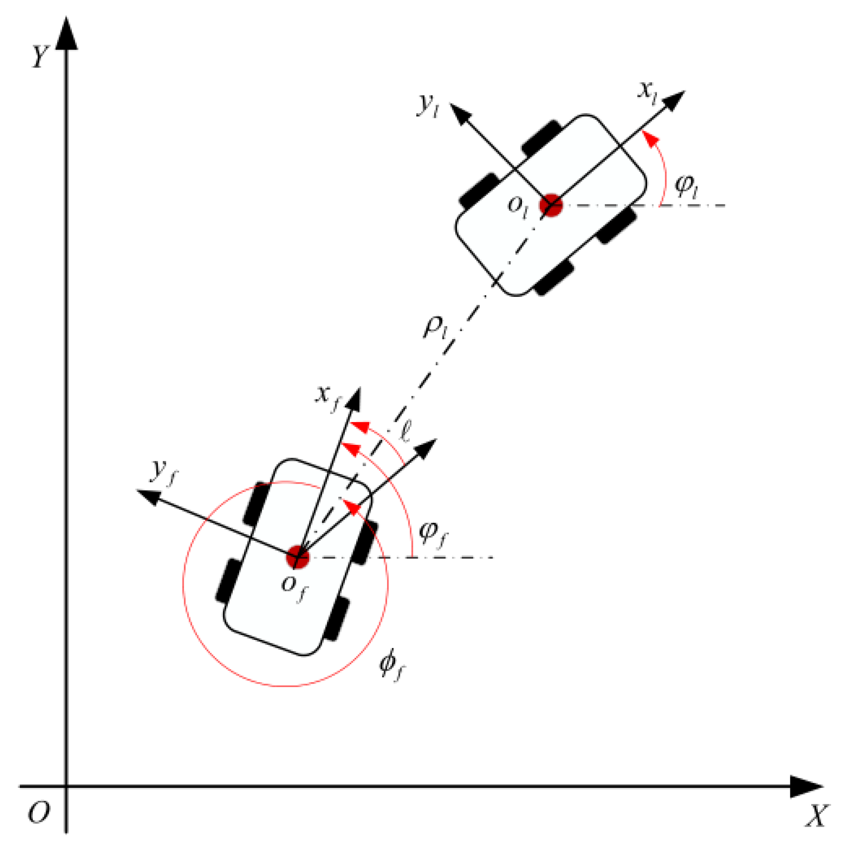
To facilitate problem analysis and control schemes design, this section first establishes a leader–follower formation model, as shown in Figure 1.

In Figure 1, $XOY$ denotes the global coordinate system; $x_i{o}_i{y}_i\left\{i=l,f\right\}$ denotes the body coordinate system, with the center of mass of the AGV as its origin. Where l denotes the subscript of the leader AGV, and f denotes the subscript of the follower AGV; ${\varphi }_f$ denotes the angle between the longitudinal axis of the follower AGV and the line connecting the centers of mass of the two AGVs; ${\phi }_l$ and ${\phi }_f$ denote the heading angles of the leader AGV and the follower AGV, respectively; ${\rho }_l$ denotes the distance from the center of mass of the follower AGV to that of the leader AGV; ℓ denotes the difference in heading angles between the leader AGV and the follower AGV. Based on the geometric relationships among the AGVs illustrated in Figure 1, the following expressions can be derived:

$$\left\{\begin{array}{c}{X}_l=X_f-{\rho }_l\cos \left({\phi }_f+{\varphi }_f\right)\hfill \\ Y_l=Y_f+{\rho }_l\sin \left({\phi }_f+{\varphi }_f\right)\hfill \\ {\phi }_l={\phi }_f+\mathcal{l}\hfill \end{array}\right.$$

(1)

When executing the formation task, the real-time desired coordinates of the leader and follower AGVs can be obtained via (1). The formation objective of this paper is to enable the dual AGVs to maintain a prescribed formation and follow the desired path cooperatively under port operation conditions. To this end, the formation control system must satisfy the following objective equations:

$$\left\{\begin{array}{c}{\lim }_{t\to T}{\mathit{P}}_l\left(t\right)={\lim }_{t\to T}{\mathit{P}}_l^d\left(t\right)\hfill \\ {\lim }_{t\to T}{\mathit{P}}_f\left(t\right)={\lim }_{t\to T}{\mathit{P}}_f^d\left(t\right)\hfill \end{array}\right.$$

(2)

The physical meaning of (2) is that the pose error between the leader and follower AGVs satisfies the formation system’s performance index within a finite time [43]. Specifically, as time evolves, the formation error converges asymptotically to the predefined bounded range. Here, $P_l={[X_l,Y_l,{\phi }_l]}^{\mathrm{T}}$ and $P_f={[X_f,Y_f,{\phi }_f]}^{\mathrm{T}}$ denote the actual poses of the leader and follower AGVs, respectively; $P_l^d={[X_l^d,Y_l^d,{\phi }_l^d]}^{\mathrm{T}}$ and $P_f^d={[X_f^d,Y_f^d,{\phi }_f^d]}^{\mathrm{T}}$ denote their desired poses, respectively.

2.2. Lateral Dynamics Modeling

In this study, a three-degree-of-freedom (3-DOF) planar dynamic model is adopted, considering the operational characteristics of port AGVs. These characteristics include flat and high-hardness road surfaces, frequent low-speed and heavy-load operations, high suspension stiffness, and minimal roll and center-of-mass variations during motion. To ensure the generality of the developed model, the following reasonable assumptions are made:

(1) All tires of the AGV are assumed to have identical characteristics and generate no aligning torque.

(2) The wheels on either side of the same AGV axle are assumed to exhibit identical motion states.

(3) The vertical, roll, and pitch motions of the AGV are neglected.

(4) The effects of lateral and longitudinal aerodynamics on the AGV’s yaw and longitudinal dynamics are neglected.

(5) Both the front and rear wheels of the AGV are assumed to be capable of independent steering.

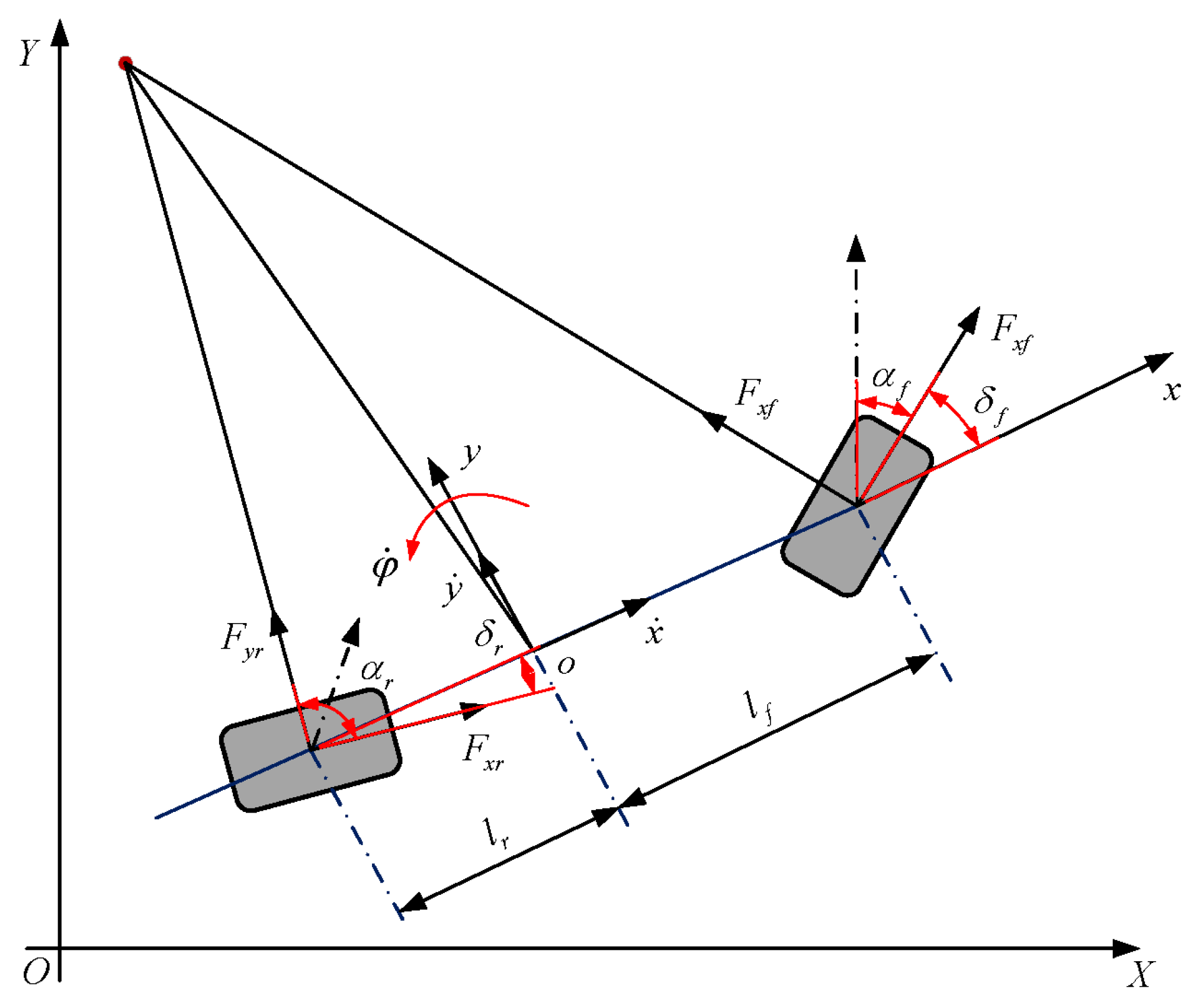
Based on the aforementioned assumptions, a lateral dynamics model for the dual-axle steering AGV is established, as illustrated in Figure 2.

In Figure 2, $XOY$ denotes the global coordinate system, and $xoy$ denotes the body-fixed coordinate system. The longitudinal forces acting on the front and rear tires are denoted by $F_{xf}$ and $F_{xr}$, respectively; the lateral forces by $F_{yf}$ and $F_{yr}$; the steering angles by ${\delta }_f$ and ${\delta }_r$; and the tire slip angles by ${\alpha }_f$ and ${\alpha }_r$. In addition, $\dot{x}$, $\dot{y}$, and $\dot{\phi }$ represent the longitudinal velocity, lateral velocity, and yaw rate, respectively, while $l_f$ and $l_r$ denote the distances from the front and rear axles to the center of mass.

By analyzing the force and moment equilibrium and accounting for external disturbances, the lateral dynamics model of the dual-axle steering AGV is derived as follows [18]:

$$\left\{\begin{array}{cc}\hfill \ddot{y}& =-{\displaystyle \frac{1}{m}}\left[F_{yf}\cos {\delta }_f+F_{yr}\cos {\delta }_r\right]-\dot{x}\dot{\phi }+d_y,\hfill \\ \hfill \ddot{\phi }& ={\displaystyle \frac{l_f}{I_z}}{F}_{yf}\cos {\delta }_f+{\displaystyle \frac{l_r}{I_z}}{F}_{yr}\cos {\delta }_r+d_{\phi }.\hfill \end{array}\right.$$

(3)

In (3), $d_y$ and $d_{\phi }$ represent the lateral and yaw disturbance inputs, respectively.

2.3. Longitudinal Dynamics Modeling

The longitudinal acceleration dynamics of the AGV can be modeled as a first-order inertial system, expressed as follows [44]:

$$\stackrel{⃛}{x}={\displaystyle \frac{1}{{\tau }_d}}({\ddot{x}}_{des}-\ddot{x})+d_x$$

(4)

In (4), $\ddot{x}$ represents the longitudinal acceleration, $\stackrel{⃛}{x}$ denotes its rate of change, ${\tau }_d$ is the time constant, and ${\ddot{x}}_{des}$ indicates the longitudinal acceleration control command. Additionally, $d_x$ accounts for the longitudinal disturbance. Based on Newton’s second law, the longitudinal dynamics of the AGV can be further described as follows:

$$\left\{\begin{array}{c}m\ddot{x}=F_{xf}+F_{xr}-F_{aero}-R_{xf}-R_{xr}-mgsin\vartheta \\ \stackrel{⃛}{x}={\displaystyle \frac{1}{{\tau }_d}}({\ddot{x}}_{des}-\ddot{x})+d_x\end{array}\right.$$

(5)

In (5), $F_{aero}$ denotes the equivalent aerodynamic resistance, $mgsin\vartheta$ represents the grade resistance, and $\vartheta$ is the road gradient. Considering that port AGVs operate on flat surfaces and do not travel at high speeds, the effects of both aerodynamic and grade resistance on longitudinal motion can be neglected. Consequently, (5) can be simplified as follows:

$$\left\{\begin{array}{c}m\ddot{x}=F_{xf}+F_{xr}-R_{xf}-R_{xr}\\ \stackrel{⃛}{x}={\displaystyle \frac{1}{{\tau }_d}}({\ddot{x}}_{des}-\ddot{x})+d_x\end{array}\right.$$

(6)

In (6), the rolling resistance forces $R_{xf}$ and $R_{xr}$ can be expressed as follows:

$$R_{xf}+R_{xr}=f_f(F_{zf}+F_{zr})$$

(7)

In (7), $f_f$ represents the rolling resistance coefficient, while $F_{zf}$ and $F_{zr}$ denote the vertical loads on the front and rear wheels, respectively.

3. Formation Control System Design

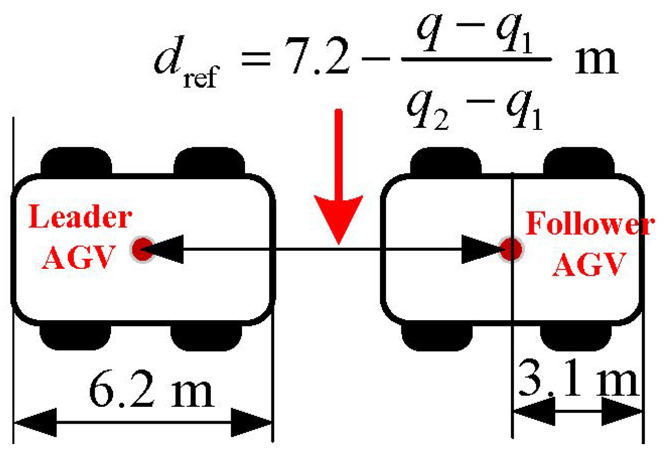
Port environments feature limited operating space. This study optimizes the formation model by dynamic adjustment of the vehicle spacing parameter to boost the maneuverability of an unloaded dual-AGV formation. The specific dynamic adjustment rules for formation spacing are as follows:

$$d_{\mathrm{ref}}=\left\{\begin{array}{c}7.2\mathrm{m},q\le q_1\\ 7.2-{\displaystyle \frac{q-q_1}{q_2-q_1}},q_1<q<q_2\\ 6.2,q\ge q_2\end{array}\right.$$

(8)

In (8), $d_{\mathrm{ref}}$ denotes the expected formation spacing, q represents road curvature, $q_1$ is the critical curvature for straight driving, and $q_2$ stands for the critical curvature for curve driving. This piecewise function improves the traditional fixed-spacing formation model by integrating real-time road curvature feedback. In contrast to conventional frameworks that rely on constant inter-vehicle distances, the proposed scheme dynamically adjusts the desired reference spacing according to the curvature parameter. Consequently, it eliminates the excessive turning radius caused by fixed long spacing during curve negotiation and significantly enhances the passing maneuverability of dual AGVs in narrow port lanes. The specific adjustment rules are classified into three operating conditions, as illustrated in Figure 3:

• When road curvature $q\le q_1=0.002{\mathrm{m}}^{-1}$ (straight road condition), the reference spacing is fixed at 7.2 m, which reserves sufficient safe distance for dual AGVs to transport standard 40-foot containers in straight sections;
• When the curvature satisfies $q_1<q<q_2=0.067{\mathrm{m}}^{-1}$, the reference spacing decreases linearly with the increase in curvature;
• When $q\ge q_2{\mathrm{m}}^{-1}$ (sharp curve), the minimum safe spacing 6.2 m is adopted to shrink the horizontal occupied width of the formation.

After this curvature-correlated spacing optimization, the overall turning radius of the dual-AGV formation is consistent with that of a single vehicle, effectively avoiding collision risks with yard-side barriers during curved driving.

This paper mainly investigates the control process of unloaded AGV formation traveling to the loading point. During this process, docking accuracy at loading points is the highest-priority subtask, as it directly affects operational efficiency. During loading operations, the influence of the formation’s lateral and longitudinal position errors on the spreader-AGV alignment time is significantly less pronounced than that of formation shape errors. (Herein, the formation error refers to the lateral or longitudinal deviation of the dual-AGV system as a whole relative to the desired trajectory. The formation shape error denotes the lateral or longitudinal error between individual AGVs within the formation). Among formation shape errors, the heading angle error exerts the most dominant effect. Consequently, the lateral controller should prioritize heading accuracy, while the longitudinal controller should emphasize both the convergence rate of formation errors and system response speed to enhance formation maintenance precision and operational safety. Furthermore, given that composite disturbances in the port environment exceed the suppression capability of conventional robust controllers, an FT-NDO is designed to accurately estimate system disturbances. These estimated disturbances are then integrated into the controller design to enhance the system’s anti-disturbance performance.

Based on the aforementioned control requirements, this section proposes a lateral SMC algorithm based on angular parameters and an NTSMC longitudinal control algorithm based on velocity parameters. The above lateral and longitudinal controllers are designed and applied under the condition of decoupled lateral and longitudinal motions of AGV. Acceleration and deceleration control is implemented during straight travel, while only steering control is adopted in turning motion. The relevant decoupling motion analysis is elaborated in our previously published literature [45]. The designed disturbance observer compensates for disturbances in the lateral and longitudinal control subsystems, respectively.

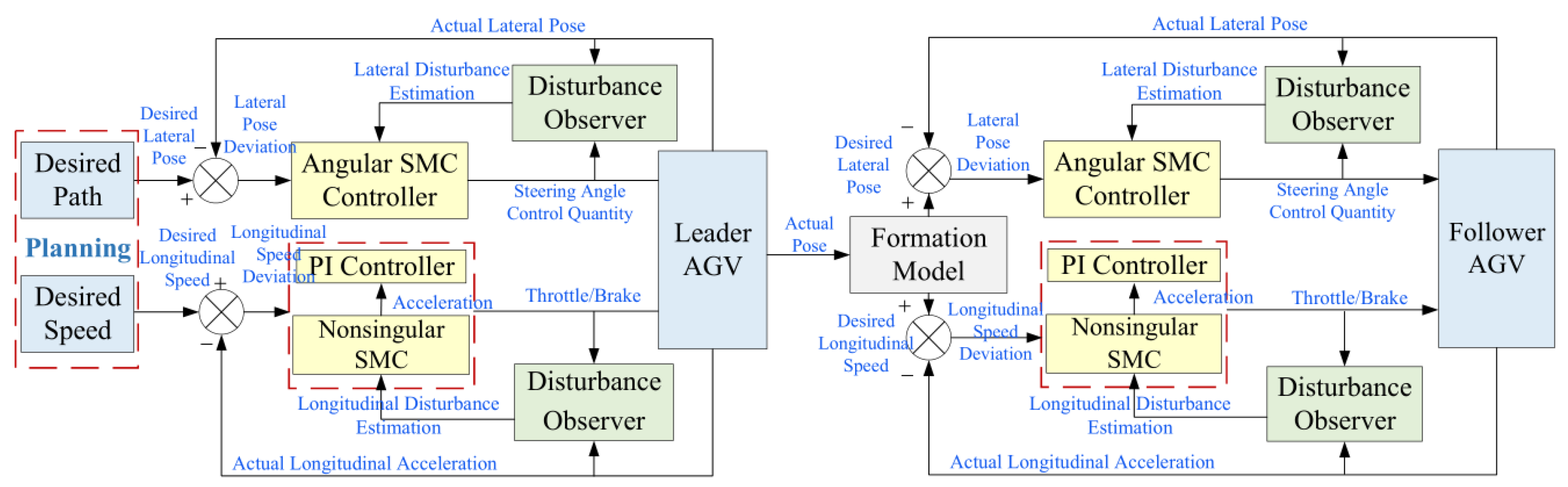
In summary, the overall structure of the formation control system is depicted in Figure 4. In accordance with the framework presented in the block diagram, the design process of the core controller will be elaborated in the subsequent subsections.

The complete robust formation control system constructed in this paper consists of five core functional modules: curvature-adaptive reference spacing generator, lateral SMC subsystem, longitudinal NTSMC subsystem, FT-NDO, and dual-AGV dynamic feedback module. The overall signal transmission logic of the framework is shown in Figure 4.

First, real-time road curvature q is collected to calculate the dynamic reference formation spacing $d_{\mathrm{ref}}$ via the piecewise adjustment rule in Equation (8), which outputs the expected relative pose between leader and follower AGVs. Second, the pose errors obtained by comparing the reference formation state and actual AGV feedback states are separately delivered to the lateral SMC and longitudinal NTSMC controllers. Third, the FT-NDO takes AGV motion states and preliminary control inputs as observation inputs, real-time estimates the composite lateral and longitudinal disturbances including pavement friction, inertial load, and unmodeled dynamics, and feeds the estimated disturbance values forward into both control loops for active compensation. Finally, the compensated steering angle and acceleration control commands are sent to the dual-AGV dynamic model, and the real-time motion states of the vehicles are fed back to the formation error calculation unit and disturbance observer to form a closed-loop control system. The lateral and longitudinal control channels are independently designed under the decoupling idea to avoid cross-coupling interference between horizontal steering and longitudinal velocity regulation.

3.1. A Finite-Time Nonlinear Disturbance Observer Design

In current engineering practice, two primary software-based approaches are widely employed to address disturbance-related issues:

(1)

Disturbance Rejection: This method relies on the inherent robustness and adaptability of control algorithms to passively counteract the effects of disturbance. Representative techniques include Proportional-Integral-Derivative (PID) control, SMC, and Model Predictive Control (MPC) [46,47]. However, such passive disturbance rejection strategies have inherent limitations: since control actions are only generated after disturbances occur, the resulting response lag often leads to significant system overshoot and compromised control accuracy in complex operational environments [48].

(2)

Disturbance Compensation: It achieves the suppression of system disturbances in the control feedforward loop by means of disturbance observation. Specific approaches include integrating various filters and disturbance observers into the control system. Such active anti-disturbance methods can enhance the real-time performance of the system and the error convergence rate, reduce system overshoot, and thereby render the control process more stable [49].

Accordingly, this subsection designs an FT-NDO to estimate disturbances in the AGV control system. The estimated disturbances are then integrated into the controller to achieve effective compensation and suppression of composite disturbances. Taking the lateral control subsystem as an example, the nominal lateral dynamics model established previously is reformulated into state-space form with explicit consideration of system disturbances:

$$\dot{\Gamma }=f(\Gamma )+g_1(\Gamma )u+g_2(\Gamma )d$$

(9)

In (9), $\Gamma ={[\dot{y},\dot{\phi }]}^{\mathrm{T}}$ denotes the state vector of the lateral control system, $f(\Gamma )$ and $g_1(\Gamma )$ represent the Jacobian matrices with respect to the state and input variables, respectively, and u is the control input vector. The term $d={[d_y,d_{\phi }]}^{\mathrm{T}}$ denotes the composite disturbances acting on the lateral control subsystem, where $d_y$ corresponds to the lateral motion disturbance and $d_{\phi }$ to the yaw motion disturbance of the AGV.

Let $\widehat{d}={[{\widehat{d}}_y,{\widehat{d}}_{\phi }]}^{\mathrm{T}}$ be the estimated value of the external disturbance, and define the disturbance estimation error as $\tilde{d}$, that is $\tilde{d}=d-\widehat{d}$. This instantaneous point-wise error $\tilde{d}$ is specially designed for Lyapunov-based finite-time stability proof of the observer. For global quantitative evaluation of overall observation accuracy, simulation analysis, additional statistical metrics including mean squared error (MSE) and mean absolute percentage error (MAPE) will be adopted to further quantify the estimation performance. Under normal operating conditions, the external disturbances affecting the AGV are bounded and vary slowly relative to the control process; it is therefore reasonable to assume that $\dot{d}\approx 0$. The finite-time disturbance observer is designed as [50]:

$$\dot{\widehat{d}}=-l(\Gamma )(\dot{\Gamma }-f(\Gamma )-g_1(\Gamma )u-g_2(\Gamma )\widehat{d})-\kappa {\left|\tilde{d}\right|}^{\alpha }\mathrm{sgn}(\tilde{d})$$

(10)

In (10), $l(\Gamma )\in {\mathbb{R}}^{2\times 2}$ is a positive definite gain matrix, $\kappa >0$ is the finite-time convergence gain, and $0<\alpha <1$ is the finite-time exponent. Substituting $\dot{d}\approx 0$ into the observer dynamics, the error system is derived as:

$$\dot{\tilde{d}}=-l(\Gamma )g_2(\Gamma )\tilde{d}-\kappa {\left|\tilde{d}\right|}^{\alpha }\mathrm{sgn}(\tilde{d})$$

(11)

To circumvent the difficulty in obtaining the differential signal of $\Gamma$ during the control process, an auxiliary function is introduced to reconstruct the disturbance observer. The auxiliary function is designed as follows:

$$\Delta =\dot{\Gamma }-f(\Gamma )-g_1(\Gamma )u$$

(12)

By combining (11) and (12), the differential form of $\widehat{d}$ can be expressed as:

$$\dot{\widehat{d}}=l(\Delta -g_2(\Gamma )\widehat{d})-\kappa {\left|\tilde{d}\right|}^{\alpha }\mathrm{sgn}(\tilde{d})$$

(13)

Stability Proof, choose the Lyapunov function candidate:

$$V={\displaystyle \frac{1}{2}}{\tilde{d}}^{\mathrm{T}}\tilde{d}$$

(14)

Taking the time derivative of V yields:

$$\dot{V}={\tilde{d}}^{\mathrm{T}}\dot{\tilde{d}}=-{\tilde{d}}^{\mathrm{T}}l(\Gamma )g_2(\Gamma )\tilde{d}-\kappa {\left|\tilde{d}\right|}^{\alpha +1}$$

(15)

Since $l(\Gamma )$ is positive definite, we have:

$$\dot{V}\le -{\lambda }_{1}V-{\lambda }_2{V}^{{\displaystyle \frac{\alpha +1}{2}}}$$

(16)

where ${\lambda }_1=2{\lambda }_{\min }\left(l(\Gamma )g_2(\Gamma )\right)>0$, ${\lambda }_2=\kappa {\left(\sqrt{2}\right)}^{\alpha +1}>0$, and $0<{\displaystyle \frac{\alpha +1}{2}}<1$. According to the finite-time stability theorem, the disturbance estimation error $\tilde{d}$ converges to zero in finite time:

$$T_f\le {\displaystyle \frac{2}{(1-\alpha ){\lambda }_2}}V{\left(0\right)}^{{\displaystyle \frac{1-\alpha }{2}}}$$

(17)

where $T_f$ is the upper bound of the convergence time. The proposed finite-time nonlinear disturbance observer is globally finite-time stable. It can accurately estimate and compensate for external disturbances within a finite time, which effectively enhances the anti-disturbance capability and dynamic performance of the dual-AGV formation system.

3.2. Design of Lateral SMC Controller Based on Angle Parameters

During the formation operation of dual AGVs, the heading angle control accuracy at loading points is assigned the highest priority. Accordingly, the lateral position error and heading angle error are selected as the core state variables for the lateral controller design, with particular emphasis on ensuring the convergence precision of the heading error. In the following, the leader AGV is taken as an example to illustrate the design procedure of the lateral controller. For notational simplicity, the subscript l denoting the leader AGV is omitted from all subsequent expressions.

The lateral position error $e_y$ and heading angle error $e_{\phi }$ of the leader AGV in the body-fixed coordinate system are defined as follows [51]:

$$\left\{\begin{array}{c}{y}_e=y_{ref}-y\\ {\phi }_e={\phi }_{ref}-\phi \end{array}\right.$$

(18)

To facilitate the design of the lateral SMC, a nonlinear switching function Z is formulated in terms of the lateral position error $y_e$ and the heading angle error ${\phi }_e$ as follows:

$$Z=c_0\tanh \left(c_1{y}_e\right)+{\phi }_e$$

(19)

In (19), parameters $c_0$ and $c_1$ are both positive real numbers, satisfying $0<c_0<\pi$ and $0<c_1<\pi$. Based on the above assumptions, it can be concluded that when Z approaches 0, $y_e$ and ${\phi }_e$ approaches 0 can be guaranteed. The specific proof process is as follows:

Define the Lyapunov function as $V={\displaystyle \frac{1}{2}}{y}_e^2$. Taking the derivative of this function yields: $\dot{V}=y_e\dot{y_e}=y_e\sqrt{{\dot{x}}^2+{\dot{y}}^2}sin(Z-c_{0}tanh\left(c_1{y}_e\right))$. When Z approaches 0, it can be further derived that: $\dot{V}=y_e\dot{y_e}=y_e\sqrt{{\dot{x}}^2+{\dot{y}}^2}sin(-c_{0}tanh\left(c_1{y}_e\right))$. Up to this point, the positivity or negativity of $\dot{V}$ can be discussed in three cases.

(1)

When $y_e<0$, it follows that $0<-c_{0}tanh\left(c_1{y}_e\right)<\pi$, $sin(-c_{0}tanh\left(c_1{y}_e\right))>0$, and thus $\dot{V}<0$.

(2)

When $y_e>0$, it follows that $-c_0<-c_{0}tanh\left(c_1{y}_e\right)<0$, $sin(-c_{0}tanh\left(c_1{y}_e\right))<0$, and thus $\dot{V}<0$.

(3)

When $y_e=0$, it can be obtained that $\dot{V}=0$.

In summary, $\dot{V}\le 0$ always holds for all feasible system states. That is, if the sliding function Z is driven to a value infinitely close to zero by the control law, the lateral position error $y_e$ and heading angle error ${\phi }_e$ will both decay and stay within a tiny neighborhood around zero. The negative semi-definite characteristic of $\dot{V}$ proves that the Lyapunov function $V={\displaystyle \frac{1}{2}}{y}_e^2$ is monotonically non-increasing throughout the system evolution. This guarantees that the magnitude of lateral error will not grow over time, and the heading error will be simultaneously restrained to a small range along with the vanishing sliding variable, which lays a solid theoretical foundation for the finite-time stability of the lateral control loop. Building upon the analytical result derived from (18), the switching function for the lateral SMC is designed as follows:

$$s=c_0\tanh \left(c_1{y}_e\right)+{\phi }_e$$

(20)

To mitigate system chattering and accelerate error convergence, the following exponential reaching law is adopted:

$$\dot{s}=-k_{s}s-k_{\epsilon }\mathrm{sgn}\left(s\right)$$

(21)

In (21), both $k_s$ and $k_{\epsilon }$ are positive real numbers. Differentiating (20) and combining it with (20) yields:

$$c_0{c}_1(1-{\tanh }^2\left(c_1{y}_e\right))\dot{y_e}+{\dot{\phi }}_e=-k_{s}s-k_{\epsilon }\mathrm{sgn}\left(s\right)$$

(22)

Combining (22) with (20) and substituting the disturbance estimation $\widehat{d}$ from the NDO for the actual disturbance in the lateral dynamics model, the control law $u={[{\delta }_f,{\delta }_r]}^{\mathrm{T}}$ can be derived. In accordance with the physical constraints of the AGV’s steering mechanism, a saturation function is applied to the wheel angle control command.

$$\left\{\begin{array}{cccc}\hfill {\delta }_i& =30°,\hfill & \hfill & \mathrm{if}{\delta }_i\ge 30°,\{i=f,r\},\hfill \\ \hfill {\delta }_i& ={\delta }_i,\hfill & \hfill & \mathrm{if}-30°\le {\delta }_i\le 30°,\{i=f,r\},\hfill \\ \hfill {\delta }_i& =-30°,\hfill & \hfill & \mathrm{if}{\delta }_i\le -30°,\{i=f,r\}.\hfill \end{array}\right.$$

(23)

Stability Analysis: We conduct Lyapunov stability analysis here to verify that the proposed exponential reaching law can drive the sliding variable to 0 within finite time, and further constrain the lateral position error and heading angle error within a small neighborhood after sliding motion is formed.

Define the Lyapunov function:

$$V={\displaystyle \frac{1}{2}}{s}^2$$

(24)

Clearly, $V\ge 0$ and $V=0$⟺$s=0$. Differentiating V yields:

$$\dot{V}=s(-k_{s}s-k_{\epsilon }\mathrm{sgn}\left(s\right))=-k_s{s}^2-k_{\epsilon }\left|s\right|$$

(25)

Using $s^2=2V$. $\left|s\right|=\sqrt{2V}$, rewrite as:

$$\dot{V}=-2k_{s}V-k_{\epsilon }\sqrt{2V}$$

(26)

Define ${\lambda }_1=2k_s>0$, ${\lambda }_2=k_{\epsilon }\sqrt{2}>0$, $\gamma ={\displaystyle \frac{1}{2}}\in (0,1)$. Then:

$$\dot{V}\le -{\lambda }_{1}V-{\lambda }_2{V}^{\gamma }$$

(27)

From (28), drop the negative definite term $-{\lambda }_{1}V$ to obtain:

$$\dot{V}\le -{\lambda }_2{V}^{\gamma }$$

(28)

Since $V>0$ before convergence, divide both sides by $V^{\gamma }>0$:

$$V^{-\gamma }\dot{V}\le -{\lambda }_2$$

(29)

Integrate both sides from $t=0$ to $t=T$:

$${\int }_{V\left(0\right)}^{V\left(T\right)}{V}^{-\gamma }dV\le -{\lambda }_{2}T$$

(30)

Compute the integral, ${\displaystyle \frac{V{\left(0\right)}^{1-\gamma }-V{\left(T\right)}^{1-\gamma }}{1-\gamma }}\le -{\lambda }_{2}T$. Set $V\left(T\right)=0$, $-{\displaystyle \frac{V{\left(0\right)}^{1-\gamma }}{1-\gamma }}\le -{\lambda }_{2}T$. Cancel the minus sign:

$$T\le {\displaystyle \frac{V{\left(0\right)}^{1-\gamma }}{{\lambda }_2(1-\gamma )}}$$

(31)

Substitute $\gamma =1/2$, ${\lambda }_2=k_{\epsilon }\sqrt{2}$:

$$T\le {\displaystyle \frac{\sqrt{2V\left(0\right)}}{k_{\epsilon }}}$$

(32)

After the above derivation, it can be confirmed that the sliding variable s converges to 0 in finite time T. When $s=0$ holds, $c_0\tanh \left(c_1{y}_e\right)+{\phi }_e=0$ is satisfied, which means both lateral error $y_e$ and heading angle error ${\phi }_e$ will decay to the vicinity of 0. Thus, the lateral control system achieves global finite-time stability.

3.3. Design of Longitudinal Controller Based on Nonsingular Terminal SMC

Regarding the longitudinal controller design for the unloaded dual-AGV formation system, two critical challenges must be urgently addressed. (1) Due to the standardized dimensions of containers, when the dual AGVs move toward the loading point in an unloaded formation to transport a 40-foot container, the distance between the tail of the leader AGV and the head of the follower AGV is only 1 m. This necessitates a longitudinal control system with fast response capability to prevent collisions caused by excessive speed errors between the AGVs in the formation. (2) External disturbances in the port environment significantly affect the longitudinal speed control accuracy of the AGVs. To improve formation synchronization and ensure operational safety, the longitudinal control system must exhibit strong robustness. To address these challenges, this subsection proposes a longitudinal controller based on NTSMC, which computes control commands by incorporating disturbance estimates provided by the longitudinal disturbance observer.

Based on the AGV longitudinal dynamics model established in Section 2, this subsection formulates a second-order dynamic model with explicit consideration of longitudinal disturbances. This formulation facilitates both disturbance estimation via the previously designed observer and the development of the NTSMC scheme. The resulting second-order longitudinal dynamics model subject to disturbances is given as follows [52]:

$$\left\{\begin{array}{c}\hfill {\dot{x}}_{s1}=\dot{x}\\ \hfill {\dot{x}}_{s2}=f_d+u=\ddot{x}\\ \hfill y_o=x\end{array}\right.$$

(33)

In (33), x represents the longitudinal displacement of the AGV, and $\dot{x}$ denotes its longitudinal velocity. The term $f_d$ indicates the composite disturbance in the longitudinal system, while u is the control input, defined as $u={\ddot{x}}_{des}$. The state variables of the longitudinal control system are denoted by $x_{s1}$ and $x_{s2}$, and $y_0$ represents the system output.

The design and stability analysis of the FT-NDO have been thoroughly presented in Section 3.1. The same observer structure can be directly applied to estimate the longitudinal disturbance $f_d$ of the AGV, and thus its detailed implementation is omitted here for brevity. The subsequent discussion focuses on the design procedure and stability proof of the NTSMC strategy. Specifically, the nonsingular terminal sliding surface is designed as follows [53]:

$$s=x_{s1}+k_{\alpha }{x}_{s_2}^{k_{\beta }}$$

(34)

In (34), $k_{\alpha }$ and $k_{\beta }$ are both gain parameters, where $k_{\alpha }>0,1<k_{\beta }<2$. The control law of the NTSMC is composed of two components: an equivalent control term and a nonlinear switching term. The equivalent control term is derived from the sliding surface dynamics, ensuring that the system states can slide along the surface under nominal conditions and maintain sliding motion even in the presence of disturbances. In contrast, the nonlinear switching term is designed to provide additional control effort for counteracting disturbances and uncertainties in the longitudinal system. This ensures that the system states can rapidly reach and maintain sliding motion on the prescribed surface, even in the presence of such adverse effects [54]. This approach significantly enhances the robustness of the longitudinal control system and mitigates deviations induced by disturbances and uncertainties. Accordingly, the overall control law is formulated as follows:

$$u=u_{eq}+u_n$$

(35)

In (35), $u_{eq}$ denotes the equivalent control term, and $u_n$ denotes the nonlinear control term. The derivative of (34) yields $\dot{s}$ as follows:

$$\dot{s}={\dot{x}}_{s1}+k_{\alpha }{k}_{\beta }{x}_{s2}^{k_{\beta }-1}{\dot{x}}_{s2}$$

(36)

When $\dot{s}=0$ in (36), the equivalent control term of the NTSMC is derived as follows:

$$u_{eq}={\displaystyle \frac{-x_{s2}}{k_{\alpha }{k}_{\beta }{x}_{s2}^{k_{\beta }-1}}}-{\widehat{f}}_d$$

(37)

In (37), ${\widehat{f}}_d$ represents the estimated longitudinal disturbance obtained from the FT-NDO. To further improve the convergence rate of the control system, an exponential reaching law in the form of (36) is designed and combined with (35), yielding the following nonlinear switching term:

$$u_n={\displaystyle \frac{-k_{s}s-k_{\epsilon }\mathrm{sgn}\left(s\right)-x_{s2}}{k_{\alpha }{k}_{\beta }{x}_{s2}^{k_{\beta }-1}}}-{\widehat{f}}_d$$

(38)

By combining (37) and (38), the control law of the NTSMC is obtained as follows:

$$u={\displaystyle \frac{-k_{s}s-k_{\epsilon }\mathrm{sgn}\left(s\right)-2x_{s2}}{k_{\alpha }{k}_{\beta }{x}_{s2}^{k_{\beta }-1}}}-2{\widehat{f}}_d$$

(39)

In accordance with the operational characteristics of port AGVs, the following saturation function is applied to their longitudinal acceleration control commands:

$$\left\{\begin{array}{cccc}\hfill {\ddot{x}}_{\mathrm{des}}& =+1.0\mathrm{m}/{\mathrm{s}}^2,\hfill & \hfill & \mathrm{if}{\ddot{x}}_{\mathrm{des}}\ge +1.0\mathrm{m}/{\mathrm{s}}^2,\hfill \\ \hfill {\ddot{x}}_{\mathrm{des}}& ={\ddot{x}}_{\mathrm{des}},\hfill & \hfill & \mathrm{if}-1.0\mathrm{m}/{\mathrm{s}}^2<{\ddot{x}}_{\mathrm{des}}<+1.0\mathrm{m}/{\mathrm{s}}^2,\hfill \\ \hfill {\ddot{x}}_{\mathrm{des}}& =-1.0\mathrm{m}/{\mathrm{s}}^2,\hfill & \hfill & \mathrm{if}{\ddot{x}}_{\mathrm{des}}\le -1.0\mathrm{m}/{\mathrm{s}}^2.\hfill \end{array}\right.$$

(40)

To analyze the stability of the proposed controller, consider the Lyapunov function candidate $V={\displaystyle \frac{1}{2}}{s}^2$. Its time derivative is given by:

$$\dot{V}=s(-k_{s}s-k_{\epsilon }\mathrm{sgn}\left(s\right))=-k_s{s}^2-k_{\epsilon }\left|\begin{array}{c}s\end{array}\right|$$

(41)

We rewrite $\dot{V}$ as $\dot{V}=-2k_{s}V-k_{\epsilon }\sqrt{2V}$. Define ${\lambda }_1=2k_s>0$, ${\lambda }_2=k_{\epsilon }\sqrt{2}>0$, and $\gamma =1/2\in (0,1)$. Then, $\dot{V}\le -{\lambda }_2{V}^{\gamma }$. Dropping the negative definite term $-{\lambda }_{1}V$, we have $\dot{V}\le -{\lambda }_2{V}^{\gamma }$. Since $V>0$ before convergence, dividing both sides by $V^{\gamma }>0$ yields $V^{-\gamma }\dot{V}\le -{\lambda }_2$. Integrating both sides from $t=0$ to $t=T$, we obtain ${\int }_{V\left(0\right)}^{V\left(T\right)}{V}^{-\gamma }dV\le -{\lambda }_{2}T$. Evaluating the integral and setting $V\left(T\right)=0$, it follows that $T\le {\displaystyle \frac{V{\left(0\right)}^{1-\gamma }}{{\lambda }_2(1-\gamma )}}={\displaystyle \frac{\sqrt{2V\left(0\right)}}{k_{\epsilon }}}$. Thus, s converges to 0 in finite time.

4. Simulation and Analysis of No-Load Formation

The theoretical deterministic stability analysis in Section 3 only verifies the finite-time convergence property of the proposed controller under ideal mathematical simplifications, but cannot quantify transient tracking errors, steering oscillation, and disturbance suppression performance under real nonlinear AGV dynamics. Therefore, a Matlab/Simulink-TruckSim co-simulation platform is constructed to reproduce port time-varying curved roads and low-frequency composite disturbances. This platform enables repeatable quantitative performance comparison among different control schemes, serving as a critical intermediate verification step between theoretical deduction and physical prototype experiments. The simulation study is organized into the following two parts to comprehensively evaluate the performance of the proposed approach:

(1)

Robustness Verification: This simulation aims to evaluate the effectiveness of the designed disturbance observer. To emulate the complex interference environment in ports, external disturbance signals are injected into the formation control system. The control performance of the dual-AGV formation is compared under two operating scenarios: with and without the disturbance observer. Through comparative analysis, the specific contribution of the observer to enhancing the disturbance rejection capability of the formation system is quantitatively assessed.

(2)

Control Scheme Comparison: This set of simulations conducts a comprehensive comparison between the proposed formation control scheme and existing mainstream robust formation control methods. The evaluation aims to demonstrate the advantages of the proposed approach in terms of robustness, control accuracy, and error convergence speed.

4.1. Robustness Test of the Control System

Prior to the simulation, the inter-vehicle distance between the rear axle centers of the leader and follower AGVs is configured as 7.2 m. After accounting for the front and rear overhangs of individual vehicles, this corresponds to a 1 m distance between the tail of the leader AGV and the head of the follower AGV. The leader AGV is initially positioned at (0, 0, 0), while the follower AGV is located at (0, −7.2, 0) in the global coordinate system. Upon simulation start, the AGV formation begins from a stationary state, accelerates at 1 $\mathrm{m}/{\mathrm{s}}^2$ for 6 s, maintains a constant speed for 5 s, then decelerates at −1 $\mathrm{m}/{\mathrm{s}}^2$ for 2 s, followed by constant-speed travel through a 15 m radius curve. Subsequently, the formation accelerates again at 1 $\mathrm{m}/{\mathrm{s}}^2$ for 2 s, continues at constant speed for 5 s, decelerates at −1 $\mathrm{m}/{\mathrm{s}}^2$ for 2 s, and then maintains constant speed for 9 s while negotiating a second curve with a radius of 15 m. Finally, the formation decelerates to a complete stop at −1 $\mathrm{m}/{\mathrm{s}}^2$. The entire simulation lasts 40 s, with a road adhesion coefficient of 0.85. The key performance parameters of the AGV are listed in

Table 2. Main parameter configuration of formation AGVs.

Parameter Name	Value	Unit
Mass	15	t
Wheelbase	5.0	m
Distance from center of mass to front/rear axle	2.5/2.5	m
Moment of inertia about z-axis	117,180.4	kg·m2
Longitudinal stiffness of front/rear wheels	150,000/150,000	N/rad
Cornering stiffness of front/rear wheels	259,752/259,752	N/rad
Slip ratio of front/rear wheels	0.2/0.2	-
Maximum steering angle of front/rear wheels	0.52	rad
Maximum steering angle rate of front/rear wheels	0.17	rad/s

.

Considering that the heading angle of the port AGV formation remains within the range of $[0,\pi ]$ and the longitudinal speed varies between 0 and 6 $\mathrm{m}/\mathrm{s}$ during operation, the lateral and longitudinal disturbances acting on the formation system are specified as $d_1=1.5\sin \left(5t\right)$ and $d_2=3\cos \left(2t\right)$ [55,56], which are low-frequency sinusoidal/cosine signals with angular frequencies of 5 rad/s and 2 rad/s, respectively. These frequencies are significantly lower than the control bandwidth of the proposed scheme. Consequently, the time derivatives of the disturbances $d_1$ and $d_2$ remain small throughout the simulation, satisfying the slow-varying assumption $\dot{d}\approx 0$ adopted in the finite-time nonlinear disturbance observer design. Such low-frequency disturbances reasonably reflect real-world port uncertainties, including wind gusts, uneven ground friction, and load variations. The core parameters of each controller are configured as follows: the gain matrix of the FT-NDO is set as $l(\Gamma )={[15,5;2,6]}^{\mathrm{T}}$, $\kappa =1.25$, $\alpha =0.36$; the key parameters of the lateral SMC are $c_0=2.8$, $c_1=0.12$, $k_s=132$, and $k_{\epsilon }=1.75$; the essential parameters of the longitudinal NTSMC are $k_{\alpha }=0.03$, $k_{\beta }=1.15$. The core gains of the lateral/longitudinal sliding mode controller and FT-NDO are finalized after abundant iterative simulation trials, and their impacts on tracking performance, system stability, and anti-disturbance capacity follow clear rules:

• Increasing the reaching law gain accelerates the convergence speed of tracking errors and strengthens disturbance suppression ability, yet excessively large values will introduce severe control chattering and threaten system stability;
• Larger sliding surface weighting coefficients can prioritize heading angle tracking precision during AGV turning, but may slightly sacrifice lateral position response speed;
• Higher gains of the finite-time disturbance observer can realize faster disturbance estimation, while overly high observer gains amplify measurement noise and lead to oscillatory estimation residuals.

The group of gains adopted in this paper strikes a balanced trade-off among fast error convergence, mild control chattering, and reliable noise immunity after repeated testing under curved trajectory and time-varying disturbance conditions. The corresponding simulation results are presented in Figure 5, Figure 6, Figure 7, Figure 8, Figure 9, Figure 10, Figure 11 and Figure 12.

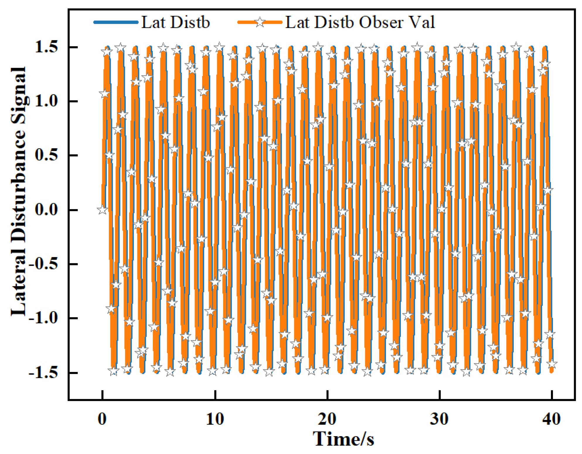
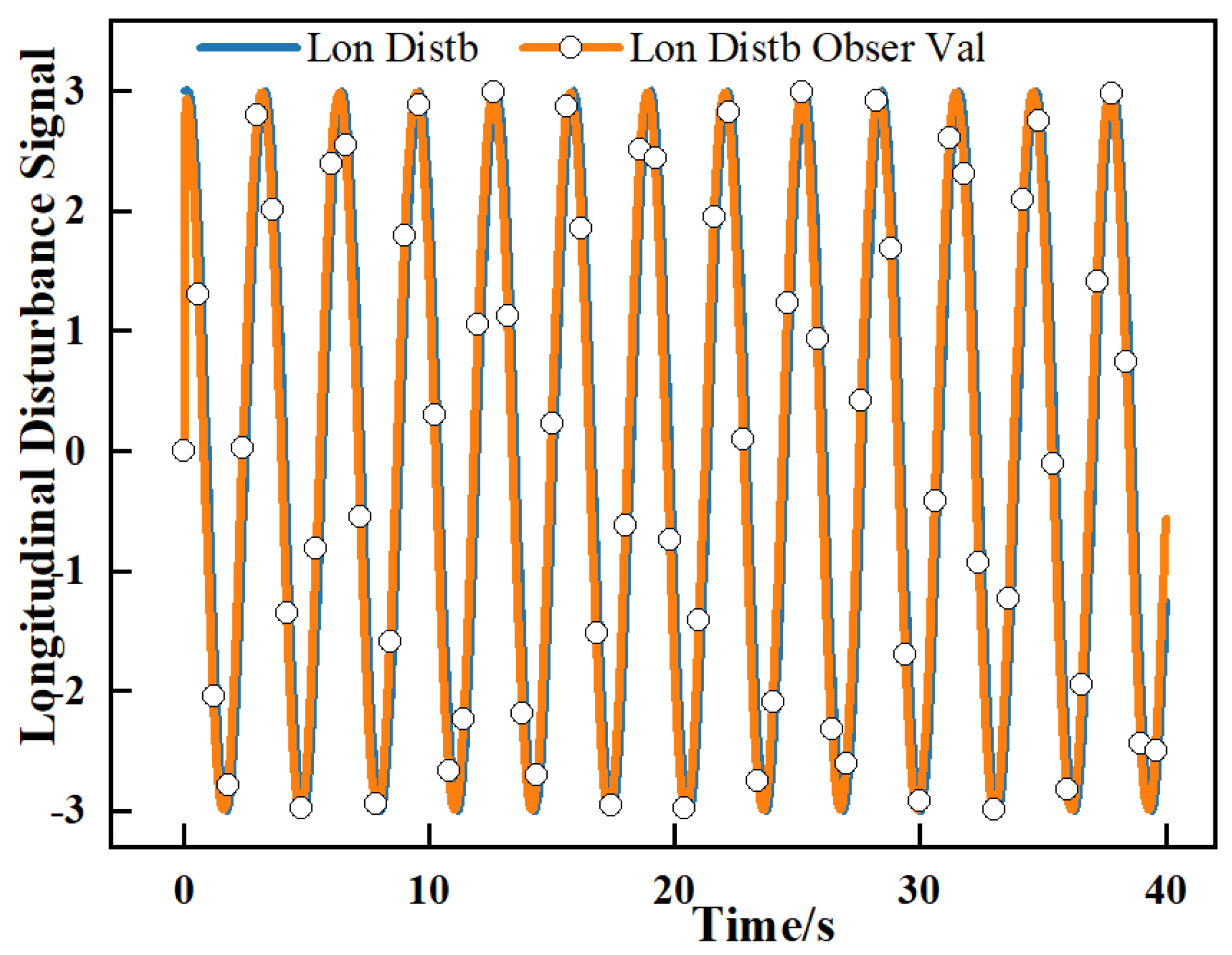
Figure 5 and Figure 6 present the simulated external disturbance signals and their corresponding estimates obtained by the FT-NDO, respectively. Since both AGVs in the formation employ identical disturbance observers, the leader AGV’s reference and observed data are used as representative examples for analysis. For improved clarity in the figure, abbreviated labels are adopted in Figure 5 and Figure 6. In the figures, “Lat Distb” denotes the lateral disturbance, while “Lat Distb Obser Val” indicates the lateral disturbance observation value. Similarly, “Lon Distb” refers to the longitudinal disturbance, and “Lon Distb Obser Val” represents the longitudinal disturbance observation value. The same naming convention applies to subsequent figures and will not be reiterated hereafter. The data presented in Figure 5 demonstrate that throughout the entire simulation process, the FT-NDO designed in this study achieves accurate estimation of the actual external disturbances, with the observed disturbance curves closely tracking the reference profiles. As shown in Figure 6, during the initial phase $0\le t\le 1.5$ s, the disturbance observer exhibits relatively large estimation errors. However, these errors converge rapidly after $t=1.5$ s, resulting in close agreement between the observed and reference disturbance values thereafter.

The observed discrepancies in estimation accuracy between lateral and longitudinal disturbances stem primarily from the following aspects: (1) The lateral dynamics of AGVs are predominantly governed by steering control, where the coupling between steering-related variables (e.g., yaw rate) and external disturbances is more direct and readily discernible in the dynamic model. As a result, disturbance information during the initial phase is more readily captured, facilitating rapid observer calibration and consequent reduction of initial estimation errors. (2) In contrast, longitudinal control prioritizes velocity tracking stability, typically implemented with conservative parameter settings. This leads to a slower system response, making it difficult for the disturbance observer to promptly adjust its estimates based on control deviations during the initial transient period.

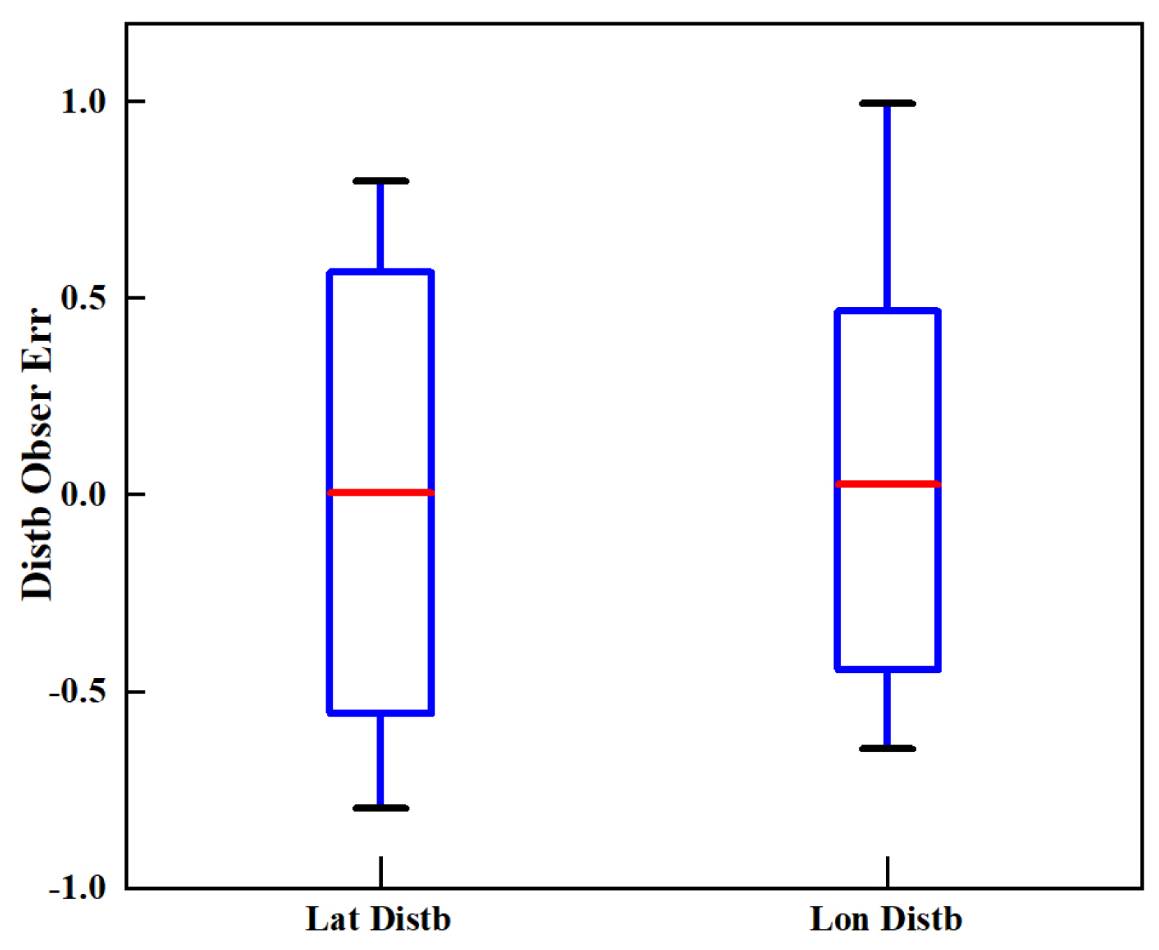
Figure 7 displays the distributions of lateral and longitudinal disturbance observation errors. Both lateral and longitudinal errors exhibit medians sufficiently close to zero with narrow interquartile ranges, and the majority of errors are concentrated within the [−0.5, 0.5] interval. To further quantitatively assess the overall disturbance observation accuracy beyond instantaneous deviation $\tilde{d}$, we calculate the MSE and MAPE of lateral and longitudinal disturbance estimation over the full 40 s simulation period:

• Lateral disturbance estimation: MSE = 0.042, MAPE = 3.86%;
• Longitudinal disturbance estimation: MSE = 0.051, MAPE = 4.23%.

The low MSE and MAPE values consistently demonstrate that the proposed FT-NDO achieves estimation accuracy exceeding 95% for both lateral and longitudinal composite disturbances, which is consistent with the narrow error distribution shown in Figure 7. MSE reflects the overall fluctuation magnitude of estimation residuals, while MAPE eliminates the influence of disturbance amplitude to provide a normalized accuracy reference, jointly supporting the reliability of the designed disturbance observer. These results demonstrate that the FT-NDO achieves high-precision disturbance estimation, which is crucial for maintaining the excellent lateral stability and velocity tracking capability of the AGV formation in complex port environments. This high estimation accuracy significantly reduces overshoot and tracking errors induced by external composite disturbances in the formation system.

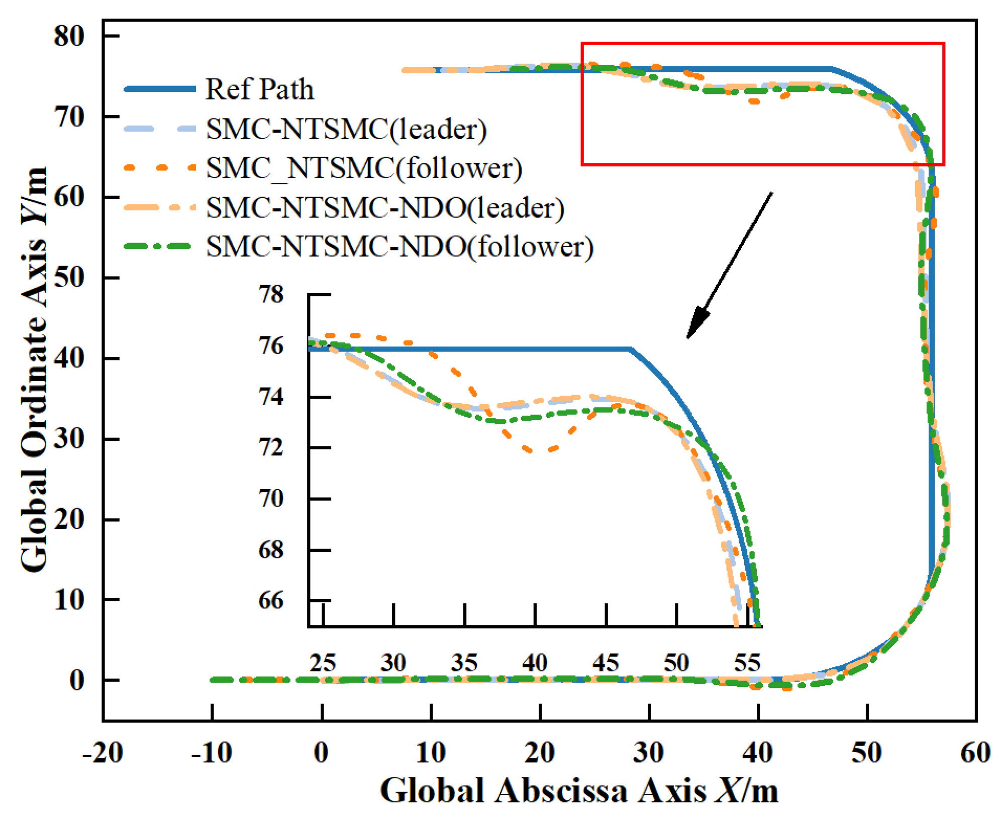
Figure 8 compares the formation operation performance with and without the disturbance observer. For clarity: “Ref Path” indicates the reference path; “SMC-NTSMC (leader)” and “SMC-NTSMC (follower)” denote the trajectories of the leader and follower AGVs, respectively, using only the SMC. Meanwhile, “SMC-NTSMC-NDO (leader)” and “SMC-NTSMC-NDO (follower)” represent the corresponding trajectories when the FT-NDO is integrated with the controllers.

As shown in Figure 8, when the AGV formation operates under external disturbances, the proposed SMC-NTSMC-NDO scheme demonstrates strong robustness. On the straight road segment (0–40 m), both control schemes maintain high straight-line tracking accuracy, indicating that the baseline SMC-NTSMC controllers already possess considerable robustness. However, a notable performance divergence emerges when the formation enters curved sections. Taking the second curve as an example, the formation under the baseline SMC-NTSMC scheme exhibits significant oscillatory behavior, with the follower AGV displaying a sinusoidal swinging motion. In contrast, the SMC-NTSMC-NDO scheme maintains high formation accuracy throughout the curve negotiation.

Owing to the optimized leader–follower formation model proposed in this study—which dynamically adjusts the desired inter-vehicle spacing according to road curvature—the AGVs exhibit highly overlapping trajectories. An in-depth analysis reveals that the oscillatory behavior observed under the SMC-NTSMC scheme in curved sections stems from two main factors: First, the disturbance rejection capability of the baseline lateral and longitudinal SMC controllers is limited. The cumulative errors induced by external disturbances progressively degrade the performance of the motion controllers. Second, the follower AGV is subjected to more severe disturbances than the leader. In addition to external disturbances, the follower also experiences disturbances caused by formation model inaccuracies. The superposition of these disturbances exceeds the robustness margin of the baseline SMC controller. These findings highlight the practical importance of enhancing the robustness of the formation control system, particularly its string stability. Improved robustness is not only essential for ensuring operational stability and scalability, but also a critical prerequisite for maintaining safe formation control in real-world applications.

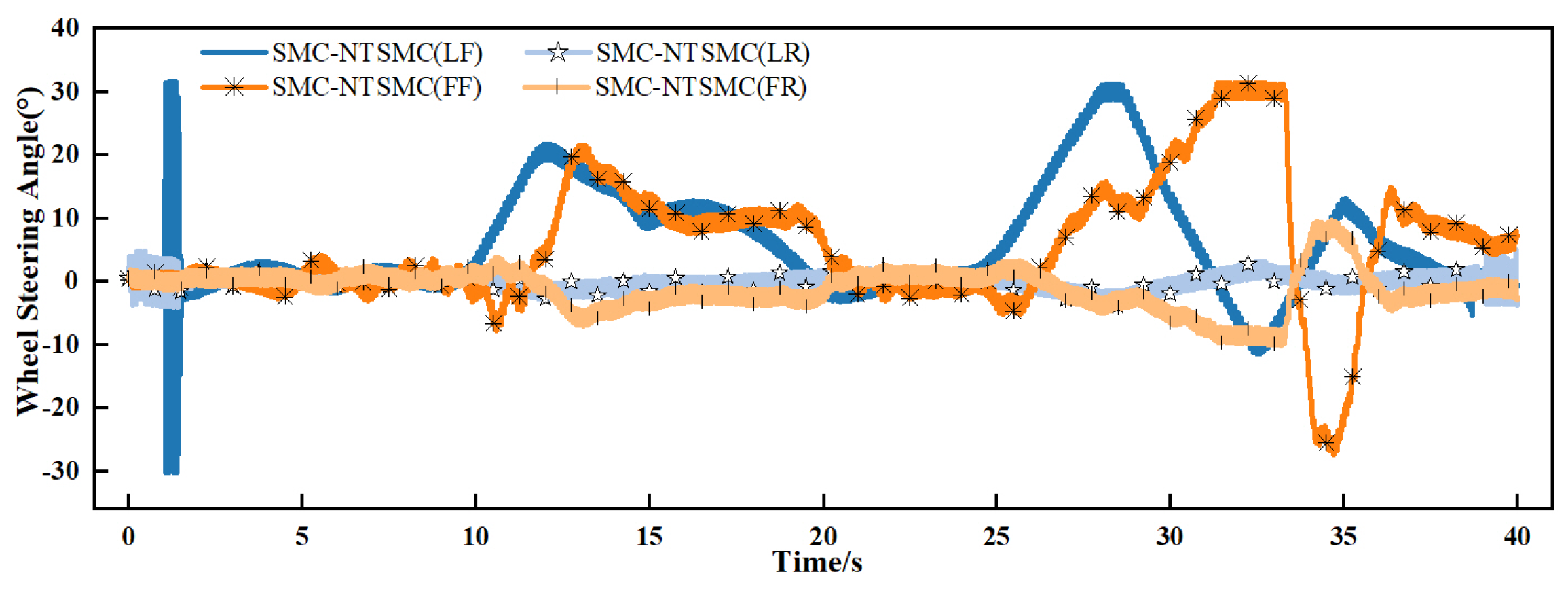
Figure 9 illustrates the steering angle variations of the wheels for both AGVs in the formation. In the figure, “LF” denotes the front wheel of the leader AGV, “LR” represents its rear wheel, “FF” indicates the front wheel of the follower AGV, and “FR” refers to the rear wheel of the follower AGV. The same naming convention applies to subsequent figures and will not be reiterated.

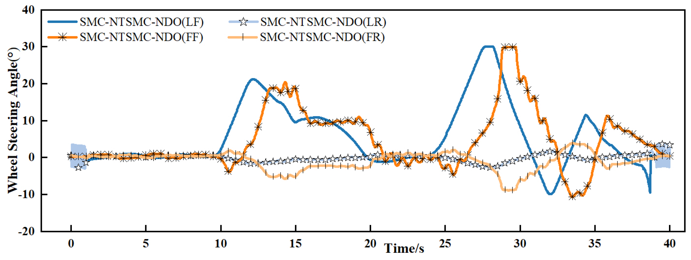
The data in Figure 9 reveal that under the SMC-NTSMC scheme, the formation AGVs experience high-frequency wheel oscillations with large amplitudes during both the initial acceleration and curve negotiation phases. For instance, the leader AGV’s front-wheel oscillation reaches 60° during initial acceleration, while the follower AGV’s front wheel exhibits 50° oscillations in the second curve. Such severe steering oscillations considerably compromise formation stability and subject tires and related components to substantial impact loads. In contrast, as demonstrated in Figure 10, the SMC-NTSMC-NDO scheme enables significantly smoother steering operation throughout most of the trajectory. Only minor steering jitters are observed during the initial and final simulation phases.

These comparative results demonstrate that the disturbance rejection capability of the standalone SMC controller is limited, rendering it inadequate for effectively handling complex disturbance environments. Relying solely on this controller for passive disturbance suppression tends to induce oscillatory behavior in the formation system. However, when integrated with an FT-NDO, the control system exhibits significantly enhanced robustness and disturbance rejection performance, substantially improving the operational stability of the AGV formation in practical port environments.

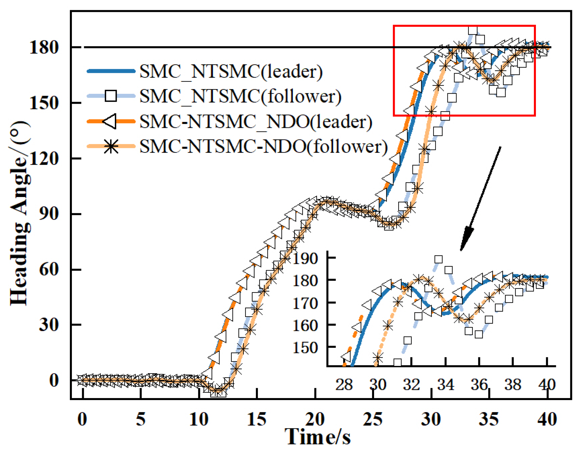
As evidenced by the data in Figure 11, the dual-AGV formation maintains high control accuracy under the SMC-NTSMC-NDO scheme. Specifically, the leader and follower AGVs exhibit highly consistent heading angle variations with minimal influence from external disturbances. Furthermore, the heading angle transitions remain smooth throughout the trajectory, aligning well with the stable steering behavior observed in Figure 9 and Figure 10. At the loading docking position, the formation achieves an attitude error of ±0.5°, satisfying the precision requirements for automated port operations.

In contrast, under the SMC-NTSMC scheme, the formation develops substantial attitude errors, particularly in the second curve section. This primarily results from the backward propagation of the leader AGV’s motion errors, which exceeds the compensation capability of the follower’s controller.

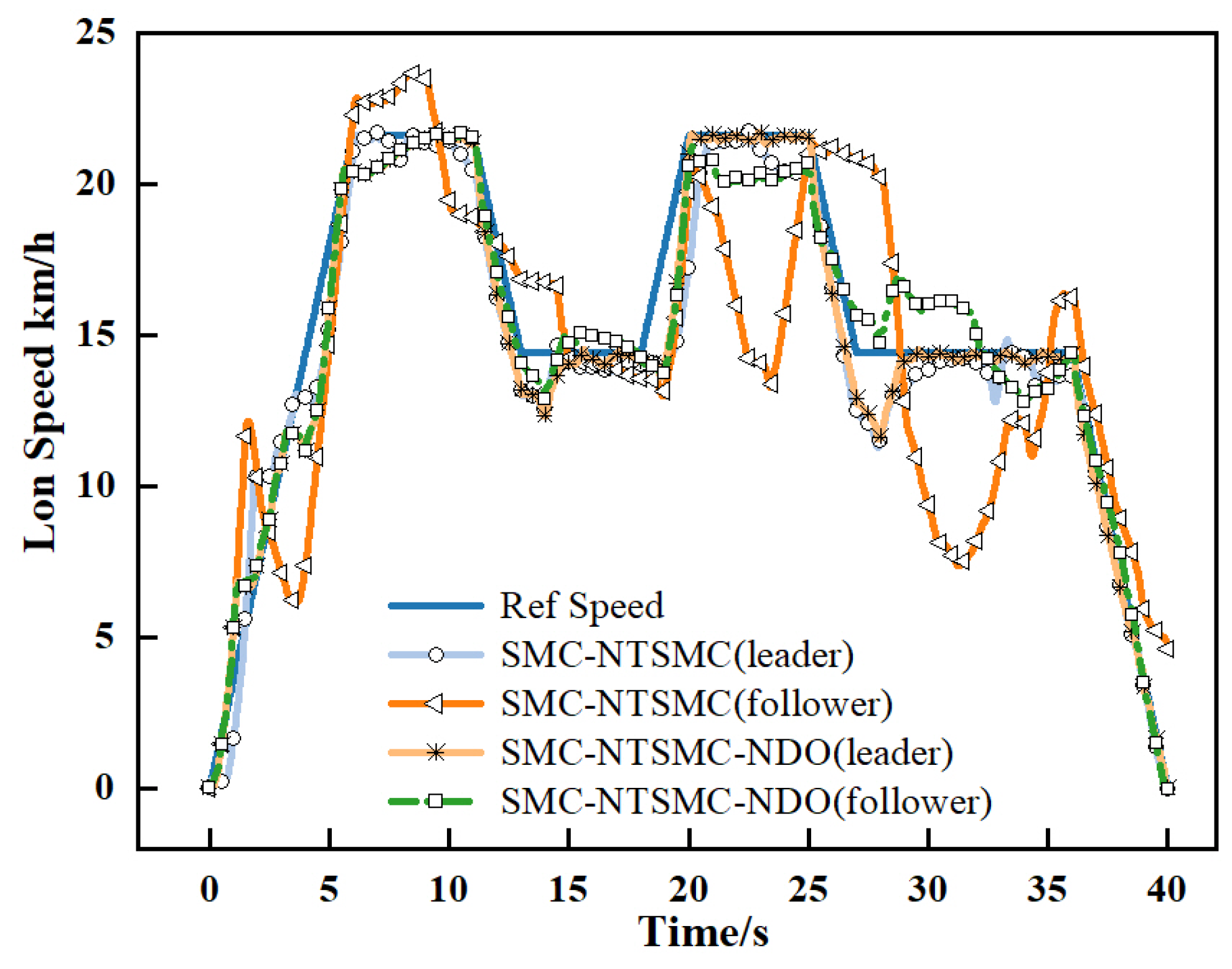
Figure 12 illustrates the longitudinal velocity profiles of the formation AGVs. The results demonstrate that the SMC-NTSMC-NDO scheme achieves satisfactory motion synchronization, with a steady-state velocity error of only 0.015 km/h between the AGVs, confirming its high formation-keeping precision. However, when negotiating the second curve, the follower AGV exhibits a velocity lag relative to the leader, followed by a speed overshoot upon returning to the straight section. Ultimately, both AGVs achieve smooth and synchronized stopping at the loading point.

Analysis of the observed velocity discrepancies reveals two primary causes. First, cumulative errors during acceleration, deceleration, and curve negotiation alter the inter-vehicle spacing. The high responsiveness of the NTSMC controller prompts rapid speed adjustments in the follower to correct these spacing deviations, resulting in temporary velocity inconsistencies. Second, suboptimal parameter tuning in the longitudinal controller may require further refinement to minimize such compensatory actions.

In contrast, the SMC-NTSMC scheme exhibits poor motion synchronization, failing to maintain a stable following relationship. Notably, when the leader AGV stops, the follower’s velocity does not decay to zero in time, which would inevitably increase the waiting time for loading equipment in practical operations.

4.2. Performance Comparison of Control Schemes

The simulation study evaluates three control schemes under the same operational conditions specified in the previous subsection: (1) Con1: the proposed SMC-NTSMC-NDO formation control scheme; (2) Con2: the robust adaptive terminal SMC scheme from Reference [57]; (3) Con3: the adaptive SMC scheme with extended state observer from Reference [58].

The key parameters for each controller in Con1 are set as follows: the gain matrix of the FT-NDO is $l(\Gamma )={[15,5;2,6]}^{\mathrm{T}}$$\kappa =1.25$, $\alpha =0.36$; the lateral SMC parameters are $c_0=2.8,c_1=0.12,k_s=132$, and $k_{\epsilon }=1.75$; while the longitudinal NTSMC parameters are $k_{\alpha }=0.03$ and $k_{\beta }=1.15$. The core parameters of Con2 are configured as follows: the gain matrices for the robust adaptive terminal SMC are set as $k_2=\mathrm{diag}(0.15,0.23)$ and $k_2=\mathrm{diag}(5.5,7.5)$, with the remaining gain coefficients specified as $c_1=c_2=0.01$, ${\sigma }_1=2.3$, ${\sigma }_2=0.6$, $\nu =0.45=0.5$, and ${\varsigma }_1=0.5$. The core parameters of Con3 are configured as follows: the MPC parameters are set as $N_p=13$ and $N_c=13$, $Q=1000$, and $R=200$; the extended state observer parameters are $k_{z1}=\mathrm{diag}(-15,-15)$ and $k_{z2}=\mathrm{diag}(-100,-100)$; the adaptive SMC parameter is $k_1=\mathrm{diag}(26,11)$; and the adaptation rates for the sliding mode gain matrices are ${{\rm Y}}_1={{\rm Y}}_2=0.2$ and ${\varsigma }_1={\varsigma }_2=0.1$, respectively. The corresponding simulation results are presented in Figure 13, Figure 14, Figure 15, Figure 16, Figure 17 and Figure 18.

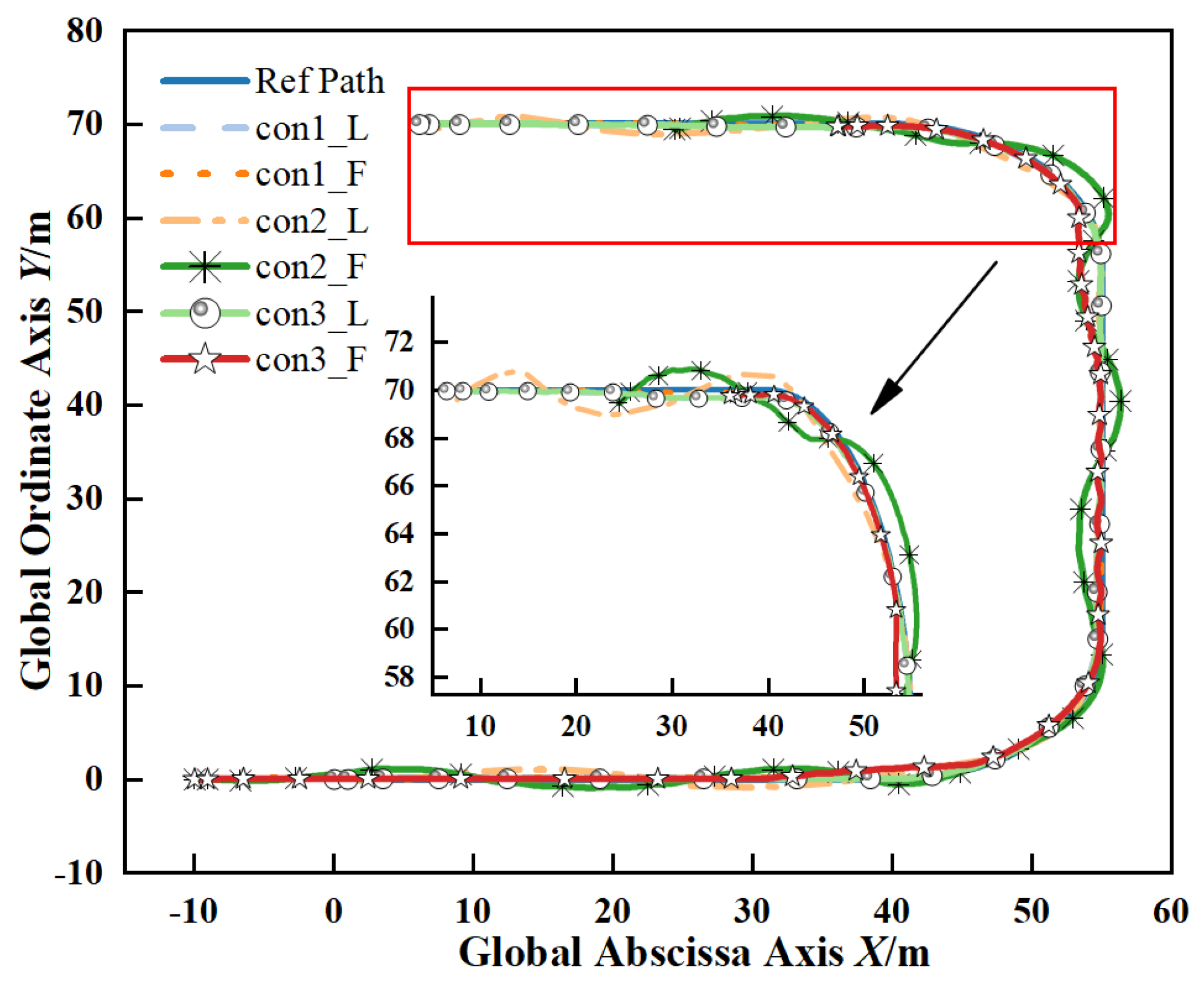
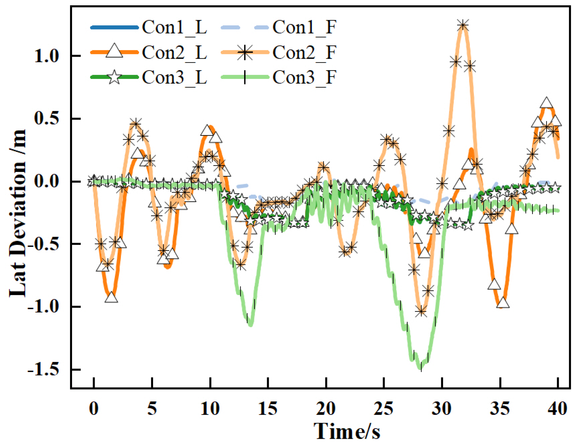
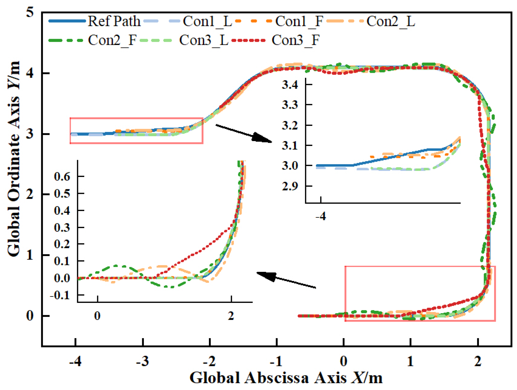
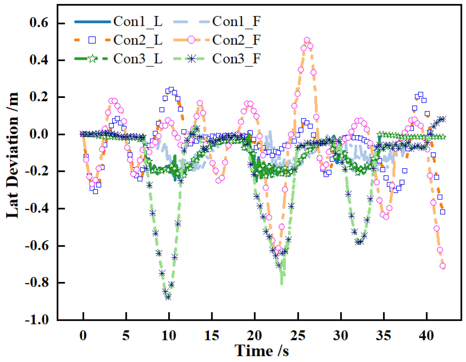
Figure 13 depicts the trajectories of the formation AGVs under different control schemes, where Con1_L and Con1_F denote the leader and follower paths under the proposed method, respectively. The same naming convention applies to other schemes.

The results verify the performance of the three control schemes. Con1 achieves stable motion and accurate path tracking throughout the route, and the proposed formation model adaptively adjusts vehicle spacing such that the AGVs maintain aligned straight-line motion from 0 to 40 m with overlapping trajectories during curve negotiation. Con2 performs significantly worse: its trajectories exhibit pronounced fluctuations between 10 and 40 m on straight segments, with vibration amplitude increasing until the second curve ends, and the follower AGVs generate distinct S-shaped offsets between the two curves because this scheme lacks effective disturbance rejection and error correction, while weak formation control allows the leader’s tracking errors to propagate and amplify among followers until formation stability is recovered during the parking phase. Con3 demonstrates overall smooth performance with consistent trajectories and minor deviations near curves, exhibiting basic robustness with small overshoots; however, its performance degrades in curved sections because it cannot simultaneously handle the coupling of lateral and longitudinal dynamics, reject external disturbances, allocate control outputs, and maintain formation accuracy.

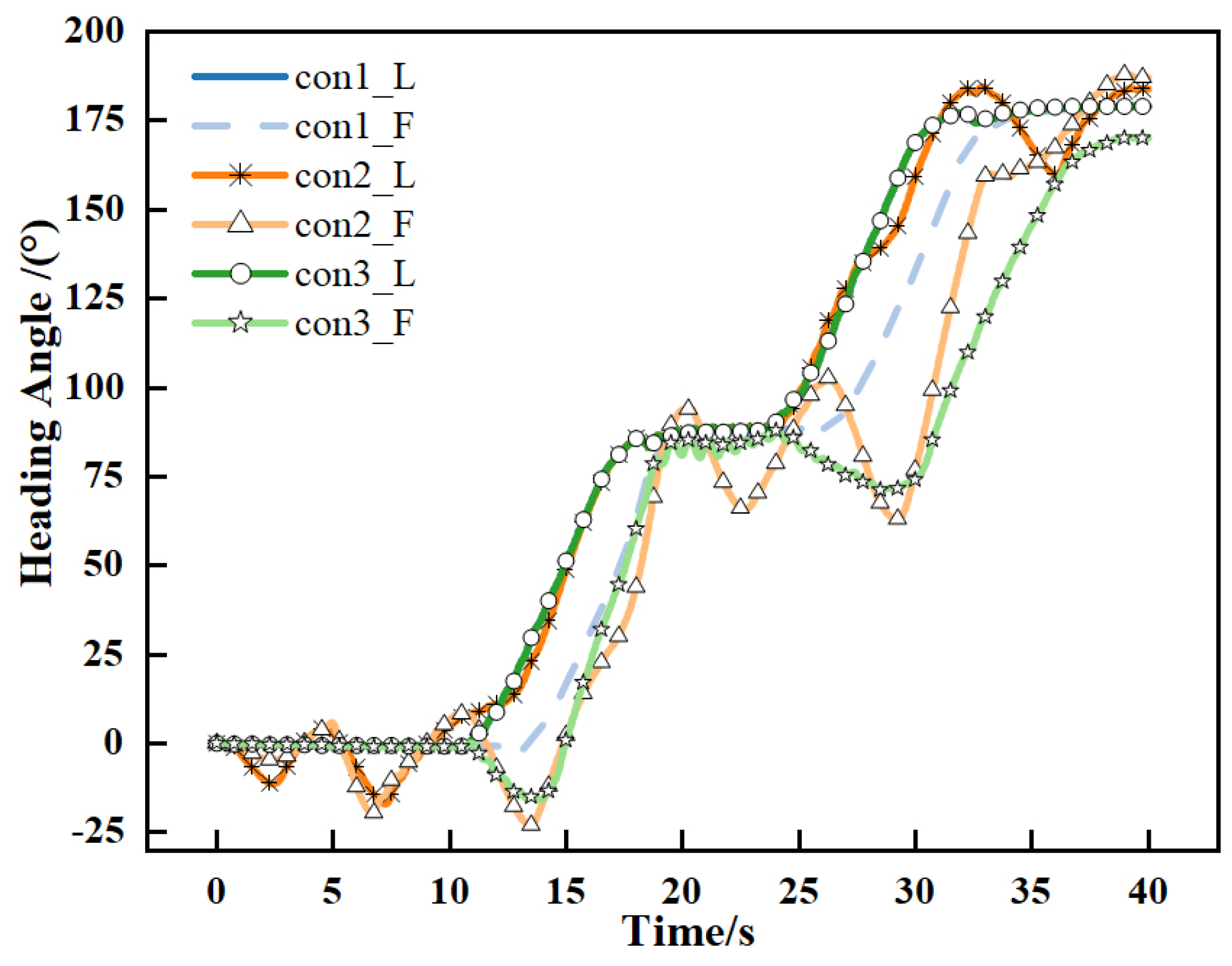
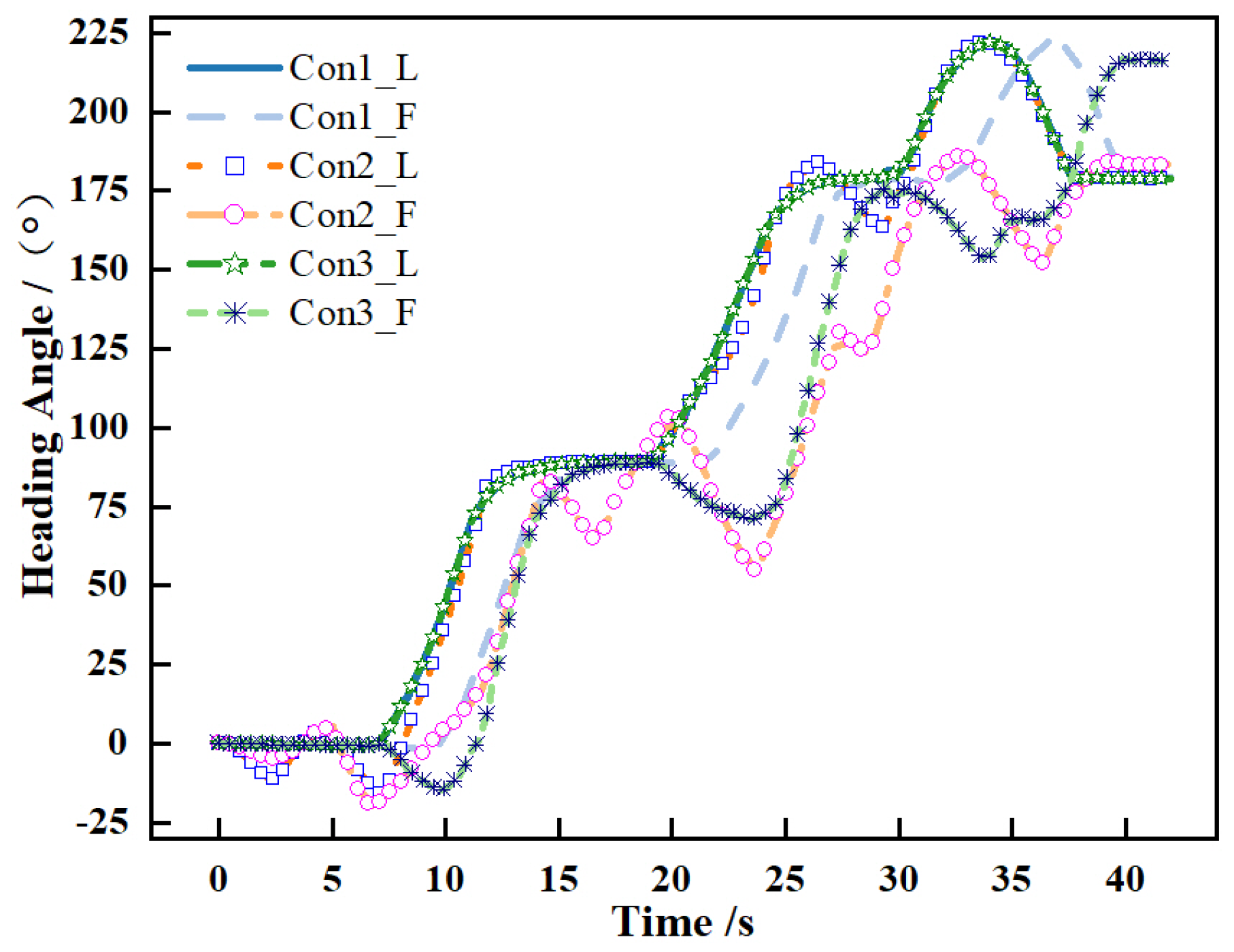
Figure 14 presents the heading angle variations of the formation AGVs. The results show that under Con1, both AGVs exhibit smooth heading transitions with highly consistent trends, demonstrating effective synchronization.

In comparison, Con2 reveals a notable performance disparity: while the leader AGV maintains relatively stable steering with minor heading fluctuations, the follower exhibits significant oscillatory behavior in curved sections, which aligns with the path deviations shown in Figure 13 and confirms the scheme’s limitations in maintaining formation consistency. For Con3, the leader AGV tracks the desired path smoothly with stable heading variations, confirming its capability to resist external disturbances; however, the follower AGV experiences considerable heading fluctuations at the entry phases of both curves, and these errors converge rapidly once the AGVs fully enter the curves, indicating strong system robustness but revealing limitations in handling transient coupling effects and maintaining string stability during formation maneuvers.

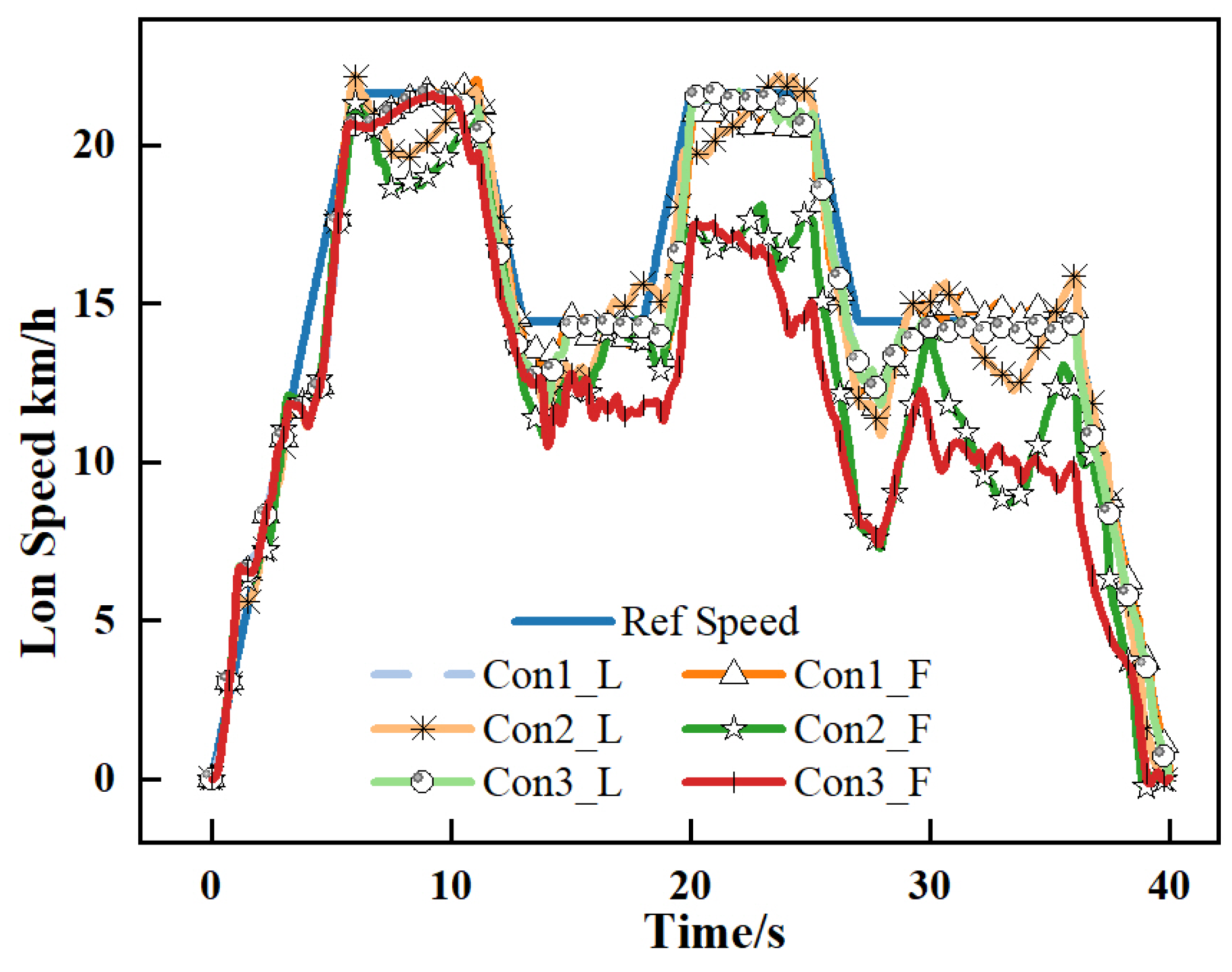
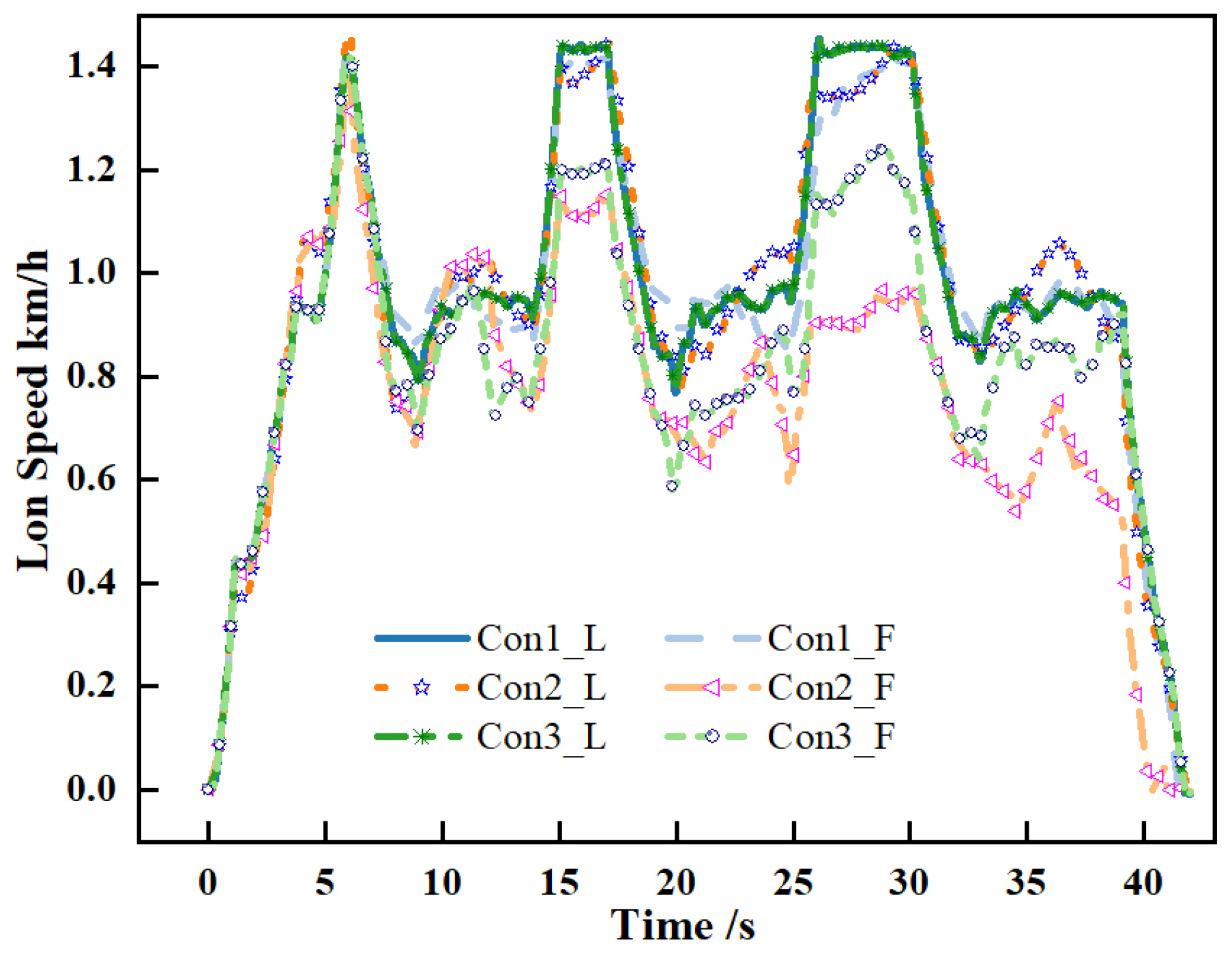
Figure 15 illustrates the longitudinal velocity profiles of the formation AGVs under different control schemes. The results demonstrate that Con1 achieves high velocity synchronization between the AGVs, with only minor fluctuations observed in the follower’s velocity during curve negotiation. This performance confirms the strong responsiveness and disturbance rejection capability of the NTSMC controller. The velocity discrepancies during turning result from the adaptive spacing adjustment in the improved formation model, which introduces acceptable levels of system chattering while maintaining overall controllability.

In contrast, Con2 exhibits substantial velocity errors in curves, while in straight sections, the system attempts to compensate through increased control inputs, leading to noticeable overshoot and unsatisfactory motion smoothness. Similarly, Con3 shows significant velocity synchronization issues during curve negotiation, indicating limited capability in maintaining longitudinal coordination.

Comparative analysis confirms that the proposed Con1 scheme delivers superior performance in longitudinal motion control. Notably, all schemes exhibit stepped velocity profiles during initial acceleration rather than linear increases, attributed to the large AGV mass and inherent system inertia. This observation underscores the importance of high controller responsiveness and rapid error convergence to mitigate inertial effects in heavy-duty AGV applications.

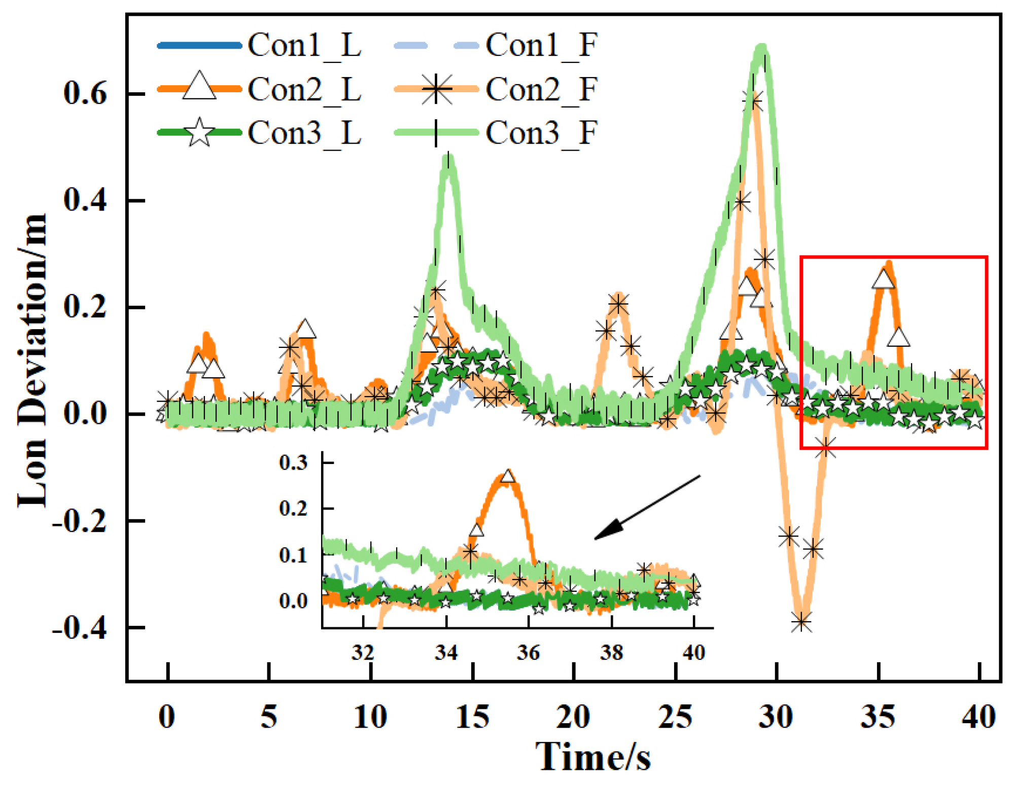
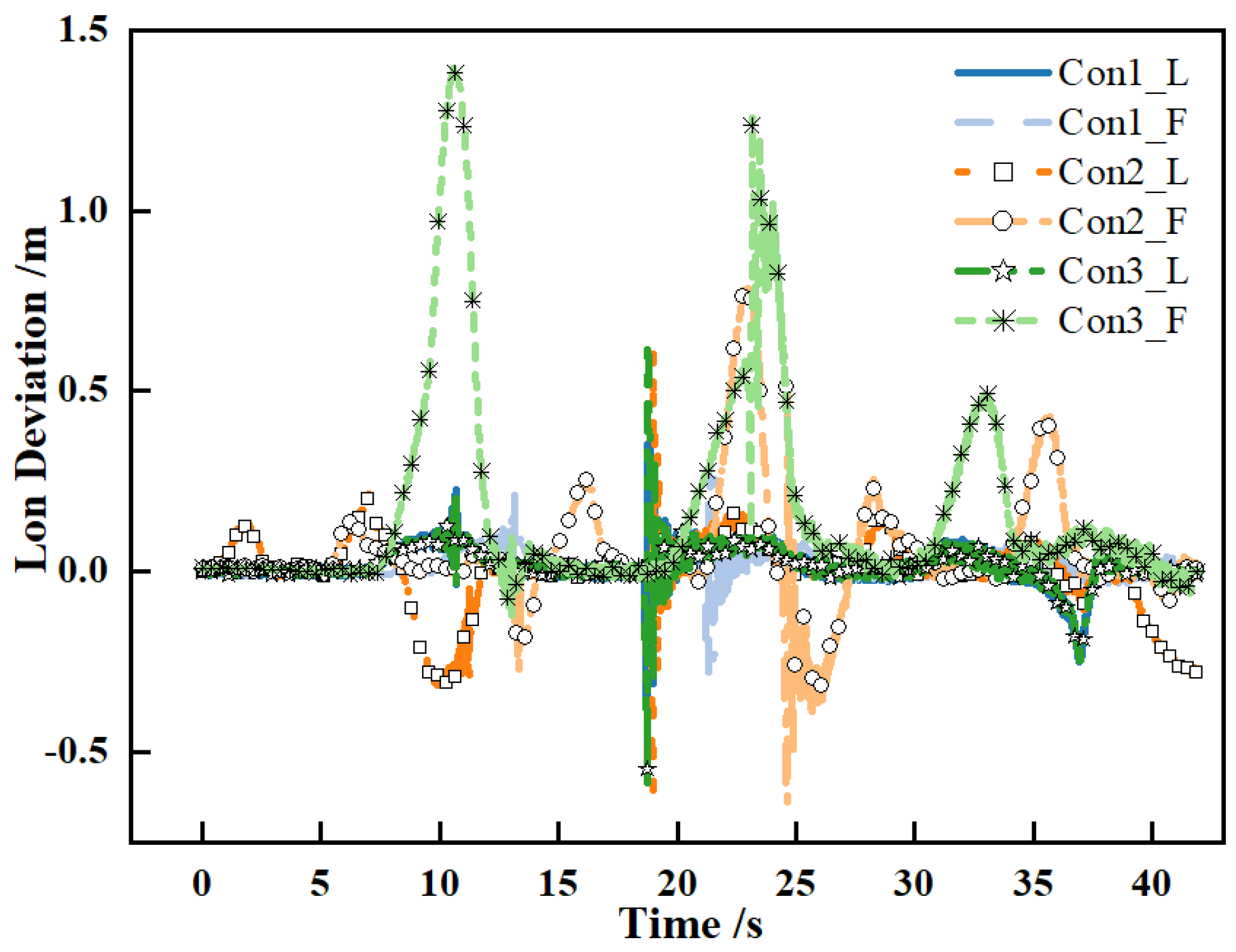
Figure 16 presents the longitudinal tracking errors of the formation AGVs. Under Con1, the formation achieves a steady-state error of 0.018 m, with maximum errors of 0.08 m and 0.092 m in the first and second curves, respectively. The final error at the loading point reaches 0.014 m, demonstrating high precision.

In comparison, Con2 exhibits more frequent error fluctuations, with a steady-state error of 0.032 m and a maximum error of 0.6 m. The final docking error is 0.043 m, indicating inferior stability and precision retention relative to Con1. For Con3, longitudinal errors primarily concentrate in the curve sections, reaching a maximum of 0.68 m. Although this exceeds Con2’s peak error, Con3 maintains better operational stability and synchronization, with a steady-state error of 0.028 m and a final docking error of 0.038 m. Quantitative analysis confirms that Con1 improves longitudinal formation accuracy by 43.75% and 35.71% compared to Con2 and Con3, respectively. More significantly, the docking precision at loading points is enhanced by 67.44% and 63.16% over the benchmark schemes. These improvements directly contribute to optimized traffic efficiency and reduced alignment time between spreaders and AGVs, ultimately enhancing overall operational throughput.

Figure 17 displays the lateral tracking performance of the formation AGVs. Under Con1, the system maintains high motion accuracy in straight segments, with lateral errors converging stably near zero. During curve negotiation, lateral errors increase gradually, reaching a maximum of 0.023 m. The average steady-state error remains at 0.013 m, and the final lateral error at the loading point is 0.016 m, well within the ±0.02 m precision requirement for automated port operations.

In contrast, Con2 exhibits frequent lateral error fluctuations with amplitudes up to 2.2 m, reflecting inadequate lateral control capability that compromises operational stability and introduces safety concerns. The scheme yields an average steady-state error of 0.26 m and a final docking error of 0.34 m, failing to meet automated port precision standards. Con3 maintains reasonable overall accuracy with an average steady-state error of 0.12 m, but shows significant lateral deviations in curves, peaking at –1.5 m in the second curve. The final lateral error of 0.24 m at the docking position also falls short of operational requirements. Quantitatively, Con1 improves average lateral accuracy by 95% and 89.17% over Con2 and Con3, respectively. More notably, it enhances docking precision by 95.29% and 93.33% compared to the two benchmark schemes, demonstrating decisive advantages in lateral control performance.

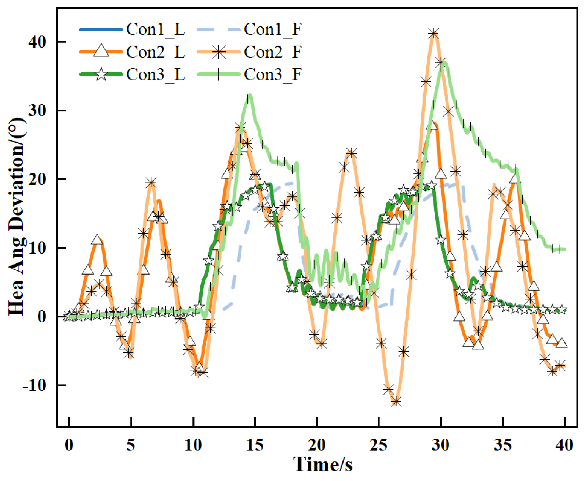
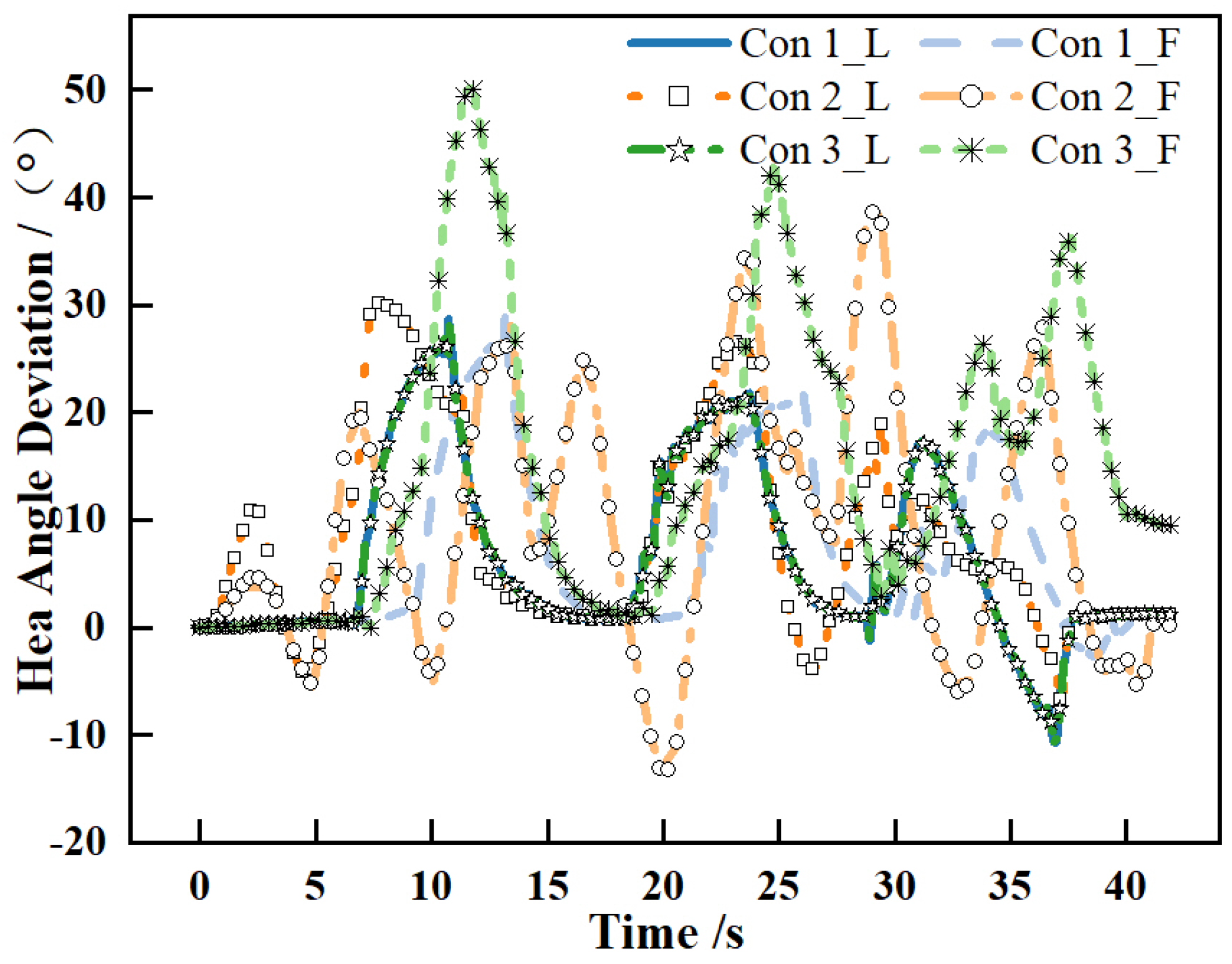
Figure 18 illustrates the heading angle deviations of the formation AGVs under different control schemes. Under Con1, the steady-state heading deviation remains within 1.8°, with slightly larger errors observed during curve negotiation due to the nonholonomic constraints of AGVs. This inherent kinematic limitation creates unreachable regions during turning maneuvers. Nevertheless, the final heading deviation at the loading point is 1.63°, well within the ±2° requirement for automated port operations, ensuring both safety and stability.

In contrast, Con2 exhibits significant heading fluctuations, consistent with its previously observed lateral and longitudinal error patterns. The scheme fails to meet port AGV operational requirements, culminating in a final heading deviation of −7.3° at the docking position. Con3 demonstrates adequate straight-line tracking capability but suffers from insufficient coordinated control in curves, leading to substantial error accumulation. The resulting heading deviation of −8.5° at the loading point further confirms its limitations in formation control. Comparative analysis confirms that Con1 achieves superior lateral motion control, improving heading accuracy at the docking position by 77.67% and 80.82% compared to Con2 and Con3, respectively.

5. Physical Experiment and Analysis

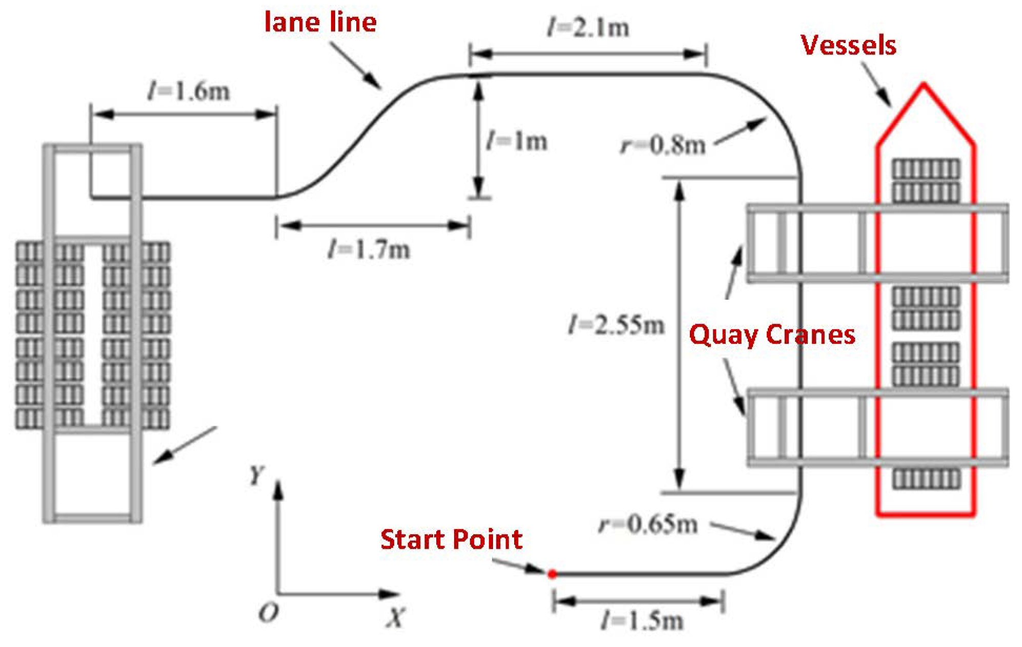
To further verify the engineering applicability of the proposed formation control strategy, verification experiments are conducted on a scaled port AGV test platform in this section. According to field investigation at the port, the travel routes of AGVs for internal transportation mainly consist of straight lines and circular curves. To realistically simulate the actual working environment under existing experimental conditions, a reference path is designed in the test site. Key parameters including segment length and curvature are presented in Figure 19. Restricted by experimental conditions, it is difficult to acquire data such as tire force and slip displacement. Hence, subsequent tests are carried out based on the vehicle kinematic model. This study focuses on evaluating the environmental dependence and practical effectiveness of the proposed strategy. Apart from onboard sensors, six high-speed network cameras are deployed to monitor the real-time operating state of AGVs.

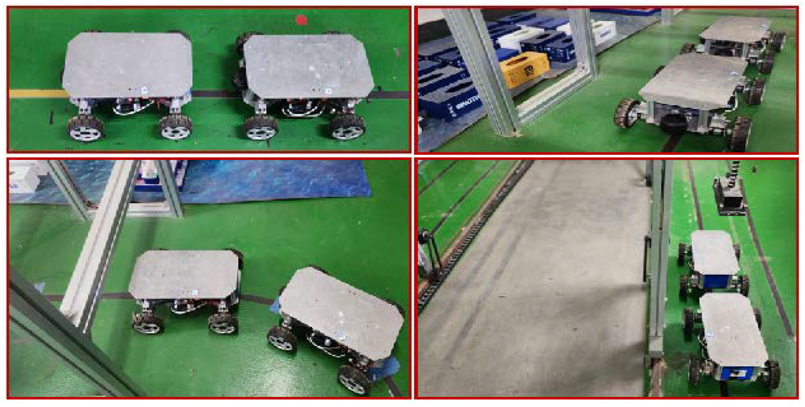
The core hardware of experimental AGV includes Raspberry Pi, STM32, LiDAR, IMU, drive motor, and steering motor. The AGV adopts a master–slave control structure. The Raspberry Pi serves as the main controller for algorithm operation, calculation, and command issuance, while STM32 acts as the slave controller to collect data and execute control commands. The two AGVs share status information via Wi-Fi communication; the core parameters of the AGV are listed in

Table 3. Main parameters of the experimental AGV.

Parameter	Value
Dimensions (L × W × H) /mm	450 × 300 × 200
Curb Weight/kg	10
Vehicle Speed/(m/s)	0–1
Tread/mm	360
Wheelbase/mm	320
Minimum Turning Radius/mm	300

.

Performance tests of dual-AGV formation control are conducted on the port AGV experimental platform. As mentioned above, the unloaded dual-AGV formation moves cooperatively from the quay crane waiting area to the yard loading and unloading area starting from static status, as illustrated in Figure 19. The initial poses of the leading and following AGVs are (−0.81, 0, 0) and (0, 0, $\pi$/12), respectively. The relevant test scenario is presented in Figure 20.

To comprehensively evaluate the overall performance of the proposed formation control strategy for unloaded dual-AGVs, comparative experiments are carried out with two existing strategies, namely, the robust adaptive terminal sliding mode formation control method [57] and the extended-state-observer-based adaptive sliding mode control method [58]. For convenient result analysis, the proposed strategy is denoted as Con1, the strategy in Reference [57] as Con2, and the strategy in Reference [58] as Con3. Con1_L represents the state of the leader AGV under the proposed strategy, and Con2_F refers to the state of the follower AGV adopting the strategy in Reference [57]. Other symbols follow the same naming rule and will not be elaborated hereinafter. The parameter settings of each control scheme are listed as follows:

In Con1, the gain matrix of FT-NDO is set to $l(\Gamma )={[12,4.35;2.18,5.5]}^{\mathrm{T}}$, $\kappa =1.05$, $\alpha =0.28$; the key parameter of lateral SMC is $c_0=1.73$, $c_1=0.12$, $k_s=146$, $k_{\epsilon }=1.77$; the core parameter of longitudinal NTSMC is $k_{\alpha }=0.04$, $k_{\beta }=1.17$. In Con2, the gain matrix of the robust adaptive terminal sliding mode controller is $k_2=\mathrm{diag}(0.13,0.18)$, $k_3=\mathrm{diag}(6.5,7.7)$, and other gain coefficients are $c_1=c_2=0.01$, ${\sigma }_1=2.5$, ${\sigma }_2=0.52$, $\nu =0.45$, ${\varsigma }_1=0.5$. In Con3, the main parameter of the model predictive controller is $N_p=N_c=10$, $Q=3000$, $R=500$. The core parameter of the extended state observer is $k_{z1}=\mathrm{diag}(-13,-13)$, $k_{z2}=\mathrm{diag}(-200,-200)$. The adaptive rates of the sliding mode control gain matrices are ${\gamma }_1={\gamma }_2=0.23$ and ${\varsigma }_1={\varsigma }_2=0.15$. At the start of the test, lateral and longitudinal disturbances $d_1=2\sin \left(10t\right)$, $d_2=5\cos \left(t\right)$ are imposed on the leader and follower AGVs. The detailed experimental results are shown in Figure 21, Figure 22, Figure 23, Figure 24, Figure 25 and Figure 26.

Figure 21 shows that Con1 ensures high motion accuracy and smoothness of AGV formation. Given the limited space in port operation areas, dynamic spacing adjustment reduces turning radius and improves maneuverability. The paths of leader and follower AGVs fit closely, and the formation turning radius equals that of a single vehicle. Con2 maintains good accuracy on straight roads, yet deviation rises notably in curves. The follower AGV suffers severe oscillation and travels along an S-shaped path. Insufficient anti-interference performance causes error backward propagation, enlarging the follower deviation. Con3 enables stable path tracking but brings large steady-state errors. Its disturbance compensation suppresses oscillation and overshoot, while its control accuracy and error convergence rate are inferior to those of Con1.

Figure 22 illustrates heading angle variations under different controllers. Con1 yields the smoothest curve, reflecting stable running state. The follower AGV in Con2 suffers drastic heading fluctuation at curves, while Con3 presents mild fluctuation. The control effect conforms to the above data trend.

Figure 23 indicates Con1 achieves high longitudinal velocity consistency, with maximum error only 0.02 m/s, ensuring safe and efficient formation travel. Con2 generates large velocity deviation from the first bend, peaking at 0.11 m/s, which reflects weak anti-interference capability and hidden safety hazards. Con3 has similar performance but milder velocity oscillation. Its disturbance observer restrains external interference and suppresses backward propagation of formation errors.

Figure 24 shows lateral error curves under different control schemes. Con1 achieves optimal lateral precision, with maximum error −0.25 m, and steady-state error 0.023 m and 0.016 m at loading and unloading positions. The other two schemes fail to maintain low steady-state errors and cannot satisfy operational accuracy demands.

Figure 25 shows Con1 has maximum longitudinal error of −0.18 m, and steady-state error of 0.22 m and 0.013 m at loading-unloading points, effectively shortening alignment time. The other two schemes suffer large non-convergent errors, matching simulation outcomes.

Figure 26 shows Con1 boasts the minimum heading angle error, whose peak value emerges in curves. Driven by the improved formation model, the follower follows the leader’s path to cut the turning radius, causing partial heading deviation. The error at loading-unloading points complies with port attitude precision standards. The other two schemes have prominent attitude errors and fail to meet stability and accuracy demands.

6. Conclusions

6.1. Main Research Outcomes

To address the challenges of limited maneuverability, insufficient docking accuracy, and inadequate disturbance rejection in AGVs operating in complex port environments, this paper proposes a robust control strategy for dual-AGV unloaded formations. The proposed approach is realized through the following key components:

First, based on a leader–follower formation framework, the inter-vehicle spacing is dynamically adjusted according to path curvature, effectively reducing the formation’s turning radius. Second, the dual-AGV formation control task is decoupled into individual trajectory tracking problems for each AGV. A hierarchical control architecture is adopted to address the lateral–longitudinal coupling dynamics, wherein a lateral SMC based on angle parameters and a longitudinal NTSMC are designed to meet the accuracy and real-time requirements of formation control. Third, to further enhance system robustness, an FT-NDO is developed and integrated into both lateral and longitudinal control subsystems.

Simulation and physical experiment results show that the proposed disturbance observer achieves over 95% estimation accuracy, and the overall strategy significantly improves docking pose accuracy compared to existing methods. These findings verify that the proposed approach satisfies the stringent requirements for high-precision formation operation in automated ports under complex disturbance conditions.

6.2. Limitations and Extended Future Research Directions

Although the proposed hierarchical control scheme exhibits satisfactory tracking accuracy and anti-disturbance performance under the given port working conditions, the research still contains several inherent constraints that restrict its universal applicability. The specific limitations and corresponding improvement schemes are analyzed as follows:

(1)

All simulation and physical experiments adopt a fixed AGV mass without comparative tests under variable loaded container conditions. Mass variation changes vehicle inertia and tire vertical loads, which may weaken disturbance estimation and tracking precision.

(2)

Verification only covers a fixed range of road curvatures and a single set of dynamic spacing adjustment thresholds; comparative tests with extreme curve radii and multiple safe spacing boundaries are not conducted.

(3)

Only low-frequency periodic disturbances with fixed amplitudes are adopted in tests, without exploring transient shock interference and disturbance signals of different magnitudes.

(4)

The study only focuses on dual-AGV coordination, while multi-vehicle platoons with communication delay and packet loss are not considered.

To overcome these limitations, we outline comprehensive follow-up research plans: First, we will design an adaptive gain tuning rule for the FT-NDO and sliding mode controllers to accommodate time-varying vehicle loads. Second, systematic comparative experiments with diversified curvatures, adjustable formation spacings, and multi-amplitude disturbances will be performed to fully test the generalization ability of the algorithm. Third, communication delay compensation terms will be embedded into the control loop to extend the method to large AGV platoons. Furthermore, the decoupled anti-disturbance control framework proposed in this paper can be generalized to mixed traffic scenes of automated container terminals, providing technical support for high-efficiency collaborative horizontal transportation in large-scale smart port logistics systems.

References

1. Bruzzone, A.; Giulianetti, A.; Gotelli, M.; Sciomachen, A. The impact of import container flow characteristics on port operational efficiency. Simul. Model. Pract. Theory 2025, 146, 103228. [Google Scholar] [CrossRef] [Scilit]
2. Pourmohammad-Zia, N.; Schulte, F.; González-Ramírez, R.G.; Voß, S.; Negenborn, R.R. A robust optimization approach for platooning of automated ground vehicles in port hinterland corridors. Comput. Ind. Eng. 2023, 177, 109046. [Google Scholar] [CrossRef] [Scilit]
3. Sun, P.Z.; You, J.; Qiu, S.; Wu, E.Q.; Xiong, P.; Song, A.; Zhang, H.; Lu, T. AGV-based vehicle transportation in automated container terminals: A survey. IEEE Trans. Intell. Transp. Syst. 2022, 24, 341–356. [Google Scholar] [CrossRef] [Scilit]
4. Zhang, Q.; Li, W.; Cai, L.; Guo, L.; Qi, X. A Rigid Body Consensus-Based Collaborative Control Framework for Dual AGVs in Smart Port. IEEE Internet Things J. 2025, 12, 25182–25196. [Google Scholar] [CrossRef] [Scilit]
5. Gelareh, S.; Merzouki, R.; McGinley, K.; Murray, R. Scheduling of intelligent and autonomous vehicles under pairing/unpairing collaboration strategy in container terminals. Transp. Res. Part C-Emerg. Technol. 2013, 33, 1–21. [Google Scholar] [CrossRef] [Scilit]
6. Rizzo, C.; Lagraña, A.; Serrano, D. Geomove: Detached agvs for cooperative transportation of large and heavy loads in the aeronautic industry. In Proceedings of the 2020 IEEE International Conference on Autonomous Robot Systems and Competitions (ICARSC), Ponta Delgada, Portugal, 15–17 April 2020; IEEE: Piscataway, NJ, USA, 2020; pp. 126–133. [Google Scholar]
7. Wu, Q.; Wang, X.; Qiu, X. Embedded technique-based formation control of multiple wheeled mobile robots with application to cooperative transportation. Control Eng. Pract. 2024, 150, 106002. [Google Scholar] [CrossRef] [Scilit]
8. Li, J.; Hua, Y.; Yu, J.; Dong, X.; Feng, Z.; Ren, Z. Resilient time-varying formation tracking control for general linear multiagent systems with a nonautonomous leader and adversarial followers. IEEE Trans. Cybern. 2024, 54, 6203–6216. [Google Scholar] [CrossRef] [Scilit] [PubMed]
9. An, S.; Liu, Y.; Wang, X.; Fan, Z.; Zhang, Q.; He, Y.; Wang, L. Distributed Event-Triggered Fixed-Time Leader–Follower Formation Tracking Control of Multiple Underwater Vehicles Based on an Adaptive Fixed-Time Observer. J. Mar. Sci. Eng. 2023, 11, 1522. [Google Scholar]
10. Xu, Z.; Yan, T.; Yang, S.X.; Gadsden, S.A. Distributed leader follower formation control of mobile robots based on bioinspired neural dynamics and adaptive sliding innovation filter. IEEE Trans. Ind. Inform. 2023, 20, 1180–1189. [Google Scholar] [CrossRef] [Scilit]
11. Li, X.; Wang, B.; Wang, Y.; Shi, P.; Zhang, W.; Yan, C. Adaptive switched bipartite time-varying formation control for multiagent systems with inaccessible leader and follower information. IEEE Trans. Syst. Man Cybern. 2026, 56, 3988–4001. [Google Scholar] [CrossRef] [Scilit]
12. Zhang, L.; Li, G.; Liu, R.; Wen, G. Optimized Leader-Follower Formation Fault-Tolerant Control Using Reinforcement Learning for a Class of Nonlinear Multi-Agent Systems Having Actuator Failure. Int. J. Adapt. Control Signal Process. 2025, 39, 2219–2232. [Google Scholar]
13. Fu, L.; Zheng, W.; Wang, H. Nonlinear heterogeneous multi-agent systems under communication switching environment bipartite formation tracking control. Nonlinear Dyn. 2025, 113, 11817–11828. [Google Scholar] [CrossRef] [Scilit]
14. Zhang, Q.; Li, W.; Guo, L.; Qi, X. Collaborative transport strategy for dual AGVs in smart ports: Enhancing docking accuracy in no-load formations. J. Mar. Sci. Eng. 2025, 13, 81. [Google Scholar] [CrossRef] [Scilit]
15. Roque, P.; Miraldo, P.; Dimarogonas, D.V. Multi-agent formation control using epipolar constraints. IEEE Robot. Autom. Lett. 2024, 9, 11002–11009. [Google Scholar] [CrossRef] [Scilit]
16. Verginis, C.K.; Xu, Z.; Topcu, U. Non-parametric neuro-adaptive formation control. IEEE Trans. Autom. Sci. Eng. 2025, 22, 10684–10697. [Google Scholar]
17. He, X.; Luo, D.; Chen, Z.; Yang, G.; Liu, Y. Consensus Based Reinforcement Learning Method for Differentiated Formation Control of UAVs. IEEE Trans. Veh. Technol. 2025, 74, 2429–2442. [Google Scholar] [CrossRef] [Scilit]
18. Hu, M.; Wang, X.; Bian, Y.; Cao, D.; Wang, H. Disturbance observer-based cooperative control of vehicle platoons subject to mismatched disturbance. IEEE Trans. Intell. Veh. 2023, 8, 2748–2758. [Google Scholar] [CrossRef] [Scilit]
19. Guo, G.; Yue, W. Hierarchical platoon control with heterogeneous information feedback. IET Control Theory Appl. 2011, 5, 1766–1781. [Google Scholar] [CrossRef] [Scilit]
20. Li, S.E.; Qin, X.; Li, K.; Wang, J.; Xie, B. Robustness analysis and controller synthesis of homogeneous vehicular platoons with bounded parameter uncertainty. IEEE/ASME Trans. Mechatron. 2017, 22, 1014–1025. [Google Scholar] [CrossRef] [Scilit]
21. Zhang, J.; Liu, X.; Xia, Y.; Zuo, Z.; Wang, Y. Disturbance observer-based integral sliding-mode control for systems with mismatched disturbances. IEEE Trans. Ind. Electron. 2016, 63, 7040–7048. [Google Scholar]
22. Xu, H. Finite-time stability analysis: A tutorial survey. Complexity 2020, 2020, 1941636. [Google Scholar] [CrossRef] [Scilit]
23. Gao, Z.; Guo, G. Fixed-time formation control of AUVs based on a disturbance observer. Acta Autom. Sin. 2019, 45, 1094–1102. [Google Scholar]
24. Zheng, S.; Cui, Y.; Zhao, Q. Disturbance-observer-based adaptive finite-time prescribed performance control for nonlinear systems with input saturation. Int. J. Syst. Sci. 2026, 57, 1239–1251. [Google Scholar]
25. Xu, Z.; Lan, Y.; Lei, C. Fixed-time disturbance observer-based fixed-time prescribed performance control for nonlinear systems with disturbances and full-state constraints. Int. J. Control Autom. Syst. 2024, 22, 2999–3007. [Google Scholar]
26. Sun, X.; Yue, M.; Li, X.; Yu, Z.; Zong, G. Optimal Motion Planning and Decoupled Control for Autonomous Mobile Robots Based on Minimum Energy Consumption. Expert Syst. Appl. 2026, 318, 131995. [Google Scholar] [CrossRef] [Scilit]
27. Guo, G.; Zhang, Q. Finite-time command-filtered lateral-longitudinal formation control of vehicles on rough roads. IEEE Trans. Intell. Veh. 2023, 8, 4331–4340. [Google Scholar] [CrossRef] [Scilit]
28. Mu, D.; Hua, C.; Chen, J.; Li, Y.; Zhang, Y. Fixed-Time Sliding-Mode Lateral-Longitudinal Control for Vehicle Platoon With Strict Lane Constraints and Recoverable Spacing Policy. IEEE Trans. Intell. Transp. Syst. 2025, 26, 14854–14865. [Google Scholar]
29. Guo, L.; Ma, H.; Guan, L.; Guo, P.; Zhao, J.; Wang, J. Hierarchical Lateral-Longitudinal Decoupled Control for Distributed-Drive Intelligent Vehicles Considering Active Front Wheel Steering Compensation. Int. J. Automot. Technol. 2026, 27, 391–412. [Google Scholar]
30. Qiu, M.M.; Wang, Q.; Liu, S.L.; Huang, K.; Wang, Y. Integrated steering and braking control for vehicle trajectory tracking under extreme conditions considering road adhesion coefficient—A dynamic weight coefficient allocation strategy. J. Vib. Control 2026, 10775463261435475. [Google Scholar]
31. Chen, J.; Zhu, B.; Ling, X.; Ruan, X.; Guo, N. A multi-agent reinforcement learning-based approach with lateral-longitudinal coupling for highway on-ramp merging control of autonomous vehicle. Proc. Inst. Mech. Eng. Part D J. Automob. Eng. 2024, 09544070251362075. [Google Scholar]
32. Fan, J.; Yan, P.; Li, R.; Liu, Y.; Wang, F.; Liu, Y.; Chen, C. Decoupled Adaptive Motion Control for Unmanned Tracked Vehicles in the Leader-Following Task. World Electr. Veh. J. 2024, 15, 239. [Google Scholar] [CrossRef] [Scilit]
33. Yu, R.; Zhao, H.; Zhen, S.; Huang, K.; Chen, X.; Sun, H.; Shao, K. A novel trajectory tracking control of AGV based on Udwadia-Kalaba approach. IEEE/CAA J. Autom. Sin. 2016, 11, 1069–1071. [Google Scholar] [CrossRef] [Scilit]
34. Zhang, Z.; Xie, L.; Lu, S.; Wu, X.; Su, H. Vehicle yaw stability control with a two-layered learning MPC. Veh. Syst. Dyn. 2023, 61, 423–444. [Google Scholar]
35. Maleki, M.; Razavi, F.S.; Taghavipour, A. Reinforcement Learning-Based Adaptive Gain Tuning of Terminal Super-Twisting SMC for Lane-Change Control in Autonomous Vehicles. IEEE Access 2025, 13, 197206–197218. [Google Scholar]
36. Liu, Z.; Gong, Q.; Hu, X.; Zhu, G.; Guo, S.; Ma, B.; Li, X. Practical fixed-time formation control with disturbance rejection for marine vehicles under input saturation. ISA Trans. 2025, 164, 100–115. [Google Scholar] [CrossRef] [Scilit] [PubMed]
37. Chen, Y.; Huang, J.; Niu, F.; Dai, X.; Huang, H. Robust predefined fixed-time formation-containment control for multiple unmanned surface vehicles with input saturation. ISA Trans. 2025, 165, 241–253. [Google Scholar] [CrossRef] [Scilit] [PubMed]
38. Zhang, K.; Zhang, W.; Wu, Q.; Du, X. Adaptive fixed-time disturbance observer-based anti-saturation distributed sliding mode formation tracking control for multi-underactuated AUVs under lumped disturbances. Ocean Eng. 2025, 339, 122026. [Google Scholar] [CrossRef] [Scilit]
39. Wang, P.; Yu, C.; Pan, Y.J. Finite-time output feedback cooperative formation control for marine surface vessels with unknown actuator faults. IEEE Trans. Control Netw. Syst. 2022, 10, 887–899. [Google Scholar] [CrossRef] [Scilit]
40. Sui, B.; Liu, Y.; Zhang, J.; Liu, Z.; Zhang, Y. Prescribed-Time Trajectory Tracking Control for Unmanned Surface Vessels with Prescribed Performance Considering Marine Environmental Interferences and Unmodeled Dynamics. J. Mar. Sci. Eng. 2024, 12, 1380. [Google Scholar] [CrossRef] [Scilit]
41. Li, Z.; Lei, K. Robust fixed-time fault-tolerant control for USV with prescribed tracking performance. J. Mar. Sci. Eng. 2024, 12, 799. [Google Scholar] [CrossRef] [Scilit]
42. Zhou, X.; Tian, X.; Liu, H.; Mai, Q. Predefined-Time Cooperative Formation Control of Multiple Underactuated Unmanned Surface Vessels With Smooth Switching Topology. Int. J. Robust Nonlinear Control 2025, 35, 6051–6070. [Google Scholar]
43. Huzaefa, F.; Liu, Y.C. Force distribution and estimation for cooperative transportation control on multiple unmanned ground vehicles. IEEE Trans. Cybern. 2021, 53, 1335–1347. [Google Scholar] [CrossRef] [Scilit]
44. Wang, H.; Peng, L.M.; Wei, Z.; Yang, K.; Jiang, L.; Hashemi, E. A holistic robust motion control framework for autonomous platooning. IEEE Trans. Veh. Technol. 2023, 72, 15213–15226. [Google Scholar] [CrossRef] [Scilit]
45. Li, W.; Zhang, Q.; Zhong, Z.; Guo, L. Lateral and longitudinal hierarchical control of port AGV considering coupling characteristics. J. Mech. Eng. 2025, 61, 383–396. [Google Scholar] [CrossRef] [Scilit]
46. Lee, J.; Hwang, Y.; Choi, S.B. Robust tube-MPC based steering and braking control for path tracking at high-speed driving. IEEE Trans. Veh. Technol. 2023, 72, 15301–15316. [Google Scholar] [CrossRef] [Scilit]
47. Zhang, F.; Zhou, M.; Qi, L. Distributed and coordinated model predictive control for channel resource allocation in cooperative vehicle safety systems. IEEE Internet Things J. 2023, 11, 19328–19343. [Google Scholar] [CrossRef] [Scilit]
48. Bian, Q.; Miao, Q.; Yu, Z.; Tang, T.; Ma, H. Nonlinear acceleration disturbance observer to reject transient peak disturbances for an inertial stabilization-tracking platform. ISA Trans. 2025, 160, 237–247. [Google Scholar] [CrossRef] [Scilit] [PubMed]
49. Wang, Y.; Liu, Y.; Wang, Y.; Chai, T. Neural output feedback control of automobile steer-by-wire system with predefined performance and composite learning. IEEE Trans. Veh. Technol. 2023, 72, 5906–5921. [Google Scholar]
50. Wang, Z.; Sheng, S. Finite time disturbance observer-based adaptive composite control for disturbed unmanned helicopter. ISA Trans. 2025, 163, 139–150. [Google Scholar] [CrossRef] [Scilit] [PubMed]
51. Kim, G.; You, S.; Lee, S.; Shin, D.; Kim, W. Robust nonlinear torque control using steering wheel torque model for electric power steering system. IEEE Trans. Veh. Technol. 2023, 72, 9555–9560. [Google Scholar] [CrossRef] [Scilit]
52. Wang, D.; Kong, M.; Zhang, G.; Liang, X. Adaptive second-order fast terminal sliding-mode formation control for unmanned surface vehicles. J. Mar. Sci. Eng. 2022, 10, 1782. [Google Scholar]
53. Luo, W.; Liu, S. Disturbance observer based nonsingular fast terminal sliding mode control of underactuated AUV. Ocean Eng. 2023, 279, 114553. [Google Scholar] [CrossRef] [Scilit]
54. Fei, J.; Wang, J. Self-Organizing Chebyshev Fuzzy Neural Network Integral Terminal Sliding Mode Control of Active Power Filter. IEEE Internet Things J. 2024, 11, 26291–26303. [Google Scholar] [CrossRef] [Scilit]
55. Peng, W.; Shi, Y.; Zhang, M.; Li, C.; Shang, F.; Li, Z. Fixed time trajectory tracking control for Marine crane with anti-saturation input and unmatched disturbances. Mech. Syst. Signal Proc. 2025, 240, 113378. [Google Scholar] [CrossRef] [Scilit]
56. Li, Z.; Ma, X.; Li, Y. Nonlinear partially saturated control of a double pendulum offshore crane based on fractional-order disturbance observer. Autom. Constr. 2022, 137, 104212. [Google Scholar] [CrossRef] [Scilit]
57. Feng, X.; Wang, C. Robust adaptive terminal sliding mode control of an omnidirectional mobile robot for aircraft skin inspection. Int. J. Control Autom. Syst. 2021, 19, 1078–1088. [Google Scholar]
58. Wang, D.; Wei, W.; Wang, X.; Gao, Y.; Li, Y.; Yu, Q.; Fan, Z. Formation control of multiple mecanum-wheeled mobile robots with physical constraints and uncertainties. Appl. Intell. 2022, 52, 2510–2529. [Google Scholar]
Figure 1. Leader–follower formation model.
Jmse 14 01166 g001
Figure 2. Lateral dynamics model of a dual-axle steering AGV.
Jmse 14 01166 g002
Figure 3. Schematic of the dynamic formation spacing adjustment principle.
Jmse 14 01166 g003
Figure 4. Block diagram of robust control system for dual AGV no-load formation.
Jmse 14 01166 g004
Figure 5. Lateral disturbance and its observation value.
Jmse 14 01166 g005
Figure 6. Longitudinal disturbance and its observation value.
Jmse 14 01166 g006
Figure 7. Box plot of external disturbance estimation errors.
Jmse 14 01166 g007
Figure 8. Operation paths of formation AGVs in an external disturbance environment.
Jmse 14 01166 g008
Figure 9. The wheel steering angle of formation AGVs without the participation of an observer.
Jmse 14 01166 g009
Figure 10. The wheel steering angle of formation AGVs with the participation of an observer.
Jmse 14 01166 g010
Figure 11. Heading angle curves of formation under external disturbances.
Jmse 14 01166 g011
Figure 12. Velocity curves of formation under external disturbances.
Jmse 14 01166 g012
Figure 13. Operation paths of formation AGVs under different control schemes.
Jmse 14 01166 g013
Figure 14. Heading angle curves of formation AGVs.
Jmse 14 01166 g014
Figure 15. Longitudinal velocity curves of formation AGVs.
Jmse 14 01166 g015
Figure 16. Longitudinal error curves of formation AGVs.
Jmse 14 01166 g016
Figure 17. Lateral error curves of formation AGVs.
Jmse 14 01166 g017
Figure 18. Heading angle error curves of formation AGVs.
Jmse 14 01166 g018
Figure 19. Reference path of port AGV formation control experimental platform.
Jmse 14 01166 g019
Figure 20. Experimental scene of dual-AGV formation control.
Jmse 14 01166 g020
Figure 21. Path curve of formation AGV in platform experiment.
Jmse 14 01166 g021
Figure 22. Heading angle curve of formation AGV on experimental platform.
Jmse 14 01166 g022
Figure 23. Velocity curve of formation AGV on experimental platform.
Jmse 14 01166 g023
Figure 24. Lateral error curve of formation AGV on experimental platform.
Jmse 14 01166 g024
Figure 25. Longitudinal error of formation AGV on experimental platform.
Jmse 14 01166 g025
Figure 26. Heading angle error of formation AGV on experimental platform.
Jmse 14 01166 g026