A Robust Two-Dimensional Shallow Flow Model with Adaptive Quadtree Mesh

Abstract

A two-dimensional shallow flow model is developed by integrating a positivity-preserving, well-balanced central-upwind scheme with a block-structured quadtree AMR grid implemented in the Afivo open-source framework. A non-negative water depth reconstruction ensures second-order spatial accuracy and the robust treatment of wetting and drying, while coarse-grid fluxes at refinement boundaries are obtained by summing the corresponding fine-grid fluxes, thereby guaranteeing strict mass conservation between refinement levels. Mesh refinement is driven by gradients in water surface elevation, which focus resolution on regions of rapid flow variation, thereby improving both accuracy and computational efficiency. Model validation through benchmark problems and the Malpasset dam-break event show close agreement with analytical solutions, laboratory measurements, and previous numerical simulations, while achieving substantial reductions in computational cost.

1. Introduction

The Saint-Venant system or shallow water equations (SWEs) are fundamental for simulating gravity-driven free-surface flows over irregular terrain. They are widely used in simulations of fluvial floods [1], dam-break events [2], tsunami propagation [3], and tidal hydrodynamics [4]. Mathematically, the SWEs constitute a nonlinear hyperbolic system of conservation laws. Except for a few simplified cases involving idealized geometries and initial/boundary conditions, analytical solutions are generally unavailable, making numerical methods essential for practical applications.

Extensive research has focused on developing numerical schemes capable of accurately resolving shock waves, preserving physically relevant steady states (e.g., the “lake at rest”), and ensuring non-negativity of water depth. Among them, Godunov-type upwind schemes, such as Roe [5], HLL [6], and HLLC [7], have been widely adopted. These methods solve approximate Riemann problems at cell interfaces, providing strong shock-capturing performance and high accuracy. However, they are computationally intensive and complex to implement, particularly in multidimensional and dynamically evolving domains.

To reduce algorithmic complexity, central schemes such as the Lax–Friedrichs scheme [8,9] have been proposed, offering simpler implementations by avoiding Riemann solvers. However, classical central schemes suffer from excessive numerical dissipation, which can degrade accuracy near sharp gradients. To address this, central-upwind schemes were proposed by Kurganov and Petrova [10], combining the simplicity of central schemes with an upwind nature by considering local one-sided wave speeds. This enhances resolution of discontinuities while maintaining robustness and simplicity. Wu et al. [11] presented a positivity-preserving and well-balanced shallow water model using central-upwind schemes and non-negative reconstruction. The model successfully resolved wet/dry fronts over complex terrain while conserving mass and maintaining numerical stability. Furthermore, according to Ginting and Mundani [12], central-upwind schemes outperform HLLC and Roe schemes in efficiency, being roughly 1.4 and 1.25 times faster, respectively, at equivalent accuracy. These advantages make central-upwind schemes well-suited for efficient and robust shallow water modeling.

Beyond numerical schemes, the underlying grid structure significantly influences model performance. Cartesian grids are favored for their simplicity and compatibility with finite volume methods. Many established models employ uniform Cartesian meshes with reliable results across diverse scenarios [13,14,15,16]. However, their inability to conform to complex geometries—such as curved coastlines or variable terrain—can introduce geometric errors and spurious oscillations. Unstructured grids, especially triangular ones, offer improved geometric flexibility and support local refinement, but at the cost of increased complexity in data structures and flux computations. As a compromise, quadtree grids hierarchically refine Cartesian cells, enabling local adaptivity while preserving structured grid benefits, making them attractive for efficient and accurate modeling in irregular domains.

To enhance spatial adaptivity, quadtree-based adaptive mesh refinement (AMR) has proven effective in shallow water modeling. AMR refines the grid dynamically in regions with complex flow features, such as shocks, wetting/drying fronts, or steep topography, while coarsening elsewhere to optimize efficiency. The GeoClaw framework [17] demonstrated AMR’s effectiveness in tsunami and flood modeling. The research group of Liang conducted a series of studies on quadtree-based AMR for shallow water modeling, demonstrating its effectiveness in improving flood simulation accuracy and efficiency over complex terrain [18,19,20]. Using the Basilisk software (http://basilisk.fr/ accessded on 16 September 2025), Kirstetter et al. [21] developed the B-Flood model to successfully reproduce the 2015 Cannes flash flood. More recently, Kyanjo et al. [22] introduced GeoFlood, an open-source SWE solver based on ForestClaw [23], which employs parallel quadtree AMR to support high-resolution and scalable hydrodynamic simulations.

In this study, we extend our previous shallow water model [11], a central-upwind scheme on Cartesian grids designed to prevent negative water depths and preserve well-balanced property, into a quadtree-based adaptive mesh refinement (AMR) framework using Afivo [24]. Afivo is an open-source, Fortran-based AMR library that supports shared-memory parallelism (OpenMP), efficient ghost-cell handling, and a built-in multigrid solver. Although it does not include physical solvers, its modular design makes it easy to implement custom numerical methods. By integrating our model into Afivo’s AMR structure, we maintain key features like well-balanced and mass conservation while improving computational efficiency and local resolution. This enables higher accuracy and improved scalability in simulating shallow water dynamics over irregular terrain.

2. Model Description

2.1. Governing Equations

The conservative formulation of the two-dimensional shallow water equations (SWEs) is derived by depth-integrating the three-dimensional Navier-Stokes system under the hydrostatic pressure assumption:

$${\displaystyle \frac{\partial \mathbf{U}}{\partial t}}+{\displaystyle \frac{\partial \mathbf{C}\left(\mathbf{U}\right)}{\partial x}}+{\displaystyle \frac{\partial \mathbf{D}\left(\mathbf{U}\right)}{\partial y}}=\mathbf{S}\left(\mathbf{U}\right),$$

(1)

where t denotes time, and $(x,y)$ denote the horizontal spatial coordinates.

$\mathbf{U}$ is the vector of conserved variables, given by

$$\mathbf{U}=\left[\begin{array}{c}\eta \\ hu\\ hv\end{array}\right],$$

(2)

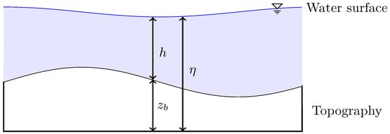
where h is the water depth, $z_b(x,y)$ is the bed elevation, $\eta =h+z_b$ denotes the water surface (Figure 1), and $u,v$ are the depth-averaged velocities in the x- and y-directions, respectively.

Figure 1. Schematic illustration of the relationship between water surface $\eta$, water depth h, and topographic elevation $z_b$.

The flux vectors in the x- and y-directions are

$$\mathbf{C}\left(\mathbf{U}\right)=\left[\begin{array}{c}hu\\ h{u}^2+{\displaystyle \frac{1}{2}}g{h}^2\\ huv\end{array}\right],\mathbf{D}\left(\mathbf{U}\right)=\left[\begin{array}{c}hv\\ huv\\ h{v}^2+{\displaystyle \frac{1}{2}}g{h}^2\end{array}\right],$$

(3)

where g is the acceleration due to gravity.

$\mathbf{S}$ denotes the source term and is given by

$$\mathbf{S}=\left[\begin{array}{c}0\\ -gh{\displaystyle \frac{\partial z_b}{\partial x}}-g{\displaystyle \frac{u\sqrt{u^2+v^2}{n}^2}{h^{1/3}}}\\ -gh{\displaystyle \frac{\partial z_b}{\partial y}}-g{\displaystyle \frac{v\sqrt{u^2+v^2}{n}^2}{h^{1/3}}}\end{array}\right],$$

(4)

where n denotes the Manning roughness coefficient.

2.2. Numerical Scheme

2.2.1. Finite Volume Method

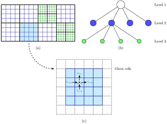
In this model, the shallow water equations are discretized using a finite volume method on the quadtree-based AMR grid described in Section 2.3 (see Figure 2). Although the global mesh is nonuniform due to adaptive refinement, each block locally retains a uniform Cartesian layout, allowing the use of conventional finite volume flux evaluation procedures developed for structured grids.

Figure 2. Schematic representation of the adaptive quadtree grid system used in the model: (a) overall adaptive grid layout; (b) hierarchical tree structure; (c) single block with ghost cells and flux interfaces.

Integrating Equation (1) over the control volume corresponding to cell $(k,l)$ yields the following:

$${\mathbf{U}}_{k,l}^{o+1}={\mathbf{U}}_{k,l}^o-{\displaystyle \frac{\Delta t}{\Delta x}}\left({\mathbf{C}}_{k+{\displaystyle \frac{1}{2}},l}^o-{\mathbf{C}}_{k-{\displaystyle \frac{1}{2}},l}^o\right)-{\displaystyle \frac{\Delta t}{\Delta y}}\left({\mathbf{D}}_{k,l+{\displaystyle \frac{1}{2}}}^o-{\mathbf{D}}_{k,l-{\displaystyle \frac{1}{2}}}^o\right)+\Delta t{\mathbf{S}}_{k,l}^o$$

(5)

Here, the superscript o indicates the time level, while l and k denote the grid indices along the y- and x-axes. The parameters $\Delta t$, $\Delta y$, and $\Delta x$ correspond to the temporal increment and the spatial cell sizes in the y and x directions. The ${\mathbf{C}}_{k\pm {\displaystyle \frac{1}{2}},l}^o$ and ${\mathbf{D}}_{k,l\pm {\displaystyle \frac{1}{2}}}^o$ describe fluxes across vertical and horizontal interfaces.

2.2.2. Non-Negative Water Depth Reconstruction

To preserve the well-balanced property and correctly treat wetting and drying, we employ the non-negative water depth reconstruction technique of Liang [25], which integrates seamlessly with the AMR framework. This approach achieves second-order spatial accuracy while maintaining the C-property.

First, the left Riemann states of the conserved quantities at the eastern interface $(k+\frac{1}{2},l)$ are reconstructed from cell-centered values using slope limiters:

$$\begin{array}{cc}\hfill {\overline{\eta }}_{k+1/2,l}^L& =0.5{\phi }_k({\eta }_{k,l}-{\eta }_{k-1,l})+{\eta }_{k,l}\hfill \end{array}$$

(6)

$$\begin{array}{cc}\hfill {\overline{h}}_{k+1/2,l}^L& =0.5{\phi }_k(h_{k,l}-h_{k-1,l})+h_{k,l}\hfill \end{array}$$

(7)

$$\begin{array}{cc}\hfill {\overline{\left(hu\right)}}_{k+1/2,l}^L& =0.5{\phi }_k({\left(hu\right)}_{k,l}-{\left(hu\right)}_{k-1,l})+{\left(hu\right)}_{k,l}\hfill \end{array}$$

(8)

$$\begin{array}{cc}\hfill {\overline{\left(hv\right)}}_{k+1/2,l}^L& =0.5{\phi }_k({\left(hv\right)}_{k,l}-{\left(hv\right)}_{k-1,l})+{\left(hv\right)}_{k,l}\hfill \end{array}$$

(9)

where ${\phi }_k$ represents a component-wise slope limiter, for which the minmod limiter is adopted in this study.

The interface velocity components are subsequently reconstructed as follows:

$${\overline{u}}_{k+1/2,l}^L={\displaystyle \frac{{\overline{\left(hu\right)}}_{k+1/2,l}^L}{{\overline{h}}_{k+1/2,l}^L}},{\overline{v}}_{k+1/2,l}^L={\displaystyle \frac{{\overline{\left(hv\right)}}_{k+1/2,l}^L}{{\overline{h}}_{k+1/2,l}^L}}$$

(10)

When the reconstructed depth is below a threshold (i.e., $h<{10}^{-8}$), the velocity components are assigned zero to prevent numerical instability.

The corresponding reconstructed bed elevation is then computed as follows:

$${\left(\overline{z_b}\right)}_{k+1/2,l}^L={\overline{\eta }}_{k+1/2,l}^L-{\overline{h}}_{k+1/2,l}^L$$

(11)

The right Riemann states ${\overline{\eta }}_{k+1/2,l}^R$, ${\overline{h}}_{k+1/2,l}^R$, etc., are obtained analogously using the neighboring cells $(k+1,l)$ and $(k+2,l)$.

Following Audusse et al. [26], a unified bed elevation at the interface is introduced as

$${\left(z_b\right)}_{k+1/2,l}=max\left\{{\left(\overline{z_b}\right)}_{k+1/2,l}^L,{\left(\overline{z_b}\right)}_{k+1/2,l}^R\right\}$$

(12)

The water depth values at the interfaces are subsequently adjusted to guarantee non-negativity:

$$\begin{array}{cc}\hfill h_{k+1/2,l}^L& =max\left\{{\overline{\eta }}_{k+1/2,l}^L-{\left(z_b\right)}_{k+1/2,l},0\right\}\hfill \end{array}$$

(13)

$$\begin{array}{cc}\hfill h_{k+1/2,l}^R& =max\left\{{\overline{\eta }}_{k+1/2,l}^R-{\left(z_b\right)}_{k+1/2,l},0\right\}\hfill \end{array}$$

(14)

Using the corrected water depths, the Riemann states are updated as follows:

$$\begin{array}{cc}\hfill {\eta }_{k+1/2,l}^L& =h_{k+1/2,l}^L+{\left(z_b\right)}_{k+1/2,l}\hfill \end{array}$$

(15)

$$\begin{array}{cc}\hfill {\left(hu\right)}_{k+1/2,l}^L& =h_{k+1/2,l}^L·{\overline{u}}_{k+1/2,l}^L\hfill \end{array}$$

(16)

$$\begin{array}{cc}\hfill {\left(hv\right)}_{k+1/2,l}^L& =h_{k+1/2,j}^L·{\overline{v}}_{k+1/2,l}^L\hfill \end{array}$$

(17)

$$\begin{array}{cc}\hfill {\eta }_{k+1/2,l}^R& =h_{k+1/2,l}^R+{\left(z_b\right)}_{k+1/2,l}\hfill \end{array}$$

(18)

$$\begin{array}{cc}\hfill {\left(hu\right)}_{k+1/2,l}^R& =h_{k+1/2,l}^R·{\overline{u}}_{k+1/2,l}^R\hfill \end{array}$$

(19)

$$\begin{array}{cc}\hfill {\left(hv\right)}_{k+1/2,l}^R& =h_{k+1/2,l}^R·{\overline{v}}_{k+1/2,l}^R\hfill \end{array}$$

(20)

Finally, to preserve steady states at wet/dry fronts when the bed elevation of the dry cell exceeds the surface elevation of a neighboring wet cell, the following correction is applied:

$$\Delta z=max\left\{{\left(z_b\right)}_{k+1/2,l}-{\eta }_{k+1/2,l}^L,{\left(z_b\right)}_{k+1/2,l}-{\eta }_{k+1/2,l}^R,0\right\}$$

(21)

$$\begin{array}{cc}\hfill {\left(z_b\right)}_{k+1/2,l}-\Delta z& \to {\left(z_b\right)}_{k+1/2,l}\hfill \\ \hfill {\eta }_{k+1/2,l}^L-\Delta z& \to {\eta }_{k+1/2,l}^L\hfill \\ \hfill {\eta }_{k+1/2,l}^R-\Delta z& \to {\eta }_{k+1/2,l}^R\hfill \end{array}$$

(22)

This approach ensures that, at wet–dry interfaces, the reconstructed free surface and bed elevation coincide with the water surface of the adjacent wet cell, thereby maintaining the scheme’s well-balanced property.

2.2.3. Numerical Fluxes Calculation

The mass and momentum fluxes at interfaces are evaluated using the central-upwind scheme of Kurganov and Petrova [10]. This scheme has been widely applied in shallow water modeling due to its simplicity, robustness, and ability to handle discontinuities and wetting/drying phenomena without solving Riemann problems. The method is particularly well-suited for adaptive grids, as it only requires local estimates of wave speeds and reconstructed Riemann states.

At a vertical interface $(k+\frac{1}{2},l)$ along the x-direction, the flux vector ${\mathbf{C}}_{k+1/2,l}$ is evaluated as follows:

$$\begin{array}{c}\hfill {\mathbf{C}}_{k+1/2,l}={\displaystyle \frac{A_{k+1/2,l}^{+}\mathbf{C}\left({\mathbf{U}}_{k+1/2,l}^L\right)-A_{k+1/2,l}^{-}\mathbf{C}\left({\mathbf{U}}_{k+1/2,l}^R\right)}{A_{k+1/2,l}^{+}-A_{k+1/2,l}^{-}}}\\ \hfill +{\displaystyle \frac{A_{k+1/2,l}^{+}{A}_{k+1/2,l}^{-}}{A_{k+1/2,l}^{+}-A_{k+1/2,l}^{-}}}\left({\mathbf{U}}_{k+1/2,l}^R-{\mathbf{U}}_{k+1/2,l}^L\right)\end{array}$$

(23)

where ${\mathbf{U}}_{k+1/2,l}^L$ and ${\mathbf{U}}_{k+1/2,l}^R$ are the reconstructed left and right Riemann states at the interface, obtained from the non-negative reconstruction procedure described in Section 2.2.2.

The one-sided wave speeds $A_{k+1/2,l}^{+}$ and $A_{k+1/2,l}^{-}$ at the interface are evaluated from the following:

$$\begin{array}{cc}\hfill A_{k+1/2,l}^{+}& =max\left(u_{k+1/2,l}^L+\sqrt{g{h}_{k+1/2,l}^L},u_{k+1/2,l}^R+\sqrt{g{h}_{k+1/2,l}^R},0\right)\hfill \end{array}$$

(24)

$$\begin{array}{cc}\hfill A_{k+1/2,l}^{-}& =min\left(u_{k+1/2,l}^L-\sqrt{g{h}_{k+1/2,l}^L},u_{k+1/2,l}^R-\sqrt{g{h}_{k+1/2,l}^R},0\right)\hfill \end{array}$$

(25)

where $u_{k+1/2,l}^{L,R}$ and $h_{k+1/2,k}^{L,R}$ are the reconstructed velocity components and water depths associated with the left and right states at $(k+\frac{1}{2},l)$, respectively.

A similar procedure is used to compute the flux ${\mathbf{D}}_{k,l+1/2}$ at the horizontal interface $(k,l+{\displaystyle \frac{1}{2}})$ in the y-direction:

$$\begin{array}{c}\hfill {\mathbf{D}}_{k,l+1/2}={\displaystyle \frac{B_{k,l+1/2}^{+}\mathbf{D}\left({\mathbf{U}}_{k,l+1/2}^L\right)-B_{k,l+1/2}^{-}\mathbf{D}\left({\mathbf{U}}_{k,l+1/2}^R\right)}{B_{k,l+1/2}^{+}-B_{k,l+1/2}^{-}}}\\ \hfill +{\displaystyle \frac{B_{k,l+1/2}^{+}{B}_{k,l+1/2}^{-}}{B_{k,l+1/2}^{+}-B_{k,l+1/2}^{-}}}\left({\mathbf{U}}_{k,l+1/2}^R-{\mathbf{U}}_{k,l+1/2}^L\right)\end{array}$$

(26)

The one-sided wave speeds in the y-direction are given by the following:

$$\begin{array}{cc}\hfill B_{k,l+1/2}^{+}& =max\left(v_{k,l+1/2}^L+\sqrt{g{h}_{k,l+1/2}^L},v_{k,l+1/2}^R+\sqrt{g{h}_{k,l+1/2}^R},0\right)\hfill \end{array}$$

(27)

$$\begin{array}{cc}\hfill B_{k,l+1/2}^{-}& =min\left(v_{k,l+1/2}^L-\sqrt{g{h}_{k,l+1/2}^L},v_{k,l+1/2}^R-\sqrt{g{h}_{k,l+1/2}^R},0\right)\hfill \end{array}$$

(28)

where $v_{k,l+1/2}^{L,R}$ and $h_{k,l+1/2}^{L,R}$ are the reconstructed velocities and water depths on the left and right sides of the interface $(k,l+1/2)$, respectively.

2.2.4. Source Terms Treatment

Proper discretization of the source term (see Equation (4)) is vital to ensure that the numerical method remains well-balanced, particularly when modeling stationary flows over uneven topography.

The first component of the source term corresponds to bed slope and is approximated using a central difference scheme that does not require special balancing corrections, owing to the non-negative reconstruction. For instance, in the x-direction the discretization is given by the following:

$${\left(-gh{\displaystyle \frac{\partial z_b}{\partial x}}\right)}_{k,l}=-g{\displaystyle \frac{h_{k+1/2,l}^L+h_{k-1/2,l}^R}{2}}·{\displaystyle \frac{{\left(z_b\right)}_{k+1/2,l}-{\left(z_b\right)}_{k-1/2,l}}{\Delta x}}$$

(29)

Here, $h_{k+1/2,l}^L$ and $h_{k-1/2,l}^R$ denote the reconstructed depths on the left and right sides of the cell interfaces, while ${\left(z_b\right)}_{k\pm 1/2,l}$ are the associated bed elevations. An analogous formulation is used in the y-direction.

The second component of the source term corresponds to bottom friction, a nonlinear contribution dependent on velocity and water depth and commonly represented by the Manning formula. A fully explicit discretization may lead to numerical instabilities in shallow regions due to the singularity of $h^{1/3}$ near dry states. To address this, a semi-implicit strategy is employed, in which the friction term is handled implicitly in the discharge variables, while all other terms remain explicit:

$${\mathbf{S}}_f={\displaystyle \frac{g\sqrt{u^2+v^2}{n}^2}{h^{1/3}}}\left[\begin{array}{c}u\\ v\end{array}\right]={\left({\displaystyle \frac{g{n}^2\sqrt{u^2+v^2}}{h^{4/3}}}\right)}^o\left[\begin{array}{c}{\left(hu\right)}^{o+1}\\ {\left(hv\right)}^{o+1}\end{array}\right]$$

(30)

2.2.5. Model Stability

Within the quadtree-based AMR framework, the spatial resolutions $\Delta x_{k,l}$ and $\Delta y_{k,l}$ vary according to the local refinement level, while the maximum wave propagation speeds in the x- and y-directions at each interface are defined as follows:

$$\begin{array}{cc}\hfill A_{k+1/2,l}& =max\left(A_{k+1/2,l}^{+},-A_{k+1/2,l}^{-}\right),\hfill \end{array}$$

(31)

$$\begin{array}{cc}\hfill B_{k,l+1/2}& =max\left(B_{k,l+1/2}^{+},-B_{k,l+1/2}^{-}\right),\hfill \end{array}$$

(32)

where $A_{k+1/2,l}^{\pm }$ and $B_{k,l+1/2}^{\pm }$ are the one-sided local wave speeds in the x- and y-directions, respectively, as defined in Section 2.2.3.

Because the present scheme is explicit, the time step $\Delta t$ is restricted by the Courant–Friedrichs–Lewy (CFL) condition:

$$\Delta t=Cr\underset{k,l}{min}\left({\displaystyle \frac{\Delta x_{k,l}}{A_{k+1/2,l}}},{\displaystyle \frac{\Delta y_{k,l}}{B_{k,l+1/2}}}\right),$$

(33)

where $Cr$ denotes the Courant number. Following the recommendations of Kurganov and Petrova [10] and Wu et al. [11], $Cr=0.25$ is adopted in all simulations to ensure stability and positivity of water depth.

2.3. Adaptive Mesh

2.3.1. Block-Structured Quadtree Framework

The model utilizes a block-structured quadtree adaptive mesh implemented in the Afivo framework [24], as depicted in Figure 2. Figure 2a illustrates the overall grid organization. The computational domain is partitioned into non-overlapping boxes, which act as the fundamental computational units. Each box consists of $N\times N$ uniformly distributed cells, where N is an even integer. The quadtree structure is straightforward: every box contains the same number of cells, and refinement follows consistent rules. Once refinement is activated, a parent box is divided into four equally sized child boxes, effectively doubling the spatial resolution in both spatial directions.

Figure 2b illustrates the hierarchical quadtree data structure. In this representation, circles denote boxes. White circles correspond to parent boxes, each of which can be split into four child boxes. The hierarchical links between parents and children establish the logical structure of the mesh across refinement levels. Boxes without children—shown in green or blue—are leaf boxes and constitute the active computational set. Whenever the mesh is refined or coarsened, the framework updates parent, child, and leaf box relationships. All box indices are stored in a 1D array organized by refinement level, with boxes of equal size grouped at the same level. A refinement ratio of 2:1 is enforced between adjacent levels to ensure proper nesting.

As illustrated in Figure 2c, each box is padded by one layer of ghost cells. Ghost cell values are updated through interpolation from surrounding boxes, as described in Section 2.3.2. This approach allows each box to be updated independently, enabling efficient shared-memory parallelism through OpenMP while maintaining data consistency across block boundaries.

2.3.2. Interpolation Schemes

At refinement boundaries, ghost cell values on the fine grid must be interpolated from the adjacent coarse grid to ensure consistent interface states for flux computation. In our implementation, a linear interpolation scheme is applied in both spatial directions.

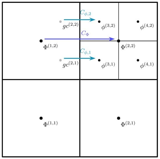
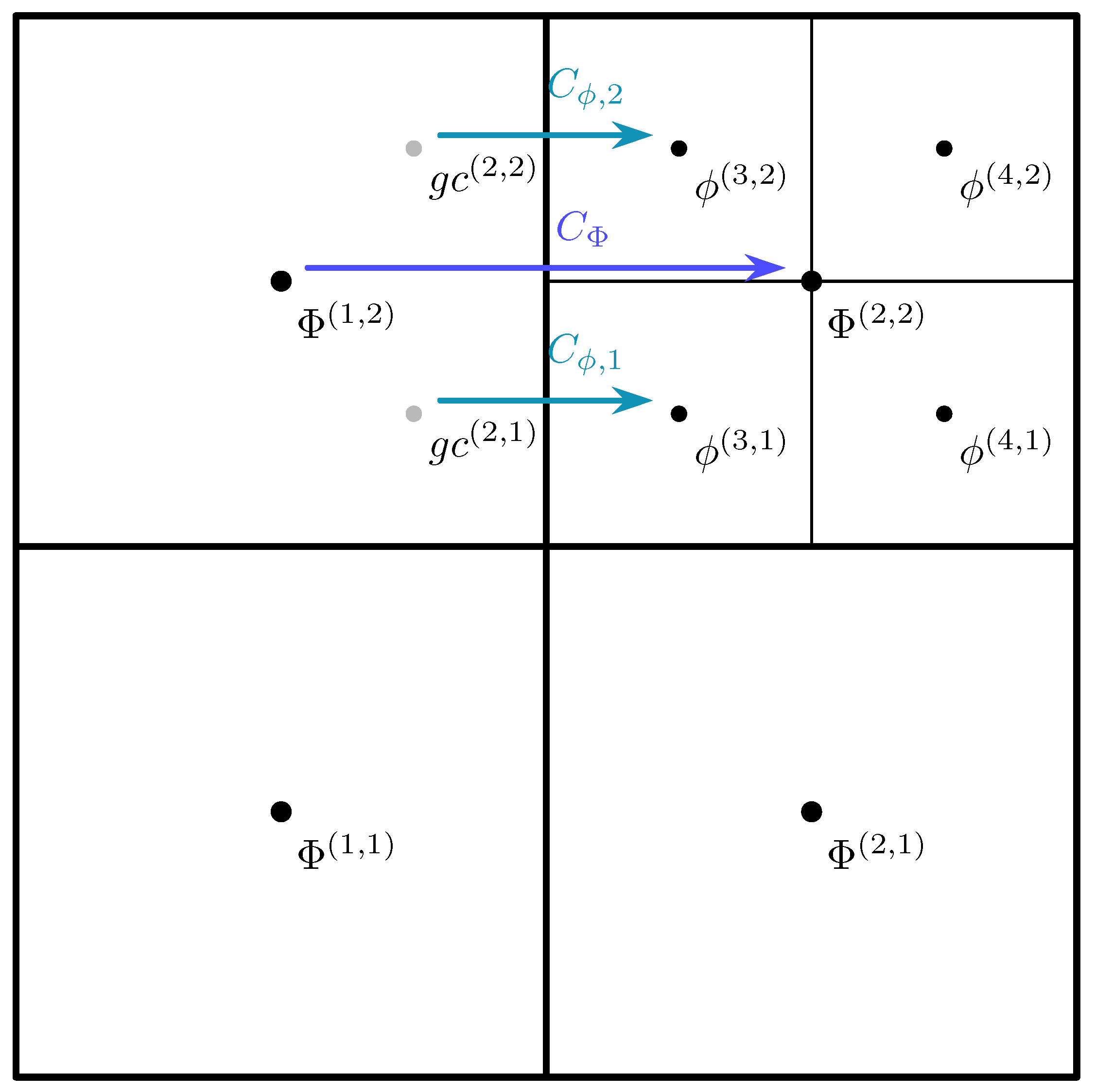
As illustrated in Figure 3, the ghost cells $g{c}^{(2,1)}$ and $g{c}^{(2,2)}$ (gray dots) lie on the fine-grid side of a refinement boundary. For example, the value of $g{c}^{(2,1)}$ is computed from the surrounding coarse- and fine-grid cell-centered values using the following:

$$g{c}^{(2,1)}={\displaystyle \frac{1}{2}}{\Phi }^{(1,2)}+{\displaystyle \frac{1}{3}}{\varphi }^{(3,1)}+{\displaystyle \frac{1}{6}}{\Phi }^{(1,1)}$$

(34)

where $\Phi$ denotes coarse-grid cell values and $\varphi$ denotes fine-grid cell values. This interpolation is applied component-wise to all conserved variables.

Figure 3. Illustration of a refinement boundary. Black dots mark cell centers, gray dots represent ghost-cell centers, and arrows denote fluxes across the boundary.

To maintain strict conservation across refinement boundaries, coarse-grid fluxes at refinement interfaces are not computed directly from coarse-grid states. Instead, the fine-grid fluxes $C_{\varphi ,1}$ and $C_{\varphi ,2}$ are first computed in the usual way. If the interface lies on a refinement boundary, the corresponding coarse-grid flux $C_{\Phi }$ is then corrected to ensure conservation by summing (or averaging) these fine-grid contributions:

$$C_{\Phi }={\displaystyle \frac{1}{2}}\left(C_{\varphi ,1}+C_{\varphi ,2}\right),$$

(35)

where $C_{\varphi ,1}$ and $C_{\varphi ,2}$ are the fine-grid fluxes through the two subfaces aligned with the coarse-grid face. It is important to note that $C_{\varphi ,1}$ and $C_{\varphi ,2}$ themselves are not corrected, since their interfaces are not refinement boundaries. Only the parent coarse flux $C_{\Phi }$ is modified to ensure strict conservation between levels. The same correction procedure is applied consistently to both mass and momentum fluxes, thereby guaranteeing global conservation across refinement boundaries.

2.3.3. Refinement Criteria

Adaptive mesh refinement in our model is driven by a set of refinement criteria that determine where cells should be refined or coarsened. These criteria include the refinement level, selected indicator variables, and corresponding threshold values. The choice of indicator variables depends on the physical features of interest for a given problem.

In this study, refinement is guided primarily by changes in water surface elevation $\eta$. We define a refinement indicator $\tau$ based on the magnitude of the second derivatives of $\eta$ in both spatial directions:

$$\tau =\left|{\displaystyle \frac{{\partial }^2\eta }{\partial x^2}}\right|+\left|{\displaystyle \frac{{\partial }^2\eta }{\partial y^2}}\right|$$

(36)

Each cell is tagged for refinement or coarsening according to the following procedure:

• Refinement: A wet cell is marked for refinement if its indicator value $\tau$ exceeds a prescribed upper threshold ${\tau }_{max}$ and its current refinement level is below the maximum allowable level.
• Coarsening (wet cells): If a parent cell has been subdivided into four child cells, and all four child cells have $\tau <{\tau }_{min}$ while their refinement level is above the minimum allowable level, these child cells are removed, and the parent cell is restored.
• Coarsening (dry cells): In fully dry areas, cells refined beyond the minimum level are coarsened to decrease the number of active cells and enhance computational efficiency.

The thresholds ${\tau }_{max}$ and ${\tau }_{min}$ are problem-dependent and are determined through numerical experimentation. This approach ensures that computational resources are focused in regions with strong free-surface curvature or near moving wet-dry fronts, while minimizing resolution in smooth or inactive areas.

2.3.4. Solution Procedure

The overall solution procedure of the present AMR-based shallow-water model can be summarized as follows:

• Initialization: Place the initial set of coarse boxes over the computational domain. Specify initial conditions for water depth and velocity, and impose physical and refinement boundary conditions.
• Mesh generation: Apply the initial refinement criterion to generate the initial adaptive quadtree mesh.
• Time-step determination: Compute the global time step $\Delta t$ from the Courant–Friedrichs–-Lewy (CFL) condition.
• Flux computation: For each leaf box, reconstruct interface states using the non-negative water depth reconstruction (Section 2.2.2). Evaluate numerical fluxes across cell interfaces using the central-upwind scheme (Section 2.2.3). At refinement interfaces, compute coarse-grid fluxes by summing the corresponding fine-grid fluxes as given in Equation (35) to maintain strict conservation.
• Source term evaluation: Discretize bed slope terms using central differences and treat Manning’s friction term semi-implicitly (Section 2.2.4).
• Update conserved variables: Advance the solution in each leaf box according to the finite volume formulation (Equation (5)).
• Mesh adaptation: Recompute the refinement indicator $\tau$ (Equation (36)) and update the quadtree mesh: refine cells exceeding ${\tau }_{max}$ or near wet–dry fronts, and coarsen cells with $\tau <{\tau }_{min}$ or in dry regions.
• Iteration: Repeat Steps 3–7 until the prescribed final simulation time is reached.

3. Numerical Tests

The accuracy and performance of the proposed numerical model are assessed using four test cases, with results compared against available analytical solutions and experimental measurements. The test suite includes the following: (i) a one-dimensional steady flow over a smooth bed hump; (ii) two laboratory-scale dam-break experiments over variable topography involving wetting and drying fronts; (iii) the historical Malpasset dam-break event. All simulations use a gravitational acceleration of $g=9.81\mathrm{m}/{\mathrm{s}}^2$ and water density $\rho =1000\mathrm{kg}/{\mathrm{m}}^3$.

3.1. Transcritical Flow over a Smooth Bed Hump

This benchmark case, originally proposed by Goutal and Maurel [27], is widely used to evaluate the accuracy of numerical treatments of source terms, especially in scenarios with spatially varying bed topography (see also [20,28,29]). The test setup involves a frictionless rectangular channel of length $25\mathrm{m}$, with the bed elevation specified as follows:

$$z_b=\left\{\begin{array}{cc}-0.05{(x-10)}^2+0.2,\hfill & 8<x<12,\hfill \\ 0,\hfill & \mathrm{otherwise}.\hfill \end{array}\right.$$

(37)

According to Goutal and Maurel [27], different boundary conditions can produce subcritical, supercritical, or transcritical flows, the latter possibly including a hydraulic jump. In this work, the test focuses on the transcritical flow with a hydraulic jump, a particularly challenging scenario for numerical discretizations. The boundary conditions are defined as follows: a constant discharge per unit width of $q=0.18{\mathrm{m}}^2/\mathrm{s}$ at the upstream end, and a fixed water depth of $h=0.33\mathrm{m}$ at the downstream end.

The computational mesh is initialized with 25 coarse boxes, each containing $4\times 4$ uniformly spaced cells. The AMR configuration allows a maximum refinement level of 4, with the refinement and coarsening indicators given in Equation (36), using thresholds ${\tau }_{max}=1.0\times {10}^{-4}$ for refinement and ${\tau }_{min}=2.5\times {10}^{-5}$ for coarsening. The initial condition specifies a free-surface elevation of $\eta =0.33\mathrm{m}$ and a uniform discharge per unit width of $q=0.18{\mathrm{m}}^2/\mathrm{s}$ throughout the domain. The total simulation time is 200 s until steady state is achieved.

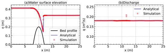
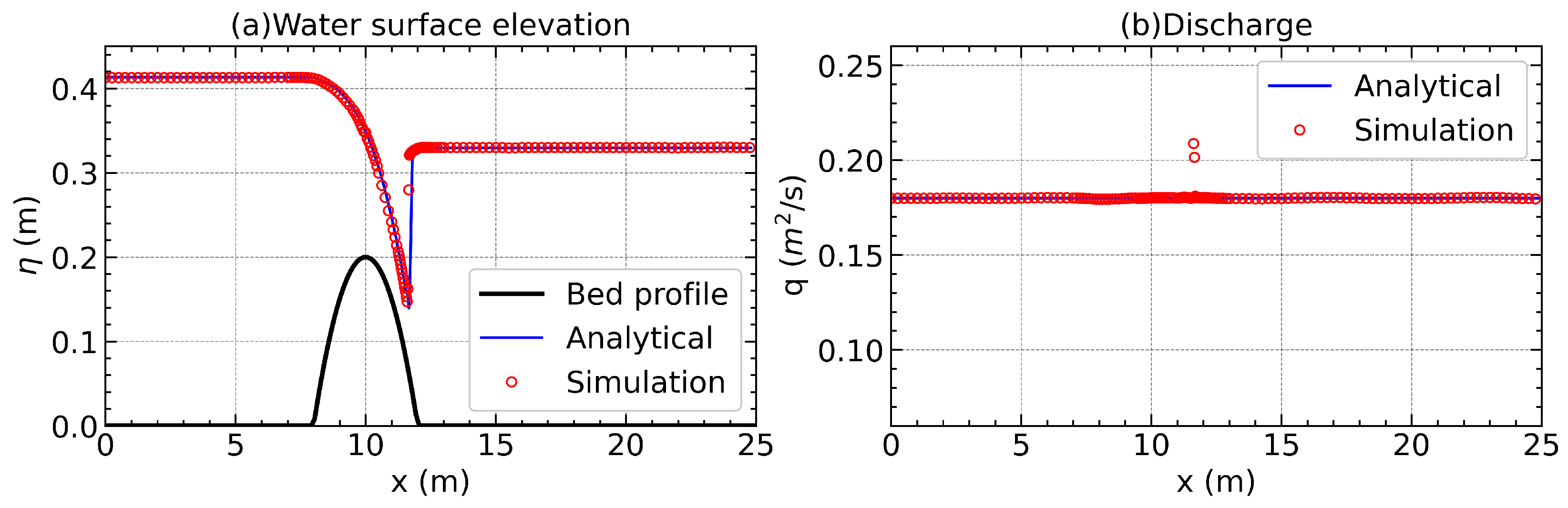
The results of the transcritical hump test with a hydraulic jump are displayed in Figure 4. It can be found that the model correctly resolves the subcritical–supercritical transition over the hump crest and reproduces both the location and profile of the downstream hydraulic jump. For the water surface elevation (Figure 4a), the numerical predictions closely match the analytical profile throughout the domain, demonstrating the model’s ability to simulate steady state without generating spurious oscillations, even in the presence of rapidly varying bed topography. As shown in Figure 4b, the simulated unit discharge closely follows the theoretical value, with a maximum relative error of roughly 15% observed in the vicinity of the hydraulic jump. This level of deviation is consistent with prior findings, including 23% reported by Valiani and Begnudelli [30], 15% by Liang and Borthwick [20], and 10% by Zhou et al. [28].

Figure 4. Steady flow over a hump—transcritical flow with a shock: (a) water surface elevation; (b) discharge.

The AMR grid distribution for this case reveals that refinement is concentrated in regions of steep gradients, particularly around the hump crest and the hydraulic jump, while coarser resolution is maintained elsewhere. This targeted refinement ensures that the complex flow features are well-resolved without excessive grid density in smooth-flow regions.

3.2. Dam-Break Flow over a Triangular Obstacle

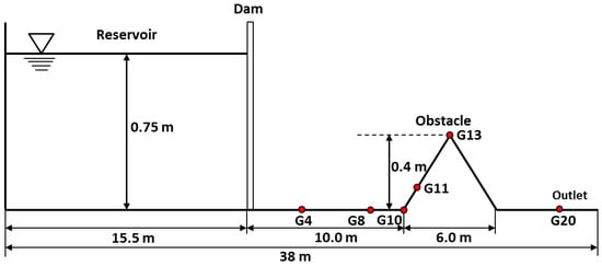
The laboratory experiment of dam-break flow over a triangular obstacle, conducted within the framework of CADAM project [31], is used to evaluate the present model’s capability to simulate dam-break flows with wetting and drying over irregular topography.

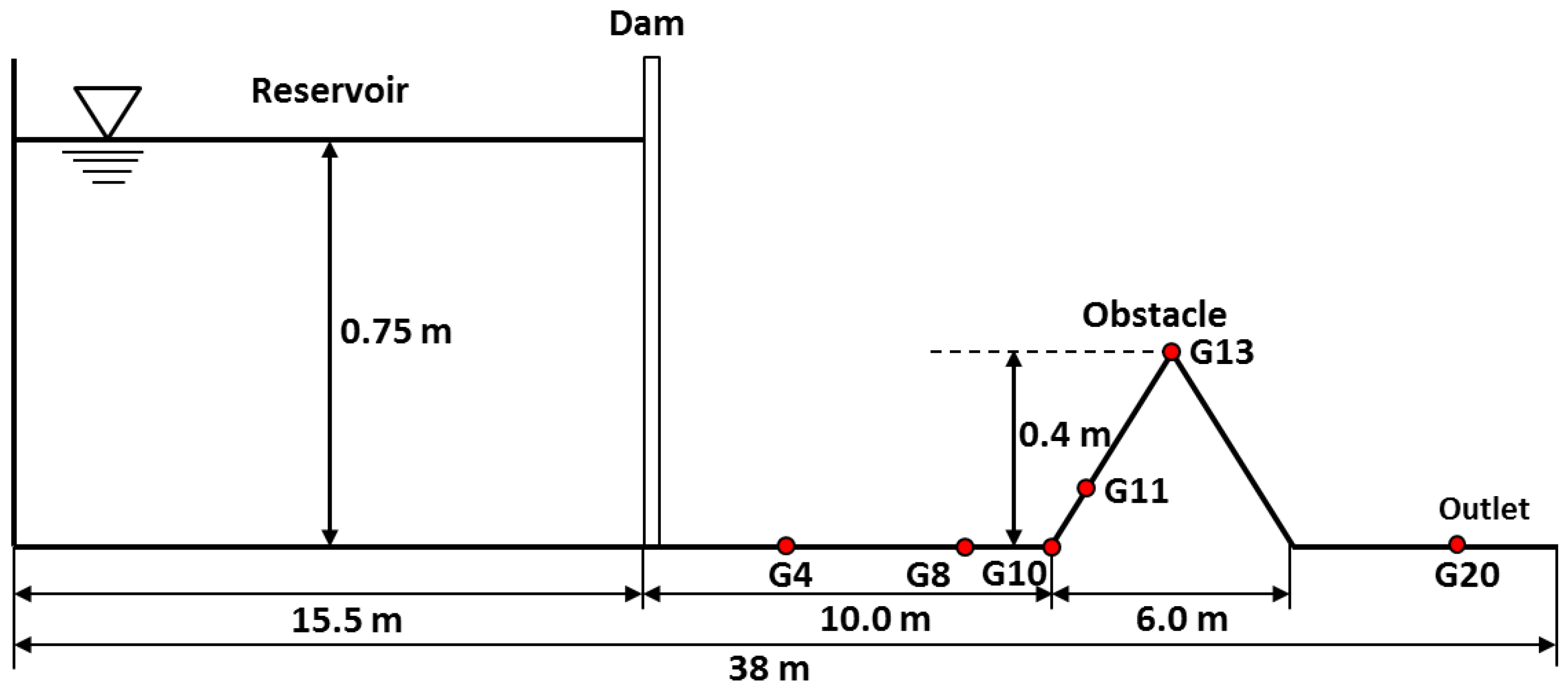
As shown in Figure 5, the experiment is conducted in a straight, rectangular flume of total length $38\mathrm{m}$. A vertical dam is located $15.5\mathrm{m}$ from the upstream end, separating an upstream reservoir from the downstream channel. The initial still-water depth in the reservoir is $0.75\mathrm{m}$; the downstream bed is initially dry. A symmetric triangular obstacle is positioned downstream of the dam. The toe of the obstacle lies $10.0\mathrm{m}$ downstream of the dam, the obstacle length is $6.0\mathrm{m}$, and the crest rises $0.4\mathrm{m}$ above the bed. At $t=0$ s, the dam is instantaneously removed to generate a dam-break wave. Water depth is monitored at six locations (G20, G13, G11, G10, G8, and G4) located in the downstream channel. The upstream boundary is treated as a solid wall, while the downstream boundary is modeled as a free outlet.

Figure 5. Experimental configuration of the CADAM dam-break test with a triangular obstacle.

For the numerical simulation, the computational domain is discretized into $38\times 4$ coarse boxes, each containing $4\times 4$ uniformly spaced cells. The maximum refinement level is set to $l_{\max }=4$, with refinement and coarsening thresholds of ${\tau }_{\max }=1.0\times {10}^{-4}$ and ${\tau }_{\min }=2.5\times {10}^{-5}$, respectively. Consistent with Liang and Marche [32], the Manning coefficient is specified as $n=0.0125$. Mesh refinement is concentrated in the vicinity of the obstacle to capture localized flow features, while coarser resolution is maintained elsewhere to reduce computational cost. The simulation time is 90 s.

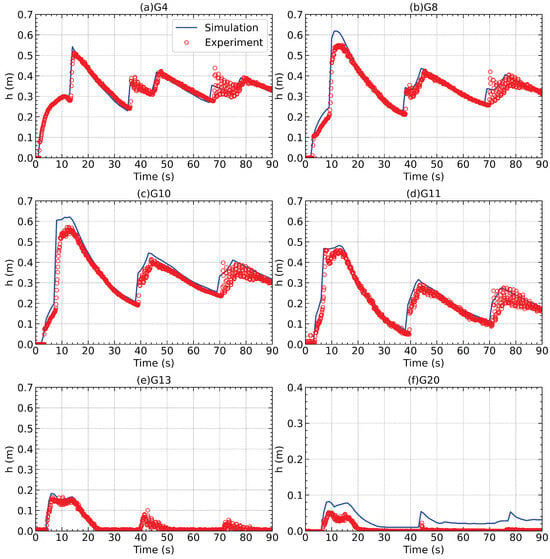
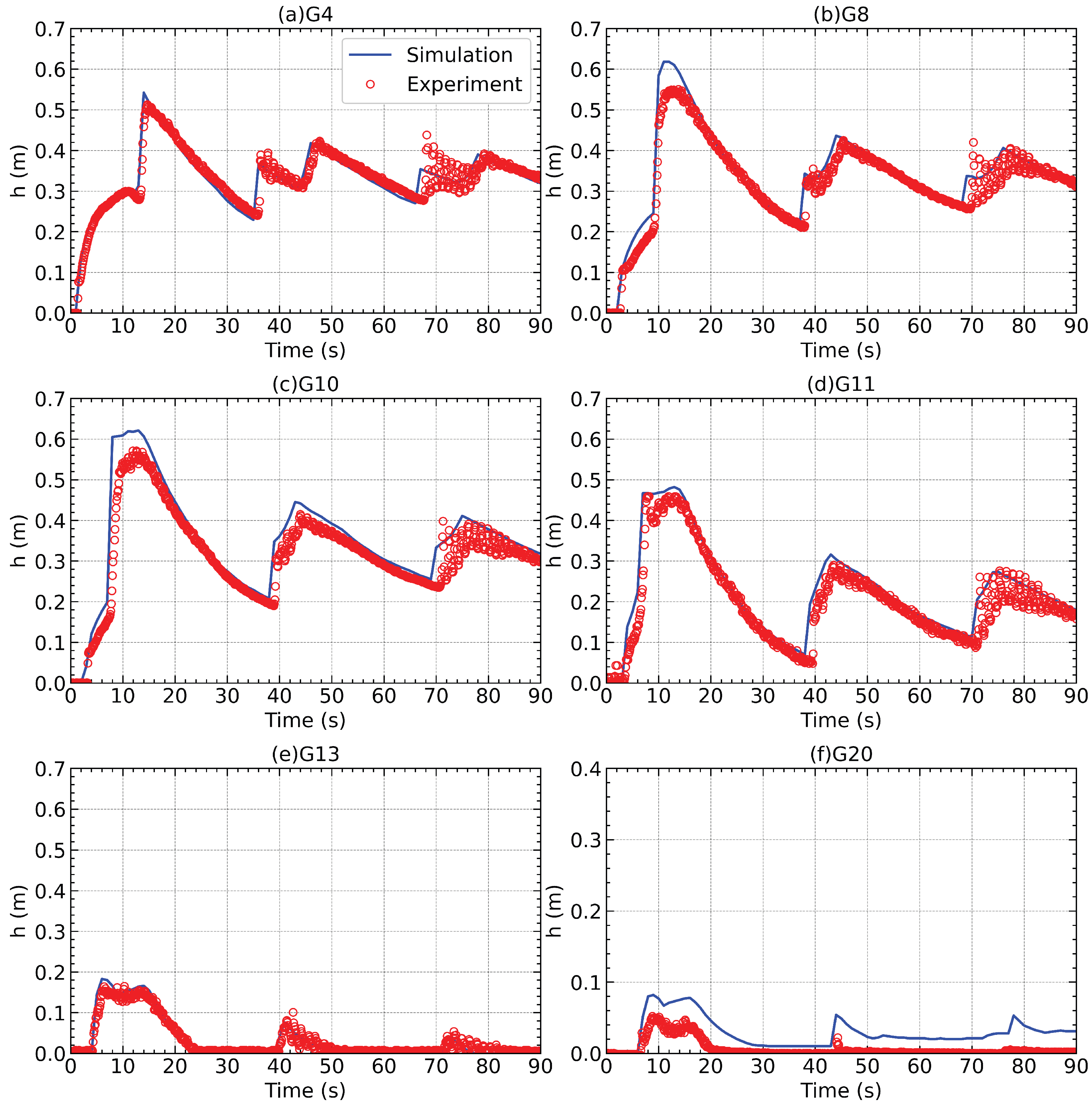
Figure 6 shows a comparison between simulated and measured hydrographs at the six gauges. The model accurately captures both the arrival time and peak magnitude of the leading bore at most sites, and shows good agreement with the observed attenuation and oscillatory behavior thereafter. The most noticeable discrepancy occurs at G20, where the computed water depth is overestimated relative to the measurements. Similar discrepancies at this gauge have been noted in earlier studies with alternative numerical schemes [32,33,34], suggesting that two-dimensional shallow water models may not fully resolve the complex three-dimensional flow structures between the obstacle and the downstream outlet.

Figure 6. Comparison of computed and measured water depth hydrographs at six gauges: (a) G4; (b) G8; (c) G10; (d) G11; (e) G13; (f) G20.

To quantitatively assess the model’s performance, the average discrepancy ($L_1$ norm) between calculated and measured water depths is computed as follows:

$$L_1={\displaystyle \frac{1}{N}}\sum _{n=1}^N\left|{\lambda }_n^{\mathrm{mea}}-{\lambda }_n^{\mathrm{cal}}\right|,$$

where ${\lambda }_n^{\mathrm{mea}}$ and ${\lambda }_n^{\mathrm{cal}}$ represent the measured and calculated water depths, respectively, and N indicates the total number of records at a given gauge. The calculated $L_1$ values are 0.023 m at G20, 0.009 m at G13, 0.031 m at G11, 0.030 m at G10, 0.019 m at G8 and 0.017 m at G4. The results confirm that the proposed AMR framework provides accurate predictions of dam-break wave evolution, effectively handles wet/dry front movement, and resolves complex flow–obstacle interactions over irregular beds.

3.3. Laboratory Experiment of a Partial Dam-Break

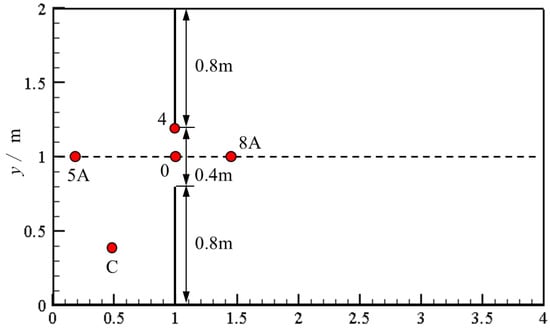
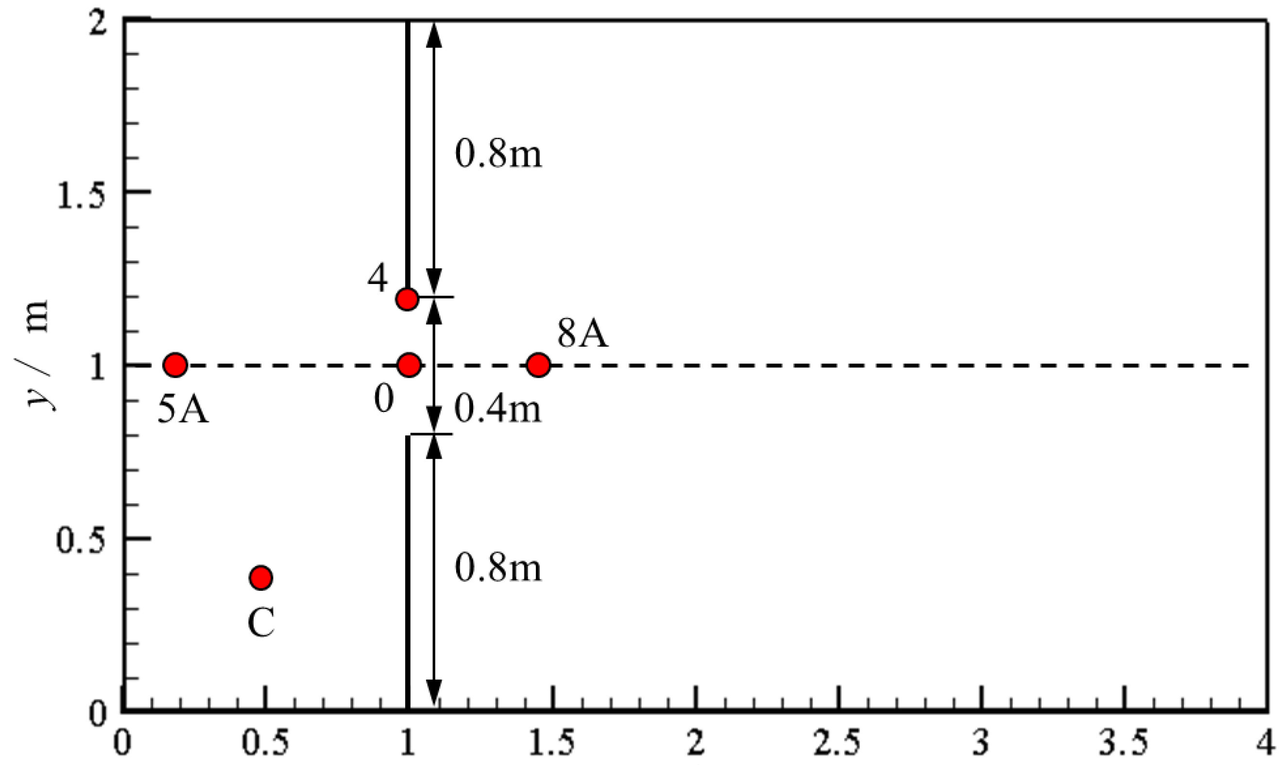
The experiment of Fraccarollo and Toro [35] is used to further assess the model for fully two-dimensional dam-break flows. As shown in Figure 7, the domain is a horizontal rectangle of length $4.0\mathrm{m}$ and width $2.0\mathrm{m}$ ($0\le x\le 4$, $0\le y\le 2$). A vertical dam is located at $x=1.0\mathrm{m}$ and contains a central breach of width $0.4\mathrm{m}$, centered on the midline (i.e., $0.8\le y\le 1.2\mathrm{m}$). The upstream reservoir is initially at rest with a free-surface elevation of $0.6\mathrm{m}$, while the downstream floodplain $(x>1)$ is dry.

Figure 7. Setup of the partial dam-break experiment.

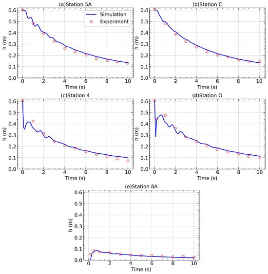
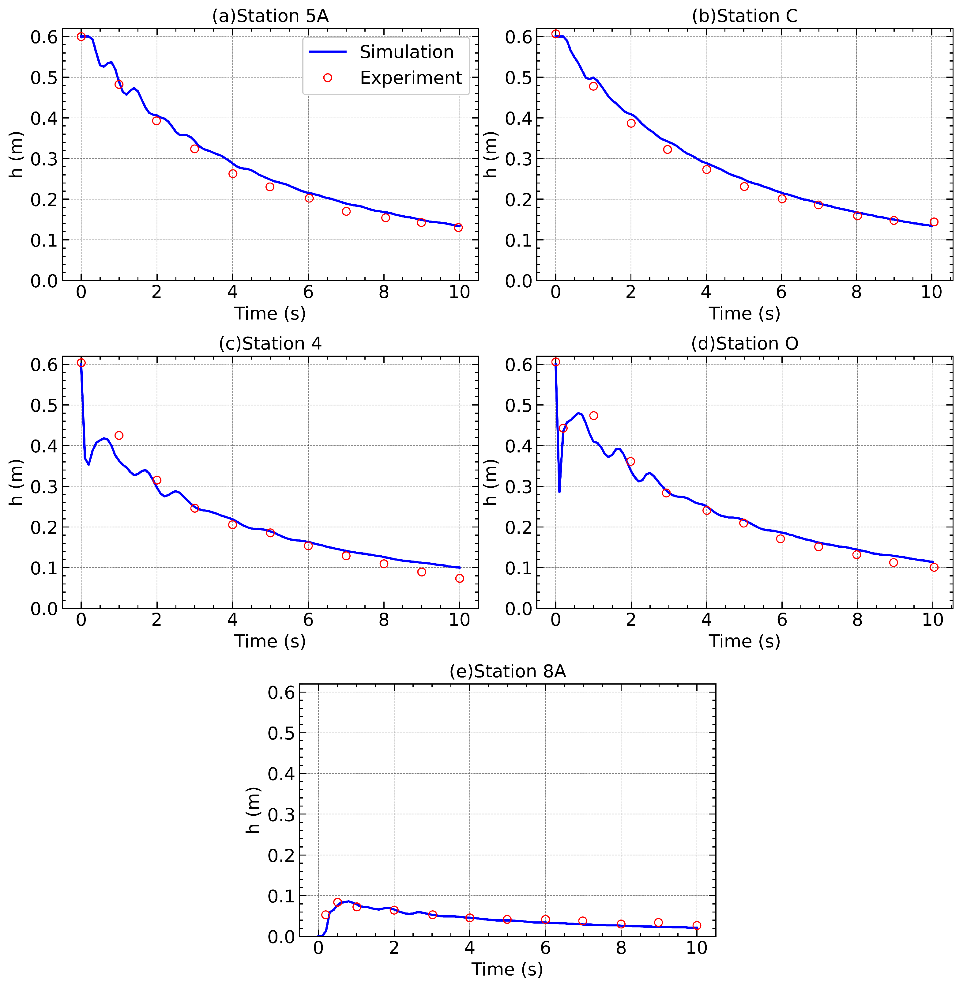
At $t=0\mathrm{s}$, the breached segment is instantaneously opened, releasing water onto the floodplain. Solid-wall conditions are imposed at the upstream boundary $(x=0)$, and transmissive conditions are applied at $x=4$ and along the lateral boundaries $y=0$ and $y=2$. Water depth is recorded at five gauge locations (Table 1) to provide a time series for validation.

Table 1. Locations of gauge stations in the experimental setup.

Gauges	5A	C	4	0	8A
x-coordinate (m)	0.180	0.480	1.000	1.000	1.720
y-coordinate (m)	1.000	0.400	1.160	1.000	1.000

For the numerical simulation, the domain is partitioned into $20\times 10$ coarse boxes, each containing $2\times 2$ uniformly spaced cells, yielding a base resolution of $\Delta x=\Delta y=0.10\mathrm{m}$. The maximum refinement level is set to $l_{\max }=4$. Cells are refined or coarsened according to the indicator in Equation (36), using thresholds ${\tau }_{\max }=1.0\times {10}^{-5}$ and ${\tau }_{\min }=2.5\times {10}^{-6}$. Refinement is concentrated near the breach and along moving wet–dry fronts, while smooth-flow regions remain coarse to reduce computational cost.

The simulation is run to $t=10\mathrm{s}$. Figure 8 compares the simulated and measured water-depth time series at the five gauges. The model accurately reproduces both the arrival times and magnitudes of the leading wave, as well as the subsequent oscillations in water depth. The close agreement with experimental data demonstrates the ability of the present AMR-based model to handle two-dimensional dam break flow with wetting and drying processes.

Figure 8. Comparison of simulated and observed water depth hydrographs at five gauges in the partial dam-break test.

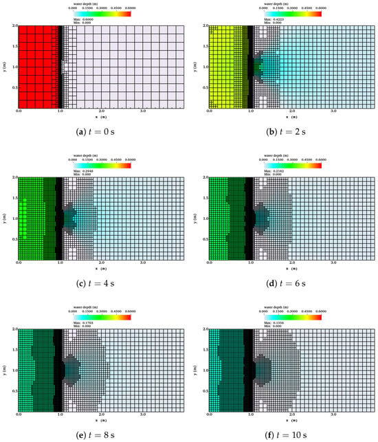
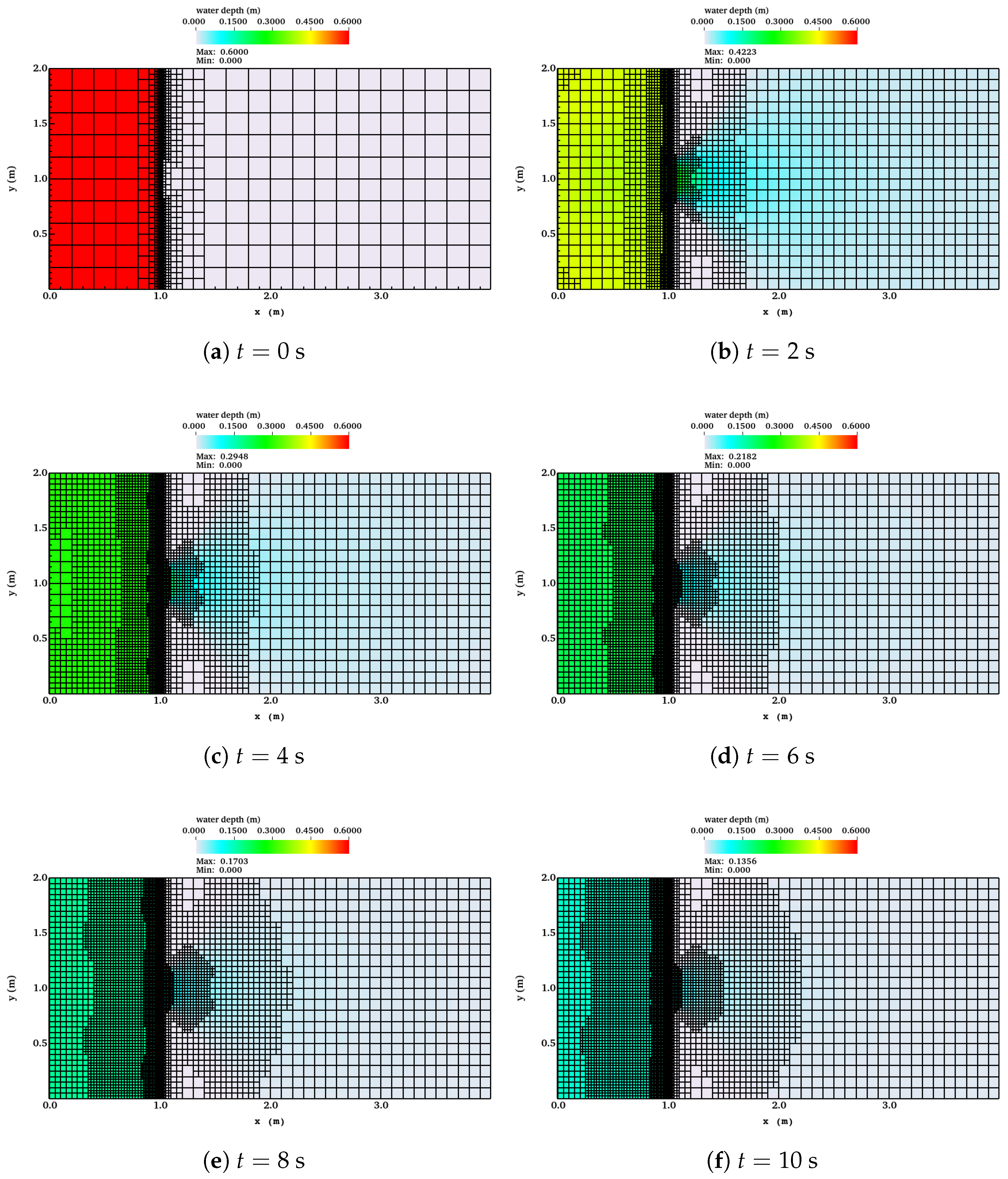
Figure 9 presents snapshots of water depth contours together with the adapted quadtree mesh at $t=0$, 2, 4, 6, 8, and 10 s. The results show that mesh refinement dynamically follows the rapidly evolving wet/dry interface and high-gradient regions near the breach, while coarse resolution is maintained in quiescent areas, achieving a balance between accuracy and computational efficiency.

Figure 9. Snapshots of water depth contours and adapted quadtree mesh for the partial dam-break experiment.

3.4. Historical Dam-Break Flood Simulation

The Malpasset Dam, situated about 12 km upstream of Fréjus, France, was a thin-arch concrete structure designed to retain a reservoir of $5\times {10}^6{\mathrm{m}}^3$. At 21:14 local time on 2 December 1959, the Malpasset Dam failed, releasing a destructive flood wave that propagated along the Reyran River valley to the Mediterranean. The disaster resulted in 433 fatalities and extensive destruction of infrastructure [36]. The event is widely recognized as a challenging real-world benchmark for shallow-water solvers due to the highly energetic flow through a narrow gorge followed by rapid expansion over a broad alluvial fan.

3.4.1. Computational Setup

The digital elevation model (DEM) originates from the CADAM project [37] and consists of 13,541 irregularly spaced surveyed points, interpolated onto overlapping Cartesian grids with 2, 5, and 20 m resolutions [38]. The computational domain spans 16.2 km × 6.2 km and is initially discretized into $31\times 81$ coarse boxes, each containing $2\times 2$ cells, giving a base grid spacing of $\Delta x=\Delta y=100$ m. A maximum refinement level of $l_{\max }=3$ is imposed, corresponding to a finest resolution of 25 m. Refinement is based solely on wetness: Wet cells are refined to the highest resolution level. The Manning coefficient is specified as $0.033$ [38]. Boundary conditions consist of a sea level of 0 m at the downstream outlet and solid walls elsewhere. The reservoir is initialized with a water surface elevation of 100 m above sea level, and instantaneous breach failure is assumed at $t=0$ s.

3.4.2. Simulation Overview

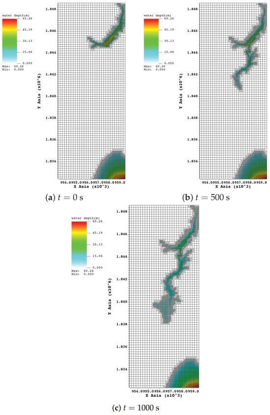
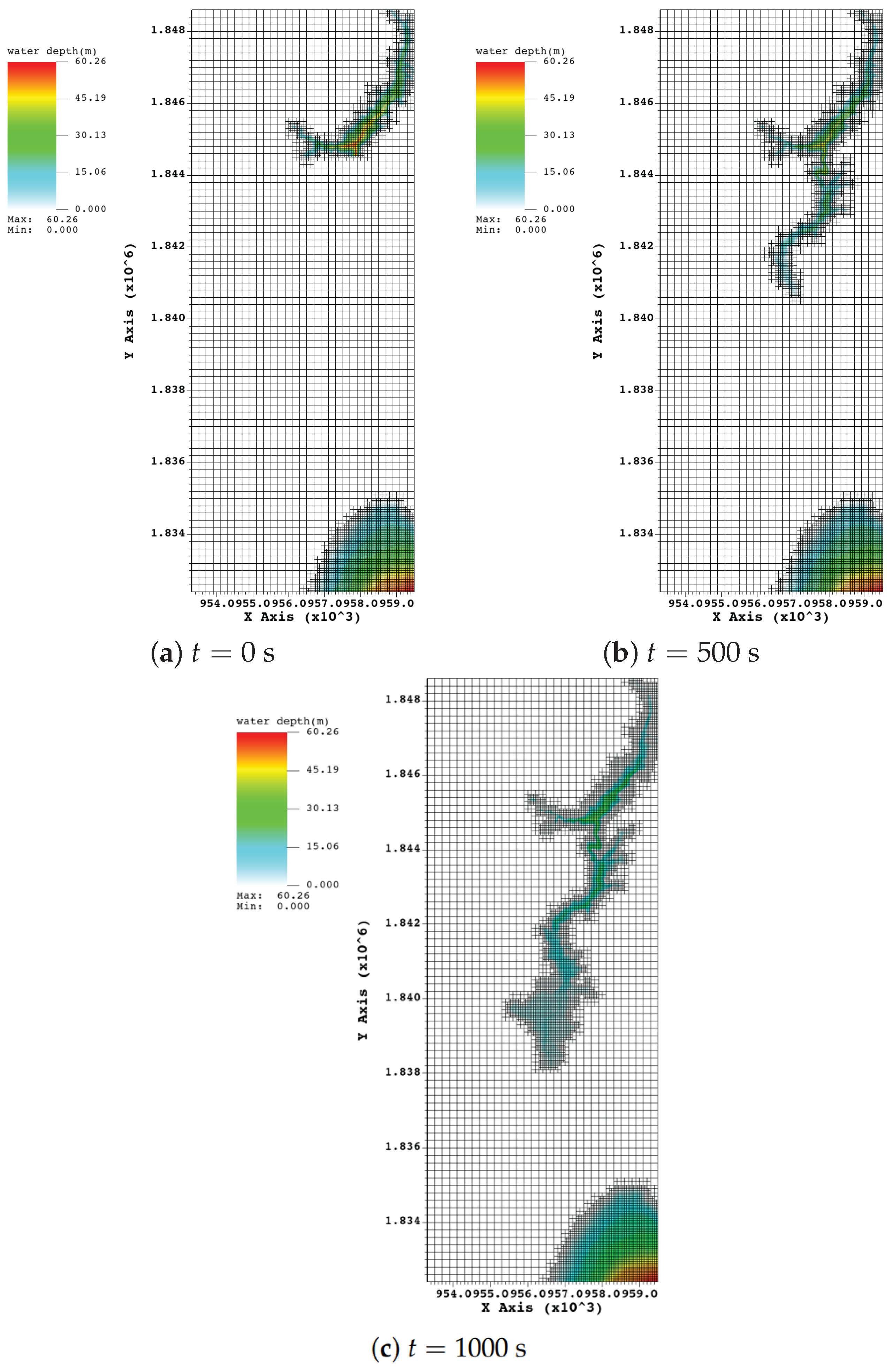
Snapshots of simulated water depth and the adaptive quadtree mesh at $t=0$ s, 500 s, and 1000 s are shown in Figure 10. The AMR algorithm dynamically concentrates resolution along the advancing flood front, particularly in the gorge and over the urban floodplain, while unaffected areas remain at the coarsest level, thereby optimizing computational efficiency.

Figure 10. Snapshots of water depth contours and adaptive quadtree mesh for the Malpasset dam-break simulation at selected times.

3.4.3. Validation Against Field and Laboratory Data

Model validation is conducted against two independent datasets:

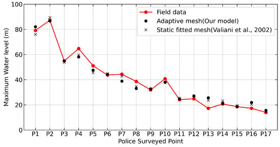
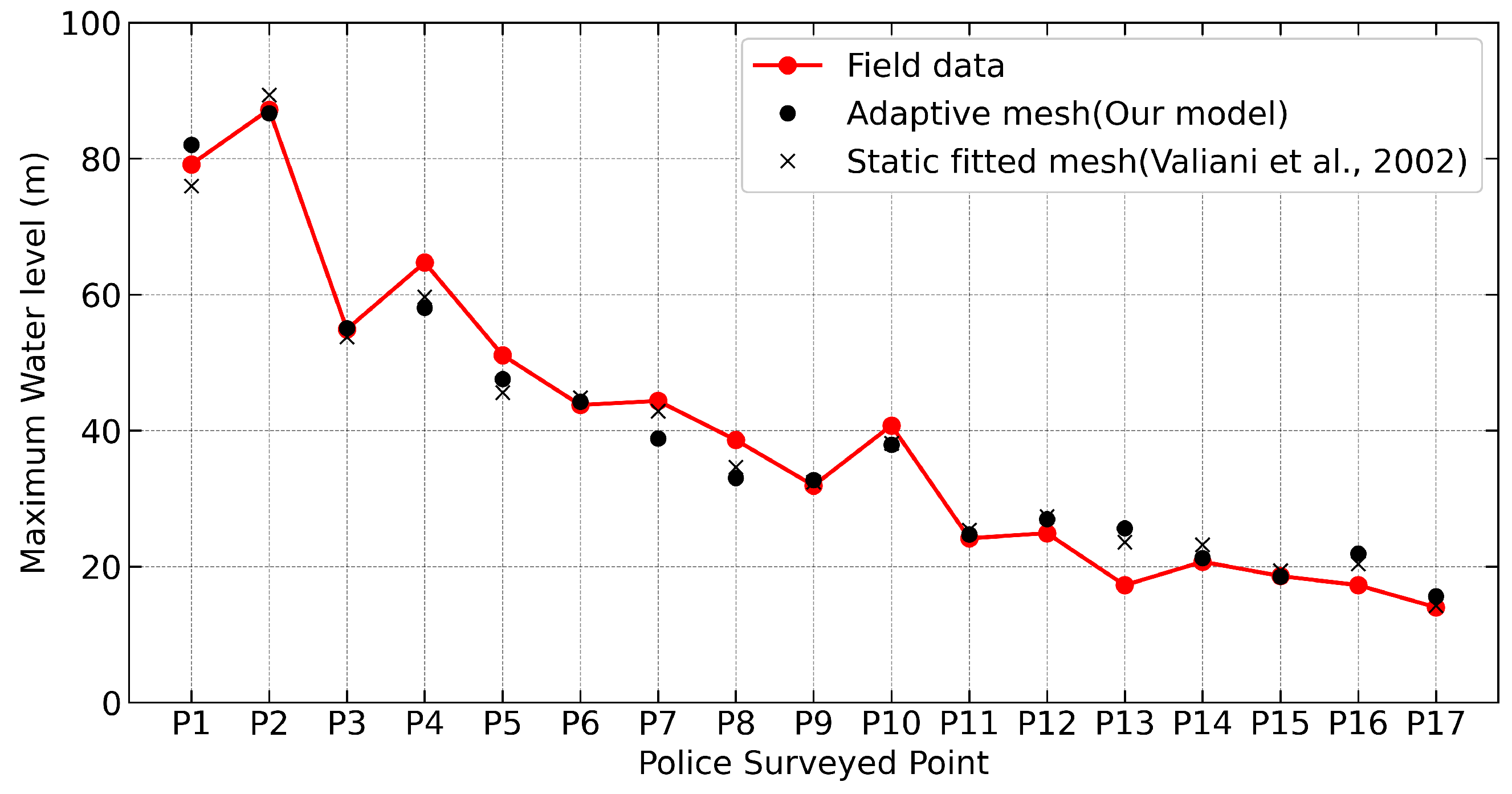
• Maximum water levels from 17 field-surveyed high-water marks (“police-surveyed points”) downstream of the dam after the 1959 event.
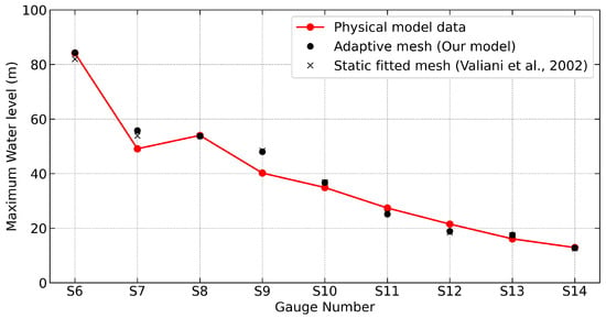
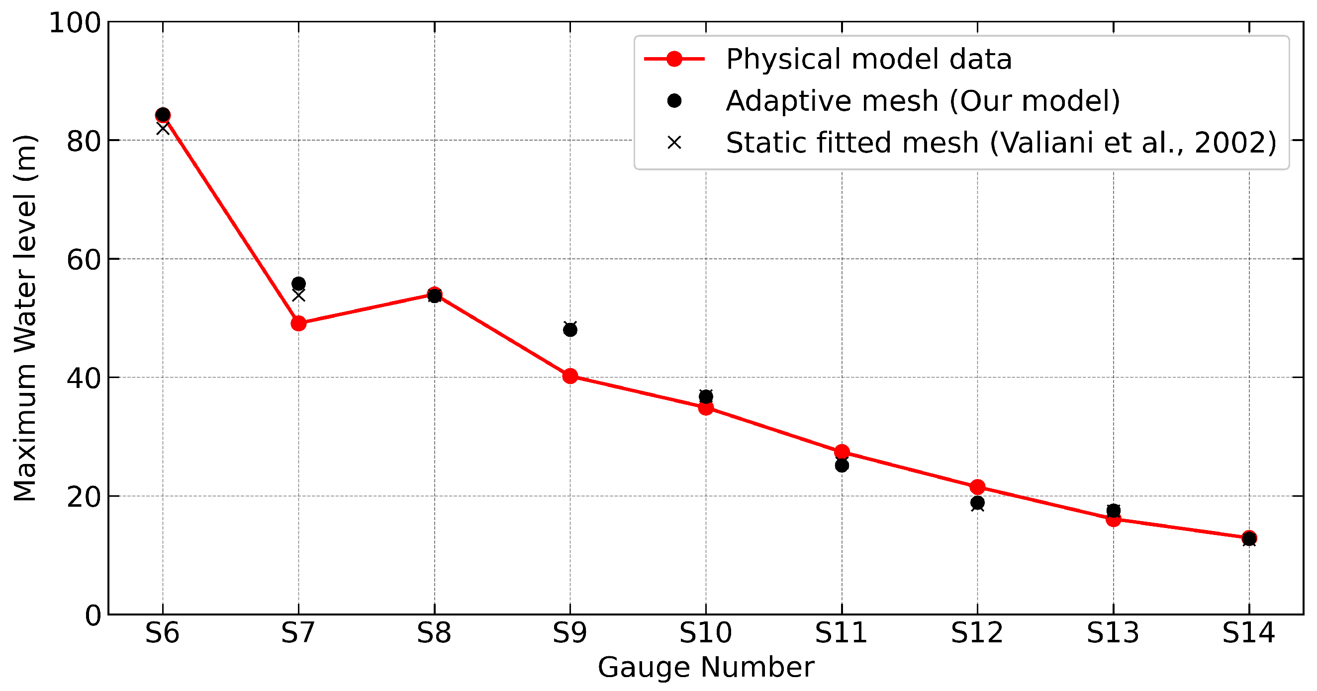
• Maximum water levels from 9 gauge locations in a 1:400 laboratory model [37].

The police-surveyed points (P1–P17) are located near the inundation margins, where flows were shallow and strongly influenced by wet–dry interface resolution. In contrast, the scale-model gauges (S6–S14) were positioned in the main body of the flood wave.

Figure 11 and Figure 12 compare the present AMR model results with measurements and simulation results of Valiani et al. [36], which used an unstructured mesh fitted to the topography. For the field-surveyed points, the present model captures both the overall trend and local variability, with deviations within the range reported in previous studies. For the laboratory-scale gauges, agreement is generally closer, consistent with earlier findings [38] that measurements within the main flow are less affected by wet–dry boundary uncertainties. These results confirm that the present AMR-based solver attains predictive accuracy comparable to established numerical approaches.

Figure 11. Comparison of maximum water levels at 17 field-surveyed high-water mark locations (P1–P17) between the present AMR model, field measurements, and Valiani’s simulation [36].

Figure 12. Comparison of maximum water levels at 9 laboratory-scale model gauges (S6–S14) between the present AMR model, laboratory measurements, and Valiani’s simulation [36].

3.4.4. Computational Performance

Computational efficiency is assessed by comparing the AMR simulation with a fixed fine-mesh simulation of uniform 25 m resolution. Both simulations were executed on a laptop with an Intel Core i7 processor (2.3 GHz) and 32 GB of RAM, covering 2000 s of physical time. The AMR simulation required approximately 1440 s of wall-clock time, while the fixed fine-mesh run took about 2340 s. The AMR approach achieved a similar level of accuracy while reducing the total number of active cells by over an order of magnitude, leading to substantial savings in both computational time and memory usage.

4. Conclusions

A 2D depth-averaged shallow water model has been developed on a block-structured quadtree adaptive mesh within the open-source Afivo framework. The model couples a positivity-preserving, well-balanced central-upwind scheme with non-negative water depth reconstruction, achieving second-order spatial accuracy and robustly handling wetting and drying processes. Mass conservation across refinement levels is ensured by computing coarse-grid fluxes from the sum of fine-grid fluxes, while mesh adaptation driven by gradients in water surface elevation focuses resolution in dynamically active regions, enhancing computational efficiency without compromising accuracy.

Validation of the model was carried out against three standard benchmarks and a field-scale dam-break event: steady transcritical flow over a hump, two laboratory dam-break experiments involving wet/dry fronts and obstacles, and the historical Malpasset dam-break flood. The close agreement of the numerical results with analytical solutions and experimental data confirms the model’s ability to reproduce steady flows, track wet/dry fronts, and simulate large-scale flood events over steep and complex terrain. Moreover, compared with a uniformly fine mesh, the AMR strategy significantly reduces the number of active cells, resulting in substantial savings in CPU time and memory, making it a practical and efficient tool for high-resolution flood simulation and hazard assessment over complex natural topography.

References

- Shaw, J.; Kesserwani, G.; Neal, J.; Bates, P.; Sharifian, M.K. LISFLOOD-FP 8.0: The new discontinuous Galerkin shallow-water solver for multi-core CPUs and GPUs. Geosci. Model Dev. 2021, 14, 3577–3602. [Google Scholar] [CrossRef] [Scilit]
- Ferrari, A.; Vacondio, R.; Mignosa, P. High-resolution 2D shallow water modelling of dam failure floods for emergency action plans. J. Hydrol. 2023, 618, 129192. [Google Scholar] [CrossRef] [Scilit]
- Bonev, B.; Hesthaven, J.S.; Giraldo, F.X.; Kopera, M.A. Discontinuous Galerkin scheme for the spherical shallow water equations with applications to tsunami modeling and prediction. J. Comput. Phys. 2018, 362, 425–448. [Google Scholar] [CrossRef] [Scilit]
- D’Alpaos, L.; Defina, A. Mathematical modeling of tidal hydrodynamics in shallow lagoons: A review of open issues and applications to the Venice lagoon. Comput. Geosci. 2007, 33, 476–496. [Google Scholar] [CrossRef] [Scilit]
- Roe, P.L. Approximate Riemann solvers, parameter vectors, and difference schemes. J. Comput. Phys. 1981, 43, 357–372. [Google Scholar] [CrossRef] [Scilit]
- Harten, A. High resolution schemes for hyperbolic conservation laws. J. Comput. Phys. 1997, 135, 260–278. [Google Scholar] [CrossRef] [Scilit]
- Toro, E.F.; Spruce, M.; Speares, W. Restoration of the contact surface in the HLL-Riemann solver. Shock Waves 1994, 4, 25–34. [Google Scholar] [CrossRef] [Scilit]
- Friedrichs, K.O. Symmetric hyperbolic linear differential equations. Commun. Pure Appl. Math. 1954, 7, 345–392. [Google Scholar] [CrossRef] [Scilit]
- Lax, P.D. Weak solutions of nonlinear hyperbolic equations and their numerical computation. In Selected Papers Volume I; Springer: Berlin/Heidelberg, Germany, 2005; pp. 198–232. [Google Scholar]
- Kurganov, A.; Petrova, G. A second-order well-balanced positivity preserving central-upwind scheme for the Saint-Venant system. Commun. Math. Sci. 2007, 5, 133–160. [Google Scholar] [CrossRef] [Scilit]
- Wu, G.; He, Z.; Zhao, L.; Liu, G. A well-balanced positivity preserving two-dimensional shallow flow model with wetting and drying fronts over irregular topography. J. Hydrodyn. 2018, 30, 618–631. [Google Scholar] [CrossRef] [Scilit]
- Ginting, B.M.; Mundani, R.P. Comparison of Shallow Water Solvers: Applications for Dam-Break and Tsunami Cases with Reordering Strategy for Efficient Vectorization on Modern Hardware. Water 2019, 11, 639. [Google Scholar] [CrossRef] [Scilit]
- Zhou, Z.Q.; Mi, J.Y. Numerical modeling of shallow-water flows on Cartesian grids. J. Hydraul. Eng. 2001, 127, 191–198. [Google Scholar]
- Bates, P.D.; Horritt, M.S.; Fewtrell, T.J. A simple inertial formulation of the shallow water equations for efficient two-dimensional flood inundation modelling. J. Hydrol. 2010, 387, 33–45. [Google Scholar] [CrossRef] [Scilit]
- Liu, Y.; Li, X.; Chen, L. A well-balanced positivity-preserving finite-volume scheme for shallow water equations on Cartesian grids. Adv. Water Resour. 2019, 129, 48–61. [Google Scholar] [CrossRef] [Scilit]
- Carlotto, T.; Chaffe, P.L.B.; dos Santos, C.I.; Lee, S. SW2D-GPU: A two-dimensional shallow water model accelerated by GPGPU. Environ. Model. Softw. 2021, 145, 105205. [Google Scholar] [CrossRef] [Scilit]
- Berger, M.J.; George, D.L.; LeVeque, R.J.; Mandli, K.T. The GeoClaw software for depth-averaged flows with adaptive refinement. Adv. Water Resour. 2011, 34, 1195–1206. [Google Scholar] [CrossRef] [Scilit]
- Liang, Q.; Borthwick, A.G.L. Adaptive quadtree simulation of shallow flows with wetting and drying over complex topography. Comput. Fluids 2007, 36, 1457–1471. [Google Scholar] [CrossRef] [Scilit]
- Liang, Q.; Du, G.; Hall, J.W.; Borthwick, A.G.L. Flood Inundation Modeling with an Adaptive Quadtree Grid Shallow Water Equation Solver. J. Hydraul. Eng. 2008, 134, 1603–1610. [Google Scholar] [CrossRef] [Scilit]
- Liang, Q.; Borthwick, A.G.L. Adaptive quadtree simulation of shallow flows with wet–dry fronts over complex topography. J. Comput. Phys. 2009, 228, 3240–3258. [Google Scholar] [CrossRef] [Scilit]
- Kirstetter, G.; Delestre, O.; Lagrée, P.Y.; Popinet, S.; Josserand, C. B-flood 1.0: An open-source Saint-Venant model for flash-flood simulation using adaptive refinement. Geosci. Model Dev. 2021, 14, 7117–7132. [Google Scholar] [CrossRef] [Scilit]
- Kyanjo, B.; Calhoun, D.; George, D.L. GeoFlood (v1. 0.0): Computational model for overland flooding. EGUsphere 2025, 2025, 1. [Google Scholar]
- Calhoun, D.; Burstedde, C. ForestClaw: A parallel algorithm for patch-based adaptive mesh refinement on a forest of quadtrees. arXiv 2017, arXiv:1703.03116. [Google Scholar]
- Deschrijver, T.; Teunissen, J.; Ebert, U. Afivo: A framework for quadtree/octree AMR with shared-memory parallelization and geometric multigrid methods. Comput. Phys. Commun. 2019, 233, 39–49. [Google Scholar] [CrossRef] [Scilit]
- Liang, Q. Flood simulation using a well-balanced shallow flow model. J. Hydraul. Eng. 2010, 136, 669–675. [Google Scholar] [CrossRef] [Scilit]
- Audusse, E.; Bouchut, F.; Bristeau, M.O.; Klein, R.; Perthame, B.T. A fast and stable well-balanced scheme with hydrostatic reconstruction for shallow water flows. SIAM J. Sci. Comput. 2004, 25, 2050–2065. [Google Scholar] [CrossRef] [Scilit]
- Goutal, N.; Maurel, F. Proceedings of the 2nd Workshop on Dam-Break Wave Simulation; Départment Laboratoire National d’Hydraulique, Groupe Hydraulique Fluviale Electricité de France: Toulouse, France, 1997. [Google Scholar]
- Zhou, J.G.; Causon, D.M.; Mingham, C.G.; Ingram, D.M. The surface gradient method for the treatment of source terms in the shallow-water equations. J. Comput. Phys. 2001, 168, 1–25. [Google Scholar] [CrossRef] [Scilit]
- Delis, A.I.; Skeels, C.P.; Sotiropoulos, F. A robust high-resolution finite volume scheme for the simulation of free surface shallow flows. J. Hydraul. Res. 2000, 38, 197–204. [Google Scholar] [CrossRef] [Scilit]
- Valiani, A.; Begnudelli, L. Divergence form for bed slope source term in shallow water equations. J. Hydraul. Eng. 2006, 132, 652–665. [Google Scholar] [CrossRef] [Scilit]
- Morris, M. CADAM: Concerted action on dam-break modeling–Final report. Rep. No. SR 2000, 571, 1–33. [Google Scholar]
- Liang, Q.; Marche, F. Numerical resolution of well-balanced shallow water equations with complex source terms. Adv. Water Resour. 2009, 32, 873–884. [Google Scholar] [CrossRef] [Scilit]
- Brufau, P.; Garcia-Navarro, P. Two-dimensional dam break flow simulation. Int. J. Numer. Methods Fluids 2000, 33, 35–57. [Google Scholar] [CrossRef] [Scilit]
- Liang, D.; Falconer, R.A.; Lin, B. Comparison between TVD-MacCormack and ADI-type solvers of the shallow water equations. Adv. Water Resour. 2006, 29, 1833–1845. [Google Scholar] [CrossRef] [Scilit]
- Fraccarollo, L.; Toro, E.F. Experimental and numerical assessment of the shallow water model for two-dimensional dam-break type problems. J. Hydraul. Res. 1995, 33, 843–864. [Google Scholar] [CrossRef] [Scilit]
- Valiani, A.; Caleffi, V.; Zanni, A. Case study: Malpasset dam-break simulation using a two-dimensional finite volume method. J. Hydraul. Eng. 2002, 128, 460–472. [Google Scholar] [CrossRef] [Scilit]
- Soares Frazao, S.; Alcrudo, F.; Goutal, N. Dam-break test cases summary. In Proceedings of the 4th CADAM Meeting: Concerted Action on Dam-Break Modelling, Zaragoza, Spain, 18–19 November 1999. [Google Scholar]
- George, D. Adaptive finite volume methods with well-balanced Riemann solvers for modeling floods in rugged terrain: Application to the Malpasset dam-break flood (France, 1959). Int. J. Numer. Methods Fluids 2011, 66, 1000–1018. [Google Scholar] [CrossRef] [Scilit]
Disclaimer/Publisher’s Note: The statements, opinions and data contained in all publications are solely those of the individual author(s) and contributor(s) and not of MDPI and/or the editor(s). MDPI and/or the editor(s) disclaim responsibility for any injury to people or property resulting from any ideas, methods, instructions or products referred to in the content. |
© 2025 by the authors. Licensee MDPI, Basel, Switzerland. This article is an open access article distributed under the terms and conditions of the Creative Commons Attribution (CC BY) license (https://creativecommons.org/licenses/by/4.0/).