Pesticides and Their Metabolites in Amphibian Spawning Waters Are Positively Associated with Nearby Arable Land

Abstract

Pesticides pose risks to human health and the environment. Monitoring schemes often exclude small sites with fluctuating water levels, inhabited by many species, including amphibians. We sampled for pesticides and their metabolites in 68 amphibian spawning waters in Austria. We analyzed the number of pesticides and concentrations in relation to the surrounding land use. We tested for 165 pesticides and metabolites and found 54; 46% were herbicides. The median total pesticide concentration per site was 0.097 µg/L (range: 0–20.419 µg/L). Pesticides found were generally of lower toxicity. We calculated the pesticide toxicity for aquatic invertebrates, fish, birds, and mammals, as proxies for amphibians and the overall ecosystems. Arable land was associated with pesticide number, concentration and toxicity according to the Boruta model selection. However, due to highly variable concentrations (and therefore also variable toxicity) only pesticide number showed significances in a generalized linear model. In this model arable land was positively associated with the number of pesticides detected, while the proportion of grassland, scrubs, artificial surfaces and tree cover had negative effects according to the linear model. Our results highlight (i) a widespread contamination of small temporary water bodies, (ii) the presence of multiple pesticide residues (cocktails), commonly more harmful than single pesticides, at amphibian spawning waters. These results provide a basis for future studies investigating the effects of common pesticide combinations in controlled settings using realistic scenarios and enable better assessment of the potential risks to wildlife.

1. Introduction

Conventional agriculture relies on the heavy use of pesticides and other environmental pollutants, which have often been detected outside their intended areas of effect [1,2,3,4]. Contamination of the surroundings of agricultural areas can occur through drift or runoff and may be unavoidable [5,6,7,8]. Hence, pesticides are found in streams in agricultural areas and in water bodies far away from agricultural sites [9], as well as in the air [10]. The harmful effects of pesticides on non-target wildlife, together with other environmental pollutants, likely substantially contribute to the ongoing biodiversity loss [11,12]. Because of the known unintended effects, especially risks to human health, national and EU-wide legislation requires monitoring of pesticides in aquatic systems, with a focus on rivers and larger water bodies [13,14,15], but small temporary standing water bodies largely remain outside relevant monitoring schemes.

Especially in Europe, such water bodies often provide essential spawning habitats for amphibians [16]. Amphibians are especially vulnerable to water-soluble pollutants they may be exposed to and may bioaccumulate them throughout their lives [17,18]. Their complex life cycles typically comprise eggs or larvae that are deposited in water and remain there until metamorphosis. The adults have highly permeable skin, often reproduce in water, and utilize both aquatic and surrounding terrestrial habitats throughout the year. In addition, small standing water bodies may concentrate pollutants due to limited inflow and outflow of water [19,20]. Likely, these conditions contribute to amphibians being one of the most threatened taxa worldwide, with 41% of species threatened with extinction [21]. Agricultural pollution has been identified as the second leading cause of amphibian decline after habitat loss due to its various impacts, reviewed in [22].

However, the toxicity of pesticide active ingredients is commonly not tested on non-target species such as amphibians [23]. Therefore, evaluating the possible toxicity to amphibians may require the use of proxy non-target taxa, such as aquatic invertebrates, fish, birds, and mammals. Additionally, information on the occurrence of pesticides and their association with land use that may harbor amphibians is scarce, especially for small ponds [9]. Available results might be counter-intuitive: a recent analysis of pollutants in 26 amphibian breeding ponds in Belgium found no association of the number of pollutants or concentration with the surrounding agricultural area [24]. This raises the question of whether such an association might be diluted due to the long-range drift of pollutants, including pesticides, in the environment.

Austria could serve as a suitable “field laboratory” for identifying potential impacts of pesticides on amphibian communities. It is a Central European country with diverse geography and harbors 21 amphibian taxa, most of which have pan-European ranges [16]. Both conventional and organic agriculture are widespread, and although Austria is at the lower end of overall pesticide use in the EU, pesticide sales have increased by about 50% between 2011 and 2023 [25].

We evaluated the effects of land use on the presence and toxicity of pesticides in 68 diverse water bodies in Austria that are suitable for the reproduction of multiple amphibian species in Austria, representing likely impact scenarios throughout Europe. To achieve this, we (1) tested the influence of the surrounding land use on the pesticide presence in the sampled waters, (2) evaluated potential ecotoxicological dangers for non-target taxa, and (3) provided the foundation for the expansion of the biomonitoring schemes by including small standing water bodies, which may harbor diverse animal communities, with amphibians often being key ecological components.

2. Materials and Methods

2.1. Site Choice and Water Body Characteristics

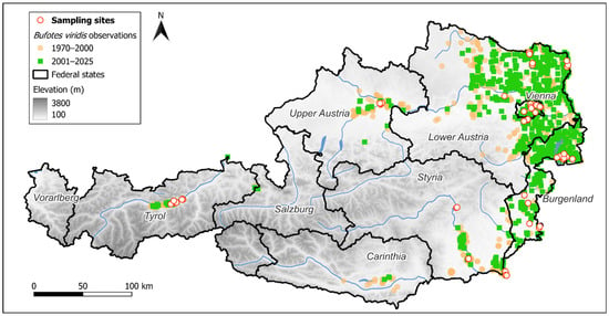
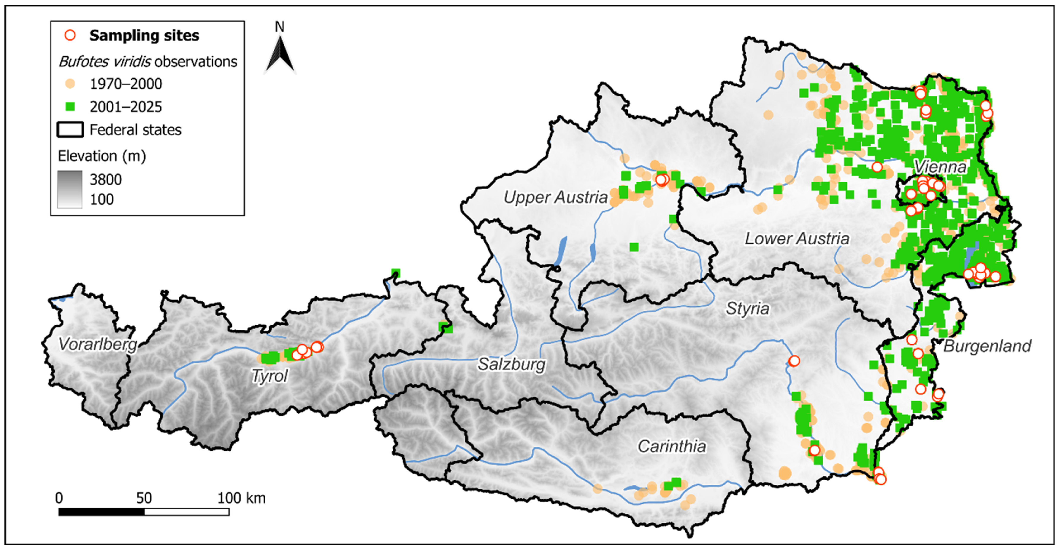
Between April and July 2024, we sampled 68 water bodies throughout Austria (Figure 1). We pre-selected diverse water bodies, varying in characteristics such as size, type, and origin. Since our focus was on the effects of pesticides specifically on small temporary amphibian spawning waters as they are understudied, we chose sites with a known or potential presence of amphibians; we did not consider a priori their location in regard to the surrounding land use. Specifically, we selected potential amphibian spawning habitats situated within the Austrian range of the locally threatened and protected European green toad Bufotes viridis (Laurenti, 1768) (Figure 1), a focal species for our broader research. Green toads mainly occur in lowlands [26]. Typically, adults enter sun-exposed temporary water bodies that lack predatory fish and have sparse vegetation waters to reproduce between April and July, with metamorphosis taking about two months. These natural or man-made waters often occur in the vicinity of arable and urbanized lands. Most of the other 20 Austrian amphibian taxa occur at least partially within the green toad’s range, but they may have different breeding site requirements. Overall, the landscape within the sampled green toad range is representative of the conditions faced by the broader lowland amphibian communities in Austria. Half of the sites (34) were deemed suitable for the reproduction of the green toad, while the other half were suitable for other amphibians but not green toads. These assessments were based on records regarding amphibian presence and reproduction combined from authors’ personal data, the Austrian Herpetofauna Database (HFDÖ)—Natural History Museum Vienna, and iNaturalist.org, as well as on expert knowledge.

Figure 1. Locations of the sampling sites within Austria, compared to recent observations of the European green toad Bufotes viridis (1970–2025). Count of sampling sites per federal state: Burgenland—20; Lower Austria—14; Upper Austria—5; Styria—8; Tyrol—10; Vienna—11. Observations of B. viridis were combined from the Austrian Herpetofauna Database (HFDÖ)—Natural History Museum Vienna and iNaturalist.org.

We visually assessed the characteristics of the water bodies during sampling. We recorded their type and relative size (Table 1), depth and perceived permanence of the water (Table 2). Of the water bodies evaluated, 44 water bodies were man-made (e.g., made of concrete, pond liner, or were the deliberate result of human activity), 12 were semi-natural (potentially created by humans, but then left to natural succession), and 12 were natural. Sixty-six of the water bodies were mostly stagnant and two were flowing. We estimated the elevation above sea level of the water bodies using digital elevation model with pixel size of 10 m and averaging the cell values over a 100 m buffer around the sampling site. The average elevation was 279 m (range 116–846; median = 203).

Table 1. Count of sampled water bodies, by type and size.

	Size (m2)
Type	1–40	41–100	101–1000	>1000	Sum
Pond	3	1	9	12	25
Garden pond	10	4	1		15
Wetland			3	7	10
Puddle	5	2			7
Water drainage	1			2	3
Floodplain			3		3
Fountain		1	1		2
Stream				1	1
Channel				1	1
Lake				1	1
Sum	19	8	17	24	68

Table 2. Count of sampled water bodies, by approximate depth and permanence.

Depth	Temporary	Permanent	Sum
Shallower than 0.3 m	19	3	22
2/3 of water body shallower than 0.3 m, 1/3 deeper	11	3	14
1/3 of water body shallower than 0.3 m, 2/3 deeper	8	8	16
Deeper than 0.3 m	1	15	16
Sum	39	29	68

2.2. Water Sampling and Analysis

For each site the authors took two samples: one at the beginning of the green toad breeding season (8 April–5 June 2024) and another one towards the end of the breeding season (30 June–29 July 2024), with an average of 79 days (range: 54–108; SD = 18.06) between sampling each site. Due to owners’ privacy concerns, we cannot provide specific information on the exact localities.

About 1.25 L of water was collected from the shore, in clean plastic screw-top containers for water samples. Samples were transported in thermo-insulated bags or boxes with ice-cooling elements and were stored at ~5 °C until analysis. The samples were analyzed for 165 pesticides and pesticide metabolites.

Samples were tested in accredited testing laboratories (GEOtest, Brno, Czech Republic) according to ISO 17025:2018. All the methods were accredited and based on specific CSN EN or ISO Norms or EPA methods. Metabolites of herbicides and herbicides were tested using HPLC-MS system according to ISO 21458 for glyphosate and US EOA 535 and US EPA 536 for other herbicides, pesticides and their metabolites. Non-detects were expressed as <LOQ in the test reports. As all the methods are accredited there is always a blank and a quality control sample that is used for regulation diagrams. All the CRMs used for calibration curve and QC were bought and produced in accredited laboratories according to ISO 17034.

Pesticides were classified as herbicides (73), fungicides (30), insecticides (18), metabolites (39), and other substances (5) (Supplementary Table S1). To increase analytical robustness, total concentrations at each site were pooled across both sampling rounds.

2.3. Extracting the Land-Use Data

We obtained the coordinates of the sampling sites using mobile phones’ built-in GPS (accuracy ± 10 m). We then extracted the proportion of the area of each land-use type in a radius around the water body coordinates (Supplementary Table S2). We used four radii: 100 m, 500 m, 2500 m and 5000 m, which enabled us to differentiate between direct contamination routes (e.g., runoff and spills) and long-range transport (e.g., via the air). We used the land-use map of EUSALP LULC [27]. This map is based on the land-use information for the period 2015–2020 and provides a spatial resolution of up to 5 m and overall accuracy of 88.8%. This is the latest available of such data; we consider it adequately represents the land use when samples were taken because we sampled sites that we knew beforehand and they have not changed drastically in the meantime. To simplify classification, we combined all types of arable land, tree cover, water bodies, grasslands, scrubs and woody features each into single categories (changes to the original category labeling are in Supplementary Table S3). The data were obtained using Python (v3.9) with Pandas v2.2.2 [28], Geopandas v1.0.0 [29], Rasterio v1.3.10 [30], Shapely v2.0.6 [31], and NumPy v 2.1.0 [32] libraries.

2.4. Calculating the Pesticide Toxicity

The toxicity of the pesticide’s active ingredients is commonly not tested on amphibian species [23]. Therefore, we used available ecotoxicology data (LC₅₀, LD₅₀ and EC₅₀ values according to their CAS numbers) on other taxa as an approximation for amphibians. We estimated our samples’ pesticide toxicity for birds (“birds—acute”), mammals (mammals—acute oral), aquatic invertebrates (“temperate freshwater aquatic invertebrates—acute 48 h”) and fish (“temperate freshwater fish—acute 96 h”), using the PubChem and The University of Hertfordshire Pesticide Properties databases [33,34]. Birds and mammals were included as they may visit small standing ponds for drinking, while fish and aquatic invertebrates spend most or all of their life in water. Fish were a proxy for amphibians (for which there are no available data), as amphibians spend a significant portion of their life in water and have highly permeable skin. A pesticide’s active ingredients or their metabolites not included in such assessments were disregarded. Toxic load estimation followed Goulson et al. [35], hence, the concentration of substances was divided by their respective LC₅₀, LD₅₀ or EC₅₀ value (whichever was available). Values showing a “higher than” classification were taken at their maximum value to allow calculations.

2.5. Statistics and Plotting

We first reduced the initial 96 predictor variables (24 land-use categories for the four radii, each in percent of the area) using the Boruta algorithm in software R v4.3.2 and RStudio v2023.12.0 [36,37,38]. This approach allows selection of variables with high predictive importance for the response variable in comparison to randomized variables (‘shadow features’). The selected variables were then further challenged in a likelihood-ratio-test (LRT) based model selection approach using the buildmer package v1.5 [39] and generalized linear models with a negative binomial error distribution for pesticide number and the tweedie distribution for all the other responses (using function glm.nb from the MASS package v7.3-65 [40] for the negative binomial model and the function glm and statmod package v1.5.1 for the tweedie distribution [41]). The best model was then tested for multicollinearity using the variance inflation factors (VIF, calculated using the function vif from the car package v3.1-5 for glm [42] and the function check_collinearity of the performance package v0.16.0 [43] for glm.nb); variables with VIF above 5 were excluded from the model. If the LRT model selection already resulted in an intercept-only model, we concluded that the variables did not have a significant influence in generalized linear models on the response variable and did not test any other models. Model checks, after possible VIF variable exclusions, were performed using the function plot (simulateResiduals (model, n = 1000)) from the DHARMa package v0.4.7 [44].

We repeated this approach for each response variable: the number of pesticides, the pesticide concentration, the pesticide toxicity (separately for birds, mammals, aquatic invertebrates and fish). We plotted the Boruta results using the plot method in the Boruta package v9.0.0. Linear predictions were plotted using the ggpredict function in the ggeffects package v2.3.2 [45].

In the case of significant results in one of the reduced models (after VIF check), we tested model validity using a bootstrap approach. For this we created 1000 bootstrapped samples of the original (using the function sample, with replacement) and ran the entire pipeline for each of the generated samples. We then calculated the number of significant results as well as the direction of the effect (sign of the estimate) for each term that appeared in the reduced models (in the bootstrapped samples). This was done to provide an overview of the stability of the overall result and avoid overinterpretation of specific details in the obtained model outputs.

3. Results

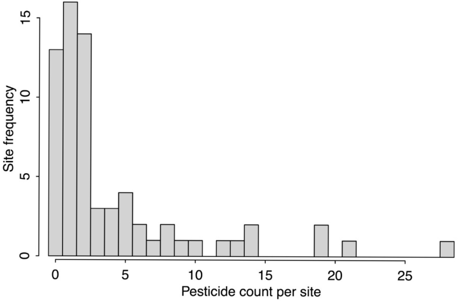
Most sampled sites were relatively small and at least long-term ephemeral: 44 (68%) were less than 1000 m² and 39 (57%) were assessed as fluctuating strongly (up to completely drying up). We detected pesticides in 55 of the 68 sites (81%), with 1 to 28 pesticides per site, including metabolites. Median pooled total pesticide concentration per site was 0.097 µg/L (range: 0–20.419 µg/L).

Out of the 165 pesticides tested for, we detected 54 pesticides and their metabolites. Most were herbicides (25), metabolites (20), and the rest were fungicides (9); we found no insecticides or other substances. The pesticides with the highest concentrations were herbicides, glyphosate being the most prevalent (range: 0–17.43 µg/L). Herbicide presence was dominated by terbuthylazine (desethylterbuthylazine was detected at 23 sites, terbuthylazine-2-hydroxy at 16 and terbuthylazine at 11), metolachlor (metolachlor ethanesulfonic acid was found at 22 sites, metolachlor oxanilic acid at 17 and metolachlor at 10), and glyphosate at 17 sites and the metabolite of glyphosate (aminomethylphosphonic acid, AMPA) was detected at 18 sites.

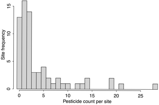
As is typical for count data in natural samples, the results resembled a negative logarithmic function with most of the sites having only a few pesticides detected and a few sites with a very high number of pesticides detected (Figure 2). Pesticides generally co-occurred with their metabolites (e.g., metolachlor with metolachlor oxanilic acid, and glyphosate with AMPA). In addition, when including all metabolites, metolachlor was often associated with terbuthylazine as well as with glyphosate (Supplementary Table S4 for all co-occurrences).

Figure 2. Histogram of detected pesticides and metabolites per water body (55 sites with pesticides, of 68 sampled).

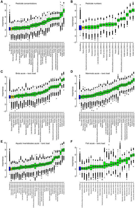
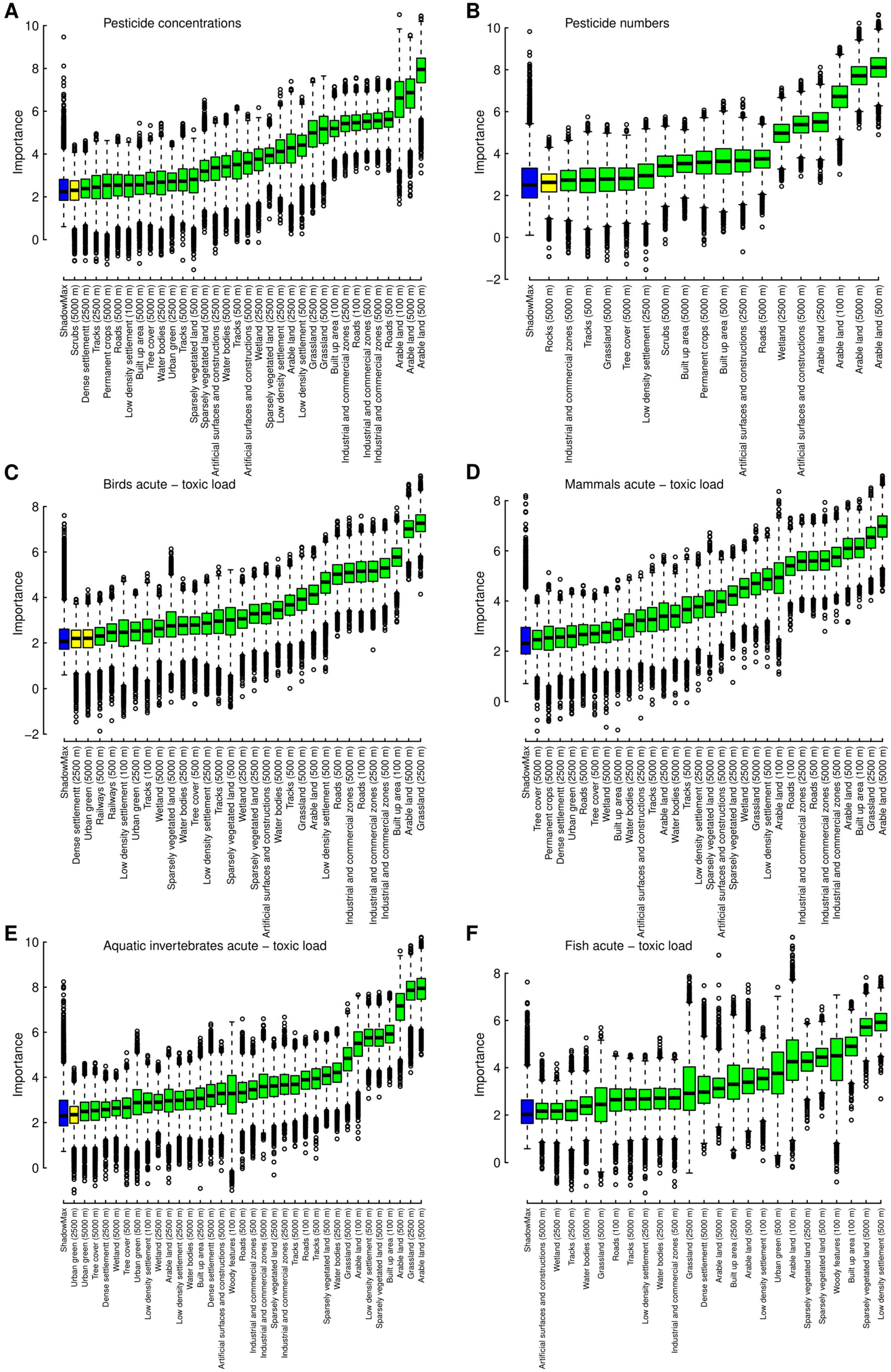
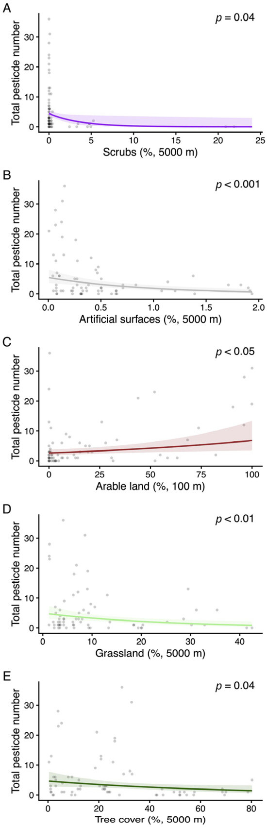
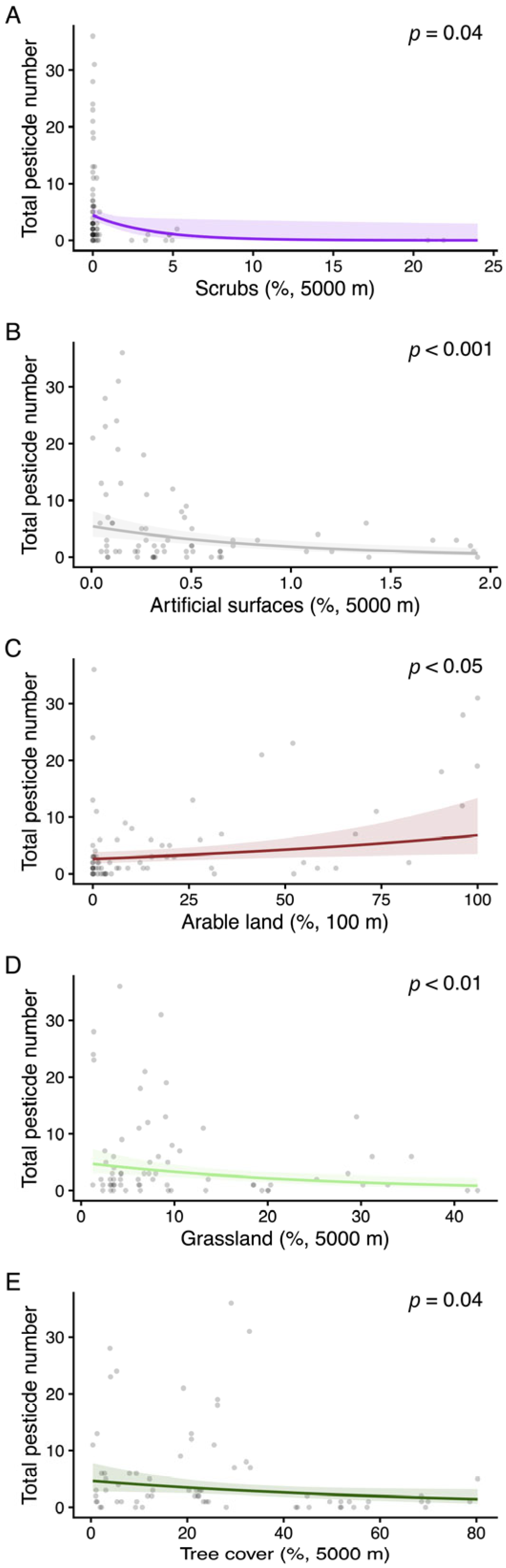
The Boruta analysis showed that arable land at all tested radii around the sample site had a non-random influence on pesticide concentration (Figure 3A and Supplementary Figure S1) and numbers (Figure 3B and Supplementary Figure S1), as well as toxic loads for birds (Figure 3C and Supplementary Figure S2), mammals (Figure 3D and Supplementary Figure S2), aquatic invertebrates (Figure 3E and Supplementary Figure S3) and fish (Figure 3F and Supplementary Figure S3). Pesticides found were generally of lower toxicity, as they were mostly herbicides and in low concentrations. Grassland as well as built-up areas and other artificial surfaces influenced the pesticide occurrence, but not consistently (Figure 3A,B). However, further (linear) model selections showed significant influences of selected parameters only for the number of pesticides (Table 3). The best model for pesticide concentration as well as the toxic loads only included the intercept. The number of pesticides was significantly positively influenced by arable land in a 100 m radius (Table 3 and Figure 4A), but—at the 5000 m radius—negatively by grassland (Figure 4B), artificial surface (Figure 4C), tree cover (Figure 4D) and scrubs (Figure 4E). Model checks did not detect any issues concerning model fit, overdispersion or outliers (see Supplementary Figure S4).

Figure 3. Boruta analysis comparing the possible effects of all land-use parameters including four different radii around the sample sites (100 m, 500 m, 2500 m, 5000 m): Pesticide concentrations (A), number of pesticides (B), and reported toxicity for birds (C) and mammals (D) and aquatic invertebrates (E) and fish (F). Box plots in green are above the chance level when compared to randomized control samples; yellow color indicates a tendency and blue color is the maximum of the shadow features.

Table 3. Best model after linear model selection for total number of pesticides. Observations = 68.

Predictors	Incidence Rate Ratios	CI	p
(Intercept)	13.99	7.20–27.18	<0.001
Scrubs (5000 m)	0.76	0.58–0.99	0.040
Artificial surfaces (5000 m)	0.33	0.19–0.59	<0.001
Arable land (100 m)	1.01	1.00–1.02	0.014
Grassland (5000 m)	0.96	0.93–0.99	0.005
Tree cover (5000 m)	0.99	0.97–1.00	0.041

Figure 4. Results of model predictions for number of pesticides, for scrubs (A), artificial surfaces (B), arable land (C), grassland (D) and tree cover (E). Land-use cover was measured as a percentage (%) of the area in a radius of defined length around the sampling site. Land-use types included in the best model and presented in this figure were either measured in a 5000 m (A,B,D,E) or 100 m radius (C). p-values for the presented effects are shown in each panel. Limits of x-axes depend on the range of the raw data (shown as shaded gray dots) and are therefore different.

Also, the bootstrapping approach for the number of pesticides supported the general trends. Expectedly, it highlighted the variability of such analyses, considering the random sampling (with replacement) to generate the bootstrapped samples. The land-use type scrubs (5000 m radius) was the term most often included and significant in the final models. Furthermore, the first ten terms (ranked after number of times included in the best models) also included artificial surfaces (2500 m and 5000 m), tree cover (100 m, 500 m) and arable land (100 m), but also rocks (5000 m, negative effect) and dense settlement (500 m, negative effect). When ignoring the specific radii, scrubs was significant in 312 models, artificial surfaces in 131, tree cover in 120, arable land in 89 and grassland in 28, while the direction of response of the term was the same as in our real model in 99% (scrubs), 99% (artificial surfaces), 96% (tree cover), 94% (arable land) and 73% (grassland) (see Table S5 for the results sheet). The only effect that was often present in the bootstrap models and with a consistently positive effect on the number of pesticides was arable land. As our pipeline corrects for multicollinearity it had to be expected that certain terms would be replaced or lose significance in some of the bootstrapped results, depending on specific model correlation structures and associations between co-occurring land-use features.

4. Discussion

This is one of the few studies, e.g., [46] that examined pesticide contamination of small temporary water bodies, an essential habitat for amphibians. We focus most of our discussion on amphibians, as we used these organisms to select the sample locations. However, the results should be relevant for other organisms as well, as small standing water bodies are under multiple pressures, while being highly important for biodiversity in general [47].

Arable land was the predominant land-use type associated with pesticide occurrence; the Boruta analysis identified it as important for all response variables analyzed. However, our generalized linear modeling approach showed that only the number of pesticides was significantly positively affected by (nearby) arable land. This indicates that the detected pesticide concentrations and the resulting toxicity values were more variable than the number of pesticides, as would be expected in such samples. Presence is easier to detect than precise concentrations, especially when the concentrations are generally low, as in our study. Similarly, a recent Belgian study found no correlation of pesticide concentration in amphibian breeding ponds and agricultural land [24]. In contrast to our results, they also did not find a correlation between numbers of contaminants and agricultural land. These combined results indicate that a failed detection of such correlations is likely due to a lack of statistical power and is not evidence for lack of association. Hence, we recommend that studies correlating pesticide concentration to land should aim to carry out a priori power analysis when planning sampling.

Given that agricultural practices are the main source of pesticides, this difference between number and concentration suggests that pesticide drift is influenced by external factors such as runoff, soil type, local hydrodynamics, or weather conditions like sun exposure, wind, rain and temperature [48], leading to quite different concentrations at equal distances to the source [10,49]. Such effects could largely increase the variability of concentration in contrast to mere number of pesticides, making it harder to model concentrations at different scales. Specific agricultural practices related to the timing of pesticide application might also influence results. However, such effects were likely not relevant in our study as the two samples were pooled to avoid possible temporal influences. Interestingly, there was no clear trend indicating that arable land closer to water bodies was a better predictor of pesticide concentration, number or toxic load than arable land further away. However, given the high variability of our data set pesticides occurrence may still be negatively correlated with distance to arable land, it is clear that further studies to test such potential correlations would be needed.

The influence of arable land presence on pesticide numbers likely means that cocktail effects, e.g., increased toxicity of the combined harmful substances compared to their individual toxicity [50] are more likely to be an issue in the vicinity of arable land [51], especially if combined with fertilizers. Furthermore, while the predominant pesticides were herbicides at relatively low levels and low toxicity to animals [52], it would be important to study the effects of common pesticide mixtures in ecotoxicological experiments. Such possible effects are largely understudied [53,54]. Studying chemical cocktails is also relevant, as often multiple active substances are mixed in a single commercial pesticide product [52]. Other synergistic effects with environmental stressors (e.g., extreme temperatures, rapid changes in water level, sun exposure, food availability) should also be considered, but are complex to model [55].

It is important to note that, with the approach used in this study, toxicity levels should be seen as relative estimates, especially as assessments on our target taxa (amphibians) are unavailable. Depending on multiple factors, an individual might be exposed to lower or higher concentrations that could be sub-lethal but still harmful, including due to ontogenetic shifts in physiology, behavior, and diet, time of arrival at the aquatic habitat after pollution event, and duration of exposure. Additionally, only water sampling might not capture all pesticides present, as some are captured in biofilms, exposing organisms through dietary pathways [56].

Furthermore, we stress that we have analyzed only pesticides as one type of contaminant affecting amphibian spawning waters. In urban areas, pharmaceuticals, heavy metals, and acidity have been identified as toxicological threats to amphibians [57,58,59]. Such pollutants from non-agriculture related pathways might be present in waters that are free of pesticides, including those in our study.

Although amphibians are highly endangered and are especially susceptible to pollutants because of their complex life cycle and their permeable skin, ecotoxicological research on amphibians remains scarce [60,61]. Especially amphibians that are, at least at times, associated with agricultural land, such as populations of the green toad, the common toad Bufo bufo (Linnaeus, 1758) and the spadefoot toad Pelobates fuscus (Laurenti, 1768), might be exposed to considerably higher levels than forest-inhabiting individuals. Individuals may also migrate across contaminated soil on their way to their spawning grounds [62,63]. Direct terrestrial pesticide exposure should also be considered [64]. In any case, given their life history and strong association with water bodies and their surrounding habitats (including agricultural land), amphibians are likely to stay in potentially pesticide-exposed habitats for long time (larval and adult life), thus short fluctuations might be less important than overall pesticide numbers and concentrations [65,66]. This makes them a suitable bioindicator species for environmental quality on the one hand and highlights the importance of including small standing water bodies to monitoring activities of pesticides in aquatic systems. In this study, we show a considerable number of pesticides present in such water bodies and provide a basis to design further experiments for broader biomonitoring schemes, including small and ephemeral standing waters harboring diverse animal communities.

5. Conclusions

Pesticides are common pollutants in smaller ephemeral water bodies, which are typical spawning habitats of amphibians. The main driver of pesticide presence appears to be proximity to arable land. Studies correlating pesticide concentration to land use should aim to carry out a priori power analysis when planning sampling. However, while pesticide concentration is very variable the number of pesticides (how many different pesticide compounds are found) is significantly related to the arable land in the vicinity of the water bodies. Therefore, it would be necessary to consider potential cocktail effects in laboratory studies examining the toxicity of pesticides on animals, especially amphibians. Long-term bioaccumulation of pollutants by amphibians utilizing small water bodies and/or timing of pesticides release in the environment in relation to the amphibians’ life cycle should also be considered. Our results emphasize the need for small and ephemeral standing waters, harboring diverse animal communities, to be included in biomonitoring schemes, testing for pesticides and other contaminants affecting the biodiversity, to affect environmental monitoring and risk assessments.

References

- Elhamalawy, O.; Bakr, A.; Eissa, F. Impact of Pesticides on Non-Target Invertebrates in Agricultural Ecosystems. Pestic. Biochem. Physiol. 2024, 202, 105974. [Google Scholar] [CrossRef] [Scilit] [PubMed]
- Etterson, M.; Garber, K.; Odenkirchen, E. Mechanistic Modeling of Insecticide Risks to Breeding Birds in North American Agroecosystems. PLoS ONE 2017, 12, e0176998. [Google Scholar] [CrossRef] [Scilit]
- Mauser, K.M.; Brühl, C.A.; Zaller, J.G. Herbicide Effects on Nontarget Organisms, Biodiversity and Ecosystem Functions. In Encyclopedia of Biodiversity; Elsevier: Amsterdam, The Netherlands, 2024; pp. 239–257. [Google Scholar]
- Strandberg, B.; Boutin, C.; Mathiassen, S.K.; Damgaard, C.; Dupont, Y.L.; Carpenter, D.J.; Kudsk, P. Effects of Herbicides on Non-Target Terrestrial Plants. In ACS Symposium Series; Duke, S.O., Kudsk, P., Solomon, K., Eds.; American Chemical Society: Washington, DC, USA, 2017; Volume 1249, pp. 149–166. [Google Scholar]
- Albaseer, S.S.; Jaspers, V.L.B.; Orsini, L.; Vlahos, P.; Al-Hazmi, H.E.; Hollert, H. Beyond the Field: How Pesticide Drift Endangers Biodiversity. Environ. Pollut. 2025, 366, 125526. [Google Scholar] [CrossRef] [Scilit]
- Daam, M.A.; Van Den Brink, P.J. Risk Assessment of Agrochemicals on Irrigation Water Quality. Acta Hortic. 2011, 41–47. [Google Scholar] [CrossRef] [Scilit]
- El Afandi, G.; Ismael, H.; Fall, S. Application of OpenAir and AgDRIFT Models to Estimate Organophosphate Pesticide Spray Drift: A Case Study in Macon County, Alabama. Agriculture 2023, 13, 1763. [Google Scholar] [CrossRef] [Scilit]
- Lee, S.-J.; Mehler, L.; Beckman, J.; Diebolt-Brown, B.; Prado, J.; Lackovic, M.; Waltz, J.; Mulay, P.; Schwartz, A.; Mitchell, Y.; et al. Acute Pesticide Illnesses Associated with Off-Target Pesticide Drift from Agricultural Applications: 11 States, 1998–2006. Environ. Health Perspect. 2011, 119, 1162–1169. [Google Scholar] [CrossRef] [Scilit]
- Liess, M.; Liebmann, L.; Vormeier, P.; Weisner, O.; Altenburger, R.; Borchardt, D.; Brack, W.; Chatzinotas, A.; Escher, B.; Foit, K.; et al. Pesticides Are the Dominant Stressors for Vulnerable Insects in Lowland Streams. Water Res. 2021, 201, 117262. [Google Scholar] [CrossRef] [Scilit]
- Zaller, J.G.; Kruse-Plaß, M.; Schlechtriemen, U.; Gruber, E.; Peer, M.; Nadeem, I.; Formayer, H.; Hutter, H.-P.; Landler, L. Pesticides in Ambient Air, Influenced by Surrounding Land Use and Weather, Pose a Potential Threat to Biodiversity and Humans. Sci. Total Environ. 2022, 838, 156012. [Google Scholar] [CrossRef] [Scilit]
- Brühl, C.A.; Zaller, J.G. Biodiversity Decline as a Consequence of an Inappropriate Environmental Risk Assessment of Pesticides. Front. Environ. Sci. 2019, 7, 177. [Google Scholar] [CrossRef] [Scilit]
- Solé, M.; Brendel, S.; Aldrich, A.; Dauber, J.; Ewald, J.; Duquesne, S.; Gottschalk, E.; Hoffmann, J.; Kuemmerlen, M.; Leake, A.; et al. Assessing In-Field Pesticide Effects under European Regulation and Its Implications for Biodiversity: A Workshop Report. Environ. Sci. Eur. 2024, 36, 153. [Google Scholar] [CrossRef] [Scilit]
- Peresin, D.; Bortolin, T.A.; Chiarelo, M.; Moura E Silva, S.; Magro, T.D.; Menegat, D.; Schneider, V.E. Analysis of the Concentration of Pesticides in a Watershed for Public Water Supply in Brazil. Sustain. Water Resour. Manag. 2023, 9, 57. [Google Scholar] [CrossRef] [Scilit]
- San Juan, M.R.F.; Lavarías, S.M.L.; Aparicio, V.; Larsen, K.E.; Lerner, J.E.C.; Cortelezzi, A. Ecological Risk Assessment of Pesticides in Sediments of Pampean Streams, Argentina. Chemosphere 2023, 313, 137598. [Google Scholar] [CrossRef] [Scilit]
- Wang, D.; Singhasemanon, N.; Goh, K.S. A Statistical Assessment of Pesticide Pollution in Surface Waters Using Environmental Monitoring Data: Chlorpyrifos in Central Valley, California. Sci. Total Environ. 2016, 571, 332–341. [Google Scholar] [CrossRef] [Scilit]
- Speybroeck, J.; Beukema, W.; Bok, B.; Van Der Voort, J.; Velikov, I. Field Guide to the Amphibians and Reptiles of Britain and Europe; Bloomsbury Publishing: London, UK, 2016. [Google Scholar]
- Lenhardt, P.P.; Brühl, C.A.; Berger, G. Temporal Coincidence of Amphibian Migration and Pesticide Applications on Arable Fields in Spring. Basic Appl. Ecol. 2015, 16, 54–63. [Google Scholar] [CrossRef] [Scilit]
- Quaranta, A.; Bellantuono, V.; Cassano, G.; Lippe, C. Why Amphibians Are More Sensitive than Mammals to Xenobiotics. PLoS ONE 2009, 4, e7699. [Google Scholar] [CrossRef] [Scilit]
- Milošković, A.; Đuretanović, S.; Radenković, M.; Kojadinović, N.; Veličković, T.; Milošević, Đ.; Simić, V. Pollution of Small Lakes and Ponds of the Western Balkans—Assessment of Levels of Potentially Toxic Elements. In Small Water Bodies of the Western Balkans; Pešić, V., Milošević, D., Miliša, M., Eds.; Springer: Cham, Switzerland, 2022; pp. 419–435. [Google Scholar]
- Ulrich, U.; Hörmann, G.; Unger, M.; Pfannerstill, M.; Steinmann, F.; Fohrer, N. Lentic Small Water Bodies: Variability of Pesticide Transport and Transformation Patterns. Sci. Total Environ. 2018, 618, 26–38. [Google Scholar] [CrossRef] [Scilit] [PubMed]
- Luedtke, J.A.; Chanson, J.; Neam, K.; Hobin, L.; Maciel, A.O.; Catenazzi, A.; Borzée, A.; Hamidy, A.; Aowphol, A.; Jean, A.; et al. Ongoing Declines for the World’s Amphibians in the Face of Emerging Threats. Nature 2023, 622, 308–314. [Google Scholar] [CrossRef] [Scilit]
- Mann, R.M.; Hyne, R.V.; Choung, C.B.; Wilson, S.P. Amphibians and Agricultural Chemicals: Review of the Risks in a Complex Environment. Environ. Pollut. 2009, 157, 2903–2927. [Google Scholar] [CrossRef] [Scilit]
- Brühl, C.A.; Pieper, S.; Weber, B. Amphibians at Risk? Susceptibility of Terrestrial Amphibian Life Stages to Pesticides. Environ. Toxicol. Chem. 2011, 30, 2465–2472. [Google Scholar] [CrossRef] [Scilit] [PubMed]
- Goessens, T.; De Baere, S.; Deknock, A.; De Troyer, N.; Van Leeuwenberg, R.; Martel, A.; Pasmans, F.; Goethals, P.; Lens, L.; Spanoghe, P.; et al. Agricultural Contaminants in Amphibian Breeding Ponds: Occurrence, Risk and Correlation with Agricultural Land Use. Sci. Total Environ. 2022, 806, 150661. [Google Scholar] [CrossRef] [Scilit]
- Eurostat Agri-Environmental Indicator—Consumption of Pesticides. Available online: https://ec.europa.eu/eurostat/statistics-explained/index.php?title=Agri-environmental_indicator_-_consumption_of_pesticides (accessed on 21 November 2025).
- Stöck, M.; Roth, P.; Podloucky, R.; Grossenbacher, K. Wechselkröten—Unter Berücksichtigung von Bufo viridis virdis Laurenti, 1768; Bufo variabilis (Pallas, 1769); Bufo boulengeri Lataste, 1879; Bufo balearicus Böttger, 1880 Und Bufo siculus Stöck, Sicilia, Belfiore, Lo Brutto, Lo Valvo Und Arculeo, 2008. In Handbuch der Reptilien und Amphibien Europas; Aula-Verlag: Wiesbaden, Germany, 2008; pp. 413–498. [Google Scholar]
- Marsoner, T.; Simion, H.; Giombini, V.; Egarter Vigl, L.; Candiago, S. A Detailed Land Use/Land Cover Map for the European Alps Macro Region. Sci. Data 2023, 10, 468. [Google Scholar] [CrossRef] [Scilit]
- McKinney, W. Data Structures for Statistical Computing in Python. SciPy 2010, 445, 51–56. [Google Scholar]
- Jordahl, K.; Bossche, J.V.; Fleischmann, M.; Wasserman, J.; McBride, J.; Gerard, J.; Tratner, J.; Perry, M.; Badaracco, A.G.; Farmer, C.; et al. Geopandas/Geopandas, v1.0.0; Zenodo: Geneva, Switzerland, 2020. [CrossRef]
- Gillies, S. Rasterio: Geospatial Raster I/O for Python Programmers 2013, Mapbox. Available online: https://github.com/rasterio/rasterio (accessed on 11 December 2025).
- Gillies, S.; Wel, C.; Van den Bossche, J.; Taves, M.W.; Arnott, J.; Ward, B.C. Shapely, Version 2.0.6; Zenodo: Geneva, Switzerland, 2022. [CrossRef]
- Harris, C.R.; Millman, K.J.; Van Der Walt, S.J.; Gommers, R.; Virtanen, P.; Cournapeau, D.; Wieser, E.; Taylor, J.; Berg, S.; Smith, N.J.; et al. Array Programming with NumPy. Nature 2020, 585, 357–362. [Google Scholar] [CrossRef] [Scilit] [PubMed]
- Kim, S.; Chen, J.; Cheng, T.; Gindulyte, A.; He, J.; He, S.; Li, Q.; Shoemaker, B.A.; Thiessen, P.A.; Yu, B.; et al. PubChem 2025 Update. Nucleic Acids Res. 2025, 53, D1516–D1525. [Google Scholar] [CrossRef] [Scilit]
- Lewis, K.A.; Tzilivakis, J.; Warner, D.J.; Green, A. An International Database for Pesticide Risk Assessments and Management. Hum. Ecol. Risk Assess. Int. J. 2016, 22, 1050–1064. [Google Scholar] [CrossRef] [Scilit]
- Goulson, D.; Thompson, J.; Croombs, A. Rapid Rise in Toxic Load for Bees Revealed by Analysis of Pesticide Use in Great Britain. PeerJ 2018, 6, e5255. [Google Scholar] [CrossRef] [Scilit]
- Kursa, M.B.; Rudnicki, W.R. Feature Selection with the Boruta Package. J. Stat. Softw. 2010, 36, 1–13. [Google Scholar] [CrossRef] [Scilit]
- Posit Team RStudio. Integrated Development Environment for R 2025, Posit Software, PBC: Boston, MA, USA, 2025. Available online: http://www.posit.co/ (accessed on 11 December 2025).
- R Core Team R. A Language and Environment for Statistical Computing 2025, R Foundation for Statistical Computing: Vienna, Austria, 2025. Available online: https://www.R-project.org/ (accessed on 11 December 2025).
- Voeten, C.C. Buildmer: Stepwise Elimination and Term Reordering for Mixed-Effects Regression 2020, R Package Version 1.5. Available online: https://CRAN.R-project.org/package=buildmer (accessed on 11 December 2025).
- Venables, W.N.; Ripley, B.D. Modern Applied Statistics with S, 4th ed.; Springer: New York, NY, USA, 2002. [Google Scholar]
- Dunn, P.K.; Smyth, G.K. Generalized Linear Models with Examples in R; Springer Texts in Statistics; Springer: New York, NY, USA, 2018. [Google Scholar]
- Fox, J.; Weisberg, S. An R Companion to Applied Regression, 3rd ed.; Sage: Thousand Oaks, CA, USA, 2019. [Google Scholar]
- Lüdecke, D.; Ben-Shachar, M.; Patil, I.; Waggoner, P.; Makowski, D. Performance: An R Package for Assessment, Comparison and Testing of Statistical Models. J. Open Source Softw. 2021, 6, 3139. [Google Scholar] [CrossRef] [Scilit]
- Hartig, F. DHARMa: Residual Diagnostics for Hierarchical (Multi-Level/Mixed) Regression Models 2024, Version 0.4.7. Available online: https://CRAN.R-project.org/package=DHARMa (accessed on 11 December 2025).
- Lüdecke, D. ggeffects: Tidy Data Frames of Marginal Effects from Regression Models. J. Open Source Softw. 2018, 3, 772. [Google Scholar] [CrossRef] [Scilit]
- Navarro, I.; De La Torre, A.; Sanz, P.; Abrantes, N.; Campos, I.; Alaoui, A.; Christ, F.; Alcon, F.; Contreras, J.; Glavan, M.; et al. Assessing Pesticide Residues Occurrence and Risks in Water Systems: A Pan-European and Argentina Perspective. Water Res. 2024, 254, 121419. [Google Scholar] [CrossRef] [Scilit] [PubMed]
- IGB. Small Standing Water Bodies as Biodiversity Hotspots—Particularly Valuable, but Highly Endangered. Options for Action, Protection and Restoration; IGB Dossier; Leibniz Institute of Freshwater Ecology and Inland Fisheries: Berlin, Germany, 2023. [Google Scholar]
- Linhart, C.; Niedrist, G.H.; Nagler, M.; Nagrani, R.; Temml, V.; Bardelli, T.; Wilhalm, T.; Riedl, A.; Zaller, J.G.; Clausing, P.; et al. Pesticide Contamination and Associated Risk Factors at Public Playgrounds near Intensively Managed Apple and Wine Orchards. Environ. Sci. Eur. 2019, 31, 28. [Google Scholar] [CrossRef] [Scilit]
- Thomson, S.J.; Huang, Y. Comparison of Weather Acquisition Periods Influencing a Statistical Model of Aerial Pesticide Drift. Agronomy 2023, 13, 213. [Google Scholar] [CrossRef] [Scilit]
- Rizzati, V.; Briand, O.; Guillou, H.; Gamet-Payrastre, L. Effects of Pesticide Mixtures in Human and Animal Models: An Update of the Recent Literature. Chem. Biol. Interact. 2016, 254, 231–246. [Google Scholar] [CrossRef] [Scilit]
- Mauser, K.M.; Wolfram, J.; Spaak, J.W.; Honert, C.; Brühl, C.A. Current-Use Pesticides in Vegetation, Topsoil and Water Reveal Contaminated Landscapes of the Upper Rhine Valley, Germany. Commun. Earth Environ. 2025, 6, 166. [Google Scholar] [CrossRef] [Scilit]
- Mesnage, R.; Zaller, J.G. (Eds.) Herbicides: Chemistry, Efficacy, Toxicology, and Environmental Impacts; Elsevier: Amsterdam, The Netherlands, 2021. [Google Scholar]
- Cairo, M.; Monnet, A.-C.; Robin, S.; Porcher, E.; Fontaine, C. Identifying Pesticide Mixtures at Country-Wide Scale. Peer Community J. 2024, 4, e100. [Google Scholar] [CrossRef] [Scilit]
- Schemmer, A.; Wolfram, J.; Roodt, A.P.; Bub, S.; Petschick, L.L.; Herrmann, L.Z.; Stehle, S.; Schulz, R. Pesticide Mixtures in Surface Waters of Two Protected Areas in Southwestern Germany. Bull. Environ. Contam. Toxicol. 2024, 112, 10. [Google Scholar] [CrossRef] [Scilit]
- Liess, M.; Henz, S.; Shahid, N. Modeling the Synergistic Effects of Toxicant Mixtures. Environ. Sci. Eur. 2020, 32, 119. [Google Scholar] [CrossRef] [Scilit]
- Izma, G.; Raby, M.; Prosser, R.; Rooney, R. Urban-Use Pesticides in Stormwater Ponds and Their Accumulation in Biofilms. Sci. Total Environ. 2024, 918, 170534. [Google Scholar] [CrossRef] [Scilit]
- Croteau, M.C.; Hogan, N.; Gibson, J.C.; Lean, D.; Trudeau, V.L. Toxicological Threats to Amphibians and Reptiles in Urban Environments. In Urban Herpetology; Mitchell, J.C., Brown, R.E.J., Bartholomew, B., Eds.; Herpetological Conservation; Society for the Study of Amphibians and Reptiles: Ann Arbor, MI, USA, 2008; Volume 3, pp. 197–209. [Google Scholar]
- Lemaire, J.; Mangione, R.; Spießberger, M.; Burgstaller, S.; Staufer, M.; Gruber, E.; Zaller, J.G.; Bustamante, P.; Landler, L. Mercury Contamination in the European Green Toad Bufotes viridis in Vienna, Austria. Ecotoxicol. Environ. Saf. 2025, 292, 117957. [Google Scholar] [CrossRef] [Scilit]
- Zaller, J.G.; Kruse-Plaß, M.; Schlechtriemen, U.; Gruber, E.; Peer, M.; Nadeem, I.; Formayer, H.; Hutter, H.-P.; Landler, L. Unexpected Air Pollutants with Potential Human Health Hazards: Nitrification Inhibitors, Biocides, and Persistent Organic Substances. Sci. Total Environ. 2023, 862, 160643. [Google Scholar] [CrossRef] [Scilit] [PubMed]
- Egea-Serrano, A.; Relyea, R.A.; Tejedo, M.; Torralva, M. Understanding of the Impact of Chemicals on Amphibians: A Meta-analytic Review. Ecol. Evol. 2012, 2, 1382–1397. [Google Scholar] [CrossRef] [Scilit] [PubMed]
- Langlois, V.S. Amphibian Toxicology: A Rich but Underappreciated Model for Ecotoxicology Research. Arch. Environ. Contam. Toxicol. 2021, 80, 661–662. [Google Scholar] [CrossRef] [Scilit] [PubMed]
- Froger, C.; Jolivet, C.; Budzinski, H.; Pierdet, M.; Caria, G.; Saby, N.P.A.; Arrouays, D.; Bispo, A. Pesticide Residues in French Soils: Occurrence, Risks, and Persistence. Environ. Sci. Technol. 2023, 57, 7818–7827. [Google Scholar] [CrossRef] [Scilit]
- Silva, V.; Mol, H.G.J.; Zomer, P.; Tienstra, M.; Ritsema, C.J.; Geissen, V. Pesticide Residues in European Agricultural Soils—A Hidden Reality Unfolded. Sci. Total Environ. 2019, 653, 1532–1545. [Google Scholar] [CrossRef] [Scilit]
- Brühl, C.A.; Schmidt, T.; Pieper, S.; Alscher, A. Terrestrial Pesticide Exposure of Amphibians: An Underestimated Cause of Global Decline? Sci. Rep. 2013, 3, 1135. [Google Scholar] [CrossRef] [Scilit]
- Leeb, C.; Brühl, C.; Theissinger, K. Potential Pesticide Exposure during the Post-Breeding Migration of the Common Toad (Bufo bufo) in a Vineyard Dominated Landscape. Sci. Total Environ. 2020, 706, 134430. [Google Scholar] [CrossRef] [Scilit]
- Leeb, C.; Kolbenschlag, S.; Laubscher, A.; Adams, E.; Brühl, C.A.; Theissinger, K. Avoidance Behavior of Juvenile Common Toads (Bufo bufo) in Response to Surface Contamination by Different Pesticides. PLoS ONE 2020, 15, e0242720. [Google Scholar] [CrossRef] [Scilit] [PubMed]
Disclaimer/Publisher’s Note: The statements, opinions and data contained in all publications are solely those of the individual author(s) and contributor(s) and not of MDPI and/or the editor(s). MDPI and/or the editor(s) disclaim responsibility for any injury to people or property resulting from any ideas, methods, instructions or products referred to in the content. |
© 2026 by the authors. Licensee MDPI, Basel, Switzerland. This article is an open access article distributed under the terms and conditions of the Creative Commons Attribution (CC BY) license.