


Abstract
To improve the accuracy of predicting photosynthetic rates of protected grapes, a protected grape photosynthetic rate prediction model based on the improved grey wolf optimization (IGWO) algorithm is proposed in this paper. Shine Muscat and Nina Queen protected grapes were taken as research subjects, and photosynthetic data of both grape varieties were first collected. Through key feature selection, environmental parameters—photosynthetic photon flux density, air temperature, relative humidity, carbon dioxide concentration, and light quality—were selected as model inputs. Subsequently, the back propagation (BP) neural network model was optimized using the grey wolf optimization (GWO) algorithm. Chaotic mapping and a nonlinear decreasing cosine function were introduced to enhance global and local search capabilities, leading to the construction of an improved IGWO-BP-based protected grapes photosynthetic rate prediction model. The model was validated using a biological-replicate-level independent dataset splitting strategy to avoid information leakage. Preliminary tests on the conventional BP revealed its limitations: it easily falls into local optima and exhibits poor stability when fitting grape photosynthetic data. The results of 10 independent repeated experiments showed that the IGWO-BP model significantly improved prediction accuracy, stability and out-of-sample performance. The average coefficient of determination (R2) of the overall sample test set reached 0.990, with the average mean absolute error (MAE) reduced by 58.0% compared with the traditional BP model and by 24.6% compared with the GWO-BP model; the average mean squared error (MSE) was decreased by 81.8% compared with the traditional BP model and by 43.6% compared with the GWO-BP model; and the average root mean square error (RMSE) was reduced by 57.4% compared with the traditional BP model and by 24.9% compared with the GWO-BP model. The improved IGWO-BP model can achieve high-accuracy prediction of protected grape photosynthetic rate.
1. Introduction
Protected cultivation refers to an agricultural production mode that uses facilities such as solar greenhouses, multi-span greenhouses and plastic tunnels to artificially regulate environmental factors (light, temperature, humidity, CO2 concentration, etc.), so as to break the restrictions of natural climate conditions on crop growth. For grape cultivation, protected facilities can not only realize off-season production and expand planting areas but also precisely regulate the ecophysiological processes of grapes such as photosynthesis, transpiration, stomatal movement and dry matter accumulation, so as to significantly improve fruit yield and quality [1].
Photosynthesis is the core physiological process for the accumulation of substances and the formation of quality in protected grapes, and the photosynthetic rate directly determines crop yield and economic benefits [2]. Accurate prediction of the photosynthetic rate is a key technical support for achieving intelligent regulation of the protected environment and optimizing resource allocation. Research on the prediction of photosynthetic rates in protected grapes can fill the gaps in existing models regarding adaptation to complex environments, provide a scientific basis for high-quality and high-yield grape production in protected cultivation and hold important practical significance for promoting the precision and intelligent development of protected agriculture [3,4].
Machine learning has been widely adopted for crop photosynthesis prediction in recent years. LI-RBF neural networks have been used for protected crop photosynthesis estimation, but inputs were restricted to temperature, humidity, photosynthetic photon flux density and CO2 concentration without considering light quality [5]. BP neural networks for tomato photosynthesis captured CO2–soil moisture interactions to realize multi-stage prediction, yet only light and temperature were included as environmental predictors [6]. Levenberg–Marquardt optimized BP models have reduced training error in cucumber photosynthesis forecasting [7]. These studies developed machine learning models for protected crop photosynthesis, but most models only adopt conventional environmental inputs such as temperature, light and humidity. Research on protected grape photosynthesis prediction models incorporating light quality remains limited.
Among existing machine learning methods, the BP neural network is selected as the base prediction model in the present study for solid theoretical and practical reasons. The response relationship between environmental factors and crop photosynthetic rate presents typical nonlinear, multi-factor coupling features, and the BP neural network has strong nonlinear fitting ability, which can effectively approximate the complex mapping between multiple input variables and output targets without relying on explicit mechanistic equations [8].
The present study introduces the GWO to optimize the initial parameters of a BP network. The GWO is chosen as the optimization framework mainly based on the following considerations: first, compared with gradient-based optimization methods, GWO as a meta-heuristic algorithm does not depend on the differentiability of the objective function, which is suitable for optimizing the weight parameters of neural networks with nonconvex loss landscapes; second, GWO has the advantages of few adjustable parameters, simple implementation and strong global search ability, which has been widely verified in agricultural parameter optimization scenarios; third, the social hierarchy mechanism of GWO can balance exploration and exploitation in the search process, which has natural advantages for solving the premature convergence problem of BP network training [9].
Quantum-inspired algorithms have been compared with standard GWO for the prediction of soil hydraulic conductivity; quantum-inspired approaches reduced prediction errors by 37–42% in fine-textured soils relative to conventional methods [10]. Adaptive GWO variants have been implemented to optimize maize field management, delivering a 50% improvement in crop yield and economic profit [11]. GWO has also been employed for multi-objective planting-structure optimization in irrigated regions to generate solutions balancing resource, economic and social benefits [12]. Improved GWO-based intelligent optimization frameworks have been developed for coordinated water–nitrogen management, raising water and nitrogen use efficiencies by 18.69% and 21.83%, respectively [13]. Hybrid models integrating GWO with kernel ridge regression have been built to estimate wheat yield from satellite observations, reducing prediction errors by approximately 20% [14]. These studies demonstrate that GWO and its improved variants exhibit good applicability and effectiveness in various agricultural scenarios. However, the original GWO still suffers from the drawback of easily falling into local optima when dealing with complex agricultural physiological data characterized by high nonlinearity and multiple interacting factors, which limits further improvement in model prediction performance. Therefore, enhancing GWO or integrating it with other strategies tailored to the features of agricultural data has become an important research direction.
In this study, multiple environmental and physiological variables were collected for protected grape leaves. The measured candidate environmental variables include photosynthetic photon flux density, air temperature, relative humidity, carbon dioxide concentration, light quality, leaf-chamber temperature and gas flow rate. For the machine learning workflow, this work employs BP neural network structural parameters (input/hidden/output-layer neuron counts), trainable weights and thresholds, as well as training hyper-parameters including batch size, activation function and optimizer. The IGWO algorithm involves swarm population size, maximum iteration number, Tent chaotic mapping coefficient and nonlinear cosine-form convergence factor.
Despite the existing research progress, three core research gaps still remain in the field of protected grape photosynthetic rate prediction: (1) factor gap: most existing photosynthetic rate prediction models only consider conventional environmental factors such as temperature, light intensity and humidity and rarely incorporate light quality features into the prediction model for protected grapes [5]. (2) Algorithm gap: the GWO, which is widely used in agricultural modeling, is prone to premature convergence to local optima when processing complex photosynthetic data, resulting in model stability and generalization ability that cannot meet the needs of precise environmental regulation [9]. (3) Applicability gap: there is still a lack of photosynthetic rate prediction models specifically for protected grape varieties that can cover full light intensity gradients and multiple light quality conditions [4].
The present study proposes the following research hypotheses: (1) introducing light quality as an input factor can effectively improve the prediction accuracy of the grape photosynthetic rate model; (2) improving the population initialization strategy and convergence factor adjustment mechanism of the GWO can alleviate the premature convergence problem and enhance the model’s prediction performance.
The aims of this study were: (1) to construct an input system for protected grape photosynthetic rate prediction that incorporates light quality factors, to compensate for the limitation of traditional models ignoring spectral regulatory effects; (2) to propose an IGWO integrating Tent chaotic mapping and nonlinear cosine convergence factor, to mitigate the premature convergence problem of standard GWO; (3) to compare the prediction performance of the developed IGWO-BP model with conventional BP and GWO-BP models.
2. Materials and Methods
2.1. Experimental Subjects and Data Collection
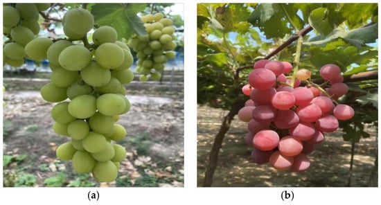
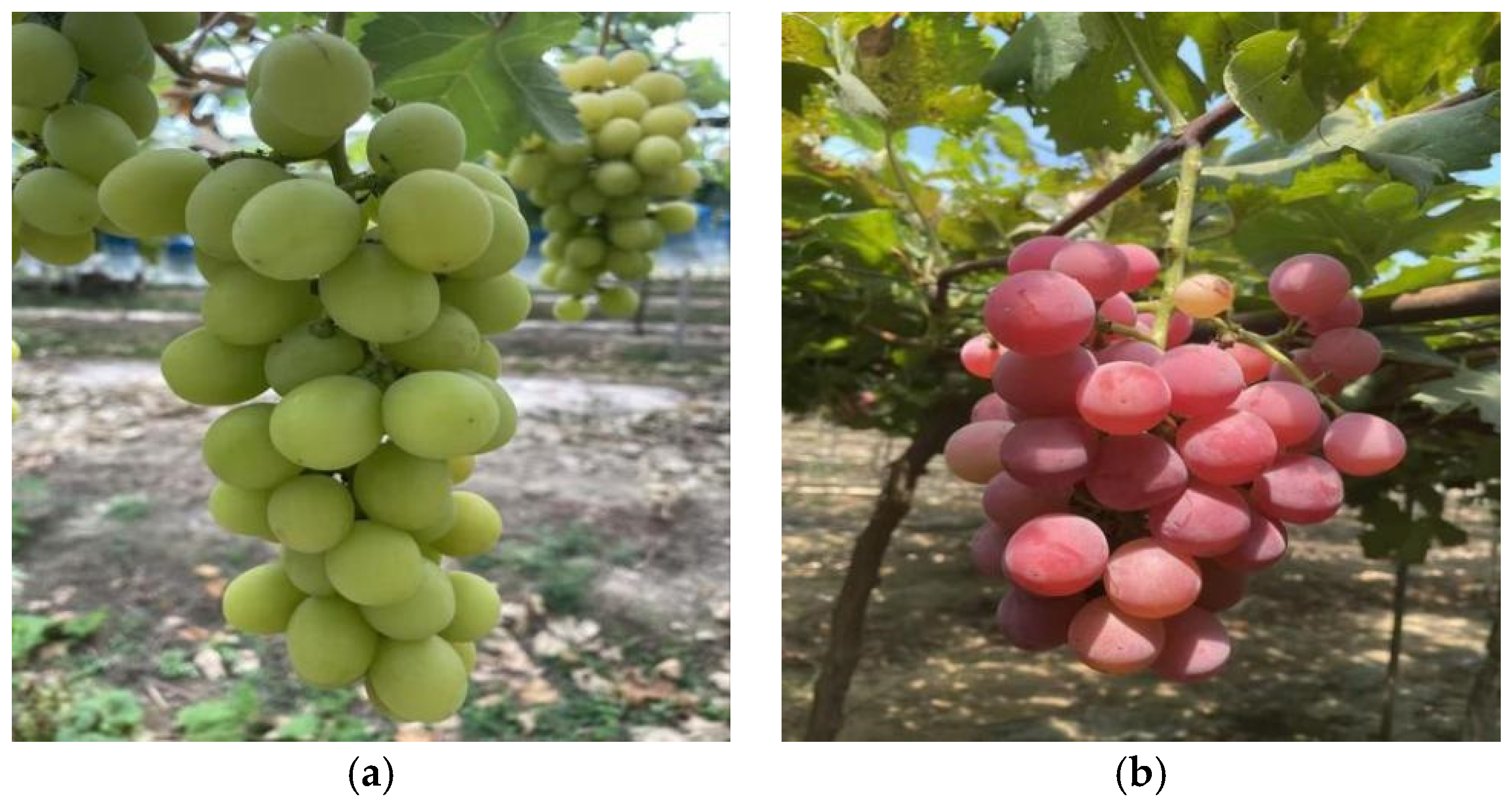
The data collection site for the present study was a specialty vineyard located in the National Modern Agricultural Demonstration Zone of Lujiang County, Hefei City, Anhui Province (31°15′33.1″ N, 117°16′58.2″ E). The region exhibits distinct seasonal climate patterns characterized by concurrent rainfall and heat events, abundant precipitation, and favorable light and thermal conditions. Photosynthesis data were collected from protected grapes (Shine Muscat and Nina Queen) planted two years prior (Figure 1). The grapevines demonstrated robust growth under artificial protected conditions, with plant rows spaced 6 m north–south and 4 m east–west.
Figure 1.
(a) Shine Muscat; (b) Nina Queen.
The experiment was carried out from 1 June to 30 September 2025, covering three key phenological stages of grapes: young fruit expansion stage (1 June to 10 July), fruit rapid expansion stage (11 July to 20 August), and fruit maturation stage (21 August to 30 September). Since daytime temperatures in summer were relatively high and plants entered a midday rest state, the collection periods were set from 9:00 to 11:30 and from 15:00 to 17:30 every sunny day.
For sample selection, healthy grape plants with consistent growth were selected, and the 6th fully expanded functional leaf from the top of the canopy was chosen as the measurement object. The selected leaves had a leaf age of about 30–35 days, with no diseases, pests or mechanical damage. This leaf position is located in the upper-middle part of the canopy, which avoids the photoinhibition of top leaves and insufficient light of lower leaves, and its photosynthetic physiological state can represent the overall level of the canopy to a certain extent [15].
The SY-1020 portable plant photosynthesis meter (Handan Chuangmeng Electronic Technology Co., Ltd., Handan, Hebei, China) was used for measurement. The instrument is equipped with an adjustable LED light source module, which can provide monochromatic light and mixed light with specific wavelengths through built-in red light (660 nm) and blue light (460 nm) LED lamp beads. Three light quality treatments were set in the present study: red light (660 nm monochromatic light), blue light (460 nm monochromatic light), and red–blue mixed light (red and blue light mixed at a photon flux ratio of 3:1).
For each light quality treatment, 10 gradient levels of photosynthetic photon flux density (PPFD) were set, which were 0, 100, 200, 400, 600, 800, 1000, 1200, 1600, and 2000 µmol m−2 s−1. It should be noted that PPFD here refers to the photon flux density in the specific waveband corresponding to each light quality; for the full photosynthetic photon flux density (400–700 nm) range, the corresponding photon flux density is the commonly referred to PPFD. During measurement, the leaf was clamped into the leaf chamber, and data recording was started after the photosynthetic rate was stable (about 2–3 min). Each sample (the same plant and the same leaf) was measured three times repeatedly under each light intensity gradient, and the average value was taken as the final measurement record [16].
The complete light response curves measured under different light qualities can not only provide full-range data support for model construction but also support the extraction of photosynthetic biochemical parameters such as maximum net photosynthetic rate (Amax), maximum carboxylation rate (Vc,max) and maximum electron transfer rate (Jmax) in subsequent physiological mechanism research. The present study focuses on the construction of a data-driven prediction model for photosynthetic rates, and the in-depth analysis of biochemical parameters will be carried out in follow-up research.
Common plant photosynthesis-related variables widely measured in physiological experiments were collected, including carbon dioxide concentration (CO2, mmol mol−1), air temperature (Ta, °C), leaf chamber temperature (T1, °C), relative humidity (RH, %), photosynthetic photon flux density (PPFD, μmol m−2 s−1), gas flow rate (J, L min−1), net photosynthetic rate (A, μmol m−2 s−1), transpiration rate (E, mmol m−2 s−1), stomatal conductance (gs, mol m−2 s−1), intercellular carbon dioxide concentration (Ci, mmol mol−1).
2.2. Data Preprocessing
2.2.1. Data Cleaning
Firstly, the full dataset was split into training, validation, and test sets using biological-replicate-level grouped stratified sampling (8:1:1). Twelve independent vine-leaf biological replicates were used: six for Shine Muscat and six for Nina Queen. The target 8:1:1 ratio describes observational measurement records instead of biological replicate numbers. Since each vine-leaf unit cannot be fragmented, whole leaves were randomly assigned at the replicate level. To maintain cultivar stratification, two replicates (one leaf of each cultivar) were allocated to the validation set, another two replicates (one leaf of each cultivar) to the test set, and the remaining eight replicates (four leaves per cultivar) to the training set. Once assigned to a subset, all measurements from a vine-leaf replicate across three phenological stages and three light-quality treatments remained entirely within that dataset, and no single leaf’s data were split across subsets. This strategy ensures each dataset includes observations covering all cultivars, phenological stages and light-quality treatments, satisfying stratification requirements at the biological replicate level. No replicate or its repeated measurements appear in multiple datasets [17]. This partitioning avoids information leakage from temporal autocorrelation of repeated leaf measurements. The validation and test sets are fully independent at the biological sample level to reliably evaluate the model’s out-of-sample generalization performance.
To comprehensively identify abnormal samples, a dual outlier detection strategy combining Z-score test and box plot algorithm was adopted [18]. All statistical thresholds for outlier judgment were calculated only based on the training set, and then directly applied to the validation and test sets to avoid data leakage.
The Z-score method judges outliers by calculating the standard deviation distance of each data point from the mean, with a threshold of |Z| > 3. The box plot method identifies outliers based on the interquartile range (IQR), with samples below Q1 − 1.5 × IQR or above Q3 + 1.5 × IQR defined as outliers. Samples meeting either of the two criteria were removed. After dual outlier detection, a total of 52 abnormal samples were removed [19].
The raw dataset contained 3150 samples for Shine Muscat and 3150 samples for Nina Queen, totaling 6300 samples; the whole dataset was then partitioned into a training set (2520 samples for each cultivar, 5040 in total), a validation set (315 samples for each cultivar, 630 in total), and a test set (315 samples for each cultivar, 630 in total).
In the present study, a total of 12 healthy grapevines (6 for Shine Muscat and 6 for Nina Queen) with consistent growth were selected as experimental plants, with 1 target functional leaf per vine, resulting in 12 independent biological replicates in total. Measurements were conducted on 35 sunny days throughout the experimental period. For each leaf, 3 light quality treatments were applied, each containing 10 light intensity gradients; each gradient was measured 3 times repeatedly, and the average value was taken as 1 independent observation record. Therefore, each leaf contributed 3 (light qualities) × 10 (light intensities) = 30 observation records per measurement session. Throughout the entire experiment, each leaf contributed approximately 525 observation records. This was combined with repeated measurements across three phenological stages to ensure growth period coverage, the total number of observations per cultivar reached 3150, and the total number of observations for the two cultivars was 6300. Specifically, each cultivar had 1050 records per phenological stage and 1050 records per light quality treatment.
2.2.2. One-Hot Encoding
Since light quality was a discrete categorical feature in the present study and cannot be directly incorporated into the numerical computations of machine learning models, using numerical codes (e.g., 1, 2, 3) to represent different light qualities may cause the model to incorrectly assume a numerical progression among them, contradicting the actual physical meaning of these features. To address this issue, dummy variable coding with red light as the reference category was employed to quantify light quality features, mapping them into binary variables; this approach eliminated interference from nonnumerical features during model training and effectively avoided multicollinearity issues caused by the dummy variable trap.
Unified coding was performed on the light quality categories of all partitioned datasets, as this coding rule only relies on the three predefined light quality categories and does not use dataset statistical information. For the categorical light quality feature, red light (660 nm) was selected as the reference category for dummy variable encoding. Blue light (460 nm) was coded as the vector [1, 0], and red–blue mixed light (photon flux ratio 3:1) was coded as [0, 1]; the reference red-light group was assigned [0, 0].
After optimized one-hot encoding, the light quality features were transformed from a single categorical column into two numerical binary columns, fully preserving the category information while avoiding numerical bias and multicollinearity issues in classification features. This enabled the light quality features to be integrated with continuous environmental variables such as carbon dioxide concentration, air temperature, and photosynthetic photon flux density during model training. The final input feature set for the BP neural network included 6 variables: 4 continuous environmental factors (photosynthetic photon flux density, carbon dioxide concentration, air temperature, relative humidity) and 2 binary variables derived from light quality one-hot encoding, corresponding to the 5 key environmental driving factors screened in the present study.
The encoded feature data were then merged with other preprocessed photosynthetic data to form a unified numerical dataset, providing a standardized input foundation for subsequent feature selection and machine learning model development.
2.2.3. Data Standardization
Lastly, min–max linear normalization was implemented after dataset partitioning. The maximum and minimum values of each feature were calculated solely from the training set. The scaling formula (1) was applied to training data, and the identical training-set-derived Xmin, Xmax parameters were directly used to transform validation and test sets, without recalculating on validation and test sets. The inverse normalization in Formula (2) also adopts the training-set extremum parameters to restore prediction results to original scale.
Linear normalization was applied to the photosynthetic feature data to standardize the scale of the data, reduce the risk of model overfitting, and accelerate model training.
This method was easy to calculate, mapped data to a specified interval, effectively preserved the relative positional relationships of data, imposed no specific requirements on data distribution, and accounted for the possibility of negative photosynthetic rates by scaling all key photosynthesis feature data to the range [0, 1]. The calculation formula is as follows:
Here, Xnorm represents the normalized data, X denotes the original data, while Xmax and Xmin represent the minimum and maximum values in the dataset, respectively.
To obtain practical photosynthetic rate values, an inverse normalization operation is required to convert the predicted results back to the original data scale. The calculation formula is as follows:
2.3. Key Feature Screening
To reduce model complexity and retain physiologically meaningful environmental drivers, we combined random forest Gini importance and maximum information coefficient (MIC) to screen key features. Combining the two indicators can comprehensively screen features from both predictive ability and statistical association, avoiding bias caused by a single metric. Random forest Gini importance measures the contribution of each feature to model prediction, while MIC captures the complex nonlinear correlation between features and the target variable [20]. The value of MIC ranges from 0 to 1, where a larger value indicates a stronger statistical association between variables, regardless of the direction of the relationship, and there is no negative value.
In the present study, MIC was calculated using the minepy library in Python, with the parameter B set to the 0.6 power of the training set sample size. The calculation was performed on the original unscaled training set data, and the pairwise MIC values were symmetric. For the categorical light quality feature, it was converted into dummy variables consistent with the model input before MIC calculation. The formula for calculating the maximum information coefficient is as follows:
In the formula, I denotes mutual information; Mc represents the maximum information coefficient, which was obtained through grid search of mutual information; and p and q indicate the number of grid cells along the horizontal and vertical axes, essentially representing the grid distribution. B was the variable, typically set to the 0.6 power of the data volume.
All calculations were performed only on the training set, and the screened key features were uniformly applied to all datasets. The specific screening results are presented in Section 3.1 of the Results section.
2.4. Improved Grey Wolf Optimization
2.4.1. Grey Wolf Optimization
The grey wolf optimization [21] simulates the predatory behavior of grey wolf packs by establishing a four-tier artificial wolf pack model that replicates their natural hunting behaviors—including tracking, encirclement, and attack—to efficiently solve complex optimization problems.
The GWO consists of three steps: establishing a social hierarchy among grey wolves, surrounding prey, and hunting prey. The detailed procedures for each step are as follows.
- (1)
- Social Hierarchy
Calculate the fitness value of each individual in the population. The three gray wolves with the highest fitness scores in the pack are labeled α, β, and δ respectively, while the remaining wolves are labeled ω.
- (2)
- Encircling Prey
The grey wolf pack demonstrates a coordinated strategy of progressive approach and encirclement toward prey through collaborative efforts [22]. The calculation formula is as follows:
In the formula, D represents the spatial distance between the grey wolf individual and the target prey, while t denotes the current iteration count of the algorithm. Xp and Xt denote the spatial coordinates of the prey and the grey wolf at iteration t, respectively, Xt+1 represents the position of the grey wolf at iteration t + 1. A and C are dynamic coefficient vectors that determine search behavior, calculated as follows:
In the formula, a represents the control parameter, whose value decreased linearly from 2 to 0, while r1 and r2 are random vectors within the interval [0, 1].
- (3)
- Hunting Prey
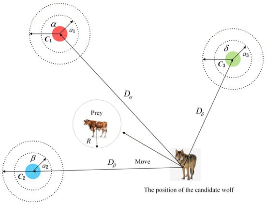
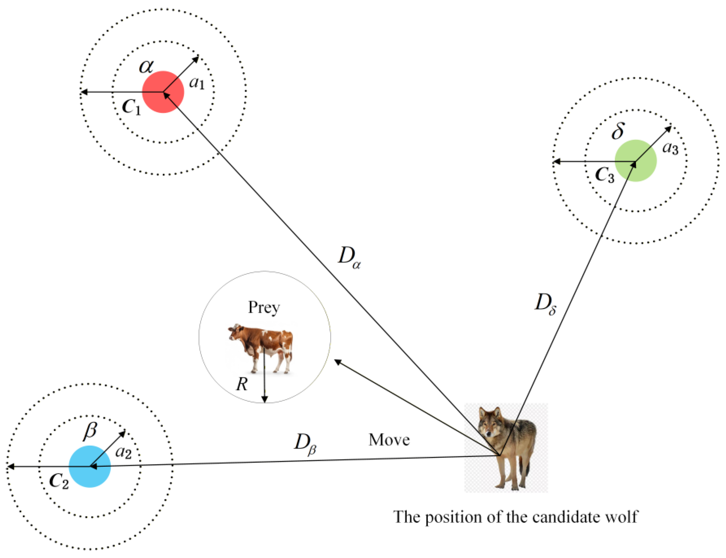
Grey wolves can perceive the approximate location of potential prey, and their search behavior primarily relies on the collaborative guidance of group members at levels α, β, and δ. To simulate the hunting strategy of grey wolves, it is assumed that some individuals in the population can effectively detect the distribution area of potential prey (the optimal solution) [23]. During the optimization process, the GWO identifies three optimal solution individuals (corresponding to levels α, β, and δ) through an elite selection mechanism; the remaining search individuals (including level ω) then perform adaptive position updates based on the coordinates of these three elite individuals. The computational formula for this collaborative search strategy is as follows:
In the formula, Dα, Dβ, and Dδ represent the distances between the current grey wolf and wolves α, β, and δ, respectively. Xα, Xβ, and Xδ denote the current position vectors of wolves α, β, and δ, while C1, C2, and C3 are random coefficient vectors. XT denotes the position vector of the ordinary grey wolf in the current iteration. The updated position of the grey wolf after iteration can be expressed as follows:
In the formula, X1, X2, and X3 represent the updated position vectors of grey wolves α, β, and δ, respectively; Xα, Xβ, and Xδ denote their position vectors at iteration t. A1, A2, and A3 are the coefficient vectors governing the position updates of wolves α, β, and δ. Dα, Dβ, and Dδ represent the distances between the current wolf and wolves α, β, and δ, respectively (Figure 2).
Figure 2.
Updated grey wolf location map.
2.4.2. IGWO Improvement Strategy
- (1)
- Tent chaotic mapping
In the GWO algorithm, the initial positions of all wolves within the population are randomly generated within the search space [24,25]. However, using random generators for population initialization often results in incomplete coverage of the solution space by search individuals. Therefore, an effective population initialization strategy must ensure uniform distribution of search individuals across all potential solution locations within the search space.
Chaotic mapping [26,27] was employed in this paper for population initialization. Chaotic sequences exhibit high randomness and ergodicity, enabling the population to explore the search space more comprehensively, effectively enhancing population diversity, preventing the algorithm from falling into local optima, and accelerating convergence to bring the search process closer to the global optimum. The Tent chaotic mapping features a relatively simple dynamic equation, is easy to implement and operate, is computationally efficient with low computational complexity, and possesses excellent distribution uniformity and strong ergodic properties [28]. The computational formula is as follows:
In the formula, Xm represents the value for the current iteration, Xm+1 is the value for the next iteration, and h is the parameter controlling the chaotic mapping behavior, which was set to 0.63 in the present study. This parameter value was selected based on existing studies on chaotic optimization, and pre-experiments verified that the Tent mapping with h = 0.63 has the best ergodicity and population uniformity in the [0, 1] interval.
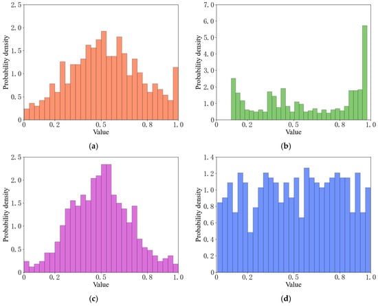
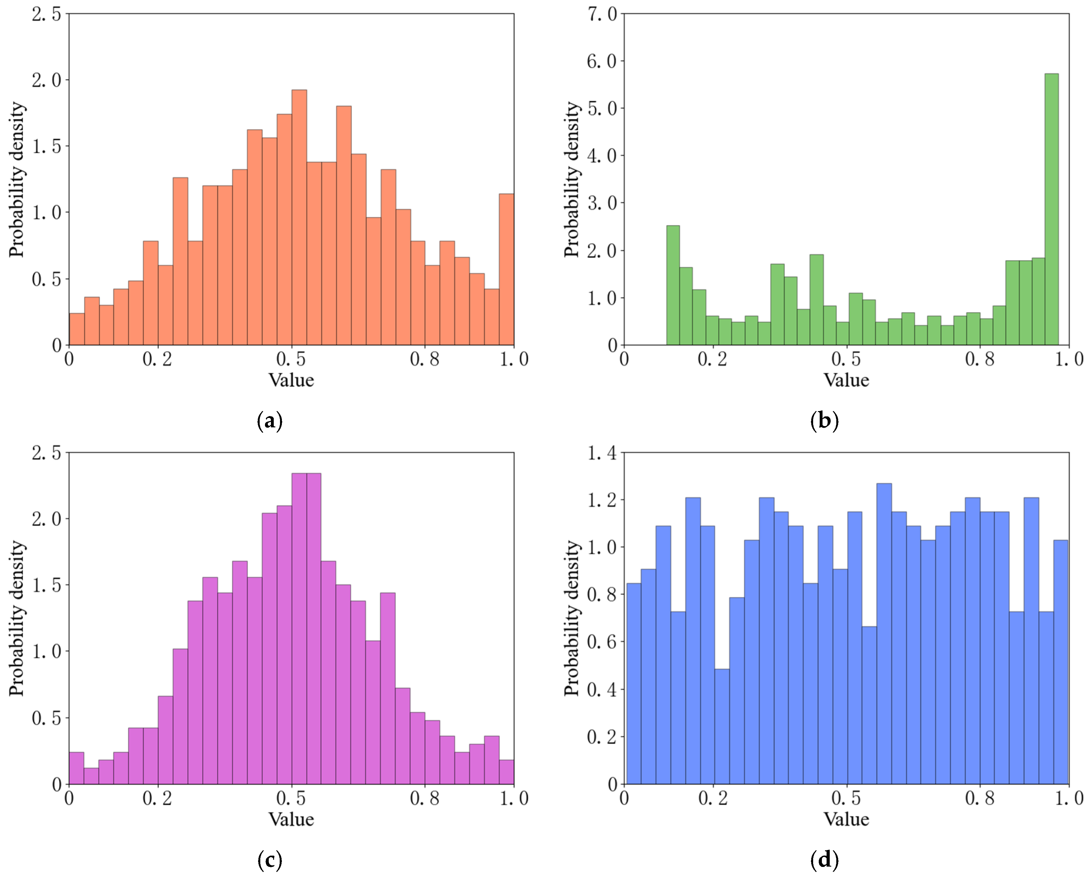
To highlight the advantages of the Tent chaotic mapping, an empirical analysis was conducted to validate its effectiveness in population initialization. Five hundred points within the interval [0, 1] were selected to initialize the grey wolf population using the random initialization method, logistic initialization method, Gaussian initialization method, and Tent initialization method, respectively. The probability density distribution of the initialization results is shown in Figure 3, where the horizontal axis represents the value of generated individuals and the vertical axis denotes probability density, reflecting the relative frequency of samples falling within each bin.
Figure 3.
Probability densities of (a) Random initialization method, (b) Logistic initialization method, (c) Gaussian initialization method, and (d) Tent initialization method.
A comparison of the random generation method, logistic chaotic mapping, Gaussian chaotic mapping, and Tent chaotic mapping demonstrated that the Tent chaotic mapping yields superior results in population initialization. Populations generated by random generation, logistic chaotic mapping, and Gaussian chaotic mapping exhibited distinct patterns of localized density and sparsity within the solution space, limiting their exploration to specific regions and resulting in suboptimal uniformity and space exploration [29]. In contrast, the Tent chaotic mapping leveraged its excellent ergodic properties and distribution features to produce a more dispersed and uniform population distribution across the entire variable range and sequence interval. This advantage enabled the population to comprehensively traverse the solution space, providing diverse and exploratory initial seeds for subsequent algorithmic searches for global optimal solutions, thereby effectively mitigating premature convergence issues.
- (2)
- Nonlinearly decreasing control parameter
In the conventional GWO algorithm, the convergence factor l serves as a critical parameter balancing global exploration and local exploitation [30,31]. To further improve optimization performance, this work introduces a nonlinear control strategy for l. With rising iteration numbers, l changes following a nonlinear rule: a large value at the early stage broadens the search range, while a small value in later iterations supports fine local searching.
In this study, a cosine function [32,33] is adopted to dynamically tune the convergence factor l. In early iterations, the designed strategy facilitates fast exploration across the whole search space and reduces the risk of stagnating in local optima. In the middle and late iterations, the algorithm shifts to refined local exploitation for accurate global optimum acquisition. The update formula of the convergence factor is expressed as follows:
In the formula, l was the convergence factor, n represented the current iteration number, m denoted the maximum number of iterations.
2.5. Model Construction and Parameter Setting
Based on the physiological mechanism that grape photosynthesis is driven by environmental factors, the present study uses the key environmental factors screened out as inputs, and takes the net photosynthetic rate as the output, to construct a BP neural network prediction model optimized by the improved GWO. The IGWO is used to optimize the initial weights and thresholds of the BP network, so as to overcome the defect that the traditional BP algorithm easily falls into local optima and improve the prediction accuracy and stability of the model.
The classical BP model parameter optimization method can yield relatively optimal parameters to some extent, but it has notable limitations [34,35,36]. In light of the key feature screening and research objectives outlined in Section 2.3, the following parameters were specified in the present study: the network adopts a single hidden layer structure, which is determined by pre-experiments and empirical formula calculation: for small and medium-sized regression tasks with 6 input dimensions, a single hidden layer with 8–15 neurons can achieve a good balance between fitting ability and generalization performance. After grid search optimization on the validation set, the number of hidden layer neurons is finally determined to be 12. An input layer with 6 neurons (corresponding to 4 continuous environmental variables and 2 one-hot encoded light quality variables), 1 hidden layer containing 12 neurons, an output layer with 1 neuron, a batch size of 128, a Sigmoid activation function, and the Adam adaptive optimization algorithm for learning rate adjustment were used. The Sigmoid activation function is selected because the normalized input and output data are all in the range of [0, 1], which matches the output range of the Sigmoid function and is conducive to the gradient propagation in the training process.
The IGWO was configured with a population size of 30, a maximum iteration count of 100, and optimization parameter bounds of [−1, 1] for BP network weights and thresholds, with MSE on the training set as the fitness function. The BP network was trained for a maximum of 100 epochs using the Adam optimizer with an initial learning rate of 0.01 and a batch size of 128. A fixed random seed of 42 was applied to all stochastic processes, including population initialization, weight initialization, and data shuffling, to ensure experiment reproducibility.
All model construction and numerical calculations in the present study were implemented in Python 3.9, in which the BP neural network was built based on PyTorch 1.12, the random forest machine learning models was implemented based on Scikit-learn 1.0, and the GWO and its improved algorithms were self-programmed. All experiments were run on a computer with an Intel(R) Core(TM) i7-9750H CPU @ 2.60GHz and 16 GB RAM.
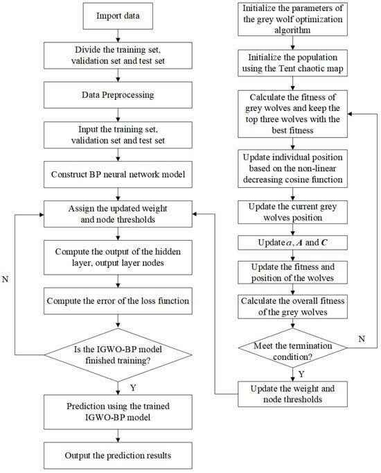
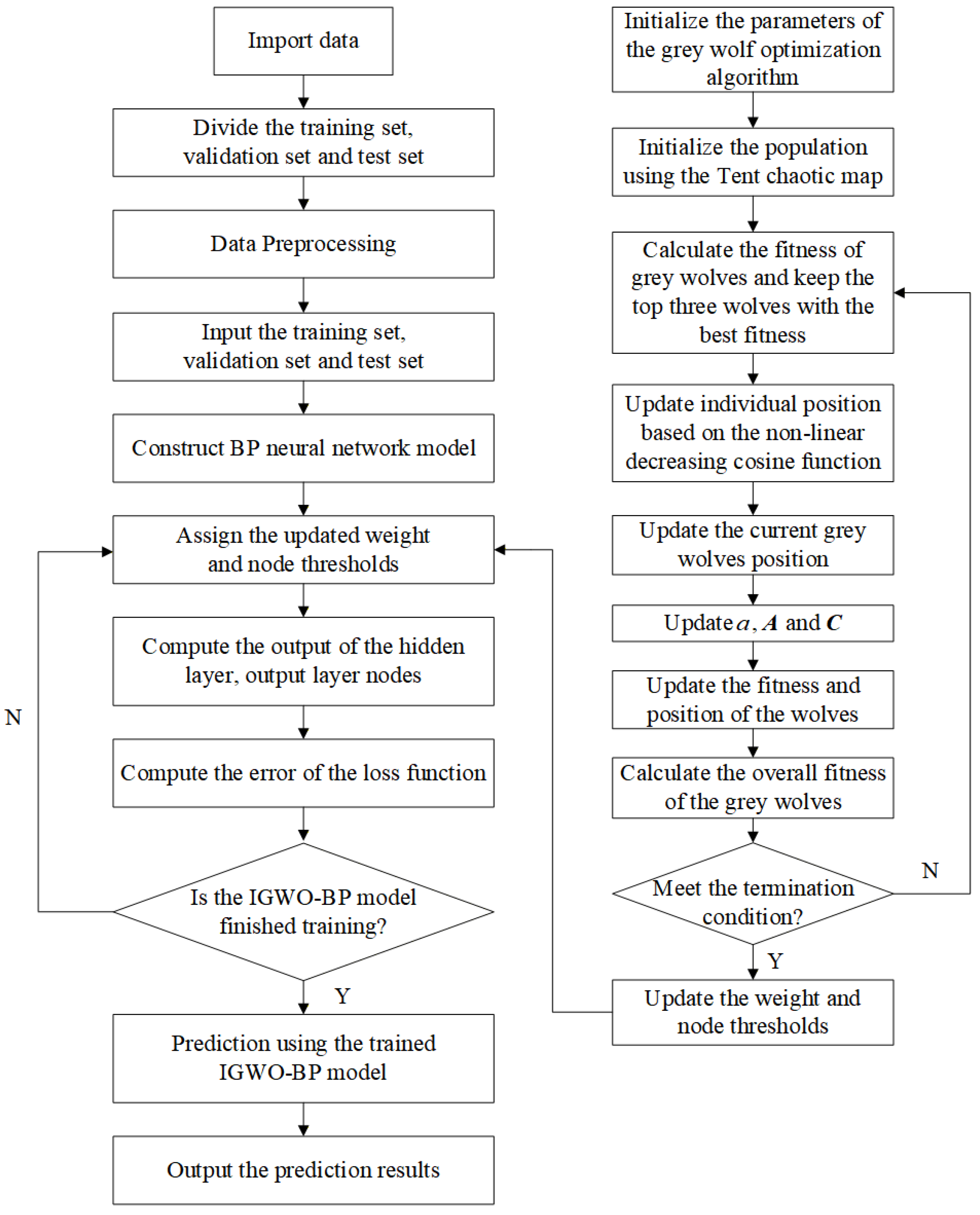
The specific implementation steps for improving the BP neural network model using the GWO are shown in Figure 4.
Figure 4.
Improved IGWO-BP prediction model workflow.
(1) After data preprocessing, import the training set, validation set, and test set containing photosynthesis data of protected grapes; (2) set the parameters of the IGWO, including population size, number of iterations, and upper/lower bounds for optimization parameters; (3) initialize population positions using the Tent chaotic mapping sequence to generate the initial population; (4) calculate the fitness values of each wolf individual in the initial population, sort them, and identify the most fit individuals as α, β, and δ; (5) update wolf positions using a nonlinear cosine function, calculate fitness scores, and sort them to obtain the next generation’s population positions; (6) calculate the fitness of each solution, compare it with the optimal value, and select the best-fitting solution as the new optimal individual [37]; (7) check whether the maximum number of iterations has been reached; terminate if so, otherwise return to step (2); (8) output the optimal parameter combination and feed it into the BP model for photosynthetic rate prediction; (9) return the predicted photosynthetic rate results.
2.6. Model Evaluation Metrics
The coefficient of determination (R2), mean square error (MSE), root mean square error (RMSE), and mean absolute error (MAE) were adopted to assess model performance. Higher R2 (near 1) and lower MSE, RMSE and MAE values represent smaller prediction errors and better model performance.
3. Results
3.1. Screening Results of Key Photosynthetic Influencing Factors
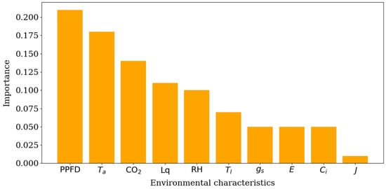
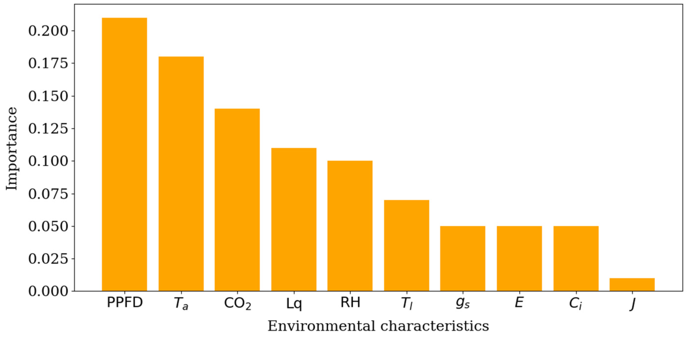
Based on the random forest Gini importance and MIC method, the Gini importance score and maximum information coefficient score of each candidate environmental feature to photosynthetic rate (A) were calculated, and the comprehensive ranking was obtained by summing the two scores. Features with a comprehensive score ≥ 0.65 were retained as model inputs.
PPFD had the highest Gini importance (0.21), followed by Ta (0.18), CO2 (0.14), Lq (0.11) and RH (0.10). The importance of other features such as E and Tl was below 0.10, and flux was the lowest (Figure 5).
Figure 5.
Random forest Gini importance of environmental characteristics for photosynthetic rate.
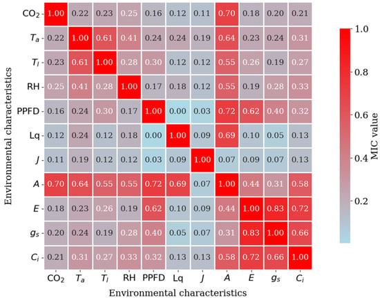
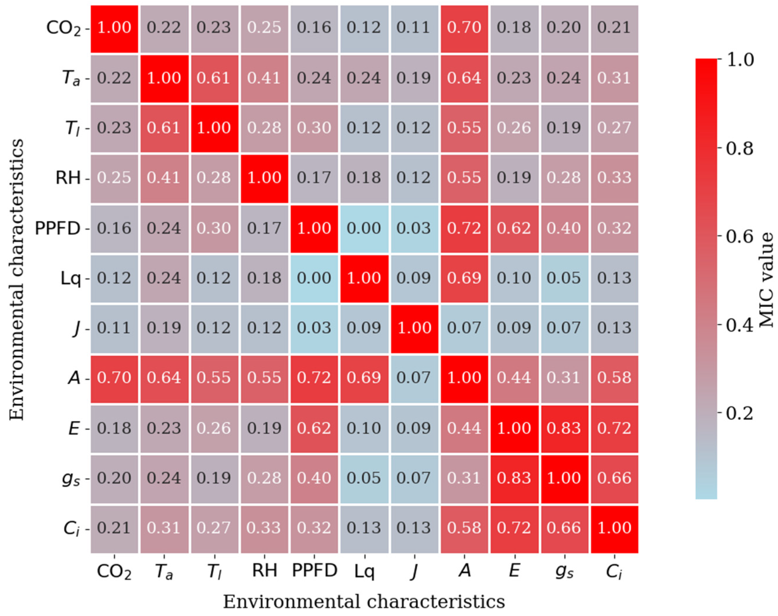
The MIC correlation analysis results are shown in Figure 6. PPFD had the strongest nonlinear correlation with A (MIC = 0.72), followed by CO2 (0.70), Lq (0.69), E (0.64), RH (0.55) and Tl (0.55). Features such as gas flow rate showed weak correlation with E.
Figure 6.
MIC heatmap of environmental characteristics and photosynthetic rate.
According to the screening threshold of comprehensive score ≥ 0.65 (to avoid overfitting and maintain model efficiency, the number of input features was limited to five. Accordingly, a threshold of 0.65 was adopted), five key environmental driving factors were finally determined: photosynthetic photon flux density, carbon dioxide concentration, air temperature, light quality and relative humidity, which were used as input variables of the prediction model.
Based on the analysis of random forest Gini importance and MIC results, and according to the combined scores in Table 1, photosynthetic photon flux density, carbon dioxide concentration, air temperature, light quality, and relative humidity were ultimately identified as the five key factors influencing photosynthetic rate.
Table 1.
Comprehensive feature importance ranking based on normalized random forest Gini importance and MIC.
3.2. Comparison of Model Performance Based on Different Optimization Algorithms
To verify the superiority of the GWO for the BP model, particle swarm optimization (PSO) [38] and the whale optimization algorithm (WOA) were employed to optimize the BP model and applied to the photosynthetic rate prediction task. Considering that all optimization algorithms and neural network training involve stochastic processes, all models were independently run 10 times, and the evaluation metrics are reported as mean ± standard deviation to reflect performance stability. Comparative experiments were conducted with the GWO-BP model, with results presented in Table 2 and Table 3.
Table 2.
Results of the validation set for the BP models using various optimization algorithms.
Table 3.
Results of the test set for the BP models using various optimization algorithms.
Table 2 and Table 3 compare the experimental prediction results of the GWO-BP model and the PSO-BP and WOA-BP models on the Shine Muscat, Nina Queen, and overall datasets, evaluated against four criteria. On the validation set, the GWO-BP model outperformed the PSO-BP model, improving R2 by 4.1%, 0.5%, and 2.1% for the Shine Muscat, Nina Queen, and overall samples, respectively; reducing MSE by 64.7%, 9.5%, and 52.9%; lowering RMSE by 40.6%, 4.8%, and 31.3%; and decreasing MAE by 42.9%, 10.2%, and 33.4%. Compared with the WOA-BP model, the GWO-BP model showed improvements of 0.5%, 0.2%, and 0.6% in R2; reductions in MSE of 19.4%, 3.9%, and 26.1%; decreases in RMSE of 19.8%, 1.9%, and 14.0%; and reductions in MAE of 9.8%, 9.4%, and 15.4%. On the test set, GWO-BP outperformed the PSO-BP model, improving R2 by 4.4%, 0.7%, and 2.0% on the Shine Muscat, Nina Queen, and overall datasets respectively; while reducing MSE by 65.3%, 11.0%, and 50.9%; RMSE by 41.1%, 5.7%, and 29.9%; and MAE by 42.0%, 8.5%, and 32.7%. Compared with the WOA-BP model, GWO-BP enhanced R2 by 0.9%, 0.7%, and 0.4%; reduced MSE by 29.6%, 11.8%, and 19.6%; decreased RMSE by 16.2%, 0.6%, and 10.4%; and lowered MAE by 8.5%, 4.4%, and 7.2%. These experimental results and analyses demonstrate that the GWO achieves more significant optimization improvements over PSO and the WOA for BP models, making it more suitable for predicting photosynthetic rates in protected grapes.
3.3. Performance Comparison of the Improved IGWO-BP Model
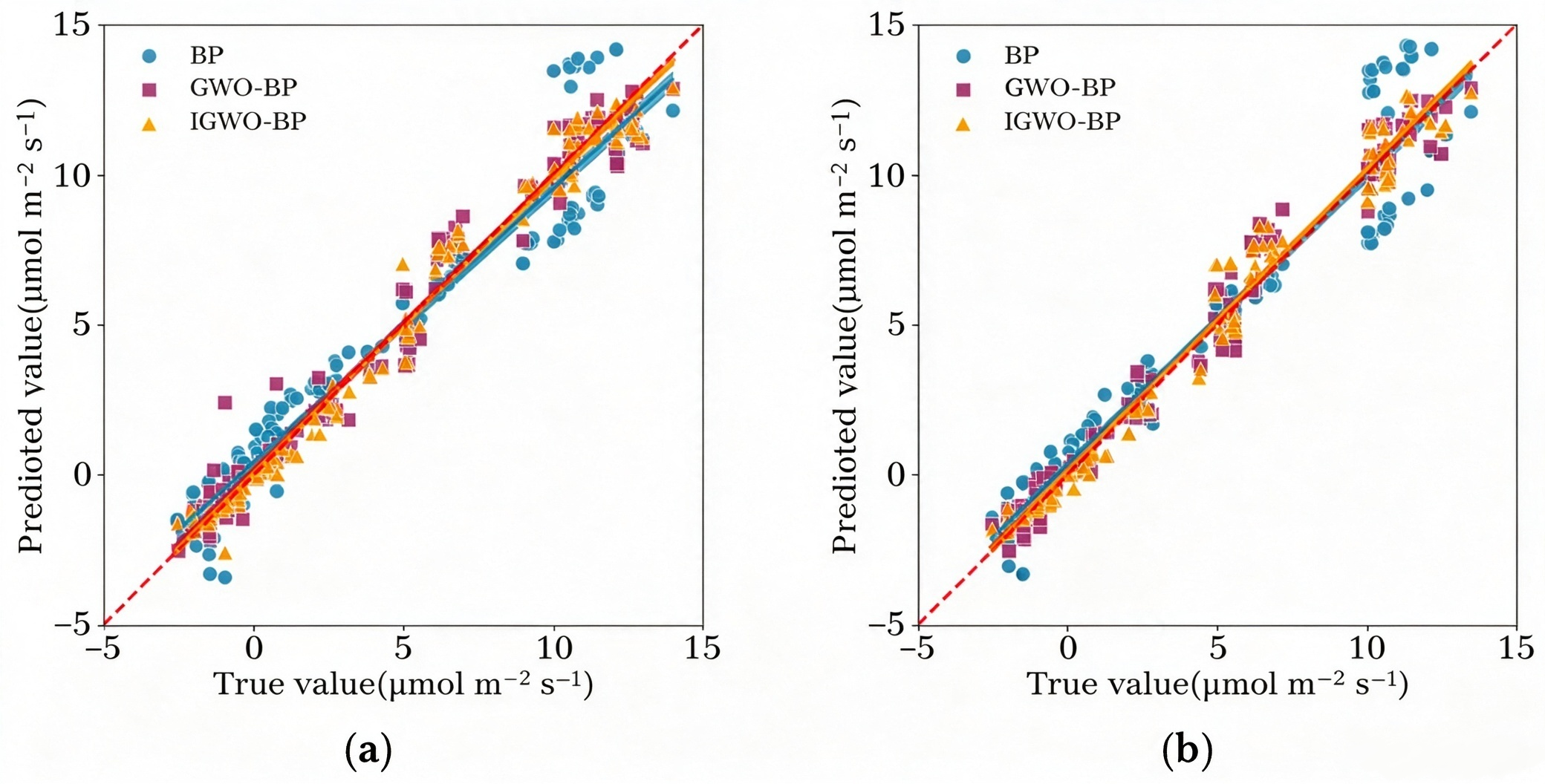
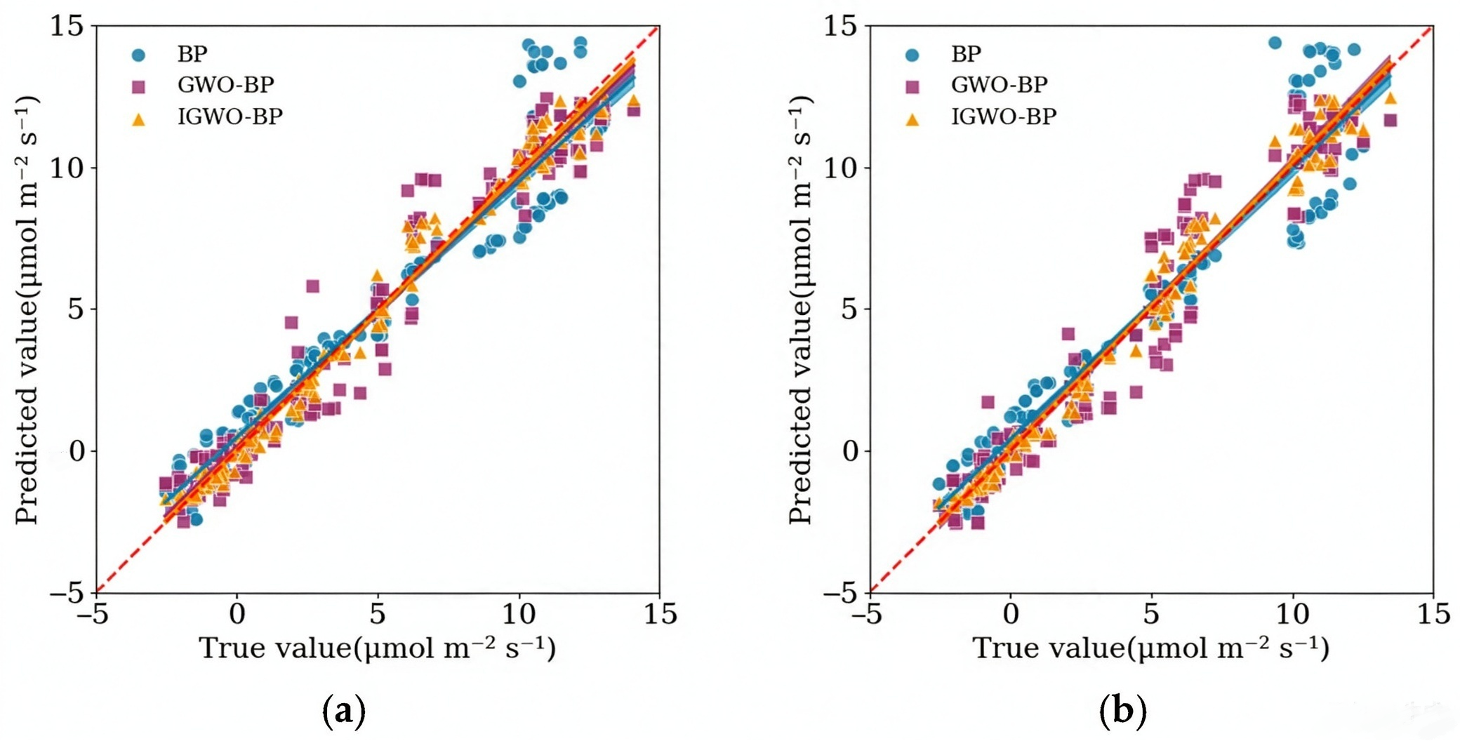
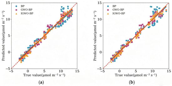
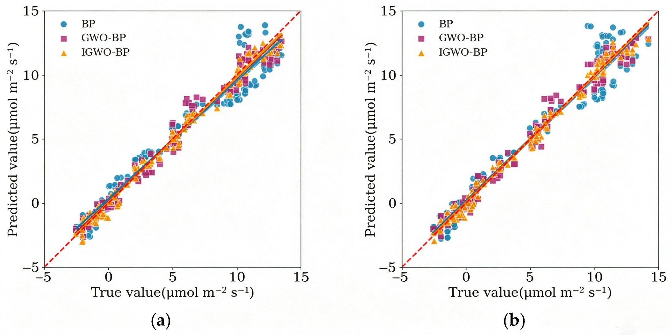
Using the segmented data from Shine Muscat, Nina Queen, and the overall sample, the IGWO-BP model was constructed for predicting photosynthetic rate in protected grapes. Specifically, samples were drawn proportionally from each subgroup of the two cultivars and three light quality treatments, with 150 representative data points selected from the validation set and test set respectively. A comparison of the prediction results among the BP, GWO-BP, and IGWO-BP models clearly demonstrates the superior performance of the IGWO-BP model. For quantitative evaluation, statistical metrics—including R2, MSE, RMSE, and MAE—were employed, accompanied by plots comparing predicted versus actual values to assess the models’ accuracy and robustness. The fitting curves of the photosynthetic rate predictions against actual values for the three models are shown in Figure 7, Figure 8 and Figure 9.
Figure 7.
(a) Shine Muscat improvement validation set results before and after; (b) Shine Muscat improvement test set results before and after.
Figure 8.
(a) Nina Queen improvement validation set results before and after; (b) Nina Queen improvement test set results before and after.
Figure 9.
(a) Total Sample improvement validation set results before and after; (b) Total Sample improvement test set results before and after.
As shown in Figure 7, Figure 8 and Figure 9, the IGWO-BP model exhibited the closest alignment between its predicted and actual photosynthetic rates, demonstrating the highest prediction accuracy. R2, MSE, RMSE, and MAE were employed as evaluation metrics to compare the predictive performance of the three models, with the comparative results presented in Table 4 and Table 5.
Table 4.
Comparison of evaluation metrics for the validation set before and after the prediction model improvement.
Table 5.
Comparison of evaluation metrics for the test set before and after the prediction model improvement.
As shown in Table 4 and Table 5, compared with the BP model and the GWO-BP model, the proposed IGWO-BP model demonstrates superior performance in predicting the photosynthetic rates of Shine Muscat and Nina Queen. Specifically, on the Shine Muscat validation set, the IGWO-BP model outperformed the BP model by increasing R2 by 5.4%, reducing MSE by 76.0%, decreasing RMSE by 51.0%, and lowering MAE by 54.0%; compared with the GWO-BP model, it improved R2 by 0.5%, reduced MSE by 24.7%, decreased RMSE by 13.3%, and lowered MAE by 14.6%. On the Shine Muscat test set, the IGWO-BP model exceeded the BP model by increasing R2 by 6.2%, reducing MSE by 74.7%, decreasing RMSE by 49.6%, and lowering MAE by 51.4%; compared with the GWO-BP model, it enhanced R2 by 0.3%, reduced MSE by 11.4%, decreased RMSE by 5.8%, and lowered MAE by 12.4%.
On the Nina Queen validation set, the IGWO-BP model outperformed the BP model by achieving a 6.4% increase in R2, a 78.2% reduction in MSE, a 53.3% decrease in RMSE, and a 53.1% reduction in MAE; compared with the GWO-BP model, it demonstrated a 3.6% improvement in R2, a 67.2% reduction in MSE, a 42.7% decrease in RMSE, and a 38.9% reduction in MAE. On the Nina Queen test set, the IGWO-BP model showed an 8.0% increase in R2, a 78.9% reduction in MSE, a 54.1% decrease in RMSE, and a 52.7% reduction in MAE compared with the BP model; relative to the GWO-BP model, it achieved a 3.6% improvement in R2, a 63.7% reduction in MSE, a 39.8% decrease in RMSE, and a 40.0% reduction in MAE.
On the overall sample validation set, the IGWO-BP model outperformed the BP model by improving R2 by 4.9%, reducing MSE by 80.0%, lowering RMSE by 55.2%, and decreasing MAE by 57.3%; compared with the GWO-BP model, it achieved an R2 improvement of 0.7%, an MSE reduction of 36.3%, an RMSE decrease of 20.1%, and an MAE reduction of 20.6%. On the overall sample test set, the IGWO-BP model showed an R2 increase of 5.0%, an MSE decrease of 81.8%, an RMSE reduction of 57.4%, and an MAE decrease of 58.0% over the BP model; relative to the GWO-BP model, it achieved an R2 improvement of 0.9%, an MSE reduction of 43.6%, an RMSE decrease of 24.9%, and an MAE reduction of 24.6%.
Collectively, these results verify that the proposed IGWO-BP model has better prediction accuracy and generalization ability for photosynthetic rate compared with the BP and GWO-BP models.
3.4. Ablation Study of Improved Strategies
To verify the contribution of each improved strategy in the IGWO, ablation experiments were conducted with four model variants: (1) GWO-BP: standard GWO optimized BP neural network. (2) Tent-GWO-BP: GWO-BP with only Tent chaotic mapping initialization strategy. (3) Nonlinear-GWO-BP: GWO-BP with only nonlinear cosine convergence factor strategy. (4) IGWO-BP: complete improved model with both Tent chaotic mapping and nonlinear cosine convergence factor. All models were tested on the total sample test set, and the results are shown in Table 6.
Table 6.
Ablation study results on total sample test set.
The ablation results show that both improved strategies contribute to the performance improvement of the model. Compared with the baseline GWO-BP model, the Tent-GWO-BP model with only chaotic initialization reduces MAE by 9.9%, and the Nonlinear-GWO-BP model with only nonlinear convergence factor reduces MAE by 15.1%. The complete IGWO-BP model integrating both strategies achieves the best performance, with MAE reduced by 24.6%, indicating that the two improved strategies have a synergistic effect. The Tent chaotic mapping enhances population diversity and avoids premature convergence, while the nonlinear cosine convergence factor balances global and local search capabilities, and their combination further improves the prediction accuracy and stability of the model.
4. Discussion
The principal novelty of this study is twofold. First, light quality was introduced as an input factor into a protected grape photosynthetic rate prediction model alongside four conventional environmental drivers, which compensates for the neglect of spectral regulatory effects in previous models. Second, an improved grey wolf optimization algorithm, integrating Tent chaotic mapping and a nonlinear decreasing cosine convergence factor, was developed to overcome the premature convergence of the standard GWO. In addition, the model was validated with a biological-replicate-level independent data splitting strategy, which avoids information leakage and provides a more objective assessment of out-of-sample generalization.
The feature screening results support Hypothesis 1 that incorporating light quality as an input factor can effectively improve the prediction accuracy of the photosynthetic rate model. Light quality ranked fourth (combined importance score of 0.80) among the ten candidate features, ahead of relative humidity and clearly above transpiration rate and leaf chamber temperature, indicating that it conveys information that conventional environmental factors do not fully capture. This finding addresses the factor gap in previous protected crop photosynthetic rate models, whose inputs were restricted to temperature, humidity, photosynthetic photon flux density and CO2 and did not consider light quality [5,6]. The results imply that omitting light quality may discard a meaningful part of the environmental information regulating grape photosynthesis and that the spectral composition of light should be included when constructing data-driven prediction models for protected cultivation.
Regarding Hypothesis 2, the comparison experiments confirm that the improved optimization strategy alleviates premature convergence and enhances prediction performance. On the overall sample test set, the IGWO-BP model achieved an R2 of 0.990, exceeding the conventional BP (0.943), GWO-BP (0.981) and the PSO-BP and WOA-BP variants. The ablation study further demonstrated that each improvement acts independently: Tent chaotic initialization reduced MAE by 9.9%, the nonlinear cosine convergence factor reduced MAE by 15.1%, and their combination reduced MAE by 24.6% relative to GWO-BP, confirming a synergistic effect. These results are consistent with previous applications of chaotic mapping and adaptive convergence-factor strategies to strengthen GWO in agricultural optimization [10,11,13] and show that enhancing population initialization and the convergence-factor mechanism is an effective way to improve the prediction accuracy and stability of BP-based models for complex physiological data.
From a physiological perspective, the ranking of the selected factors is consistent with the classical mechanism of photosynthesis. Photosynthetic photon flux density, as the energy source of the light reaction, ranked first; CO2, as the substrate of carbon assimilation, ranked second; air temperature and light quality regulate enzymatic activity and the distribution of light energy between the two photosystems; and relative humidity acts indirectly through stomatal conductance [1,20]. The consistency of this ranking between the two cultivars indicates that the environmental driving mechanism of grape photosynthesis is largely universal across cultivars, supporting the generalizability of the proposed input system.
Nevertheless, several limitations should be acknowledged. The model was developed using data from only two grape cultivars, a single experimental site and a single growing season, so its extrapolation to other regions, cultivars and climatic conditions remains to be verified. In addition, the present study focused on a data-driven prediction approach and did not extract biochemical parameters (e.g., Amax, Vc,max and Jmax) from the light–response curves; incorporating such mechanistic parameters may further improve accuracy and interpretability. Multi-site, multi-cultivar and cross-season experiments are therefore required to consolidate the generalization ability of the model and to support its application in intelligent protected environmental control.
5. Conclusions
This study tested two research hypotheses: (1) incorporating light quality as an input variable can effectively improve the prediction accuracy of the grape photosynthetic rate model; (2) modifying the population initialization strategy and convergence factor adjustment mechanism of GWO can mitigate premature convergence and enhance model prediction performance. Both hypotheses were supported by the present results. Using random forest Gini importance and MIC analysis, five key environmental factors including light quality were screened, and their importance ranking was consistent with grape photosynthetic physiology and showed good universality across the two tested cultivars. The proposed IGWO-BP model outperformed BP, PSO-BP and GWO-BP benchmark models for both cultivars and pooled samples, capturing the complex nonlinear relationship between environmental factors and photosynthetic rate. This model can provide theoretical basis and data support for intelligent environmental control systems and dynamic regulation of light, temperature, humidity and CO2 concentration in protected grape cultivation to support high-quality and high-yield protected agriculture production. It should be noted that the model was built using experimental data of two grape cultivars collected from a single site within one growing season in Hefei; its generalization across other regions, cultivars and seasons still requires further validation, and future work will carry out multi-site, multi-cultivar and cross-season experiments to improve the generalization ability of the model.
Author Contributions
Conceptualization, F.Y. and H.L.; methodology, F.Y., H.L. and M.L.; validation, F.Y., Z.M. and X.L.; formal analysis, F.Y., M.X. and M.L.; investigation, F.Y. and M.X.; resources, H.L., M.X. and Q.Z.; data curation, F.Y. and X.L.; writing—original draft preparation, F.Y.; writing—review and editing, H.L., M.X. and Q.Z.; visualization, F.Y. and Z.M.; supervision, M.L. and Q.Z.; project administration, H.L. and M.X.; funding acquisition, H.L. and M.X. All authors have read and agreed to the published version of the manuscript.
Funding
This research was funded by the Anhui Provincial Key Research and Development Program, grant number 2023n06020027; the 2025 Anhui Provincial University Outstanding Young Teachers Cultivation Program, grant number YQYB2025101; and the China National Key Research and Development Program, grant number 2022YFD2002104.
Data Availability Statement
The original contributions presented in the present study are included in this article. Further inquiries can be directed to the corresponding author.
Conflicts of Interest
The authors declare no conflicts of interest.
References
- Wilcox, J.; Fettkether, L.; Wright, J. Making plants matter: Modeling photosynthesis. Sci. Teach. 2025, 92, 26–37. [Google Scholar] [CrossRef] [Scilit]
- Li, Y.; Ding, Y.; Li, D.; Miao, Z. Automatic carbon dioxide enrichment strategies in the greenhouse: A review. Biosyst. Eng. 2018, 171, 101–119. [Google Scholar] [CrossRef] [Scilit]
- Yang, J.; He, J.; Liu, F.; Cu, X. Research progress on effects of different soil moisture on plant photosynthesis. Water Sav. Irrig. 2023, 11, 39–46. [Google Scholar] [CrossRef]
- Pu, L.; Li, Y.; Gao, P.; Zhang, H.; Hu, J. A photosynthetic rate prediction model using improved RBF neural network. Sci. Rep. 2022, 12, 9563. [Google Scholar] [CrossRef] [Scilit] [PubMed]
- Song, H.; Zhao, X.; Liu, P. LI-RBF algorithm based for prediction model research in the application of photosynthetic rate. Comput. Meas. Control 2013, 21, 2641–2644. [Google Scholar]
- Li, T.; Ji, Y.; Zhang, M.; Sha, S.; Jiang, Y. Tomato photosynthetic rate prediction models under interaction of CO2 enrichments and soil moistures. Trans. Chin. Soc. Agric. Mach. 2015, 46, 208–214. [Google Scholar] [CrossRef]
- Tao, Y. Research on Prediction Model of Cucumber Photosynthesis Based on BP Neural Network. Master’s Thesis, Northwest A&F University, Yangling, China, 2016. [Google Scholar]
- Miao, Y.; Liu, L.; Wang, M.; Zeng, Z.; Zhang, J.; Cheng, Y.; Li, B. A photosynthetic rate prediction model for cucumber based on a machine learning algorithm and multi-factor environmental analysis. Horticulturae 2025, 11, 1475. [Google Scholar] [CrossRef] [Scilit]
- Ji, H.; He, X.; Wang, W.; Zhang, H. Prediction of winter wheat harvest based on back propagation neural network algorithm and multiple remote sensing indices. Processes 2023, 11, 293. [Google Scholar] [CrossRef] [Scilit]
- Piri, J.; Kahkhamoghadam, P.; Chari, M.M. A comparison of quantum-inspired GMDH-HS and GMDH-GWO approaches to soil hydraulic conductivity prediction. J. Hydrol. Reg. Stud. 2025, 61, 102627. [Google Scholar] [CrossRef] [Scilit]
- Morán-Figueroa, G.H.; Cobos-Lozada, C.A.; Bedoya-Leyva, O.F. Optimizing agricultural management practices for maize crops: Integrating clusterwise linear regression with an adaptation of the grey wolf optimizer. Agriculture 2025, 15, 2068. [Google Scholar] [CrossRef] [Scilit]
- Wu, L.; Tian, J.; Liu, Y.; Wang, Y.; Zhang, P. Multi-objective planting structure optimisation in an irrigation area using a grey wolf optimisation algorithm. Water 2024, 16, 2297. [Google Scholar] [CrossRef] [Scilit]
- Xu, X.; Xu, Y.; Zhou, Y.; Li, R.; Wang, Y.; Lian, H.; Chen, Y.; Zhang, Z.; Li, M. An intelligent and uncertain optimization framework for water-nitrogen synergistic management under extreme supply and demand water risks. Expert Syst. Appl. 2025, 282, 127829. [Google Scholar] [CrossRef] [Scilit]
- Ahmed, A.A.M.; Sharma, E.; Jui, S.J.J.; Deo, R.C.; Nguyen-Huy, T.; Ali, M. Kernel ridge regression hybrid method for wheat yield prediction with satellite-derived predictors. Remote Sens. 2022, 14, 1136. [Google Scholar] [CrossRef] [Scilit]
- Somkuwar, R.; Dhole, A. Understanding the photosynthesis in relation to climate change in grapevines. Theory Biosci. 2025, 144, 107–120. [Google Scholar] [CrossRef] [Scilit] [PubMed]
- Cui, D. Research on Digitization of Shine Muscat Grape Production. Master’s Thesis, Shandong Agricultural University, Tai’an, China, 2022. [Google Scholar]
- Filipovics, M.; Komasilova, O.; Bimsteine, G.; Zacepins, A.; Zagorska, V.; Komasilovs, V. Characterization of disease-specific spectra in tomato early blight using hyperspectral image analysis. Agriculture 2026, 16, 2138. [Google Scholar] [CrossRef] [Scilit]
- Wang, R.; Feng, J.; Zhang, W.; Liu, B.; Wang, T.; Zhang, C.; Xu, S.; Zhang, L.; Zuo, G.; Lv, Y.; et al. Detection and correction of abnormal IoT data from tea plantations based on deep learning. Agriculture 2023, 13, 480. [Google Scholar] [CrossRef] [Scilit]
- Lopin, P.; Nawsang, P.; Laywisadkul, S.; Lopin, K.V. Evaluation of Low-Cost Multi-Spectral Sensors for Measuring Chlorophyll Levels Across Diverse Leaf Types. Sensors 2025, 25, 2198. [Google Scholar] [CrossRef] [Scilit] [PubMed]
- Zhang, H.; Zhang, Z.; Zhang, S.; Hu, J.; Xin, P.; Wang, Z. Analysis of main influencing factors and modeling of photosynthetic rate for cucumber at initial flowering stage. Trans. Chin. Soc. Agric. Mach. 2017, 48, 242–248. [Google Scholar] [CrossRef]
- Zhang, Y.; Guo, B.; Wang, Q.; Fan, Y. Prediction of water consumption in Binzhou based on IGWO-BP model. China Rural Water Hydropower 2025, 6, 95–101. [Google Scholar] [CrossRef]
- Gao, F. Multi-objective distribution path optimization of cold chain logistics based on improved grey wolf optimizer. Discov. Comput. 2026, 29, 276. [Google Scholar] [CrossRef] [Scilit]
- Zhang, Y.; Qiu, J.; Zhang, Y.; Xie, Y. The adoption of a support vector machine optimized by GWO to the prediction of soil liquefaction. Environ. Earth Sci. 2021, 80, 360. [Google Scholar] [CrossRef] [Scilit]
- Lang, X.; Li, P.; Zhang, B.; Cao, J.; Guo, Y.; Kan, Z.; Lu, S. Localization of multiple leaks in a fluid pipeline based on ultrasound velocity and improved GWO. Process Saf. Environ. Prot. 2020, 137, 1–7. [Google Scholar] [CrossRef] [Scilit]
- Fatemeh, B.; Saeed, S.; Saleh, H.J. A new insight into metaheuristic optimization method using a hybrid of PSO, GSA, and GWO. Structures 2022, 44, 1168–1189. [Google Scholar] [CrossRef] [Scilit]
- Kohli, M.; Arora, S. Chaotic grey wolf optimization algorithm for constrained optimization problems. J. Comput. Des. Eng. 2018, 5, 458–472. [Google Scholar] [CrossRef] [Scilit]
- Li, Y.; Lin, X.; Liu, J. An improved gray wolf optimization algorithm to solve engineering problems. Sustainability 2021, 13, 3208. [Google Scholar] [CrossRef] [Scilit]
- Dong, Y.; Zhang, Z.; Hong, W.-C. A hybrid seasonal mechanism with a chaotic cuckoo search algorithm with a support vector regression model for electric load forecasting. Energies 2018, 11, 1009. [Google Scholar] [CrossRef] [Scilit]
- Liu, S.; Wang, X.; Peng, J. Construction of comprehensive energy system evaluation model for industrial parks combining IGWO and SVM. Acta Energ. Sol. Sin. 2026, 47, 74–81. [Google Scholar] [CrossRef]
- Jiang, Z.; Li, C.; Yang, X.; Li, X.; Liu, X.; Mo, J.; Han, L. Survey of grey wolf optimization algorithm. Comput. Eng. Appl. 2025, 61, 76–105. [Google Scholar]
- Yang, S.; Gong, Y.; Wang, W. Active disturbance rejection control of air conditioning supply air temperature based on improved gray wolf algorithm. Sci. Technol. Eng. 2025, 25, 5491–5500. [Google Scholar]
- Padhy, S.; Panda, S.; Mahapatra, S. A modified GWO technique based cascade PI-PD controller for AGC of power systems in presence of plug-in electric vehicles. Eng. Sci. Technol. Int. J. 2017, 20, 427–442. [Google Scholar] [CrossRef] [Scilit]
- Liu, L.-W.; Hsieh, S.-H.; Lin, S.-J.; Wang, Y.-M.; Lin, W.-S. Rice blast (magnaporthe oryzae) occurrence prediction and the key factor sensitivity analysis by machine learning. Agronomy 2021, 11, 771. [Google Scholar] [CrossRef] [Scilit]
- Garai, S.; Paul, R.K.; Rakshit, D.; Yeasin, M.; Emam, W.; Tashkandy, Y.; Chesneau, C. Wavelets in combination with stochastic and machine learning models to predict agricultural prices. Mathematics 2023, 11, 2896. [Google Scholar] [CrossRef] [Scilit]
- Yu, L.; Xie, L.; Liu, C.; Yu, S.; Guo, Y.; Yang, K. Optimization of BP neural network model by chaotic krill herd algorithm. Alex. Eng. J. 2022, 61, 9769–9777. [Google Scholar] [CrossRef] [Scilit]
- Panda, S.; Panda, G. Performance evaluation of a new BP algorithm for a modified artificial neural network. Neural Process. Lett. 2020, 51, 1869–1889. [Google Scholar] [CrossRef] [Scilit]
- Zhang, X.; Xu, R.; Feng, X.; Ye, L. Differential evolution GWO optimized RBFNN and its grain yield prediction application. Comput. Eng. Des. 2024, 45, 3802–3811. [Google Scholar]
- Yu, F.; Wang, X.; Liu, J.; Huang, J.; Tan, W.; Ma, B.; Niu, H. Network model prediction of spring flow in the Xiaonanhai spring basin based on PSO-BP neural network model. Geol. Explor. 2025, 61, 1314–1323. [Google Scholar]

Disclaimer/Publisher’s Note: The statements, opinions and data contained in all publications are solely those of the individual author(s) and contributor(s) and not of MDPI and/or the editor(s). MDPI and/or the editor(s) disclaim responsibility for any injury to people or property resulting from any ideas, methods, instructions or products referred to in the content. |
© 2026 by the authors. Licensee MDPI, Basel, Switzerland. This article is an open access article distributed under the terms and conditions of the Creative Commons Attribution (CC BY) license.