Monocular Metric-Depth Adaptation for Agricultural Perception: A CitrusFarm Case Study with Embedded Inference

Abstract

Adapting monocular metric depth to agricultural imagery requires balancing target-domain accuracy against the scope of model updates and embedded execution cost. We evaluate SARE-Depth on CitrusFarm using a frozen teacher-guided Depth Anything V2 Small base. Depth-Preserving Residual Head Refinement (DP-RHR) learns image-level log-scale and gated local corrections, followed by fixed depth-conditioned Range-Expert (RE) refinement. Before adaptation, fixed-checkpoint evaluations show persistent overestimation under both square and aspect-preserving input. On 750 internal-test images with common FP32 references and a 30 m cap, scalar calibration reduces absolute relative error (AbsRel) from 4.782 to 0.476. DP-RHR reaches 0.325 with 93,123 updated parameters; complete metric-head fine-tuning achieves 0.220 ± 0.006 across three runs with 2,728,513 updated parameters. Subsequent RE refinement provides smaller, domain-dependent gains with reduced threshold accuracy, while separate Dingxi examples reveal object-distance underestimation. Cumulative Jetson Orin NX latency increases from 26.87 ms for the base to 31.49 ms with DP-RHR and 35.08 ms for the complete path. These comparisons relate adaptation scope to accuracy and measured execution cost in this agricultural case study.

1. Introduction

Agricultural machinery uses scene geometry to navigate, approach targets and judge working distances [1,2]. Vision-based guidance and harvesting therefore require spatial information alongside target recognition [3,4,5]. Fruit detection and crop-weed segmentation identify objects and operational regions [6,7], while depth-camera crop-row mapping and paired colour-depth datasets illustrate the complementary role of geometry [8,9].

Monocular depth addresses three practical settings: machinery equipped only with a single RGB camera, retrofits retaining an existing camera, and fallback operation when stereo correspondence becomes unreliable. These settings motivate estimating distance from the available image stream for target approach and anticipation of row endings. Their sensing requirements connect depth error with the time available for an operational response.

Agricultural depth estimation has been studied through different supervision and adaptation routes. MonoDA trains lightweight depth and pose networks on KITTI sequences by self-supervised view reconstruction and evaluates vineyard imagery and Jetson TX2 inference [10]. Divyanth et al. use a modified Pix2Pix network with apple-orchard imagery from two cultivation systems and different cameras [11]. AgriLoRA-DA combines low-rank attention-projection updates in a frozen Depth Anything V2 encoder with a Lite-FPNHead decoder; its supervised WE3DS evaluation includes median scale alignment [12]. These studies motivate adaptation to agricultural imagery, while leaving open the accuracy and computational consequences of correcting a compact metric predictor without updating its existing depth path.

General depth methods supply transferable representations through multiscale prediction, residual networks, ordinal regression and image-reconstruction supervision [13,14,15,16,17]. Scale- and shift-invariant learning enables training across heterogeneous datasets [18], and dense prediction transformers combine global features with multiscale decoding [19]. Depth Anything and Depth Anything V2 extend this approach through large-scale unlabelled imagery and teacher-generated targets [20,21]. Recovering distances in metres additionally involves scale and camera modelling: adaptive depth bins and metric heads [22,23], canonical-camera normalization [24,25], metric prediction without inference-time camera metadata [26], and camera-general formulations [27,28]. Diffusion-based affine-invariant prediction [29] and language-conditioned scale-shift conversion [30] address related depth representations. The present study starts with an already metric predictor and examines supervised correction on orchard data.

Compact base preparation and agricultural adaptation have distinct roles. Knowledge distillation transfers teacher information to a student [31,32], with intermediate-feature and attention supervision providing other transfer mechanisms [33,34]. Efficient convolutional architectures and compact depth networks address embedded execution [35,36]. Here, dataset reference depths and offline Depth Pro targets jointly train a Depth Anything V2 Small student, whose depth path is subsequently frozen. Parameter efficiency refers to the number of parameters updated during target-domain adaptation; inference cost is measured independently.

The location of those updates is a substantive design choice. Residual adapters, low-rank updates and lightweight transformer modules provide alternatives for adapting shared representations [37,38,39]. We instead learn output corrections from base depth and frozen decoder features. A single training-fitted scale tests how much error can be removed by calibration alone, whereas fine-tuning the complete original metric-depth head measures the gain from updating a larger portion of the predictor. These controls place output-side adaptation between scalar calibration and decoder adaptation under shared target-domain data and evaluation conditions.

We ask two questions: how does joint global-scale and local-residual adaptation compare with scalar calibration and complete metric-head fine-tuning, and what does depth-conditioned residual refinement add beyond output clipping or a single residual head? Fixed-checkpoint preprocessing tests first characterize the base scale bias. The adaptation and refinement comparisons then separate changes in accuracy from updated-parameter count and measured execution cost.

SARE-Depth (Scale Adaptation and Range Experts) addresses these questions in stages. Depth-Preserving Residual Head Refinement (DP-RHR) learns an image-level log-scale adjustment and a gated local residual from the frozen base. Its output becomes a frozen anchor for Range-Expert (RE) refinement. Four feature-based residual predictions are combined using anchor-depth-dependent weights, and their mixture is bounded before log-depth fusion. In contrast to learned expert allocation [40,41], the routing centres and temperature are fixed while the weights vary with pixel depth.

The study evaluates this design against scalar calibration, complete metric-head fine-tuning and two near-parameter-matched residual heads. CitrusFarm provides the principal dense evaluation, complemented by domain-specific comparisons, recording-group partitions, separate-location Dingxi object-distance measurements and embedded execution tests. The resulting evidence relates the scope of adaptation to its accuracy, data dependence and computational cost.

2. Materials and Methods

2.1. Framework Overview

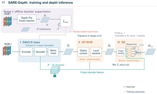
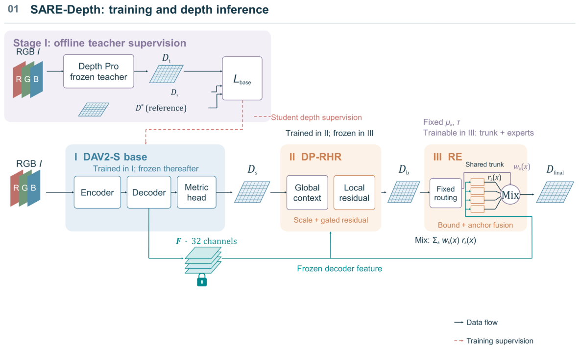
Figure 1 summarizes the SARE-Depth framework. Stage I establishes a compact teacher-guided metric-depth base. Stage II adapts the frozen base through global-scale and local-residual correction, and Stage III applies range-expert refinement to the resulting frozen anchor.

Figure 1. Training scopes and depth-inference path of SARE-Depth.

An RGB input I has size 3 × H × W, where H and W denote image height and width. D_s denotes the student depth output during base training and after freezing. All depth predictions are in metres. D* denotes dataset reference depth, and D_t denotes offline teacher targets.

Stage I: Teacher-guided metric-depth base. Dataset references and offline Depth Pro targets supervise the DAV2-S encoder, decoder and metric-depth head. After training, the frozen model provides depth D_s and the final 32-channel decoder feature F to both correction stages. Section 2.3 defines the supervised and distillation objectives.

Stage II: Global-scale and local-residual adaptation. DP-RHR predicts an image-level log-scale adjustment and a gated, bounded local residual from D_s and F. Joint target-domain training produces the depth anchor D_b. The base remains frozen during adaptation, and DP-RHR is frozen after checkpoint selection.

Stage III: Range-expert refinement. RE uses D_b to compute routing weights and F to predict four residual fields. Fixed centres are estimated from training-anchor predictions. The weighted residual mixture is bounded and applied in log-depth space to produce D_final. Only the shared RE trunk and expert heads are updated.

SARE-Depth denotes the complete base + DP-RHR + RE depth-inference pipeline. KITTI and NYUv2 share one DP-RHR anchor trained jointly on their public training data, whereas CitrusFarm uses a separately trained agricultural anchor. Each domain has its own RE parameters and fixed routing centres estimated from the corresponding training-anchor predictions. Table 1 summarizes the inputs, trainable and frozen components, outputs, and objectives of the three depth stages.

Table 1. Inputs, outputs, and optimization scope of the three depth stages.

Stage	Data Inputs	Updated	Frozen	Output	Objective
I	RGB I; dataset D*; teacher Dt	DAV2-S depth path	Depth Pro teacher	Ds; F	SILog + log-depth KD
II	Base depth Ds; final feature F; dataset D*	DP-RHR	Base	Anchor Db	Log + metric error; bounded-correction penalties
III	Anchor Db; feature F; dataset D*	RE trunk and heads	Base; DP-RHR; fixed routing	Dfinal	Log + metric error; preservation, gradient, residual terms

Note: The stages describe the depth path. Its parameter inventory is reported in Section 3.2.

Detailed network operations and optimization objectives are introduced in Section 2.3, Section 2.4 and Section 2.5.

2.2. Datasets and Evaluation Splits

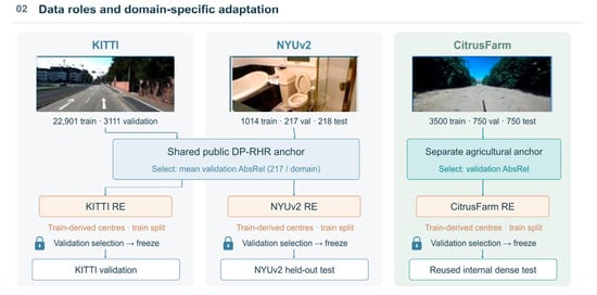
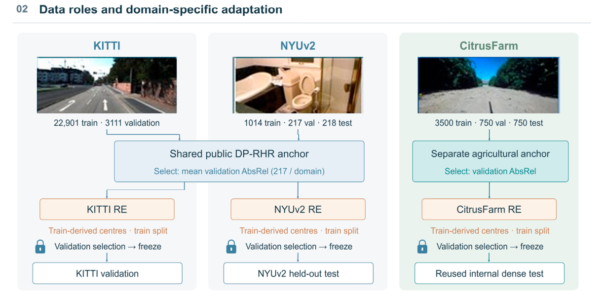
Figure 2 summarizes how each data source is used for training, model selection, or post-selection evaluation.

Figure 2. Data roles and domain-specific adaptation.

KITTI supplies driving images with projected lidar reference depth [42], with 22,901 training and 3111 validation pairs from 62 and 10 scenes. NYUv2 supplies indoor RGB-D data [43], partitioned into 1014 training, 217 validation and 218 held-out test images. The prepared CitrusFarm orchard subset [44] contains 3500 training, 750 validation and 750 dense-test images. Its reference maps are registered stereo-depth measurements from a ZED 2i camera (Stereolabs SAS, Montrouge, France), so the reported errors incorporate the validity and registration properties of those measurements. Stereo supplies training and evaluation references; model inference uses one RGB image. Virtual KITTI 2 supplies rendered depth for base preparation [45]. Table 2 distinguishes these data roles, and Section 2.8 describes base-continuation data separately from the adaptation partitions.

Table 2. Evidence roles and dataset boundaries used in the study.

Evidence Stream	Role	Split/Size	Used for Model Selection	Supported Claim
KITTI	Joint KITTI-NYUv2 DP-RHR training; KITTI-specific RE; validation evidence	Train 22,901; validation 3111; no independent test split used	Shared anchor selected by mean KITTI-NYUv2 validation AbsRel; KITTI RE selected by KITTI validation AbsRel	Public-domain validation evidence
NYUv2	Joint KITTI-NYUv2 DP-RHR training; NYUv2-specific RE; validation and held-out partitions	Train 1014; validation 217; held-out test 218	Shared anchor selected by mean KITTI-NYUv2 validation AbsRel; NYUv2 RE selected by NYUv2 validation AbsRel	Public-domain validation and held-out-test evidence
Virtual KITTI2	Base-stage training and supplementary public evaluation	See Section 2.8	Base stage only	Base-stage evidence; not used for domain-specific range-refinement results
CitrusFarm training	DP-RHR and RE training	3500 images	No	Target-domain training
CitrusFarm validation	Validation monitoring and checkpoint selection	750 images	Yes	Target-domain validation
CitrusFarm dense test	Frozen post-selection evaluation	750 images	No	Held-out internal dense-test evidence
Author-collected Dingxi field images	Post-selection object-distance comparison (S5)	495 images: 220 calibration-board images and 275 blue-box images.	No	Separate-location object-distance examples (Section S5)

Note: The public datasets supply depth references, while Dingxi provides target-point distance measurements for comparison with ROI median predictions. For the Dingxi row, model selection refers to the reported CitrusFarm-trained models.

The authors collected 495 field images in Dingxi, Gansu, China, from 28 May to 7 June 2026: 220 calibration-board and 275 blue-box images. Frozen CitrusFarm-trained models were applied to the Dingxi images for object-distance comparison with references from a SATA D05902 laser distance meter (SATA Tools (Shanghai) Co., Ltd., Shanghai, China). Supplementary Section S5 presents six examples with their recorded reference distances and ROI median predictions. These measurements provide object-level evidence from a location separate from CitrusFarm.

In the domain and contextual evaluations, the cached validity mask is intersected with finite reference and prediction values, strictly positive predictions, and inclusive reference-depth intervals of [0.001, 80] m for KITTI, [0.001, 10] m for NYUv2, and [0.3, 30] m for CitrusFarm. The lower limits serve as positive numerical validity thresholds for reference maps, while the refinement modules apply an internal 10⁻⁶ m floor for logarithmic operations. Model-specific upper output caps are applied within each predictor prior to metric evaluation. The cached controls in Section 2.6.3 apply a common evaluation cap. The FP32 full-forward controls use the fixed reference-only support defined in Section 2.6.1. Because non-finite or non-positive predictions are excluded, models evaluated on the same reference mask may still differ in the number of evaluated pixels. Dense metrics pool valid pixels across all images in a split rather than first averaging per-image metrics. KITTI therefore contributes substantially sparser pixel support than the dense indoor and orchard datasets because its reference depth is based on projected lidar. The external-baseline evaluation uses the same finite-positive prediction rule and CitrusFarm reference-depth interval, with model-specific output handling described with Table S16.

Image paths and sample identifiers are disjoint across the predefined partitions. CitrusFarm source bags are size-limited recording files. In the prepared subset, one bag contributes frames to training and validation, and another to validation and the internal dense test. The dense test is a post-selection internal benchmark. A separate three-fold experiment partitions whole source-bag files to evaluate sensitivity to recording-file composition.

The shared KITTI-NYUv2 anchor is selected by the arithmetic mean of the two domain-level validation AbsRel values, using the validation subsets in Section 2.8. The CitrusFarm anchor and each domain-specific RE checkpoint are selected by their corresponding validation AbsRel. Subsequent evaluations use the NYUv2 held-out partition, the CitrusFarm internal dense test and KITTI validation.

The public DP-RHR anchor uses joint KITTI-NYUv2 training, whereas the agricultural anchor uses CitrusFarm training. Each RE module and its routing centres use the corresponding domain’s training partition. For these adapters and the CitrusFarm scalar controls, fitting and checkpoint selection use the designated training and validation partitions; Dingxi records are assessed after selection. Adaptation uses bilinear RGB resizing to 518 × 518, ImageNet channel normalization and nearest-neighbour resizing of reference depth.

The source-bag experiment uses only the original CitrusFarm training partition. Recording files form three groups, rotated through training, validation and evaluation roles (Table S2). Each fold retrains DP-RHR from the frozen base, estimates centres from its training-anchor predictions, and trains RE using that fold’s data. Both stages use 20 epochs and a 30 m anchor cap. The main split uses 30 DP-RHR epochs and an 80 m anchor cap, so the fold results describe a distinct file-group protocol.

2.3. Teacher-Guided Metric-Depth Base

Stage I uses the metric DAV2-S implementation initialized from its Virtual KITTI metric checkpoint [21]. The student contains a DINOv2 encoder [46], a DPT multiscale decoder, and the original sigmoid metric-depth head scaled to the configured depth cap. Dataset reference depth and offline teacher-generated targets jointly supervise the student depth path while retaining the original architecture. After training, the resulting metric-depth base is frozen. Its final decoder feature F has dimensions 32 × h × w, where 32 denotes the number of channels and h and w denote the height and width of the feature map, respectively. This feature is subsequently reused by DP-RHR and RE.

Depth Pro provides frozen offline teacher-generated metric-depth targets D_t, cached before student training and aligned to the student output grid. Dataset references D^* supervise the student separately and serve as evaluation references. Cache generation supplied available focal metadata from Exchangeable Image File Format (EXIF) records to Depth Pro; otherwise, focal length in pixels was derived from its estimated horizontal field of view and the original image width.

For an RGB image I, the student depth prediction is

D_s = f_θ(I),

(1)

where θ denotes the trainable parameters of the student encoder, decoder, and metric-depth head. After Stage I, these parameters are frozen, and the corresponding output continues to be denoted D_s in the subsequent correction stages.

The distillation objective operates in log-depth space to emphasize relative multiplicative differences and reduce the disproportionate influence of large metric depths. Let V_KD denote the dataset-valid pixels for which both D_s and D_t are finite and positive, and let ε_d = 0.001 m denote the fixed depth floor used before taking the logarithm. With ρ(.) denoting the SmoothL1 function, the loss function L_logKD between D_s and D_t is computed as follows:

$$L_{\mathrm{logKD}}={\displaystyle \frac{1}{\left|V_{\mathrm{KD}}\right|}}\sum _{x\in V_{\mathrm{KD}}}\rho \left(\mathrm{log\; max}\left(D_{\mathrm{s}}\left(x\right),{\epsilon }_{\mathrm{d}}\right)-\mathrm{log\; max}\left(D_{\mathrm{t}}\left(x\right),{\epsilon }_{\mathrm{d}}\right)\right).$$

(2)

Here, the SmoothL1 function is $\rho \left(u\right)={\displaystyle \frac{u^2}{2}}$ for |u| < 1 and $\rho \left(u\right)=\left|u\right|-{\displaystyle \frac{1}{2}}$ otherwise. The validity mask selects the contributing pixels, while max(·, ε_d) floors each depth value before taking the natural logarithm.

Dataset supervision is provided by the supervised SILog loss, L_SILog. Let V_sup denote the pixels that satisfy the dataset validity mask and for which both the student prediction D_s and the dataset reference depth D^* are finite and lie within [0.001, 80] m. For x ∈ V_sup, define d(x) = log D^*(x) − log D_s(x). The supervised SILog loss is computed as follows:

$$L_{\mathrm{SILog}}=\sqrt{\max \left({\displaystyle \frac{1}{\left|V_{\sup }\right|}}\sum _{x\in V_{\sup }}{d\left(x\right)}^2-0.5{\left[{\displaystyle \frac{1}{\left|V_{\sup }\right|}}\sum _{x\in V_{\sup }}d\left(x\right)\right]}^2,{10}^{-12}\right)}.$$

(3)

The Stage-I objective assigns unit weight to the supervised SILog and teacher-guided log-depth terms:

L_base = L_SILog + L_logKD.

(4)

Here, L_SILog uses dataset reference depth D^*, whereas L_logKD uses the cached teacher target D_t. Gradients update only the student; Depth Pro remains frozen.

The selected DAV2-S model undergoes 5000 continuation updates on public data before its depth path is frozen. Section 2.8 gives the training settings, and Section S12 reports the compact-base comparison. Release r2-20261103 provides the final Stage-I checkpoint and inference implementation used for the adaptation experiments. The original teacher-cache geometric alignment records and the checkpoint-to-data lineage of continuation training remain incompletely documented.

An auxiliary decoupled focal readout is described in Section S4. It provides teacher-consistency diagnostics outside the depth-inference path.

2.4. Global-Scale and Local-Residual Adaptation

DP-RHR addresses image-level scale mismatch and spatially varying residual error while preserving the frozen base path. Multiplicative depth changes become additive in log space, allowing a global log-scale adjustment and a bounded local residual to be learned jointly under target-domain supervision.

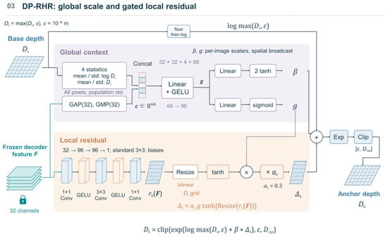
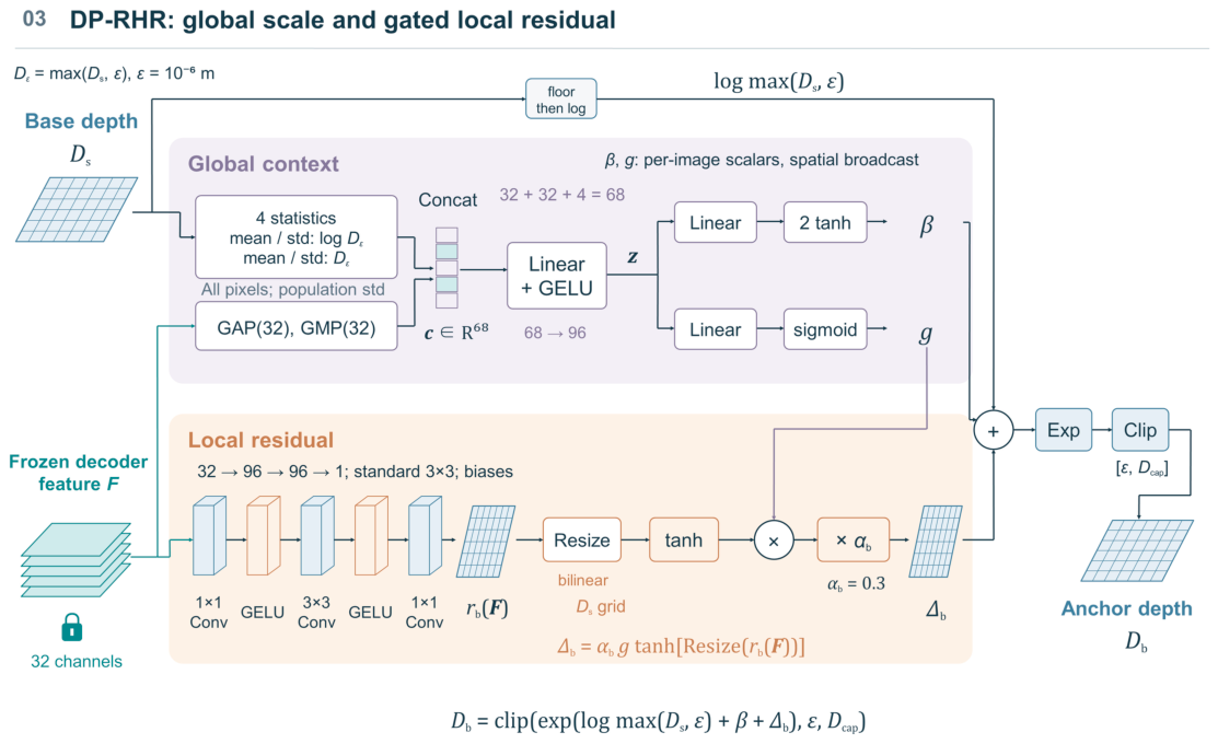
DP-RHR receives D_s and F and produces the target-domain anchor D_b. Figure 3 separates its global context branch, local residual branch and log-depth bypass. After selection, DP-RHR is frozen for RE training.

Figure 3. DP-RHR architecture.

As shown in Figure 3, the global branch of DP-RHR forms a context vector c by concatenating global average and maximum pooled values from the 32 channels of F with four statistics computed from the frozen depth prediction: the mean and population standard deviation (SD) of log D_s, and the mean and population standard deviation of D_s. Before logarithms and statistics are computed, D_s is floored at 10⁻⁶ m. These statistics are calculated over all predicted pixels rather than the reference-depth validity mask. A linear projection followed by a Gaussian error linear unit (GELU) produces the latent context representation z:

$$\begin{array}{c}\mathit{c}=\mathrm{concat}\left[\mathrm{GAP}\left(\mathit{F}\right),\mathrm{GMP}\left(\mathit{F}\right),s\left(\log D_{\mathrm{s}}\right),s\left(D_{\mathrm{s}}\right)\right]\in {\mathbb{R}}^{68}\\ \mathit{z}=\mathit{GELU}\left({\mathit{W}}_{\mathrm{c}}\mathit{c}+{\mathit{b}}_{\mathrm{c}}\right)\in {\mathbb{R}}^{96}.\end{array}$$

(5)

Here, s(·) collects the mean and population standard deviation. The projection parameters satisfy W_c ∈ ℝ^96×68 and b_c ∈ ℝ⁹⁶. Two separate linear projections of z ∈ ℝ⁹⁶, followed by bounded activations, produce the global log-scale correction β and the local-residual gate g, respectively. Both are scalars for each image and are broadcast over the spatial dimensions when combined with the local residual and depth prediction. They are computed as follows:

$$\begin{gathered} \beta ={\beta }_{\max }\tanh \left({{\mathit{w}}_{\mathsf{\beta }}}^{\mathrm{T}}\mathit{z}+b_{\mathsf{\beta }}\right),{\beta }_{\max }=2.0 \\ g=\mathrm{sigmoid}\left({{\mathit{w}}_{\mathrm{g}}}^{\mathrm{T}}\mathit{z}+b_{\mathrm{g}}\right). \end{gathered}$$

(6)

Here, w_β and w_g are the projection weights, and b_β and b_g are their scalar biases.

The local branch maps the frozen 32-channel feature F to 96 channels using a 1 × 1 convolution followed by GELU, applies a standard 3 × 3 convolution from 96 to 96 channels with GELU, and ends with a 1 × 1 convolution from 96 channels to one. All convolutions include biases. Let r_b(F) denote the resulting raw local residual field. If required, it is resized bilinearly to the D_s grid before bounding.

The local log-depth correction is calculated as follows:

Δ_b(x) = α_bg tanh[Resize(r_b(F))(x)],

(7)

where α_b = 0.3 bounds the local correction before combination with the global term. The local branch predicts an additive log-depth correction.

The image-level log-scale correction and gated local residual are combined with the base prediction to form the target-domain anchor:

D_b(x) = clip(exp[logmax(D_s(x), ε) + β + Δ_b(x)], ε, D_cap).

(8)

Here, clip(u, a, b) = min(max(u, a), b) is applied elementwise. The lower bound ε = 10⁻⁶ m is also used to floor D_s before taking the logarithm. For the selected DP-RHR anchors in the main domain-specific comparisons, the upper output bound is D_cap = 80 m; the separately trained CitrusFarm source-bag-disjoint anchors use D_cap = 30 m. These bounds define the valid output depth interval of the adapted anchor.

The final local convolution and β projection are initialized to zero. The gate projection has zero weights and bias −2, giving β = 0 and Δ_b = 0 initially. DP-RHR therefore begins with the base prediction subject to its numerical floor and output cap. It updates 93,123 parameters while the base remains frozen.

Training compares D_b with D^* on finite valid pixels in the target-domain interval. Let L_log be the mean absolute difference of natural-log depths and L_MAE the mean absolute metric-depth error. The regularizers are

L_β = mean|β|, L_res,b = mean|Δ_b|, L_gate,b = mean g.

(9)

The first and third terms average the image-level scalar values over the minibatch, whereas L_res,b averages the bounded local correction over all images and spatial positions. The residual regularizer directly penalizes the gated and bounded local correction Δ_b. The total loss is

L_DP−RHR = L_log + 0.1L_MAE + 0.001L_β + 0.01L_res,b + 0.001L_gate,b.

(10)

KITTI and NYUv2 share a DP-RHR anchor trained jointly on their training data; CitrusFarm uses a separate agricultural anchor. Each selected anchor remains fixed throughout RE training. Section 2.8 specifies optimization and checkpoint selection.

2.5. Soft Range-Expert Residual Refinement

RE models distance-dependent residual corrections to the frozen anchor. Its shared feature trunk predicts four candidate residual fields, and deterministic depth-conditioned weights combine them. The complete refined prediction is D_final.

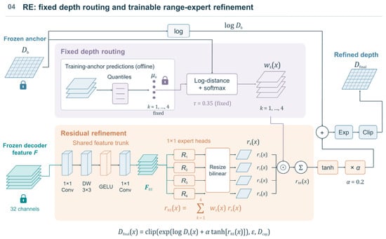
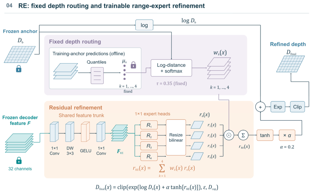
The base and DP-RHR remain frozen. Figure 4 separates routing, computed from D_b and training-derived centres, from the trainable shared trunk and expert heads. Reference depth is used for supervision, while inference-time routing uses only anchor depth.

Figure 4. Depth-conditioned range-expert refinement.

For each domain, we estimate fixed routing centres from its selected DP-RHR training-image predictions sampled on a grid with 32-pixel spacing in both spatial dimensions. We retain finite positive predicted depths no greater than the corresponding domain cap, without applying the reference-depth validity mask. Let S_train denote the pooled sample of these predicted depths, and let Quantile_q(S_train) denote its q-quantile in metres. The four centres are defined by

$$\begin{array}{c}{\mu }_k={\mathrm{Quantile}}_{q_k}\left(S_{\mathrm{train}}\right),\mathit{k}=1,2,3,4\\ \left(q_1,q_2,q_3,q_4\right)=\left(0.20,0.45,0.70,0.90\right).\end{array}$$

(11)

The four quantile levels are shared across domains, placing centres according to the training-anchor depth distribution. Soft weights depend on log-depth distance from these centres. The comparison evaluates this routing configuration as part of the complete RE module.

The resulting centres are (6.764,11.131,20.679,58.218) m for KITTI, (1.716,2.329,3.067,4.156) m for NYUv2, and (0.656,2.123,7.591,10.493) m for CitrusFarm. These values summarize the corresponding training-anchor depth distributions and remain fixed throughout RE optimization. At pixel x, w_k(x) denotes the routing weight assigned to expert k. The weights are determined by the squared distance between the frozen anchor depth D_b(x) and centre μ_k in log-depth space:

$$w_k\left(x\right)={\displaystyle \frac{\exp \left(-\frac{{\left[\log \max \left(D_{\mathrm{b}}\left(x\right),\epsilon \right) - \log {\mu }_k\right]}^2}{\tau }\right)}{{\displaystyle {\sum }_{j=1}^4}\exp \left(-\frac{{\left[\log \max \left(D_{\mathrm{b}}\left(x\right),\epsilon \right) - \log {\mu }_j\right]}^2}{\tau }\right)}},\tau =0.35,$$

(12)

where the fixed temperature τ = 0.35 controls the concentration of the soft routing distribution around nearby log-depth centres. Thus, ${\sum }_{k=1}^4{w}_k=1$ and neighbouring experts can contribute continuously without hard range boundaries. The routing weights are therefore deterministic functions of the frozen anchor depth.

As shown in Figure 4, the shared RE trunk processes F with a 32-to-32 pointwise convolution, a 32-channel depthwise 3 × 3 convolution, GELU, and a second 32-to-32 pointwise convolution to produce F_RE. All three convolutions include bias terms.

Each expert head R_k is a 1 × 1 convolution with a bias term that maps 32 channels to one. Its output is bilinearly resized to the D_b grid with aligned corners, producing the raw expert residual r_k(x). Each resized residual r_k(x) is multiplied by its corresponding routing weight, and the weighted residuals are summed across experts. In Figure 4, ⊙ denotes elementwise multiplication and Σ_k sums over the four experts. The routing-weighted residual mixture r_RE is:

$$r_{\mathrm{RE}}\left(x\right)={\displaystyle \sum _{k=1}^4}{w}_k\left(x\right)r_k\left(x\right),r_k(x)=\mathrm{Resize}[R_k({\mathit{F}}_{\mathrm{RE}})](x).$$

(13)

The mixture is bounded by α tanh(·), added to the log-anchor, exponentiated, and clipped to the domain output interval. The output of RE is refined depth D_final(x):

D_final(x) = clip(exp[logmax(D_b(x), ε) + α tanh(r_RE(x))], ε, D_cap),

(14)

where α = 0.2 bounds the additive log-depth residual, and D_cap denotes the model-side upper output cap. The RE output caps are 80 m for KITTI, 10 m for NYUv2, and 30 m for CitrusFarm. The log-depth residual is therefore bounded via α tanh(·) prior to final domain-interval clipping.

Zero initialization of the four expert heads gives r_RE = 0. The initial prediction therefore equals the floored anchor subject to the RE output cap. Section 2.6.3 evaluates this cap effect separately from learned refinement. The shared trunk and four heads contain 2564 trainable parameters; centres and temperature remain fixed.

RE uses the same valid-pixel log and metric errors as DP-RHR, with D_final as the prediction. For each minibatch, let e_b = |log D_b − log D^*| on valid pixels and t = max(Quantile_0.90(e_b), 10⁻⁶). A soft preservation weight $p=1-\min \left({\displaystyle \frac{e_{\mathrm{b}}}{t}},1\right)$ emphasizes lower-error anchor pixels. L_preserve is the valid-pixel mean of p|log D_final − log D_b|. L_gradient averages the absolute horizontal and vertical log-depth gradient discrepancies, using adjacent pairs with two valid reference pixels and averaging the available directions. The RE residual regularizer L_res,RE is the full-tensor mean of |α tanh(r_RE)|, distinct from the DP-RHR residual regularizer L_res,b. The effective objective for the trainable RE parameters is

L_RE = L_log + 0.1L_MAE + 0.1L_preserve + 0.05L_gradient + 0.01L_res,RE.

(15)

Equation (15) gives the objective acting on trainable RE parameters; Section S7 records the fixed routing diagnostic included in the scalar loss. All runs complete their fixed epoch budgets without a learning-rate scheduler. Validation AbsRel selects the checkpoint, with MAE and then higher δ₁ as tie-breakers.

2.6. Comparative Experimental Design

The comparisons address three levels of change: input preprocessing with fixed weights, the scope of target-domain adaptation, and residual refinement after freezing the anchor. Each uses a stated reference precision, support and output cap.

2.6.1. Fixed-Checkpoint Input Preprocessing

The public DAV2-S metric VKITTI checkpoint and the Stage-I base are evaluated with square and aspect-preserving inputs on the same 750 CitrusFarm test images. Both retain their 80 m model output scale. The square pipeline follows each model’s original preprocessing: OpenCV 4.10.0 area interpolation for the public checkpoint and Pillow 10.4.0 bilinear interpolation for the base. The aspect-preserving path begins with the original 1280 × 720 RGB image and uses DAV2’s cubic lower-bound resize to produce a 518 × 924 tensor. Predictions are bilinearly restored to the 518 × 518 evaluation grid with aligned corners; original FP32 reference maps are nearest-neighbour resampled. Section S10 records the additional square-interpolation check and reference-precision comparison.

Native FP32 inference is performed in PyTorch 2.5.1 with TF32 disabled. Evaluation uses a fixed support of 89,648,722 pixels with finite reference depths in [0.3, 30] m and a common 30 m output cap. Section S10 specifies the prediction-validity checks. Uncapped metrics, cap-hit fractions and mean per-image median raw prediction/reference ratios characterize the scale offset separately. The input pipelines change interpolation and pixel count as well as aspect handling.

2.6.2. Scalar Calibration and Complete Metric-Head Adaptation

Two scalar controls isolate image-independent scale calibration. LogLS minimizes squared log-depth discrepancy, and MetricLS fits a no-intercept metric-depth coefficient. Both use all 3500 training images and unclipped base predictions; the fitted coefficients are fixed for validation and test. Their objectives and coefficients are given in Section S6. Results in Section 3.2 compare those coefficients alongside the frozen base, DP-RHR and complete DPTHead using the original-FP32-reference protocol in Section 2.6.1.

The head-only control starts from the same Stage-I checkpoint and optimizes the complete original DPTHead, including multiscale projections, feature fusion and metric output layers. The encoder and auxiliary focal branch remain frozen in evaluation mode. The head updates 2,728,513 parameters within a 24,785,089-parameter depth path and retains the 80 m model output scale. It uses the same 3500 training and 750 validation images, 518 × 518 RGB preprocessing and reference support as agricultural DP-RHR adaptation. Its objective combines absolute log-depth error with 0.1 times metric MAE. This baseline directly adapts the original multiscale decoder and metric output head.

Complete-head fine-tuning uses FP32. Three runs each complete 30 epochs, batch size four and 26,250 optimizer updates, matching DP-RHR’s data and update budget. AdamW uses a validation-selected learning rate of 1 × 10⁻⁴ and weight decay of 1 × 10⁻⁴, without scheduling or augmentation. Each run starts from the same checkpoint, and minimum uncapped validation AbsRel selects the final weights. Evaluation follows the FP32-reference protocol in Section 2.6.1. Section S11 gives validation screening, per-run results and measured training time.

2.6.3. Output-Cap and Single-Head Residual Controls

To quantify the output-cap effect, we compared the original saved anchor prediction A with B(x) = clip(A(x),10⁻⁶,D_cap), with target caps of 30 m for CitrusFarm and 10 m for NYUv2. The original and capped predictions share the original finite-positive support. Clipping changes neither the predictions supplied to RE nor its routing weights. Table S1 reports both readouts across the four evaluation partitions.

For CitrusFarm, three RE runs share one selected agricultural anchor and one data split. Only the shared trunk and expert heads are optimized. Their separately selected checkpoints quantify final-stage RE optimization variability on a shared frozen anchor.

The internal-test comparison is reported in Section 3.3; Table S1 gives all four cap-control partitions and CitrusFarm validation results. Anchor rows are deterministic, and RE rows report mean ± population SD across runs. Metrics use the saved-reference protocol defined below.

The single-head comparison holds the anchor and shared feature-trunk design fixed across three methods. P2-A uses a linear 1 × 1 output head and has 2465 trainable parameters. P2-B concatenates upsampled 32-channel features with log-anchor depth, then applies a 33-to-4 projection, GELU and a 4-to-1 output head, totaling 2573 parameters. RE uses four linear heads and fixed depth routing, with 2564 parameters. Each applies the same α = 0.2 residual bound, anchor fusion and 30 m cap. P2-B’s prediction-grid nonlinear head makes this a near-parameter-matched, rather than FLOP-matched, comparison.

Cached controls store features, anchor predictions and references in FP16, promote them to FP32 for calculation, and use FP64 reductions. RE outputs are evaluated in FP32 against those references. Section S6 reports scalar controls and a separate re-evaluation of the original RE checkpoints; Section S7 reports the independently trained residual controls. These cached-input control cohorts follow the saved-reference protocol to provide a matched internal comparison.

2.7. Evaluation Metrics

Let $\widehat{D}$ be any model’s predicted metric depth, D^* the dataset-provided reference, and V the valid-pixel set specified by the relevant evaluation protocol: Section 2.2 for domain and contextual evaluations, Section 2.6.3 for cached controls, and Section 2.6.1 for FP32 full-forward comparisons. Lower values indicate better performance for absolute relative error (AbsRel), root mean squared error (RMSE), mean absolute error (MAE), and mean absolute base-10 log error E_log10; RMSE and MAE are reported in metres, whereas AbsRel and E_log10 are dimensionless. Threshold accuracy δ_k is the fraction of valid pixels whose depth ratio is below 1.25^k, for k = 1, 2, 3; higher values indicate better performance. The following dense metrics pool all valid pixels within a split:

$$\mathrm{AbsRel}={\displaystyle \frac{1}{\left|V\right|}}\sum _{x\in V}{\displaystyle \frac{\left|\widehat{D}\left(x\right)-D^{*}\left(x\right)\right|}{D^{*}\left(x\right)}},$$

(16)

$$\mathrm{RMSE}=\sqrt{{\displaystyle \frac{1}{\left|V\right|}}\sum _{x\in V}{\left(\widehat{D}\left(x\right)-D^{*}\left(x\right)\right)}^2},\mathrm{MAE}={\displaystyle \frac{1}{\left|V\right|}}\sum _{x\in V}\left|\widehat{D}\left(x\right)-D^{*}\left(x\right)\right|,$$

(17)

$$E_{\log 10}={\displaystyle \frac{1}{\left|V\right|}}\sum _{x\in V}\left|{\log }_{10}\widehat{D}\left(x\right)-{\log }_{10}{D}^{*}\left(x\right)\right|,$$

(18)

$${\delta }_k={\displaystyle \frac{1}{\left|V\right|}}\sum _{x\in V}1\left[\max \left({\displaystyle \frac{\widehat{D}\left(x\right)}{D^{*}\left(x\right)}},{\displaystyle \frac{D^{*}\left(x\right)}{\widehat{D}\left(x\right)}}\right)<{1.25}^k\right],k=1,2,3.$$

(19)

Repeated-run summaries are arithmetic mean ± population SD of separately evaluated metrics. Deterministic anchor and scalar readouts have no run SD. For the paired RE-minus-anchor analysis, each run uses 10,000 matched-image bootstrap resamples of 750 images. These intervals describe mean per-image metric differences; the primary tables instead pool valid pixels. Negative error differences favour RE. Three-fold summaries describe recording-group partitions and separately trained adapters, rather than optimizer repeats on one split.

2.8. Training and Deployment Settings

Base screening used 2100 training images (1000 Virtual KITTI 2, 1000 KITTI and 100 NYUv2) and 300 validation images (100 per source). Each configuration was trained once for 30 epochs with 518 × 518 input, a 0.001–80 m interval and AdamW at learning rate 5 × 10⁻⁶ and weight decay 0.01. Batch sizes were two, three and four for DAV2-L, DAV2-B and DAV2-S. Table S15 reports the screening results. The selected DAV2-S then received 5000 continuation updates on 44,261 images: 22,901 KITTI, 21,260 Virtual KITTI 2 and 100 NYUv2. Continuation used batch four, the same optimizer and losses, shuffled sampling and no scheduler, covering less than one pass through the list before freezing the depth path.

The shared public DP-RHR anchor used 30 epochs, AdamW at 5 × 10⁻⁵, weight decay 10⁻⁴ and batch four. Each epoch sampled 1014 training images per domain without replacement. Mean validation AbsRel over 217 images per domain selected epoch 29; results for the full 3111-image KITTI validation partition are reported in Section 3.4. CitrusFarm DP-RHR used 30 epochs, learning rate 10⁻⁴, weight decay 10⁻⁴ and batch four, with epoch 29 selected by validation AbsRel. Domain-specific RE used AdamW at 5 × 10⁻⁵, weight decay 10⁻⁴, batch eight and 20 epochs. Three runs shared each domain’s split and anchor. All runs completed their fixed training schedules, and validation performance selected the final checkpoint. The recording-group experiment retrained both correction stages for 20 epochs per fold.

For the single-head comparison, P2-A, P2-B and RE each used three FP32 training runs, 20 epochs, batch eight, AdamW at 5 × 10⁻⁵, weight decay 10⁻⁴ and no scheduler. The nine runs shared the anchor, cached data, corresponding random-seed sample orders, effective loss in Equation (15), residual bound and output cap. Checkpoint selection minimized validation AbsRel, then MAE and then maximized δ₁, retaining the earliest exact tie. Section S7 reports each selected run and all seven metrics.

Deployment accuracy uses one RE snapshot selected at epoch 15. Native PyTorch 2.5.0a0+872d972e41.nv24.08 FP32 with TF32 and autocast disabled and the TensorRT 10.7.0 FP16-enabled engine process the same 750 internal-test images with original FP32 inputs and references. Metrics pool the common finite-positive reference support in [0.3, 30] m. Section S8 identifies this snapshot and accuracy engine; Section S9 separately identifies the timing engines.

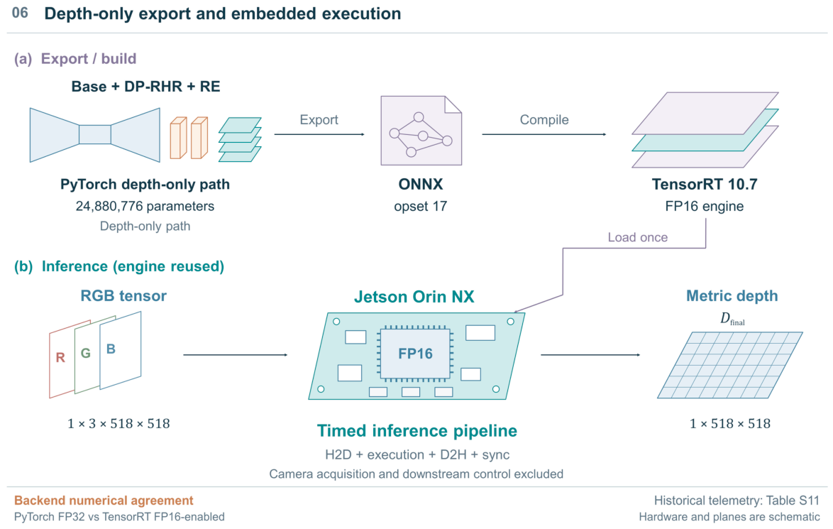
The accuracy and timing graphs were exported using ONNX 1.22.0 and 1.17.0, respectively, both with opset 17 [47]. The engines were built with TensorRT 10.7.0 [48] on the Jetson Orin NX (NVIDIA Corporation, Santa Clara, CA, USA); the runtime query reported MAXN-SUPER (mode 0) [49]. Input and output shapes were fixed to 1 × 3 × 518 × 518 and 1 × 518 × 518. The FP16 engine used batch size 1 and a 2048 MiB build-memory allocation. For the cumulative timing comparison, each configuration uses 100 warmups and three 500-iteration measurement blocks cycling eight predetermined validation inputs. Native FP32 component timing separately marks the base, DP-RHR and RE boundaries with CUDA events during the same forward pass; its intermediate tensors stay on-device and transfers are excluded. Operating conditions and engine identities are detailed in Supplementary Section S9. Explicit synchronization is used for both timing paths. Throughput in frames per second (FPS) is related to mean latency in milliseconds by:

$$\mathrm{FPS}={\displaystyle \frac{1000}{{\mathrm{latency}}_{\mathrm{ms}}}}.$$

(20)

The timed interval included host-to-device (H2D) transfer, TensorRT execution, device-to-host (D2H) transfer, and stream synchronization. Camera acquisition and camera transport, image decoding, host-side preprocessing, and downstream planning, control, and actuation were excluded.

3. Results

3.1. Scale Bias and Input Preprocessing

Aspect-preserving input left substantial overestimation in both fixed checkpoints (Table S13). Capped AbsRel changed from 7.795 to 7.974 for the public VKITTI model and from 4.782 to 4.657 for the Stage-I base. Mean image-median raw prediction/reference ratios changed from 8.08 to 8.49 and from 5.25 to 5.07, respectively. Thus the alternative pipeline modestly reduced the base’s error but did not remove its scale offset. Table S13 also gives uncapped metrics, cap-hit fractions and the square-interpolation check.

The frozen base showed a large multiplicative offset on CitrusFarm. In the original validation evaluation, its median pooled prediction/reference ratio was 5.346, with AbsRel 5.941. DP-RHR reduced the ratio to 0.965 and AbsRel to 0.317. Image-averaged absolute median log-bias fell from 1.673 to 0.101, and centred local log-residual MAE from 0.332 to 0.206. The diagnostic therefore identifies a dominant scale shift alongside spatial residual error; Section S12 retains the aggregation definitions and depth-interval results.

3.2. Scalar, Output-Side and Complete-Head Adaptation

Table 3 separates the frozen base from the correction modules. DP-RHR updates 93,123 parameters and RE updates a further 2564, totaling 95,687 added parameters. The complete depth path contains 24,880,776 parameters. The compact-base screening and auxiliary-model inventory are reported in Tables S4 and S15, respectively.

Table 3. Parameter accounting for the depth-inference path.

Depth Assembly	Added Parameters	Cumulative Depth Path	Updated in Stage
Metric-depth base (DAV2-S)	24,785,089	24,785,089	I
Base + DP-RHR	93,123	24,878,212	II
SARE-Depth (Base + DP-RHR + RE)	2564	24,880,776	III

Note: Depth Pro is an offline teacher. The auxiliary focal branch is excluded from the depth path and included separately in Table S4. Updated parameters and cumulative model size are distinct quantities.

Under common FP32-reference evaluation, a single training-fitted coefficient removed about 90% of the base AbsRel (Table 4). LogLS and MetricLS reached 0.487 and 0.476, respectively, from 4.782 for the frozen base. DP-RHR reduced AbsRel further to 0.325, 31.65% below MetricLS, while improving RMSE and δ₁. Joint image-dependent scaling and local-residual correction thus improved on image-independent scalar calibration.

Table 4. Adaptation on the CitrusFarm internal test with common FP32 references and a 30 m output cap.

Adaptation	Updated Parameters/Fitted Scalars	Depth-Path Parameters	AbsRel	RMSE (m)	δ1
Frozen base	0	24,785,089	4.782	11.194	0.016
LogLS	1 scalar	24,785,089	0.487	3.524	0.310
MetricLS	1 scalar	24,785,089	0.476	3.543	0.312
DP-RHR	93,123	24,878,212	0.325	3.138	0.673
Complete DPTHead	2,728,513	24,785,089	0.220 ± 0.006	3.036 ± 0.020	0.678 ± 0.029

Note: All rows use 750 images and 89,648,722 fixed reference pixels. The first four rows are deterministic evaluations of fixed models or training-fitted coefficients. Complete DPTHead reports mean ± population SD across three optimization runs. DP-RHR and head adaptation share the training/validation split, 30 epochs, batch four and 26,250 updates; training precision and module-specific regularization differ as specified in Section 2.6.2 and Section S11. Cached scalar readouts remain in Table S7, and individual head results in Table S14.

Complete DPTHead fine-tuning achieved the lowest AbsRel in this adaptation comparison: 0.220 ± 0.006 across three runs, with RMSE 3.036 ± 0.020 m and δ₁ 0.678 ± 0.029 (Table 4). It updated 2,728,513 parameters, 29.3 times DP-RHR’s count. The accuracy gain accompanies a larger adaptation scope. Table S14 gives the individual runs; Section 3.6 reports execution measurements for the base and correction modules.

3.3. Incremental Refinement and Residual Controls

RE produced a smaller improvement after anchor adaptation (Table 5). On the internal test, mean AbsRel decreased from 0.3252 to 0.3149 and RMSE from 3.138 to 3.093 m, reductions of 3.17% and 1.43%. Threshold accuracy δ₁ decreased from 0.6730 to 0.6699. The contextual zero-shot comparison is retained separately in Table S16, where external models and CitrusFarm-supervised models have different training regimes.

Table 5. RE increment and output-cap control on 750 CitrusFarm internal-test images.

Configuration	AbsRel	RMSE (m)	MAE (m)	δ1
Frozen DP-RHR anchor	0.3252	3.1382	1.3616	0.6730
Same anchor, 30 m output cap	0.3252	3.1382	1.3616	0.6730
SARE-Depth, three RE runs	0.3149 ± 0.0009	3.0932 ± 0.0007	1.3385 ± 0.0007	0.6699 ± 0.0004

Note: The anchor and cap-matched anchor are deterministic readouts of the same predictions. RE values are mean ± population SD across three runs with the anchor and split fixed. All rows pool 89,648,722 pixels using the saved-reference protocol in Section 2.6.3. Only the 2564 RE parameters vary between runs. Table S1 provides the complete four-partition cap comparison.

Output clipping did not explain this improvement. The largest evaluated anchor prediction was 21.56 m, below the RE cap, so the original and cap-matched anchors had identical test metrics. The learned residual stage changed predictions beyond this deterministic readout control.

Paired-image bootstrap results supported the error reduction at the image level. Across three runs, mean RE-minus-anchor AbsRel differences ranged from −0.0145 to −0.0113 and RMSE differences from −0.072 to −0.070 m; their 95% intervals were below zero. MAE and log-error differences had the same direction, while δ₁ intervals crossed zero. These are image-averaged differences from 10,000 paired resamples per run, distinct from pooled-pixel differences. Image pairing retains model correspondence but not within-bag temporal dependence; Section 3.4 examines recording-group variation.

RE also achieved lower mean AbsRel than both near-parameter-matched single-head controls (Table 6): 0.3149 ± 0.0009, versus 0.3183 ± 0.0011 for P2-A and 0.3187 ± 0.0014 for P2-B. The relative gains were 1.06% and 1.18%, with the same direction in each corresponding run. Six of seven mean metrics favoured RE; δ₁ was lower than both single-head controls and the anchor. This comparison concerns a separate three-run cohort on the shared cached inputs defined in Section 2.6.3.

Table 6. Near-parameter-matched residual controls on the CitrusFarm internal test.

Trainable Refinement	Trainable Parameters	AbsRel	RMSE (m)	δ1
P2-A: single linear head	2465	0.3183 ± 0.0011	3.1006 ± 0.0022	0.6701 ± 0.0007
P2-B: depth-conditioned head	2573	0.3187 ± 0.0014	3.1091 ± 0.0065	0.6700 ± 0.0002
RE: four routed heads	2564	0.3149 ± 0.0009	3.0932 ± 0.0007	0.6699 ± 0.0004

Note: Mean ± population SD over three FP32 training runs per method, sharing the anchor, cached inputs, sample orders, budget, loss and cap. Each readout pools 89,648,722 pixels over 750 images. FP16 storage of features, depth and references precedes FP32 computation. P2-B’s upsampled nonlinear head has a different computational structure. Table S9 gives per-run values and all seven metrics.

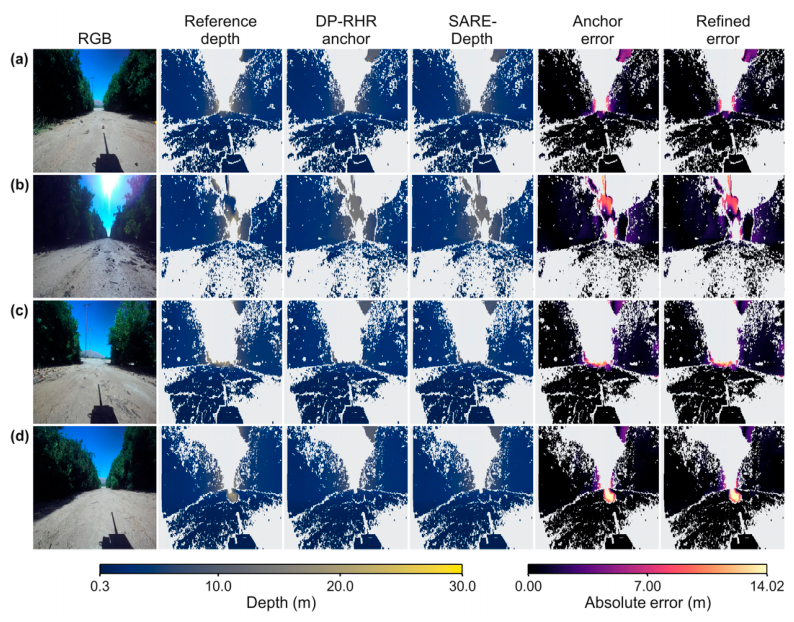
Figure 5 illustrates local depth and absolute-error differences for four internal-test images using one selected anchor and RE run.

Figure 5. CitrusFarm internal-test depth comparisons. Columns show RGB, registered reference depth, DP-RHR, SARE-Depth and the two absolute-error maps. Rows (a–d) are selected examples; grey denotes invalid reference depth. Depth panels share a 0.3–30 m scale and error panels a 0.00–14.02 m scale.

For rows (a–d), anchor/RE AbsRel values were 0.142/0.137, 0.374/0.357, 0.154/0.154 and 0.104/0.106. The examples show spatially heterogeneous changes, including a small increase in the final row.

3.4. Domain and Recording-Group Variation

Refinement gains varied across domains (Table 7). KITTI and NYUv2 shared one public-data anchor, while CitrusFarm used its agricultural anchor. On KITTI validation, RE reduced AbsRel by 8.36% and RMSE by 0.42%; the three AbsRel values spanned 0.0821–0.0823. Improved relative error and δ₁ accompanied a small decrease in δ₃.

Table 7. Domain-specific validation of DP-RHR anchors and separately trained RE modules.

Domain/Model	AbsRel	RMSE (m)	MAE (m)	Elog10	δ1	δ2	δ3
Shared public DP-RHR anchor (KITTI)	0.0897	3.6173	1.6933	0.0386	0.9303	0.9868	0.9962
KITTI SARE-Depth	0.0822 ± 0.0001	3.6020 ± 0.0024	1.6274 ± 0.0021	0.0360 ± 0.0001	0.9362 ± 0.0003	0.9868 ± 0.0001	0.9959 ± <0.0001
Shared public DP-RHR anchor (NYUv2)	0.1840	0.8273	0.5401	0.0798	0.6864	0.9328	0.9884
NYUv2 SARE-Depth	0.1840 ± <0.0001	0.8222 ± 0.0007	0.5376 ± 0.0003	0.0794 ± <0.0001	0.6897 ± 0.0003	0.9334 ± 0.0001	0.9885 ± <0.0001
CitrusFarm DP-RHR anchor	0.3174	2.1148	1.0604	0.1004	0.6375	0.8904	0.9543
CitrusFarm SARE-Depth	0.2995 ± 0.0003	2.0556 ± 0.0017	1.0355 ± 0.0007	0.0989 ± 0.0001	0.6414 ± 0.0003	0.8893 ± 0.0001	0.9552 ± 0.0001

Note: Values follow the domain-specific evaluation in Section 2.2. RE results are mean ± population SD over three training runs; anchors are deterministic. KITTI and NYUv2 evaluate the same public-data anchor under their domain protocols. CitrusFarm uses a separate agricultural anchor. Each domain has its own RE parameters and training-derived centres. Nonzero SDs below 0.0001 are shown as <0.0001. Higher-precision values are retained in the evaluation records.

On NYUv2 validation, reductions in RMSE and MAE accompanied higher threshold accuracy, but each RE run had higher AbsRel than the 10 m cap-matched anchor (Table S1). The original-anchor comparison alone therefore overstates the AbsRel benefit of refinement.

The 218-image NYUv2 held-out test showed the same metric-dependent pattern on 58,494,632 common pixels. AbsRel increased from 0.1847 to 0.1851, while RMSE decreased from 0.7727 to 0.7699 m and δ₁ increased from 0.6962 to 0.6988. The cap-matched anchor also had lower AbsRel than every RE run, and δ₃ declined after refinement. Table S1 reports all seven metrics and their run variability.

CitrusFarm validation showed a 5.64% reduction in mean AbsRel, together with improved RMSE, MAE and δ₁ (Table 7). The corresponding internal-test δ₁ decreased (Table 5), showing that the direction of threshold-accuracy change depended on the evaluation partition.

Mean routing weights were distributed across the four experts: maximum weights were 0.282, 0.280 and 0.327 for KITTI, NYUv2 and CitrusFarm, with entropies 1.382, 1.378 and 1.355 against log 4 = 1.386. The diagnostic computes entropy after spatial and batch averaging, H(mean w), rather than mean pixel entropy. Fewer than 0.13% of sampled residuals reached 95% of the allowed amplitude. These diagnostics show broadly distributed mean routing weights and infrequent near-saturation of the bounded residual correction.

Recording-group evaluation produced mixed AbsRel changes (Table 8). Across the three source-bag folds, mean AbsRel changed from 0.314 to 0.313 and RMSE from 2.260 to 2.215 m. RE improved AbsRel in fold 1 but increased it in folds 2 and 3; RMSE decreased in all folds, and δ₁ decreased in fold 2. Table S2 gives each fold’s anchor, RE and paired difference under the distinct 20-epoch, 30 m cap protocol in Section 2.2.

Table 8. Three-fold CitrusFarm source-bag-disjoint evaluation.

Model	AbsRel	RMSE (m)	MAE (m)	Elog10	δ1	δ2	δ3
DP-RHR anchor	0.314 ± 0.044	2.260 ± 0.023	1.126 ± 0.028	0.093 ± 0.005	0.708 ± 0.030	0.891 ± 0.011	0.952 ± 0.003
SARE-Depth	0.313 ± 0.047	2.215 ± 0.053	1.111 ± 0.035	0.092 ± 0.005	0.708 ± 0.028	0.894 ± 0.012	0.953 ± 0.004

Note: Arithmetic mean ± population SD across three recording-file folds, with the same displayed decimal place for each mean and its SD.

3.5. Dingxi Object-Distance Measurements

The six Dingxi examples in Figure S1 show underestimation by both frozen models. Their recorded reference distances span 1.801–8.135 m, compared with DP-RHR ROI medians of 0.712–3.004 m and RE medians of 0.696–2.958 m. RE lowers the prediction in each displayed example, increasing the magnitude of its negative signed error. Tables S5 and S6 give the record-level distances and errors; Section S5 describes measurement correspondence and model provenance.

3.6. Embedded Inference

The two deployment backends produced close numerical agreement over all 750 internal-test images (Table 9). Both had AbsRel 0.3137 at four-decimal display precision; TensorRT minus native FP32 was +1.10 × 10⁻⁵ before rounding. Slightly lower RMSE and MAE on TensorRT accompany this small combined backend-and-precision difference for one selected snapshot. Figure 6 shows the depth-only export and execution path.

Table 9. Full-internal-test accuracy of one fixed deployment snapshot.

Metric	Native FP32	TensorRT FP16-Enabled	TRT Minus Native
AbsRel	0.3137	0.3137	+1.10 × 10−5
RMSE (m)	3.0930	3.0930	−2.02 × 10−5
MAE (m)	1.3389	1.3387	−1.94 × 10−4

Note: Both backends use the same 750 images, original FP32 references and 89,648,722 valid pixels. The RE checkpoint was selected at epoch 15. Signed differences are calculated before rounding. Section S8 reports full metrics and engine identities; Section S9 describes the timing engines.

Figure 6. Depth-only export and embedded execution of SARE-Depth.

Across 89,648,722 common pixels, absolute prediction differences averaged 0.004 m, with median 0.002 m, 95th percentile 0.015 m and maximum 0.633 m. Mean relative difference was 0.164%. Section S8 provides higher-precision summaries and identifies the accuracy engine separately from the timing engines.

Adding the correction modules increased cumulative TensorRT latency (Table 10). Mean latency was 26.87 ms for the base, 31.49 ms with DP-RHR and 35.08 ms with RE. The compiled-path increments were 4.61 ms for DP-RHR and 3.59 ms for RE, or 17.2% and 11.4% relative to their respective preceding paths. The complete graph took 30.5% longer than the base under the same eight-input timing protocol.

Table 10. Cumulative TensorRT pipeline timings under recorded operating conditions.

Configuration	Mean (ms)	Median (ms)	SD (ms)	p95 (ms)	1000/Mean (s−1)
J0: base	26.87	27.08	0.72	27.92	37.2
J1: base + DP-RHR	31.49	31.48	0.19	31.88	31.8
J2: base + DP-RHR + RE	35.08	34.86	0.74	36.50	28.5

Note: Each row contains 1500 synchronized measurements after 100 warmups, under dynamic operating conditions with MAXN-SUPER mode reported by the device. Rates are inverse mean latency. Supplementary Section S9 reports both timing sessions and their telemetry.

Native PyTorch 2.5.0a0+872d972e41.nv24.08 FP32 component means were 344.21 ms for base depth and features, 48.21 ms for DP-RHR and 12.13 ms for RE; single-pass total latency was 404.54 ms. These device-only CUDA-event measurements exclude transfers, whereas the TensorRT interval includes host/device transfers and synchronization. Section S9 reports both timing sessions and their measurement boundaries.

4. Discussion

4.1. Adaptation Scope and the Source of Scale Bias

The adaptation comparison distinguishes image-independent scale calibration from joint image-dependent scaling and local residual correction. One coefficient removed about 90% of base AbsRel. DP-RHR then closed approximately 59% of the remaining AbsRel gap between MetricLS and complete-head fine-tuning, using 3.4% as many updated parameters. Complete DPTHead achieved the lowest AbsRel, whereas DP-RHR retained the base weights and learned modular output corrections. Complete DPTHead fine-tuning updates decoder-head weights in place within the 24,785,089-parameter depth path, preserving the J0 base’s inference-graph topology and tensor dimensions without additional branches. It updates 29.3 times as many parameters as DP-RHR, which adapts the frozen base through 93,123 correction parameters at a measured cumulative TensorRT latency increment of 4.61 ms (Section 3.6).

Substantial overestimation persisted with aspect-preserving input. This comparison changes interpolation and pixel count together with aspect handling, testing two input pipelines rather than one isolated factor. CitrusFarm’s Jackal/ZED platform differs from the road-vehicle viewpoints in KITTI and KITTI-derived Virtual KITTI scenes [42,44,45]. Camera height and pitch change the ground-plane distance associated with an image location; field of view and scene structure also change the available geometric cues. A camera-height prior above the actual mounting height could therefore contribute to overestimated ground distances. The stronger overestimation of the unmodified public VKITTI checkpoint under both input pipelines shows that the scale offset predates Stage-I continuation. This pattern is consistent with differences in camera geometry and scene structure between road-vehicle pretraining and orchard imagery.

4.2. The Incremental Role of Range Experts

RE addresses the residual error after anchor formation. Its advantage over the cap-matched anchor and the two single-head alternatives is smaller than the initial adaptation gain and depends on the metric. The four linear heads constitute an anchor-depth-dependent linear readout of shared features. The controls support the value of that complete routed readout over the specified alternatives, while centre placement, soft routing and residual preservation remain coupled design choices.

This final refinement is optional in deployment. On the CitrusFarm internal test, RE improves relative error but reduces δ₁. It adds 3.59 ms to the cumulative TensorRT path. NYUv2 shows no AbsRel advantage over the cap-matched anchor, while recording-group folds show mixed AbsRel changes. Together, these results make refinement selection a domain- and metric-dependent decision rather than an automatic consequence of its small parameter count.

4.3. Agricultural Evidence and Measurement Correspondence

The data-quantity experiments compare sequential adaptation with refinement over a full-data anchor (Section S3). Their non-monotonic fixed-anchor trend occurs alongside changing source-bag composition. Recording-group folds expose that variation directly by retraining both adapters within file-group partitions, whereas repeated RE runs measure optimization variability with one fixed anchor and split.

Agricultural evidence combines dense CitrusFarm evaluation with separate-location Dingxi object-distance examples. The CitrusFarm internal test shares recording-file provenance with validation, while its group folds partition files within the same collection. The Dingxi collection comprises 495 field images: 220 calibration-board and 275 blue-box images. Its six illustrated targets provide external object-distance spot checks using the selected, frozen CitrusFarm models (Section S5).

The field records provide laser-derived object-distance references, whereas the ROI median summarizes the predicted target region. The six examples show underestimation relative to those references. These target-specific comparisons complement the dense orchard evaluation through external object-distance sampling, whereas full-image dense validation across multiple independent farms and acquisition sessions remains an important direction for future work.

4.4. Embedded Execution and Agricultural Use

The backend comparison shows close average numerical agreement for one fixed deployment snapshot. Cumulative TensorRT timing includes transfers and inference, while native component measurements isolate device execution. Headland use depends on boundary-distance tolerance, approach speed and stopping distance. At a true distance of 10 m, the δ₁ criterion accepts predictions strictly between 8 and 12.5 m. Pooled δ₁ of approximately 0.67 therefore describes pixel-depth agreement over a broad distance interval, not the accuracy of a row-end decision. Relating depth to a turning or deceleration threshold requires measured boundary and decision errors at the intended operating speed.

5. Conclusions

SARE-Depth adapts a frozen metric-depth predictor through joint global-scale and local-residual correction, followed by optional depth-conditioned refinement. On CitrusFarm, scalar calibration explains much of the base error; DP-RHR provides further correction with 93,123 updated parameters, while complete DPTHead fine-tuning reaches lower AbsRel by updating 2,728,513 parameters.

RE provides a smaller increment over the anchor and single-head residual controls, with lower threshold accuracy and additional execution time. The benefit of refinement varies across the evaluated domains and recording groups. Dingxi examples show object-distance underestimation at a separate location, and the Jetson measurements quantify the cost of the complete depth path. These results support choosing adaptation scope jointly from measured accuracy, update count and application-specific timing needs.

References

- Bechar, A.; Vigneault, C. Agricultural robots for field operations: Concepts and components. Biosyst. Eng. 2016, 149, 94–111. [Google Scholar] [CrossRef] [Scilit]
- Shamshiri, R.R.; Weltzien, C.; Hameed, I.A.; Yule, I.J.; Grift, T.E.; Balasundram, S.K.; Pitonakova, L.; Ahmad, D.; Chowdhary, G. Research and development in agricultural robotics: A perspective of digital farming. Int. J. Agric. Biol. Eng. 2018, 11, 1–14. [Google Scholar] [CrossRef]
- Bai, Y.; Zhang, B.; Xu, N.; Zhou, J.; Shi, J.; Diao, Z. Vision-based navigation and guidance for agricultural autonomous vehicles and robots: A review. Comput. Electron. Agric. 2023, 205, 107584. [Google Scholar] [CrossRef] [Scilit]
- Bac, C.W.; van Henten, E.J.; Hemming, J.; Edan, Y. Harvesting Robots for High-value Crops: State-of-the-art Review and Challenges Ahead. J. Field Robot. 2014, 31, 888–911. [Google Scholar] [CrossRef] [Scilit]
- Botta, A.; Cavallone, P.; Baglieri, L.; Colucci, G.; Tagliavini, L.; Quaglia, G. A Review of Robots, Perception, and Tasks in Precision Agriculture. Appl. Mech. 2022, 3, 830–854. [Google Scholar] [CrossRef] [Scilit]
- Sa, I.; Ge, Z.; Dayoub, F.; Upcroft, B.; Perez, T.; McCool, C. DeepFruits: A Fruit Detection System Using Deep Neural Networks. Sensors 2016, 16, 1222. [Google Scholar] [CrossRef] [Scilit] [PubMed]
- Milioto, A.; Lottes, P.; Stachniss, C. Real-Time Semantic Segmentation of Crop and Weed for Precision Agriculture Robots Leveraging Background Knowledge in CNNs. In Proceedings of the 2018 IEEE International Conference on Robotics and Automation (ICRA), Brisbane, Australia, 21–25 May 2018; pp. 2229–2235. [Google Scholar] [CrossRef] [Scilit]
- Gai, J.; Xiang, L.; Tang, L. Using a depth camera for crop row detection and mapping for under-canopy navigation of agricultural robotic vehicle. Comput. Electron. Agric. 2021, 188, 106301. [Google Scholar] [CrossRef] [Scilit]
- Kitzler, F.; Barta, N.; Neugschwandtner, R.W.; Gronauer, A.; Motsch, V. WE3DS: An RGB-D Image Dataset for Semantic Segmentation in Agriculture. Sensors 2023, 23, 2713. [Google Scholar] [CrossRef] [Scilit] [PubMed]
- Cui, X.-Z.; Feng, Q.; Wang, S.-Z.; Zhang, J.-H. Monocular Depth Estimation with Self-Supervised Learning for Vineyard Unmanned Agricultural Vehicle. Sensors 2022, 22, 721. [Google Scholar] [CrossRef] [Scilit] [PubMed]
- Divyanth, L.G.; Rathore, D.; Senthilkumar, P.; Patidar, P.; Zhang, X.; Karkee, M.; Machavaram, R.; Soni, P. Estimating depth from RGB images using deep-learning for robotic applications in apple orchards. Smart Agric. Technol. 2023, 6, 100345. [Google Scholar] [CrossRef] [Scilit]
- Mao, Y.; Zhao, W.; Chen, L. Parameter-Efficient Domain Adaptation and Lightweight Decoding for Agricultural Monocular Depth Estimation. Agronomy 2026, 16, 972. [Google Scholar] [CrossRef] [Scilit]
- Eigen, D.; Puhrsch, C.; Fergus, R. Depth Map Prediction from a Single Image using a Multi-Scale Deep Network. Adv. Neural Inf. Process. Syst. 2014, 27, 2366–2374. [Google Scholar] [CrossRef] [Scilit]
- Laina, I.; Rupprecht, C.; Belagiannis, V.; Tombari, F.; Navab, N. Deeper Depth Prediction with Fully Convolutional Residual Networks. In Proceedings of the 2016 Fourth International Conference on 3D Vision (3DV), Stanford, CA, USA, 25–28 October 2016; pp. 239–248. [Google Scholar] [CrossRef] [Scilit]
- Fu, H.; Gong, M.; Wang, C.; Batmanghelich, K.; Tao, D. Deep Ordinal Regression Network for Monocular Depth Estimation. In Proceedings of the 2018 IEEE/CVF Conference on Computer Vision and Pattern Recognition, Salt Lake City, UT, USA, 18–22 June 2018; pp. 2002–2011. [Google Scholar] [CrossRef] [Scilit] [PubMed]
- Godard, C.; Mac Aodha, O.; Brostow, G.J. Unsupervised Monocular Depth Estimation with Left-Right Consistency. In Proceedings of the 2017 IEEE Conference on Computer Vision and Pattern Recognition (CVPR), Honolulu, HI, USA, 21–26 July 2017; pp. 6602–6611. [Google Scholar] [CrossRef] [Scilit]
- Godard, C.; Mac Aodha, O.; Firman, M.; Brostow, G.J. Digging Into Self-Supervised Monocular Depth Estimation. In Proceedings of the 2019 IEEE/CVF International Conference on Computer Vision (ICCV), Seoul, Republic of Korea, 27 October–2 November 2019; pp. 3827–3837. [Google Scholar] [CrossRef] [Scilit]
- Ranftl, R.; Lasinger, K.; Hafner, D.; Schindler, K.; Koltun, V. Towards Robust Monocular Depth Estimation: Mixing Datasets for Zero-Shot Cross-Dataset Transfer. IEEE Trans. Pattern Anal. Mach. Intell. 2022, 44, 1623–1637. [Google Scholar] [CrossRef] [Scilit] [PubMed]
- Ranftl, R.; Bochkovskiy, A.; Koltun, V. Vision Transformers for Dense Prediction. In Proceedings of the 2021 IEEE/CVF International Conference on Computer Vision (ICCV), Virtual, 11–17 October 2021; pp. 12159–12168. [Google Scholar] [CrossRef] [Scilit]
- Yang, L.; Kang, B.; Huang, Z.; Xu, X.; Feng, J.; Zhao, H. Depth Anything: Unleashing the Power of Large-Scale Unlabeled Data. In Proceedings of the 2024 IEEE/CVF Conference on Computer Vision and Pattern Recognition (CVPR), Seattle, WA, USA, 17–21 June 2024; pp. 10371–10381. [Google Scholar] [CrossRef] [Scilit]
- Yang, L.; Kang, B.; Huang, Z.; Zhao, Z.; Xu, X.; Feng, J.; Zhao, H. Depth Anything V2. Adv. Neural Inf. Process. Syst. 2024, 37, 21875–21911. [Google Scholar] [CrossRef] [Scilit]
- Bhat, S.F.; Alhashim, I.; Wonka, P. AdaBins: Depth Estimation Using Adaptive Bins. In Proceedings of the 2021 IEEE/CVF Conference on Computer Vision and Pattern Recognition (CVPR), Virtual, 19–25 June 2021; pp. 4008–4017. [Google Scholar] [CrossRef] [Scilit]
- Bhat, S.F.; Birkl, R.; Wofk, D.; Wonka, P.; Müller, M. ZoeDepth: Zero-shot Transfer by Combining Relative and Metric Depth. arXiv 2023, arXiv:2302.12288. [Google Scholar] [CrossRef] [Scilit]
- Yin, W.; Zhang, C.; Chen, H.; Cai, Z.; Yu, G.; Wang, K.; Chen, X.; Shen, C. Metric3D: Towards Zero-shot Metric 3D Prediction from A Single Image. In Proceedings of the 2023 IEEE/CVF International Conference on Computer Vision (ICCV), Paris, France, 2–6 October 2023; pp. 9009–9019. [Google Scholar] [CrossRef] [Scilit]
- Hu, M.; Yin, W.; Zhang, C.; Cai, Z.; Long, X.; Chen, H.; Wang, K.; Yu, G.; Shen, C.; Shen, S. Metric3D v2: A Versatile Monocular Geometric Foundation Model for Zero-Shot Metric Depth and Surface Normal Estimation. IEEE Trans. Pattern Anal. Mach. Intell. 2024, 46, 10579–10596. [Google Scholar] [CrossRef] [Scilit] [PubMed]
- Bochkovskii, A.; Delaunoy, A.; Germain, H.; Santos, M.; Zhou, Y.; Richter, S.R.; Koltun, V. Depth Pro: Sharp Monocular Metric Depth in Less Than a Second. In Proceedings of the International Conference on Learning Representations (ICLR), Singapore, 24–28 April 2025; Available online: https://proceedings.iclr.cc/paper_files/paper/2025/hash/bc8b2058fd96978a4146f18298cb2d39-Abstract-Conference.html (accessed on 3 October 2026).
- Guo, Y.; Garg, S.; Miangoleh, S.M.H.; Huang, X.; Ren, L. Depth Any Camera: Zero-Shot Metric Depth Estimation from Any Camera. In Proceedings of the 2025 IEEE/CVF Conference on Computer Vision and Pattern Recognition (CVPR), Nashville, TN, USA, 11–15 June 2025; pp. 26996–27006. [Google Scholar] [CrossRef] [Scilit]
- Ganesan, G.C.; Guo, Y.; Ren, L.; Liu, X. UniDAC: Universal Metric Depth Estimation for Any Camera. In Proceedings of the IEEE/CVF Conference on Computer Vision and Pattern Recognition (CVPR), Denver, CO, USA, 3–7 June 2026; pp. 26953–26963. Available online: https://openaccess.thecvf.com/content/CVPR2026/html/Ganesan_UniDAC_Universal_Metric_Depth_Estimation_for_Any_Camera_CVPR_2026_paper.html (accessed on 3 October 2026).
- Ke, B.; Obukhov, A.; Huang, S.; Metzger, N.; Daudt, R.C.; Schindler, K. Repurposing Diffusion-Based Image Generators for Monocular Depth Estimation. In Proceedings of the 2024 IEEE/CVF Conference on Computer Vision and Pattern Recognition (CVPR), Seattle, WA, USA, 17–21 June 2024; pp. 9492–9502. [Google Scholar] [CrossRef] [Scilit]
- Cui, B.; Huang, Y.; Bai, L.; Ren, H. TR2M: Transferring Monocular Relative Depth to Metric Depth with Language Descriptions and Dual-Level Scale-Oriented Contrast. In Proceedings of the IEEE/CVF Conference on Computer Vision and Pattern Recognition (CVPR), Denver, CO, USA, 3–7 June 2026; pp. 34181–34192. Available online: https://openaccess.thecvf.com/content/CVPR2026/html/Cui_TR2M_Transferring_Monocular_Relative_Depth_to_Metric_Depth_with_Language_CVPR_2026_paper.html (accessed on 3 October 2026).
- Hinton, G.; Vinyals, O.; Dean, J. Distilling the Knowledge in a Neural Network. arXiv 2015, arXiv:1503.02531. [Google Scholar] [CrossRef] [Scilit]
- Pilzer, A.; Lathuilière, S.; Sebe, N.; Ricci, E. Refine and Distill: Exploiting Cycle-Inconsistency and Knowledge Distillation for Unsupervised Monocular Depth Estimation. In Proceedings of the 2019 IEEE/CVF Conference on Computer Vision and Pattern Recognition (CVPR), Long Beach, CA, USA, 16–20 June 2019; pp. 9760–9769. [Google Scholar] [CrossRef] [Scilit]
- Romero, A.; Ballas, N.; Kahou, S.E.; Chassang, A.; Gatta, C.; Bengio, Y. FitNets: Hints for Thin Deep Nets. In Proceedings of the International Conference on Learning Representations (ICLR), San Diego, CA, USA, 7–9 May 2015; Available online: https://arxiv.org/abs/1412.6550v4 (accessed on 4 November 2026).
- Zagoruyko, S.; Komodakis, N. Paying More Attention to Attention: Improving the Performance of Convolutional Neural Networks via Attention Transfer. In Proceedings of the International Conference on Learning Representations (ICLR), Toulon, France, 24–26 April 2017; Available online: https://openreview.net/forum?id=Sks9_ajex (accessed on 4 November 2026).
- Howard, A.G.; Zhu, M.; Chen, B.; Kalenichenko, D.; Wang, W.; Weyand, T.; Andreetto, M.; Adam, H. MobileNets: Efficient Convolutional Neural Networks for Mobile Vision Applications. arXiv 2017, arXiv:1704.04861. [Google Scholar] [CrossRef] [Scilit]
- Wofk, D.; Ma, F.; Yang, T.-J.; Karaman, S.; Sze, V. FastDepth: Fast Monocular Depth Estimation on Embedded Systems. In Proceedings of the 2019 International Conference on Robotics and Automation (ICRA), Montréal, QC, Canada, 20–24 May 2019; pp. 6101–6108. [Google Scholar] [CrossRef] [Scilit]
- Rebuffi, S.-A.; Bilen, H.; Vedaldi, A. Learning multiple visual domains with residual adapters. Adv. Neural Inf. Process. Syst. 2017, 30, 506–516. [Google Scholar] [CrossRef] [Scilit]
- Hu, E.J.; Shen, Y.; Wallis, P.; Allen-Zhu, Z.; Li, Y.; Wang, S.; Wang, L.; Chen, W. LoRA: Low-Rank Adaptation of Large Language Models. In Proceedings of the International Conference on Learning Representations (ICLR), Virtual, 25–29 April 2022; Available online: https://openreview.net/forum?id=nZeVKeeFYf9 (accessed on 4 November 2026).
- Chen, S.; Ge, C.; Tong, Z.; Wang, J.; Song, Y.; Wang, J.; Luo, P. AdaptFormer: Adapting Vision Transformers for Scalable Visual Recognition. Adv. Neural Inf. Process. Syst. 2022, 35, 16664–16678. [Google Scholar] [CrossRef] [Scilit]
- Jacobs, R.A.; Jordan, M.I.; Nowlan, S.J.; Hinton, G.E. Adaptive Mixtures of Local Experts. Neural Comput. 1991, 3, 79–87. [Google Scholar] [CrossRef] [Scilit] [PubMed]
- Shazeer, N.; Mirhoseini, A.; Maziarz, K.; Davis, A.; Le, Q.; Hinton, G.; Dean, J. Outrageously Large Neural Networks: The Sparsely-Gated Mixture-of-Experts Layer. In Proceedings of the International Conference on Learning Representations (ICLR), Toulon, France, 24–26 April 2017; Available online: https://openreview.net/forum?id=B1ckMDqlg (accessed on 4 November 2026).
- Geiger, A.; Lenz, P.; Urtasun, R. Are we ready for autonomous driving? The KITTI vision benchmark suite. In Proceedings of the 2012 IEEE Conference on Computer Vision and Pattern Recognition (CVPR), Providence, RI, USA, 16–21 June 2012; pp. 3354–3361. [Google Scholar] [CrossRef] [Scilit]
- Silberman, N.; Hoiem, D.; Kohli, P.; Fergus, R. Indoor Segmentation and Support Inference from RGBD Images. In Computer Vision—ECCV 2012; Lecture Notes in Computer Science; Springer: Berlin/Heidelberg, Germany, 2012; Volume 7576, pp. 746–760. [Google Scholar] [CrossRef] [Scilit]
- Teng, H.; Wang, Y.; Song, X.; Karydis, K. Multimodal Dataset for Localization, Mapping and Crop Monitoring in Citrus Tree Farms. In Advances in Visual Computing, ISVC 2023; Lecture Notes in Computer Science; Springer: Cham, Switzerland, 2023; Volume 14361, pp. 571–582. [Google Scholar] [CrossRef] [Scilit]
- Cabon, Y.; Murray, N.; Humenberger, M. Virtual KITTI 2. arXiv 2020, arXiv:2001.10773. [Google Scholar] [CrossRef] [Scilit]
- Oquab, M.; Darcet, T.; Moutakanni, T.; Vo, H.V.; Szafraniec, M.; Khalidov, V.; Fernandez, P.; Haziza, D.; Massa, F.; El-Nouby, A.; et al. DINOv2: Learning Robust Visual Features without Supervision. Transactions on Machine Learning Research 2024. Available online: https://openreview.net/forum?id=a68SUt6zFt (accessed on 4 November 2026).
- ONNX Project. ONNX Versioning; Documentation Snapshot for Release v1.12.0. 2022. Available online: https://github.com/onnx/onnx/blob/v1.12.0/docs/Versioning.md (accessed on 3 October 2026).
- NVIDIA. TensorRT 10.7.0 Release Notes. Available online: https://docs.nvidia.com/deeplearning/tensorrt/10.x.x/getting-started/release-notes-10/10.7.0.html (accessed on 3 October 2026).
- NVIDIA. JetPack 6.2 Release Notes. 2025. Available online: https://docs.nvidia.com/jetson/jetpack/6.2/release-notes/index.html (accessed on 3 October 2026).
Disclaimer/Publisher’s Note: The statements, opinions and data contained in all publications are solely those of the individual author(s) and contributor(s) and not of MDPI and/or the editor(s). MDPI and/or the editor(s) disclaim responsibility for any injury to people or property resulting from any ideas, methods, instructions or products referred to in the content. |
© 2026 by the authors. Licensee MDPI, Basel, Switzerland. This article is an open access article distributed under the terms and conditions of the Creative Commons Attribution (CC BY) license.