


Abstract
Continuously acquired garlic images can contain temporally related observations that affect soil residue grading estimates. This study assessed data-partitioning sensitivity and within-session acquisition-stage transfer using a two-stage You Only Look Once version 26 nano (YOLO26n) detector and EfficientNet-B0 classifier. The dataset comprised 754 red–green–blue (RGB) scene images and 10,721 bulb instances collected during one controlled session in which the conveyor operated at 0.5 m/s, while active vibratory soil removal was disabled (0 Hz vibration frequency and 0° screen inclination); inter-annotator agreement was high (quadratic-weighted Cohen’s κ = 0.8750; 360 instances). For seed 42, macro-averaged F1-score (Macro-F1) was 97.49% with random image splitting, 87.43% with 2 s temporal exclusion, and 76.32% with complete stage isolation. Three additional temporal-exclusion runs yielded 85.92 ± 1.38% Macro-F1. On a fixed S07 test set (26 scenes, 405 bulbs), replacing temporally neighboring training images with more distant same-stage images, while preserving training-scene and class-specific instance counts, changed Macro-F1 from 99.76% to 74.12%. In a three-seed, four-fold leave-one-stage-out (LOSO) evaluation, stage-based group distributionally robust optimization (Stage-GroupDRO) achieved 75.57% Stage-macro Macro-F1 versus 74.11% for class-weighted empirical risk minimization (Weighted-ERM), but the paired 95% confidence interval included zero. The full pipeline achieved 72.82% pooled end-to-end Macro-F1 at 19.32 frames per second (FPS) during offline evaluation. These results demonstrate substantial sensitivity to data partitioning within one acquisition session; external generalization, quantitative soil-removal efficiency, and closed-loop control remain untested.
1. Introduction
Mechanized garlic harvesting and postharvest soil removal involve digging, conveying, soil separation, root and stem treatment, and collection. Forward speed, digging depth, conveying conditions, and separation intensity affect residual soil, product loss, and bulb damage [1,2,3,4,5]. Insufficient soil removal increases the burden on subsequent handling, whereas excessive vibration, impact, or friction can increase mechanical injury. Machine vision has been applied to garlic root-trimming assessment, autonomous grading and sorting, and adaptive root-cutting control [6,7,8]. Extending visual perception to soil residue grading could provide a useful state signal for adjusting conveying speed, vibration frequency, or screen inclination during soil removal.
Machine vision is now widely used for agricultural detection, grading, sorting, and robotic handling, with real-time applications reported for watermelon seeds, sweet potatoes, fresh tea leaves, and soybean defects [9,10,11,12]. Reviews of deep-learning and You Only Look Once (YOLO)-based agricultural vision systems further show that practical performance depends not only on model architecture, but also on dataset construction, validation design, computational cost, and deployment conditions [13,14]. Continuous-image acquisition adds another important consideration because successive observations may be strongly related rather than statistically independent.
For visible soil residue grading, the choice of vision architecture should consider both multi-object localization and the discrimination of subtle soil-coverage differences on individual garlic bulbs. A single-stage multiclass detector can jointly localize bulbs and predict residue grades, offering a more integrated inference structure, but detection and fine-grained grading are optimized within the same network. In contrast, a two-stage detection–classification framework separates these tasks: the detector identifies individual bulbs in complex scenes, while a dedicated classifier analyzes cropped bulb regions for residue grading. This modular structure also enables the localization and grading components to be evaluated separately. Pixel-level segmentation methods could provide more detailed soil-coverage information but generally require corresponding segmentation annotations, which were not available in the present bounding-box dataset. Accordingly, a two-stage detection–classification framework was adopted to accommodate the available bounding-box annotations and to enable separate evaluation of garlic-bulb localization and soil residue grading.
When temporally, spatially, or hierarchically related observations are divided across training and evaluation subsets, random image-level splitting can yield overly favorable performance estimates [15,16]. Similar effects have been reported in agricultural applications. Ribeiro et al. showed that prediction performance for cattle grazing activities changed markedly when random holdout was replaced by leave-animal/day-out evaluation [17], while Dong et al. kept frames from the same continuous agricultural video sequence within the same subset to reduce temporal correlation across training, validation, and test data [18]. These studies indicate that the splitting unit should reflect the intended deployment boundary rather than defaulting to individual images.
Two related forms of variation are particularly relevant to continuously acquired agricultural handling imagery. At short time scales, neighboring frames may contain the same material or highly similar observations because pose, scale, soil distribution, background, and camera state change gradually. At a broader scale, different acquisition segments or sample sub-batches may differ in bulb morphology, cultivar composition, soil texture, material arrangement, operator intervention, or imaging state. Temporal blocks, material batches, acquisition stages, dates, or locations may therefore provide more realistic evaluation units than individual images. However, direct evidence remains limited on how strongly short-range temporal proximity can affect grading performance when the test set itself is held fixed.
Agricultural vision models must also cope with distribution changes across acquisition conditions, crop batches, sites, devices, and environments. Unsupervised domain adaptation has been used to reduce discrepancies between known source and target domains [19,20,21,22], whereas domain generalization addresses target domains unavailable during training [23,24,25]. In such settings, conclusions depend not only on the learning strategy but also on dataset partitioning and model-selection procedures [24,25]. MixStyle increases feature-style diversity [26], while group distributionally robust optimization (GroupDRO) emphasizes source groups with higher training loss [27]. Continuous acquisition logs provide inexpensive temporal and batch metadata that can be used both to define more realistic evaluation boundaries and to construct source groups for robust training.
To investigate these issues, we developed a two-stage pipeline combining the nano variant of YOLO26 (YOLO26n) for garlic-bulb detection and EfficientNet-B0 for visible soil residue classification on a garlic soil-removal test bench. YOLO26n was selected as a compact detection backbone to limit localization-related computational demands, while EfficientNet-B0 was selected as a pretrained, relatively lightweight classification backbone suitable for evaluating individual bulb crops. Their combination allowed the present study to examine residue-grade discrimination and acquisition-stage robustness without introducing a more complex custom network architecture. Conventional random splitting, a physically motivated 2 s temporal-exclusion split, and complete acquisition-stage isolation were compared. A fixed-test diagnostic further examined short-range temporal proximity by replacing neighboring training images with more distant same-stage images while keeping the test set unchanged. Stage-label predictability was evaluated through medium-grade and appearance-ablation experiments, and acquisition-stage metadata were used as source groups in a multi-seed leave-one-stage-out (LOSO) comparison between stage-based group distributionally robust optimization (Stage-GroupDRO) and class-weighted empirical risk minimization (Weighted-ERM). End-to-end detection, grading, and offline processing throughput were also evaluated. The principal methodological contribution is an evaluation design combining progressively restrictive data-partitioning protocols with a fixed-test, class-count-matched diagnostic to quantify sensitivity to locally related training observations. A further contribution is a multi-seed, held-out-stage assessment of stage-aware robust training, incorporating a paired comparison with Weighted-ERM and explicit uncertainty estimation. Together, these analyses characterize evaluation reliability and transfer among acquisition segments within a single experimental session rather than external generalization across independent agricultural environments.
2. Materials and Methods
2.1. Experimental Platform and Image Acquisition
Image acquisition was conducted on 9 July 2026 using an indoor vibratory soil-removal test bench comprising a chain conveyor, eccentric vibration screen, and electric-pushrod angle-adjustment mechanism. Conveying speed, vibration frequency, and screen inclination were adjustable over 0–2 m/s, 0–20 Hz, and 0–30°, respectively. For this acquisition, the settings were 0.5 m/s, 0 Hz, 0 mm vibration amplitude, and 0° inclination. During image acquisition, the conveyor transported the garlic bulbs through the observation region, while the vibration mechanism remained inactive and the screen was maintained horizontally. Thus, active vibratory soil removal was not performed during image acquisition. Garlic bulbs were fed in a single layer in batches of about 50 and imaged near the downstream end of the bench (Figure 1).
Figure 1.
Experimental platform and image-acquisition setup for garlic-bulb soil residue grading. 1, conveyor; 2, garlic bulbs under inspection; 3, Intel RealSense D455 camera; 4, auxiliary illumination source; 5, vibration screen; 6, control cabinet; 7, computer. The red dashed box indicates the region shown in the enlarged inset.
An Intel RealSense D455 depth camera (Intel Corporation, Santa Clara, CA, USA; firmware version 5.17.0.10) was mounted directly above the screen. The vertical distance Hc from the optical center of the lens to the screen reference plane was 400 mm, and the angle θc between the camera optical axis and the screen normal was 0°. The camera support was independently floor-mounted and mechanically isolated from the test bench, and its position and angle remained fixed during acquisition. The effective field of view was approximately 750 mm × 450 mm, covering the full screen width. Illumination was provided by a square light-emitting diode (LED) auxiliary light mounted above the screen, and no obvious illumination changes were observed during acquisition. Auto-exposure and auto-white-balance functions were enabled throughout acquisition. Both RGB and depth streams were operated at 1280 × 720 pixels and 30 frames per second (FPS), with depth aligned to the RGB coordinates. During acquisition, one synchronized RGB–depth frame pair was saved every 0.5 s (effective recording interval: 2 Hz), although only the RGB images were used in the models reported here. The samples comprised two garlic cultivars, Pizhou white garlic and Jinxiang white garlic, collected and imaged within the same experimental session. To obtain a broader range of visible soil residue states, the naturally adhered soil on freshly harvested bulbs was manually adjusted by adding or removing soil from the bulb surface before image acquisition.
2.2. Definition, Annotation, and Agreement Analysis of Soil Residue Grades
Original labels were assigned from soil visible on each bulb in the RGB image, considering soil-coverage extent and continuity together with exposed bulb skin. Low, medium, and high grades were used (Figure 2), with visible soil proportions of <10%, 10–50%, and >50% serving as approximate review references rather than pixel-wise thresholds for all labels. Specular highlights, shadows, roots, residual stems, and screen background were excluded, and severely truncated, occluded, or ambiguous targets were omitted. The grades describe the visible two-dimensional bulb surface. These grades represent ordinal visual assessments of residual soil on the observable bulb surface rather than quantitatively measured soil-coverage ratios. They should not be interpreted as measurements of soil-removal efficiency, which would require independent assessment of soil removal before and after the cleaning process.
Figure 2.
Representative examples of the three visually defined soil residue grades on garlic bulbs. Low, medium, and high denote relative soil residue states judged from the visible bulb surface in the RGB image.
Inter-annotator agreement was assessed on 360 instances stratified across the eight acquisition stages and original grades using seed 42, with 120 instances per grade. A second annotator independently applied the same grading rules without access to the original labels. Exact agreement and quadratic-weighted Cohen’s κ [28] were summarized with 95% confidence intervals from 2000 paired nonparametric bootstrap resamples. Table 1 reports the resulting confusion matrix.
Table 1.
Confusion matrix between the original labels and the labels independently assigned by the second annotator.
2.3. Dataset Composition and Reconstruction of Acquisition Stages
After blurred scenes and targets failing the criteria in Section 2.2 were removed, 754 RGB scene images containing 10,721 labeled garlic-bulb instances remained. The eight acquisition stages (S01–S08) were retrospectively reconstructed using the original source-folder information and timestamps recorded by the image-acquisition program. Images were organized according to their source folders and chronological order. A new stage was defined whenever either of the following conditions was met: (1) the time interval between two consecutive image records reached or exceeded 60 s, or (2) the original source folder changed. Consecutive images that did not meet either condition were assigned to the same stage. This deterministic rule was applied independently of the soil residue labels and resulted in eight acquisition stages.
All eight acquisition stages originated from a single experimental session conducted using the same test bench, camera, illumination setup, and nominal operating configuration, as described in Section 2.1. However, the stages differed in cultivar composition, feeding-batch count, operation duration, and manual soil adjustment (Table 2). S01 and S07 contained Pizhou white garlic, S02 and S08 contained Jinxiang white garlic, and S03–S06 comprised an approximately 1:1 mixture of the two cultivars. No manual soil adjustment was applied in S01, S02, S07, or S08. In contrast, substantial soil addition was applied in S03, substantial soil removal was performed in S04, and minor soil addition was applied in S05 and S06. The stage-wise image counts, instance counts, and residue-grade distributions are summarized in Table 3.
Table 2.
Cultivar composition and material-handling conditions across the eight acquisition stages.
Table 3.
Numbers of scene images, garlic-bulb instances, and soil residue grade distributions across the eight reconstructed acquisition stages.
Importantly, these stages represent acquisition segments identified from the available acquisition records rather than eight independently controlled experimental conditions. Stage boundaries may coincide with changes in sample sub-batches, material arrangement, acquisition interruptions, or operator activities. Consequently, acquisition-stage labels were used as practical grouping variables for within-session evaluation and robust-learning analysis rather than as identifiers of independently verified acquisition environments.
2.4. Two-Stage Vision Framework
Figure 3 summarizes the two-stage framework. YOLO26n first localized garlic bulbs in each RGB scene, each predicted box was expanded by 3%, and the resulting crop was classified by EfficientNet-B0 as low, medium, or high residue. Classifier training and standalone grading used annotated boxes with the same expansion. Acquisition-stage labels were used only as source-group identifiers during Stage-GroupDRO training and were not required at inference.
Figure 3.
Two-stage vision framework for garlic-bulb soil residue grading on a soil-removal test bench. During end-to-end inference, YOLO26n detects individual garlic bulbs from each RGB scene, after which each predicted bounding box is expanded by 3% on all sides and cropped for EfficientNet-B0 classification into low, medium, or high soil residue grades. Solid arrows indicate the forward detection–grading workflow, whereas dashed arrows indicate training-only connections to the Stage-GroupDRO loss. The dashed outline encloses the components used exclusively during training.
2.4.1. YOLO26n Garlic-Bulb Detector
A YOLO26n detector pretrained on the Common Objects in Context (COCO) dataset was trained as a single garlic-bulb class by merging the original residue-grade annotations. Under the fixed stage-isolation split, S01/S03/S04/S06 were used for training (530 images, 7325 instances), S07 for validation (112, 1817), and S02/S05/S08 for testing (112, 1579). Training used 640 × 640 inputs, batch size 8, seed 42, deterministic mode, a 100-epoch limit, and patience 25; training stopped at epoch 73 and the best weights were from epoch 48. The best detector checkpoint was selected according to validation mAP@0.5:0.95 using the detection fitness criterion implemented in Ultralytics (version 8.4.61). The model contained 2,375,031 parameters and required 5.2 billion floating-point operations (GFLOPs) per input.
2.4.2. EfficientNet-B0 Single-Bulb Classifier
The classification backbone was an ImageNet-pretrained EfficientNet-B0 [29]. The default dropout (p = 0.2) was retained, and the final fully connected layer was replaced with a three-unit output layer corresponding to the low, medium, and high residue grades. No additional dropout, attention module, or MixStyle component was included in the baseline classifier. Inputs were resized using bilinear interpolation while preserving the original aspect ratio and were then letterboxed to 224 × 224 pixels using an RGB padding value of (114, 114, 114). Training augmentation consisted of random horizontal flipping with probability 0.5, random rotation within −8° to +8° using a padding value of 114, and ColorJitter with brightness = 0.15, contrast = 0.15, saturation = 0.10, and hue = 0.03. Validation and test inputs used only letterboxing, followed by tensor conversion and normalization using the ImageNet mean (0.485, 0.456, 0.406) and standard deviation (0.229, 0.224, 0.225).
Optimization used AdamW [30] with an initial learning rate of 3 × 10⁻⁴, weight decay of 1 × 10⁻⁴, β1 = 0.9, β2 = 0.999, and ϵ = 1 × 10⁻⁸. The learning rate followed a cosine-annealing schedule implemented using CosineAnnealingLR [31], with Tmax epochs. Training ran for at most 30 epochs with an early-stopping patience of 7 epochs. For the main three-grade classification experiments, the best checkpoint was selected primarily according to validation Macro-F1. Where validation stage-level metrics were available, lower validation Stage gap was used as the first tie-breaker, followed by lower mean absolute error (MAE) and higher Accuracy. When validation Stage gap was unavailable, tie-breaking proceeded using MAE and Accuracy. The batch size was 64, and mixed-precision training was enabled on CUDA using automatic mixed precision and gradient scaling. The primary experiments used training seed 42. Additional training seeds (0, 1, and 2) were evaluated on unchanged data partitions for Protocols A–C and the three fixed-S07 diagnostic conditions to assess sensitivity to training randomness. All other training and model-selection settings were retained.
2.5. Cross-Acquisition-Stage Evaluation Protocols
Four protocols were used to vary the separation between training and test data: random image splitting, 2 s temporal exclusion, complete acquisition-stage isolation, and leave-one-stage-out (LOSO) robustness evaluation (Table 4). Unless otherwise stated, classifier architecture, initialization, loss, augmentation, optimizer, schedule, early stopping, and checkpoint selection were unchanged across the corresponding comparisons.
Table 4.
Evaluation protocols used to examine temporal dependence, acquisition-stage separation, and cross-stage robustness.
Protocols A–C examined how different data-partitioning boundaries influenced grading estimates, whereas Protocol D assessed robustness across multiple held-out acquisition stages. Protocol A provided a conventional scene-level random-split reference, permitting temporal and stage overlap across subsets while retaining all crops from each scene together. Protocol B imposed a physically motivated 2 s exclusion across subsets while retaining stage overlap. Protocol C withheld entire reconstructed acquisition stages to evaluate within-session transfer. Protocol D used four leave-one-stage-out (LOSO) folds to assess stage-level robustness and compare Weighted-ERM with Stage-GroupDRO under matched configurations.
Protocol A used random scene-image splitting with 530/112/112 training/validation/test images (7325/1817/1579 bulb instances). Class-specific instance counts matched Protocol C, and all bulb crops from the same scene remained in one subset.
Protocol B retained stage overlap but imposed a 2 s exclusion across training, validation, and test subsets. The subsets remained in 530/112/112 scenes, and S03, S04, S07, and S08 appeared in both training and testing. No same-stage cross-subset image pair was separated by ≤2 s; the corresponding random split contained 130 such training–test pairs.
The 2 s exclusion threshold was determined from the nominal material-transport geometry of the experimental platform. At the conveyor speed used for image acquisition (v = 0.5 m/s), the estimated time required for a bulb center to traverse the conservatively assumed 0.75 m field-of-view length along the conveying direction was
where tFOV is the estimated traversal time of the bulb center across the field of view, s; LFOV is the effective field-of-view length along the conveying direction, m; and v is the conveyor speed during image acquisition, m/s.
The maximum projected bulb dimension estimated from the available bounding boxes was approximately Lbulb = 0.187 m. The corresponding estimated total visibility duration of an individual bulb was therefore
where tvis is the estimated total visibility duration of an individual bulb, s; Lbulb is the maximum projected bulb dimension along the conveying direction, m.
The resulting 2 s window exceeded the estimated 1.87 s visibility duration by about 0.13 s and was used as the temporal margin, assuming approximately continuous forward transport.
The 2 s window was an engineering criterion derived from nominal conveying speed and estimated visibility duration, not a verified object-independence threshold. Actual bulb trajectories and residence times were not measured; sliding, rolling, or temporary retention could cause the same bulb to appear more than 2 s apart. Different bulbs from one sub-batch may also remain visually similar over longer periods. Thus, Protocol B reduced short-range cross-subset proximity but did not guarantee object-level independence.
The primary Protocol B run used seed 42 and the same training configuration as Protocols A and C. The fixed partition was also trained with seeds 0, 1, and 2 using the same checkpoint rule. Protocol B matched Protocols A and C in scene counts but not bulb-instance counts: training, validation, and test contained 7336, 1814, and 1571 instances, with 449 low-, 733 medium-, and 389 high-grade test instances.
Protocol C used complete stage isolation: S01/S03/S04/S06 for training, S07 for validation, and S02/S05/S08 for testing. Protocols A and C had identical scene, total-instance, and class-specific instance counts, while Protocol C shared no acquisition stage between training, validation, and test sets.
Protocol D used all-source LOSO evaluation for the matched Weighted-ERM versus Stage-GroupDRO comparison. S05–S08 were held out in turn, with the other seven stages as sources. Within each source stage, the final contiguous 15% of scenes were used for validation and the remainder for training; no additional 2 s exclusion was imposed at this boundary. Each held-out stage was reserved for final evaluation and did not enter training or model selection.
Protocols A–C used the same classifier configuration and 530/112/112 training/validation/test scenes, with all crops from each scene assigned to one subset. The primary comparisons used training seed 42. To assess training-seed sensitivity, additional runs with seeds 0, 1, and 2 were performed for all three protocols while keeping their respective data partitions fixed. Protocols A and C also matched total and class-specific instance counts, whereas Protocol B differed slightly in instance composition. Because the test images differed among protocols, protocol-level contrasts reflect sensitivity to partitioning design rather than isolated causal effects. Section 2.6 therefore provides a complementary fixed-test comparison.
2.6. Design of the Fixed-Test-Set Temporal Diagnostic
A fixed-test diagnostic examined short-range train–test proximity using the same 2 s threshold while holding the test set constant. The primary experiment used training seed 42, one test stage, and two temporally continuous sequences within S07. Three additional training seeds (0, 1, and 2) were subsequently evaluated using the same fixed data partitions. The common test set contained 26 S07 scenes and 405 annotated garlic-bulb instances. For each training seed, the validation set, 400-scene training-set size, model architecture, preprocessing, optimization, and checkpoint-selection rule were maintained across the three training conditions. Thus, the training conditions could be compared with identical test instances under matched training-seed settings.
The common test set contained 26 S07 scenes and 405 annotated bulbs. The validation set, 400-scene training-set size, model architecture, preprocessing, optimization, checkpoint rule, and random seed were fixed across conditions.
Three training conditions were compared. Neighbor-included retained S07 training images close in time to the test images. In 2 s excluded, every candidate S07 training image within ≤2 s of any test image was replaced by a more distant same-stage image. These two conditions had identical training-scene counts and class-specific training-instance counts.
Stage-excluded removed all S07 images from training while retaining 400 training scenes. It served as a reference for complete removal of same-stage training information; because its class composition was not matched to the first two conditions, the primary matched diagnostic was Neighbor-included versus 2 s excluded.
This comparison tested sensitivity to temporally neighboring training observations, not the causal contribution of any individual dependence mechanism. In the primary Neighbor-included versus 2 s excluded comparison, the test and validation sets, training-scene counts, and class-specific training-instance counts were held constant. However, replacing neighboring training scenes necessarily changed the identities and visual characteristics of the training observations. Accordingly, this comparison cannot isolate the individual contributions of temporal proximity, repeated-object similarity, and sample-sub-batch effects.
2.7. Diagnosis of Acquisition-Stage Label Predictability and Auxiliary Ablations
Stage-label predictability was examined using medium-grade bulb crops to reduce direct effects of residue-grade composition. For the eight-stage diagnostic, scenes within each stage were split approximately 60%/20%/20% into training/validation/test sets with seed 42, with all crops from a scene kept together. For the eight-stage diagnostic, a linear classification probe operating on EfficientNet-B0 features was selected according to validation Macro-F1. The checkpoint was updated only when validation Macro-F1 improved; ties retained the earlier checkpoint. The same checkpoint-selection criterion was applied to the four-stage input-ablation diagnostics.
A second diagnostic used the four Protocol C source stages (S01, S03, S04, and S06) with the same scene-level split and seed. Original RGB, grayscale, Gray-World white balance, 5% and 10% per-side contraction of the expanded bulb crops, and center-70% cropping were compared to probe whether simple color, white-balance, or crop-boundary cues explained stage predictability.
No temporal exclusion was applied in these diagnostic splits. The experiments were kept separate from soil residue grading and did not affect the grading architecture, hyperparameters, or checkpoint selection.
These exploratory diagnostics were intended to assess whether acquisition-stage labels could be predicted from the available images, rather than to identify temporally independent or causally distinct stage characteristics. Because no temporal exclusion or explicit bulb-identity separation was imposed, the diagnostic results could reflect a combination of acquisition-associated appearance, short-range temporal dependence, repeated-object similarity, and sample-sub-batch effects.
Three auxiliary ablations examined whether ordinal supervision, MixStyle feature-statistics perturbation, or source-stage composition affected residue grading. These exploratory comparisons were separate from the strictly matched Weighted-ERM versus Stage-GroupDRO experiment.
For the ordinal-supervision ablation, standard cross-entropy (CE) classification was compared with a CE + Expected Rank formulation to examine whether incorporating the ordered relationship among the three residue grades improved classification. Both methods used the same fixed within-source-folder chronological partition, in which images from each original source folder were chronologically divided into training, validation, and test subsets at approximately 70%, 15%, and 15%, respectively. The resulting subsets contained 527, 114, and 113 scene images, corresponding to 7977, 1331, and 1413 annotated bulb instances. This auxiliary partition differed from both the random image split and the acquisition-stage-isolated split used in the main evaluation protocols.
Residue grades were encoded as 0 (low), 1 (medium), and 2 (high). For CE + Expected Rank, the expected grade was calculated as the probability-weighted sum of the three grade indices using the softmax outputs. The training objective combined conventional cross-entropy with a Smooth L1 penalty between the expected and reference grades, with an auxiliary loss weight of 0.5. Final class predictions were obtained using the maximum softmax probability rather than rounding the expected grade. Both methods were evaluated on the same fixed partition using random seeds 0, 1, and 2, with a maximum of 30 training epochs, batch size 64, 224 × 224 inputs, initial learning rate of 3 × 10⁻⁴, weight decay of 1 × 10⁻⁴, and early-stopping patience of 7 epochs. Test Macro-F1 was summarized as the mean and sample standard deviation across the three training seeds.
For the feature-style randomization ablation, MixStyle was evaluated as an exploratory strategy for perturbing acquisition-associated feature statistics. A single-seed comparison was conducted under the fixed acquisition-stage-isolated training and validation setting, using S01/S03/S04/S06 for training and S07 for validation (seed 42). MixStyle was inserted once after the fifth outer feature block of EfficientNet-B0. During training, the channel-wise spatial means and standard deviations of intermediate feature maps were mixed with those of randomly paired samples from the same mini-batch, using mixing coefficients sampled from a Beta(0.1, 0.1) distribution. The MixStyle operation was activated with a probability of 0.5 and was disabled during validation. Sample pairing was random and was not constrained by acquisition-stage labels.
The MixStyle run used replacement-based inverse-frequency balanced sampling, standard augmentation, and no CE class weights. S07 validation Macro-F1 was compared descriptively with the baseline. Because only one seed was tested and some historical baseline settings were incompletely documented, this was exploratory rather than a fully verified single-factor ablation.
For the source-stage data-composition ablation, Mixed-only and All-source training were compared using four leave-one-stage-out (LOSO) folds, with S05, S06, S07, and S08 held out in turn. In the Mixed-only setting, the candidate source pool comprised the remaining three stages among S05–S08. In the All-source setting, all seven stages other than the held-out stage were used as sources. Within each source stage, scene images were ordered chronologically, and approximately the final 15% were assigned to validation, with the remaining scenes used for training. All bulb crops originating from the same scene were assigned to the same subset, and the entire held-out stage was reserved for testing.
Both conditions used seed 42, ImageNet-pretrained EfficientNet-B0, 224 × 224 inputs, batch size 64, standard augmentation, inverse-frequency class-balanced sampling with replacement, and unweighted cross-entropy loss. Training used an initial learning rate of 3 × 10⁻⁴, weight decay of 1 × 10⁻⁴, a maximum of 30 epochs, and early-stopping patience of 7 epochs. Checkpoints were selected primarily according to validation Macro-F1. For each held-out stage, test Macro-F1 was calculated separately, and the four values were averaged with equal stage weights.
Expanding the source pool changed stage composition, training and validation sample counts, and class distributions simultaneously. Thus, this experiment assessed overall source-pool composition, not the isolated effect of adding source stages.
Because the three auxiliary ablations used different partitions, evaluation subsets, and replication schemes, only within-experiment differences were interpreted; absolute Macro-F1 scores were not compared across categories (Supplementary Table S2).
2.8. Strictly Matched Weighted-ERM and Stage-GroupDRO
The formal Weighted-ERM versus Stage-GroupDRO comparison differed only in the training objective; data splits, sampling, class weights, architecture, initialization, input processing, optimization, early stopping, checkpoint selection, mixed precision, and random seed were matched. Class weights for low, medium, and high were fixed at 0.7598, 1.3907, and 0.8496 across all folds and seeds, and the 12 seed-by-held-out-stage configurations were audited before analysis.
Weighted-ERM minimized the class-weighted empirical risk:
where N is the total number of training samples, xi and yi denote the input image and residue-grade label of sample i, respectively, fθ is the classifier parameterized by θ, and wyi is the fixed class weight associated with class yi.
Stage-GroupDRO used the same class-weighted sample loss but additionally aggregated the losses according to source acquisition stage. For each source stage g, the group risk was defined as
where Ng is the number of training samples belonging to acquisition stage g, and gi denotes the acquisition-stage label of sample i. During stochastic training, Lg was estimated from the samples belonging to stage g that were present in the current mini-batch.
Non-negative group weights were updated using an exponentiated-gradient rule:
where is the normalized weight of source stage g at optimization step t, is its mini-batch group-loss estimate, η = 0.01 is the group-weight update rate, and G denotes the set of source acquisition stages.
The resulting Stage-GroupDRO objective was
Training used ordinary random mini-batches rather than a stage-balanced sampler. Group losses were estimated only for source stages represented in the current mini-batch.
An auxiliary cross-entropy baseline with class-balanced sampling (CE-Balanced) was evaluated using replacement-based sampling without class weights; it was not part of the matched Weighted-ERM versus Stage-GroupDRO comparison.
2.9. Evaluation Metrics, Statistical Analysis, and End-to-End Evaluation
Performance was evaluated at three levels: (i) YOLO26n localization on validation and held-out scenes; (ii) standalone grading of crops from annotated boxes under the protocols in Section 2.5, Section 2.6, Section 2.7 and Section 2.8; and (iii) complete detection–classification on the fixed stage-isolated test set, including grading and processing latency. This separates detection, classification, and end-to-end evaluation.
Classification performance was summarized by Accuracy, Macro-F1, Balanced Accuracy, mean absolute error (MAE), and quadratic-weighted Cohen’s κ (QWK). Macro-F1 is the unweighted mean of the F1 scores for the low, medium, and high grades. Balanced Accuracy is the unweighted mean of their recalls. Low, medium, and high were encoded as 0, 1, and 2 so that MAE also reflected the ordinal distance between predicted and true grades:
where N is the number of evaluated bulb instances and denote the true and predicted residue grades of instance i, respectively.
Standalone grading used annotated bulb instances cropped from ground-truth boxes with 3% expansion (Section 2.4), excluding detector errors. Per-grade Precision, Recall, and F1 were calculated from reference and predicted labels; F1 was their harmonic mean and Accuracy the correctly classified proportion. Scores were calculated for each test subset and aggregated across stages as defined below.
Stage-level metrics were used in the formal LOSO robustness analysis so that stages with more samples did not dominate the summary. These metrics were Stage-macro Macro-F1, Worst-stage Macro-F1, and Stage gap:
where Fs denotes the Macro-F1 obtained for acquisition stage s, and S is the number of evaluated held-out stages. For Protocol D, S = 4, corresponding to S05–S08. The Stage gap ΔF was reported in percentage points, while Macro-F1 was expressed as a percentage.
Statistical uncertainty in the strictly matched Weighted-ERM versus Stage-GroupDRO comparison was assessed using a paired two-way crossed-cluster bootstrap. For each of the three random seeds (0, 1, and 2) and four held-out acquisition stages (S05–S08), the paired difference in test Macro-F1 was calculated as Stage-GroupDRO minus Weighted-ERM, yielding a 3 × 4 matrix of paired differences. The point estimate was the unweighted mean of the 12 paired differences. In each bootstrap replicate, three seed indices and four held-out-stage indices were sampled independently with replacement from their respective observed levels. The same sampled stage indices were used across all sampled seeds, and the 3 × 4 Cartesian product of the selected rows and columns was formed. The mean of these 12 selected paired differences was calculated for each replicate, retaining repeated selections. A total of 200,000 bootstrap replicates were generated using NumPy’s default_rng with a fixed random seed of 20260914. The 2.5th and 97.5th percentiles of the resulting distribution, calculated using the default linear quantile interpolation, defined the nominal two-sided 95% confidence interval. Differences and interval limits were expressed in percentage points. The bootstrap resampled seed and held-out-stage indices rather than individual scene images or garlic-bulb instances. For each random seed, Stage-macro Macro-F1 was calculated as the unweighted mean of the Macro-F1 scores across the four held-out stages. The overall mean and standard deviation (SD) were then calculated across the three seed-level Stage-macro Macro-F1 values, using the sample standard deviation (ddof = 1).
Detection performance was evaluated using the saved best YOLO26n checkpoint on the S07 validation set and the fixed Protocol C held-out test set comprising S02, S05, and S08. The Ultralytics validation procedure was used to calculate Precision, Recall, mean average precision at an intersection-over-union (IoU) threshold of 0.50 (mAP@0.5), and mAP averaged across ten IoU thresholds from 0.50 to 0.95 at increments of 0.05 (mAP@0.5:0.95). The reported detector Precision and Recall were obtained at the confidence operating point corresponding to the maximum of the smoothed F1–confidence curve at IoU = 0.50, rather than at a fixed confidence threshold of 0.25. In contrast, the end-to-end evaluation used a fixed detection confidence threshold of 0.25 and a separate one-to-one matching procedure, as described below. Therefore, the two evaluations represent different operating conditions and matching procedures.
Each fixed Protocol C test scene was processed with YOLO26n at confidence 0.25. Predicted boxes were expanded by 3% per side for EfficientNet-B0 crop classification. Detections were greedily matched, in descending confidence order, to the highest-IoU unmatched ground-truth bulb if IoU ≥ 0.50. Each detection and ground-truth object could be matched once, independently of the predicted grade.
Matched-target grading used only geometrically matched bulbs. For the full system, class-specific true positives required both a match and a correct grade; false positives included unmatched or incorrectly graded predictions, and false negatives included missed or incorrectly graded ground-truth bulbs. Per-class Precision, Recall, and F1 yielded pooled end-to-end Macro-F1.
Stage-macro end-to-end scores were the unweighted mean across S02, S05, and S08. Worst-stage Macro-F1 was the minimum stage score, and Stage gap was the maximum minus the minimum.
2.10. Training Environment and Implementation Details
Table 5 summarizes the hardware and software environment used for training and evaluation. Runtime was measured over the 112 RGB scenes in the fixed Protocol C test set using the offline end-to-end evaluation implementation. The scene-wise wall-clock interval included image and annotation loading, YOLO26n detection and postprocessing, bounding-box expansion and crop extraction, classifier preprocessing and inference, and the matching and bookkeeping operations required for offline performance evaluation. Model initialization, warm-up operations, and final metric aggregation and file export were excluded from the timed interval.
Table 5.
Hardware and software platform for model training and end-to-end inference.
YOLO26n processed scenes individually (batch size 1), and EfficientNet-B0 processed all crops from each scene as a dynamic batch. Three untimed detector warm-ups and one classifier warm-up preceded timing; CUDA synchronization bracketed GPU detection and classification segments. Mean latency was averaged over 112 scenes, with FPS = 1000/mean latency (ms). This offline timing excluded camera acquisition, control communication, and actuator response and is not a deployed control-loop measurement.
3. Results
3.1. Dataset Composition and Annotation Reliability
The dataset contained 4206 low-, 2980 medium-, and 3535 high-residue instances, accounting for 39.23%, 27.80%, and 32.97% of all annotated instances, respectively. The eight retrospectively reconstructed acquisition stages exhibited pronounced differences in their residue-grade distributions (Table 3 and Figure 4). Medium-residue instances predominated in S01 and S02 (90.0% and 92.1%, respectively), whereas S03 was strongly dominated by high-residue instances (95.3%) and S04 by low-residue instances (95.6%). In contrast, S05–S08 contained more heterogeneous grade compositions, although their relative class proportions still differed across stages. These results demonstrate observable differences in the sampled material and visible residue states among acquisition segments. However, such differences do not establish that the stages corresponded to independently controlled physical environments or distinct equipment configurations. Notably, the high-residue instances were unevenly distributed across acquisition stages. Of the 3535 high-residue instances in the complete dataset, 2615 (74.0%) originated from S03, whereas S07 contained 396 high-residue instances, accounting for 21.8% of its stage-specific samples. Thus, the relatively large total number of high-residue instances did not necessarily imply balanced representation across acquisition segments.
Figure 4.
(a) Numbers of low-, medium-, and high-residue instances in each stage; (b) within-stage proportions of the three residue grades. Stages were defined from source-folder information and recorded timestamp intervals. Differences in grade composition characterize variation among acquisition segments within the same experimental session.
In the balanced 360-instance review subset, exact agreement was 84.17% (303/360; 95% bootstrap CI: 80.28–87.78%). Fifty-six disagreements were between adjacent grades and one crossed two levels. Quadratic-weighted Cohen’s κ was 0.8750 (95% CI: 0.8404–0.9069); agreement for original low-, medium-, and high-grade labels was 97.50%, 76.67%, and 78.33%, respectively. Most adjacent disagreements (37/56) occurred at the medium–high boundary.
3.2. YOLO26n Single-Class Detection Performance
On S07 validation, YOLO26n achieved 95.99% Precision, 98.93% Recall, 99.09% mAP@0.5, and 85.63% mAP@0.5:0.95; corresponding held-out values were 96.34%, 94.68%, 98.94%, and 80.32% (Table 6). mAP@0.5 differed by only 0.15 percentage points, whereas mAP@0.5:0.95 was 5.31 points lower on the held-out set. Figure 5 shows the held-out precision–recall curve.
Table 6.
YOLO26n detection performance on the validation and fixed held-out test sets (%).
Figure 5.
Precision–recall curve of the YOLO26n garlic-bulb detector on the fixed held-out test set under Protocol C.
With detector batch size 8, mean preprocessing, inference, and postprocessing times were 0.680, 4.441, and 0.189 ms per image, respectively. The reported detector Precision and Recall were derived from the Ultralytics evaluation operating point, whereas the end-to-end results in Section 3.8 were calculated at a fixed confidence threshold of 0.25 using a separate matching procedure.
3.3. Comparison of Random, Temporal-Exclusion, and Acquisition-Stage-Isolated Evaluation
Under random image splitting, Accuracy, Macro-F1, Balanced Accuracy, MAE, and QWK were 97.59%, 97.49%, 97.37%, 0.0247, and 0.9738, respectively (Figure 6a).
Figure 6.
Garlic-bulb soil residue grading performance under different data-separation and fixed-test diagnostic conditions. (a) Test Macro-F1 under random splitting, 2 s temporal exclusion, and complete stage isolation. Large markers show the primary seed-42 runs; Protocol B seeds 0–2 yielded 85.92 ± 1.38% Macro-F1. Filled markers connected by solid lines represent the primary seed-42 results. Open circles indicate the additional training seeds (0, 1, and 2), while the red diamond and error bar indicate the three-seed mean and standard deviation for Protocol B. (b) Fixed-test temporal diagnostic using the same 26 S07 scenes (405 bulbs) under three training conditions. Neighbor-included and 2 s excluded used the same validation set, 400 training scenes, and identical class-specific training-instance counts. In panel (b), circles represent retained same-stage training images, crosses (×) indicate excluded same-stage training images, and squares denote images in the fixed S07 test set. The ±2 s temporal-exclusion window is indicated in the schematic. (c) Fixed-test Macro-F1 for Neighbor-included, 2 s excluded, and Stage-excluded. Replacing temporally neighboring S07 training images with more distant same-stage images changed Macro-F1 from 99.76% to 74.12% (25.64 percentage points). In panel (c), filled markers represent the two primary matched conditions, whereas the open marker denotes the Stage-excluded reference. The arrow indicates the 25.64-percentage-point difference in Macro-F1 between Neighbor-included and 2-s-excluded.
With 2 s temporal exclusion and retained stage overlap, Accuracy and Macro-F1 were 87.40% and 87.43%, with MAE 0.1292.
Complete stage isolation gave 76.76% Accuracy, 76.32% Macro-F1, 0.2350 MAE, and 0.7742 QWK. Taken together, the three protocols yielded lower performance estimates under progressively stricter partitioning boundaries. However, because the test observations differed among protocols, these changes should be interpreted as sensitivity to the evaluation design rather than as the isolated effect of any single dependence mechanism.
On the fixed Protocol B partition, seeds 0, 1, and 2 produced Macro-F1 values of 86.32%, 84.39%, and 87.05% (85.92 ± 1.38%). Their mean Accuracy, MAE, and QWK were 85.95 ± 0.99%, 0.1453 ± 0.0067, and 0.8545 ± 0.0117 (Supplementary Table S3).
Additional training-seed experiments were performed for Protocols A and C using the original fixed partitions (Supplementary Table S6). Across seeds 0, 1, and 2, Protocol A achieved 97.69 ± 0.08% Macro-F1, whereas Protocol C achieved 76.87 ± 1.76%. Protocol A consistently outperformed Protocol C for each additional training seed, in agreement with the original seed-42 results (97.49% and 76.32%, respectively). These results indicate that the observed performance ordering between random image splitting and complete acquisition-stage isolation was maintained across the additional training seeds.
3.4. Results of the Fixed-Test-Set Temporal Diagnostic
The fixed-test diagnostic evaluated the same 26 S07 scenes (405 bulbs) under all three training conditions, with the same validation set and 400 training scenes (Supplementary Table S4, Figure 6b,c).
Neighbor-included achieved 99.75% Accuracy and 99.76% Macro-F1. When candidate S07 training images within ≤2 s of the fixed-test images were replaced with more temporally distant images from the same stage, Accuracy and Macro-F1 decreased to 74.81% and 74.12%, respectively. With the test and validation sets, training-scene count, and class-specific training-instance counts held constant, the observed differences were 24.94 percentage points in Accuracy and 25.64 percentage points in Macro-F1. These results indicate substantial sensitivity to the inclusion of temporally neighboring and potentially related training observations.
Removing all S07 images from training yielded 71.85% Accuracy and 76.92% Macro-F1 on the same test set. This Stage-excluded condition was retained as a reference because its class composition was not matched to the other two conditions (Supplementary Table S5).
Class-specific analysis revealed substantial differences in grading performance under the 2 s excluded condition (Supplementary Table S5). The low- and medium-residue classes achieved Recall/F1 values of 91.84%/91.84% and 81.78%/80.53%, respectively, whereas the high-residue class achieved only 47.96% Recall and 50.00% F1. The confusion matrix in Table 7 further shows that, among the 98 high-residue instances, 47 were correctly classified, 51 were misclassified as medium, and none were misclassified as low. Conversely, 43 of the 258 medium-residue instances were misclassified as high. Overall, 94 of the 102 classification errors (92.16%) occurred between the medium- and high-residue grades. These results demonstrate that misclassification was concentrated at the medium–high boundary, accounting for the particularly low recognition performance of the high-residue class.
Table 7.
Confusion matrix for the fixed S07 test set under the 2 s excluded condition (seed 42).
Training-seed sensitivity was further examined using three additional seeds (0, 1, and 2) on the same fixed S07 test set (Supplementary Table S7). Neighbor-included achieved 99.77 ± 0.40% Macro-F1, compared with 71.10 ± 10.00% for 2 s excluded and 71.86 ± 6.77% for Stage-excluded. The paired Macro-F1 advantage of Neighbor-included over 2 s excluded was positive for all three seeds, with a mean difference of 28.67 ± 10.40 percentage points (range: 16.69–35.45 percentage points). Thus, the direction of the matched comparison was consistent across training seeds, although its magnitude showed substantial variability. The Stage-excluded reference did not exhibit a consistent performance ordering relative to 2 s excluded across seeds.
3.5. Diagnosis of Acquisition-Stage Label Predictability
The medium-only eight-stage diagnostic achieved 96.91% Accuracy, 94.54% Balanced Accuracy, and 94.28% Macro-F1. In the four-stage ablations, Macro-F1 remained between 96.05% and 97.42% after grayscale conversion, Gray-World white balance, 5% and 10% per-side contraction of the expanded bulb crops, and center-70% cropping (Figure 7; Supplementary Table S1). These results indicate that acquisition-stage labels were highly predictable from the available images and that the predictive information was not eliminated by the tested appearance transformations. However, because these diagnostics used within-stage scene-level random splitting, the observed stage predictability does not by itself establish temporally independent stage-specific characteristics.
Figure 7.
Diagnostic analysis of acquisition-stage label predictability. (a) Accuracy, Balanced Accuracy, and Macro-F1 for eight-stage classification using only medium-grade garlic-bulb instances; the dashed line denotes the 1/K reference for eight stage labels (12.5%). (b) Stage-classification Macro-F1 under the original RGB condition and after grayscale conversion, Gray-World white balancing, 5% and 10% per-side contraction of the expanded bulb crops, and center-70% cropping using the four source stages; the dashed line denotes the 1/K reference for four stage labels (25%).
3.6. Ordinal Modeling, MixStyle, and Data-Composition Ablations
The three auxiliary ablations were evaluated under different experimental settings, as summarized in Supplementary Table S2.
Under the fixed within-source-folder chronological partition, standard CE achieved 88.60 ± 2.20% test Macro-F1 across three training seeds, compared with 88.41 ± 1.74% for CE + Expected Rank. The average difference was −0.19 percentage points, and the seed-level paired changes were +0.47, −0.77, and −0.28 percentage points. Thus, the Expected Rank component did not provide a consistent improvement over standard CE under this auxiliary evaluation.
In the single-seed MixStyle diagnostic, the MixStyle configuration achieved 74.64% Macro-F1 on the S07 validation set, compared with 78.58% for the corresponding baseline (−3.94 percentage points). This descriptive comparison did not demonstrate a benefit from MixStyle in the tested configuration. However, given the limited replication and incomplete verification of all historical baseline settings, the observed difference cannot be attributed exclusively to the MixStyle operation.
In the four-fold source-pool composition experiment, Mixed-only and All-source training achieved Stage-macro Macro-F1 values of 73.00% and 73.26%, respectively, corresponding to a small average difference of +0.26 percentage points. All-source training improved performance on S05, S06, and S07, but reduced performance on S08. Because source-pool expansion also changed training-set size and class composition, the observed differences cannot be attributed solely to the number or diversity of source stages.
Overall, these auxiliary results illustrate the sensitivity of grading performance to supervision and training-data configuration, without establishing a consistent advantage for any of the tested modifications. Their absolute Macro-F1 values were not compared directly because the three experiments used different data partitions and evaluation settings.
3.7. Stage-GroupDRO Versus Weighted-ERM Under a Strictly Matched LOSO Comparison
Across the three-seed × four-fold LOSO experiment, Stage-macro Macro-F1 averaged 74.11 ± 1.64% for Weighted-ERM and 75.57 ± 1.96% for Stage-GroupDRO, with the standard deviations calculated across the three random seeds. The mean paired difference across the 12 seed–stage comparisons was +1.45 percentage points (median +0.77), with 7 of 12 pairs favoring Stage-GroupDRO. At the seed level, the paired changes in Stage-macro Macro-F1, calculated from the unrounded original results, were +4.26, +1.55, and −1.45 percentage points for seeds 0, 1, and 2, respectively. The paired two-way crossed-cluster bootstrap yielded a nominal 95% percentile confidence interval of −1.84 to +5.51 percentage points for the mean paired difference. Because the interval included zero, the modest average numerical improvement did not establish statistically conclusive superiority of Stage-GroupDRO over Weighted-ERM. Other robustness-related metrics also showed numerically favorable average changes: the mean Stage gap decreased from 20.24 to 18.23 percentage points, Worst-stage Macro-F1 increased by 1.50 percentage points, and MAE and QWK changed in favorable directions. These secondary changes were interpreted descriptively rather than as independently established improvements (Figure 8 and Figure S2).
Figure 8.
Robustness comparison between Weighted-ERM and Stage-GroupDRO under multi-seed leave-one-stage-out evaluation. (a) Stage-macro Macro-F1; (b) Worst-stage Macro-F1; (c) quadratic-weighted Cohen’s κ (QWK); (d) inter-stage performance gap; and (e) mean absolute error (MAE). Points and error bars denote mean ± SD across three random seeds. Within each seed, Stage-macro Macro-F1, QWK, and MAE were calculated as equal-weight averages over the four held-out stages; Worst-stage Macro-F1 was the minimum stage-specific Macro-F1, and Stage gap was the difference between the maximum and minimum stage-specific Macro-F1. Δ denotes the paired Stage-GroupDRO − Weighted-ERM change across random seeds. Higher values are preferable for Macro-F1 and QWK, whereas lower values are preferable for Stage gap and MAE. The error bars represent standard deviations across random seeds rather than inferential confidence intervals. The average numerical advantage of Stage-GroupDRO was not statistically conclusive, as the paired 95% confidence interval for Stage-macro Macro-F1 included zero.
The auxiliary decomposition placed CE-Balanced, Weighted-ERM, and Stage-GroupDRO at 72.77%, 74.11%, and 75.57% Stage-macro Macro-F1, with Stage gaps of 23.44, 20.24, and 18.23 points. Because CE-Balanced differed in both sampling and class weighting, only Weighted-ERM versus Stage-GroupDRO represents the strictly matched objective comparison.
The source-stage weights also evolved during Stage-GroupDRO optimization. With S07 held out, S02 and S06 generally received larger late-training weights, whereas S01 and S05 received smaller weights. Across all three seeds, the weights departed from their uniform initialization, indicating that Stage-GroupDRO redistributed optimization emphasis among the available source stages (Supplementary Figure S1), although these weight changes do not by themselves establish consistent improvements in held-out-stage prediction performance.
3.8. End-to-End Performance and Runtime of the Two-Stage System
End-to-end evaluation used the fixed Protocol C split (Figure 9). At detector confidence 0.25, the pipeline produced 1637 detections, of which 1544 matched the 1579 ground-truth objects, giving operating-point Precision of 94.32% and Recall of 97.78%.
Figure 9.
End-to-end performance and computational efficiency of the two-stage detection–grading pipeline on the fixed held-out test set. (a) Detection Recall, matched-target grading Macro-F1, and full end-to-end Macro-F1 for S02, S05, and S08; (b) pooled class-specific end-to-end F1 scores for the low-, medium-, and high-residue grades; and (c) wall-clock latency components for YOLO26n processing, crop extraction/preprocessing/classification, and I/O plus program overhead. The complete pipeline required 51.76 ms per scene image, corresponding to 19.32 FPS on the evaluation platform.
Among the 1544 matched targets, grading Accuracy was 76.30%, Macro-F1 75.85%, MAE 0.2377, and QWK 0.7707; the two-level error rate was 0.06%. Correct detection with the correct grade accounted for 74.60% of ground-truth objects. After detection errors were included, pooled end-to-end Macro-F1 was 72.82%. Equal weighting of S02, S05, and S08 gave 61.01% matched-target Stage-macro Macro-F1, 58.67% full end-to-end Stage-macro Macro-F1, 54.21% Worst-stage Macro-F1, and a 9.24-point Stage gap.
Mean YOLO26n processing time was 10.60 ms per scene, while crop extraction, classifier preprocessing, and EfficientNet-B0 inference required 33.60 ms. Total wall-clock latency was 51.76 ms per scene, equivalent to 19.32 FPS and above the 2 Hz frame-saving rate used during acquisition.
4. Discussion
4.1. Short-Range Temporal Dependence and Stage-Aware Splitting for Credible Agricultural Vision Evaluation
The evaluation protocol strongly affected grading estimates: seed-42 Macro-F1 was 97.49% under random splitting, 87.43% after 2 s temporal exclusion, and 76.32% under stage isolation. Three additional runs on the fixed temporal-exclusion partition yielded 85.92 ± 1.38%. As protocols used different test images, these contrasts indicate partitioning sensitivity rather than isolated causal effects of a particular dependence mechanism.
Continuously acquired images may share three overlapping dependencies: short-range temporal similarity in imaging conditions and material appearance; repeated-object similarity when one bulb appears in several frames; and sub-batch similarity among different bulbs with related morphology, soil residue, or handling conditions. These mechanisms cannot be treated as equivalent.
The fixed-test diagnostic demonstrated substantial sensitivity to the inclusion of temporally neighboring training images. On the same 26 S07 test scenes containing 405 bulb instances, Macro-F1 changed from 99.76% under Neighbor-included to 74.12% under 2 s excluded, despite matched training-scene counts and class-specific training-instance counts. The 2 s threshold was physically motivated by the estimated bulb visibility duration of approximately 1.87 s under nominal conveying conditions. The 2 s window was an engineering exclusion criterion rather than a verified object-independence threshold. Accordingly, the observed contrast indicates sensitivity to locally related training data without separately identifying the underlying dependence mechanisms. The Stage-excluded reference yielded 76.92% Macro-F1, although its training-class composition was not matched to the other two conditions.
The class-specific results also revealed a pronounced weakness in high-residue recognition under the fixed-test 2 s excluded condition. High-residue Recall and F1 were only 47.96% and 50.00%, respectively, substantially lower than those of the low- and medium-residue classes. Several factors may have contributed to this behavior. First, high-residue instances were unevenly distributed across acquisition stages, with 2615 of the 3535 high-residue instances (74.0%) concentrated in S03. Although the overall number of high-residue instances was relatively large, this concentration may have limited the effective diversity of high-residue appearances represented across acquisition segments. Second, the manual addition or removal of adhered soil before image acquisition may have introduced similarities in soil coverage patterns and textures within particular sample sub-batches. Such treatment-related similarities could influence model predictions when temporally neighboring training observations were excluded. Third, visual ambiguity near the medium–high grading boundary may have contributed to classification difficulty. In the independent annotation review, 37 of the 56 adjacent-grade disagreements occurred at this boundary, indicating uncertainty in distinguishing intermediate from extensive visible soil residue. However, these factors were not independently controlled or quantified in the present experiments, and their individual contributions to the reduced high-residue performance cannot be established. Further analysis of class-specific prediction errors and more diverse independently acquired high-residue samples would be needed to investigate these potential explanations.
Data partitioning should reflect the intended evaluation boundary. Random splits can share related observations, 2 s exclusion reduces short-range proximity without assuring object independence, and stage isolation separates reconstructed segments without guaranteeing distinct bulbs or physical batches.
Additional training-seed experiments preserved the direction of the matched fixed-test comparison, but the magnitude of the Macro-F1 difference varied considerably across seeds. This indicates that the qualitative sensitivity to temporally neighboring training observations was reproducible under the tested training seeds, whereas the numerical magnitude of the performance difference was sensitive to training randomness.
4.2. Interpretation of Acquisition-Stage Label Predictability
Using only medium-grade instances reduced the direct influence of residue-grade composition on the stage-classification diagnostic. Under this setting, the eight-stage classifier achieved 96.91% Accuracy, 94.54% Balanced Accuracy, and 94.28% Macro-F1. Four-stage Macro-F1 remained above 96% following grayscale conversion, Gray-World white balancing, per-side expanded-crop contraction, and center-70% cropping. Acquisition-associated cues therefore remained detectable after these individual transformations.
Nevertheless, the high stage-classification performance should not be interpreted as definitive evidence of temporally independent stage-specific characteristics. Both diagnostic experiments used scene-level random splitting within acquisition stages without temporal exclusion. Consequently, neighboring observations, potentially repeated bulbs, and visually similar samples from the same sub-batch could have appeared in different data subsets. The resulting predictability may therefore reflect a combination of short-range temporal dependence, repeated-object similarity, sample-sub-batch effects, and more persistent acquisition-associated appearance. This pattern is compatible with shortcut learning [32], with potential visual cues including bulb morphology, soil texture and distribution, pose, scale, cultivar-related appearance, background, and imaging characteristics. Although the appearance ablations provide evidence that stage predictability was not eliminated by the tested transformations, they do not identify the individual contributions of these factors or demonstrate independence from temporal and sample-related correlations. Accordingly, the principal finding of these diagnostics is the presence of acquisition-associated structure in the current dataset, rather than independently verified physical or temporal characteristics of each acquisition stage.
These auxiliary stage-classification experiments characterize acquisition-associated predictability within the dataset, rather than generalization to previously unseen acquisition stages. In contrast, the stage-isolated and LOSO residue grading experiments assess within-session transfer to held-out acquisition segments. Nevertheless, these evaluations do not constitute external validation across independent acquisition environments. MixStyle [26] did not improve grading in the corresponding experiment, suggesting that perturbing feature statistics was not sufficient to improve transfer and may also disturb target-relevant color or texture information. In this dataset, stage metadata are consequently most useful as a practical grouping variable for evaluation and robust-learning analysis.
4.3. Interpretation and Limitations of Stage-Based Robust Learning
Reconstructed stage labels served as source groups for Stage-GroupDRO within one acquisition session. In the matched three-seed, four-fold LOSO comparison, Stage-GroupDRO achieved 75.57 ± 1.96% Stage-macro Macro-F1 versus 74.11 ± 1.64% for Weighted-ERM (paired mean +1.45 percentage points). The paired 95% confidence interval [−1.84, +5.51] included zero, seed-level differences were +4.26, +1.55, and −1.45 points, and only 7/12 seed–stage pairs favored Stage-GroupDRO. Therefore, numerical gains were modest and variable, without statistically conclusive superiority.
Other robustness-related metrics showed numerically favorable average changes, including a reduction in mean Stage gap from 20.24 to 18.23 percentage points, an increase of 1.50 percentage points in Worst-stage Macro-F1, and favorable changes in MAE and QWK. Nevertheless, these observations should be interpreted as descriptive trends rather than independently verified improvements. The uncertainty estimate was based on only three random seeds and four held-out acquisition stages, rather than 12 independent agricultural acquisition environments. Although 200,000 bootstrap replicates were used, increasing the number of resamples reduces Monte Carlo approximation error but does not compensate for the limited number of distinct seeds and stages. Furthermore, the LOSO training sets substantially overlapped, and all four held-out stages originated from the same experimental session. The crossed-cluster bootstrap interval was conditional on the available trained models, data partitions, and observed stage-level results; it did not account for uncertainty associated with independent acquisition sessions, new agricultural environments, or resampling individual scenes and garlic-bulb instances. Consequently, the nominal 95% confidence interval should be interpreted as an exploratory uncertainty estimate under the specified seed- and stage-resampling assumptions, rather than definitive evidence of a generalizable performance advantage. In addition, stage-based risk reweighting can change the relative emphasis placed on difficult source groups during optimization, but it cannot introduce bulb appearances, soil textures, or acquisition conditions that are absent from the available training data. Therefore, greater diversity of independently acquired samples remains essential for assessing whether the observed numerical benefits persist under broader conditions.
Stage-GroupDRO remains a candidate training strategy because it uses acquisition metadata without adding model parameters or inference-time FLOPs, and does not require stage labels at inference. However, broader independent stages, repeated seeds, and external validation are needed to establish any reproducible robustness benefit over Weighted-ERM.
4.4. Implications for Online Grading and Mechanized Soil-Removal Control
On the fixed held-out set, YOLO26n achieved 98.94% mAP@0.5. Matched-target grading Macro-F1 was 75.85%, while pooled and Stage-macro end-to-end Macro-F1 were 72.82% and 58.67%, respectively. Although these metrics are not directly comparable, the results highlight the need to improve residue-grade discrimination and training-data representativeness before practical deployment.
A prospective application of the proposed framework is the visual monitoring of residual soil during mechanized garlic handling. On the existing soil-removal test bench, the RGB camera positioned above the downstream section could acquire images of garlic bulbs passing through the observation region. YOLO26n would first locate individual bulbs, and EfficientNet-B0 would then classify the visible soil residue on each detected bulb as low, medium, or high. The predicted grades could be summarized over successive observation windows or identifiable material batches to provide an indication of the prevailing visible residue state. Acquisition-stage labels would not be required during inference because they were used only as source-group information during Stage-GroupDRO training. The resulting grade summaries could initially be displayed to an operator and, after appropriate calibration, supplied to a supervisory controller. In the present offline evaluation implementation, the mean scene-wise wall-clock time was 51.76 ms, corresponding to 19.32 FPS. Because this measurement included annotation input/output and evaluation-related processing, it should not be interpreted as a validated camera-to-actuator response time.
As an illustrative operating scenario, a sustained increase in the proportion of bulbs classified as high residue could indicate that the current cleaning conditions require further assessment. A supervisory controller could then recommend or implement experimentally calibrated adjustments to vibration frequency, conveying speed, or screen inclination for subsequently processed material. Conversely, when low-residue predictions consistently predominate, gentler operating settings could be considered to avoid unnecessary mechanical excitation and potential bulb damage. Such decisions would require validated control thresholds, consideration of classification uncertainty, and safeguards against repeated counting of the same bulb across successive frames. Because the camera observes bulbs near the downstream end of the test bench, any resulting adjustment would primarily affect subsequent material rather than the already observed bulbs; transport delay and actuator response would therefore need to be considered. The relatively low high-residue recall observed in the fixed-test temporal-exclusion diagnostic (47.96%) further indicates that classification reliability must be improved before predictions can safely drive automatic control. This scenario describes a potential engineering application and does not represent a closed-loop control experiment conducted in the present study.
The present study establishes a visual perception and evaluation framework for grading residual soil on garlic bulbs, rather than a quantitatively validated measure of soil-removal efficiency. The predicted grades describe the relative amount of visible soil on the observable bulb surface, whereas soil-removal efficiency requires independent measurements of the amount of soil removed during the cleaning process. No quantitative soil-removal efficiency measurements or closed-loop control experiments were conducted in this study. Therefore, the predicted residue grades should be regarded as potential visual feedback signals rather than direct substitutes for physically measured cleaning performance. Future work should integrate the vision system with the soil-removal test bench under varied operating conditions and evaluate visual grading accuracy alongside independently measured soil-removal efficiency, bulb damage, response time, computational latency, and control stability. Such experiments would be necessary to establish the quantitative relationship between visual residue grades and actual soil-removal performance and to determine their suitability for adaptive control.
4.5. Scope and Future Validation
All eight acquisition stages originated from a single experimental session conducted using the same platform, camera, and nominal operating configuration. Individual bulb identities were not tracked across consecutive scene images, and actual bulb trajectories and residence times were not measured. Consequently, repeated appearances of the same physical bulb could not be explicitly identified or excluded across data subsets. Although the 2 s temporal-exclusion criterion reduced short-range proximity, it did not guarantee bulb-level independence. Similarly, stage isolation and leave-one-stage-out evaluation assessed transfer among within-session acquisition segments rather than independent agricultural environments. Future datasets should incorporate persistent bulb identification, verified physical batch information, and independently acquired sessions across different dates, locations, cultivars, soils, devices, lighting conditions, and machine settings to strengthen the assessment of generalization.
The evaluation approach may also suit continuous-image inspection of other moving crops, such as potato soil residue assessment or onion surface-condition grading. Detection–classification pipelines, temporal exclusion, and stage isolation could assess object-level performance under frame and batch dependence; fixed-test diagnostics could examine neighboring training observations. Adaptation would require crop-specific images, labels, and model retraining or fine-tuning. Exclusion windows must reflect each machine’s transport speed and object visibility, not automatically reuse 2 s. Stage-based robust learning could be explored when meaningful group metadata exist, but benefits and generalizability require independent validation across dates, batches, operating settings, and imaging systems.
The ordinal grades showed high inter-annotator agreement, but this establishes visual consistency rather than a quantitative link to cleaning efficiency. Measurements of visible soil coverage, removed-soil mass, and other cleaning-quality indicators, together with independent acquisition and active cleaning trials, are needed before grades can serve as validated indicators of machinery performance or adaptive-control feedback.
5. Conclusions
- (1)
- A two-stage YOLO26n–EfficientNet-B0 framework was evaluated using 754 RGB scene images containing 10,721 annotated garlic-bulb instances. The visually assigned residue grades showed high inter-annotator agreement (quadratic-weighted Cohen’s κ = 0.8750).
- (2)
- Data-partitioning strategy substantially affected grading estimates: Macro-F1 was 97.49% under random image splitting, 87.43% with 2 s temporal exclusion, and 76.32% under complete acquisition-stage isolation. On a fixed S07 test set, replacing temporally neighboring training scenes with more distant same-stage scenes while preserving training-scene and class-specific instance counts changed Macro-F1 from 99.76% to 74.12%. Additional training seeds preserved the main performance ordering, although the magnitude of the fixed-test Macro-F1 difference varied across seeds. These findings highlight the importance of partition-aware evaluation for continuously acquired agricultural images within a single experimental session.
- (3)
- Acquisition-stage labels were highly predictable, indicating acquisition-associated visual structure but not independently verified stage-specific characteristics. In the three-seed, four-fold LOSO evaluation, Stage-GroupDRO achieved 75.57% Stage-macro Macro-F1 versus 74.11% for Weighted-ERM. Because the paired 95% confidence interval included zero and the seed-level differences were inconsistent, the numerical improvement did not establish statistically conclusive superiority.
- (4)
- On the fixed held-out test set, YOLO26n achieved 98.94% mAP@0.5, and the complete pipeline achieved 72.82% pooled and 58.67% Stage-macro end-to-end Macro-F1 at 19.32 FPS in the offline evaluation implementation. The predicted grades describe visible soil residue states, not quantitatively validated soil-removal efficiency. External generalization and closed-loop control performance remain untested.
Supplementary Materials
The following supporting information can be downloaded at https://www.mdpi.com/article/10.3390/agriculture16212366/s1, Table S1: Detailed results of acquisition-stage label-predictability and input-ablation diagnostics; Table S2: Detailed results of ordinal modeling, MixStyle, and data-composition ablations; Table S3: Detailed configuration and performance of the 2-s temporal-exclusion experiments; Table S4: Configuration of the fixed-test-set temporal diagnostic; Table S5: Performance on the fixed S07 test set under the three training conditions; Table S6: Multi-seed performance of Protocols A and C on their respective fixed data partitions; Table S7: Multi-seed performance on the fixed S07 test set under three training conditions; Figure S1: Evolution of source-stage weights during Stage-GroupDRO training with S07 held out; Figure S2: Seed-level variability of Stage-GroupDRO relative to Weighted-ERM.
Author Contributions
Conceptualization, S.Q.; methodology, X.Z. and H.L.; investigation, S.Q., X.Z., J.F., Q.Z. and J.Z.; resources, J.F., Q.Z. and J.Z.; software, J.Z.; writing—original draft, S.Q.; writing—review and editing, H.L.; funding acquisition, H.L. All authors have read and agreed to the published version of the manuscript.
Funding
This research was funded by the Department of Agriculture and Rural Affairs of Jiangsu Province through the Jiangsu Province Modern Agricultural Machinery Equipment and Technology Demonstration Promotion Project (grant numbers NJ2025-03 and NJ2024-05).
Data Availability Statement
The data presented in this study are available on request from the corresponding author.
Acknowledgments
During the preparation of this manuscript, the authors used GPT 5.6 to improve the clarity, grammar, and structure of the English text. The authors have reviewed and edited the output and take full responsibility for the content of this publication.
Conflicts of Interest
The authors declare no conflicts of interest.
References
- Hou, J.; Li, C.; Zhang, Z.; Li, T.; Li, Y.; Wu, Y. Design and test of double-row walking garlic combine harvester. Trans. Chin. Soc. Agric. Eng. 2021, 37, 1–11. [Google Scholar] [CrossRef]
- Yu, Z.; Hu, Z.; Yang, K.; Peng, B.; Wu, F.; Xie, H. Design and experiment of root cutting device in garlic combine harvesting. Trans. Chin. Soc. Agric. Eng. 2016, 32, 75–83. [Google Scholar] [CrossRef]
- Zhang, X.; Qiu, L.; Sun, Q.; Jing, Y.; Zhao, Y.; Yao, P. Design and test of a single-row harvesting and cutting integrated handheld garlic harvester. Appl. Sci. 2023, 13, 7077. [Google Scholar] [CrossRef] [Scilit]
- Zhang, X.; Li, H.; Qi, X.; Nyambura, S.M.; Wang, Y.; Fu, J. Design and experiment of a self-propelled two-row garlic combine harvester. J. Agric. Eng. 2025, 56, 1676. [Google Scholar] [CrossRef] [Scilit]
- Zhu, Z.; Li, W.; Wen, F.; Chen, L.; Xu, Y. Towards optimizing garlic combine harvester design with logistic regression. Appl. Sci. 2022, 12, 6015. [Google Scholar] [CrossRef] [Scilit]
- Anh, P.T.Q.; Thuyet, D.Q.; Kobayashi, Y. Image classification of root-trimmed garlic using multi-label and multi-class classification with deep convolutional neural network. Postharvest Biol. Technol. 2022, 190, 111956. [Google Scholar] [CrossRef] [Scilit]
- Thuyet, D.Q.; Kobayashi, Y.; Matsuo, M. A robot system equipped with deep convolutional neural network for autonomous grading and sorting of root-trimmed garlics. Comput. Electron. Agric. 2020, 178, 105727. [Google Scholar] [CrossRef] [Scilit]
- Yang, K.; Zhou, Y.; Shi, H.; Yao, R.; Yu, Z.; Zhang, Y.; Peng, B.; Fan, J.; Hu, Z. Research and Experiments on Adaptive Root Cutting Using a Garlic Harvester Based on a Convolutional Neural Network. Agriculture 2024, 14, 2236. [Google Scholar] [CrossRef] [Scilit]
- Mukasa, P.; Semyalo, D.; Faqeerzada, M.A.; Kim, H.; Min, H.J.; Kim, M.S.; Baek, I.; Kabenge, I.; Cho, B.K. Deep learning application for real-time gravity-assisted seed conveying system for watermelon seeds purity sorting. Comput. Electron. Agric. 2024, 221, 108974. [Google Scholar] [CrossRef] [Scilit]
- Xu, J.; Lu, Y. Prototyping and evaluation of a novel machine vision system for real-time, automated quality grading of sweetpotatoes. Comput. Electron. Agric. 2024, 219, 108826. [Google Scholar] [CrossRef] [Scilit]
- Zhang, X.; Wu, Z.; Cao, C.; Luo, K.; Qin, K.; Huang, Y.; Cao, J. Design and operation of a deep-learning-based fresh tea-leaf sorting robot. Comput. Electron. Agric. 2023, 206, 107664. [Google Scholar] [CrossRef] [Scilit]
- Zhao, G.; Quan, L.; Li, H.; Feng, H.; Li, S.; Zhang, S.; Liu, R. Real-time recognition system of soybean seed full-surface defects based on deep learning. Comput. Electron. Agric. 2021, 187, 106230. [Google Scholar] [CrossRef] [Scilit]
- Badgujar, C.M.; Poulose, A.; Gan, H. Agricultural object detection with You Only Look Once (YOLO) algorithm: A bibliometric and systematic literature review. Comput. Electron. Agric. 2024, 223, 109090. [Google Scholar] [CrossRef] [Scilit]
- Chen, C.; Liu, R.; Xu, L. A Comprehensive Review of Deep Learning in Agricultural Visual Perception: Progress, Bottlenecks, and Emerging Trends. Agriculture 2026, 16, 1826. [Google Scholar] [CrossRef] [Scilit]
- Roberts, D.R.; Bahn, V.; Ciuti, S.; Boyce, M.S.; Elith, J.; Guillera-Arroita, G.; Hauenstein, S.; Lahoz-Monfort, J.J.; Schröder, B.; Thuiller, W.; et al. Cross-validation strategies for data with temporal, spatial, hierarchical, or phylogenetic structure. Ecography 2017, 40, 913–929. [Google Scholar] [CrossRef] [Scilit]
- Kapoor, S.; Narayanan, A. Leakage and the reproducibility crisis in machine-learning-based science. Patterns 2023, 4, 100804. [Google Scholar] [CrossRef] [Scilit] [PubMed]
- Ribeiro, L.A.C.; Bresolin, T.; Rosa, G.J.M.; Casagrande, D.R.; Danes, M.A.C.; Dórea, J.R.R. Disentangling data dependency using cross-validation strategies to evaluate prediction quality of cattle grazing activities using machine learning algorithms and wearable sensor data. J. Anim. Sci. 2021, 99, skab206. [Google Scholar] [CrossRef] [Scilit] [PubMed]
- Dong, W.J.; Wang, R.; Zeng, F.G.; Jiang, Y.M.; Zhang, Y.; Shi, Q.Y.; Liu, Z.D.; Xu, W. Crop Row Line Detection for Rapeseed Seedlings in Complex Environments Based on Improved BiSeNetV2 and Dynamic Sliding Window Fitting. Agriculture 2026, 16, 23. [Google Scholar] [CrossRef] [Scilit]
- Chen, L.; Zou, J.; Yuan, Y.; He, H. Improved domain adaptive rice disease image recognition based on a novel attention mechanism. Comput. Electron. Agric. 2023, 208, 107806. [Google Scholar] [CrossRef] [Scilit]
- Gao, X.; Feng, Q.; Wang, S.; Zhang, J.; Yang, S. An effective unsupervised domain adaptation for in-field potato disease recognition. Biosyst. Eng. 2024, 247, 267–282. [Google Scholar] [CrossRef] [Scilit]
- Magistri, F.; Weyler, J.; Gogoll, D.; Lottes, P.; Behley, J.; Petrinic, N.; Stachniss, C. From one field to another—Unsupervised domain adaptation for semantic segmentation in agricultural robotics. Comput. Electron. Agric. 2023, 212, 108114. [Google Scholar] [CrossRef] [Scilit]
- Marino, S.; Beauseroy, P.; Smolarz, A. Unsupervised adversarial deep domain adaptation method for potato defects classification. Comput. Electron. Agric. 2020, 174, 105501. [Google Scholar] [CrossRef] [Scilit]
- Ben-David, S.; Blitzer, J.; Crammer, K.; Kulesza, A.; Pereira, F.; Vaughan, J.W. A theory of learning from different domains. Mach. Learn. 2010, 79, 151–175. [Google Scholar] [CrossRef] [Scilit]
- Gulrajani, I.; Lopez-Paz, D. In search of lost domain generalization. In Proceedings of the International Conference on Learning Representations, Virtual, 3–7 May 2021. [Google Scholar]
- Zhou, K.; Liu, Z.; Qiao, Y.; Xiang, T.; Loy, C.C. Domain generalization: A survey. IEEE Trans. Pattern Anal. Mach. Intell. 2023, 45, 4396–4415. [Google Scholar] [CrossRef] [Scilit] [PubMed]
- Zhou, K.; Yang, Y.; Qiao, Y.; Xiang, T. Domain generalization with MixStyle. In Proceedings of the International Conference on Learning Representations, Virtual, 3–7 May 2021. [Google Scholar]
- Sagawa, S.; Koh, P.W.; Hashimoto, T.B.; Liang, P. Distributionally robust neural networks for group shifts: On the importance of regularization for worst-case generalization. In Proceedings of the International Conference on Learning Representations, Virtual, 26 April–1 May 2020. [Google Scholar]
- Vanbelle, S.; Engelhart, C.H.; Blix, E. A comprehensive guide to study the agreement and reliability of multi-observer ordinal data. BMC Med. Res. Methodol. 2024, 24, 310. [Google Scholar] [CrossRef] [Scilit] [PubMed]
- Tan, M.; Le, Q.V. EfficientNet: Rethinking model scaling for convolutional neural networks. In Proceedings of the 36th International Conference on Machine Learning, Long Beach, CA, USA, 9–15 June 2019; pp. 6105–6114. [Google Scholar]
- Loshchilov, I.; Hutter, F. Decoupled weight decay regularization. In Proceedings of the International Conference on Learning Representations, New Orleans, LA, USA, 6–9 May 2019. [Google Scholar]
- Loshchilov, I.; Hutter, F. SGDR: Stochastic gradient descent with warm restarts. In Proceedings of the International Conference on Learning Representations, Toulon, France, 24–26 April 2017. [Google Scholar]
- Geirhos, R.; Jacobsen, J.H.; Michaelis, C.; Zemel, R.; Brendel, W.; Bethge, M.; Wichmann, F.A. Shortcut learning in deep neural networks. Nat. Mach. Intell. 2020, 2, 665–673. [Google Scholar] [CrossRef] [Scilit]
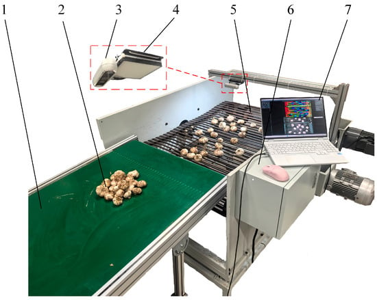
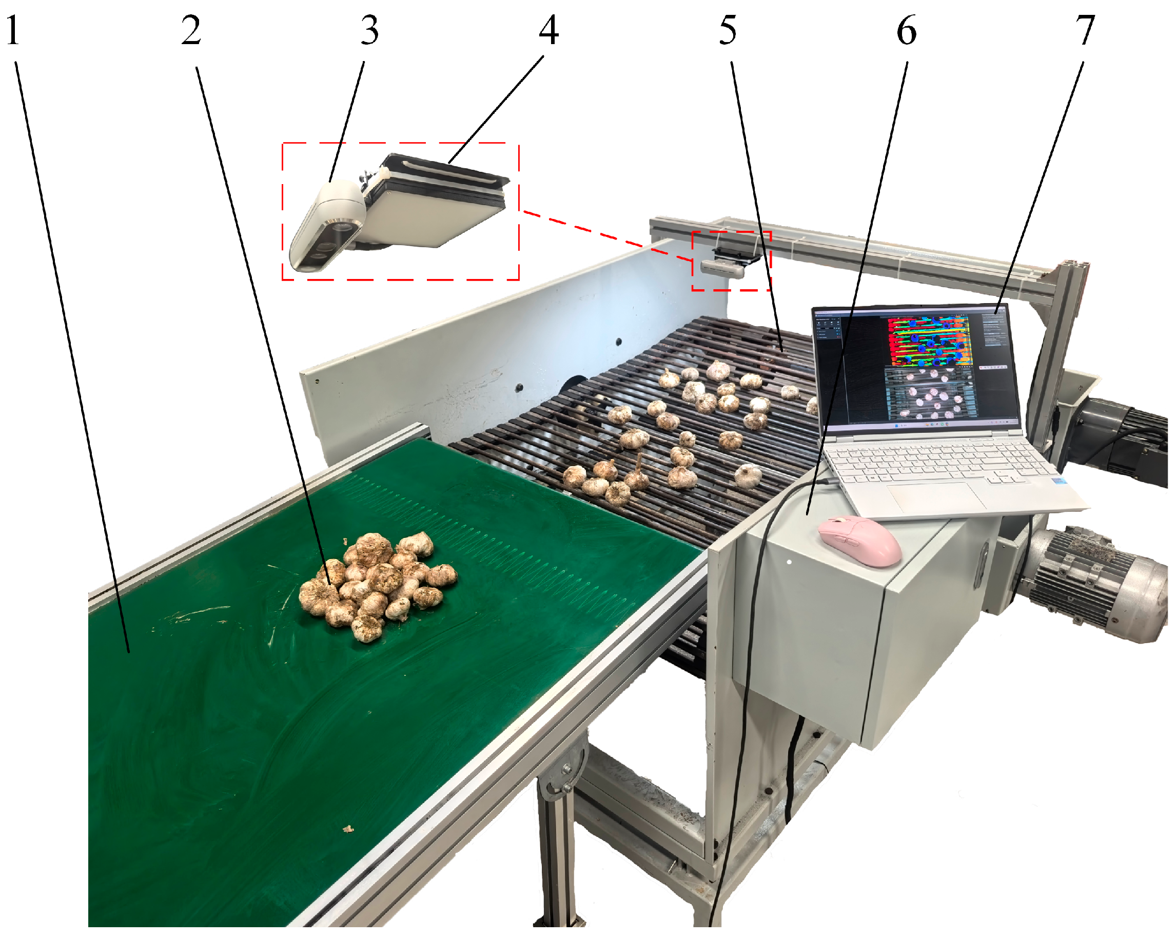
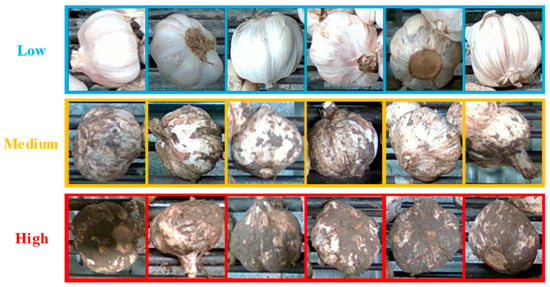
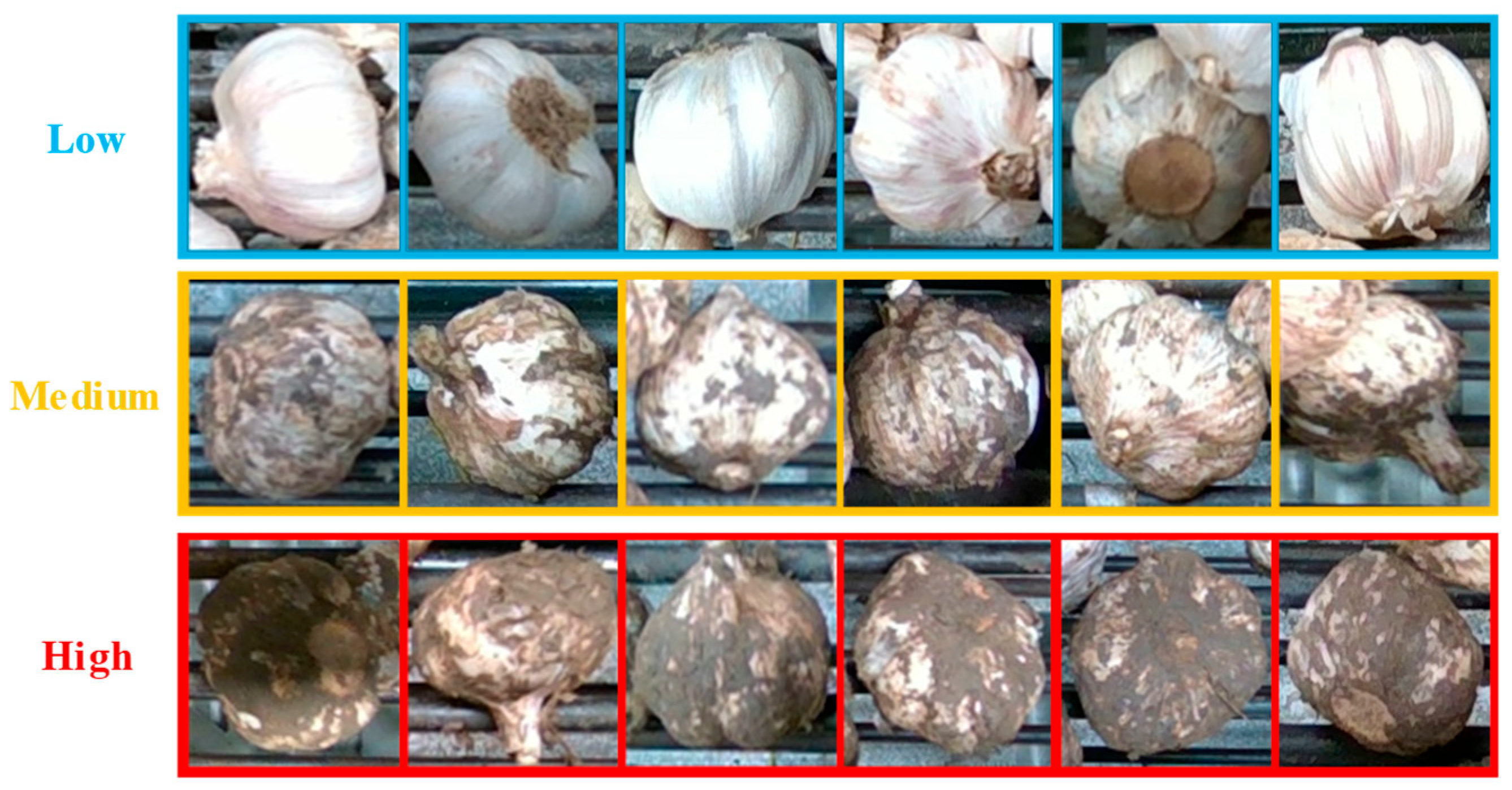
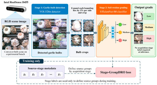
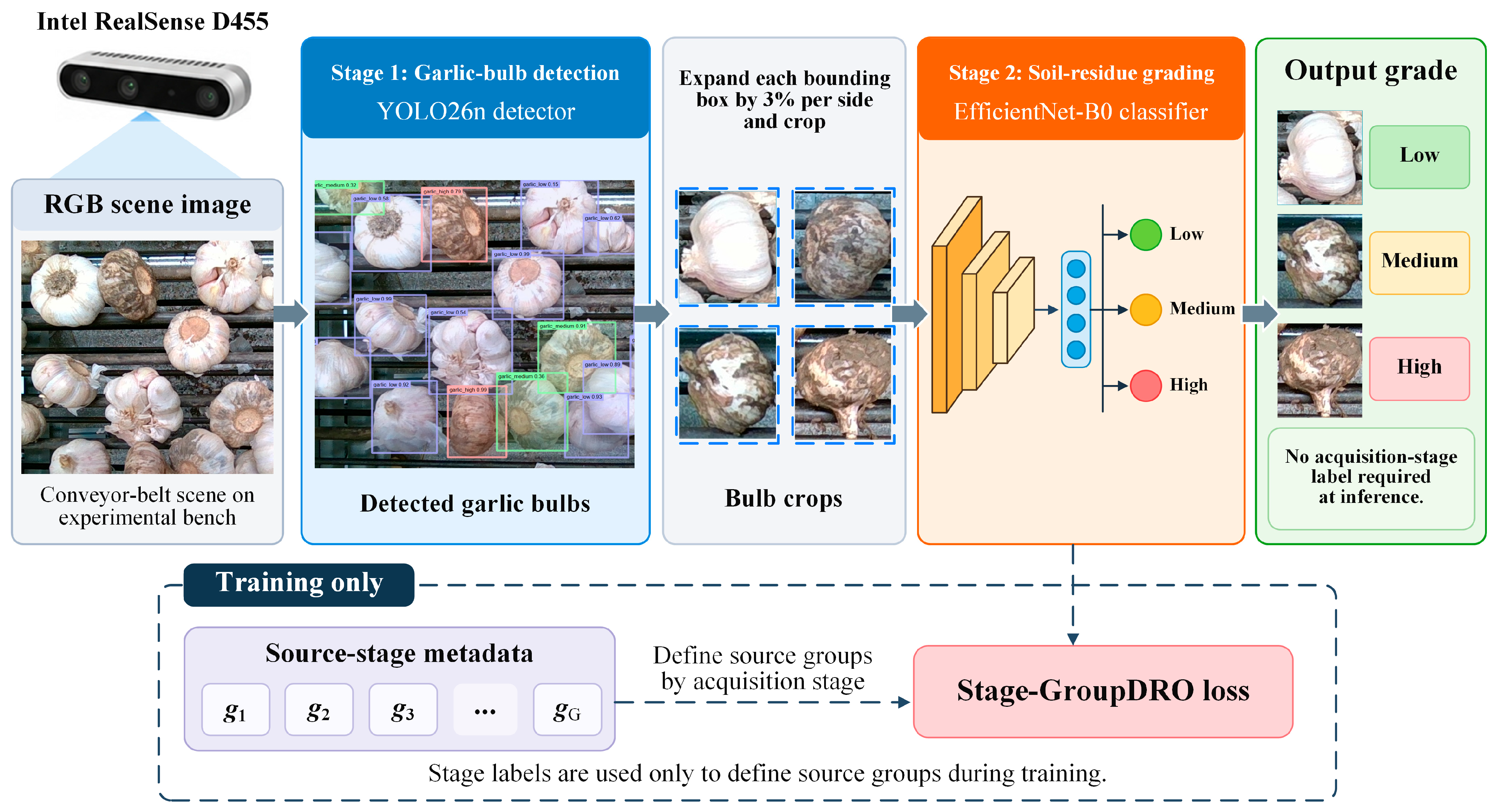
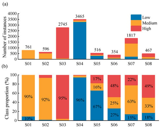
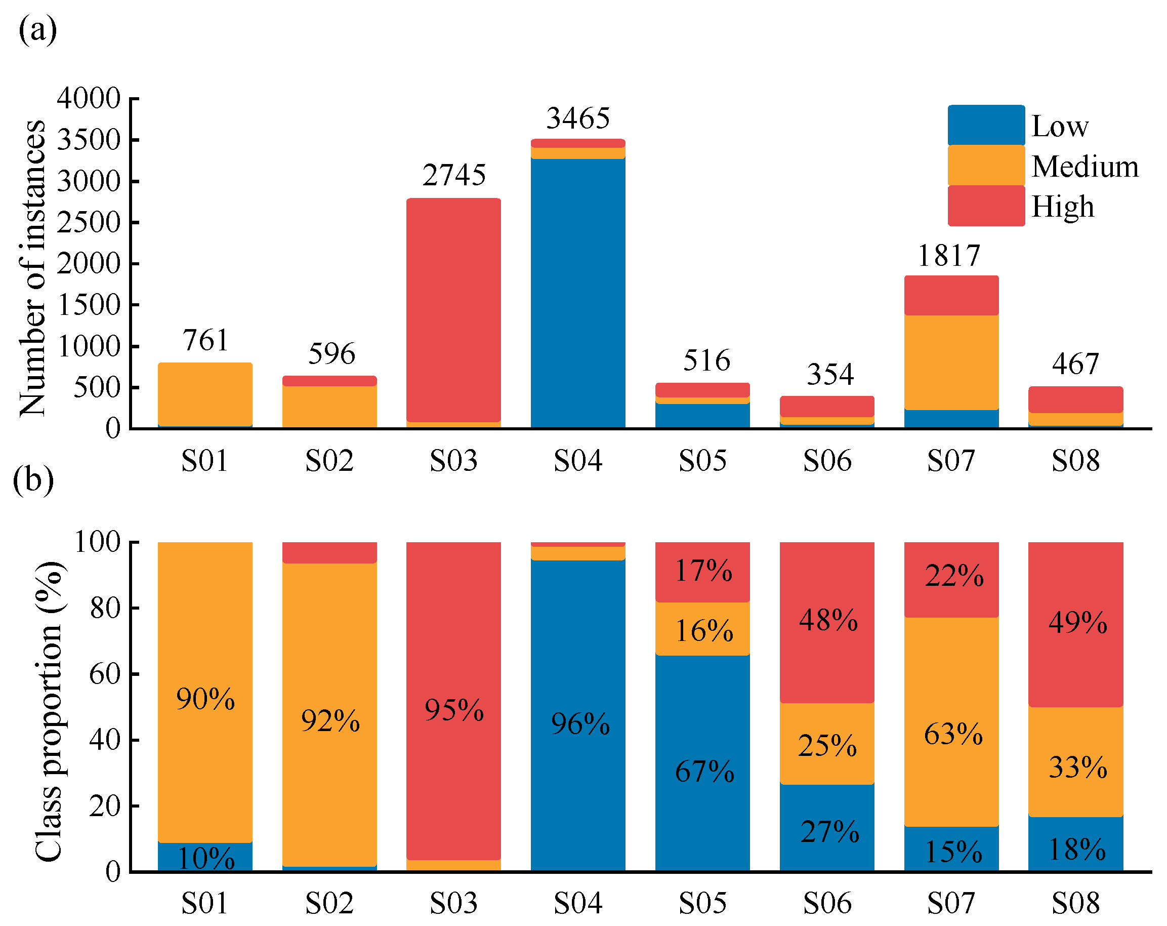
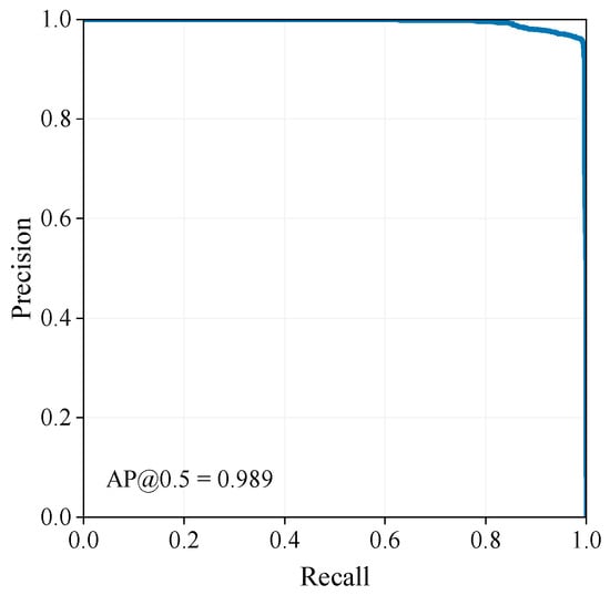
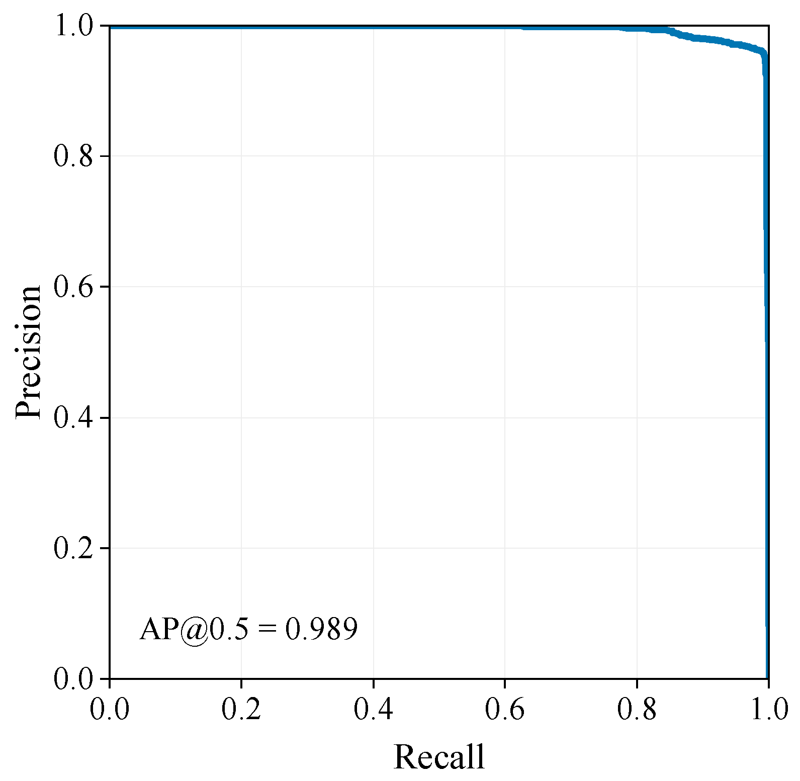
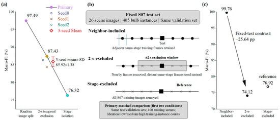
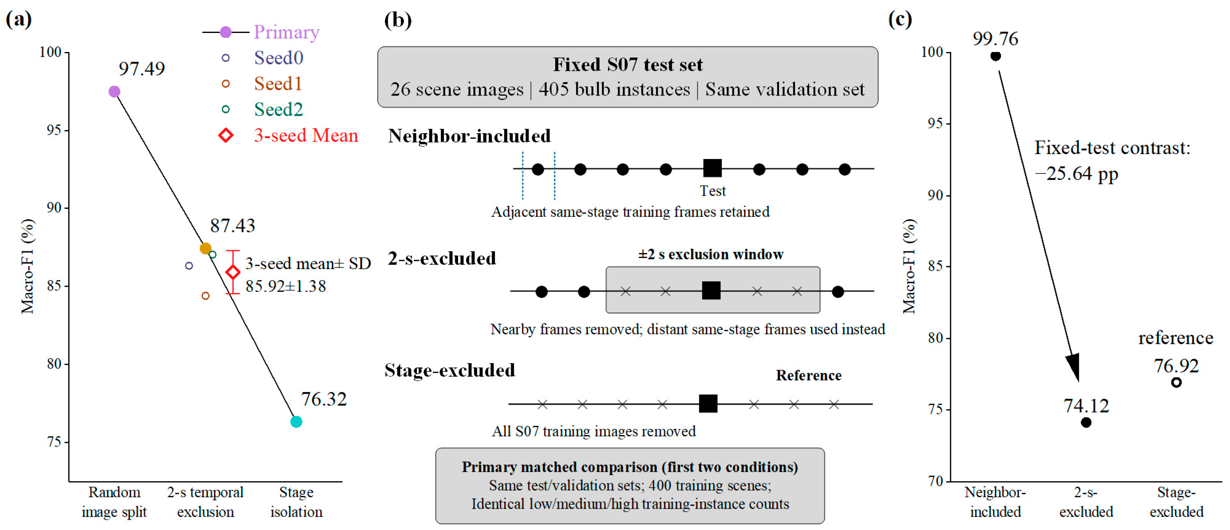
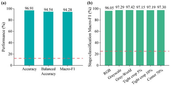
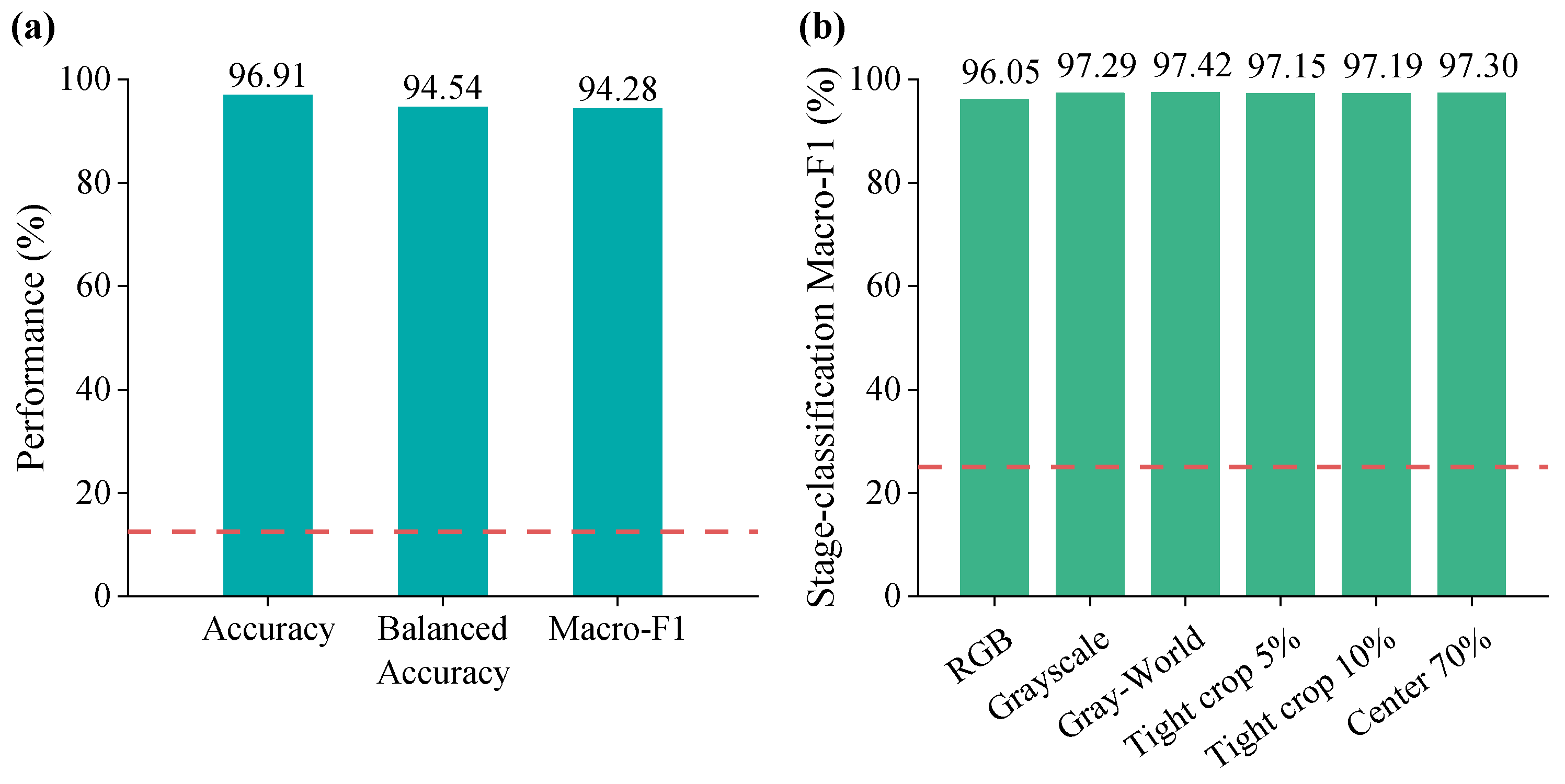
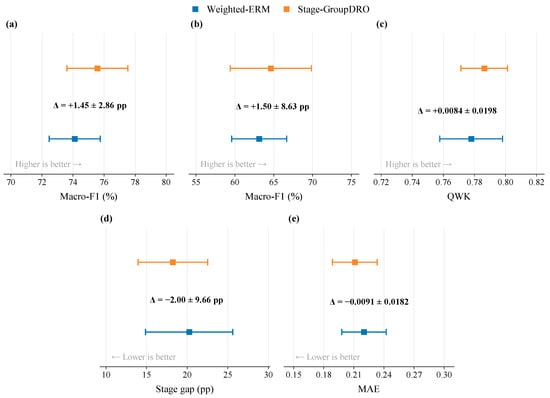
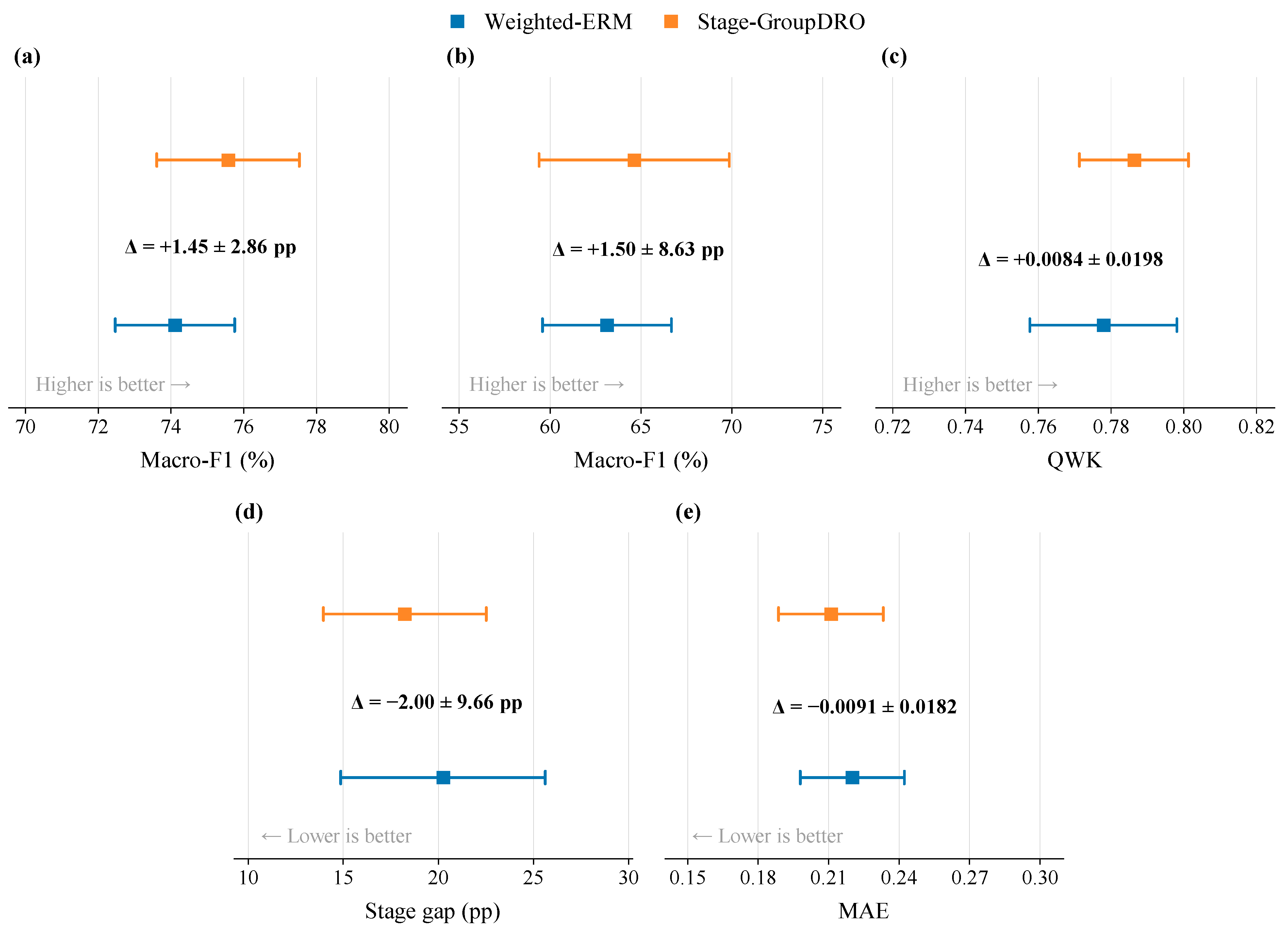
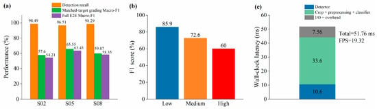

Disclaimer/Publisher’s Note: The statements, opinions and data contained in all publications are solely those of the individual author(s) and contributor(s) and not of MDPI and/or the editor(s). MDPI and/or the editor(s) disclaim responsibility for any injury to people or property resulting from any ideas, methods, instructions or products referred to in the content. |
© 2026 by the authors. Licensee MDPI, Basel, Switzerland. This article is an open access article distributed under the terms and conditions of the Creative Commons Attribution (CC BY) license.