


Abstract
Conventional agricultural productivity assessments that exclude carbon emissions may provide an incomplete representation of environmental performance, particularly when production technologies differ across regions. This study examines how excluding agricultural carbon emissions changes measured productivity growth in Chinese agriculture. Using panel data for 30 provinces from 2012 to 2021, we apply a Global Malmquist–Luenberger (GML) framework using regional group frontiers and a national meta-frontier. Productivity is estimated with and without carbon emissions and decomposed into efficiency change (EFFCH) and global technology-gap change (GTC). Regional technology gap ratios (TGRs) are also examined. Under constant returns to scale, the mean group-frontier GML index increases from 1.011 to 1.012 when emissions are excluded, while the meta-frontier index rises from 1.014 to 1.025. However, the direction of the difference varies across provinces and years. Under the meta-frontier, excluding emissions increases mean EFFCH but reduces mean GTC. The Central region records a lower emissions-inclusive TGR than the Eastern and Western regions, indicating a larger measured technology gap. Sensitivity analyses using variable returns to scale, alternative input specifications, and leave-one-province-out estimation show that some differences depend on modeling choices. These results demonstrate the importance of environmental specification and reference technology in interpreting agricultural productivity growth.
1. Introduction
With the accelerating pace of global climate change, green growth has emerged as a central pillar of sustainable development strategies worldwide. In the agricultural sector, green growth extends beyond the expansion of output and income to encompass environmental protection, resource efficiency, and long-term ecological sustainability [1]. In China, green agricultural development has been explicitly positioned as a key component of supply-side structural reform and high-quality agricultural modernization [2]. Over the past decades, agricultural development has played a crucial role in ensuring food security and supporting rural economic growth [3,4]. However, conventional productivity measures are not necessarily environmentally neutral. When carbon emissions are excluded from productivity measurement, environmental costs are not incorporated into the production technology, potentially affecting estimated agricultural productivity growth and the interpretation of its components [5].
Anthropogenic activities remain the dominant driver of global carbon dioxide emissions [6]. As one of the world’s largest carbon emitters, China has committed to peaking carbon emissions before 2030 and achieving carbon neutrality before 2060 [7]. Agriculture contributes to China’s carbon emissions, accounting for approximately 7% of the national total, while traditional input-intensive agricultural practices have placed considerable pressure on the ecological environment [8]. Consequently, improving agricultural green production efficiency has become an important pathway toward sustainable agricultural development [9]. Nevertheless, China’s agricultural sector made limited progress in reducing greenhouse gas emissions during 2008–2017 [10]. These environmental challenges highlight the importance of incorporating environmental considerations into agricultural productivity assessment. Conventional productivity measures that exclude undesirable outputs may provide an incomplete assessment of agricultural performance because environmental outcomes are not explicitly represented in production technology [8].
Previous studies have incorporated carbon emissions and other undesirable outputs into productivity measurement to evaluate agricultural green performance [6,9,11,12,13]. Several studies have identified technological change as an important contributor to agricultural green productivity growth, while also documenting regional differences [8,14,15]. Related research has examined the influence and spatial spillover effects of carbon emissions trading on agricultural green total factor productivity [16]. However, the present study focuses on a different measurement question: how does excluding agricultural carbon emissions change estimated productivity growth and its components when provinces are evaluated against alternative reference technologies?
2. Theoretical Framework
2.1. Environmental Constraints and Productivity Measurement
The methodological development of environmentally adjusted productivity measurement provides a basis for addressing this issue. The directional distance function was introduced to accommodate simultaneous adjustments in desirable and undesirable outputs [17]. Building on this framework, Chung et al. [18] developed the Malmquist–Luenberger (ML) productivity index, enabling intertemporal productivity comparisons while explicitly incorporating undesirable outputs. Although the ML index represents an important methodological advance, subsequent research has identified several limitations of conventional ML formulations, including intertemporal infeasibility and difficulties in ensuring comparability across periods. In response, Oh [19] introduced the Global Malmquist–Luenberger (GML) index using a global production possibility set, thereby establishing a common intertemporal reference technology and addressing the infeasibility problem associated with conventional ML formulations. Zhang and Choi [20] further developed a meta-frontier non-radial Malmquist index incorporating slack adjustments, while Emrouznejad and Yang [21] proposed a RAM-based global Malmquist–Luenberger framework that allows non-proportional efficiency adjustments. These methodological developments have expanded the flexibility of productivity measurement under environmental constraints.
The application literature further demonstrates that environmental adjustment can affect both productivity estimates and their decomposition. ML- and GML-based measures have been applied to environmentally intensive industries, including manufacturing and energy production. Existing evidence indicates that incorporating undesirable outputs can alter productivity estimates and the decomposition of productivity growth [22,23]. Kumar [24] found that environmental adjustment affects estimates of technical and efficiency change. Using a Malmquist–Luenberger productivity framework for U.S. agriculture, Kim and Kim [25] found that excluding undesirable outputs led to an overestimation of annual productivity growth. Their findings highlight the importance of environmental adjustment in agricultural productivity measurement, although the direction and magnitude of such differences may vary across empirical settings and reference technologies. Yu et al. [26] further assessed eco-efficiency and productivity growth in China’s pulp and paper industry while accounting for undesirable environmental outputs.
More recent studies have continued to develop environmentally adjusted productivity frameworks. Zhu et al. [6], for example, developed a total factor carbon emission productivity framework linking energy inputs and carbon emissions within a GML framework and found that productivity dynamics were primarily driven by technological change rather than efficiency change. Wei et al. [23] examined carbon productivity dynamics and their drivers in China’s thermal power sector. Collectively, these studies demonstrate the importance of incorporating environmental considerations into productivity assessment, while also indicating that environmental adjustment can influence the interpretation of technological and efficiency changes.
Agricultural studies have further highlighted the importance of environmental considerations in productivity assessment. Zhang et al. [27] identified regional differences in agricultural carbon emission efficiency, while Wu et al. [28] examined agricultural ecological efficiency under low-carbon policy interventions. Yang et al. [29] incorporated undesirable outputs into agricultural green productivity measurement. Although these studies provide valuable evidence on environmentally adjusted agricultural performance, they do not directly establish how environmental-specification differences vary across alternative reference technologies. This distinction motivates a joint consideration of environmental specification and regional technological heterogeneity.
2.2. Technological Heterogeneity and Meta-Frontier Approaches
Environmental specification is only one dimension of agricultural productivity measurement; the choice of reference technology is another. Agricultural production conditions vary across regions because of differences in agroecological conditions, factor endowments, and technology adoption. Meta-frontier approaches account for such heterogeneity by distinguishing group-specific production technologies from a broader reference technology. In China, Zhong et al. [30] documented regional differences in technical efficiency, production potential, and technology gaps, while Wang and Du [31] examined the relevance of heterogeneous production technologies for agricultural green productivity measurement. Zhong et al. [32] further investigated regional and scale heterogeneity in pig production using a three-level meta-frontier framework. These studies establish the importance of accounting for technological heterogeneity. However, identifying regional technology gaps does not, by itself, reveal whether the measured consequences of excluding undesirable outputs differ between group-frontier and meta-frontier specifications. Table 1 summarizes the methodological developments and empirical findings discussed above.
Table 1.
Summary of key studies on environmentally adjusted productivity measurement and agricultural green productivity.
2.3. Conceptual Framework and Research Gap
Previous research has established important foundations for environmentally adjusted productivity measurement and the analysis of heterogeneous production technologies. Studies based on directional distance functions and ML or GML indices have developed methods for incorporating undesirable outputs into productivity assessment [17,18,19,20,21]. Empirical research has also shown that excluding undesirable outputs can alter measured productivity growth, including in agricultural applications [24,25]. Separately, meta-frontier studies have documented technological differences across agricultural regions and production systems [30,31,32]. These contributions establish the relevance of environmental adjustment and technological heterogeneity, but they address distinct dimensions of productivity measurement.
Three related issues motivate the present study. First, the direction and magnitude of environmental-specification differences may depend on whether observations are evaluated against regional group-frontiers or a national meta-frontier. Second, differences in aggregate productivity growth may conceal contrasting changes in efficiency change and global technology-gap change. Third, the interpretation of these differences requires assessing their sensitivity to returns-to-scale assumptions, input selection, and the composition of the provincial sample. These issues are particularly relevant when small average differences are used to draw conclusions about environmental omissions.
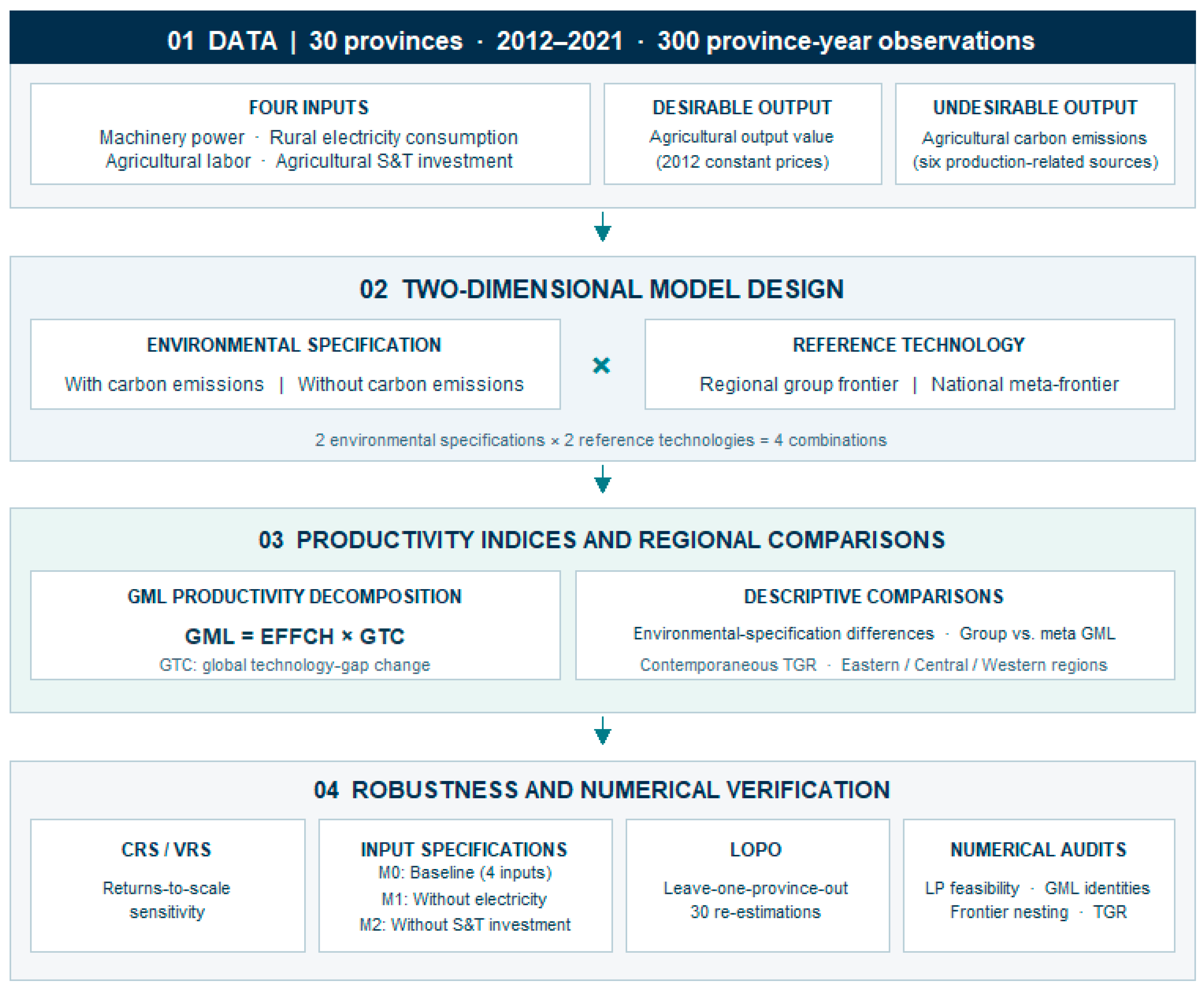
To examine these issues, this study applies a Global Malmquist–Luenberger (GML) framework to a balanced panel of 30 Chinese provinces from 2012 to 2021. Productivity is estimated with and without agricultural carbon emissions under regional group-frontiers and a national meta-frontier. The analysis compares aggregate GML productivity growth and its efficiency-change (EFFCH) and global technology-gap change (GTC) components. Contemporaneous technology gap ratios (TGRs) are examined separately to characterize regional technological heterogeneity. CRS/VRS comparisons, alternative input specifications, and leave-one-province-out analyses are used to assess the sensitivity of the results. The overall analytical framework is illustrated in Figure 1.
This study contributes to the literature in three ways. First, it extends empirical comparisons of environmentally adjusted productivity by examining how environmental-specification differences vary across regional group-frontiers and a national meta-frontier. Second, it distinguishes changes in aggregate GML productivity from changes in efficiency change (EFFCH) and global technology-gap change (GTC), while separately examining contemporaneous technology gap ratios (TGRs) to characterize regional technological heterogeneity. Third, it assesses the sensitivity of environmental-specification differences to returns-to-scale assumptions, input selection, and provincial sample composition, identifying both relatively stable patterns and results that require more cautious interpretation. Together, these contributions provide a more nuanced understanding of how measured agricultural productivity growth varies across environmental specifications and reference technologies.
Figure 1.
Analytical framework for assessing environmental-specification differences and technological heterogeneity in Chinese agricultural productivity. Notes: The framework combines two environmental specifications (with and without agricultural carbon emissions) and two reference technologies (regional group-frontier and national meta-frontier). GML denotes the global Malmquist–Luenberger productivity index, EFFCH denotes efficiency change, GTC denotes global technology-gap change, and TGR denotes the contemporaneous technology gap ratio. CRS and VRS represent constant and variable returns to scale, respectively. S&T denotes science and technology, and LOPO denotes leave-one-province-out analysis.
3. Methodology
3.1. Analytical Framework
This study examines whether excluding agricultural carbon emissions changes measured productivity growth in Chinese agriculture. It combines directional distance functions (DDFs), the Global Malmquist–Luenberger (GML) index, and a meta-frontier framework. The approach accommodates undesirable outputs and allows regional technologies to differ [18,19,33].
Two specifications are estimated using identical inputs, desirable outputs, observations, and reference-period structures. The environmental specification includes agricultural carbon emissions as an undesirable output; the alternative omits emissions. Separate group frontiers are estimated for Eastern, Central, and Western China, and a national meta-frontier is constructed from all 30 provinces [34]. The global reference set pools observations over 2012–2021, providing a fixed benchmark across years [18,35]. CRS is the benchmark and VRS is examined as a sensitivity specification.
3.2. Production Technology and Directional Distance Function
3.2.1. Environmental Production Technology
Let be the input vector for province i in year t, yit ∈ R+ desirable agricultural output, and bit ∈ R+ agricultural carbon emissions. Inputs are agricultural machinery power, rural electricity consumption, agricultural labor, and agricultural science and technology investment. Environmental production technology is defined as follows:
PE(x) = {(y,b):x can produce (y,b)}
For a reference set R containing nR observations, the empirical DEA technology is
Here, XR, YR, and BR are reference input, desirable-output, and undesirable-output matrices, and λ is the vector of intensity weights. The equality restriction on undesirable output prevents emissions from being treated as freely removable within the specified DEA representation. It is a modeling choice, not by itself proof that every weak-disposability or null-jointness axiom holds; this distinction is particularly important for VRS technologies [36,37].
CRS imposes nonnegative intensity weights. Under VRS the additional convexity restriction is
The no-emissions specification removes the undesirable output restriction:
The VRS convexity condition is also applied to this specification when required.
3.2.2. Directional Distance Function
The DDF evaluates the feasible proportional expansion of desirable output and contraction of undesirable output, conditional on inputs [18]. The chosen direction is g = (yit,−bit). For environmental technology,
subject to
XRλ ≤ xit,
YRλ ≥ (1 + β)yit,
BRλ = (1 − β)bit,
λ ≥ 0,
β ≥ 0.
For the non-emissions technology, the corresponding program is
subject to
XRλ ≤ xit,
YRλ ≥ (1 + β)yit,
λ ≥ 0,
β ≥ 0.
For VRS, is additionally imposed. The optimum β measures the greatest feasible improvement along the selected direction; a value of zero is a valid optimum. All linear programs are solved with Rglpk. The constraints are normalized by the strictly positive values of the evaluated observation, and computed solutions are checked for optimal status and numerical feasibility.
3.3. Group and Meta-Frontier Global Malmquist–Luenberger Indices
3.3.1. Global Reference Technologies
Global reference technologies are formed by pooling observed production activities over 2012–2021. Let denote the observations in region r in year t. The regional global technology is
and the national meta-frontier is
Here, s ∈ {E,N} identifies the emissions and no-emissions technologies, respectively. The national pool contains every regional observation, so its feasible technology nests each regional technology under a common returns-to-scale and environmental specification. This implements the distinction between group-specific and common reference technologies in meta-frontier analysis [33,34]. The global pooling approach is consistent with the global productivity measurement framework developed in previous studies [19,35].
3.3.2. Group GML and Meta-Frontier GML
For province i in region r, the group index is
The national meta-frontier index is
Both indices use a fixed global reference technology. Values above one indicate measured productivity improvement, whereas values below one indicate deterioration. Group GML evaluates change relative to regional global technology, whereas MFGML uses pooled national technology. The indices are computed separately with and without carbon emissions and under CRS and VRS.
3.3.3. Efficiency Change and Global Technology-Gap Change
The contemporaneous efficiency-change factor is
where F ∈ {Group,Meta}. The ratio between the global and contemporaneous distances is
The intertemporal change in this ratio is
These definitions yield the exact identity
The residual component is denoted as TECH_RATIO in the R implementation and is interpreted here as global technology-gap change (GTC). This component should not be interpreted as conventional adjacent-period Malmquist–Luenberger technical change, because it is derived from changes in the global-to-contemporaneous technology-gap ratio rather than directly measuring shifts in the production frontier. This distinction is important for avoiding unwarranted frontier-shift interpretation.
3.4. Measurement of Environmental-Specification Differences
The emissions specification evaluates productivity change subject to a carbon-emissions constraint, while the no-emissions specification removes that constraint. The meta-frontier difference is
and the group-frontier difference is
Component differences are likewise defined as
Positive values indicate higher estimated indices when emissions are excluded; negative values indicate the reverse. No sign restriction is imposed. Although removing the emissions constraint expands the feasible production set for a given observation, the sign of a productivity change difference is not predetermined because each index is a ratio of intertemporal distances. The resulting differences are interpreted as specification sensitivity rather than independently identified causal bias.
3.5. Environmental Omission and Technological Heterogeneity
The meta-frontier framework allows for technological heterogeneity across groups [33,34]. To distinguish environmental-specification sensitivity from differences arising from the choice of technology reference, the study defines the following descriptive measures:
This difference captures variation in measured productivity change associated with the choice of reference technology. It should not be interpreted as the absolute distance between regional and national production frontiers or as a direct measure of the technology gap.
To characterize contemporaneous technological heterogeneity, we additionally calculate the technology gap ratio (TGR):
where and denote directional distance functions evaluated relative to the regional group technology and the national meta-frontier, respectively, under specification s. Given the nesting of regional production technologies within the national meta-frontier, a TGR closer to unity indicates a smaller measured technology gap, while a lower value indicates a larger gap. This interpretation is conditional on the adopted directional-distance formulation and the corresponding frontier construction.
The empirical analysis compares environmental-specification differences under group-frontier and meta-frontier technologies and examines contemporaneous technology gap ratios across the Eastern, Central, and Western regions. These measures provide complementary descriptive perspectives on productivity measurement and regional technological heterogeneity. The analysis is descriptive and does not seek to establish causal relationships or statistically significant associations between environmental-specification differences and meta-frontier adjustments.
3.6. Data and Sensitivity Analysis
3.6.1. Data and Deflation
The balanced panel comprises 30 mainland Chinese provinces over 2012–2021, excluding Tibet because of data limitations. It contains 300 province-year observations and yields 270 consecutive-year productivity-change observations. Four inputs are included: agricultural machinery power (x1), rural electricity use (x2), agricultural labor (x3), and agricultural science and technology investment (x4). Agricultural production value is the desirable output (y), and agricultural carbon emissions are the undesirable output (b). Total crop-sown area (x5) was used as an additional proxy for agricultural land input in the M3 sensitivity specification.
The statistical data were obtained from the China Statistical Yearbook and the China Rural Statistical Yearbook, published by the National Bureau of Statistics of China (https://www.stats.gov.cn/), together with the compiled datasets described below. The agricultural carbon emissions data and their accounting method are described in Section 3.6.2.
Rural electricity use (x2) is measured using the statistical indicator “Rural Electricity Consumption”. This indicator is used as a proxy for electricity-related input in the rural production environment. Because rural electricity consumption is not necessarily restricted to agricultural production, it may also capture electricity use in non-agricultural activities.
Agricultural science and technology investment (x4) was obtained from a third-party compiled dataset made available on 29 June 2023 through a Baidu Netdisk collection titled “Agricultural Carbon Emissions, Agricultural Statistical Yearbooks, Rural Revitalization, Micro-level Surveys, and Other Agriculture, Rural Areas, and Farmers Research Datasets” (https://pan.baidu.com/s/1yOviOVc8E9lfxbP63CXMvg; accessed on 30 May 2025). In this study, x4 is used as a proxy for financial resources associated with agricultural scientific and technological activities, rather than as a direct measure of agricultural R&D expenditure. As the underlying compilation methodology is not fully documented in the available source materials, the variable is interpreted within this operational definition.
The contemporaneous inclusion of x4 in the DEA framework reflects resources recorded in each observation year, while the productivity effects of such investment may emerge over a longer period. To assess the sensitivity of the estimates to this input specification, Model M2 excludes x4 and re-estimates the productivity indices under both CRS and VRS within the group- and meta-frontier frameworks. This alternative specification provides an additional basis for evaluating the dependence of the reported results on the inclusion of the compiled investment proxy.
Agricultural science and technology investment and agricultural production value were converted to constant 2012 prices using the consumer price index (CPI) and an agricultural producer price index, respectively:
The CPI and agricultural producer price index data were obtained from the China Statistical Yearbook, published by the National Bureau of Statistics of China (https://www.stats.gov.cn/; accessed on 12 October 2026). The CPI was used to deflate nominal agricultural science and technology investment (x4), while the agricultural producer price index was used to deflate nominal agricultural production value (y). Both indices were expressed with 2012 as the base year (2012 = 100) before deflation.
The CPI was used as a proxy deflator for agricultural science and technology investment because a dedicated price index was unavailable. However, it may not fully reflect changes in the costs of agricultural science and technology inputs, potentially introducing measurement uncertainty into the productivity estimates.
Regional and national GML averages and their decomposition components are calculated as unweighted arithmetic means of province-period observations (270 observations nationally), without weighting by agricultural production value.
3.6.2. Agricultural Carbon Emissions
Agricultural carbon emissions were obtained from an existing provincial dataset constructed using an activity-based emission-factor approach. The dataset, entitled Agricultural Carbon Emissions Data for 31 Chinese Provinces, 2000–2021 (Including Calculation Procedures), was accessed through a Baidu Netdisk share in the Chinese Agriculture, Rural Areas and Farmers Research Data Collection (https://pan.baidu.com/s/1yOviOVc8E9lfxbP63CXMvg accessed on 30 May 2025), shared on 29 June 2023 [38]. This accounting approach is broadly consistent with the emission-factor methodology described in the 2006 IPCC Guidelines for National Greenhouse Gas Inventories [39] and has been applied in previous studies of agricultural carbon emissions [40,41,42].
The dataset covers six agricultural production-related emission sources: chemical fertilizers, pesticides, agricultural plastic film, diesel fuel, land tillage, and irrigation. The corresponding activity data, including fertilizer consumption, pesticide consumption, agricultural plastic film consumption, agricultural diesel consumption, total crop-sown area, and effective irrigation area, were originally compiled from the China Statistical Yearbook and the China Rural Statistical Yearbook and made available through the third-party dataset. Source-specific carbon emission coefficients were applied to these activity data to calculate agricultural carbon emissions. The underlying emissions accounting is expressed as follows:
where Cit denotes total agricultural carbon emissions in province i and year t, Akit is the activity level of emission source k, and EFk is its corresponding emission coefficient. The emission sources, activity measures, emission coefficients, and associated units documented in the source dataset are summarized in Supplementary Table S1.
The emission coefficients applied in the source dataset are 0.89 for chemical fertilizers, 4.93 for pesticides, 5.18 for agricultural plastic film, 0.59 for diesel fuel, 312.60 for land tillage, and 266.48 for irrigation. The coefficients for chemical fertilizers, pesticides, agricultural plastic film, and diesel fuel are closely aligned with those reported by Wen et al. [43], while the coefficients for land tillage and irrigation are consistent with those documented by Yao et al. [44]. Published studies provide further support for interpreting these coefficients on a carbon-mass basis. In particular, Luo et al. [45] explicitly report the coefficients for chemical fertilizers, pesticides, agricultural plastic film, diesel fuel, and irrigation in kg C per corresponding activity unit, while Wang et al. [46] report the land-tillage coefficient in kg C/km2.
The calculation workbook applies unit conversions before aggregating emissions from the six sources. Fertilizer and diesel consumption are recorded in 104 tonnes, pesticide and plastic film consumption in tonnes, and crop-sown and effective irrigation areas in 103 hectares. For land tillage, 103 hectares are converted into square kilometers to match the coefficient of 312.60 kg C/km2. For irrigation, 103 hectares are converted into hectares to match the coefficient of 266.48 kg C/ha. All six emission components are then expressed in 104 tonnes of carbon before aggregation. The corresponding conversion formulas are provided in Supplementary Table S1, with crop-sown area used as a proxy for tillage activity.
The emission coefficients are consistent with a carbon-mass (C) accounting convention, as supported by the published literature and the unit conversions implemented in the calculation workbook. Accordingly, the aggregate agricultural carbon emissions are interpreted as 104 tonnes C rather than tonnes CO2 or CO2e. No additional conversion between C and CO2, or to CO2e, was applied in the present study.
The original dataset covers 31 Chinese provinces from 2000 to 2021. This study uses observations for 30 provinces during 2012–2021, excluding Tibet. The resulting emission values are incorporated as the undesirable output in the GML model. The accounting boundary is restricted to the six specified production-related sources and excludes emissions from livestock, rice cultivation, and agricultural soil processes.
3.6.3. Regional Classification
The Eastern group contains Beijing, Tianjin, Hebei, Liaoning, Shanghai, Jiangsu, Zhejiang, Fujian, Shandong, Guangdong, and Hainan (11 provinces). The Central group comprises Shanxi, Jilin, Heilongjiang, Anhui, Jiangxi, Henan, Hubei, and Hunan (8 provinces). The Western group comprises Inner Mongolia, Guangxi, Chongqing, Sichuan, Guizhou, Yunnan, Shaanxi, Gansu, Qinghai, Ningxia, and Xinjiang (11 provinces). Membership is held fixed throughout the sample.
3.6.4. Returns-to-Scale Sensitivity
CRS is adopted as the baseline specification. To assess sensitivity to returns-to-scale assumptions, the full estimation is repeated under VRS by imposing the convexity restriction specified in Equation (3), following the variable-returns-to-scale DEA framework [47]. Both environmental specifications and both frontier frameworks are re-estimated under VRS. Differences in the magnitude and direction of the estimated indices and their decomposition components are examined to assess sensitivity to the returns-to-scale assumption. The environmental interpretation of the undesirable-output equality under VRS requires particular care [36].
3.6.5. Numerical Verification and Computational Diagnostics
The computational procedure verifies panel completeness, province-year uniqueness, regional classification, input–output validity, and price-deflation consistency. Linear programming solutions are checked for optimality, feasibility, and constraint satisfaction. Additional diagnostics examine frontier-nesting relationships, the GML decomposition identity, and the admissible range of contemporaneous technology gap ratios. CRS and VRS estimates are compared to assess sensitivity to the returns-to-scale assumption.
The CRS results comprise 270 province-period transitions across 30 provinces and nine annual periods. All 28 mathematical audit checks were passed, with a maximum recorded numerical discrepancy of 5.39 × 10⁻¹⁶. No missing or non-finite index values or recorded LP failures were identified. Detailed results are provided in Supplementary Table S2. These checks support the internal computational consistency of the estimates but do not establish the validity of the underlying production technology assumptions. Moreover, as noted by Simar and Wilson [48], statistical inference in nonparametric frontier models requires procedures beyond numerical verification. In addition, 8640 DDF evaluations were independently re-solved under CRS and VRS, all of which passed the numerical comparison checks, with a maximum absolute difference of 1.08 × 10⁻¹⁴ between the original and independently obtained solutions.
3.6.6. Alternative Input Specifications and Frontier Discrimination
The selection of input and output variables is an important consideration in DEA applications because model dimensionality and variable specification may affect frontier discrimination and efficiency measurement [49]. To evaluate the sensitivity of the estimated productivity measures to input selection, four input specifications are considered.
The baseline model (M0) includes agricultural machinery power, rural electricity consumption, agricultural labor, and agricultural science and technology investment. Model M1 excludes rural electricity consumption, whereas Model M2 excludes agricultural science and technology investment. All directional distance functions, global productivity indices, and their decomposition components are re-estimated under each specification while maintaining the same sample, output variables, and regional classification. Model M3 extends the baseline specification by including total crop-sown area as a fifth input, measured in thousand hectares. The corresponding input vector is defined as , where x5,it represents total crop sown area. The additional input is incorporated into the existing DEA input constraints without changing the output variables, directional vector, sample period, or regional classification.
The sensitivity analyses are conducted under constant returns to scale (CRS) and variable returns to scale (VRS), separately for the group and meta-frontiers and for production technologies with and without undesirable outputs. For each specification, the environmental-specification difference in productivity growth is defined as
Here, m ∈ {M0, M1, M2, M3} denotes the input specification, r ∈ {CRS, VRS} represents the returns-to-scale assumption, and f ∈{Group, Meta} identifies the reference frontier. The subscripts i and t denote province i and the productivity transition from year t to year t + 1, respectively. An analogous environmental-specification difference is calculated for the global technology-gap-change component (GTC).
To assess consistency between the baseline and alternative models, Pearson correlation coefficients, sign-agreement rates, and changes in mean differences are calculated. The sign-agreement rate is expressed as
Here, S denotes the set of matched province-year transitions, N is the number of transitions in S, and 1 [1(ΔGMLᵢₜ(m,r,f) > 0) = 1{ΔGMLᵢₜ(M0,r,f) > 0}] denotes the indicator function, which equals one when the stated condition is satisfied and zero otherwise. The sign-agreement rate measures the percentage of observations for which the environmental-specification differences are classified consistently under the alternative and baseline input specifications. A difference is classified as positive if it is strictly greater than zero and as non-positive otherwise. No numerical tolerance is applied in this sign-agreement calculation; therefore, small positive differences remain positive, whereas zero and negative differences are classified as non-positive.
The discriminatory power of the contemporaneous regional DEA frontiers is evaluated by calculating the percentage of observations located on the efficient frontier:
Here, D denotes the directional distance function evaluated against the contemporaneous group frontier incorporating undesirable outputs, and Nᵍ is the total number of province-year observations in region g. Observations with directional distance no greater than 10−7 are classified as frontier-efficient. A high frontier share may indicate limited discrimination when the number of reference observations is small relative to the dimensionality of production technology.
3.6.7. Leave-One-Province-Out Sensitivity Analysis Procedure
DEA frontier estimates may be sensitive to influential observations, which can affect the shape of the estimated production possibility set [50]. For each exclusion, the directional distance functions, GML productivity indices, and their decomposition components are recalculated under both CRS and VRS, with and without undesirable outputs.
To ensure comparability, the LOPO estimates are matched with the corresponding full-sample baseline estimates for the same retained province-period observations. This matching procedure avoids conflating changes in the estimated frontier with changes in the composition of the observations being compared.
For each excluded province k, the change in the mean environmental-specification difference is defined as:
The mean absolute change in the environmental-specification difference is calculated as:
In these expressions, ρ denotes the set of 30 provinces, and N−k = 261 represents the number of retained province-period observations (29 provinces × 9 consecutive-year transitions). The term ΔGMLᵢₜ(−k,r,f) denotes the environmental-specification difference estimated after excluding province k, whereas ΔGMLᵢₜ(M0,r,f) is the corresponding full-sample baseline estimate.
4. Results and Discussion
4.1. Descriptive Statistics and Regional Characteristics
Table 2 presents the descriptive statistics for agricultural inputs and outputs across China’s Eastern, Central, and Western regions from 2012 to 2021. The sample covers 30 provinces and contains 300 province-year observations.
Table 2.
Descriptive statistics of agricultural production variables by region, 2012–2021.
The Central region recorded the highest average agricultural machinery power (5179.12), agricultural labor input (960.80), agricultural science and technology investment (585.78), and agricultural output value (2263.30). It also had the highest average carbon emissions (451.06). The Eastern region, by contrast, had the highest rural electricity consumption (564.19), compared with 151.29 in the Central region and 93.98 in the Western region. These figures indicate differences in the scale and composition of agricultural production across regions.
Variation was also observed within regions. In the Eastern region, for example, the standard deviation of agricultural machinery power (3685.36) exceeded its mean (3183.19), indicating considerable differences among province-year observations. Overall, the descriptive statistics show that agricultural production conditions are not uniform across the three regions. These differences provide useful background for the subsequent group-frontier and meta-frontier analyses, although they do not, by themselves, establish differences in productive efficiency.
4.2. Agricultural Productivity Growth Under Group and Meta-Frontiers
Table 3 reports agricultural productivity growth across the three regions under the CRS assumption, with carbon emissions included as an undesirable output.
Table 3.
Regional agricultural productivity growth under CRS, with undesirable output, 2012–2021.
Under the group-frontier, the national mean GML index was 1.011. The Eastern region recorded the highest value (1.016), followed by the Central (1.012) and Western (1.005) regions. Efficiency change remained close to unity across all three regions, while the GTC component exceeded unity.
The meta-frontier results show a different regional ranking. The Eastern region again had the highest GML index (1.024), followed by the Western (1.012) and Central (1.004) regions. The national mean EFFCH index was 0.993, while GTC averaged 1.022. This suggests that the positive average GML change was accompanied by a decline in measured efficiency relative to the contemporaneous meta-frontier.
The differences between the two sets of estimates indicate that the choice of reference technology affects the measured pattern of agricultural productivity growth, particularly in the Central and Western regions.
4.3. Environmental Omission and Productivity Measurement
4.3.1. Environmental-Specification Differences Under the Group-Frontier
Table 4 compares provincial agricultural productivity indices under the group-frontier, with and without agricultural carbon emissions.
Table 4.
Provincial agricultural productivity indicators under CRS—Group-frontier.
At the national level, the mean GML index increased from 1.011 to 1.012 when carbon emissions were excluded. The mean EFFCH index also increased, from 0.999 to 1.006, whereas GTC decreased from 1.013 to 1.008. These results indicate that excluding carbon emissions slightly increased the measured productivity index, while EFFCH and GTC moved in opposite directions.
The results varied across provinces. In Jiangxi, the GML index increased from 1.037 to 1.114 when carbon emissions were excluded. A similar increase was observed in Shanxi, from 1.035 to 1.118. In contrast, the index declined from 1.005 to 0.975 in Anhui and from 0.998 to 0.958 in Jilin. These differences show that excluding carbon emissions does not systematically increase measured productivity growth in every province.
Overall, the group-frontier results indicate that agricultural productivity estimates are sensitive to the treatment of undesirable outputs. The direction and magnitude of this sensitivity differ across provinces and across the components of the GML index.
4.3.2. Environmental-Specification Differences Under the Meta-Frontier
Table 5 presents the corresponding results under the meta-frontier, which evaluates all provinces against a common national reference technology.
Table 5.
Provincial agricultural productivity indicators under CRS—Meta-frontier.
The mean GML index increased from 1.014 to 1.025 when carbon emissions were excluded. The mean EFFCH index rose from 0.993 to 1.016, while GTC declined from 1.022 to 1.010. The average difference in GML was therefore larger under the meta-frontier (0.011) than under the group-frontier (0.002).
Provincial results again showed considerable variation. Shandong recorded an increase in GML from 1.042 to 1.128, while Jiangxi increased from 1.019 to 1.073. By contrast, the index declined from 0.991 to 0.957 in Qinghai and from 0.993 to 0.963 in Jilin. These examples indicate that differences in estimated productivity between the two environmental specifications vary across provinces when evaluated against the national reference technology.
Compared with the group-frontier estimates, the meta-frontier results show a larger average difference between the two environmental specifications. This suggests that the choice of reference technology matters when assessing the sensitivity of agricultural productivity estimates to the inclusion of carbon emissions.
Figure 2 presents the spatial distribution of provincial GML indices under the group-frontier and meta-frontier specifications, with and without agricultural carbon emissions. The four maps use identical classification intervals to facilitate comparison across environmental specifications and reference technologies.
Figure 2.
Spatial distribution of provincial Global Malmquist–Luenberger productivity indices under alternative environmental specifications and reference technologies, 2012–2021.
Under the group-frontier, the national mean GML index increases slightly from 1.011 to 1.012 when carbon emissions are excluded. However, the provincial results show considerable variation. For example, the GML index increases from 1.037 to 1.114 in Jiangxi and from 1.038 to 1.118 in Shanxi, whereas it decreases from 1.005 to 0.976 in Anhui and from 0.998 to 0.958 in Jilin.
Under the meta-frontier, the national mean GML index rises from 1.014 to 1.025 following the exclusion of carbon emissions. This difference is larger than that observed under the group-frontier. The spatial distribution also changes more visibly, with the number of provinces recording GML values above 1.060 increasing from zero to five. Nevertheless, the direction of change remains heterogeneous. Shandong and Jiangxi record higher GML values when carbon emissions are excluded, while Qinghai and Jilin show lower values.
Overall, Figure 2 confirms that the treatment of undesirable outputs affects measured agricultural productivity growth, but the magnitude and direction of the differences vary across provinces. The larger average difference under the meta-frontier further indicates that the choice of reference technology is important when comparing alternative environmental specifications.
4.3.3. Decomposition of Environmental-Specification Differences
Table 6 examines how the differences in measured productivity growth are reflected in efficiency change (EFFCH) and the global technology-gap change. The results are based on 270 province–year observations under the CRS assumption.
Table 6.
Decomposition of environmental-specification differences in agricultural productivity growth (CRS, 2012–2021).
Under the group-frontier, excluding agricultural carbon emissions increases the mean GML index from 1.011 to 1.012. This relatively small difference conceals opposing movements in the two components. Mean EFFCH rises from 0.999 to 1.006, whereas mean GTC falls from 1.013 to 1.008. A similar pattern emerges under the meta-frontier, although the differences are larger. The mean GML index increases from 1.014 to 1.025, accompanied by an increase in EFFCH from 0.9925 to 1.0158 and a decline in GTC from 1.022 to 1.010.
The observation-level decomposition provides further detail. Under the group-frontier, the average EFFCH-related contribution to the GML difference is 0.0087, partly offset by a GTC-related contribution of −0.0071. Under the meta-frontier, the corresponding values are 0.0258 and −0.015. Thus, the positive differences in average GML arise from an EFFCH-related increase that exceeds the offsetting GTC-related decrease.
These averages, however, do not describe every province–year observation. Under the group-frontier, 125 observations have a positive GML difference, compared with 140 negative differences and five values close to zero. Under the meta-frontier, 139 differences are positive, 129 are negative, and two are close to zero. The direction of the measurement difference therefore varies substantially across observations.
Taken together, the results suggest that excluding carbon emissions changes not only the estimated productivity growth indices but also the relative contributions of their decomposition components. In this sample, the average GML difference is associated with an increase in the EFFCH component rather than an increase in GTC. The distinction is particularly important under the meta-frontier, where the two environmental specifications produce a larger difference in measured productivity growth.
To assess sensitivity to environmental specification, Table 7 summarizes the signed and absolute differences in GML and GTC across 270 province-period transitions under CRS, calculated as estimates without carbon emissions minus those with emissions. The results reveal heterogeneous differences across provinces and periods. The mean GML difference is positive under both the group-frontier (0.002) and meta-frontier (0.011), although positive differences account for only 46.30% and 51.48% of observations, respectively. In contrast, mean GTC differences are negative under both frontiers (−0.005 and −0.012). Mean absolute differences range from 0.039 to 0.046, indicating that positive and negative discrepancies partly offset each other in aggregate measures. These findings demonstrate sensitivity to environmental specification rather than systematic overestimation or statistical bias relative to a known true measure.
Table 7.
Distribution of environmental-specification differences in GML and GTC under CRS, 2012–2021.
4.3.4. Regional Technology Gaps Under Alternative Environmental Specifications
Table 8 presents regional technology gap ratios (TGRs) under alternative environmental specifications using the CRS framework. Unlike differences between group-frontier and meta-frontier GML indices, TGR measures the contemporaneous relative position of regional production technologies against the national meta-frontier. With carbon emissions included, the national mean TGR was 0.931 at period t and 0.925 at period t + 1. The Eastern and Western regions exhibited similar beginning-of-period TGR values (0.936), whereas the Central region recorded a lower value (0.916).
Table 8.
Regional technology gap ratios under alternative environmental specifications (CRS), 2012–2021.
When carbon emissions were excluded, the Eastern region exhibited the highest beginning-of-period TGR (0.846), followed by the Central (0.795) and Western (0.780) regions. Under the carbon-inclusive specification, the Central region also recorded the largest negative mean change in TGR (−0.015), compared with −0.001 in the Eastern region and −0.002 in the Western region. These findings indicate that measured regional technology gaps vary across environmental specifications and regions. However, the results are descriptive and do not establish statistically significant regional trends or causal relationships. Importantly, differences between group-frontier and meta-frontier GML indices should not be interpreted as contemporaneous technology gaps.
4.4. Temporal Dynamics
4.4.1. Temporal Dynamics of Group-Frontier GML
Table 9 and Figure 3 present the annual changes in group-frontier GML and its components under the two environmental specifications. The mean GML index was 1.011 with carbon emissions and 1.012 without them. Although the averages of the period were similar, the annual estimates differed noticeably in several years.
Table 9.
Temporal evolution of group-frontier GML and its components, 2012–2021.
Figure 3.
Temporal dynamics of group-frontier GML and its components under alternative environmental specifications.
With carbon emissions included, GML declined below unity in 2014–2015 (0.979) and 2018–2019 (0.970), before recovering to 1.053 in 2020–2021. Excluding carbon emissions produced a different pattern in some periods. The most pronounced difference occurred in 2019–2020, when GML was 1.000 with carbon emissions but only 0.927 without them. In contrast, the estimate for 2015–2016 increased from 1.005 to 1.046 when emissions were excluded. These differences indicate that the omission of undesirable outputs does not systematically raise the estimated productivity index.
The decomposition provides further insight into the annual variation. In 2019–2020, excluding carbon emissions reduced EFFCH from 0.979 to 0.945 and GTC from 1.022 to 0.986. Both components were higher under the specification without carbon emissions in 2020–2021. Figure 3 also shows that the movements of EFFCH and GTC were not always aligned, particularly during periods of declining GML.
The group-frontier estimates therefore reveal substantial year-to-year differences that are not apparent from the period averages alone. Although the two environmental specifications yield similar Mean GML estimates under the group-frontier, their annual productivity growth estimates differ in magnitude and, in some periods, direction.
4.4.2. Temporal Dynamics of Meta-Frontier GML
Table 10 and Figure 4 present the annual movements of meta-frontier GML and its components under the two environmental specifications. The mean GML index was 1.014 with carbon emissions and 1.025 without them, indicating a larger average difference than under the group-frontier.
Table 10.
Temporal evolution of meta-frontier GML and its components, 2012–2021.
Figure 4.
Temporal dynamics of meta-frontier GML and its components under alternative environmental specifications.
With carbon emissions included, GML fell below unity in 2014–2015 (0.995), 2018–2019 (0.980), and 2019–2020 (0.991). The corresponding estimates without carbon emissions were 0.988, 0.953, and 0.968. In 2020–2021, GML increased to 1.069 and 1.117, respectively, with the latter representing the highest annual estimate under either specification.
The decomposition reveals contrasting movements in EFFCH and GTC. In 2019–2020, excluding carbon emissions increased EFFCH from 1.007 to 1.029 but reduced GTC from 0.984 to 0.943. A similar pattern appeared in 2020–2021, when EFFCH increased from 0.986 to 1.083 while GTC decreased from 1.085 to 1.030. Thus, the higher GML estimate without carbon emissions in 2020–2021 was associated with a stronger efficiency-change component rather than a higher GTC.
These annual fluctuations may also reflect changing agricultural production conditions, including policy adjustments, weather disturbances, input cost fluctuations, and COVID-19-related disruptions. However, the GML framework does not identify their causal effects; these factors are therefore considered possible contextual influences rather than established explanations.
4.5. Robustness and Sensitivity Analyses
4.5.1. Robustness to Returns-to-Scale Assumptions
To assess sensitivity to returns-to-scale assumptions, the GML indices were re-estimated under variable returns to scale (VRS) using the same provincial sample, study period, and environmental specifications as the baseline constant returns to scale (CRS) model. Table 11 compares the resulting GML indices and their components.
Table 11.
Robustness of GML estimates and their components under CRS and VRS.
Under the group-frontier, mean GML with carbon emissions decreased from 1.011 under CRS to 1.007 under VRS, while the corresponding estimate without carbon emissions remained approximately 1.012. With carbon emissions included, EFFCH increased from 0.999 to 1.001, whereas GTC decreased from 1.013 to 1.006. Under the meta-frontier, GML decreased from 1.014 to 1.011 with carbon emissions and from 1.025 to 1.014 without them, indicating a smaller environmental-specification difference under VRS.
Overall, mean GML remained above unity across all specifications, although the magnitude of environmental-specification differences and the decomposition components varied with the returns-to-scale assumption. These findings suggest that the general pattern of measured productivity growth is retained under VRS, while the CRS estimates should be interpreted with consideration of scale sensitivity.
4.5.2. Sensitivity to Input Specification
Sensitivity to input selection was first assessed using two input-deletion models: M1 excludes rural electricity consumption, and M2 excludes agricultural science and technology investment. Both were compared with the four-input baseline model (M0), using the same provinces, study period, and environmental specifications.
As shown in Table 12, the mean GML difference between the specifications without and with carbon emissions remained positive across all input models under both CRS and VRS. Under CRS, the group-frontier difference increased from 0.002 in M0 to 0.009 in M1 and 0.007 in M2, while the corresponding meta-frontier differences were 0.011, 0.015, and 0.013. A similar pattern was observed under VRS, although the magnitudes varied.
Table 12.
Sensitivity of GML estimates to alternative input specifications.
The alternative input models nevertheless affected observation-level estimates. Across the eight comparisons involving M1 and M2 relative to the baseline model, correlations of province-period GML differences ranged from 0.770 to 0.904, with sign agreement ranging from 78.15% to 85.93%. Thus, the positive mean difference was retained, although its magnitude and observation-level distribution remained sensitive to input selection. The four-input model was retained as the baseline to provide broader coverage of agricultural production inputs.
To further assess the discriminatory power of the regional production frontiers, Supplementary Table S3 reports frontier membership based on contemporaneous group-frontier directional distance functions. Under CRS, the shares of frontier-efficient observations were 80.00%, 46.25%, and 50.00% in the Eastern, Central, and Western regions, respectively. Under VRS, these shares increased to 89.09%, 73.75%, and 76.36%. The relatively high frontier membership in the Eastern region, particularly under VRS, suggests limited discrimination among observations and warrants caution when interpreting regional productivity differences. Although the Central region has the smallest annual sample, it does not exhibit the highest frontier membership. These diagnostics complement the returns-to-scale and other sensitivity analyses but do not eliminate concerns about the dimensionality of regional DEA frontiers.
An additional sensitivity analysis was conducted by incorporating total crop-sown area as a fifth input (M3). Supplementary Table S4 reports the resulting GML indices and proportions of frontier-efficient observations under CRS and VRS. Under CRS, the average meta-frontier GML index incorporating carbon emissions remained nearly unchanged at 1.014 in both M0 and M3 when rounded to three decimal places. The corresponding index excluding carbon emissions declined from 1.025 to 1.021. Consequently, the mean environmental-specification difference decreased from 0.011 to 0.007, while remaining positive.
Under VRS, the mean meta-frontier environmental-specification difference decreased from 0.003 in M0 to 0.002 in M3. Thus, the average difference remained positive across all four meta-frontier configurations, although its magnitude was sensitive to input selection and returns-to-scale assumptions. The group-frontier results were less consistent, with the five-input CRS specification producing a slightly negative mean difference (−0.0001). These findings suggest that the direction of the average meta-frontier difference is relatively stable across the examined specifications, whereas its magnitude is model-dependent.
The inclusion of land was also associated with higher proportions of frontier-efficient observations. For the meta-frontier incorporating carbon emissions, the proportion increased from 27.0% to 34.3% under CRS and from 51.7% to 60.3% under VRS. Under the five-input VRS group-frontier specification, 83.7% of observations were frontier-efficient, reaching 92.7% in the Eastern region. These high proportions suggest reduced discriminatory power under more flexible DEA specifications, particularly for regional group-frontiers. The four-input CRS model is therefore retained as the baseline for consistency with the main analytical framework, while the land-augmented and VRS specifications are used to assess the sensitivity of the findings to alternative production technology assumptions.
4.5.3. Leave-One-Province-Out Sensitivity Analysis
A leave-one-province-out (LOPO) sensitivity analysis was conducted by excluding each of the 30 provinces in turn and re-estimating the production frontiers using the remaining 29 provinces. Each estimation contained 261 province-period observations, and the resulting environmental-specification differences were compared with matched baseline estimates.
As shown in Table 13, the mean absolute observation-level changes ranged from 0.001 to 0.002, with correlations ranging from 0.823 to 1.000 and sign agreement ranging from 85.1% to 100.0%. However, some exclusions affected the mean differences. Excluding Guizhou under the CRS group-frontier reversed the sign of the mean environmental-specification difference from 0.001 to −0.001.
Table 13.
Leave-one-province-out sensitivity of environmental specification differences.
Overall, the LOPO results suggest that observation-level patterns were largely preserved across most exclusions, although small mean differences remained sensitive to individual provinces. This sensitivity should be considered when interpreting the CRS group-frontier results.
4.6. Discussion
4.6.1. Environmental Omission and Agricultural Productivity Measurement
The results show that excluding agricultural carbon emissions affects productivity estimates, although the differences vary across reference technologies and periods. Under CRS, the mean group-frontier GML indices were 1.011 with emissions and 1.012 without them. The corresponding meta-frontier estimates were 1.014 and 1.025. The larger difference under the meta-frontier suggests that the choice of reference technology matters when evaluating environmental omissions.
Previous studies have shown the importance of incorporating undesirable outputs into productivity measurement. Chung et al. [18] introduced a directional distance function approach that accounts for desirable and undesirable outputs, while Oh [19] developed a global Malmquist–Luenberger index based on a common reference technology. Building on these approaches, the present study examines environmental omission under both regional and national production frontiers. Although previous research has documented higher productivity estimates when undesirable outputs are excluded in particular empirical settings, the present results indicate that this pattern does not hold uniformly across provinces, periods, and reference technologies.
The decomposition provides further evidence of this variation. Under the meta-frontier, excluding emissions increased mean EFFCH but reduced mean GTC. The latter represents changes in the relative distance between global and contemporaneous reference technologies, rather than an independent measure of technological innovation. Thus, changes in aggregate productivity estimates should not be interpreted as equivalent changes in technological progress.
4.6.2. Regional Technological Heterogeneity
The group-frontier and meta-frontier results differ because provinces are evaluated against different production technologies. Group frontiers reflect regional production possibilities, whereas the meta-frontier provides a common national benchmark. This distinction is consistent with the meta-frontier literature, which recognizes that producers operating under different technological conditions may not share the same production frontier.
The TGR results further illustrate these differences. Under CRS with emissions included, the mean TGR was 0.931 nationally, with values of 0.936 in the Eastern and Western regions and 0.916 in the Central region. The lower value in the Central region indicates a larger measured gap relative to the national reference technology. However, TGR describes the relative position of production technologies rather than productivity growth or technological innovation.
The results also show that technology-gap estimates depend on whether emissions are included. This does not imply that excluding emissions changes actual regional technologies; rather, the two specifications produce different assessments of the same observations. Although the regional comparisons highlight the relevance of technological heterogeneity, they do not establish that technology gaps cause environmental-specification differences.
The frontier membership diagnostics in Supplementary Table S3 indicate limited discrimination in contemporaneous regional technologies, particularly in the Eastern region. Under CRS, 60.00% of the observations are frontier efficient, increasing to 80.33% under VRS. In the Eastern region, these proportions reach 80.00% and 89.09%, respectively. A high proportion of observations with zero contemporaneous directional distance limits the ability of EFFCH to distinguish changes in relative efficiency. Since GTC is calculated as GML divided by EFFCH, limited discrimination in contemporaneous frontiers may also influence its estimated magnitude and interpretation. TGR comparisons likewise depend on the relative positions of the regional and meta-frontiers and should be interpreted cautiously. Although pooling observations across years expands the global reference set, it does not eliminate limited discrimination in the contemporaneous frontiers. Accordingly, regional differences in EFFCH, GTC, and TGR are interpreted as descriptive and conditional on the specified production technologies, rather than as evidence of inherently superior regional efficiency or technological performance.
4.6.3. Temporal Variation and Robustness
Annual productivity estimates fluctuate across the study period. In particular, the results for 2014–2015 and 2019–2020 differ noticeably across specifications. Changes in agricultural policies, weather conditions, and input costs may have influenced these patterns. The 2019–2020 period also coincided with the onset of COVID-19. However, the present analysis cannot determine the contribution of these factors, and the fluctuations should not be attributed to any single event without further evidence.
The sensitivity analyses indicate that model specification also matters. Under VRS, mean GML indices remain above unity, but the environmental-specification differences change, particularly under the meta-frontier. Removing rural electricity consumption or agricultural science and technology investment also affects the magnitude of the differences without reversing their positive average direction in the reported alternative models.
The leave-one-province-out analysis provides a further qualification. Most exclusions produce limited changes, but excluding Guizhou reverses the sign of the mean difference under the CRS group-frontier. Given the small baseline difference, its positive direction should not be regarded as fully robust to changes in sample composition. Overall, the findings support examining environmental omission under alternative reference technologies and model specifications rather than relying on a single productivity estimate.
5. Conclusions and Implications
5.1. Main Conclusions
This study examines how excluding agricultural carbon emissions affects productivity measurement under heterogeneous regional production technologies in China. Using data for 30 provinces from 2012 to 2021, it estimates global Malmquist–Luenberger indices under group and meta-frontiers, with additional checks for returns to scale, input selection, and sample composition.
Three findings emerge. First, excluding emissions changes measured productivity, but the direction and magnitude vary across reference technologies and periods. Under CRS, the mean group-frontier GML index changes from 1.011 to 1.012, while the meta-frontier index increases from 1.014 to 1.025. Nevertheless, some annual estimates decline when emissions are excluded.
Second, regional technological heterogeneity affects productivity assessment. The Central region has a lower mean TGR than the Eastern and Western regions under the emissions-inclusive CRS model. Moreover, the decomposition shows that higher aggregate GML estimates do not necessarily correspond to higher values of both EFFCH and GTC.
Third, the estimated differences are sensitive to modeling assumptions. The CRS–VRS comparison, alternative input specifications, and leave-one-province-out analysis indicate that the magnitude and, in some cases, the direction of environmental-specification differences depend on the model adopted.
The study contributes to the literature by examining environmental omission and regional technological heterogeneity within a common global productivity framework. Its findings show that environmental specification and reference technology both matter for interpreting agricultural productivity change.
5.2. Theoretical Implications
The results have two implications for productivity measurement. First, excluding undesirable outputs changes the production technology used for evaluation, but it does not necessarily lead to higher productivity estimates. The measured difference between environmental specifications depends on the reference technology and observed production conditions.
Second, the distinction between group and meta-frontiers remains important when agricultural technologies differ across regions. GML measures productivity change, whereas GTC and TGR describe different aspects of the relationship between production technologies. These measures should not be interpreted interchangeably or treated as direct indicators of technological innovation.
5.3. Practical and Policy Implications
Agricultural productivity assessments should consider both emissions-inclusive and emissions-excluded estimates when reliable environmental data are available. Reporting both measures would help identify differences in the evaluation of agricultural performance across environmental specifications.
Regional comparisons should also account for differences in production technologies. Using both group and meta-frontiers can provide a more informative assessment than relying on a single national benchmark. The relatively lower TGR in the Central region suggests a need to examine local production conditions and possible barriers to technological adoption, although the index alone cannot identify their causes.
Policy responses should reflect the type of challenge identified. Provinces with persistent inefficiency relative to their regional frontier may benefit from closer examination of resource allocation and production management. Those with larger measured technology gaps may require assessments of access to agricultural technologies and supporting infrastructure. Provinces showing weak productivity growth should be examined separately to determine whether input conditions, environmental performance, or external shocks are involved. These distinctions can guide further diagnosis, but the effectiveness of specific interventions cannot be inferred from the productivity indices alone.
Finally, because some estimated differences are sensitive to scale assumptions, input selection, and provincial composition, productivity assessments should report relevant sensitivity checks before drawing policy conclusions.
5.4. Limitations and Future Research
Several limitations remain. Agricultural carbon emissions are treated as a single undesirable output, without distinguishing individual emission sources or other environmental pressures. The emissions indicator covers six agricultural production-related sources and does not represent a comprehensive agricultural greenhouse gas inventory. Although the original third-party dataset does not explicitly label the aggregate emissions as C, CO2, or CO2e, the emission coefficients and documented unit conversions support interpreting the resulting values on a carbon-mass (C) basis, as explained in Section 3.6.2. The findings should therefore be interpreted within this accounting boundary.
Although the study considers CRS and VRS, alternative inputs, and provincial exclusions, other specifications may yield different estimates. The baseline input specification also has limitations. Rural electricity consumption is a proxy for electricity-related inputs and may include non-agricultural uses, while the compiled agricultural science and technology investment series has limited documentation of its original construction, and the contemporaneous input specification does not explicitly account for potentially lagged effects of investment. Although the additional land-input specification provides a sensitivity check, the omission of other intermediate inputs may still affect the estimated production frontiers. In addition, the analysis measures productivity change and relative technology gaps rather than identifying their causal determinants. Future research could incorporate more detailed environmental indicators, alternative regional groupings, and additional data on agricultural policies, weather conditions, and input costs. The relatively high proportion of frontier-efficient observations in some regional specifications, particularly under VRS, also indicates limited discriminatory power and warrants caution when interpreting regional efficiency differences.
Supplementary Materials
The following supporting information can be downloaded at: https://www.mdpi.com/article/10.3390/agriculture16212344/s1.
Author Contributions
Conceptualization, Y.W. and T.K.; Methodology, Y.W. and T.K.; Software, Y.W.; Formal Analysis, Y.W.; Data Curation, Y.W.; Visualization, Y.W.; Writing—Original Draft Preparation, Y.W.; Writing—Review and Editing, Y.W. and T.K.; Supervision, T.K.; Project Administration, T.K. All authors have read and agreed to the published version of the manuscript.
Funding
This research received no external funding.
Institutional Review Board Statement
Not applicable.
Data Availability Statement
The statistical data used in this study were obtained from the China Statistical Yearbook and the China Rural Statistical Yearbook, published by the National Bureau of Statistics of China, together with the third-party compiled dataset described in Section 3.6.1. Agricultural carbon emissions data were obtained from an existing provincial dataset, as described in Section 3.6.2. The processed panel data used in the analysis are available from the corresponding author upon reasonable request.
Acknowledgments
The authors would like to express their gratitude to the National Bureau of Statistics of China and to the researchers whose published studies and data compilation efforts provided valuable support for this research.
Conflicts of Interest
The authors declare no conflict of interest.
References
- Organisation for Economic Co-operation and Development (OECD). Towards Green Growth; OECD Publishing: Paris, France, 2011. [Google Scholar] [CrossRef] [Scilit]
- Huang, T.; Xiong, B. Space comparison of agricultural green growth in agricultural modernization: Scale and quality. Agriculture 2022, 12, 1067. [Google Scholar] [CrossRef] [Scilit]
- Ali, I.; Khan, I.; Ali, H.; Baz, K.; Zhang, Q.; Khan, A.; Huo, X. The impact of agriculture trade and exchange rate on economic growth of Pakistan: An NARDL and asymmetric analysis approach. Ciênc. Rural 2020, 50, e20190005. [Google Scholar] [CrossRef] [Scilit]
- Shah, W.U.H.; Lu, Y.; Liu, J.; Rehman, A.; Yasmeen, R. The impact of climate change and production technology heterogeneity on China’s agricultural total factor productivity and production efficiency. Sci. Total Environ. 2024, 907, 168027. [Google Scholar] [CrossRef] [Scilit] [PubMed]
- Vouvaki, D.; Xepapadeas, A. Total Factor Productivity Growth When Factors of Production Generate Environmental Externalities. FEEM Sustainable Development Working Paper No. 20.2009. 2009. Available online: https://doi.org/10.22004/ag.econ.50405 (accessed on 20 October 2026).
- Zhu, Q.; Liu, C.; Li, X.; Zhou, D. The total factor carbon emission productivity in China’s industrial sectors: An analysis based on the global Malmquist-Luenberger index. Sustain. Energy Technol. Assess. 2023, 56, 103094. [Google Scholar] [CrossRef] [Scilit]
- Xi, J. Statement by H.E. Xi Jinping, President of the People’s Republic of China, at the General Debate of the 75th Session of the United Nations General Assembly. Ministry of Foreign Affairs of the People’s Republic of China: Beijing, China, 2020. Available online: https://www.fmprc.gov.cn/eng/xw/zyjh/202405/t20240530_11341451.html (accessed on 17 October 2026).
- Wei, F.; Wu, J.; Xia, Q.; Yang, F. Green total factor productivity growth of China’s agricultural sector: A new metafrontier biennial Malmquist–Luenberger productivity index. Socio-Econ. Plan. Sci. 2026, 105, 102470. [Google Scholar] [CrossRef] [Scilit]
- Wang, J.; Tian, J.; Kang, Y.; Guo, K. Can green finance development abate carbon emissions? Evidence from China. Int. Rev. Econ. Finance 2023, 88, 73–91. [Google Scholar] [CrossRef] [Scilit]
- Tang, K.; Ma, C. The cost-effectiveness of agricultural greenhouse gas reduction under diverse carbon policies in China. China Agric. Econ. Rev. 2022, 14, 758–773. [Google Scholar] [CrossRef] [Scilit]
- Xu, M.; Tan, R. How to reduce CO2 emissions in the pharmaceutical industry of China: Evidence from total-factor carbon emissions performance. J. Clean. Prod. 2022, 337, 130505. [Google Scholar] [CrossRef] [Scilit]
- Wang, R.; Chen, J.; Han, Z.; An, C.; Bai, W.; Deng, X. Assessing structural changes in factor contributions to green productivity growth in China’s grain sector. Struct. Change Econ. Dyn. 2026, 76, 80–93. [Google Scholar] [CrossRef] [Scilit]
- Zhang, S.; Lundgren, T.; Zhou, W. Environmental investment and firm performance: A panel VAR approach. CERE Working Papers. 2015. Available online: https://www.researchgate.net/publication/283622301_Environmental_Investment_and_Firm_Performance_A_Panel_VAR_Approach (accessed on 20 October 2026).
- Xiao, Y.; Wu, S.; Liu, Z.Q.; Lin, H.J. Digital economy and green development: Empirical evidence from China’s cities. Front. Environ. Sci. 2023, 11, 1124680. [Google Scholar] [CrossRef] [Scilit]
- Wu, J.; Wang, S.; Zhang, R.; Zhao, M.; Sun, X.; Qie, X.; Wang, Y. Measurement of green innovation efficiency in Chinese listed energy-intensive enterprises based on the three-stage Super-SBM model. Int. Rev. Econ. Finance 2025, 97, 103819. [Google Scholar] [CrossRef] [Scilit]
- Tian, F.; Zhang, R. Study on the influence and spillover effect of carbon emissions trading on agricultural green total factor productivity. J. Yunnan Agric. Univ. (Soc. Sci.) 2024, 18, 119–127. [Google Scholar] [CrossRef]
- Chambers, R.G.; Chung, Y.; Färe, R. Benefit and distance functions. J. Econ. Theory 1996, 70, 407–419. [Google Scholar] [CrossRef] [Scilit]
- Chung, Y.H.; Färe, R.; Grosskopf, S. Productivity and undesirable output: A directional distance function approach. J. Environ. Manag. 1997, 51, 229–240. [Google Scholar] [CrossRef] [Scilit]
- Oh, D.H. A global Malmquist-Luenberger productivity index. J. Prod. Anal. 2010, 34, 183–197. [Google Scholar] [CrossRef] [Scilit]
- Zhang, N.; Choi, Y. Total-factor carbon emission performance of fossil fuel power plants in China: A metafrontier non-radial Malmquist index analysis. Energy Econ. 2013, 40, 549–559. [Google Scholar] [CrossRef] [Scilit]
- Emrouznejad, A.; Yang, G.L. CO2 emissions reduction of Chinese light manufacturing industries: A novel RAM-based global Malmquist–Luenberger productivity index. Energy Policy 2016, 96, 397–410. [Google Scholar] [CrossRef] [Scilit]
- Chang, N.; Zhou, P.; Kung, C.C. Total-factor carbon emission performance of the Chinese transportation industry: A bootstrapped non-radial Malmquist index analysis. Renew. Sustain. Energy Rev. 2015, 41, 584–593. [Google Scholar] [CrossRef] [Scilit]
- Wei, F.; Peng, F.; Liu, M.; Jiang, R. Carbon productivity growth in China’s thermal power industry: Empirical evidence using a bootstrapped Malmquist-Luenberger productivity index approach with fixed-sum undesirable outputs. Energy 2024, 304, 132034. [Google Scholar] [CrossRef] [Scilit]
- Kumar, S. Environmentally sensitive productivity growth: A global analysis using Malmquist–Luenberger index. Ecol. Econ. 2006, 56, 280–293. [Google Scholar] [CrossRef] [Scilit]
- Kim, T.; Kim, C.G. An alternative measure for green growth in the U.S. agriculture using the Malmquist-Luenberger productivity index. Korean J. Agric. Econ. 2014, 55, 207–234. [Google Scholar]
- Yu, C.; Shi, L.; Wang, Y.; Chang, Y.; Cheng, B. The eco-efficiency of pulp and paper industry in China: An assessment based on slacks-based measure and Malmquist–Luenberger index. J. Clean. Prod. 2016, 127, 511–521. [Google Scholar] [CrossRef] [Scilit]
- Zhang, H.; Guo, S.; Qian, Y.; Liu, Y.; Lu, C. Dynamic analysis of agricultural carbon emissions efficiency in Chinese provinces along the Belt and Road. PLoS ONE 2020, 15, e0228223. [Google Scholar] [CrossRef] [Scilit] [PubMed]
- Wu, G.; Xie, Y.; Li, H.; Riaz, N. Agricultural ecological efficiency under the carbon emissions trading system in China: A spatial difference-in-difference approach. Sustainability 2022, 14, 4707. [Google Scholar] [CrossRef] [Scilit]
- Yang, Y.; Ma, H.; Wu, G. Agricultural green total factor productivity under the distortion of the factor market in China. Sustainability 2022, 14, 9309. [Google Scholar] [CrossRef] [Scilit]
- Zhong, S.; Li, Y.; Li, J.; Yang, H. Measurement of total factor productivity of green agriculture in China: Analysis of the regional differences based on China. PLoS ONE 2021, 16, e0257239. [Google Scholar] [CrossRef] [Scilit] [PubMed]
- Wang, H.; Du, L. Agricultural credit scale and agricultural green production efficiency: A Metafrontier-Malmquist-Luenberger and panel Tobit approach. Front. Environ. Sci. 2023, 11, 1191012. [Google Scholar] [CrossRef] [Scilit]
- Zhong, S.; Li, J.; Chen, X.; Wen, H. A multi-hierarchy meta-frontier approach for measuring green total factor productivity: An application of pig breeding in China. Socio-Econ. Plan. Sci. 2022, 81, 101152. [Google Scholar] [CrossRef] [Scilit]
- O’Donnell, C.J.; Rao, D.S.P.; Battese, G.E. Metafrontier frameworks for the study of firm-level efficiencies and technology ratios. Empir. Econ. 2008, 34, 231–255. [Google Scholar] [CrossRef] [Scilit]
- Battese, G.E.; Rao, D.S.P. Technology gap, efficiency, and a stochastic metafrontier function. Int. J. Bus. Econ. 2002, 1, 87–93. [Google Scholar]
- Pastor, J.T.; Lovell, C.A.K. A global Malmquist productivity index. Econ. Lett. 2005, 88, 266–271. [Google Scholar] [CrossRef] [Scilit]
- Kuosmanen, T. Weak disposability in nonparametric production analysis with undesirable outputs. Am. J. Agric. Econ. 2005, 87, 1077–1082. [Google Scholar] [CrossRef] [Scilit]
- Färe, R.; Grosskopf, S.; Pasurka, C.A., Jr. Environmental production functions and environmental directional distance functions. Energy 2007, 32, 1055–1066. [Google Scholar] [CrossRef] [Scilit]
- Agricultural Carbon Emissions Data for 31 Chinese Provinces, 2000–2021 (Including Calculation Procedures) [dataset]. Chinese Agriculture, Rural Areas and Farmers Research Data Collection. Available online: https://pan.baidu.com/s/1yOviOVc8E9lfxbP63CXMvg (accessed on 30 May 2025).
- Intergovernmental Panel on Climate Change (IPCC). IPCC Guidelines for National Greenhouse Gas Inventories; Institute for Global Environmental Strategies: Hayama, Japan, 2006; Available online: https://www.ipcc-nggip.iges.or.jp/public/2006gl/index.html (accessed on 17 October 2026).
- Duan, H.P.; Zhang, Y.; Zhao, J.B.; Bian, X.M. Carbon footprint analysis of cropland ecosystem in China. J. Soil Water Conserv. 2011, 25, 203–208. [Google Scholar] [CrossRef]
- Li, B.; Du, J.G.; Liu, X.Q. Spatial-temporal characteristics and economic relevance of agricultural carbon emissions in Hubei Province. Sci. Agric. Sin. 2019, 52, 4309–4319. [Google Scholar] [CrossRef]
- Ding, B.G.; Zhao, Y.; Deng, J.H. Calculation, Decoupling Effects and Driving Factors of Carbon Emission from Planting Industry in China. Chin. J. Agric. Resour. Reg. Plan. 2022, 43, 1–11. [Google Scholar]
- Wen, T.; Sun, P.X.; Zhang, L. Dynamic evolution and regional patterns of agricultural carbon emissions in China. Econ. Geogr. 2024, 44, 165–175. [Google Scholar] [CrossRef]
- Yao, F.M.; Xu, H.N.; Guo, X.Y.; Hou, D.; Lu, F.; Zhou, Y.Z. Green total factor productivity of agriculture under the constraint of carbon emissions: An empirical analysis based on panel data of Guangdong Province. Guangdong Agric. Sci. 2022, 49, 163–172. [Google Scholar] [CrossRef]
- Luo, Y.; Long, X.; Wu, C.; Zhang, J. Decoupling CO2 emissions from economic growth in agricultural sector across 30 Chinese provinces from 1997 to 2014. J. Clean Prod. 2017, 159, 220–228. [Google Scholar] [CrossRef] [Scilit]
- Wang, L.; Pei, J.; Geng, J.; Niu, Z. Tracking the spatial–temporal evolution of carbon emissions in China from 1999 to 2015: A land use perspective. Sustainability 2019, 11, 4531. [Google Scholar] [CrossRef] [Scilit]
- Banker, R.D.; Charnes, A.; Cooper, W.W. Some models for estimating technical and scale inefficiencies in data envelopment analysis. Manag. Sci. 1984, 30, 1078–1092. [Google Scholar] [CrossRef] [Scilit]
- Simar, L.; Wilson, P.W. Statistical inference in nonparametric frontier models: The state of the art. J. Product. Anal. 2000, 13, 49–78. [Google Scholar] [CrossRef] [Scilit]
- Dyson, R.G.; Allen, R.; Camanho, A.S.; Podinovski, V.V.; Sarrico, C.S.; Shale, E.A. Pitfalls and protocols in DEA. Eur. J. Oper. Res. 2001, 132, 245–259. [Google Scholar] [CrossRef] [Scilit]
- Wilson, P.W. Detecting influential observations in data envelopment analysis. J. Product. Anal. 1995, 6, 27–45. [Google Scholar] [CrossRef] [Scilit]
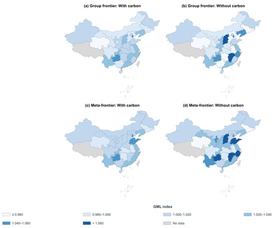
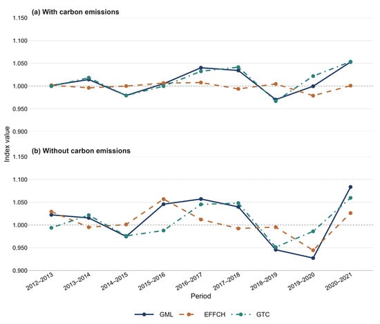
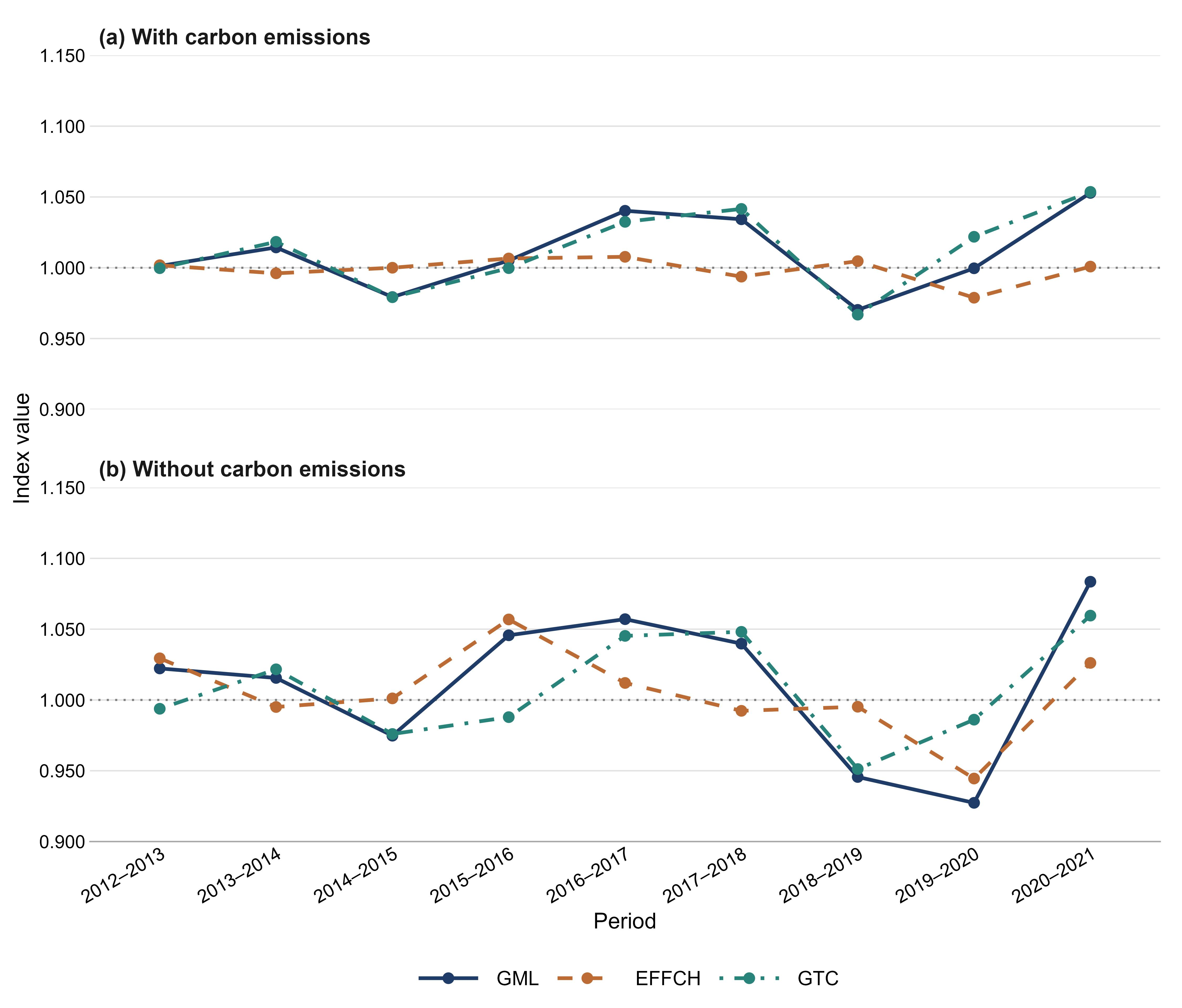
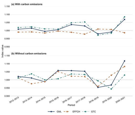
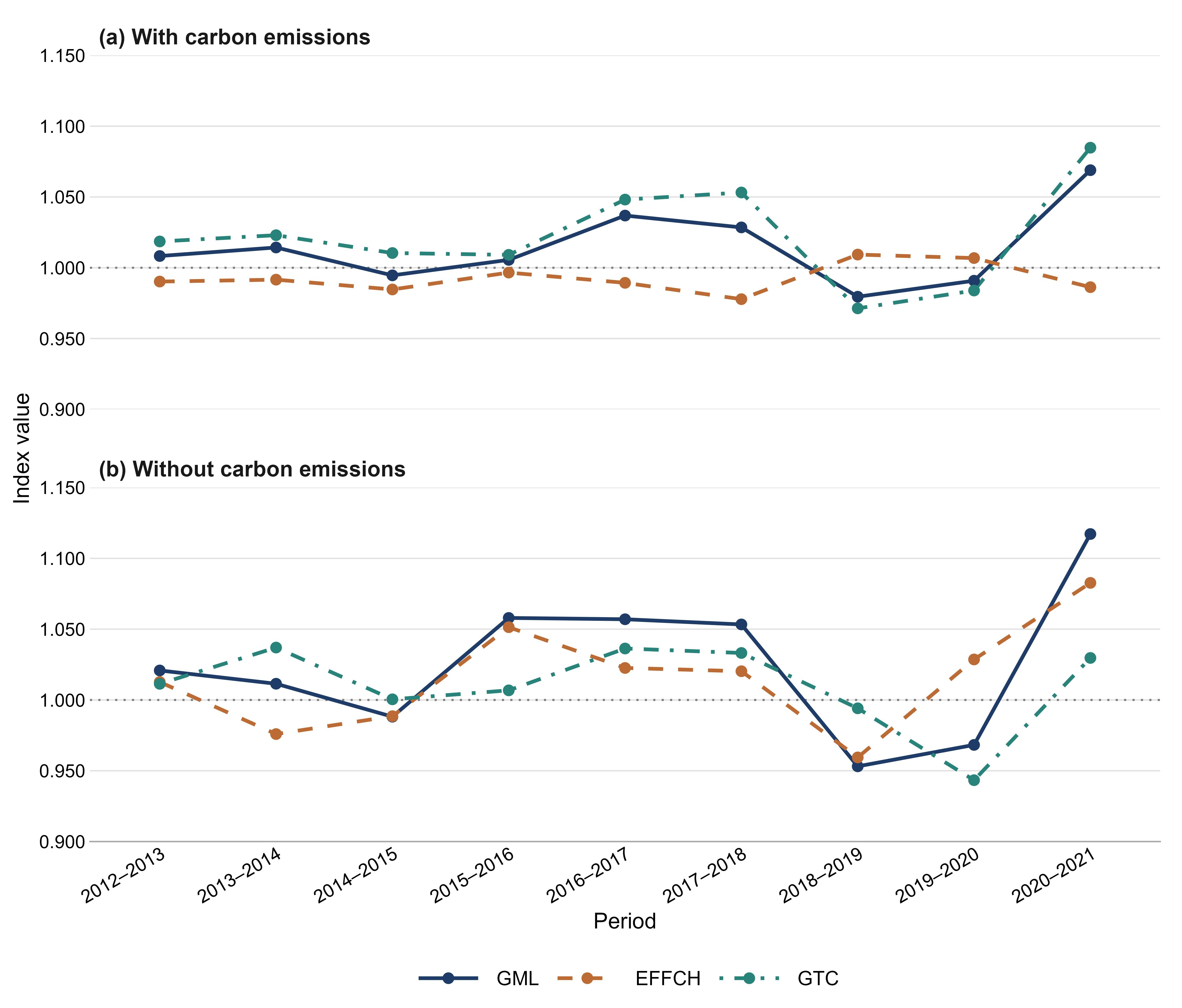

Disclaimer/Publisher’s Note: The statements, opinions and data contained in all publications are solely those of the individual author(s) and contributor(s) and not of MDPI and/or the editor(s). MDPI and/or the editor(s) disclaim responsibility for any injury to people or property resulting from any ideas, methods, instructions or products referred to in the content. |
© 2026 by the authors. Licensee MDPI, Basel, Switzerland. This article is an open access article distributed under the terms and conditions of the Creative Commons Attribution (CC BY) license.