


Abstract
Shot hole disease is one of the major diseases affecting the health of peach trees. To achieve effective grading-based prevention and control and enable precise grading of peach leaf shot hole disease severity, this study proposed a disease grading method based on hyperspectral imaging (HSI) combined with machine learning and deep learning. First, hyperspectral imaging equipment was used to acquire region-of-interest (ROI) information from leaves at different disease grades; after calibration, shot hole disease was divided into five disease grades from Grade 0 to Grade 4. Second, to fully exploit the spectral information, multiple preprocessing methods were systematically compared, and the grading performance of seven machine learning classifiers and two deep learning classifiers under full-spectrum conditions was evaluated. To reduce data dimensionality and redundancy, eight feature wavelength selection methods were introduced, and the performance metrics of the classifiers under different feature wavelengths were compared and analysed. The experimental results showed that scatter correction was the most effective preprocessing strategy at the leaf level: the standard normal variate transformation (SNV) combined with the Elman recurrent neural network reached the highest spectrum-level test accuracy, 77.17%, together with 100% at the leaf level and 94.12% for the leaf-mean spectra, and the linear classifiers logistic regression and linear discriminant analysis reached 94.12% at the leaf level under several preprocessing schemes. Savitzky–Golay smoothing combined with the first derivative (SG+D1) remained clearly superior to the raw spectra, and its combination with the support vector machine (SVM) reached 70.08% at the spectrum level and 76.47% at the leaf level. In terms of feature wavelength selection, eight variable selection methods were compared. The experimental results showed that feature wavelength selection effectively reduced data dimensionality while causing a certain degree of accuracy loss; among the feature-wavelength configurations, the best spectrum-level test accuracy was obtained with the stepwise informative spectral screening (SISS) subset combined with logistic regression (66.93%, and 82.35% at the leaf level), whereas the best leaf-level result of the ten-band subsets was obtained by the synergy interval partial least squares (siPLS) subset with the k-nearest neighbours classifier (94.12%); all the feature subsets remained clearly below the best full-spectrum result, making the accuracy–dimensionality trade-off explicit. Finally, the results indicated that HSI combined with spectral preprocessing can effectively achieve accurate identification of peach leaf shot hole disease grades under full-spectrum conditions, and feature wavelengths can effectively reduce data dimensionality while maintaining a certain level of accuracy. This study provides methodological support and an experimental basis for the precise grading, prevention, and control of peach leaf shot hole disease.
1. Introduction
Peach trees are among the most important economic fruit trees in China, and their fruits, which are rich in nutrients and delicious in taste, hold important dietary and economic value among fruit agricultural products [1]. However, peach tree diseases occur frequently, seriously restricting fruit yield and quality. Among them, peach shot hole disease, caused by bacterial pathogens, is one of the most destructive foliar diseases [2]. This disease spreads rapidly under low-temperature and high-humidity conditions. In the early stage, water-soaked spots form on the leaves; subsequently, the lesions dry and fall off, forming holes. This reduces the photosynthetic area of the leaves and causes premature defoliation, which in turn weakens tree vigor, affects flower bud differentiation and fruit development, and ultimately results in severe economic losses [3]. At present, the assessment of peach leaf shot hole disease severity mainly relies on growers visually observing the leaves in the field and performing empirical grading based on the proportion of lesion area or the number of holes [4]. This traditional investigation method is subjective, inefficient, and inconsistent among different personnel, making it difficult to achieve objective and rapid detection. Accurately detecting and grading the occurrence degree of peach leaf shot hole disease is of important scientific significance and production guidance value for achieving precision pesticide application and reducing pesticide residue [5]. Therefore, developing an objective and accurate grading method for shot hole disease has become an urgent problem to be solved.
In recent years, with the rapid development of computer vision technology, intelligent identification of peach tree diseases based on image analysis has made remarkable progress; however, most studies have focused on the binary discrimination of healthy and diseased leaves or the multi-class classification of different disease types [6]. For the specific type of peach bacterial shot hole disease, Liu et al. [7] proposed the YOLO–PSH detection model to address problems such as large variation in disease characteristics and complex backgrounds under natural conditions, achieving an average detection accuracy of 81.49% and establishing a regional disease severity grading method based on the detection results. Yadav et al. [8] applied deep learning methods to the identification of peach bacterial diseases, and the proposed CNN model achieved an accuracy of 98.75%. Akbar et al. [9] proposed a lightweight WLNet model based on VGG-19, achieving an accuracy of 99% in the classification of peach bacterial diseases. Alhwaiti et al. [10] used the YOLOv4 model to detect bacterial spots on peach leaves, achieving an accuracy of 98%. The above studies demonstrate great application potential in the field of peach tree disease detection; however, fine-grained grading of leaf disease severity remains relatively scarce.
Notably, hyperspectral imaging (HSI) technology has been widely applied in recent years to the quality detection and disease diagnosis of peach fruits and leaves. Bian et al. [11] proposed a multi-scale deformable three-dimensional convolutional neural network (MSD-3DCNN) that can effectively detect the presence or absence of shot hole disease, achieving precision, recall, and F1 scores all above 97% using hyperspectral imaging data. Sun et al. [12] used hyperspectral reflectance imaging combined with a deep belief network to classify three postharvest fungal diseases of peach fruits, achieving an accuracy of 100% for severely rotten samples. Liu et al. [13] combined hyperspectral imaging with chemometrics to achieve quantitative prediction and visualization of the number of fungal contamination colonies in peach fruits. Chen et al. [14] proposed a peach tree disease identification and segmentation framework based on multi-source data fusion, achieving a detection accuracy of 94%. The study of Gong et al. [15] also showed that a spectrum–image dual-modality fusion strategy can markedly improve the accuracy and efficiency of classification systems. The above studies indicate that HSI can simultaneously capture the internal molecular composition changes and external phenotypic characteristics of leaves or fruits and possesses the advantage of integrating spectral and spatial information, making it particularly suitable for detecting and diagnosing stress at early stages when visible symptoms are not obvious [16]. Although some studies have applied HSI to peach disease detection, research on its use for grading peach leaf shot hole disease remains lacking.
In this study, peach leaves with shot hole disease at different severity levels were used as the research objects, and the intrinsic relationship between disease grades and leaf spectral responses was explored based on HSI. Compared with traditional grading methods that rely on visible symptoms, spectral features can capture the internal physiological and biochemical stress information of leaves. To this end, this paper systematically compared the grading performance of full-spectrum spectral data under different preprocessing and classifier configurations and further introduced multiple feature wavelength selection strategies to identify sensitive wavelengths highly correlated with shot hole disease severity and to reveal the key spectral intervals of differences among grades. By comparing the modelling effects of full-spectrum and feature-wavelength data, the balance between reducing model complexity and maintaining grading accuracy through feature selection was evaluated, aiming to provide accurate and operable methodological support for the precise grading, prevention, and control of peach leaf shot hole disease.
2. Materials
2.1. Sample Preparation
Peach leaf samples were collected from a standardized peach orchard in the Xiaotangshan National Precision Agriculture Demonstration Base in Beijing, as shown in Figure 1. Peach leaves with shot hole disease were collected from late July to mid-August 2025, covering leaves with different degrees of disease incidence. After picking, the leaves were placed in sealed bags, and hyperspectral image acquisition was completed within 2 h to maintain the physiological state of the leaves as stable as possible.
Figure 1.
Symptoms of shot hole disease in a peach orchard: (a–c) representative leaves imaged at a higher resolution, in which the red circles mark the typical shot holes (lesions).
The disease studied was peach bacterial shot hole disease. Referring to the industry standard [17], expert opinions, and growers’ experience, the disease severity was graded by the percentage of lesion area in the total area of a single leaf, dividing the disease severity into five grades (Grades 0–4). The detailed grading criteria are presented in Table 1.
Table 1.
Grading standard for peach leaf shot hole disease severity.
The lesion area used as the reference for the grading was determined by two trained assessors together with the growers of the orchard. For each leaf, the lesions and the holes were manually delineated in the ENVI 5.6(64-bit) environment with the region-of-interest drawing tools of the software, the ratio between the delineated lesion area and the total leaf area was calculated automatically, and the final grade was assigned by combining this measured percentage with the expert judgement and the field experience of the growers, following the procedure of the industry standard [17]. The two assessors graded the leaves independently, and any leaf for which the two gradings disagreed was re-examined; the reference label obtained in this way is a leaf-level reference rather than a pixel-level one.
For the spectral measurement, 6–10 regions of interest (ROIs) were delineated on each leaf on the yellowish tissue surrounding the shot holes, and the centre of each perforation was avoided, so that the spectra of the chlorotic halo rather than those of the holes were collected. The mean spectrum of each ROI was extracted and treated as one spectral sample, and 1270 ROI-mean spectra were obtained from the 163 leaves. For the leaves of Grade 0, which showed no lesions, the ROIs were placed on the central and marginal regions of the blade in the same number as for the diseased leaves.
2.2. Hyperspectral Imaging System
This study adopted the hyperspectral imaging system (SOC710Enhanced) developed by Surface Optics Corporation of the United States. The system consists of an imaging spectrometer, a high-sensitivity CCD area-array detector, an internal precision scanning mechanism, and a control unit. The spectral wavelength range is 386.6–1042.6 nm, covering the visible to near-infrared region; the spectral sampling interval is approximately 2.53 nm, and a total of 260 continuous bands are acquired; the spatial resolution is 696 × 696 pixels, enabling high-fidelity imaging of the subtle lesion regions in peach leaf samples. During acquisition, each exposure obtains the entire spectral curve of one column of spatial pixels, and area scanning is achieved through the uniform internal movement of the scanning mechanism, thereby constructing the hyperspectral hypercube data of the target region. Only the 400–950 nm interval, i.e., 218 of the 260 bands (401.1–947.8 nm in the calibrated spectra), was used in the analysis reported below.
To ensure the stability and uniformity of illumination during acquisition, the entire imaging system was integrated into a sealed dark box, and the inner walls of the box were lined with black light-absorbing material to reduce interference from ambient stray light. Two halogen lamps with a rated power of 125 W were used as the light sources, arranged above both sides of the sample stage at a symmetrical incident angle of 45° to illuminate the samples, forming a uniform illumination field in the field of view. The colour temperature of the halogen lamps was 3000 K. Their emission spectrum is a continuous, line-free continuum spanning approximately 350–2500 nm that peaks near 1000 nm in the near-infrared and closely approximates black-body radiation, and their radiant flux is stable, with a drift of less than 1% after a warm-up period of 15–30 min. The spatial scanning of the instrument is performed internally: the sensor translates behind the lens, and this internal translation rate is tied to the exposure parameters of the system, so that no external translation or sample stage movement is required during acquisition. Consequently, the exposure time was 40 ms per scanning line.
2.3. Data Processing Equipment
The hardware platform for network training was mainly configured as follows: an Intel i9-12900K central processing unit, 32 GB DDR5 random access memory, and an NVIDIA GeForce RTX 4070 Ti Super graphics processing unit, with CUDA acceleration used to accelerate the training process. The operating system was Windows 10 Pro for Workstations (version 22H2), the CUDA version was 12.4, and the PyTorch version was 2.4.1 (the corresponding cuDNN version was 9.1.0).
3. Methods
The overall experimental process consisted of six parts: hyperspectral image acquisition and processing, dataset partitioning, data preprocessing, feature selection and extraction, model establishment, and result evaluation. The overall experimental flowchart is shown in Figure 2.
Figure 2.
Overall experimental flowchart.
3.1. Hyperspectral Image Acquisition and Processing
The samples were placed horizontally on a black sample stage. Control and acquisition were implemented with the supporting software HyperScanner 2.0, through which single-band grayscale images could be previewed in real time and key imaging parameters could be adjusted. Based on the pre-experiment optimization, the exposure time of a single scan was fixed at 40 ms, the optical axis of the imaging lens was perpendicular to the plane of the sample stage, and the distance between the front end of the lens and the sample plane was strictly set to 50 cm. Finally, calibration was performed using the standard panel ratio method, and the calibration process was executed with the supporting batch processing software SRAnal710e.bat. Under the above parameter combination, the spectral images exhibited an excellent signal-to-noise ratio and could truly reflect the reflection characteristics of the leaves at different wavelengths. The spectral reflectance of peach leaf shot hole disease is shown in Figure 3, and the average reflectance of the different disease grades is shown in Figure 4.
Figure 3.
Reflectance spectral curves of all samples.
Figure 4.
Average spectral reflectance curves of the five disease grades.
3.2. Dataset Partitioning
In this study, the dataset consisted of 163 leaves and 1270 ROI-mean spectra; for Grades 0–4 the numbers of leaves were 30, 35, 38, 30 and 30, and the numbers of spectra were 210, 300, 330, 210 and 220, respectively (Table 2). For the results reported in Section 4, the partition was performed jointly on the leaves and on the spectra: the total number of spectra was counted first, and whole leaves were then assigned to the training, the validation and the test subset so that the number of spectra of every grade followed the 8:1:1 ratio and the grade proportions were preserved (Table 2). Each leaf was therefore assigned to exactly one subset, and the spectra of one leaf were never divided between the three subsets: the training, the validation and the test subset contained 129, 17 and 17 leaves and 1016, 127 and 127 spectra, respectively, and the numbers of leaves per grade were 24, 27, 30, 24 and 24 in the training subset, 3, 4, 4, 3 and 3 in the validation subset and 3, 4, 4, 3 and 3 in the test subset (Table 2). As a consequence of this leaf-level partition, the ROIs of one leaf cannot appear in the training subset and in the test subset at the same time, so that the ROIs of a leaf are never divided between the subsets. All preprocessing parameters, scalers, wavelength-selection procedures and classifier hyperparameters were derived from the training data only; the validation subset was used for threshold tuning and for early stopping, and the test subset was used only for the final evaluation. Because the ROI spectra of one leaf are strongly correlated with each other, the leaf, and not the ROI spectrum, is the statistical unit of the evaluation: the accuracy of every configuration is reported at the spectrum level and at the leaf level, and the uncertainty of the main configuration is estimated by resampling whole leaves (Section 3.6).
Table 2.
Data distribution.
3.3. Spectral Preprocessing Methods
In addition to the chemical information related to peach leaf shot hole disease, the raw hyperspectral data were also disturbed by various non-target factors, such as sample background scattering, optical path variations, and random noise; direct modelling could easily lead to a decline in model stability and generalization ability.
To eliminate or suppress the above interference, this study adopted the following strategies to construct a set of preprocessing methods. First, Savitzky–Golay convolution smoothing [18] (SG) was uniformly applied to the full-spectrum raw spectra. SG smoothing fits local data windows through polynomial least squares, suppressing instrument and environmental noise while preserving the peak shape information of the spectra; the polynomial order and window half-width need to be optimized according to the spectral resolution and signal-to-noise ratio to filter out high-frequency random noise while retaining the effective chemical absorption features in the spectral profile. Taking the SG-smoothed spectra as the baseline, the standard normal variate transformation [19] (SNV) was further combined, which is also used to correct the scattering caused by optical path variations. By mean-centring each spectrum and dividing it by its standard deviation, the spectral data approximately follow a standard normal distribution, making it particularly suitable for the cases where the scattering effects in the spectra are wavelength-dependent. The first-derivative (D1) and second-derivative (D2) algorithms can eliminate baseline drift and enhance the resolution of overlapping peaks while further suppressing low-frequency background interference; however, derivative calculation amplifies high-frequency noise, and therefore it is combined with SG smoothing beforehand. Eight preprocessing combinations were formed: Raw (raw spectra), SG, SG+D1, SG+D2, SNV, SG+SNV, SG+SNV+D1, and SG+SNV+D2. The Savitzky–Golay smoothing was applied with a window length of 11 points and a second-order polynomial, and the first and second derivatives were computed with the same Savitzky–Golay filter; before modelling, all features were standardized to zero mean and unit variance with a scaler that was fitted on the training data only and then applied unchanged to the validation and the test data.
The above preprocessing combinations covered typical pairings of the three processing logics of smoothing, correction, and derivative enhancement, enabling a systematic evaluation of the effects of different preprocessing strategies for the peach leaf shot hole disease grading task of this study.
3.4. Feature Wavelength Selection Methods
Hyperspectral data contain numerous bands, and severe collinearity exists among adjacent bands. Full-spectrum modelling not only incurs high computational costs but also makes the model prone to overfitting and reduces interpretability due to redundant information. Feature wavelength selection aims to select the most compact subset rich in discriminative information from hundreds of bands, thereby improving model robustness and computational efficiency. In this study, eight representative variable selection algorithms were adopted to screen key wavelengths from the full spectra or the preprocessed spectra based on different principles.
Competitive adaptive reweighted sampling [20] (CARS) constructs partial least squares models through multiple Monte Carlo samplings and retains the strongly correlated bands according to the absolute values of the regression coefficients while adaptively reducing the number of retained wavelengths; the subset with the minimum root mean square error of cross-validation is finally adopted as the feature wavelengths. The successive projections algorithm [21] (SPA) is a forward variable selection method that selects the band combination with the lowest collinearity through iterative projection operations, aiming to minimize redundancy and maximize the coverage of the vector space; the resulting subset has natural resistance to collinearity problems. Synergy interval PLS [22] (siPLS) divides the full-spectrum into several equal intervals and constructs PLS models with arbitrary combinations of intervals, determining the optimal interval combination through cross-validation errors and thereby preserving the synergy effects of broad spectral regions. The shuffled frog leaping algorithm [23] (SFLA) is based on the memetic algorithm framework, encoding variable subsets as frog individuals and achieving population evolution through local deep search and global information exchange, balancing convergence speed and solution diversity. Iteratively retained informative variables [24] (IRIV) is based on binary matrix shuffling and mean square error evaluation, selecting bands through variable classification and iterative elimination strategies. Variable importance in projection [25] (VIP) originates from the PLS model and quantifies the explanatory contribution of each band to the response variable in the form of a weighted sum of squares, and VIP > 1 is usually adopted as the threshold for selecting important bands. The variable iterative space shrinkage approach [26] (VISSA) combines model population analysis with a soft shrinkage strategy, gradually shrinking the variable space through multiple rounds of modelling and finally obtaining the band subset with the best prediction performance. Stepwise informative spectral screening [27] (SISS) estimates the informative contribution of each wavelength with a random-forest regression model and then screens the wavelengths by this importance ranking, so that weakly informative wavelengths are removed; the highest-ranked wavelengths are retained as the feature subset, which reduces redundancy while preserving the most informative spectral channels.
Each algorithm has its applicable conditions. In this study, multiple selection strategies were systematically compared to reveal the distribution patterns of the spectrally sensitive bands of peach leaf shot hole disease and to provide high-quality inputs for the subsequent classification models.
The parameter settings of the eight selection routines were as follows. For CARS, 50 Monte Carlo runs were performed, each run containing 30 sampling iterations with a sampling ratio of 0.8, the maximum number of latent variables was 5, and the number of retained wavelengths was fixed at 10. For SPA, the wavelengths were selected by forward iterative projection with the same fixed subset size of 10. For siPLS, the 400–950 nm range was divided into 10 equal-width intervals, 5 intervals were jointly selected by cross-validation, and the 2 highest-ranked wavelengths of each selected interval were retained, giving 10 wavelengths in total. For SFLA, the population contained 10 frogs, 30 local search iterations were performed, and the fitness of a candidate subset was defined as the cross-validated classification error of a PLS-DA model built on this subset. For IRIV, 15 iterations were performed with 80 binary matrix shuffling repetitions per iteration, the maximum number of latent variables was 5, and a five-fold cross-validation was used. For VIP, the scores were computed from a PLS model with 5 latent variables, and the 10 wavelengths with the largest scores were retained. For VISSA, the variable space was shrunk by the factor α = 0.8 per iteration, at most 200 iterations were allowed, and the shrinkage was stopped when 10 wavelengths remained.
3.5. Classification Methods
To comprehensively evaluate the benefits of preprocessing and wavelength selection for peach leaf shot hole disease grading, this study adopted seven classical machine learning classifiers and two deep learning classifiers, constructing a multi-level classification model pool ranging from linear discrimination to nonlinear ensembles and from traditional machine learning to one-dimensional convolutional neural networks.
The support vector machine [28] (SVM) uses a radial basis function (RBF) kernel to map the low-dimensional spectral data into a high-dimensional feature space to seek the maximum-margin hyperplane; the kernel width γ and the regularization parameter C were determined by grid search and cross-validation (the final values for the full-spectrum SG+D1 configuration were γ = ‘auto’ and C = 10; the search space covered C ∈ {0.1, 1, 10, 100} and γ ∈ {scale, auto, 0.01, 0.001}). The random forest [29] (RF) builds a large number of decision trees through bootstrap resampling and random feature subspaces and outputs the class labels by majority voting, exhibiting strong resistance to overfitting and insensitivity to hyperparameters (n_estimators = 200, class_weight = ‘balanced’). Partial least squares discriminant analysis [30] (PLS-DA) takes latent variables as the inputs, encodes the grades as a response matrix for regression, and then sets thresholds for classification, combining dimensionality reduction and modelling; the number of latent components was set to min(15, N), where N is the number of input variables. The k-nearest neighbours [31] (KNN) algorithm directly makes decisions by voting based on the distance measures in the feature space; Euclidean distance was used as the distance metric and the number of neighbours was set to k = 5. Logistic regression [32] (LR) is based on multi-class softmax regression and adopts L2 regularization to prevent overfitting (C = 1, max_iter = 1000). Linear discriminant analysis [33] (LDA) assumes that each class follows a Gaussian distribution with unequal means but identical covariance matrices and seeks the projection direction that maximizes the ratio of between-class scatter to within-class scatter, making it suitable for linearly separable spectral distributions (solver = ‘svd’). Gaussian naive Bayes [34] (GNB) is based on Bayes’ theorem and the conditional independence assumption of features, modelling with Gaussian probability densities; although the assumption is strong, it is often robust for high-dimensional spectral data with small sample sizes (default parameter settings were used).
In addition to the above traditional models, two deep learning models were adopted: the one-dimensional convolutional neural network (1D-CNN) [35] and the Elman recurrent neural network (ELMAN) [36]. The network structure from the input to the output is as follows: the input layer receives a feature band vector with a length of N; the first convolutional layer uses 16 one-dimensional convolution kernels with a size of 3, a stride of 1, and padding to maintain the length, followed by the ReLU activation function; the first max-pooling layer uses a pooling kernel size of 2 and a stride of 2 to reduce the dimensionality; the second convolutional layer is configured with 32 convolution kernels with a size of 3, also followed by ReLU; the second pooling layer has the same parameters as the first; subsequently, the feature maps are flattened into a one-dimensional vector and fed into a fully connected layer containing 128 neurons with the ReLU activation function, and a dropout probability of 0.3 is applied after this layer to suppress overfitting; the output layer is a Softmax classifier whose number of nodes equals the number of shot hole disease grades K. For the ELMAN network, the input vector of length N is treated as a single-time-step sequence; the recurrent layer is an Elman-type RNN with 64 hidden neurons, the ReLU activation function is applied to the last hidden state, and the output is produced by a fully connected layer with K nodes. The 1D-CNN and ELMAN models were implemented and trained based on the PyTorch 2.4.1 framework for all deep-learning runs, so that repeated training runs with the same configuration yield identical results on the same platform. The optimizer was AdamW, the initial learning rate was set to 1 × 10⁻³, the momentum parameters were β1 = 0.9 and β2 = 0.999, and the weight decay coefficient was 1 × 10⁻⁴. The batch size was set to 128, and the total number of training epochs was 300; mini-batches were formed by randomly shuffling the training samples, and no stratification was applied during batch creation (the overall training/validation/test split was stratified by grade). The model weights corresponding to the highest validation accuracy over the 300 epochs were restored for evaluation; no learning-rate scheduling or early stopping was used.
3.6. Evaluation Metrics
Four metrics were selected as the quantitative evaluation metrics of model performance [37]: the spectrum-level accuracy (Spec. Acc, %), the leaf-level accuracy (Leaf Acc, %), the leaf-mean accuracy (Leaf-mean Acc, %) and the macro F1-score (MacF1). The three accuracy levels are distinguished in the results, in accordance with the leaf-disjoint partition of Section 3.2: the spectrum-level accuracy is obtained by classifying each ROI-mean spectrum independently, the leaf-level accuracy by majority voting over the ROI spectra of a leaf, and the leaf-mean accuracy by first averaging the ROI spectra of a leaf and then classifying the resulting mean spectrum. The macro F1-score is computed from the leaf-level predictions of the corresponding configuration, and the per-grade accuracies shown in the radar charts are obtained from the leaf-mean spectrum of each test leaf. The uncertainty of the main configuration is estimated by a cluster bootstrap that resamples whole leaves instead of individual spectra, and the robustness of the comparison is assessed by a repeated grouped five-fold cross-validation over all 163 leaves of the dataset.
4. Results
4.1. Spectral Preprocessing Results
As the front-end stage of hyperspectral data modelling, spectral preprocessing aims to eliminate non-informative variations, such as instrument noise, scattering effects, and baseline drift, while enhancing the spectral features related to the target attribute. In this study, eight preprocessing schemes were investigated: raw spectra (Raw), Savitzky–Golay smoothing (SG), first derivative (SG+D1), second derivative (SG+D2), standard normal variate transformation (SNV), and their composite strategies (SG+SNV, SG+SNV+D1, and SG+SNV+D2). The processing results are shown in Figure 5.
Figure 5.
Spectral preprocessing results.
4.2. Grading Results of the Eight Preprocessing Methods Combined with the Nine Classifiers Under Full-Spectrum Conditions
Under full-spectrum conditions, eight spectral preprocessing strategies, namely Raw, SG, SG+D1, SG+D2, SNV, SG+SNV, SG+SNV+D1, and SG+SNV+D2, were systematically combined with nine classifiers, namely SVM, RF, PLS-DA, KNN, LR, LDA, GNB, ELMAN, and 1D-CNN, for combined modelling, and the overall effectiveness of the models was evaluated using the four evaluation metrics defined in Section 3.6.
The overall performance metrics are shown in Figure 6. The experimental results indicated that the choice of the preprocessing method had a substantial impact on the grading performance and that this impact exhibited an obvious interaction effect across different classifiers, while the absolute values were markedly lower than those obtained when the individual ROI spectra were treated as independent observations. Under the leaf-disjoint partition the highest spectrum-level test accuracy, 77.17%, was obtained with the standard normal variate transformation (SNV) combined with the ELMAN network, which also gave the highest leaf-level accuracy of all the full-spectrum configurations (100%, i.e., the 17 test leaves were all graded correctly by majority voting) together with a leaf-mean accuracy of 94.12%; the same spectrum-level accuracy was obtained by SNV combined with logistic regression, with 94.12% at both the leaf level and the leaf-mean level. The linear classifiers were in general the most accurate at the leaf level: logistic regression and linear discriminant analysis reached 94.12% under several preprocessing schemes, including SG+D1, SG+D2, SNV and SG+SNV+D1, whereas their spectrum-level accuracies ranged from 66.14% to 77.17%. The derivative preprocessing remained clearly better than the raw spectra for the SVM (SG+D1: 70.08% at the spectrum level and 76.47% at the leaf level, against 61.42% and 64.71% without preprocessing) and for the 1D-CNN (65.35% and 76.47%), and SG+SNV+D1 combined with the SVM gave 73.23% at the spectrum level together with 88.24% at the leaf level. Among the composite strategies, SG+SNV+D1 was the most effective, whereas SG+SNV alone did not exceed SNV. Notably, the GNB classifier performed worse than the other classifiers under all the preprocessing conditions, with a spectrum-level accuracy of 40.16–62.20% and a leaf-level accuracy of 41.18–64.71%; this classifier was the one most strongly affected by the preprocessing scheme, its spectrum-level accuracy increasing from 40.16% without preprocessing to 59.84% under SNV and SG+SNV, a relative increase of about 49%. This indicates that the naive Bayes classifier is highly sensitive to the distribution characteristics of spectral data and that adequate preprocessing plays a key role in improving its performance. Because the test subset contains only 17 leaves, the differences between the leading configurations are comparable to the width of the leaf-level confidence interval discussed in Section 5.3, and the ranking of individual model pairs is therefore reported descriptively rather than as a formal ordering.
Figure 6.
Performance of the eight preprocessing methods with the full-spectrum on the leaf-disjoint partition. Columns: Spec. Acc, Leaf Acc, Leaf-mean Acc and MacF1.
The per-grade accuracy results are shown in Figure 7, in which the per-grade values are those obtained by classifying the leaf-mean spectrum of each test leaf. Taking the SNV–ELMAN combination, which achieved the highest spectrum-level accuracy, as an example, Grades 0–3 were graded perfectly (1.000) and the accuracy of Grade 4 was 0.667; the SG+D1–SVM combination classified Grades 0 and 2–4 perfectly, whereas its accuracy for Grade 1 fell to 0.500, which indicates that the first-derivative preprocessing still confuses part of the Grade 1 leaves with the adjacent grades. The 1D-CNN classifier under SG+D1 preprocessing gave 1.000, 0.500, 0.500, 1.000 and 1.000 for Grades 0–4, again with the lowest values for Grades 1 and 2, and a different pattern was observed for the SNV–RF combination, whose accuracies were 0.333, 0.500, 0.750, 1.000 and 0.667, so that here Grade 0 was the weakest. Comparing the per-grade behaviour of each classifier under the Raw condition, the accuracies of the SVM without preprocessing were 0.667, 0.250, 1.000, 0.667 and 0.000; after SG+D1 preprocessing, the accuracy of the SVM for Grade 1 rose from 0.250 to 0.500 and that of Grade 4 from 0.000 to 1.000, indicating that first-derivative preprocessing extracts the differentiated spectral information of the diseased grades more effectively. The linear classifiers were less balanced in the opposite direction: LDA and LR classified Grades 0–3 correctly under most preprocessing schemes but reached only 0.667 for Grade 4, the grade with the largest lesion area. Taken over all 72 full-spectrum configurations, Grade 3 was the best-recognised grade (mean leaf-mean accuracy 0.921) and Grade 4 the least well recognised (0.699).
Figure 7.
Radar chart of the per-grade accuracies of the eight preprocessing methods on the leaf-disjoint partition.
Combining the two dimensions of overall performance and per-grade accuracy, the full-spectrum analysis indicated that the scatter-correction preprocessing (SNV) and the composite strategy SG+SNV+D1 were the most effective preprocessing schemes under the leaf-disjoint evaluation, and that the linear classifiers (LR and LDA) and the deep networks were the most accurate models. The three-panel confusion matrix of the best full-spectrum configuration, SNV–ELMAN, is shown in Figure 8; at the spectrum level the errors were almost entirely assignments to an adjacent grade, the majority vote over the ROI spectra of each test leaf classified all 17 leaves correctly, and at the leaf-mean level, only one Grade 4 leaf was assigned to Grade 2. In addition, the deep learning classifiers 1D-CNN and ELMAN also demonstrated good grading potential under full-spectrum conditions and exhibited relatively low dependence on preprocessing. Although the GNB classifier benefited from adequate preprocessing, its absolute performance still remained below that of the other classifiers, and its use in practical applications should be considered cautiously.
Figure 8.
Confusion matrices of the best full-spectrum configuration (SNV–ELMAN).
4.3. Analysis of Wavelength Selection Results of Different Feature Extraction Algorithms
With the Savitzky–Golay combined with first-derivative preprocessing fixed, this study further compared the effects of eight feature wavelength extraction methods, namely CARS, SPA, siPLS, SFLA, IRIV, SISS, VIP and VISSA, on the grading performance. Based on the bands selected by the eight algorithms within the analysed spectral range of 400–950 nm, the distribution of the selected wavelengths and the preferences of the algorithms for spectral regions were analysed, and the results are shown in Figure 9. The eight algorithms differed in the regions on which they concentrated. CARS selected two isolated bands at 678.1 and 700.8 nm, a compact two-band block at 731.2–733.8 nm, a further group of three bands at 864.6, 867.2 and 877.5 nm, a closely spaced pair at 890.5 and 898.3 nm and one further band at 908.7 nm, so that its sparse pattern extends to 908.7 nm; VIP selected one continuous narrow cluster at 723.6–746.5 nm; SPA formed one continuous block at 523.4–545.6 nm in the green region; SISS selected the 635.3–642.8 nm block, the 731.2–744.0 nm block and the 864.6–867.2 nm pair; SFLA and IRIV selected isolated bands over the widest intervals of the eight subsets (413.3–906.1 nm and 567.9–934.8 nm, respectively), followed by siPLS (560.5–885.3 nm); and VISSA selected 432.7 and 660.4 nm, a pair at 700.8–703.3 nm and the 731.2–736.3 nm block together with sparse bands up to 890.5 nm. The red-edge cluster around 731–736 nm was included by five of the eight methods, which confirms the importance of this region for the disease grades but also means that part of the subset content is common to several methods. The overlap between CARS and VIP was limited to two bands, and six bands were shared by CARS and VISSA—three of them in the 701–734 nm region, together with 864.6, 877.5 and 890.5 nm; both routines weight the PLS regression coefficients, so their partial convergence on the same informative region is expected, but the remaining bands of the two subsets differed and their grading results also differed.
Figure 9.
Feature wavelengths extracted by different algorithms within the analysed 400–950 nm window. Solid curves: mean reflectance of Grades 0–4; red dashed lines: selected bands.
In contrast, the bands selected by SISS, VISSA, SFLA and siPLS were more dispersed over the spectrum. SISS selected a four-band block at 635.3–642.8 nm, a four-band block at 731.2–744.0 nm and the 864.6–867.2 nm pair, so that a visible-region block and a red-edge block were combined with isolated near-infrared bands; this subset reached its best spectrum-level test accuracy of 66.93% with logistic regression (82.35% at the leaf level) and with the 1D-CNN (88.24% at the leaf level). The bands selected by VISSA were distributed between 432.7 and 890.5 nm as an isolated band at 432.7 nm, a pair at 660.4 and 700.8–703.3 nm and the 731.2–736.3 nm block, followed by three near-infrared bands. The bands selected by SFLA covered the interval from 413.3 to 906.1 nm, with five bands at or above 721.1 nm. The bands selected by siPLS were spread over 560.5–885.3 nm, with 685.6 and 693.2 nm near the red edge and sparse bands in the near-infrared region (820.7–885.3 nm); the grading behaviour of the siPLS subsets was nevertheless strongly classifier-dependent, their leaf-level accuracy ranging from 47.06% to 94.12%.The complete lists of the selected wavelengths are given in Table A1 of Appendix A, and the corresponding accuracy–dimensionality trade-off is quantified in Table A2.
4.4. Grading Results Under Different Feature Wavelengths After SG+D1 Preprocessing
The overall performance metrics are shown in Figure 10. The choice of the feature extraction method had a clear influence on the final grading accuracy, and the feature subsets differed in their information content. In terms of the spectrum-level test results, the highest accuracy among all the feature-subset configurations was obtained by the SISS subset, both with logistic regression (66.93% at the spectrum level and 82.35% at the leaf level) and with the 1D-CNN (the same 66.93% at the spectrum level and 88.24% at the leaf level), followed by SISS–ELMAN (66.14%) and SISS–SVM (65.35%); the CARS subset combined with the ELMAN network and with the 1D-CNN reached 64.57% and 60.63%, respectively, and CARS–LR and VISSA–ELMAN reached the highest leaf-mean accuracies of the feature grid (88.24% in both cases). When the leaf-level accuracy obtained by majority voting is used instead of the spectrum-level accuracy, the best feature subset was siPLS–KNN at 94.12%, followed by CARS–ELMAN, SISS–1D-CNN and SFLA–KNN, all at 88.24%. The SPA and IRIV subsets were the weakest of the eight methods, their best spectrum-level accuracies being 50.39% (SPA–1D-CNN) and 55.12% (IRIV–SVM), and the IRIV subset was also the least stable: its leaf-mean accuracy with the KNN classifier fell to 23.53%, the lowest value in the whole feature grid. The VIP subset occupied an intermediate position, with a best spectrum-level accuracy of 55.91% (VIP–LDA); the behaviour of the siPLS subset depended strongly on the classifier, its spectrum-level accuracy ranging from 49.61% (siPLS–GNB) to 62.20% (siPLS–KNN) and its leaf-level accuracy from 47.06% to 94.12%. The accuracy loss accompanying the reduction from 218 to 10 bands was substantial for all the methods: the best feature subset remained 10.2 percentage points below the best full-spectrum configuration at the spectrum level (66.93% against 77.17%) and 5.9 points below it at the leaf level (94.12% against 100.00%), and the feature subsets should therefore be regarded as a dimensionality-reduction option with a measurable accuracy cost rather than as an equivalent substitute for the full-spectrum.
Figure 10.
Performance of the eight feature selection methods under SG+D1 preprocessing on the leaf-disjoint partition. Columns: Spec. Acc, Leaf Acc, Leaf-mean Acc and MacF1.
The per-grade accuracy results are shown in Figure 11, in which the per-grade values are those obtained by classifying the leaf-mean spectrum of each test leaf. Different feature extraction methods exhibited different recognition preferences for the disease grades. For the SISS subset, which gave the best spectrum-level test accuracy, the per-grade accuracies with logistic regression were 0.333, 1.000, 1.000, 0.667 and 0.667 for Grades 0–4, with the lowest value for Grade 0; the CARS–ELMAN combination gave 0.667, 0.500, 1.000, 1.000 and 1.000, and the SFLA–KNN combination 1.000, 0.500, 0.500, 1.000 and 1.000, so that the errors of the strongest subsets were again concentrated in the intermediate grades. Very low values occurred for individual grades with the linear and probabilistic classifiers: the accuracy of Grade 0 was 0.000 for VIP–PLS-DA, VIP–LR, VIP–LDA and IRIV–KNN, and that of Grade 3 was 0.000 for several CARS, SPA, siPLS and VIP combinations; the IRIV–KNN combination was the least accurate overall, its leaf-mean accuracy over the five grades falling to 0.235, the lowest value of the feature grid. These results indicate that some feature subsets are not compatible with the assumptions of the linear models and that the per-grade accuracies of a subset depend strongly on the classifier with which it is combined.
Figure 11.
Radar chart of the per-grade accuracies of the eight feature selection methods under SG+D1 preprocessing.
The horizontal comparison of the feature extraction methods showed that the feature subsets retained different amounts of grading information. Under the leaf-disjoint partition, the SISS subset was the most accurate at the spectrum level (66.93%, with logistic regression and with the 1D-CNN), whereas the best leaf-level result was obtained with the siPLS subset and the k-nearest neighbours classifier (94.12%), and the best leaf-mean result was shared by CARS–LR and VISSA–ELMAN (88.24% in both cases). The IRIV and SPA subsets performed unsatisfactorily on this dataset: the feature wavelengths they selected did not capture the discriminative information of all the grades, and some of their per-grade accuracies were 0.000; their selection criteria need further optimization or the introduction of more advanced feature evaluation metrics in future research. Because no single feature subset was the most accurate at all three accuracy levels, the choice of a subset for a specific application depends on which level of the assessment is of interest.
5. Discussion
5.1. Mechanisms Underlying the Effects of Spectral Preprocessing on Model Performance
The core function of spectral preprocessing in hyperspectral modelling is to suppress non-informative variations and amplify target-related spectral features. In this study, the scatter correction (SNV) was the most effective single preprocessing scheme under the leaf-disjoint evaluation, and its combination with the ELMAN network achieved the highest spectrum-level test accuracy (77.17%), together with a leaf-level accuracy of 100%; the derivative-based SG+D1 remained clearly superior to the raw spectra for the classical classifiers, its spectrum-level accuracy exceeding that of the raw spectra by 8.7 percentage points for the SVM (70.08% against 61.42%) and by 11.8 points at the leaf level (76.47% against 64.71%). In the 400–950 nm range, the spectral slopes of the different disease grades in the red-edge region differed noticeably, and the first derivative precisely captured this differential feature, thereby projecting the grades that were difficult to distinguish in the original reflectance space into a more separable feature space.
Standard normal variate transformation (SNV), as a scattering correction method based on sample independence, effectively eliminates the multiplicative scattering effects caused by particle size, surface roughness, and optical path variations through per-spectrum mean centring and standard deviation normalization. The experimental results showed that SNV achieved excellent performance on both the SVM and the LDA, indicating that scattering correction is particularly important for classifiers based on distance metrics and covariance structures: the decision boundary of the SVM depends on the distance distribution of the samples in the feature space, whereas the LDA relies on the covariance matrix estimation of each class; the standardization of the spectral distribution by SNV improves both intra-class cohesion and inter-class separation. However, although SNV improves the symmetry and homoscedasticity of the univariate distributions, it cannot change the inherent strong multicollinearity structure among the spectral bands. The high correlations among the bands seriously violate the conditional independence assumption, leading to distorted posterior probability estimates. The composite preprocessing strategies (such as SG+SNV and SG+SNV+D1) did not exceed the optimal single preprocessing scheme in this study; for the SVM, the accuracy of SG+D1–SVM was markedly higher than that of SG+SNV–SVM in this dataset (Figure 6). A possible explanation is that although the combination of smoothing and normalization can simultaneously suppress multiple noise sources, multi-step processing also faces the risks of parameter interaction and over-correction: the first derivative highlights the rate of spectral change, whereas the standardization operation of SNV may inappropriately scale the derivative amplitudes, thereby distorting the originally effective discriminative gradient information.
5.2. Comparative Analysis of Feature Wavelength Selection for Model Simplification and Accuracy
The core of feature wavelength selection lies in dimensionality reduction, aiming to remove redundant information to reduce the risk of overfitting and improve computational efficiency; however, excessive compression may lose key discriminative information, resulting in accuracy loss. In this study, under the fixed SG+D1 preprocessing condition, the selection results of eight feature extraction algorithms were compared and analysed, and the spectral distribution of the selected wavelengths was found to influence the grading performance, although not in a simple monotonic way. The SISS, CARS, siPLS and SFLA subsets were among the most competitive under the leaf-disjoint evaluation: SISS produced the best spectrum-level test result, both with logistic regression and with the 1D-CNN (66.93% in both cases), siPLS produced the best leaf-level result with the k-nearest neighbours classifier (94.12%), and CARS–ELMAN and SFLA–KNN both reached 88.24% at the leaf level. The IRIV, SPA and VIP subsets were the weakest; the SFLA and IRIV subsets, which were dispersed over the widest intervals (413.3–906.1 nm and 567.9–934.8 nm, respectively), were not among the best-performing configurations at the spectrum level, so the coverage of a wide spectral range alone did not guarantee good grading performance. From the perspective of the spectral mechanisms, the red-edge region was retained by five of the eight methods, and the amplitude of the first derivative in this region is known to vary with the chlorophyll content and the stress status of the vegetation, which makes it a plausible fingerprint region for distinguishing the disease grades; the blue and green bands are sensitive to secondary pigments such as anthocyanins and carotenoids, and the near-infrared region mainly reflects the internal structure and water content of the leaves. These interpretations are hypotheses derived from the literature rather than conclusions of the present experiment, because no biochemical reference measurements were performed. Because the differences among the grades are distributed over different spectral regions, features from a single region alone cannot be expected to support the fine-grained discrimination of all grades. It should also be noted that the deep models did not compensate for the information lost by the weakest subsets: the ELMAN and 1D-CNN classifiers reached their lowest spectrum-level accuracies, 44.88% and 42.52%, respectively, with the VIP subset.
In summary, whether a feature selection algorithm can achieve a good balance between model simplification and accuracy preservation depends on whether it can reduce the statistical dependence among the features while retaining the spectral difference information of the multiple grades, and the comparison showed that this balance was partial: the best feature configuration reached a spectrum-level accuracy of 66.93% and a leaf-level accuracy of 94.12%, i.e., 10.2 and 5.9 percentage points lower, respectively, than the corresponding best full-spectrum values (77.17% and 100.00%), while the number of acquired wavelengths was reduced by 95.4%. This shows that the accuracy cost of the dimensionality reduction is measurable, and the transfer of the subsets to a low-band-count device still requires dedicated hardware validation (Section 5.5); the reduction is, therefore, best regarded as a balanced outcome whose acceptability depends on the requirements of the intended application.
5.3. Comparison of Deep Learning Networks and Traditional Machine Learning Models
This study covered two deep learning models, the one-dimensional convolutional neural network (1D-CNN) and the Elman recurrent neural network (ELMAN), as well as seven traditional machine learning models, providing systematic empirical evidence for the performance comparison between deep learning and shallow models in hyperspectral grading tasks. Under the leaf-disjoint evaluation, the two deep models were among the most accurate configurations of the full-spectrum grid: SNV–ELMAN gave the highest spectrum-level test accuracy (77.17%, with 100% at the leaf level), while the linear classifiers LR and LDA reached 94.12% at the leaf level and 94.12% on the leaf-mean spectra under several preprocessing schemes, so that the deep models were competitive with, but not clearly superior to, the tuned linear models. The numerical pairwise comparisons of the main configurations are treated as descriptive only and are not used to support the conclusions of this study. The test subset contains 127 ROI-mean spectra, but these spectra belong to only 17 leaves and the spectra of one leaf are near-duplicates of each other: the mean correlation between the ROI-mean spectra of the same leaf over the 218 bands of the 400–950 nm window is 0.998, so the number of effectively independent observations is 17 rather than 127. The uncertainty of the headline configuration is therefore reported by a cluster bootstrap that resamples whole leaves, which yields an interval that is markedly wider than the interval obtained when the 127 spectra are treated as independent, and all the comparisons were repeated with a grouped five-fold cross-validation over the 163 leaves of the complete dataset. Formal paired significance testing with a correction for multiplicity remains future work on a larger leaf-level test set.
Compared with the approaches previously reported for peach shot hole disease, the method proposed here has specific advantages and limitations. Deep learning detection methods such as YOLO–PSH [7], the CNN model of Yadav et al. [8], WLNet [9] and YOLOv4 [10] operate directly on leaf images and provide the location of the lesions, whereas the present hyperspectral approach grades severity from the spectral response and is therefore less dependent on the visual quality of the images but requires dedicated acquisition equipment (a line-scan hyperspectral camera (SOC710Enhanced) with 125 W halogen illumination and an internal scanning mechanism inside a dark box, as described in Section 2.2; such a system is considerably more expensive and less portable than a conventional RGB camera [16]). In terms of accuracy, the best value obtained here (77.17%) is lower than the 98.75% and 99% reported by Yadav et al. [8] and Akbar et al. [9], respectively; those values, however, refer to the classification of disease types rather than to fine-grained severity grading (those works classify disease type or presence in two to four visually distinct categories, on different crops and datasets and under different imaging conditions), so the results are not directly comparable. With respect to dataset construction, the spatial balancing approach of Losev et al. [38] offers a methodologically grounded way to improve the representativeness of the training set when the classes are imbalanced, which is directly relevant to the reliability of the per-grade accuracies reported here and remains a promising direction for improving the deep models.
5.4. Difficulties in Grades 0–4 Disease Grading and Analysis of Misclassification Patterns
In this study, the disease severity was divided into five grades from Grade 0 to Grade 4, where Grade 0 represents the healthy state and Grade 4 represents the most severe disease state. The spectral differences among the grades gradually accumulate as the grade increases, but the difficulty of spectral discrimination between adjacent grades exhibits considerable asymmetry.
By integrating the fine-grained grading accuracy data of each classifier under the full-spectrum and feature-wavelength conditions, the following patterns can be identified. Under the full-spectrum configurations, the mean leaf-mean accuracy over the 72 preprocessing–classifier combinations was highest for Grade 3 (0.921) and lowest for Grade 4 (0.699); the Grade 4 value is determined by the fact that only three Grade 4 leaves are present in the test subset, and it is therefore reported for completeness and not interpreted. Under the feature-wavelength subsets the most difficult grade was Grade 0 (mean leaf-mean accuracy 0.454 over the 72 subset–classifier combinations, against 0.635–0.782 for the other grades), and it fell to 0.000 for several subsets combined with the linear, probabilistic and deep classifiers (VIP–LR, VIP–LDA, VIP–PLS-DA, SPA–PLS-DA and IRIV–KNN, among others); the loss of the visible-region information that separates the healthy leaves from the mildly diseased ones is thus one of the first consequences of the reduction to ten wavelengths. The misclassifications themselves occurred mainly between adjacent grades: in the three-panel confusion matrix of the best full-spectrum configuration, SNV–ELMAN (Figure 8), the spectrum-level errors were almost all assignments to an adjacent grade, the majority vote over the ROI spectra of each test leaf classified all 17 leaves correctly, and only one leaf-mean spectrum, that of a Grade 4 leaf, was assigned to Grade 2; the errors of the strongest feature subsets were likewise concentrated in the intermediate grades. A possible reason why the intermediate grades are difficult to grade may be that their spectral features lie in the intermediate region of the transition from the healthy state to the severely diseased state. During the progressive development of the disease, physiological changes such as chlorophyll degradation, cell structure destruction and water deficit do not accumulate linearly but exhibit stage-wise changes; Grade 3 may fall in the critical zone of such a transition, and its spectral variation may contain both the residual features of healthy samples and the progressive features of severely diseased samples, which would increase the intra-class spectral heterogeneity and blur the inter-class boundaries. This mechanism is a hypothesis that was not verified by biochemical measurements in this study and should be tested in future work.
5.5. Study Limitations and Future Work
Although this study conducted comparative analyses of hyperspectral data preprocessing, feature extraction, and grading modelling and obtained several experimental conclusions of reference value, it still has several limitations that require further expansion and improvement in future research. First, the deep learning model structures adopted in this study are relatively basic: the one-dimensional convolutional neural network contains two convolutional layers, two max-pooling layers and a fully connected layer with 128 neurons, which is consistent with the architecture specified in Section 3.5, and the ELMAN network has a single-hidden-layer recurrent structure (64 hidden neurons with the ReLU activation function); both are incomparable with the current mainstream deep residual networks, attention mechanisms, and Transformer architectures in terms of the number of parameters and network depth. This study found that deep learning models have advantages in preprocessing dependence; in the future, more advanced deep architectures, such as spectral attention networks, graph neural networks, and Transformer-based spectral sequence encoders, can be introduced to further improve the grading accuracy while maintaining preprocessing robustness.
Second, the exploration of model interpretability in this study is relatively limited. The practical application of hyperspectral grading requires not only high-precision prediction results but also understandable decision bases for agronomists and plant protection personnel, such as which wavelength positions contribute the most and on which spectral features the classifier bases its discrimination. In the future, interpretable artificial intelligence techniques, such as SHAP value analysis, class activation mapping, and layer-wise relevance propagation, could be introduced to reveal the internal decision logic of the optimal model.
Finally, the feature extraction algorithms used in this study are all static selection strategies and do not consider the dynamic evolution of features during model training. Subsequent research can explore deep models with embedded dynamic feature reweighting mechanisms so that feature selection and classifier training are jointly optimized within a unified framework, achieving true end-to-end feature learning. In addition, the experimental data of this study were all collected indoors or under controlled conditions, and the illumination conditions and environmental factors were relatively simple. In actual field applications, factors such as changes in the illumination angle, atmospheric water vapor absorption, and soil background interference will introduce more complex noise structures. Developing preprocessing strategies and generalization models with scene-adaptive capability will be a key step in promoting hyperspectral disease grading technology from laboratory research to practical field applications. Because the experiment was performed under controlled indoor illumination with a laboratory hyperspectral camera, the translation of the selected wavelengths to a low-cost portable device was not demonstrated here and remains a subject of future work. Moreover, 6–10 ROIs were selected near the lesions on each leaf in this study, and the mean spectrum of each ROI was used as one sample; the spatial heterogeneity of the lesions (their location, number and shape) within each ROI was nevertheless discarded by the ROI averaging, and, because the grading criteria in Table 1 are themselves defined by the proportion of lesion area, a pixel-level or segmentation-based spectral analysis should be considered in future work, including a whole-leaf segmentation baseline that assigns a grade to every pixel of the leaf, in order to preserve this spatial information, to establish whether the pixel-level or segmentation-based approach can alleviate the difficulty of discriminating the intermediate grades.
6. Conclusions
Focusing on the fine-grained grading task of peach leaf shot hole disease from Grade 0 to Grade 4, this study systematically compared the combined effectiveness of eight preprocessing methods, eight feature wavelength selection strategies, and nine classifiers based on hyperspectral imaging technology, using the spectrum-level accuracy (Spec. Acc), the leaf-level accuracy (Leaf Acc), the leaf-mean accuracy (Leaf-mean Acc) and the macro F1-score (MacF1) as the evaluation metrics, and obtained the following main conclusions. Spectral preprocessing has a substantial impact on the grading performance. Among them, the scatter correction (SNV) was the most effective single scheme under the leaf-disjoint evaluation, and its combination with the ELMAN network gave the highest spectrum-level test accuracy of the full-spectrum grid (77.17%), with 100% at the leaf level and 94.12% for the leaf-mean spectra; Savitzky–Golay combined with the first derivative effectively suppresses low-frequency background noise and highlights the spectral change rate in the red-edge region, and it remained clearly superior to the raw spectra, so that the SVM reached 70.08% at the spectrum level and 76.47% at the leaf level with this preprocessing. The composite preprocessing strategies did not surpass the best single preprocessing, indicating that over-correction easily leads to information loss, and the preprocessing should be selected based on the match between the data noise structure and the classifier assumptions.
In terms of feature wavelength selection, the feature-wavelength configurations reached a spectrum-level test accuracy between 34.65% (SPA–GNB) and 66.93% (SISS–LR and SISS–1D-CNN) and a leaf-level accuracy between 41.18% and 94.12%, depending on the subset and the classifier with which it was combined. The best single test-set result among all the feature-subset configurations was obtained with the SISS subset combined with logistic regression or with the 1D-CNN, and the best leaf-level result with the siPLS subset and the k-nearest neighbours classifier (94.12%); both pairings were selected on the test set and these results are therefore descriptive. The subsets selected by SPA and IRIV were the weakest, and the accuracies of the feature-subset models remained below the full-spectrum level, which makes the accuracy–dimensionality trade-off explicit. Under full-spectrum conditions, the linear classifiers and the deep networks were the most accurate models, the SVM being the most accurate of the classical nonlinear classifiers with limited samples. Grade 0 was the most difficult grade for the feature-wavelength subsets, and this observation is regarded as exploratory because only three or four test leaves are available per grade; with the full-spectrum the highest recognition accuracies were obtained for Grade 3 and Grade 0 (mean leaf-mean accuracies 0.921 and 0.806), whereas Grade 4 was the least well recognised (0.699). In the three-panel confusion matrix of the best full-spectrum configuration (Figure 8), the spectrum-level misclassifications occurred between adjacent grades, exhibiting an orderly recursive pattern; ordinal regression or cost-sensitive learning can be introduced in the future to model the proximity relationships among the grades explicitly.
This study established a comparative modelling workflow for the hyperspectral grading of peach leaf shot hole disease and showed that feature selection requires a trade-off between the accuracy loss and the reduction in data dimensionality, model complexity and sensor requirements, providing a methodological reference for the fine-grained hyperspectral grading of foliar diseases. The accuracy loss caused by the reduction from 218 to 10 bands was, however, still measurable: the best feature-wavelength configurations reached 66.93% at the spectrum level and 94.12% at the leaf level, both below the best full-spectrum values (77.17% and 100.00%), and the transfer of the selected wavelengths to a low-band-count device was not demonstrated here and requires dedicated hardware validation. The conclusions were drawn from a single orchard in a single growing season under controlled indoor illumination, with a limited and imbalanced number of samples per grade; although all the classifiers were tuned with the same protocol and the main comparisons were reported descriptively, the two deep architectures examined here were not compared with more advanced designs, and the effect of the class imbalance on the per-grade accuracies could not be isolated with the present data, and the 17 test leaves of the leaf-disjoint partition limited the resolution of the per-grade accuracies. These aspects should be addressed in future work before the method is applied under field conditions.
Author Contributions
Conceptualization, B.L. and C.L.; methodology, B.L., C.L., X.Z., J.H. and C.Z.; validation, B.L., C.L., W.Z. and W.G.; formal analyses, B.L. and H.Y.; investigation, B.L. and H.Y.; resources, C.L., C.Z. and J.H.; data curation, B.L., W.G. and H.Y.; writing—original draft, B.L.; writing—review and editing, X.Z., C.Z., X.Z., J.H. and C.L.; funding acquisition, C.Z., X.Z. and C.L.; supervision, C.L., J.H. and C.Z. All authors have read and agreed to the published version of the manuscript.
Funding
The funding of this paper came from the Outstanding Scientist Program of Beijing Academy of Agriculture and Forestry Sciences (JKZX202212) and the China Agriculture Research System of the Ministry of Finance and the Ministry of Agriculture and Rural Affairs (CARS-30-4-01).
Data Availability Statement
The data presented in this study are available from the corresponding author upon reasonable request. The analysis scripts that reproduce the results are available from the corresponding author. A public repository deposit of the spectra and the scripts is being prepared.
Conflicts of Interest
The authors declare no conflicts of interest.
Appendix A
The wavelengths retained by each of the eight feature selection methods are summarized in Table A1 (rounded to the nearest nanometre), and Table A2 quantifies the accuracy–dimensionality trade-off between the best full-spectrum configuration and the best feature-wavelength configuration.
Table A1.
Numbers of wavelengths selected by the eight feature selection methods, together with the selected wavelengths (rounded to the nearest nanometre). The wavelengths were obtained with the seeded selection routines described in Section 3.4; all the selected wavelengths lie inside the analysed 400–950 nm window (401.1–947.8 nm in the calibrated spectra).
Table A2.
Accuracy–dimensionality trade-off between the best full-spectrum configuration and the best feature-wavelength configuration.
References
- Ji, Z.L.; Zhang, Q.; Yan, C.; Zhu, F.; Zhao, W.J.; Dong, J.P.; Xu, J.Y. Research progress on peach bacterial shot hole disease and its control. Plant Prot. 2020, 46, 18–23+37. [Google Scholar] [CrossRef]
- Sun, Q.J.; Yang, L.D.; Wang, R.Q.; Yang, H.Q.; Lu, C.G.; Liu, J.B.; Zhang, D.P. Identification of the pathogen of peach bacterial shot hole disease in Pinggu District, Beijing, and screening of its antagonistic bacteria. Chin. J. Biol. Control 2024, 40, 661–669. [Google Scholar] [CrossRef]
- Guo, J.J.; Chen, J.; Yan, C.; Yang, L.N.; Zhu, F.; Dong, J.P.; Ji, Z.L. Identification of biocontrol bacteria against peach bacterial shot hole disease and research on its control. J. Yangzhou Univ. (Agric. Life Sci. Ed.) 2022, 43, 108–116. [Google Scholar] [CrossRef]
- Yang, H.Q.; Du, X.T.; Han, X.M.; Zhu, Y.J.; Yu, Y.Q.; Qi, W.L. Occurrence and integrated control of peach bacterial shot hole disease in the Beijing area. China Fruits 2011, 5, 62–63. [Google Scholar] [CrossRef]
- Saraswathi, E.; Banu, J.F. Deep Learning Approaches for Disease Detection Based on Plant Leaf Image: A Review. In Intelligent Systems Design and Applications; Abraham, A., Bajaj, A., Hanne, T., Hong, T.P., Eds.; ISDA 2023; Lecture Notes in Networks and Systems; Springer: Cham, Switzerland, 2024. [Google Scholar] [CrossRef] [Scilit]
- Kumari, V.; Bansal, V. A systematic review of plant leaf disease detection and classification using machine learning and deep learning techniques. Int. J. Data Sci. Anal. 2026, 22, 22. [Google Scholar] [CrossRef] [Scilit]
- Liu, B.; Wang, X.; Hao, J.; Zou, W.; Yan, H.; Li, C.; Zhai, C. You only look once-based neural network and grading method for peach leaf shot hole disease detection under natural conditions. Front. Plant Sci. 2026, 17, 1808724. [Google Scholar] [CrossRef] [Scilit] [PubMed]
- Yadav, S.; Sengar, N.; Singh, A.; Singh, A.; Kishore Dutta, M. Identification of disease using deep learning and evaluation of bacteriosis in peach leaf. Ecol. Inform. 2021, 61, 101247. [Google Scholar] [CrossRef] [Scilit]
- Akbar, M.; Ullah, M.; Shah, B.; Khan, R.U.; Hussain, T.; Ali, F.; Alenezi, F.; Syed, I.; Kwak, K.S. An effective deep learning approach for the classification of bacteriosis in peach leaves. Front. Plant Sci. 2022, 13, 1064854. [Google Scholar] [CrossRef] [Scilit] [PubMed]
- Alhwaiti, Y.; Khan, M.; Asim, M. Leveraging YOLO deep learning models to enhance plant disease identification. Sci. Rep. 2025, 15, 7969. [Google Scholar] [CrossRef] [Scilit] [PubMed]
- Bian, X.D.; Shen, J.S.; Zhu, J.X.; Yu, H.F. Detection of peach leaf bacterial shot hole disease based on multi-scale deformable convolution. Chin. J. Agric. Mech. 2026, 47, 146–153. [Google Scholar] [CrossRef]
- Sun, Y.; Wei, K.; Liu, Q.; Pan, L.; Tu, K. Classification and Discrimination of Different Fungal Diseases of Three Infection Levels on Peaches Using Hyperspectral Reflectance Imaging Analysis. Sensors 2018, 18, 1295. [Google Scholar] [CrossRef] [Scilit] [PubMed]
- Liu, Q.; Zhou, D.; Tu, S.; Xiao, H.; Zhang, B.; Sun, Y.; Pan, L.; Tu, K. Quantitative Visualization of Fungal Contamination in Peach Fruit Using Hyperspectral Imaging. Food Anal. Methods 2020, 13, 1262–1270. [Google Scholar] [CrossRef] [Scilit]
- Chen, K.; Lang, J.; Li, J.; Chen, D.; Wang, X.; Zhou, J.; Liu, X.; Song, Y.; Dong, M. Integration of Image and Sensor Data for Improved Disease Detection in Peach Trees Using Deep Learning Techniques. Agriculture 2024, 14, 797. [Google Scholar] [CrossRef] [Scilit]
- Gong, A.; Guo, L.; Yu, Y.; Xia, Y.; Deng, X.; Hu, Z. Spectrum-image dual-modality fusion empowered accurate and efficient classification system for traditional Chinese medicine. Inf. Fusion 2024, 101, 101981. [Google Scholar] [CrossRef] [Scilit]
- Zhang, B.; Li, J.; Fan, S.; Huang, W.; Zhao, C.; Liu, C.; Huang, D. Hyperspectral imaging combined with multivariate analysis and band math for detection of common defects on peaches (Prunus persica). Comput. Electron. Agric. 2015, 114, 14–24. [Google Scholar] [CrossRef] [Scilit]
- DB34/T 3632-2020; Rules for Investigation and Forecast Technology of Peach Bacterial Shot Hole. China Standard Press: Beijing, China, 2020.
- Savitzky, A.; Golay, M. Smoothing and differentiation of data by simplified least squares procedures. Anal. Chem. 1964, 36, 1627–1639. [Google Scholar] [CrossRef] [Scilit]
- Fearn, T.; Riccioli, C.; Garrido-Varo, A.; Guerrero-Ginel, J.E. On the geometry of SNV and MSC. Chemom. Intell. Lab. Syst. 2009, 96, 22–26. [Google Scholar] [CrossRef] [Scilit]
- Li, H.; Liang, Y.; Xu, Q.; Cao, D. Key wavelengths screening using competitive adaptive reweighted sampling method for multivariate calibration. Anal. Chim. Acta 2009, 648, 77–84. [Google Scholar] [CrossRef] [Scilit] [PubMed]
- Soares, S.F.C.; Gomes, A.A.; Araujo, M.C.U.; Filho, A.R.G.; Galvão, R.K.H. The successive projections algorithm. TrAC Trends Anal. Chem. 2013, 42, 84–98. [Google Scholar] [CrossRef] [Scilit]
- Nørgaard, L.; Saudland, A.; Wagner, J.; Nielsen, J.P.; Munck, L.; Engelsen, S.H. Interval partial least-squares regression (iPLS): A comparative chemometric study with an example from near-infrared spectroscopy. Appl. Spectrosc. 2000, 54, 413–419. [Google Scholar] [CrossRef] [Scilit]
- Eusuff, M.M.; Lansey, K.E. Optimization of water distribution network design using the shuffled frog leaping algorithm. J. Water Resour. Plan. Manag. 2003, 129, 210–225. [Google Scholar] [CrossRef] [Scilit]
- Yun, Y.H.; Wang, W.T.; Tan, M.L.; Liang, Y.Z.; Li, H.D.; Cao, D.S.; He, H.M.; Xu, Q.S. A strategy that iteratively retains informative variables for selecting optimal variable subset in multivariate calibration. Anal. Chim. Acta 2014, 807, 36–45. [Google Scholar] [CrossRef] [Scilit] [PubMed]
- Wold, S.; Sjöström, M.; Eriksson, L. PLS-regression: A basic tool of chemometrics. Chemom. Intell. Lab. Syst. 2001, 58, 109–130. [Google Scholar] [CrossRef] [Scilit]
- Deng, B.C.; Yun, Y.H.; Liang, Y.Z.; Yi, L.Z. A novel variable selection approach that iteratively optimizes variable space using weighted binary matrix sampling. Analyst 2014, 139, 4836–4845. [Google Scholar] [CrossRef] [Scilit] [PubMed]
- Deng, B.C.; Yun, Y.H.; Ma, P.; Lin, C.C.; Ren, D.B.; Liang, Y.Z. A new method for wavelength interval selection that intelligently optimizes the locations, widths and combinations of the intervals. Analyst 2015, 140, 1876–1885. [Google Scholar] [CrossRef] [Scilit] [PubMed]
- Cortes, C.; Vapnik, V. Support-vector networks. Mach. Learn. 1995, 20, 273–297. [Google Scholar] [CrossRef] [Scilit]
- Breiman, L. Random forests. Mach. Learn. 2001, 45, 5–32. [Google Scholar] [CrossRef] [Scilit]
- Barker, M.; Rayens, W. Partial least squares for discrimination. J. Chemom. 2003, 17, 166–173. [Google Scholar] [CrossRef] [Scilit]
- Cover, T.; Hart, P. Nearest neighbor pattern classification. IEEE Trans. Inf. Theory 1967, 13, 21–27. [Google Scholar] [CrossRef] [Scilit]
- Berkson, J. Application of the Logistic Function to Bio-Assay. J. Am. Stat. Assoc. 1944, 39, 357–365. [Google Scholar] [CrossRef] [Scilit]
- Fisher, R.A. The use of multiple measurements in taxonomic problems. Ann. Eugen. 1936, 7, 179–188. [Google Scholar] [CrossRef] [Scilit]
- John, G.H.; Langley, P. Estimating continuous distributions in Bayesian classifiers. In Proceedings of the Eleventh Conference on Uncertainty in Artificial Intelligence (UAI 1995), Montreal, QC, Canada, 18–20 August 1995; Morgan Kaufmann: San Francisco, CA, USA, 1995; pp. 338–345. [Google Scholar] [CrossRef] [Scilit]
- Kiranyaz, S.; Avci, O.; Abdeljaber, O.; Ince, T.; Gabbouj, M.; Inman, D.J. 1D convolutional neural networks and applications: A survey. Mech. Syst. Signal Process. 2021, 151, 107398. [Google Scholar] [CrossRef] [Scilit]
- Elman, J.L. Finding structure in time. Cogn. Sci. 1990, 14, 179–211. [Google Scholar] [CrossRef] [Scilit]
- Sokolova, M.; Lapalme, G. A systematic analysis of performance measures for classification tasks. Inf. Process. Manag. 2009, 45, 427–437. [Google Scholar] [CrossRef] [Scilit]
- Losev, A.; Popov, I.; Reznikova, A. Improving the Representativeness of the Training Dataset by Means of Spatial Balancing. Inform. Autom. 2025, 24, 1114–1156. [Google Scholar] [CrossRef] [Scilit]
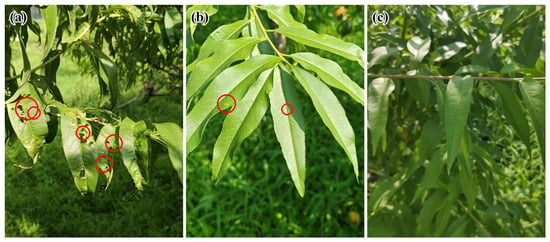
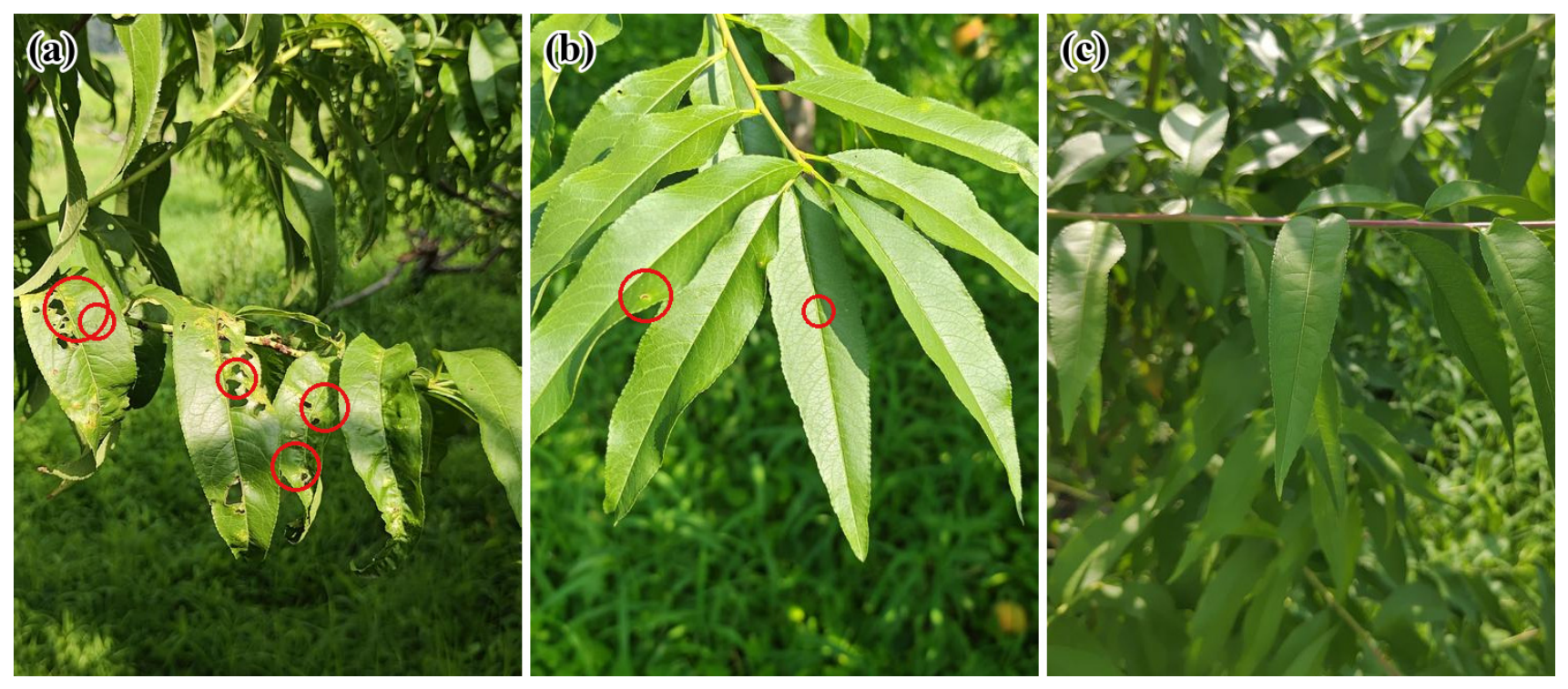
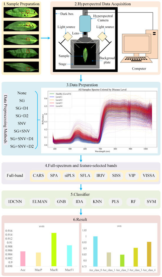
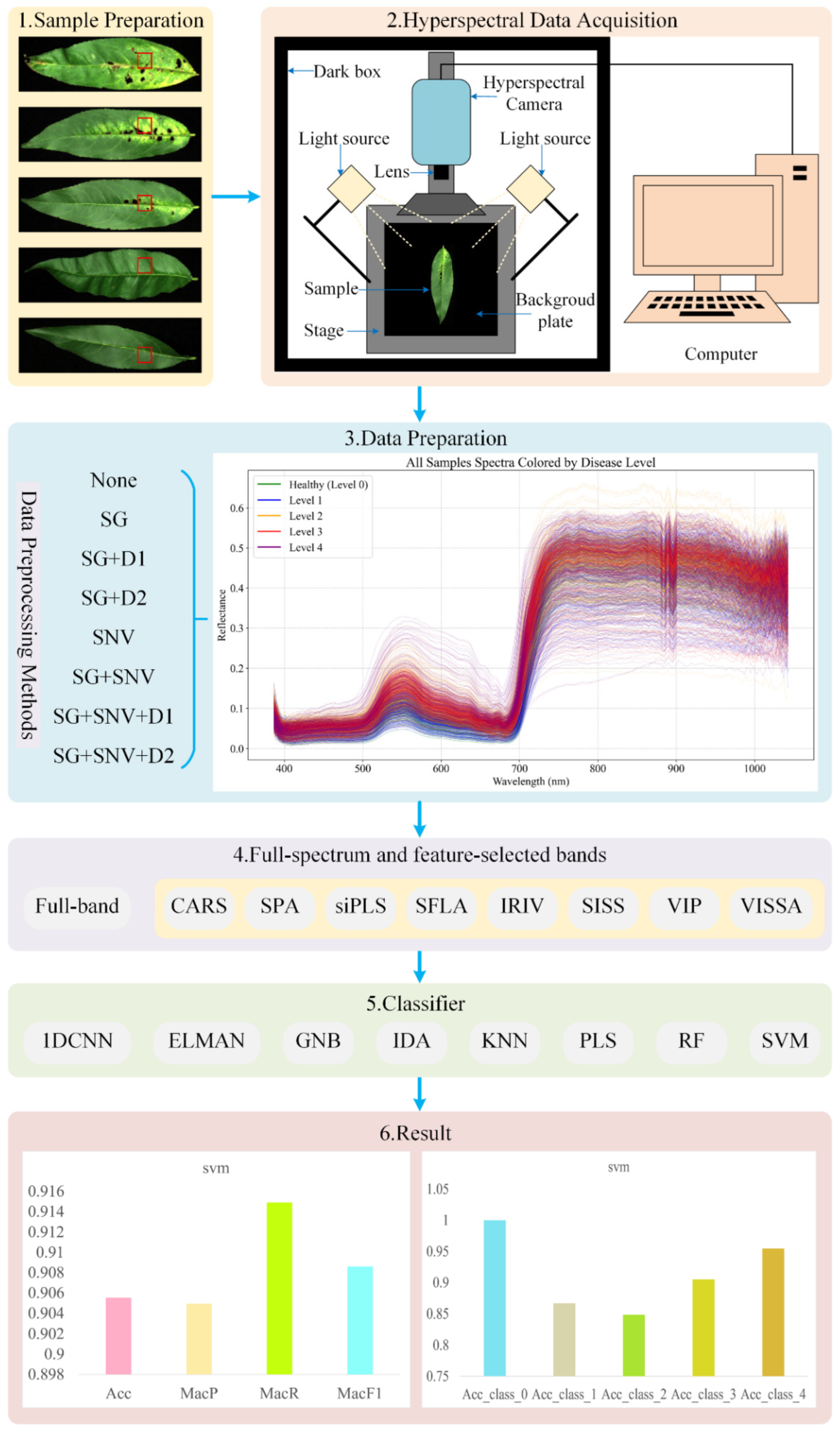
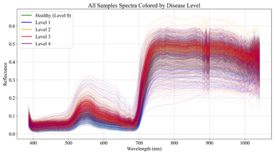
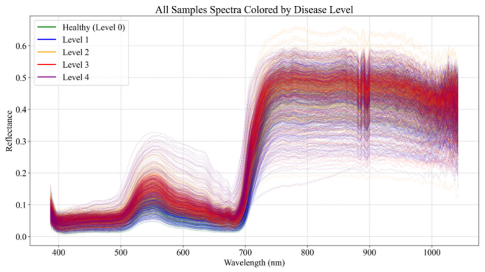
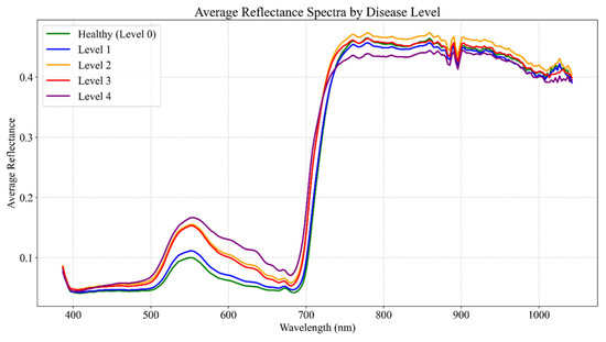
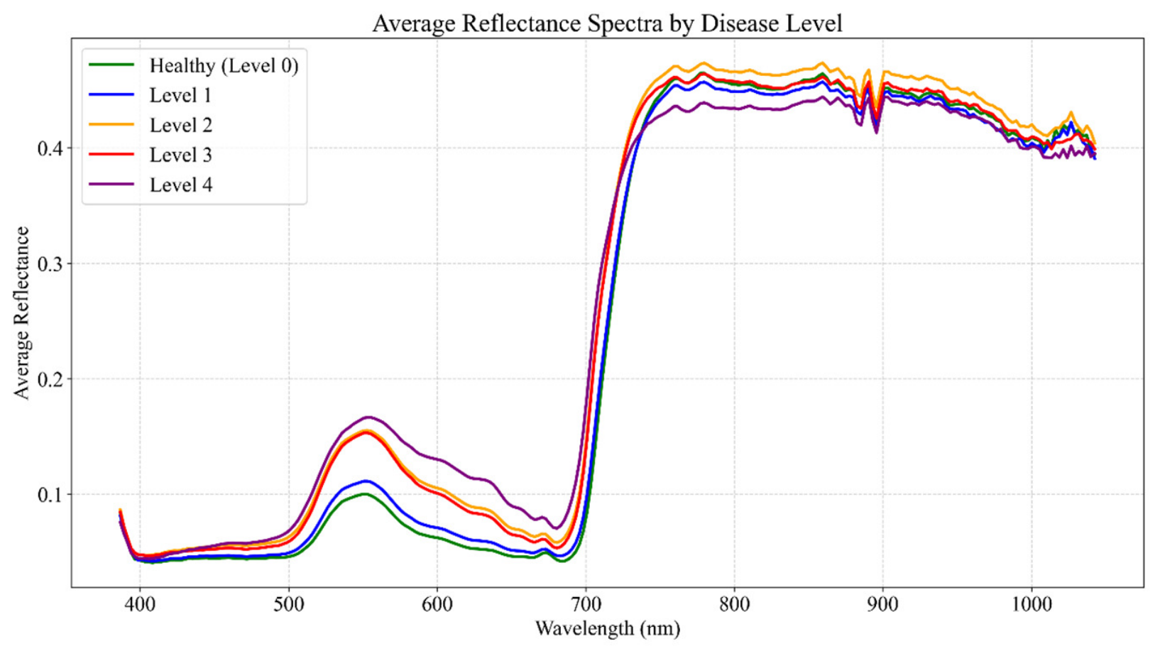
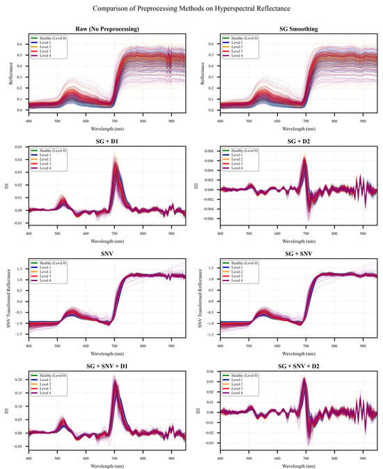
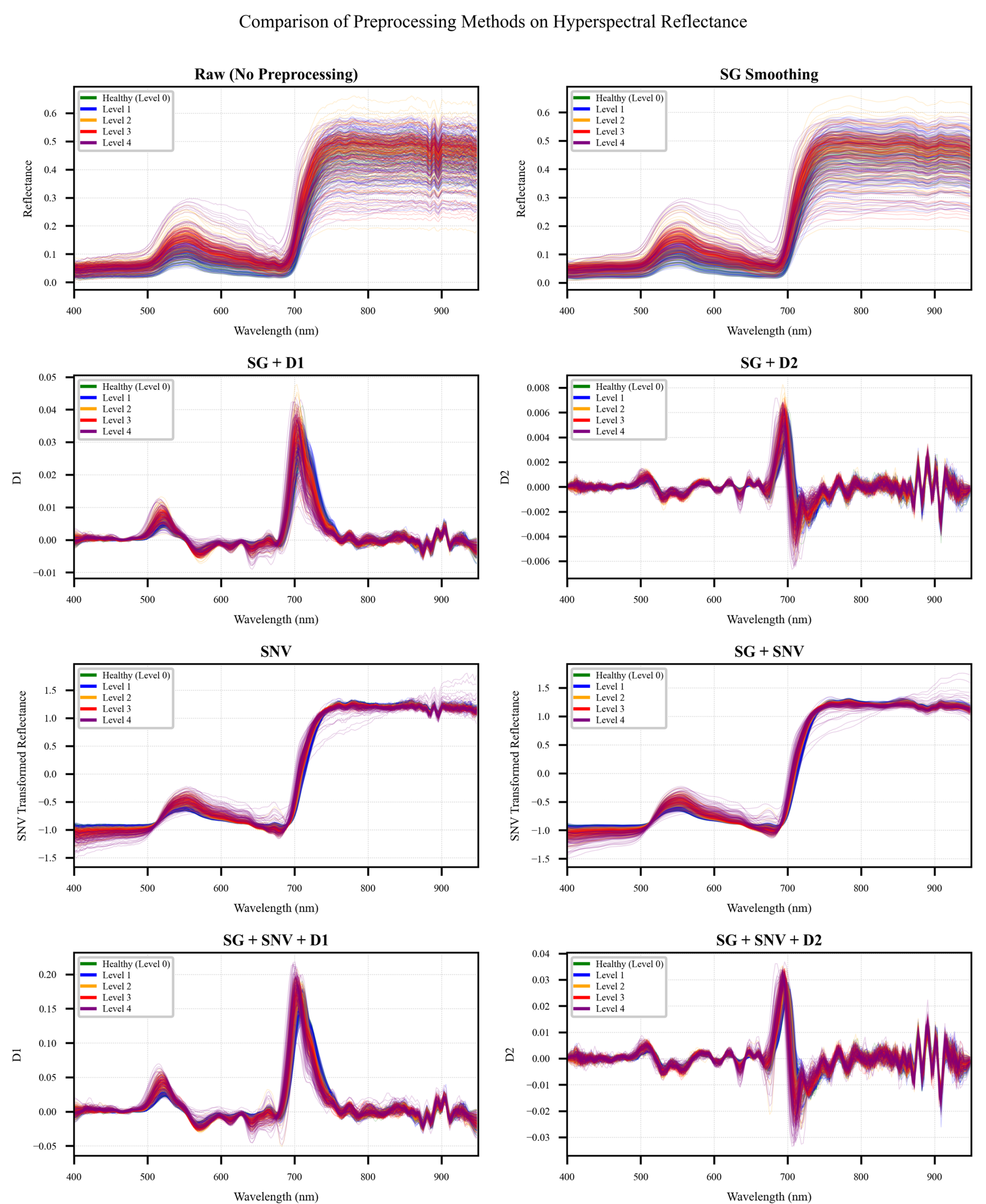
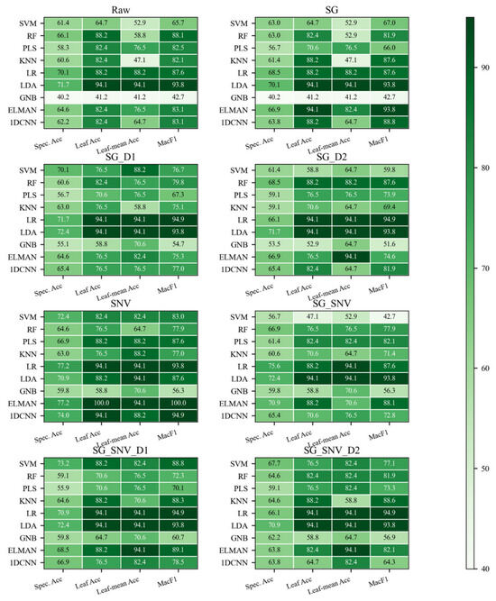
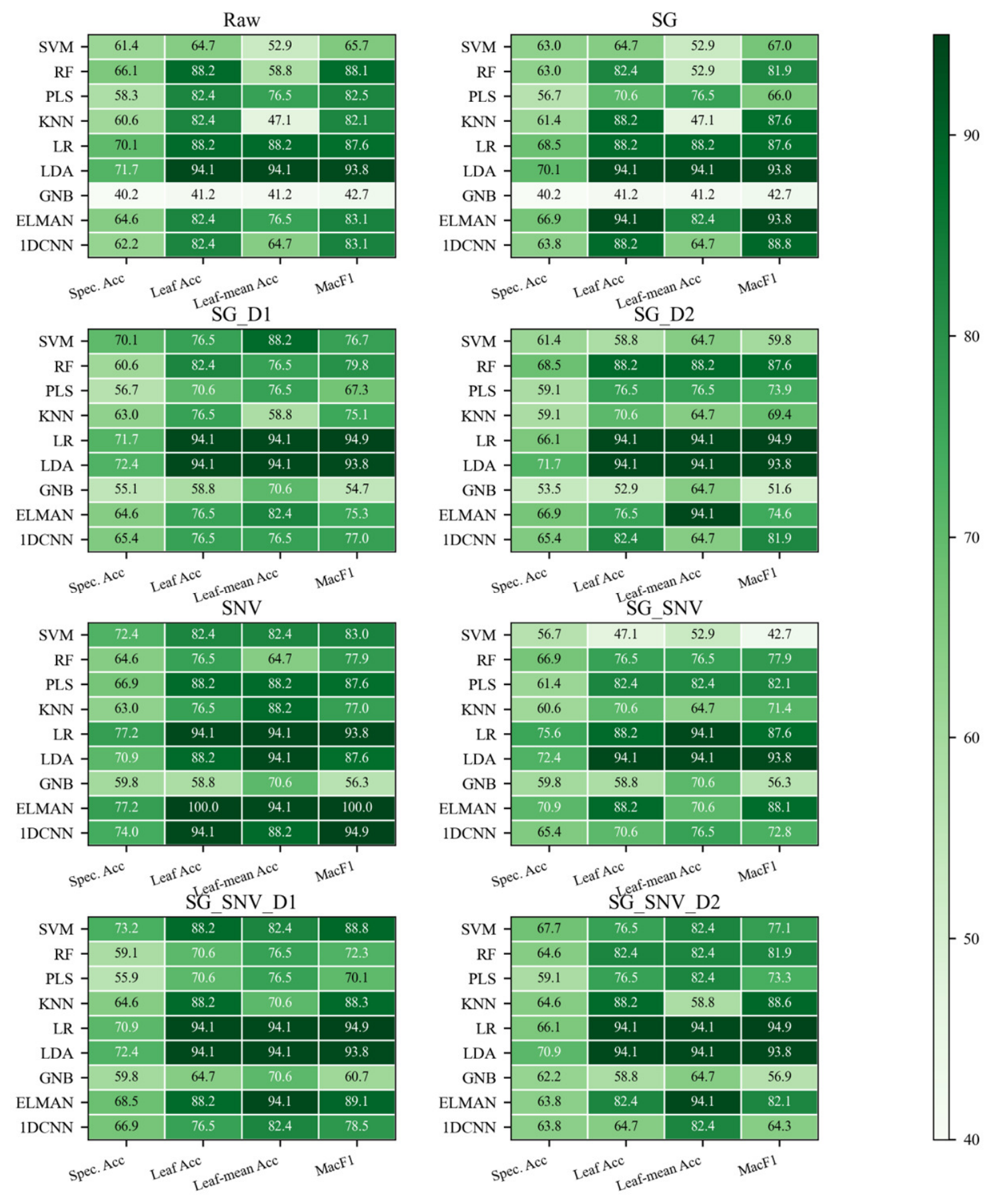
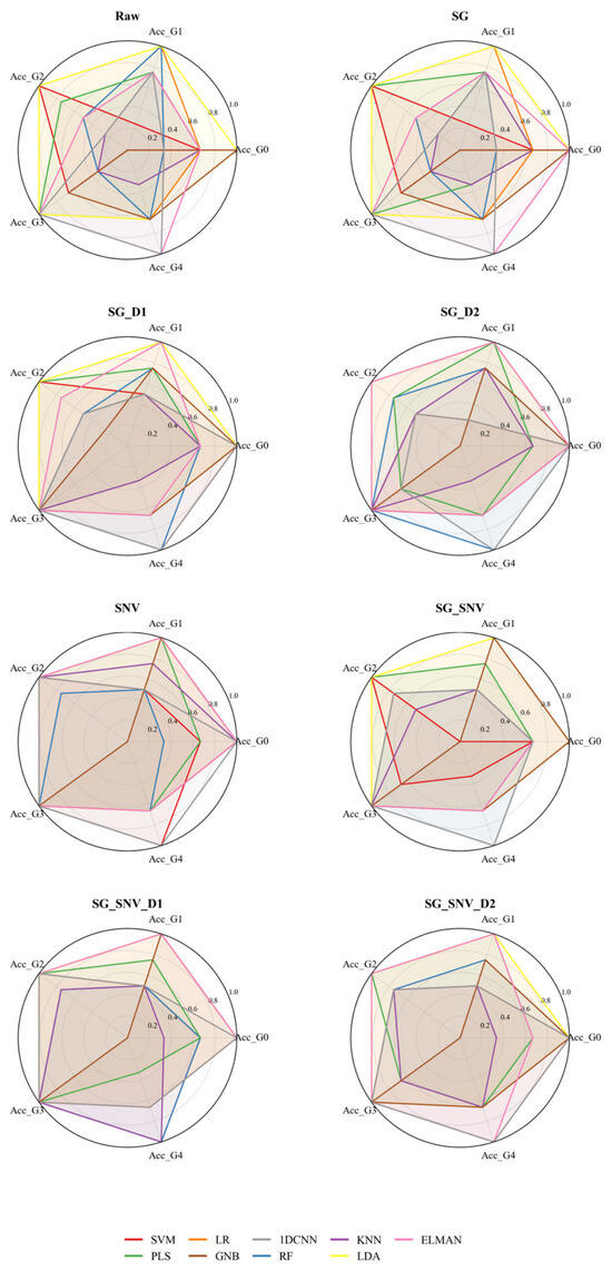
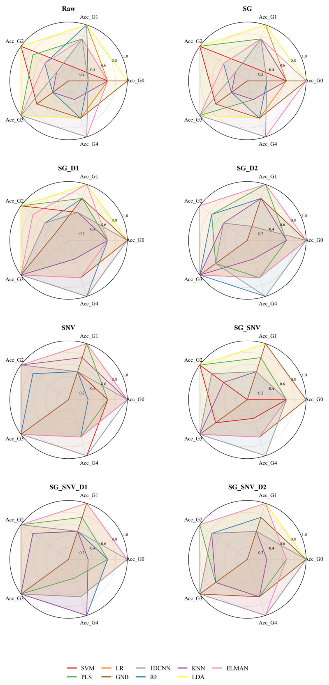
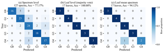
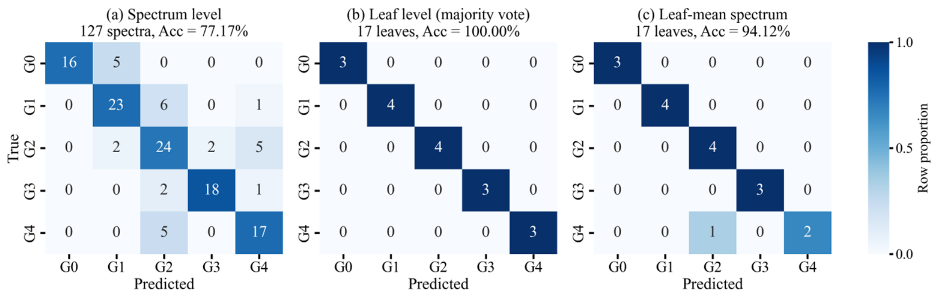
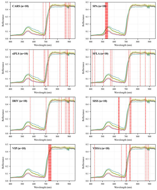
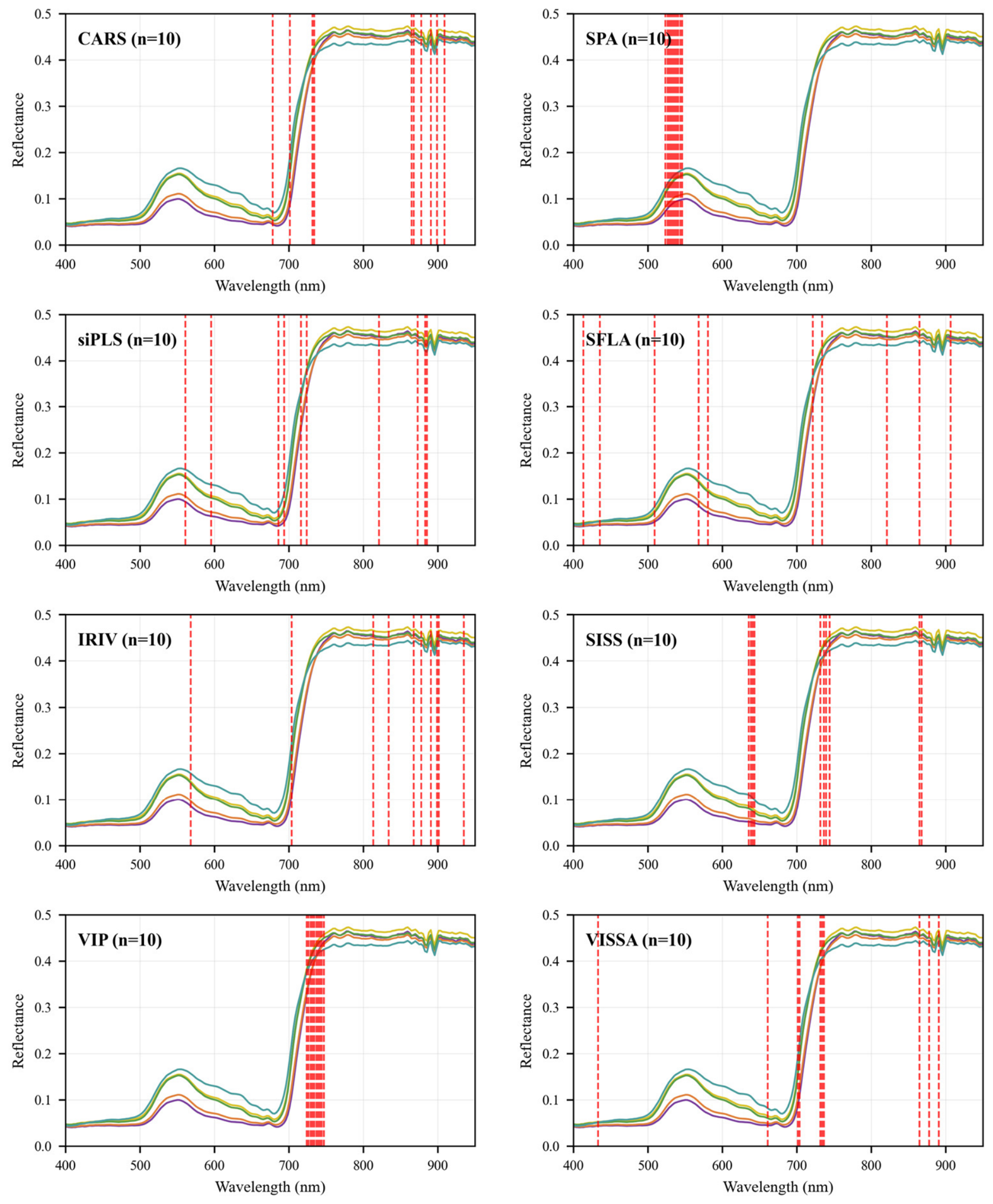
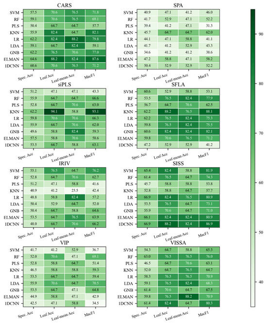
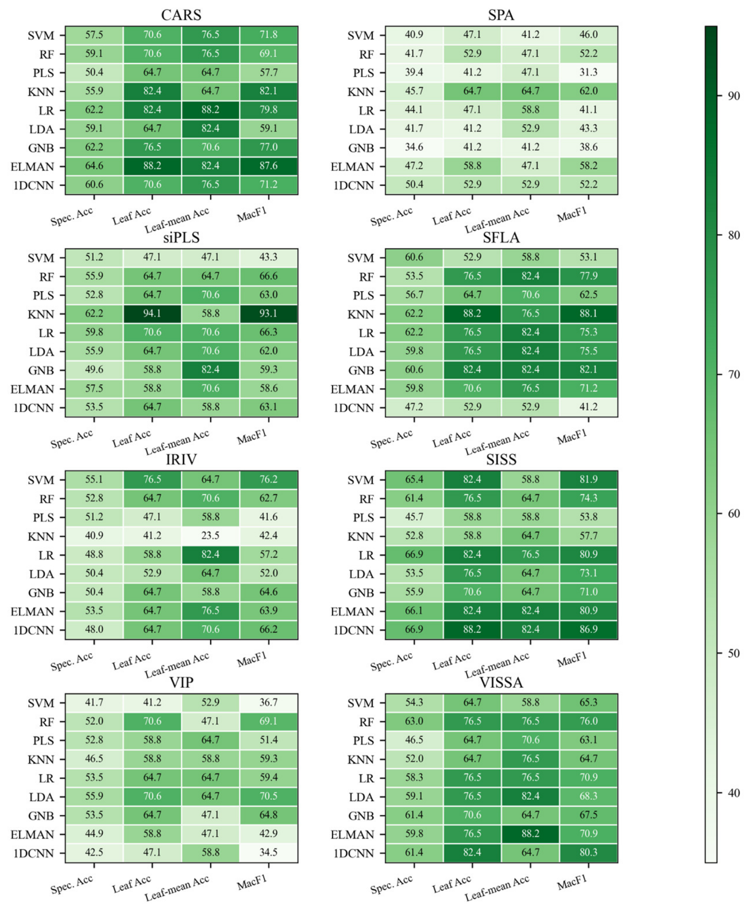
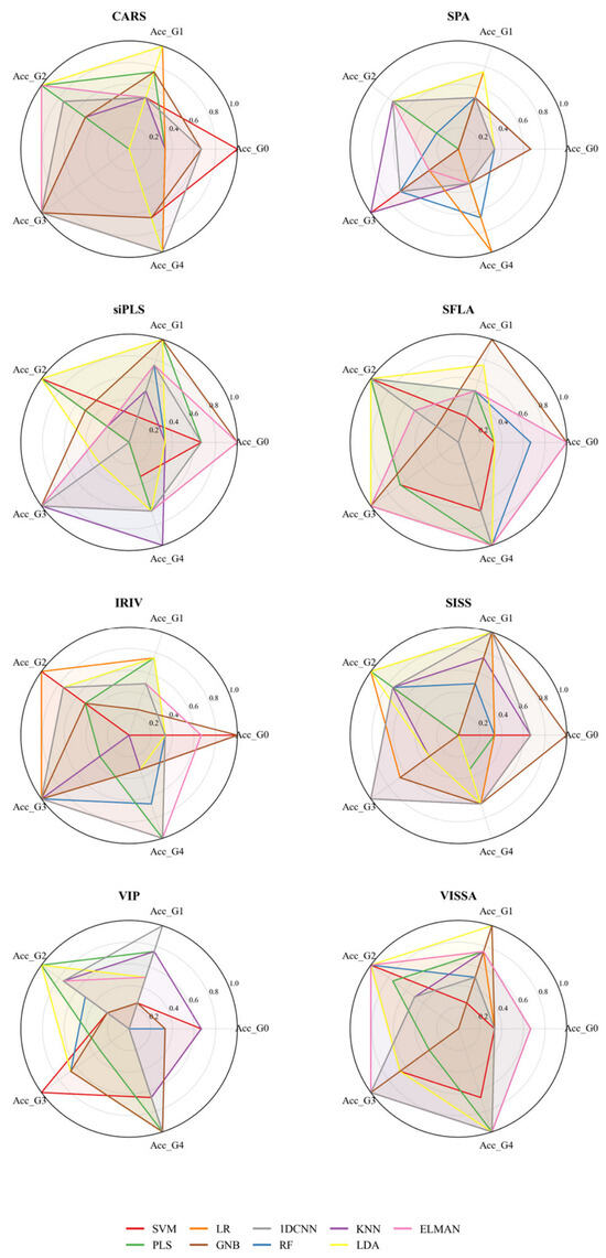
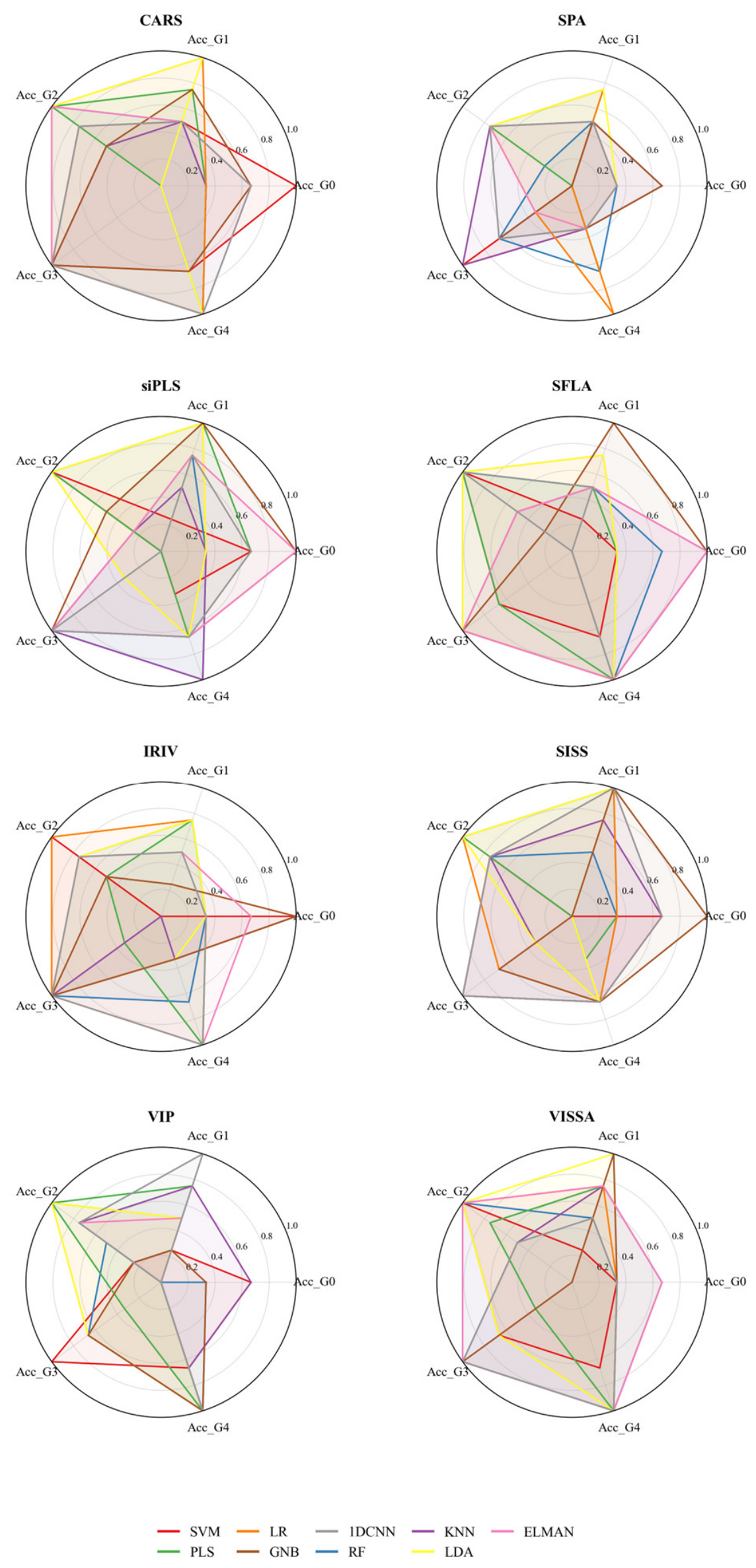

Disclaimer/Publisher’s Note: The statements, opinions and data contained in all publications are solely those of the individual author(s) and contributor(s) and not of MDPI and/or the editor(s). MDPI and/or the editor(s) disclaim responsibility for any injury to people or property resulting from any ideas, methods, instructions or products referred to in the content. |
© 2026 by the authors. Licensee MDPI, Basel, Switzerland. This article is an open access article distributed under the terms and conditions of the Creative Commons Attribution (CC BY) license.