Analysis of Tractive Performance Under Multiple Operating Conditions in the Tire–Soil Interaction

Abstract

Aiming to analyze the tractive performance of a 6.00-14 bias-ply tire with a chevron tread pattern on soil, we conducted experiments to measure the influencing factors and calculated the Mohr–Coulomb-based traction-related index coefficient using traction theory. The influencing factors considered in this study included soil cohesion, dynamic load, contact area between the soil and tire, and soil internal friction angle. A soil bin testing facility and a laser profiler were used to measure the soil–tire coupling parameters, and an unsaturated soil stress–strain controlled triaxial apparatus was used to determine soil cohesion and internal friction angle based on the Mohr–Coulomb failure criterion. The results indicate that tire inflation pressure exerts the most significant influence on tractive performance, followed by tire load, while forward speed shows a relatively minor effect. The interaction between inflation pressure and load significantly affects soil–tire coupling parameters, whereas interactions involving speed are not significant. The combination of low tire load, low inflation pressure, and high forward speed (W = 1.5 kN, p_i = 138 kPa, S = 3 m/s) led to the maximum Mohr–Coulomb-based traction-related index coefficient among all tested conditions. This study includes tire–soil contact properties for low-ground-pressure tire technologies, precision tire inflation pressure, and forward speed management, for better traction and reduced soil compaction.

1. Introduction

Agricultural tractors are used in many aspects of agricultural production, such as tillage, seeding, and harvest, as they are equipped with drive wheels [1,2,3]. Tractor power output, including hydraulics, makes tractors an important power source for many types of agricultural machinery [4]. Tractors and their implements, as well as combines, represent a larger sector of agricultural equipment manufacturing.

The use of agricultural tractors is increasing worldwide. The tractor market is estimated to rise from USD 70.40 billion in 2024 to USD 90.71 billion in 2029 at a compound annual growth rate (CAGR) of 5.2%. The performance of tractors directly affects agricultural productivity [5,6]. One of the representative performance indicators of tractors is traction [7]. In the field of terramechanics, the driving and traction performances of off-road vehicles, including tractors, operating on soil have been evaluated, and their importance has been emphasized [8]. The tractive performance of a wheeled tractor affects drawbar pull applied to the implement as well as operational efficiency and fuel consumption [9]. For high-draft implements, most of the traction force is used to wing the attached implement and overcome motion resistance [10]. So, the traction performance of a wheeled tractor is highly dependent on the soil condition, tire slip, tractor specifications, dynamic load on the tires, tire type, and tire inflation pressure [11,12,13,14]. The ability to predict and optimize the performance of these tractors during field operations has been of great interest to scientists, manufacturers, and users.

To predict tractor performance and achieve optimized tractive efficiency, it is necessary to develop predictive equations and the parameters contained in the equations should be obtained easily. Over the last few decades, to quantify the soil–machine interaction, a large number of studies have been conducted. These attempts can be classified under the following three broad categories: (1) analytical methods; (2) semi-empirical, parametric, or analog methods; and (3) empirical methods [15].

The theoretical approach is very appealing and elegant [16,17]. The geometry of the 3-D contact surface and the stress distribution at the soil–tire interface have been the basic unknown quantities used to predict the performance of a traction device. Some researchers have predicted traction performance based on passive pressure theory or plasticity theory. Finite Element Models (FEMs) have been used in some prediction models, since FEMs are particularly suitable for investigating complex problems involving geometric and material nonlinearities [18,19,20]. However, the complexity of the problem and the need for numerous soil parameters restricted the development of applying FEMs to soi–tire interaction. The interaction between the soil and the traction device, represented by two simulators (a flat plate and a torsional shear device or a rectangular grouser unit) [21], is a typical application of semi-empirical and parametric methods. Generally, only necessary soil parameters have been obtained, using a device known as a bevameter [22]. Bekker established an equation for the normal stress under a flat plate, and Wong [23] and Moro [24] used this equation or modifications thereof to determine rolling resistance due to the deformation of soil by a traction device. The empirical approach is intended for quick numerical evaluation of soil in the field. Wulfsohn [15] and Upadhyaya et al. [21] established a prediction equation with 13 parameters, and conducted more than 1500 experiments to obtain these parameters. Upadhyaya et al. [22] claimed that these empirical models possess superior predictive ability.

Some new technologies, such as digital twin technology, have also been used in research on soil–tire interaction. Venturini et al. [25] developed a digital twin of a tire–rim system under biaxial loading conditions and validated the model through numerical–experimental comparisons of camber angle and stress responses. Martelli et al. [26] developed a digital-twin-oriented dynamic simulation framework for agricultural tractors by integrating vehicle dynamics, powertrain characteristics, and tire–soil interaction models to evaluate traction performance under soft-soil farming conditions. Guo et al. [27] developed a digital-twin-assisted online optimization method for adjustable parameters of agricultural machinery and applied it to optimize the operating settings of a corn combine harvester. However, all these models were established on a computer and did not have any corresponding field experiments to support them.

Control of the performance characteristics of a single wheel is typically better than that attainable when studying the wheels of a test vehicle. Tire performance characteristics include forward velocity, wheel angular velocity, slip, tire inflation pressure, tire steer angle, and dynamic load. Thus, a single wheel mounted to a soil bin test carriage that operates on fixed guide rails was a good choice for investigating traction performance.

In this study, we chose the empirical method and used a single tire with a chevron tread pattern on soil to conduct the experiment and calculate the Mohr–Coulomb-based traction-related index coefficient. This development includes tire-rigid surface and tire–soil contact properties for low-ground-pressure tire technologies, precision tire inflation pressure, and forward speed management, for better traction and reduced soil compaction. The main contribution of this study is a controlled single-wheel soil-bin experiment that jointly evaluates the main and two-factor interaction effects of tire inflation pressure, vertical load, and forward speed on post-pass rut geometry and topsoil stress responses. Soil mechanical parameters obtained from triaxial testing are further used to derive a Mohr–Coulomb-based traction-related index for auxiliary, within-study comparison. The objectives of this study are to:

(1) Investigate the effects of soil cohesion, dynamic load, contact area between the soil and tire, and the soil’s internal friction angle on the Mohr–Coulomb-based traction-related index coefficient.

(2) Investigate the effects of tire–soil contact properties for low-ground-pressure tire technologies, precision tire inflation pressure, and forward speed management, for better traction and reduced soil compaction.

2. Materials and Methods

2.1. Experiment Materials

2.1.1. Soil Samples

The experiment was conducted on a clay loam soil in the soil bin (21.67% sand, 35.89% silt, and 42.44% clay). Soil texture was classified according to the United States Department of Agriculture (USDA) soil textural classification system. The test soil was directly obtained from the field, with the sampling location in the Jiangsu Experimental Farm of Nanjing Agricultural University area of Nanjing, China. Using specialized tools (an undisturbed soil sampler), the field soil was collected in its “original state” while preserving its natural layers, and then placed into the soil bin. Under these conditions, the test soil retains as much as possible its original physical structure. The mean physical properties of the untrafficked soil are presented in Table 1.

Table 1. Mean physical properties of untrafficked soil.

Depth (cm)	Mean Dry Bulk Density (g/cm3) a	Mean Soil Moisture Content (Wet Basis) w (%)	Soil Mechanical Composition (%)			Mean Soil Cone Index (kPa)
						Depth
			Clay <0.002 mm	Silt 0.002–0.05 mm	Sand >0.05 mm	100 mm	200 mm	300 mm
0–5	1.29	17.65	21.67	35.89	42.44	21	177	414

Note: “a” Cylindrical soil cores, 30.9 mm diameter × 20 mm height.

2.1.2. Soil Cone Index

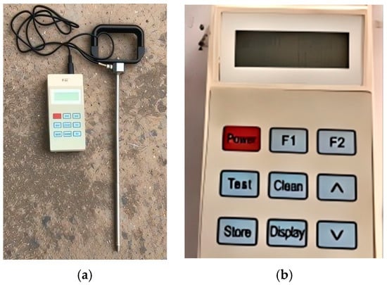
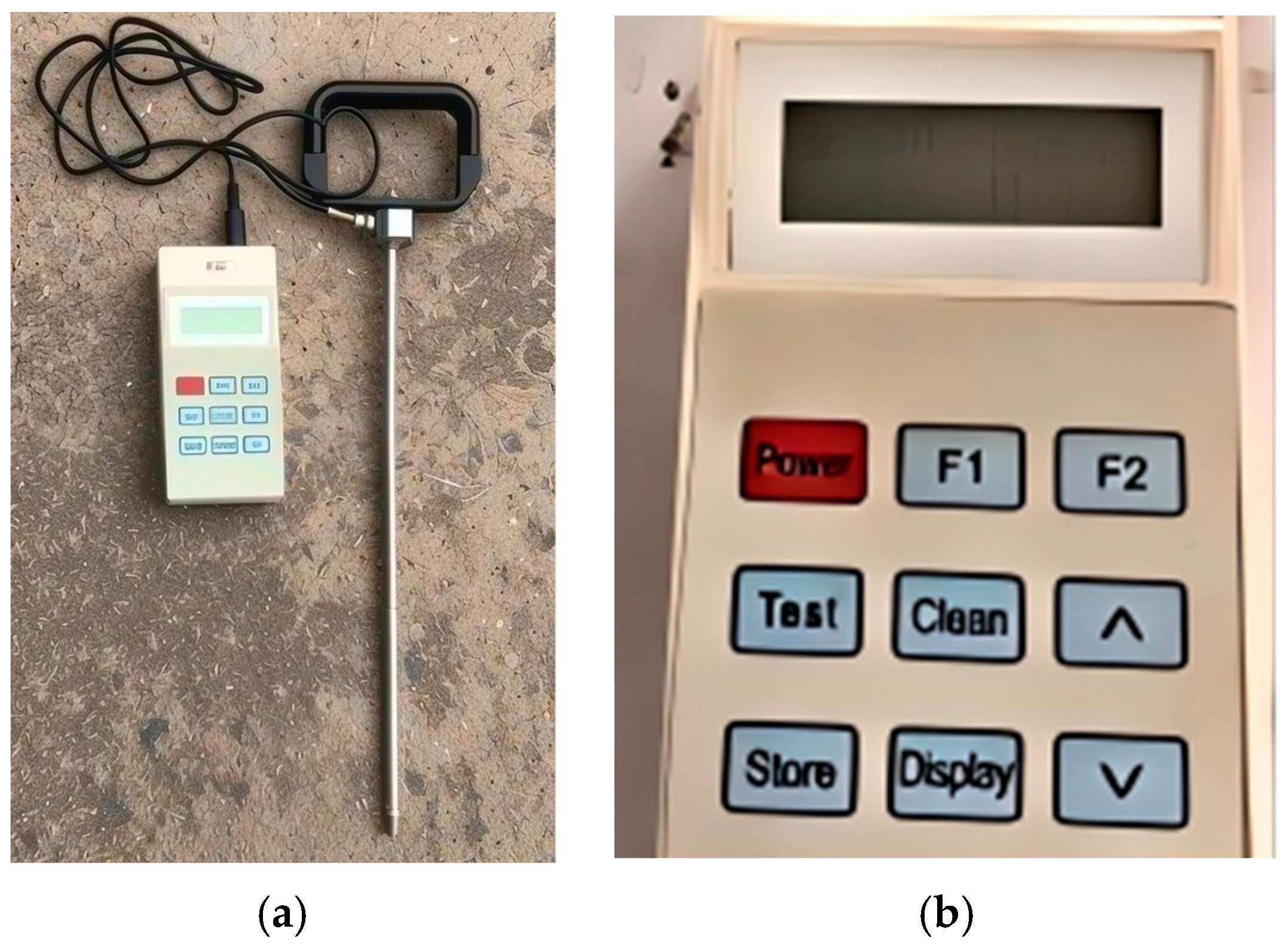
A soil cone penetrometer (Figure 1) (model TJSD-750, Zhejiang Top Instrument Co., Ltd., Hangzhou, China), with a measurement range of 0–7000 kPa, was used to measure the soil compactness, from which the soil cone index could be calculated. The precision of the soil cone penetration resistance measurements was ±1% of the full-scale penetration resistance, and the measurement depth range was 0–450 mm. The location of each cone penetration was determined from GPS coordinates, and a soil compactness distribution map could be developed based on the location data.

Figure 1. Soil compactness meter and control panel. (a) Soil compachtmess; (b) Control panel of the soil compactness meter.

2.1.3. Soil Bin Testing Facility

The vehicle engineering laboratory of Nanjing Agriculture University developed the soil bin testing facility (Figure 2), which was used for the experiments. The size of the soil bin was 9 m × 1.5 m × 0.8 m (length × width × depth) [28]. The components of the soil bin system include a towing system, a driving system, the soil bin, a control system, and a data acquisition system.

Figure 2. Top view of soil bin testing facility. 1—Torque and speed sensors for drag motor; 2—Drag motor; 3—Vertical guide bearing; 4—Wheel driving motor; 5—Test tire; 6—Single tire tester; 7—Drive torque sensor and speed sensor; 8—Driving mechanism base plate; 9—Guide rail; 10—Soil; 11—Drag chain; 12—Pressure sensors in the soil were at this general location relative to the approaching tire; 13—The vertical displacement sensor was mounted on the driving backplane, and measured the distance between the soil and the driving backplane.

A single tire tester on the soil bin was equipped with a 6.00-14 bias-ply agricultural drive tire, with a lug height of 20 mm measured at the tire central plane. The tire overall diameter was 673 mm, the tire section width was 153 mm, and the half-width contained 18 lugs. The driving motor provided driving torque to the wheel of the test tire. When the tire developed positive net traction, the forward motion of the single tire tester was resisted by the drag chain, whose motion was resisted by the drag motor.

A vertical displacement sensor was mounted on the driving mechanism base plate and measured the distance between the soil and the driving mechanism base plate. An array of 18 pressure sensors, buried in the topsoil, measured vertical soil pressures beneath the tire. Data from the vertical displacement sensor, the 18 soil pressure sensors, a torque sensor measuring torque applied to the wheel of the test tire, and a wheel forward speed sensor for the test tire were acquired by a data acquisition system. The single tire tester was able to control the tire vertical load, the net traction developed by the tire, and the tire forward velocity.

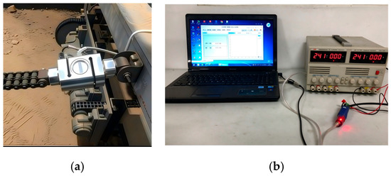
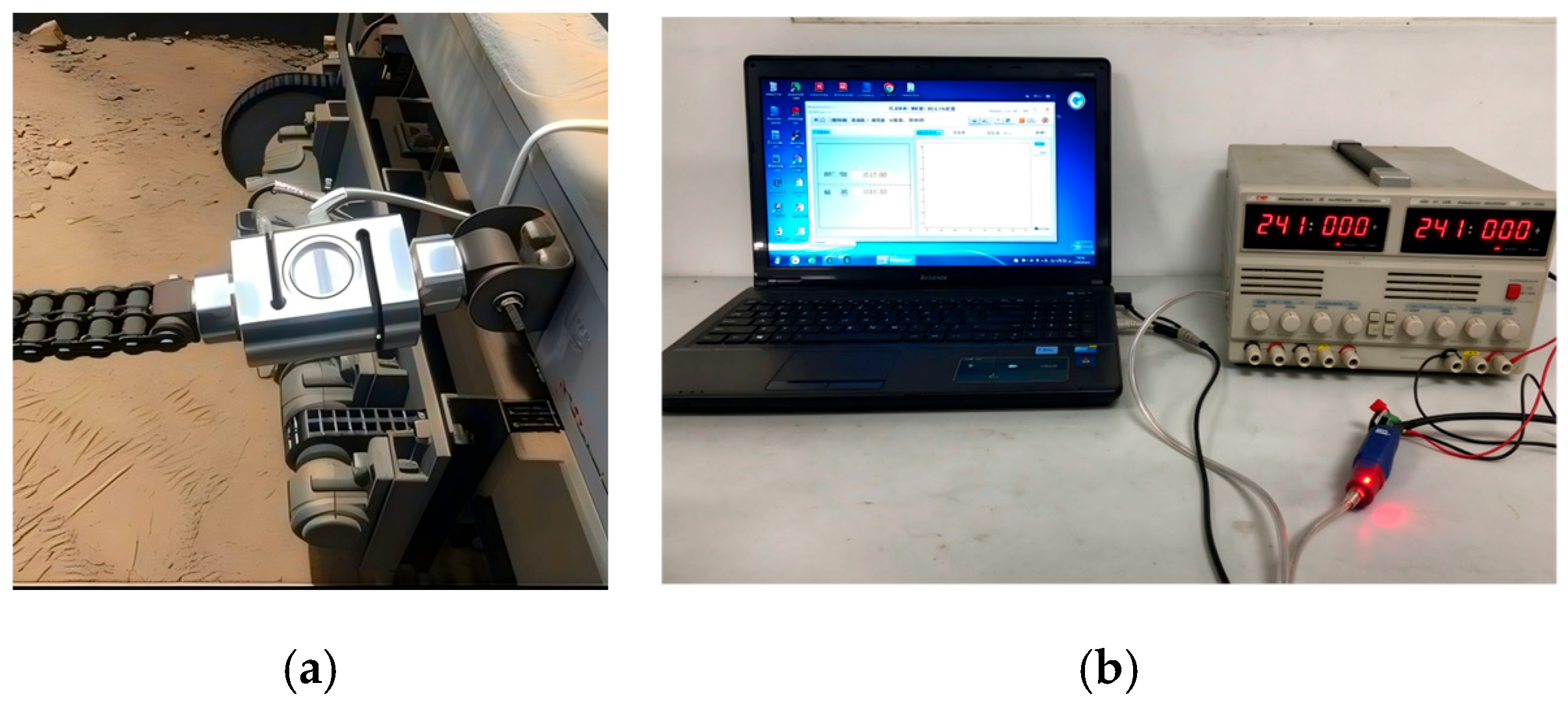
Figure 3 shows the traction test system. During the experiment, a pull pressure sensor (model JLBZ, Bengbu Jinnuo Sensor Co., Ltd., Bengbu, China) (Figure 3a) was mounted in the drag chain of the soil bin testing facility to measure the traction of the single tire. A matching transducer (model BSQ-DG1, Bengbu Jinnuo Sensor Co., Ltd., Bengbu, China) was used for signal transformation, and the connection type is shown in Figure 3b. We measured the traction force of the tire under forward speeds, tire vertical loads, and tire inflation pressures.

Figure 3. Load cell of the traction test system. (a) pull pressure sensor; (b) connection type.

2.1.4. Soil Vertical Stress Measurement System

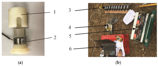
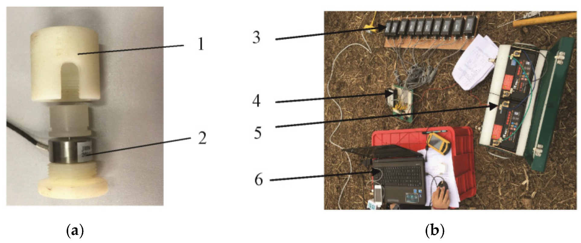
The components for measuring the vertical stress in soil consisted of stress sensors, an amplifier, a power supply, a data acquisition card, and a computer. The transducer within each stress sensor (Figure 4a) was a model JHBM 50 kg capacity miniature load cell (Luoyang Bader E-commerce Co., Ltd., Xigong District, Luoyang, China). The cylindrical, alloy steel load cell has a diameter of 15 mm diameter and a thickness of 10 mm, and the precision was ±0.05% of full-scale force capacity. To protect the load cell, a nylon protective cover with a height of 30 mm and a diameter of 30 mm [28] housed the load cell. The load cell output voltage of the stress signal was amplified by a BAQ-JN amplifier (Bengbu Sensor System Engineering Co., Bengbu, China) to 0 to 5 V. The vertical stress range for the stress sensor was 0 to 708 kPa, and the data collected by components of the stress sensor system are shown in Figure 4b.

Figure 4. The test system of stress sensors. Legend: (a) Stress sensors and protection cover; (b) Test system. Legend: “1”—Protection cover; “2”—Stress sensor; “3”—Amplifier; “4”—Data acquisition card; “5”—Power; “6”—Computer.

2.1.5. Soil Rutting Measurement Instrument

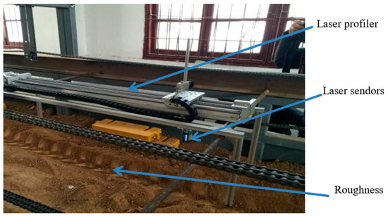
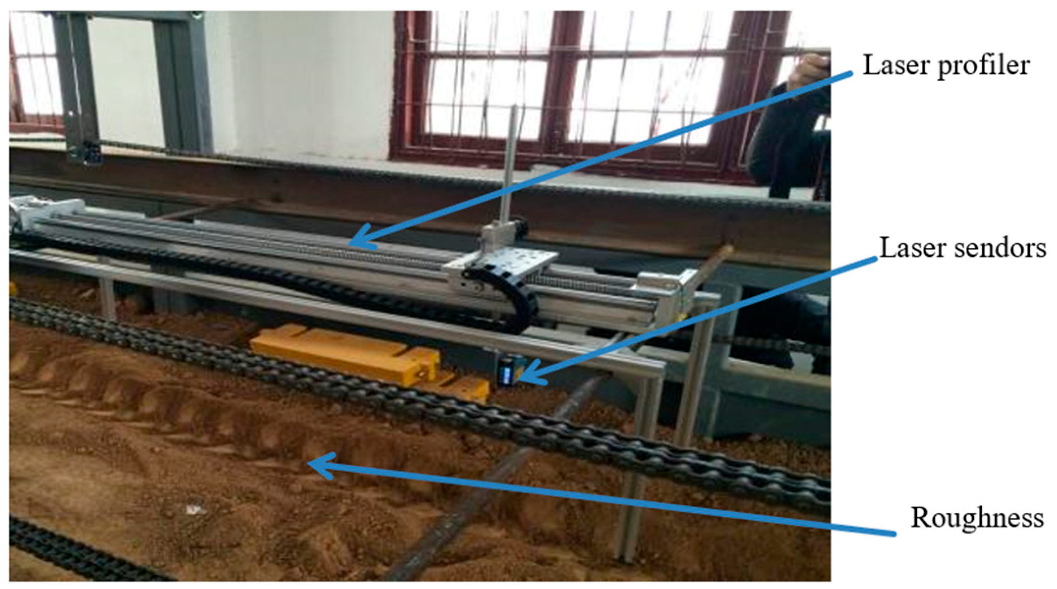
A SICK DT20-P214B laser distance sensor (SICK China Co., Ltd., Guangzhou, China) was used to measure the vertical distance between the laser sensor and the soil surface. The laser sensor was mounted on a laser profiler. The longitudinal scanned length was 1 m, the precision of the laser profiler was ±0.5 mm, and the sampling interval along the longitudinal direction was 5 mm. The sampling interval along the lateral direction was 10 mm. After the tire formed a soil rut, we made one scan along the tire central plane and eight longitudinal scans on each side of the central plane scan, with a total of 17 scans, to describe the roughness after rutting in each combination of tire load, inflation pressure, and forward speed. Soil rut measurements were made for various tire loads, tire inflation pressures, and forward speeds, but with the same soil condition. Figure 5 shows the positioning of the laser profiler for measuring a soil rut.

Figure 5. Measurement of roughness by laser profiler.

The laser profiler was used to measure the vertical distance at each measurement location, relative to the undisturbed soil surface. Furthermore, all the contact areas in this study were derived from laser-profiler-based reconstruction of rut surfaces after tire passage, representing geometric features of the post-rolling rut instead of the instantaneous real contact area between tire and soil.

2.2. Experimental Methods

2.2.1. Measurement of Soil Cohesion and Soil Internal Friction Angle

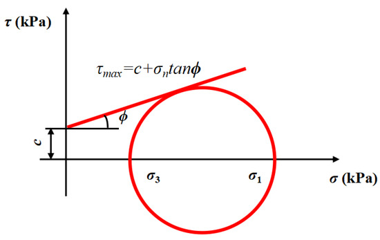
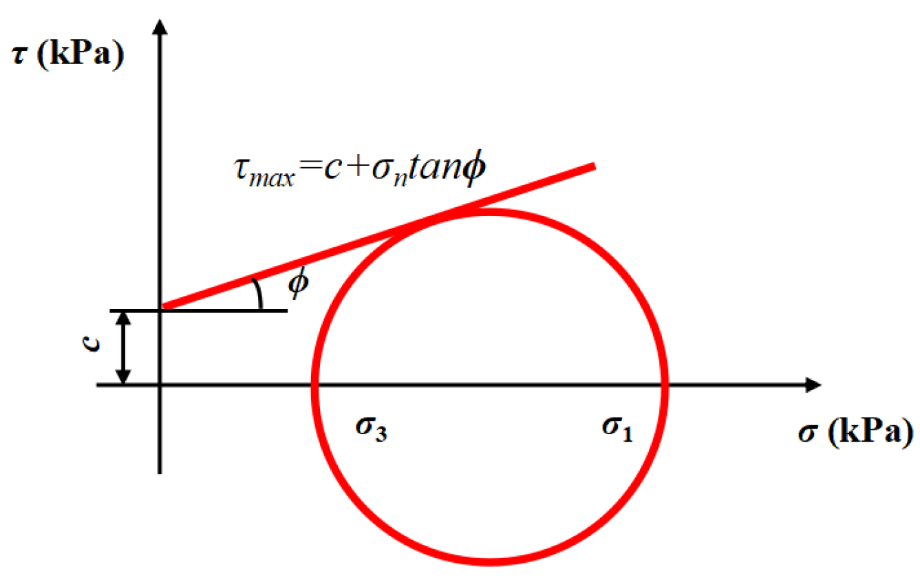
As shown in Figure 6, Mohr’s circle was used to express the soil stress limit, and the line named the Coulomb line was used to express the soil shear strength. Based on the Mohr–Coulomb failure criterion-limit equilibrium state, when the Coulomb line was tangent to Mohr’s circle, the shear strength of soft soil reached the limit. The radius of the Mohr’s circle equals (σ₁ − σ₃)/2 and the distance between the center of the Mohr’s circle and the Y-axis is (σ₁ + σ₃)/2, where σ₁ and σ₃ are the major principal stress and minor principal stress, respectively. The intercept, c, is the soil cohesion, and the inclination angle, Ø, is the soil internal friction angle.

Figure 6. Mohr–Coulomb failure criterion-limit equilibrium state.

We know that σ₁ ≥ σ₃, and the maximum shear stress can be described as:

$$({\sigma }_1-{\sigma }_3)/2=c·\mathrm{c}\mathrm{o}\mathrm{s}Ø+\mathrm{s}\mathrm{i}\mathrm{n}Ø \ast ({\sigma }_1+{\sigma }_3)/2$$

(1)

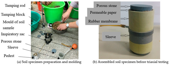
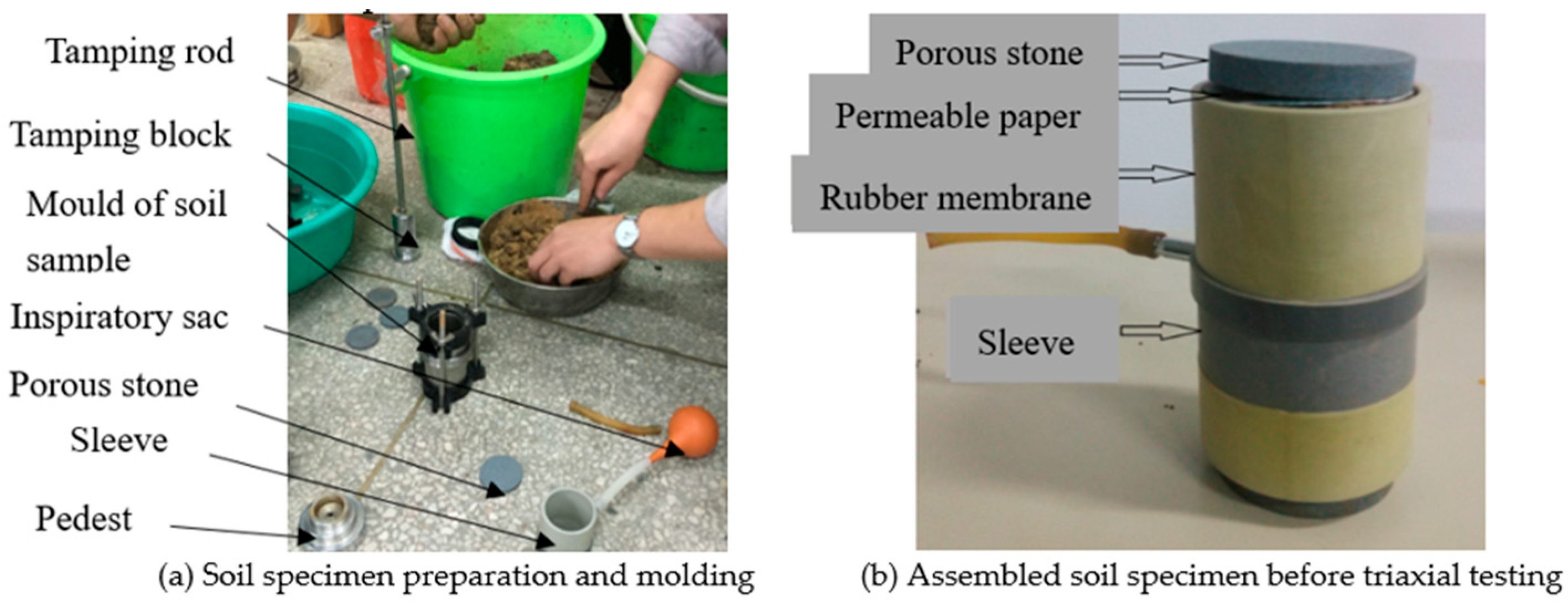
To obtain σ₁ and σ₃, an unsaturated soil stress–strain control triaxial instrument, model TFB-1 (Road Instrument Branch Nanjing Instrument Factory CO. LED, Nanjing, China), was used. In accordance with GB/T 50123-2019 [29], four soil samples were prepared with a size of 61.8 × 125 mm (diameter × height). All the soil samples were collected from the soil bin.

Figure 7a shows the process of making soil samples, and Figure 7b shows the complete soil samples.

Figure 7. Soil sample preparation.

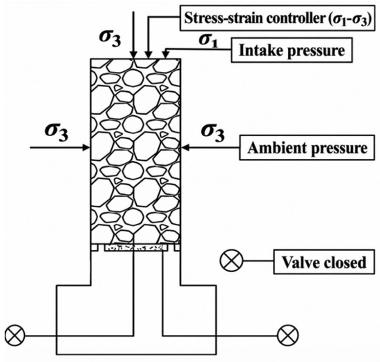
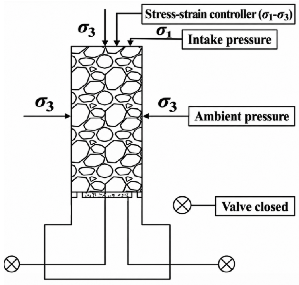
The prepared soil sample was sealed with rubber film to prevent water from entering the soil sample and then installed on the base of the triaxial apparatus. The outer chamber under water pressure was installed, and a displacement sensor on the top was moved to contact the top of the pressure chamber to measure the soil axial strain. After the soil sample was installed, the experiment of measuring the soil shear strength was conducted based on the unconsolidated–undrained shear test (UU test) (Figure 8).

Figure 8. Unconsolidated–undrained test of unsaturated soil using a triaxial apparatus. The ambient pressure (σ3) and principal stress difference (σ₁ − σ₃) were set before the experiment. The stress–strain controller was used to control the value of the principal stress difference (σ₁ − σ₃).

The initial value of the ambient pressure applied to the soil sample was set at 40 kPa, and the soil sample was sheared at a constant strain rate (1 mm/min) until the axial strain reached about 4%. The value of ambient pressure was then increased to 80 kPa, and the soil sample was sheared with the same strain rate (1 mm/min) until the axial strain reached about 8%. The value of ambient pressure was then increased to 120 kPa, and the soil sample was sheared with the same strain rate (1 mm/min) until the axial strain reached about 12%, which reached the termination conditions of the experiment, and then the ambient pressure was uninstalled. The data were recorded when the sample resulted in an axial deformation of 0.1 mm.

For each soil sample, we determined the values of (σ₁ + σ₃)/2 and (σ₁ − σ₃)/2, and drew the diagram of the Mohr–Coulomb failure criterion-limit equilibrium state. Another three soil samples were conducted in the same experiment so that four different values of tthesoil adhesion coefficient and soil internal friction angle could be obtained, and the average of these four values was used as the final values of the soil adhesion coefficient and soil internal friction angle.

2.2.2. Data Acquisition and Processing

The tire was driven to run, and data such as traction force (measured by the tension-pressure sensor), wheel torque (measured by the torque sensor), and wheel forward speed (measured by the wheel speed sensor) were collected synchronously through the data acquisition system. Each variable combination was tested repeatedly to reduce experimental errors. The average traction force of the orthogonal test (a total of nine experiments at different forward speeds, tire load, and inflation pressure) of the tire measured in the experiment was 1.67 kN, and this was the actual traction force.

The reserve adhesion per unit load, which is the ratio of the difference between tire adhesion and rolling resistance to the tire load of an agricultural vehicle, was used as one of the tractor traction performance indicators [30]. The deformation of the rolling resistance of the driving tire does not consume the adhesion ability between the tire and the soil. So, for 4WD tractors, the evaluation index of agricultural vehicle traction performance can be described as:

$${\mu }_g=P_{max}/W_D$$

(2)

where $P_{max}$ is the Mohr–Coulomb-based traction-related index, kN; W_D is the dynamic load, kN; and μ_g is the Mohr–Coulomb-based traction-related index coefficient, also known as the adhesion coefficient [28].

Equation (2) was used in our development of the Mohr–Coulomb-based traction-related index coefficient.

$$P_{\mathrm{m}\mathrm{a}\mathrm{x}}=cA+W_{\mathrm{D}}\tan \varnothing$$

(3)

where A is the geometric proxy area obtained by reconstructing the rut surface after tire passage, mm²; c is the soil cohesion, kPa; and $\mathrm{Ø}$ is the soil internal friction angle, °.

Here, P_max in Equation (3) is a theoretical value derived from soil shear properties, not experimentally measured traction. Furthermore, we did not consider the slip ratio and tread-relevant factors in the equation, which was inconsistent with ISO/ASABE standards. Therefore, the Mohr–Coulomb-based traction-related coefficient calculated in this study is treated as a theoretical comparative index rather than as a direct measure of experimentally measured tire traction.

Substituting Equation (3) into Equation (2), we get,

$${\mu }_g=c/P_{\mathrm{D}}+\tan \varnothing$$

(4)

where $P_D={\displaystyle \frac{W_D}{A}}$ is the average vertical load per unit area.

Based on Equation (4), ${\mu }_g$ is a calculated traction-related coefficient derived from the Mohr–Coulomb soil shear-strength parameters, the applied vertical load, and the geometric area used in the calculation. The adhesion coefficient (μ_g) was influenced by soil cohesion, dynamic load, contact area between the soil and tire, and the soil’s internal friction angle. The dynamic load was the total vertical stress between the soil and the tire [31,32]. So, for a given soil and tire, the factors with the greatest influence on traction performance were forward speed, tire vertical load, and tire inflation pressure.

2.2.3. Soil Vertical Stress Measurement

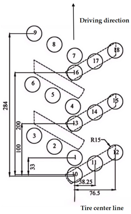
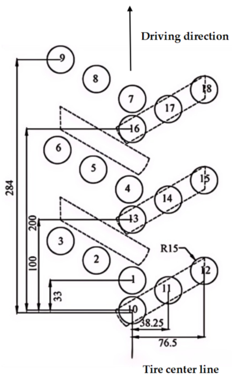
Six sensors for measuring the vertical normal soil stress were installed in the soil, at the lug right edge, lug center, lug left edge, tread right edge, tread center, and tread left edge. These six sensors, as one group of sensors, were used to study the vertical stress distribution along the lateral direction. Here, three groups of sensors, a total of 18 stress sensors, were installed in each test, and the specific arrangement scheme is shown in Figure 9. Before the installation of the stress sensors, 50 mm of topsoil was removed. The soil was placed back above the stress sensors after they were placed in the soil. Before the sensors were installed in the soil, the tire was driven once to get the tire impression. The sensors were then buried at the corresponding positions, as shown in Figure 9. However, there would still be some longitudinal motion of the tire lug relative to the sensors. To avoid this problem as much as possible, we observed whether the sensors were at the correct corresponding positions. If not, the test data were deleted, and we conducted the experiment once again until all the sensors were at the correct positions. The tractor moved forward with a particular combination of tire load, driving speed, and inflation pressure, and was stopped when the tire footprint was over the sensors. We repeated this process three times by reinstalling the sensors each time (i.e., three independent replicates), and the average value was used as the experimental result.

Figure 9. Top view of pressure sensor arrangement scheme in topsoil. Circles denote pressure sensors and dashed lines depict locations of tire lugs. Dimensions are in mm.

We assumed that the vertical stress distribution of the tire along both sides of the tire centerline was symmetrical, and then 30 data points were formed. The vertical stress in the topsoil was measured at different tire loads, tire inflation pressures, and forward speeds, resulting in 27 tests.

2.2.4. Fractal Interpolation Theory

The random 3D fractal interpolation theory [33] was used to interpolate the original measurement data. The initial point, p₀, can be chosen at random, $p_0=p_i$, $p_i\in \left\{p_1,p_2,\dots ,\right.\left.p_n\right\}$, and the data sequence is $x_1<x_2<\dots <x_n$. The first point of iteration depends on p₀ and any set of affine functions; the second point of iteration depends on the first point and any set of affine functions, and so on, until the generated iteration point meets the requirements of subsequent finite element and simulation analysis. For example, if we choose $p_0=p_1=(x_1,y_1)$ as the initial point, the iterative process can be described as:

$$\left\{\begin{array}{c}\widehat{p_1}\in \left\{F_{2,2}\left(p_0\right)\right., F_{\mathrm{2,3}}\left(p_0\right), F_{3,2}\left(p_0\right), F_{3,3}\left(p_0\right), \dots , \left.F_{N, M}\left(p_0\right)\right\}\\ \widehat{p_2}\in \left\{F_{2,2}\left(p_1\right)\right., F_{\mathrm{2,3}}\left(p_1\right), F_{3,2}\left(p_1\right), F_{3,3}\left(p_1\right), \dots , \left.F_{N,M}\left(p_1\right)\right\}\\ ⋮\\ \widehat{p_n}\in \left\{F_{2,2}\left(p_{n-1}\right)\right., F_{\mathrm{2,3}}\left(p_{n-1}\right), F_{3,2}\left(p_{n-1}\right), F_{3,3}\left(p_{n-1}\right), \dots , \left.F_{N,M}\left(p_{n-1}\right)\right\}\end{array}\right.$$

(5)

where $\widehat{p_n}(n=1,2,3,\dots )$ is the basic interpolation data point, and F_N,M (N = 2, 3, …, N, M = 1, 2, …, M) is the test point. If N′ is the total number of iterations, then the point set $\left\{(x_n,y_n|n =1,2,\dots ,N^{\prime }\right\}$ is all the reconstructed data points.

In the implementation, the initial point $p_0$ was randomly selected from the original measured points, and one admissible affine function was selected with equal probability at each iteration. The iteration was terminated when the predefined number of reconstructed points, N′, was reached. The same interpolation settings and randomization procedure were applied to all experimental conditions.

2.2.5. Method of 3D Area Calculation

The data collected by the laser profiler are made up of matrix points and these points are distributed in three dimensions. Four adjacent non-coplanar points formed a small grid (Figure 10). The mesh function is used to connect these small grids to form an intuitive 3D diagram. The total 3D surface area of the rut after tire passage equals the sum of the surface areas of all small meshes.

Figure 10. Random four points in space.

The laser profiler recorded the soil surface after tire passage rather than the instantaneous tire–soil contact footprint. Therefore, the reconstructed area is referred to as the post-pass rut-surface area and was used as a geometric proxy in the traction-related calculation.

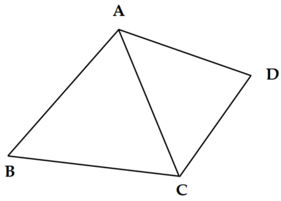
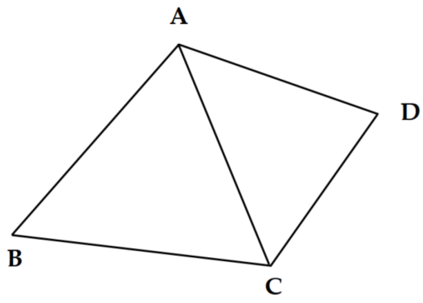
Four neighboring points, A, B, C, and D, on the reconstructed rut surface define one grid cell. Because the four points may not be located in the same plane, the grid cell was treated as a triangulated surface element rather than as a planar quadrilateral. Each grid cell was consistently divided along the diagonal AC into two triangles, ΔABC and ΔACD. Therefore, the surface area of the grid cell was determined as the sum of the areas of these two triangles.

The spatial distances AB, BC, CD, DA, and AC were calculated from the three-dimensional coordinates of the corresponding points using the Euclidean distance formula. The side lengths of ΔABC were AB, BC, and AC, whereas those of ΔACD were AC, CD, and DA.

The area of each triangle was calculated using Heron’s formula.

$$A=\sqrt{l(l-a)(l-b)(l-c)}$$

(6)

The semiperimeter used in Heron’s formula was calculated as follows:

$$l=(a+b+c)/2$$

(7)

where A is the area of an individual triangle; (a), (b), and (c) are the three side lengths of the corresponding triangle; and ($l$) is its semiperimeter. Equation (6) was applied separately to ΔABC and ΔACD to obtain A_ABC and A_ACD, respectively.

The triangulated surface area of one grid cell was then calculated as follows:

$$A_{\mathrm{A}\mathrm{B}\mathrm{C}\mathrm{D}}=A_{\mathrm{A}\mathrm{B}\mathrm{C}}+A_{\mathrm{A}\mathrm{C}\mathrm{D}}$$

(8)

where A_ABCD is the triangulated surface area of the grid cell, A_ABC is the area of ΔABC, and A_ACD is the area of ΔACD. The same diagonal direction, AC, was used for all grid cells to ensure consistency in the surface triangulation. Finally, the reconstructed three-dimensional rut-surface area was obtained by summing the triangulated surface areas of all grid cells within the analyzed region.

3. Results and Discussion

3.1. Soil Characteristic Parameters

Soil Cohesion and Soil Internal Friction Angle

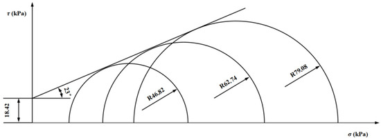
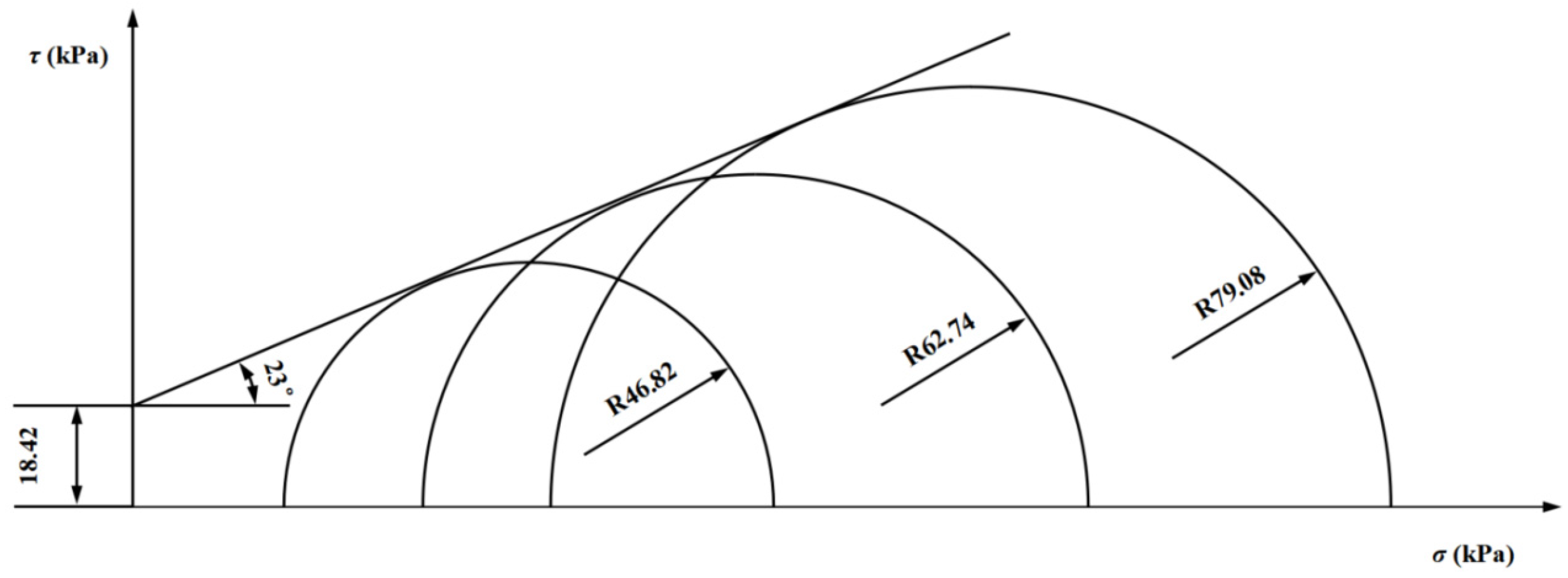
Table 2 shows the values of $({\sigma }_1+{\sigma }_3)/2$, $({\sigma }_1-{\sigma }_3)/2$, and the axial distance under different ambient pressures of four samples. Under each ambient pressure, a circle was drawn (Figure 11); the distance between 0 and the average value of $({\sigma }_1+{\sigma }_3)/2$ was taken as the center of the Mohr’s circle, and the value of $({\sigma }_1-{\sigma }_3)/2$ was taken as the radius of the Mohr’s circle. Then, the envelope of the Mohr’s circle was drawn: the Y-intercept of the envelope was the value of the soil cohesion, c (18.42 kPa), and the intersection angle between the envelope and the X-axis was the value of the soil internal friction angle ϕ (23°).

Table 2. Values of $({\sigma }_1+{\sigma }_3)/2$, $({\sigma }_1-{\sigma }_3)/2$, and axial distance under different ambient pressures.

	(σ1 + σ3)/2 (kPa)		(σ1 − σ3)/2 (kPa)		Axial Distance (mm)
Ambient Pressure (kPa)	Mean	Std. Dev.	Mean	Std. Dev.	Mean	Std. Dev.
40	75.24	9.4	46.82	1.2	4.86	0.82
80	115.39	10.53	62.74	1.65	7.94	1.17
120	156.34	11.97	79.08	1.97	12.24	0.55

Figure 11. Soil cohesion and internal friction angle.

3.2. Soil–Tire Coupling Parameters

Under static conditions, when the tire inflation pressure was 69 kPa and the tire load was 1.5 kN, a longitudinal length of 290 mm, corresponding to approximately three times the lug pitch, was observed [32]. During the experiment, the tire was in continuous motion, so it was very difficult to measure the actual contact length. Thus, in this study, a standardized longitudinal analysis window of 290 mm was adopted for all test conditions to ensure consistent comparison of the reconstructed surface geometry, and all the stress sensors were installed within the analysis window. However, the actual contact length may vary with tire inflation pressure, vertical load, and forward speed. Therefore, the reconstructed surface area obtained within this analysis window and the corresponding Mohr–Coulomb-based traction-related index were mainly used for relative comparison among the tested conditions rather than as direct measurements of the actual tire–soil contact area or absolute tractive performance.

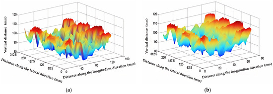
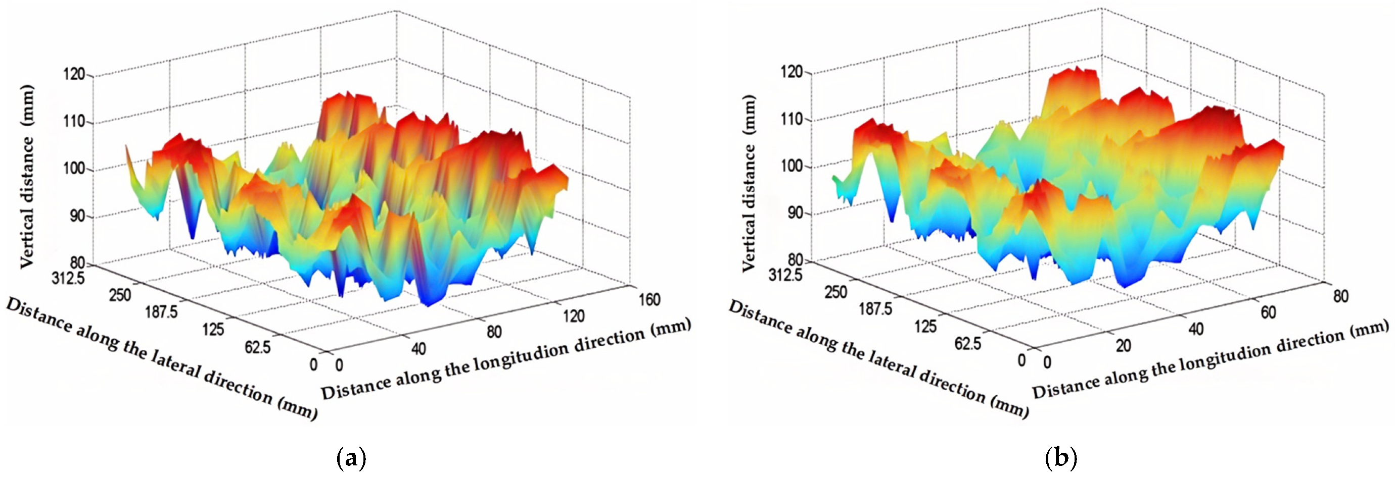
Figure 12 shows the comparison of contact area between the graphical before and after interpolation (p_i = 69 kPa, W = 1.5 kN, and S = 2 m/s). Since the laser sensor was mounted on a laser profiler (Figure 3), the vertical distance in Figure 11 was the distance between the laser sensor and the contact surface, with an initial value of 80 cm. So, the greater the soil compaction, the greater the vertical distance. Based on the iterative function system and fractal interpolation theory, the fractal dimensions of the contact surface before and after interpolation were 2.20 and 2.27, respectively, and the non-scale range was the same.

Figure 12. Comparison of the contact area in the graphics before and after interpolation (p_i = 69 kPa, W = 1.5 kN, and S = 2 m/s), and the standardized longitudinal analysis window was 290 mm. (a) Before interpolation; (b) after interpolation.

After interpolation, the fractal dimension increased slightly from 2.20 to 2.27, indicating increased local surface complexity. The similar correlation coefficients and unchanged scale-free range suggest that the overall surface characteristics were retained [32].

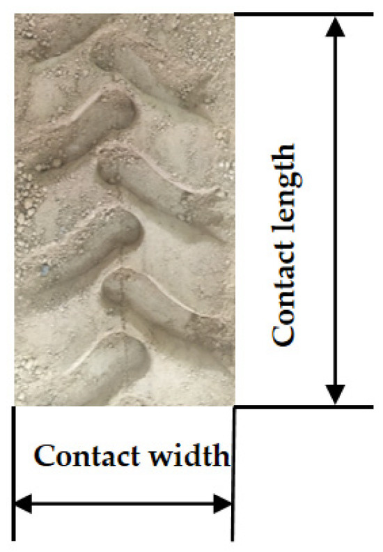
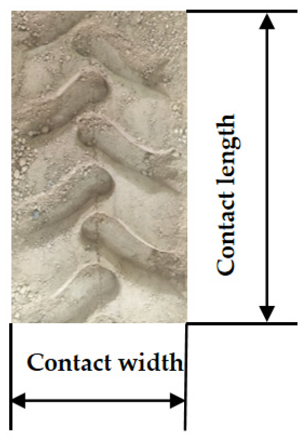
Figure 13 presents a top view of the post-pass soil rut. Alternating depressed regions and raised soil ridges can be observed within the rut and are approximately aligned with the chevron tread pattern. The depressed regions were likely generated by the passage and penetration of the tire lugs, whereas the adjacent raised regions may have resulted from the upward and lateral displacement of soil caused by tread-induced compression and shearing. The shadows visible beside the raised regions also indicate local differences in surface elevation. The apparent shadows near these apparently raised soil portions seem to support the idea that the soil is protruding upward in these places.

Figure 13. Top view of soil rut formed by a pass of the tire.

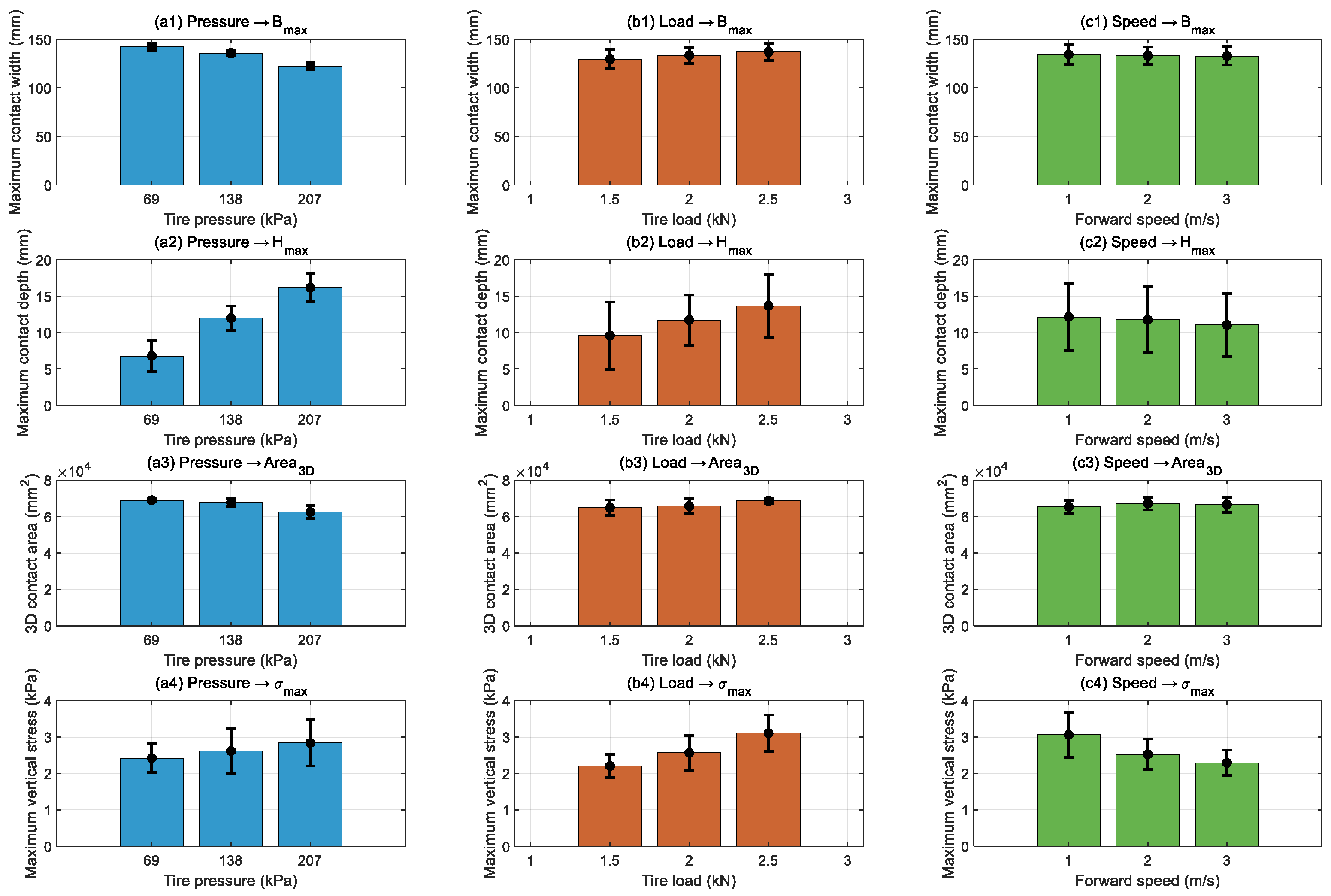
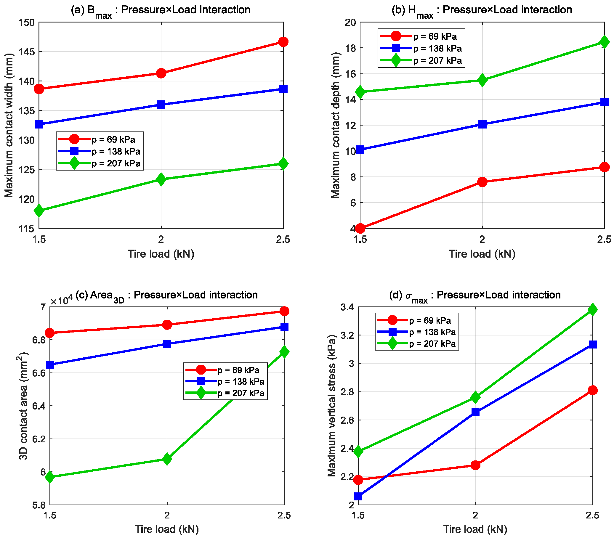
Table 3 shows the detailed measurement parameters of soil–tire coupling during the experiment. To facilitate interpretation of the factorial results, Table 3 provides the detailed values for all treatment combinations; Figure 14 illustrates the main-effect trends, Figure 15 shows the pressure–load interaction patterns, and Table 4 summarizes the corresponding ANOVA results. The following sections discuss these results, with an emphasis on the response trends and their physical interpretation.

Table 3. The detailed measurement parameters of soil–tire coupling.

Factor Levels			Experiment Results
Tire Inflation Pressure (kPa)	Tire Load (kN)	Forward Speed (m/s)	Maximum Post-Pass Rut Width (mm)	Maximum Contact Depth (mm)	2D Contact Area (mm2)	3D Contact Area (mm2)	Maximum Vertical Stress (kPa)	Sensor Number of Maximum Vertical Stress
69	1.5	1	140	4.36	40,600	67,866	2.25	11
69	1.5	2	138	4.11	40,020	68,611	2.18	11
69	1.5	3	138	3.54	40,020	68,768	2.10	11
69	2	1	144	7.95	41,760	68,192	2.39	11
69	2	2	140	7.78	40,600	69,527	2.30	11
69	2	3	140	7.10	40,600	69,015	2.15	11
69	2.5	1	148	9.21	42,920	69,527	3.38	11
69	2.5	2	146	8.99	42,340	69,730	2.68	11
69	2.5	3	146	8.08	42,340	69,934	2.37	11
138	1.5	1	134	10.82	38,860	62,908	2.27	10
138	1.5	2	132	9.96	38,280	68,089	2.08	10
138	1.5	3	132	9.56	38,280	68,491	1.83	10
138	2	1	136	12.79	39,440	66,049	3.26	10
138	2	2	136	12.03	39,440	68,451	2.51	10
138	2	3	136	11.42	39,440	68,764	2.19	10
138	2.5	1	140	14.15	40,600	67,602	3.70	10
138	2.5	2	138	13.58	40,020	69,912	3.10	10
138	2.5	3	138	13.64	40,020	68,837	2.60	10
207	1.5	1	118	15.21	34,220	59,834	2.97	10
207	1.5	2	118	14.39	34,220	60,197	2.11	10
207	1.5	3	118	14.15	34,220	59,019	2.05	10
207	2	1	124	15.23	35,960	59,840	3.45	10
207	2	2	124	15.81	35,960	62,471	2.54	10
207	2	3	122	15.46	35,380	60,026	2.29	10
207	2.5	1	128	19.67	37,120	66,833	3.87	10
207	2.5	2	126	19.19	36,540	68,458	3.24	10
207	2.5	3	126	16.56	36,540	66,524	3.03	10

Note: Each combination was processed three times by reinstalling the sensors each time (i.e., three independent replicates).

Figure 14. Main effects of inflation pressure, tire load, and forward speed on soil–tire interaction parameters.

Figure 15. Interaction effects of inflation pressure and tire load on soil–tire interaction parameters. (a) Maximum post-pass rut width; (b) Maximum contact depth; (c) 3D contact area; (d) Maximum vertical stress.

Table 4. Three-way analysis of variance (ANOVA) for soil–tire interaction parameters.

Response Variable	Source	SumSq	df	MeanSq	F-Value	p-Value	Significance
B_max	Tire pressure	1831.41	2	915.70	1545.25	<0.001	***
	Tire load	242.07	2	121.04	204.25	<0.001	***
	Forward speed	12.74	2	6.37	10.75	0.0054	**
	Pressure×Load	11.26	4	2.82	4.75	0.0294	*
	Pressure × Speed	5.93	4	1.48	2.50	0.1257	n.s.
	Load × Speed	0.59	4	0.15	0.25	0.9018	n.s.
	Error	4.74	8	0.59
H_max	Tire pressure	398.69	2	199.34	559.62	<0.001	***
	Tire load	76.00	2	38.00	106.68	<0.001	***
	Forward speed	5.57	2	2.78	7.81	0.0131	*
	Pressure × Load	6.08	4	1.52	4.26	0.0387	*
	Pressure × Speed	0.53	4	0.13	0.37	0.8216	n.s.
	Load × Speed	0.89	4	0.22	0.62	0.6581	n.s.
	Error	2.85	8	0.36
Area_3D	Tire pressure	2.08 × 108	2	1.04	153.35	<0.001	***
	Tire load	6.77 × 107	2	3.38	49.90	<0.001	***
	Forward speed	1.61 × 107	2	8.04	11.86	0.0040	**
	Pressure × Load	4.38 × 107	4	1.10	16.16	<0.001	***
	Pressure × Speed	1.19 × 107	4	2.98	4.39	0.0360	*
	Load × Speed	1.73 × 106	4	4.34	0.64	0.6490	n.s.
	Error	5.42 × 106	8	6.78
σ_max	Tire pressure	0.78	2	0.39	11.96	0.0039	**
	Tire load	3.72	2	1.86	56.89	<0.001	***
	Forward speed	2.80	2	1.40	42.79	<0.001	***
	Pressure × Load	0.24	4	0.06	1.85	0.2119	n.s.
	Pressure × Speed	0.30	4	0.07	2.27	0.1502	n.s.
	Load × Speed	0.18	4	0.05	1.39	0.3202	n.s.
	Error	0.26	8	0.03

Note: *** p < 0.001, ** p < 0.01, * p < 0.05, n.s. = not significant (p ≥ 0.05). The three-way interaction (8 degrees of freedom) was pooled as the residual error.

3.2.1. Combination Influence of Influence Factors on the Maximum Post-Pass Rut Width

The main effects of each factor on the maximum post-pass rut width are shown in Figure 14(a1–c1). It can be observed that tire inflation pressure exerts the most significant influence. When the inflation pressure increased from 69 kPa to 207 kPa, the mean post-pass rut width decreased from 142.2 mm to 122.4 mm, representing a reduction of 13.9%. As the tire load increased from 1.5 kN to 2.5 kN, the post-pass rut width increased from 129.8 mm to 137.1 mm, with an increase of 5.6%. The effect of forward speed was relatively weak, with the post-pass rut width decreasing slightly from 134.4 mm to 132.9 mm as the speed increased from 1 m/s to 3 m/s, representing a reduction of only 1.1%.

The ANOVA results in Table 4 indicate that the main effect of tire inflation pressure is highly significant (p < 0.001), the main effect of tire load is highly significant (p < 0.001), and the main effect of forward speed is very significant (p = 0.0054). Among the second-order interactions, only the interaction between inflation pressure and tire load is significant (p = 0.0294), while the interactions of inflation pressure with speed (p = 0.1257) and tire load with speed (p = 0.9018) are not significant. As shown in Figure 15a, under low inflation pressure (69 kPa), the post-pass rut width increased from 138.7 mm to 146.7 mm (an increase of 5.8%) when the tire load increased from 1.5 kN to 2.5 kN. Under high inflation pressure (207 kPa), the same load increment resulted in an increase in post-pass rut width from 118.0 mm to 126.0 mm (an increase of 6.8%). Although the relative increases were similar, the absolute increment under low inflation pressure was larger, indicating that low inflation pressure amplifies the positive effect of tire load on post-pass rut width. This trend may be attributed to the lower radial stiffness of the tire under soft tire conditions, where load increases are more readily converted into radial deformation and rut-surface expansion. area. Alkhalifa et al. [10] also reported that inflation pressure and vertical load significantly affect tire–soil contact characteristics, which verifies our statement. The maximum post-pass rut width occurred at p_i = 69 kPa, W = 2.5 kN, and S = 1 m/s (148 mm), while the minimum post-pass rut width occurred at p_i = 207 kPa, W = 1.5 kN, and S = 1 m/s (118 mm). The former results from the synergistic effect of low inflation pressure and high tire load, which allows for sufficient tire deformation, whereas the latter is due to the combined constraints of high inflation pressure and low tire load, which minimize the contact area.

3.2.2. Combination Influence of Influence Factors on the Maximum Post-Pass Rut Depth

The main effects of each factor on the maximum contact depth are shown in Figure 14(a2–c2). It can be observed that tire inflation pressure exerts the most prominent influence. When the inflation pressure increased from 69 kPa to 207 kPa, the mean contact depth increased from 6.79 mm to 16.19 mm, representing an increase of 138%. As the tire load increased from 1.5 kN to 2.5 kN, the contact depth increased from 9.57 mm to 13.67 mm, with an increase of 42.9%. As the forward speed increased from 1 m/s to 3 m/s, the contact depth slightly decreased from 12.15 mm to 11.06 mm, representing a reduction of 9.0%.

The ANOVA results in Table 4 indicate that the main effect of tire inflation pressure is highly significant (p < 0.001), the main effect of tire load is highly significant (p < 0.001), and the main effect of forward speed is significant (p = 0.0131). Among the second-order interactions, only the interaction between inflation pressure and tire load is significant (p = 0.0387), while the interactions of inflation pressure with speed (p = 0.8216) and tire load with speed (p = 0.6581) are not significant. As shown in Figure 15b, under low inflation pressure (69 kPa), the contact depth increased from 4.00 mm to 8.76 mm (an increase of 119%) when the tire load increased from 1.5 kN to 2.5 kN. Under high inflation pressure (207 kPa), the same load increment resulted in an increase in contact depth from 14.58 mm to 18.47 mm (an increase of only 26.7%), indicating that the amplifying effect of tire load on contact depth is extremely significant under low inflation pressure. This is mainly attributed to the larger contact area between the tire and soil under low inflation pressure, where load increases directly, leading to greater vertical settlement [19]. The maximum contact depth occurred at p_i = 207 kPa, W = 2.5 kN, and S = 1 m/s (19.67 mm), where the stress concentration caused by high inflation pressure synergizes with the sinking force of high tire load. The minimum contact depth occurred at p_i = 69 kPa, W = 1.5 kN, and S = 3 m/s (3.54 mm).

3.2.3. Combination Influence of Influence Factors on the Maximum 3D Post-Pass Rut-Surface Area

The main effects of each factor on the 3D post-pass rut-surface area are shown in Figure 14(a3–c3). Compared with the 2D projection area, the 3D area provides a more detailed description of the post-pass rut-surface geometry. Tire inflation pressure exerts the greatest influence. When the inflation pressure increased from 69 kPa to 207 kPa, the mean 3D post-pass rut-surface area decreased from 69,019 mm² to 62,578 mm², representing a reduction of 9.3%. As the tire load increased from 1.5 kN to 2.5 kN, the area increased from 64,865 mm² to 68,595 mm², with an increase of 5.8%. As the forward speed increased from 1 m/s to 3 m/s, the area increased from 65,406 mm² to 66,598 mm², with an increase of 1.8%.

The ANOVA results in Table 4 indicate that the main effect of tire inflation pressure is highly significant (p < 0.001), the main effect of tire load is highly significant (p < 0.001), and the main effect of forward speed is very significant (p = 0.0040). Among the second-order interactions, the interaction between inflation pressure and tire load is highly significant (p < 0.001), the interaction between inflation pressure and speed is significant (p = 0.0360), and the interaction between tire load and speed is not significant (p = 0.6490). As shown in Figure 15c, under high inflation pressure (207 kPa), the 3D post-pass rut-surface area increased from 59,683 mm² to 67,272 mm² when the tire load increased from 1.5 kN to 2.5 kN. Under low inflation pressure (69 kPa), the same load increment resulted in an increase in area from 68,415 mm² to 69,730 mm². This indicates that the post-pass rut-surface area is more sensitive to tire load under high inflation pressure, because the initial post-pass rut-surface area is smaller under high inflation pressure, and the relative proportion of post-pass rut-surface area expansion is greater when load increases. Although the interaction between inflation pressure and speed is significant (p = 0.0360), its effect size is much smaller than that of the inflation pressure–load interaction, indicating that speed primarily plays an independent moderating role rather than fundamentally altering the direction of inflation pressure effects. The maximum 3D post-pass rut-surface area occurred at p_i = 69 kPa, W = 2.5 kN, and S = 3 m/s (69,934 mm²), while the minimum 3D post-pass rut-surface area occurred at p_i = 207 kPa, W = 1.5 kN, and S = 3 m/s (59,019 mm²).

3.2.4. Combined Influence of Influencing Factors on the Maximum Vertical Stress at Each Sensor

The main effects of each factor on the maximum vertical stress are shown in Figure 14(a4–c4). Tire load exerts the greatest influence. When the tire load increased from 1.5 kN to 2.5 kN, the mean vertical stress increased from 2.20 kPa to 3.11 kPa, representing an increase of 41.4%. As the forward speed increased from 1 m/s to 3 m/s, the stress decreased from 3.06 kPa to 2.29 kPa, representing a reduction of 25.2%. As the tire inflation pressure increased from 69 kPa to 207 kPa, the stress increased from 2.42 kPa to 2.84 kPa, with an increase of 17.4%.

A recent field-scale study by Kukharets et al. [34] also demonstrated a pronounced effect of tire inflation pressure on tire–soil responses. When tire inflation pressure increased from 0.08 to 0.24 MPa, the mean calculated contact area decreased from approximately 0.397 to 0.259 m², while the corresponding surface contact stress increased from approximately 147.5 to 227.0 kPa, representing an increase of about 53.9%. In this study, increasing inflation pressure from 69 to 207 kPa increased the mean vertical stress from 2.42 to 2.84 kPa (17.4%) and decreased the mean 3D post-pass rut-surface area from 69,019 to 62,578 mm² (9.3%). Although the absolute values are not directly comparable because of differences in tire dimensions, wheel loads, soil conditions, and measurement methods, both studies indicate that tire inflation pressure has a substantial influence on tire–soil mechanical responses.

The ANOVA results in Table 4 indicate that the main effect of tire load is highly significant (p < 0.001), the main effect of forward speed is highly significant (p < 0.001), and the main effect of tire inflation pressure is very significant (p = 0.0039). Notably, none of the second-order interactions are significant, indicating that the effects of the three factors on vertical stress can be approximately treated as independent and additive. The maximum vertical stress occurred at p_i = 207 kPa, W = 2.5 kN, and S = 1 m/s (3.87 kPa, Sensor No. 10), where the combination of high inflation pressure and high tire load led to severe stress concentration. The minimum vertical stress occurred at p_i = 138 kPa, W = 1.5 kN, and S = 3 m/s (1.83 kPa, Sensor No. 10), where the combination of moderate inflation pressure, low tire load, and high forward speed achieved the greatest stress dispersion. While Yao et al. [18] focused on validating an FEM–DEM model against soil-bin measurements of drawbar pull, sinkage, and vertical stress, confirming these parameters as reliable indicators of tire–soil interaction, this study experimentally revealed the relative and interaction effects of inflation pressure, wheel load, and forward speed on tire–soil responses.

3.3. Combined Influence of Influencing Factors on the Mohr–Coulomb-Based Traction-Related Index Coefficient

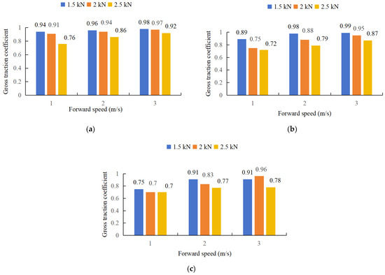
The Mohr–Coulomb-based traction-related index coefficient is a theoretical comparative parameter derived from soil shear-strength properties, vertical load, and the geometric proxy area. A higher value represents a higher calculated index within the adopted framework and should not be interpreted as a direct measurement of actual tire traction. Figure 16 illustrates the variation of the Mohr–Coulomb-based traction-related index coefficient under different combinations of tire inflation pressure, tire load, and forward speed.

Figure 16. Influence of forward speed, tire inflation pressure, and tire load on Mohr–Coulomb-based traction-related index coefficient. (a) p_i = 69 kPa; (b) p_i = 138 kPa; (c) p_i = 207 kPa.

As shown in Figure 16a, under low inflation pressure (69 kPa), the Mohr–Coulomb-based traction-related index coefficient is generally high and increases continuously with increasing forward speed. Taking the tire load of 1.5 kN as an example, the Mohr–Coulomb-based traction-related index coefficient increased from 0.94 to 0.98 as the forward speed increased from 1 m/s to 3 m/s; under the 2.5 kN load, it increased from 0.76 to 0.92. This indicates that, under low inflation pressure conditions, higher forward speed was associated with a higher calculated Mohr–Coulomb-based traction-related coefficient, which can be attributed to the slight increase in tire–soil contact area with increasing speed, reducing the vertical load per unit area and consequently improving the traction coefficient. In addition, at the same forward speed, the Mohr–Coulomb-based traction-related index coefficient decreases with increasing tire load. This trend may be associated with greater soil deformation under higher vertical loads.

Under moderate inflation pressure (138 kPa, Figure 16b), the variation of the Mohr–Coulomb-based traction-related index coefficient is more complex. At low load (1.5 kN), the Mohr–Coulomb-based traction-related index coefficient increased from 0.89 to 0.99 with increasing forward speed, reaching the maximum value of 0.99 among all test conditions at 3 m/s. At moderate load (2 kN), the Mohr–Coulomb-based traction-related index coefficient increased from 0.75 to 0.95. At high load (2.5 kN), although the Mohr–Coulomb-based traction-related index coefficient also increased from 0.72 to 0.87 with increasing forward speed, the overall values remained relatively low. This indicates that, under moderate inflation pressure, the effect of forward speed on the calculated traction-related coefficient decreased with increasing tire load.

Under high inflation pressure (207 kPa, Figure 16c), the Mohr–Coulomb-based traction-related index coefficient also exhibits an increasing trend with forward speed: from 0.75 to 0.91 at low load (1.5 kN), from 0.70 to 0.96 at moderate load (2 kN), and from 0.70 to 0.78 at high load (2.5 kN). However, the increase at high load (11.4%) is much smaller than that at low load (21.3%) and moderate load (37.1%), and its maximum value of 0.78 is significantly lower than the 0.91 and 0.96 observed under low and moderate load conditions. This indicates that high inflation pressure results in an excessively small tire contact area, which, when combined with high load, causes a sharp increase in vertical load per unit area and excessive soil shear failure. Consequently, the increase in the calculated traction-related coefficient with forward speed became less pronounced under the high-load condition.

The average traction force of the orthogonal test (a total of nine experiments in different forward speed, tire load, and inflation pressures) of the tire predicted from Figure 16 was 1.71 kN, which was a little more than the actual traction force, and the error value was 0.04 kN, meaning that the proposed index was meaningfully related to the measured traction value.

Overall, the calculated traction-related coefficient tended to decrease with increasing tire inflation pressure, although slight non-monotonic variations occurred under some test conditions. For example, at 1.5 kN and 3 m/s, the Mohr–Coulomb-based traction-related index coefficient was 0.98 at 69 kPa, 0.99 at 138 kPa, decreasing to 0.91 at 207 kPa. At 2.5 kN and 1 m/s, it was 0.76 at 69 kPa, 0.72 at 138 kPa, and 0.70 at 207 kPa. This demonstrates that low inflation pressure effectively improves the Mohr–Coulomb-based traction-related index coefficient by increasing the contact area and reducing the vertical load per unit area. Martelli et al. [26] found that increasing front ballast reduced tire slip and slightly improved tractor traction efficiency. In contrast, this study showed that increasing single-wheel vertical load generally reduced the traction-related coefficient, indicating different load effects at the vehicle and tire–soil interface levels.

The present results can also be viewed in the broader context of soil–machine interaction, in which the geometry and operating conditions of soil-engaging components affect soil resistance, energy consumption, soil transport, and mechanical loading during tillage [35,36]. In addition, Swamy et al. [37] systematically reviewed tire–deformable soil interaction studies and identified velocity, inflation pressure, and normal load as important sensitivity parameters in tire–soil modeling and evaluation. This study further examined the main and interaction effects of these operating factors under controlled single-wheel soil-bin conditions, thereby providing experimental evidence that complements the broader findings summarized in the review.

4. Conclusions

In this study, we integrated laser 3D reconstruction of tire–soil contact geometry, in-situ soil stress measurement, and traction-force acquisition to analyze the joint effects of inflation pressure, vertical load, and forward speed on the gross traction coefficient. Under the same driving-wheel test setup, qualitative characterizations of contact-geometry evolution, soil–stress distribution, and traction performance were performed simultaneously to predict the gross traction coefficient for evaluating vehicle trafficability. Although this method has certain limitations because we ignored the slip ratio and tread-relevant factors, which limits the conclusions, it still has practical research significance. We reached the following conclusions:

(1) Tire inflation pressure exerts the most significant influence on tractive performance, followed by tire load, while forward speed shows a relatively minor effect. The interaction between inflation pressure and load significantly affects soil–tire coupling parameters, whereas interactions involving speed are not significant. The combination of low tire load, low inflation pressure, and high forward speed (W = 1.5 kN, p_i = 138 kPa, S = 3 m/s) yielded the maximum Mohr–Coulomb-based traction-related index coefficient (0.99) among all tested conditions, representing the optimal tractive performance under the experiment conditions in this study.

(2) The Mohr–Coulomb-based traction-related index coefficient increases with increasing forward speed but decreases with increasing tire load. Under the tested conditions, low inflation pressure was associated with a higher Mohr–Coulomb-based traction-related index coefficient, partly due to the larger geometric proxy area and lower vertical load per unit area.

(3) Under the tested single-wheel soil-bin conditions, lower inflation pressure and appropriate adjustment of forward speed were associated with relatively higher calculated traction-related indices. These results may provide a reference for tire inflation pressure and operating-speed management, while further field validation is required before broader practical application.

5. Limitations and Future Research

(1) The experiments were conducted using a single tire on a soil bin. Although the tire was a general-purpose tire and the soil parameters were chosen to simulate those of field soil, the results of the experiments were still different from the actual field conditions.

(2) The tractive performance of the tractor was governed by soil and tire parameters, soil–tire coupling, the structure and operation parameters, and so on; it was a comprehensive model. In this paper, the Mohr–Coulomb-based traction-related index coefficient was calculated based on the factors that influenced soil cohesion and the soil internal friction angle, dynamic load, and contact area between the soil and tire, and ignored other, related influencing factors. In addition, a standardized longitudinal analysis window of 290 mm was adopted rather than the actual dynamic tire–soil contact length.

(3) For future work, additional influencing factors, different soil conditions, different tractors or tires, and different experiment fields should be considered to perfect the prediction model. Therefore, further validation using measured traction data and field experiments is required before these results can be extended to broader practical applications.

(4) This method has certain limitations since we ignored the slip ratio and tread-relevant factors, which limits the conclusions. Furthermore, some new technologies, such as digital twin technology, should be taken into account.

References

- Kim, W.S.; Baek, S.Y.; Kim, T.J.; Kim, Y.S.; Park, S.U.; Choi, C.H.; Hong, S.J.; Kim, Y.J. Workload analysis for determination of the reduction gear ratio for a 78 kW all-wheel drive electric tractor design. Korean J. Agric. Sci. 2019, 46, 613–627. [Google Scholar] [CrossRef] [Scilit]
- Kim, W.S.; Kim, Y.S.; Kim, T.J.; Park, S.U.; Choi, Y.; Choi, S.R.; Kim, Y.K.; Kim, Y.J. Analysis of power requirement of 78 kW class agricultural tractor according to the major field operation. Trans. Korean Soc. Mech. Eng. A. 2019, 43, 911–922. [Google Scholar] [CrossRef] [Scilit]
- Grisso, R.; Perumpral, J.; Zoz, F. An empirical model for tractive performance of rubber-tracks in agricultural soils. J. Terramech. 2006, 43, 225–236. [Google Scholar] [CrossRef] [Scilit]
- Kim, W.S.; Kim, Y.J.; Park, S.U.; Kim, Y.S. Influence of soil moisture content on the traction performance of a 78-kW agricultural tractor during plow tillage. Soil Tillage Res. 2021, 207, 104851. [Google Scholar] [CrossRef] [Scilit]
- Baek, S.M.; Kim, W.S.; Kim, Y.S.; Lee, N.G.; Kim, N.H.; Kim, Y.J. Analysis of the load distribution and contact safety factor of PTO gears of a 71 kW class agricultural tractor. Korean J. Agric. Sci. 2020, 47, 327–335. [Google Scholar] [CrossRef] [Scilit]
- Ebrahimi, E.; Tekeste, M.Z.; Huth, N.I.; Antille, D.L.; Archontoulis, S.V.; Horton, R. Measured and modeled maize and soybean growth and water use on pipeline disturbed land. Soil Tillage Res. 2022, 220, 105–340. [Google Scholar] [CrossRef] [Scilit]
- Tekeste, M.Z.; Way, T.R.; Birkenholz, W.; Brodbeck, S. Effect of increased deflection tire technology on soil compaction. J. ASABE 2023, 66, 75–84. [Google Scholar] [CrossRef] [Scilit]
- Singh, C.D.; Singh, R.C. Computerized instrumentation system for monitoring the tractor performance in the field. J. Terramech. 2011, 48, 333–338. [Google Scholar] [CrossRef] [Scilit]
- Zhu, Z.; Chen, L.; Xia, C.; Cai, Y. Test research on the adhesive and tractive performance of a wheeled tractor. Int. J. Heavy Veh. Syst. 2020, 27, 65–82. Available online: https://www.inderscience.com/offers.phd?id=104425 (accessed on 1 August 2026). [CrossRef] [Scilit]
- Alkhalifa, N.; Tekeste, M.Z.; Jiagwe, P.; Way, T.R. Effects of vertical load and inflation pressure on tire-soil interaction on artificial soil. J. Terramech. 2024, 112, 19–34. [Google Scholar] [CrossRef] [Scilit]
- Way, T.R.; Kishimoto, T.; Burt, E.C.; Bailey, A.C. Tractor tire aspect ratio effects on soil stresses and rut depths. Trans. ASAE 1997, 40, 871–881. [Google Scholar] [CrossRef] [Scilit]
- Sandu, C.; Worley, M.E.; Morgan, J.P. Experimental study on the contact patch pressure and sinkage of a lightweight vehicle on sand. J. Terramech. 2010, 47, 343–359. [Google Scholar] [CrossRef] [Scilit]
- Naranjo, S.; Sandu, C.; Taheri, S.; Taheri, S. Experimental testing of an off-road instrumented tire on soft soil. J. Terramech. 2014, 56, 119–137. [Google Scholar] [CrossRef] [Scilit]
- He, R.; Sandu, C.; Osorio, J.E. Systematic tests for study of tire tractive performance on soft soil: Part II—Parameterization of terramechanics model and tire model. J. Terramech. 2019, 85, 77–88. [Google Scholar] [CrossRef] [Scilit]
- Wulfsohn, D. Soil-tire contact area. In Advances in Soil Dynamics; Upadhyaya, S.K., Chancellor, W.J., Perumpral, J.V., Gill, W.R., Way, T.R., Wulfsohn, D., Eds.; ASABE: St. Joseph, MI, USA, 2009; Volume 3. [Google Scholar]
- Wulfsohn, D. Traction device-soil interfacial behavior. In Advances in Soil Dynamics; Upadhyaya, S.K., Chancellor, W.J., Perumpral, J.V., Gill, W.R., Way, T.R., Wulfsohn, D., Eds.; ASABE: St. Joseph, MI, USA, 2009; Volume 3. [Google Scholar]
- Freitag, D.R. Soil Dynamics as related to traction and transport systems. In Proc. Intl. Conf. On Soil Dynamics.; Auburn University: Auburn, AL, USA, 1985; Volume 4, pp. 605–629. [Google Scholar]
- Yao, L.; Zhu, Y.; Wang, Y.; Shi, D.; Pang, S. Research of tire-soil interaction based on FEM-DEM for small wheeled mobile platform in forest. Adv. Eng. Softw. 2024, 196, 103735. [Google Scholar] [CrossRef] [Scilit]
- Zeng, H.; Lin, Z.; Huang, G.; Yang, X.; Li, Y.; Su, J.; Xu, W. Parameter identification of DEM-FEM coupling model to simulate traction behavior of tire-soil interaction. J. Terramech. 2025, 117, 101012. [Google Scholar] [CrossRef] [Scilit]
- Yang, P.; Zang, M.; Zeng, H. An efficient 3D DEM-FEM contact detection algorithm for tire-sand interaction. Powder Technol. 2020, 360, 1102–1116. [Google Scholar] [CrossRef] [Scilit]
- Upadhyaya, S.K. Traction prediction equations. In Advances in Soil Dynamics; Upadhyaya, S.K., Chancellor, W.J., Perumpral, J.V., Gill, W.R., Way, T.R., Wulfsohn, D., Eds.; ASABE: St. Joseph, MI, USA, 2009; Volume 3. [Google Scholar]
- Upadhyaya, S.K.; Wulfsohn, D. Traction prediction using soil parameters obtained with an instrumented analog device. J. Terramech. 1993, 30, 85–100. [Google Scholar] [CrossRef] [Scilit]
- Wong, J.Y. Computer aided analysis of the effects of design parameters on the performance of tracked vehicles. J. Terramech. 1986, 23, 95–124. [Google Scholar] [CrossRef] [Scilit]
- Moro, T. Tractive performance of a bulldozer running on weak ground. J. Terramech. 1989, 26, 249–273. [Google Scholar] [CrossRef] [Scilit]
- Venturini, S.; Bonisoli, E.; Rosso, C.; Velardocchia, M. A tyre-rim interaction digital twin for biaxial loading conditions. Mech. Mach. Theory 2024, 191, 105491. [Google Scholar] [CrossRef] [Scilit]
- Martelli, M.; Chiarabelli, D.; Gessi, S.; Marani, P.; Mucchi, E.; Polastri, M. Comprehensive lumped parameter and multibody approach for the dynamic simulation of agricultural tractors with tyre–soil interaction. IET Cyber-Syst. Robot. 2023, 5, e12092. [Google Scholar] [CrossRef] [Scilit]
- Guo, D.; Wang, L.; Du, Y.; Wu, Z.; Zhang, W.; Zhi, Q.; Ma, R. Online optimization of adjustable settings for agricultural machinery assisted by digital twin. Comput. Electron. Agric. 2024, 227, 109504. [Google Scholar] [CrossRef] [Scilit]
- Jiang, C.; Lu, Z.; Dong, W.; Cao, B.; Shin, K. Measurement and Analysis of the Influence Factors of Tractor Tire Contact Area Based on a Multiple Linear Regression Equation. Sustainability 2023, 15, 10017. [Google Scholar] [CrossRef] [Scilit]
- GB/T 50123-2019; Standard for Geotechnical Testing Method. Standards Press of China: Beijing, China, 2019. Available online: https://www.mohurd.gov.cn/gongkai/zc/wjk/art/2019/art_17339_241309.html (accessed on 1 August 2026).
- Zhuang, J. Calculating the Ground Mechanics of Agricultural Vehicles; China Machine Press: Beijing, China, 2002. [Google Scholar]
- Islam, M.N.; Iqbal, M.Z.; Kabir, M.S.; Jung, K.Y.; Mun, D.H.; Chung, S.O. Performance evaluation of trenchless subsurface drainage piping machine. J. Biosyst. Eng. 2019, 1, 1–8. [Google Scholar] [CrossRef] [Scilit]
- Jiang, C.; Lu, Z.; Upadhyaya, S.K.; Chen, F. Vertical stress distribution rules in compacted topsoil under tire with chevron tread pattern. Trans. Chin. Soc. Agric. Eng. 2019, 35, 80–87, (In Chinese with English abstract). [Google Scholar] [CrossRef]
- Barnsley, M.F. Fractal functions and interpolation. Constr. Approx. 1986, 2, 303–329. [Google Scholar] [CrossRef] [Scilit]
- Kukharets, S.; Zabrodskyi, A.; Sheludchenko, B.; Jasinskas, A.; Domeika, R.; Šarauskis, E. Assessment of changes in soil contact stress depending on tractor tire parameters. Sci. Rep. 2025, 15, 172. [Google Scholar] [CrossRef] [Scilit] [PubMed]
- Syromyatnikov, Y.N.; Mozgovsky, A.F.; Kalimullin, M.N.; Tikhonov, E.A.; Dzjasheev, A.-M.S.; Orekhovskaya, A.A.; Taraban, M.V. Substantiation of flat blade parameters for soil loosening. IOP Conf. Ser. Earth Environ. Sci. 2022, 981, 042043. [Google Scholar] [CrossRef] [Scilit]
- Syromyatnikov, Y.; Kuts, A.; Troyanovskaya, I.; Orekhovskaya, A.; Tikhonov, E.; Sokolova, V. Transporting ability calculation of the rotor of soil-cultivating loosening and separating vehicle. Acta Technol. Agric. 2022, 25, 73–78. [Google Scholar] [CrossRef] [Scilit]
- Swamy, V.S.; Pandit, R.; Yerro, A.; Sandu, C.; Rizzo, D.M.; Sebeck, K.; Gorsich, D. Review of modeling and validation techniques for tire-deformable soil interactions. J. Terramech. 2023, 109, 73–92. [Google Scholar] [CrossRef] [Scilit]
Disclaimer/Publisher’s Note: The statements, opinions and data contained in all publications are solely those of the individual author(s) and contributor(s) and not of MDPI and/or the editor(s). MDPI and/or the editor(s) disclaim responsibility for any injury to people or property resulting from any ideas, methods, instructions or products referred to in the content. |
© 2026 by the authors. Licensee MDPI, Basel, Switzerland. This article is an open access article distributed under the terms and conditions of the Creative Commons Attribution (CC BY) license.