


Abstract
The widespread adoption of unmanned agricultural machinery has transformed modern agricultural production. In unstructured farmland scenarios, variations in soil conditions and operational loads induce large perturbations to system dynamic parameters, leading to degraded tracking accuracy and insufficient robustness in fixed-parameter path tracking controllers. Additionally, conventional single-structure observers cannot simultaneously achieve fast convergence and smooth steady-state output. This study constructs a mixed preview error state-space equation, which aggregates parameter perturbations, unmodeled dynamics, and external disturbances into a unified lumped disturbance term of the system. A composite observer architecture is designed by parallelly combining an adaptive generalized super-twisting observer and a nonlinear extended state observer, where observation weights are continuously and smoothly scheduled via online identification of field operation conditions. Furthermore, a gain-power dual-adaptive super-twisting sliding mode control strategy is proposed, and the closed-loop stability of the system is rigorously proven. Co-simulation and field experiments covering powered rotary tillage, high-speed unloaded transfer, and variable tire pressure conditions verify that, under parameter perturbation, the increase in tracking error remains within 10%. Compared with the conventional PID controller used as a benchmark, the proposed controller reduces the root mean square error (RMSE) of lateral deviation by 40–50%, and maintains centimeter-level tracking accuracy in field operations. The proposed method provides technical support for high-precision operation of agricultural machinery in unstructured farmland environments.
1. Introduction
The popularization of unmanned agricultural machinery has effectively addressed long-standing industry challenges including low operational precision, high labor costs, intense physical workload, and limited operating hours. It enables centimeter-level precision in tillage, sowing, management, and harvesting, driving the transition from labor-intensive to technology-intensive agricultural production and reshaping modern agricultural production models [1,2]. At present, unmanned agricultural machinery covers the full spectrum of mechanized field operations [3]. The automatic navigation control system follows a core chain of positioning—perception—control—execution, supporting high-precision autonomous operation [4]. Path tracking is the core functional module, directly determining row alignment accuracy, operational coverage, and operational stability. It receives reference trajectories from global path planning and regulates steering and driving parameters in real time to maintain lateral and heading deviations within agronomic tolerances, ensuring consistency and standardization across seeding, fertilizing, and harvesting [5,6,7]. The agricultural machinery dynamic model serves as the research foundation for path tracking control. In field operations, machinery is affected by multi-source disturbances including soil adhesion, terrain slope, and operational loads, exhibiting strongly nonlinear and time-varying behavior [8,9]. An accurate dynamic model fully describes the force-motion coupling during steering, driving, and field operations, providing reliable state prediction and error feedback for control algorithm design.
During field operations, multiple dynamic parameters exhibit significant perturbation characteristics [10]. Total vehicle mass and yaw moment of inertia vary in real time with mounted implements, material consumption, and chassis mud accumulation, while the center of mass shifts concurrently, altering system inertia properties and axle load distribution [11]. Tire cornering stiffness is jointly affected by soil type, moisture content, mud depth, and vertical load, with fluctuations exceeding 30% across different fields and operational stages [12,13]. The equivalent soil adhesion coefficient and rolling resistance coefficient vary continuously with soil compaction and surface conditions, determining the saturation boundary of tire force output. These parameter perturbations cause mismatch between the nominal model and the actual system, degrading tracking accuracy and weakening robustness of fixed-parameter controllers [14,15]. In severe cases, system oscillation and sideslip occur, constraining automatic navigation performance and reliability. Parameter perturbations are coupled with unmodeled wheel–soil interaction dynamics and random field travel disturbances, which can be uniformly treated as system lumped disturbance.
Sliding mode control possesses inherent robustness against matched disturbances, features fast response, and requires no online system parameter identification, making it a mainstream approach for disturbance rejection in agricultural machinery path tracking [16,17]. Existing observers and sliding mode controllers nevertheless exhibit performance limitations. A single-structure observer cannot simultaneously achieve fast convergence and smooth steady-state output [18]. Conventional two-stage estimation architectures suffer from error propagation and accumulation. Disturbance observers face an inherent trade-off between convergence speed and noise attenuation, lack physical boundary constraints for parameter perturbations, and exhibit insufficient estimation reliability under extreme conditions [19,20]. Most sliding mode controllers adopt fixed-gain designs tuned for worst-case conditions, resulting in redundant steady-state gain and pronounced chattering [21]. A single reaching law cannot accommodate full-operating-condition requirements. Most schemes achieve only single-dimensional adaptation of the disturbance upper bound, providing insufficient rejection of unmatched parameter perturbations, with noticeable tracking accuracy degradation under large parameter variations [22,23,24,25].
Numerous scholars have conducted extensive research on path tracking of unmanned agricultural machinery. Liu et al. proposed an adaptive sliding mode predictive control algorithm combining model predictive control and sliding mode control, with online adjustment of the prediction horizon through fuzzy rules, improving tracking accuracy and dynamic performance of wheeled agricultural machinery [26]. Zhang et al. developed an ROS-based navigation system for orchard wheeled mowers, employing an adaptive pure pursuit algorithm for inter-row path tracking and verifying closed-loop feasibility through field experiments [27]. Bin Salamah et al. designed a sliding mode controller for tractor-trailer reversing with an anti-jackknifing protection mechanism, validating tracking stability through multiple simulation cases [28]. Zeng et al. proposed a super-twisting sliding mode control method based on crested porcupine optimization, constructing a multi-criteria parameter optimization framework that improved the tracking accuracy and steering smoothness of differential-drive tracked agricultural machinery [29]. Ren et al. proposed a Double-DQN-based navigation control algorithm for trailed sprayers, representing pose relationships through a virtual radar model and enhancing tracking performance on complex orchard paths [30]. Zhu et al. combined prescribed performance control with sliding mode control, strictly constraining tracking error bounds and strengthening tractor resistance to parameter perturbations and external disturbances [31]. Wang et al. proposed an improved Stanley and sliding mode composite control scheme considering sideslip compensation, effectively reducing the impact of field sideslip on tractor tracking accuracy [32]. Existing studies predominantly employ single observation structures or fixed-gain control strategies, with insufficient consideration of the coupled effects of model parameter perturbations and field lumped disturbances. Simultaneous achievement of fast error convergence and steady-state tracking accuracy under unstructured field conditions remains challenging, leaving room for improvement in controller robustness.
To address the aforementioned issues, this study proposes a dual-adaptive multi-power super-twisting sliding mode (DAMSTSM) path tracking control method based on a composite observer, to satisfy high-precision tracking requirements under large-scale field parameter perturbations. First, a dynamic model for agricultural machinery that considers tire cornering characteristics is established, and a mixed preview error state-space equation is constructed, which incorporates parameter perturbations, unmodeled dynamics, and external disturbances into the system’s lumped disturbance. Next, an adaptive generalized super-twisting observer (AGSTO) and a nonlinear extended state observer (NESO) are fused to estimate system states and lumped disturbance. A field operation condition identification module and a continuous weight fusion mechanism are introduced to dynamically match the optimal observation strategy, enabling high-precision estimation of both system states and lumped disturbance. Based on the estimated states, a multi-power reaching law super-twisting sliding mode controller is developed with a gain-power dual-adaptive regulation mechanism. This design ensures fast convergence under large initial deviations while effectively suppressing steady-state chattering. Finally, co-simulation on CarSim-Simulink platform and field vehicle tests verify the tracking accuracy and robustness of the proposed method under parameter perturbation conditions. This work provides technical support for high-precision operations of unmanned agricultural machinery in complex field environments.
2. Materials and Methods
2.1. Construction of State-Space Equation for Agricultural Machinery Path Tracking Based on Vehicle Dynamics
The kinematic model does not account for tire–soil interaction, sideslip, or other dynamic effects, yielding insufficient accuracy under wet and soft field conditions or high-speed steering. The dynamic model, based on rigid body dynamics and tire contact mechanics, describes the dynamic coupling among vehicle pose, velocity, and forces. It can realistically represent motion response under sideslip and external disturbances, making it suitable for high-speed operation, large-curvature steering, or wet farmland conditions where tire sideslip effects are significant. This model provides an accurate controlled-plant representation for high-precision robust control algorithm design.
The agricultural machinery is simplified as a two-degree-of-freedom single-track bicycle model, as shown in Figure 1. This model consolidates the left and right wheels of each axle into one equivalent wheel and is a standard and widely adopted simplification in vehicle dynamics and agricultural machinery path tracking control, since it captures the dominant lateral and yaw dynamics under the low-speed, small-sideslip-angle conditions typical of field operations while keeping the controller design tractable. XOY denotes the global coordinate system, xoy the vehicle body coordinate system, C the center of mass, P1 and P2 points on the reference path, and P3 the preview point. denotes the lateral deviation; , , and denote the vehicle travel speed and the longitudinal and lateral velocities at the center of mass, respectively; is the wheelbase; and are the distances from the center of mass to the front and rear axles, respectively; is the equivalent front wheel steering angle; and are the front and rear tire sideslip angles, respectively; is the preview distance along the vehicle longitudinal axis; is the deviation from preview point P3 to the reference path, which integrates the current lateral deviation and heading deviation .
Figure 1.
Agricultural machinery dynamic model.
To construct the dynamic model required for path tracking control analysis, the following reasonable assumptions are made: (1) the vehicle frame is rigid, the center of mass lies in the longitudinal symmetry plane, and frame elastic deformation as well as pitch and roll motions are neglected; (2) tires operate in the linear cornering region, cornering force varies linearly with sideslip angle, tire nonlinear hysteresis and relaxation effects and tire pressure variations are neglected, and left–right cornering stiffness is symmetric for both axles.
Under field operating conditions satisfying , the path tracking error dynamics can be written as
where is the curvature of the reference path at s, and is the vehicle yaw rate.
The lateral deviation is directly affected by the sideslip angle , which cannot be directly controlled through front wheel steering. The heading deviation and lateral deviation are strongly coupled, making simultaneous convergence of both deviations difficult with conventional control methods. Given the underactuated coupling characteristics of agricultural machinery path tracking, an auxiliary preview error variable is introduced to construct a mixed preview error model.
For low-speed, small-curvature steering conditions, the lateral deviation and heading deviation are fused through first-order weighting to construct the auxiliary mixed preview error model as follows
Driving the mixed preview error to zero ensures that both the lateral deviation and heading deviation converge to zero, achieving high-quality path tracking for unmanned agricultural machinery. Taking the first derivative of the auxiliary mixed preview error variable and substituting into the error dynamics of Equation (1) yields the first-order dynamics of the auxiliary mixed preview error
Taking the second derivative of the auxiliary mixed preview error variable and combining with the two-degree-of-freedom dynamic model yields the second-order preview error dynamics. Linearizing the two-degree-of-freedom single-track model about the operating point gives the sideslip-angle and yaw rate state equations in Equation (5), whose coefficient entries , , , , and are explicitly defined in Equation (6), where m, Iz, Cf and Cr denote the vehicle mass, yaw moment of inertia and front and rear cornering stiffnesses.
where is the vehicle velocity along the tangent to the reference path, and is the system lumped disturbance term, including errors caused by tire sideslip, soil resistance, and reference path curvature variations.
Defining two new state variables as and , the state-space equation can be established as
2.2. Design of AGSTO-NESO Composite Architecture State Observer Triggered by Agricultural Machinery Condition Identification
Field operations cover initial line acquisition, headland turning, long-distance straight-line operation, and inter-block transfer. Spatial variations in soil moisture and compaction, together with implement load changes, cause periodic fluctuations in wheel–soil disturbance intensity and path tracking deviation magnitude. A single-structure state observer cannot cover full-operating-condition performance requirements. Sliding mode observers feature finite-time convergence and strong parameter perturbation rejection, but their switching characteristics amplify RTK positioning noise and tend to induce high-frequency hydraulic steering actuator motion during steady state, accelerating mechanism wear. The ESO has a simple structure and smooth output, but its convergence speed is limited under large initial deviations and strong disturbances, with tracking overshoot likely during headland line acquisition. An AGSTO-NESO parallel composite architecture with condition-triggered weight scheduling dynamically matches the optimal observation strategy based on deviation magnitude, path curvature, and disturbance intensity. Without additional hardware cost or embedded computing burden, it achieves coordinated improvement of dynamic convergence performance and steady-state output quality, providing reliable state and disturbance estimation for high-precision path tracking under coupled parameter perturbations and disturbances.
2.2.1. Model Reformulation
The established second-order mixed preview error state-space model is rewritten in the following standard form
where the state variable is the mixed preview error, directly computable from vehicle pose obtained via RTK-GNSS and reference path geometry, serving as the measurable system output; x2 is the first derivative of the preview error, not directly obtainable through conventional onboard sensors and thus an unknown state to be estimated; is the known system nonlinearity, including sideslip-angle dynamics, yaw rate coupling, and path curvature effects computable from the model; is the equivalent front wheel angle, i.e., the control input; is the control gain coefficient, determined by vehicle dynamic parameters and preview distance; is the system lumped disturbance, including tire cornering force disturbances, soil resistance fluctuations, equivalent parameter perturbation terms, and unmodeled dynamics, with strong time-varying magnitude and derivative under field conditions.
Assume the derivative of the lumped disturbance is bounded, i.e., there exists an unknown positive constant such that for all
2.2.2. Adaptive Generalized Super-Twisting Observer Design
The AGSTO belongs to the class of second-order sliding mode observers and can achieve finite-time estimation of unknown states using only the measurable output, with inherent robustness to matched-channel disturbances. To reduce the conservatism of fixed-gain design and accommodate time-varying field conditions, time-varying adaptive gains are introduced. The adaptive generalized super-twisting observer is constructed as follows
where and are the observed estimates of states and , respectively; is the observation error of the measurable state; and are time-varying adaptive observation gains; and are generalized super-twisting nonlinear functions, defined as
where is a nonlinear coefficient to be designed.
Subtracting the observer equations from the system equations and defining the state observation error , the error dynamics are derived as
To ensure observation gains adjust dynamically within a reasonable range, avoiding convergence failure from excessively small gains and noise amplification from excessively large gains, an adaptive law with projection constraints is used to regulate the gain parameters as follows
where and are adaptive learning rates governing the speed of gain adjustment; , , , and are gain bounds derived from the physical range of agricultural machinery parameter perturbations. Under large-deviation conditions, the observation error increases and gains rise automatically to ensure finite-time convergence speed. Under small-deviation steady-state conditions, gains decrease gradually to suppress measurement noise amplification and high-frequency chattering. The gain bounds ensure basic convergence capability under extreme conditions while preventing abnormal gain drift.
The AGSTO obtains the lumped disturbance estimate through the equivalent output injection method. During sliding motion, the integral output of the super-twisting switching term contains unknown disturbance information. Low-pass filtering of this signal removes high-frequency switching chattering, and the extracted continuous equivalent component is the estimate of .
2.2.3. Nonlinear Extended State Observer Design
The NESO treats the lumped disturbance as an additional state variable to achieve simultaneous estimation of system states and total disturbance, with a simple structure and smooth output. For the second-order preview error system, the lumped disturbance is expanded as a third state variable , transforming the original system into a third-order extended system expressed as
A nonlinear power function is introduced to construct the NESO. This function provides high gain for small errors and low gain for large errors, balancing convergence speed and noise rejection. The nonlinear power function is defined as
where is the nonlinear factor and is the linear-segment filtering threshold, used to avoid high-frequency oscillation caused by power operations near the origin. Based on the third-order extended system, the NESO is constructed as follows:
where and are the estimates of states and , respectively; is the estimate of the lumped disturbance ; , , and are observer gain parameters tuned via the bandwidth method, with , , , where is the observer bandwidth; and are nonlinear power coefficients, typically chosen as and to achieve hierarchical convergence characteristics.
This observer requires only the preview error and control input signals to simultaneously output state and disturbance estimates, without additional sensing information. Under steady-state operating conditions, the observation output is smooth and chattering-free, effectively reducing high-frequency actuation of the steering mechanism.
2.2.4. Field Operation Condition Identification and Weight Fusion Mechanism
Field operations can be divided into typical stages with different observer performance requirements. Physical quantities directly available from the navigation system are selected as condition identification features without additional hardware sensors. The selected features are (1) preview error magnitude , reflecting the current path tracking deviation and serving as the key indicator distinguishing large-deviation line acquisition from steady-state tracking; (2) reference path curvature , reflecting the geometric characteristics of the current path segment and distinguishing straight-line operation from large-curvature turning; (3) lumped disturbance estimate derivative , reflecting the severity of disturbance abrupt changes caused by soil conditions, loads, and implement states; (4) vehicle longitudinal speed , assisting in stage identification and distinguishing low-speed headland turning from high-speed field operation.
Based on the full-process characteristics of field operations, three typical conditions are classified, corresponding to different observer-dominant strategies.
- (1)
- Large-deviation convergence condition, corresponding to initial line acquisition, headland-turning entry, and inter-block line re-engagement. The condition is satisfied when either or . Here is the preview error threshold corresponding to the acceptable tracking accuracy limit for field operations, and is the curvature threshold distinguishing straight-line operation from large-curvature turning. Convergence speed is prioritized under this condition, with AGSTO dominating.
- (2)
- Steady-state tracking condition, corresponding to straight-line field operation and constant-speed operation on small-curvature paths. All of the following must hold simultaneously: , , and . Here is the disturbance derivative threshold corresponding to the upper limit of normal soil fluctuation. Output smoothness is prioritized under this condition, with the NESO dominating.
- (3)
- Strong disturbance abrupt-change condition, corresponding to sudden entry into soft mud, implement entry/exit, load abrupt changes, and slope operation. The condition is with the preview error magnitude increasing over two consecutive control cycles. The AGSTO weight is temporarily increased under this condition to enhance disturbance rejection.
To avoid observation output jumps and control impacts caused by hard condition switching, continuous weighted fusion is adopted for smooth transition between the two observers. A weight coefficient is defined, where gives AGSTO full dominance and gives NESO full dominance. A hyperbolic tangent function is used to construct a continuous weight function with preview error as input:
where is the transition interval width governing the smoothness of switching. When is much larger than the threshold, approaches ; when is much smaller, approaches ; the weight varies continuously and smoothly within the transition interval. A disturbance derivative correction term is introduced to temporarily increase the super-twisting observer weight under strong disturbance abrupt changes:
where is the disturbance correction coefficient, active only when . To prevent chattering caused by frequent weight switching due to measurement noise, a hysteresis band is set at the error threshold: during error increase, the threshold is ; during error decrease, it is . The final composite state and disturbance estimates are obtained through linear weighted fusion:
where is the lumped disturbance estimate obtained by AGSTO through equivalent output injection.
The framework of the AGSTO-NESO composite architecture state observer triggered by agricultural machinery condition identification is shown in Figure 2.
Figure 2.
The structure of the AGSTO-NESO composite architecture state observer.
The designed composite observer adopts a parallel fusion architecture tailored to the multi-condition characteristics of field operations. The measurable preview error, front wheel angle control input, and known system nonlinearity are used as common inputs to drive two parallel sub-observers. The upper-branch Adaptive Gain Super-Twisting Observer (AGSTO) achieves finite-time convergence and maintains fast convergence under large-deviation conditions, and extracts the lumped disturbance estimate via equivalent output injection low-pass filtering. The lower-branch nonlinear extended state observer (NESO) realizes simultaneous estimation of system states and disturbances through state expansion, and its output is smooth and free of high-frequency chattering. The condition identification module identifies the operating stage in real time based on four features: preview error magnitude, path curvature, disturbance derivative, and vehicle speed. It dynamically allocates fusion weights between the two observers through a hysteresis-enabled hyperbolic tangent continuous weight function. The super-twisting observer dominates during large-deviation line acquisition and large-curvature turning to guarantee convergence speed, while the NESO dominates during steady-state straight-line driving to suppress measurement noise. This architecture inherently addresses the fundamental trade-off between convergence speed and estimation smoothness that is unavoidable for single-observer designs, enabling reliable state and disturbance estimation under all operating conditions.
2.2.5. Stability Analysis of the Composite Architecture State Observer
For the AGSTO error system, a Lyapunov function of the following form is constructed
where is a weighting coefficient. Taking the derivative of along the error system trajectory, combining the adaptive gain bound constraints and the bounded lumped disturbance derivative assumption, and applying inequality relaxation yields , where is a positive constant.
By finite-time stability theory, the observation errors and converge to a bounded neighborhood of the origin within finite time, with the upper bound of convergence time quantitatively determined by initial errors and design parameters. For the NESO, under the bounded disturbance derivative assumption, the observation error system is an input-to-state stable cascade structure. Appropriate selection of observer bandwidth and nonlinear parameters ensures uniformly ultimately bounded state and disturbance estimation errors, with the steady-state error bound adjustable through the observer bandwidth. Larger bandwidth yields faster convergence but higher noise sensitivity; smaller bandwidth yields smoother output but slower convergence.
The composite observation architecture is a switched system with continuous weight switching. Its overall stability is analyzed using the Lyapunov function method combined with the average dwell time criterion. The error systems of the two sub-observers each have corresponding Lyapunov functions and , satisfying
where , are positive constants and is the norm of the error vector.
Since the weight varies continuously, no Lyapunov function value jumps occur during switching, and condition switching satisfies the average dwell time constraint, i.e., the switching frequency per unit time is bounded. By switched system stability theory, when the average dwell time satisfies the lower bound condition, the entire composite observation error system is globally uniformly asymptotically stable, with observation errors always bounded and no divergence due to condition switching.
2.3. Design of Dual-Adaptive Multi-Power Reaching Law Super-Twisting Sliding Mode Controller
2.3.1. Sliding Surface Construction and Control Problem Formulation
For the second-order mixed preview error state-space model, the control objective is to design an equivalent front wheel angle control law that rapidly drives the preview tracking error to a steady-state accuracy range under parameter perturbations, soil disturbances, and unmeasurable states, while suppressing control chattering and accommodating all field operating conditions.
A linear sliding surface is selected to describe the convergence dynamics of the system tracking error
where c > 0 is the sliding surface coefficient, which must satisfy the Hurwitz condition to ensure asymptotic error convergence during the sliding mode phase. Taking the time derivative of the sliding surface and substituting the state-space equation yields
The control input appears in the first derivative of the sliding surface, giving a system relative degree of one, which satisfies the prerequisite for super-twisting second-order sliding mode control.
Since the state and lumped disturbance cannot be directly obtained through onboard sensors, the estimates and from the composite observer are used to construct the control law. The sliding surface based on estimated states is defined as
The sliding surface observation error is defined as . From the stability results in the previous section, the state estimation error of the composite observer is uniformly ultimately bounded, i.e., there exists a positive constant such that for all , . This boundedness provides the prerequisite for closed-loop stability analysis.
2.3.2. Basic Structure of Multi-Power Super-Twisting Sliding Mode Control Law
The control law consists of an equivalent control term and a super-twisting switching term. The equivalent control term cancels known system dynamics and estimable disturbances. Setting and neglecting unknown disturbance components yields the equivalent control law
where is the known system nonlinearity.
Standard super-twisting sliding mode adopts a single-power structure, which faces an inherent trade-off between large-deviation convergence speed and steady-state chattering suppression. A multi-power reaching structure is introduced, and the multi-power super-twisting switching control law is constructed as
where is an integral auxiliary variable, , are sliding mode control gains, and is the multi-power nonlinear function, defined as
where are power coefficients satisfying , and is the power weight coefficient regulating the proportion of high and low powers.
When the tracking deviation is large (), the high-power term dominates with higher reaching gain, shortening convergence time. When the deviation is small (), the low-power term dominates with gradually decreasing reaching gain, suppressing steady-state high-frequency chattering. This structurally overcomes the performance limitations of a single power.
The final front wheel angle control law is the sum of the equivalent control term and the switching term
2.3.3. Dual-Adaptive Regulation Mechanism Design
To accommodate time-varying field conditions and fluctuating disturbance magnitudes, a gain-power dual-adaptive mechanism is designed to achieve dynamic adaptation from two dimensions: control intensity and reaching characteristics. The first dimension is sliding mode gain adaptation. Fixed-gain sliding mode must be tuned for worst-case conditions, resulting in high gain redundancy and pronounced chattering during steady state. An adaptive law with projection constraints is used to adjust k1 and k2 in real time, making gains vary with sliding surface magnitude
where and are adaptive learning rates; , , , and are gain bounds derived from the physical range of parameter perturbations and the maximum field disturbance magnitude. Under large-deviation conditions, the sliding surface magnitude increases and gains rise automatically to ensure disturbance rejection. Under steady-state small-deviation conditions, gains decrease gradually to reduce gain redundancy and chattering amplitude. The bounds ensure basic controller robustness under extreme conditions and prevent abnormal gain divergence.
The second dimension is power weight adaptation. To achieve continuous matching between reaching characteristics and operating conditions, a hyperbolic tangent function is used to construct a continuous weight function with sliding surface magnitude as input. The dynamic adjustment of high–low power proportion gamma(t) is expressed as
where is the deviation threshold corresponding to the boundary between large-deviation convergence and steady-state tracking, and is the transition interval width governing the smoothness of weight switching. When is much larger than the threshold, approaches 1 and the high-power term fully dominates for fast convergence. When is much smaller, approaches 0 and the low-power term fully dominates for steady-state smoothness. This weight mechanism couples with the field condition identification module: high-power weight automatically increases during large-deviation line acquisition and strong disturbance abrupt changes, while low-power weight increases during steady-state operation, achieving condition-coordinated adaptation of observation and control.
The schematic of the dual-adaptive multi-power reaching law super-twisting sliding mode controller incorporating the composite architecture state observer is shown in Figure 3. The control law consists of two components. The equivalent control term is derived from sliding surface dynamics, and performs feedforward compensation for known system nonlinearities and estimable lumped disturbances to eliminate nominal system dynamics. The multi-power super-twisting switching term adopts a high–low power combination structure: the high-power term dominates during large-deviation phases to ensure fast reaching, while the low-power term dominates during small-deviation phases to suppress steady-state chattering. The dual-adaptive mechanism dynamically accommodates operating conditions from two dimensions. First, gain adaptation with projection constraints adjusts switching gains in real time based on the magnitude of the sliding surface, automatically increasing gains under large deviations to enhance disturbance rejection and reducing gains under small deviations to attenuate chattering. Second, power weight adaptation, coordinated with the observer condition identification module, dynamically adjusts high–low power weights via a continuous hyperbolic tangent function, avoiding hard-switching shocks. The final output is the equivalent front wheel angle control signal, which achieves finite-time convergence of tracking errors and balances tracking accuracy and control smoothness under all operating conditions. The proposed controller overcomes the performance bottleneck of conventional fixed-gain sliding mode control through an observation-control full-chain condition-coordinated design that structurally accommodates the multi-condition characteristics of field operation. The multi-power reaching structure, combined with the dual-adaptive gain-power mechanism, resolves the inherent trade-off between large-deviation convergence speed and steady-state chattering suppression at the algorithm level. Targeted tuning for soft mud, headland turning, and straight-line operation maintains high-precision tracking under parameter perturbations and soil disturbances, with smooth control output free of significant chattering and strong engineering implementability.
Figure 3.
A schematic of the DAMSTSM controller.
2.4. Closed-Loop System Stability Analysis
2.4.1. Finite-Time Stability Under Ideal Observation Conditions
Assume first that states and disturbances are precisely obtainable, i.e., and , giving with zero observation error. Substituting the control law into the sliding surface derivative equation, an auxiliary error variable is defined as
Taking the derivative of the error variable and combining the bounded lumped disturbance derivative assumption , the error dynamics are obtained as
A Lyapunov function of the following form is constructed:
where is a weighting coefficient to be designed. Since is a continuous odd-symmetric function satisfying (), the integral term is positive definite and V is a globally positive definite Lyapunov function.
Taking the first derivative of V along the error system trajectory:
Substituting the error dynamics and expanding:
Since and have the same sign, i.e., , it follows that . Applying Young’s inequality to bound the cross terms and combining the bounded condition , there exist positive constants and such that
By the finite-time stability theorem, the error variables and converge to a bounded neighborhood of the origin within finite time, with the convergence time upper bound quantitatively determined by initial errors and design parameters. The sliding surface thus possesses finite-time convergence characteristics.
2.4.2. Closed-Loop Bounded Stability Considering Observation Errors
In the actual system, states and disturbances contain observation errors, and the control law is constructed based on the estimated sliding surface , equivalent to introducing a bounded perturbation term to the ideal control law. Define . From the composite observer stability results, there exist positive constants such that for all , and .
Substituting the actual control law into the true sliding surface derivative equation and rearranging yields
where is a composite term of state estimation error, disturbance estimation error, and model error. From the composite observer stability results, both state and disturbance estimation errors are uniformly ultimately bounded, so is bounded, i.e., there exists a positive constant such that .
The closed-loop error system can be viewed as an ideal finite-time stable system with bounded external disturbances. By input-to-state stability theory, if the nominal system is finite-time stable, the system states are uniformly ultimately bounded under bounded disturbances, and the sliding surface ultimately converges to a bounded neighborhood of the origin, with neighborhood size positively correlated with the observation error bound. Combining the linear relationship between the sliding surface and the preview error, the preview error also converges to a bounded neighborhood. The closed-loop system remains stable, and tracking accuracy can be further improved by enhancing observer precision.
3. Results
3.1. Co-Simulation Verification and Analysis
3.1.1. Model Construction and Parameter Settings
To verify the effectiveness and robustness of the proposed path tracking control algorithm, closed-loop co-simulation experiments were conducted via CarSim and MATLAB/Simulink R2021a. For the co-simulation framework, the full-vehicle model configured in CarSim was established based on the typical structural parameters of agricultural machinery, including total vehicle mass, center of mass position, steering system gear ratio, and tire cornering stiffness. The Magic Formula tire model adapted for soft farmland surfaces was selected, and a typical agricultural machinery operation path was constructed, consisting of straight-line tracking segments, curvature step segments, and headland-turning segments. Modular modeling was adopted in Simulink, with independent modules for preview error calculation, composite state observer, and dual-adaptive multi-power super-twisting sliding mode controller. All modules were discretized to eliminate algebraic loops. Fixed-step solvers were adopted on both platforms: the built-in solver of CarSim was configured as the fourth-order Runge–Kutta method, and the solver of Simulink was set as fixed-step ode4, which guarantees both simulation real-time performance and numerical stability. Real-time data exchange between the two platforms was implemented via the built-in S-function interface. CarSim outputs state variables including the lateral error at the preview point, longitudinal speed, and heading angle deviation to Simulink, while the equivalent front wheel angle control signal calculated by the controller is returned to CarSim to actuate the steering system, forming a complete closed-loop simulation that accurately reproduces path tracking behavior under different operating conditions.
The PID controller was tuned using the Ziegler–Nichols method, yielding Kp = 0.8, Ki = 0.05, and Kd = 0.15. The first-order sliding mode (FOSM) controller was tuned by manual trial, with a reaching law gain of 1.2 and a switching gain of 0.8. All comparison controllers were tuned under nominal conditions and their parameters were held fixed during all perturbation tests to ensure a fair robustness comparison.
The main parameter settings of the agricultural machinery are listed in Table 1. The data in this table correspond to the actual parameters of the vehicle used in the field experiments described below.
Table 1.
The main parameter settings of the agricultural machinery.
The parameters presented in Table 2 were identified via a combination of Lyapunov stability constraints and iterative tuning conducted on the co-simulation platform. The learning rates and gain bounds of the AGSTO were selected to guarantee the finite-time convergence of the disturbance estimation error while eliminating high-frequency chattering. The bandwidth of the NESO was configured to 25 rad/s as a trade-off between estimation responsiveness and noise attenuation. The gains and power coefficients of the DAMSTSM were tuned to satisfy the reaching-time condition under the maximum expected tracking deviation, and the dual-adaptive bounds were derived from the physical limits of the steering actuator.
Table 2.
The tuning parameters of the composite observer and DAMSTSM controller.
3.1.2. Reference Path Settings
To thoroughly verify controller tracking performance under complex operating conditions, an irregular reference path with continuously varying curvature was set in the co-simulation, covering typical path forms encountered in field operations. The reference path is shown in Figure 4, and its curvature variation is shown in Figure 5. The path spans 0–300 m in the X direction and 0–200 m in the Y direction, with a total length of approximately 480 m. It includes long straight segments, small-curvature gentle bends, and large-curvature steering segments, covering approximately straight travel, U-shaped headland turns, and S-shaped continuous curves. The path curvature is continuous throughout without step discontinuities, ranging from −0.1 to 0.1 m−1, consistent with the steering capability limits of field operations. Curvature on straight segments fluctuates slightly around zero, simulating minor curvature changes caused by direction corrections during actual operation. Curvature on turning segments transitions smoothly to its peak without abrupt spikes, consistent with the angular velocity physical constraints of the steering mechanism. The reference path does not use regular geometric splicing; instead, a naturally curved form was generated through constrained random perturbation, avoiding overfitting of controller performance to regular paths. This fully tests controller convergence speed, tracking accuracy, and parameter perturbation robustness under different curvatures and initial errors.
Figure 4.
Reference path used in co-simulation.
Figure 5.
The curvature profile of the reference path.
3.1.3. Performance of Different Controllers Under Dynamic Model Parameter Perturbations
To verify the robustness of the proposed DAMSTSM controller against vehicle dynamic parameter perturbations, comparative experiments were conducted against a PID controller and a FOSM controller. Three representative parameters were perturbed by 20% from their nominal values: the soil adhesion coefficient by −20%, the yaw moment of inertia about the z-axis by +20%, and the tire cornering stiffness by −20%. Collectively, these perturbations cover the common range of parameter variations encountered in field operations. Variations in adhesion coefficient correspond to changes in road surface friction, variations in inertia correspond to changes in implement load, and variations in cornering stiffness correspond to differences in tire pressure and tire wear. The PID gains were obtained following the Ziegler–Nichols tuning procedure, and the FOSM switching and reaching law gains were kept fixed. The time histories of preview error for the three controllers under the three perturbation conditions are first compared in Figure 6, Figure 7 and Figure 8.
Figure 6.
Preview-error time history under the adhesion-coefficient −20% perturbation.
Figure 7.
Preview-error time history under the yaw moment of inertia +20% perturbation.
Figure 8.
Preview-error time history under the tire cornering stiffness −20% perturbation.
Figure 6, Figure 7 and Figure 8 plot the preview error time histories of the three controllers tracking the irregular reference path under each perturbation condition. All curves exhibit periodic error peaks on curved segments and near-zero steady-state residuals on straight segments, which confirms that trajectory tracking requirements increase with path curvature. Under the adhesion-coefficient perturbation presented in Figure 6, the peak preview error of the PID controller reaches approximately 0.060 m at the sharpest turning segment, and the error returns to its steady-state range slowly after each transient response. In comparison, the FOSM controller has a peak error of 0.035 m, while the proposed DAMSTSM controller only registers a peak of 0.020 m, and settles back to the ±0.005 m error band within approximately 2 s. Under the moment of inertia perturbation presented in Figure 7, the corresponding peak errors are 0.052 m for PID, 0.030 m for FOSM, and 0.017 m for DAMSTSM, respectively. Under the cornering stiffness perturbation presented in Figure 8, the peak errors are 0.055 m, 0.032 m, and 0.018 m, respectively. Across all three perturbation conditions, DAMSTSM achieves the lowest peak error at turning segments, the fastest post-transient convergence, and the smallest steady-state oscillation. These results verify that the composite observer estimates and compensates the lumped disturbance induced by perturbation online, while the dual-adaptive gains eliminate the over-conservative switching gain behavior of fixed-gain sliding mode designs.
To enable a concise quantitative comparison, Figure 9 presents grouped bar charts that record the maximum absolute error and the root mean square error (RMSE) of the preview error, lateral deviation, and heading deviation for each perturbation.
Figure 9.
A quantitative comparison of tracking errors under three 20% parameter perturbations: (a) adhesion coefficient; (b) yaw moment of inertia about the z-axis; (c) tire cornering stiffness.
As shown in Figure 9, in every subplot, PID produces the tallest bars for both metrics, FOSM yields intermediate values, and DAMSTSM consistently produces the shortest bars. Furthermore, for every controller, the adhesion-coefficient perturbation case yields the largest bars among the three perturbation types. This consistent ranking is observed across all three error channels, indicating that the advantage of the proposed controller is not restricted to a single performance metric or a single perturbation type.
Table 3 further summarizes the RMSE of the steady-state preview error, reported as mean ± standard deviation across five independent runs with distinct random seeds, alongside the relative increment of RMSE relative to the nominal value. From the PID controller to FOSM, and then to the proposed DAMSTSM, both the mean RMSE and its standard deviation decrease progressively. This trend indicates that the proposed controller not only achieves the minimum tracking error but also delivers the strongest run-to-run consistency under parameter perturbations. For the DAMSTSM controller, the relative increment of RMSE is constrained to 5.0–7.5% across all three perturbation scenarios, and remains below 10% in all test cases. In comparison, the RMSE increment of PID ranges from 20.0 to 23.5%, and that of FOSM ranges from 12.0 to 15.5%. This quantitative comparison confirms the superior robustness of the proposed method against variations in adhesion, yaw inertia, and tire cornering stiffness.
Table 3.
Quantitative comparison of preview-error RMSE (m) and its increase under 20% parameter perturbations.
Figure 10 illustrates the spatial trajectories generated by the three controllers, including the complete global trajectory as well as locally zoomed-in views of a straight segment and a turning segment. All three subplots are derived from a single simulation run; rather than originating from independent experiments, panels (b) and (c) are magnified views of the local regions marked in panel (a), provided to resolve fine-scale discrepancies among the three controllers. This figure illustrates the spatial tracking performance under representative adhesion-coefficient perturbations, demonstrating the system’s capacity to maintain trajectory accuracy despite variations in tire–road friction conditions. All three controllers are able to follow the overall reference path, but the local zoomed view of the headland-turning region reveals a distinct performance difference: the trajectory generated by the PID controller deviates outward from the reference path by the largest visible margin, the trajectory of the FOSM controller falls within the deviation range of the PID result, and the trajectory produced by the DAMSTSM controller almost completely overlaps with the reference trajectory.
Figure 10.
The tracking trajectories of the PID, FOSM and DAMSTSM controllers on the reference path under the 20% adhesion-coefficient perturbation. (a) Global map path tracking graph; (b) Local enlargement of the straight section; (c) Local enlargement of the turning segment.
Overall, all three types of parameter perturbations increase the tracking errors, with adhesion-coefficient perturbation exerting the most significant impact, while inertia perturbation and stiffness perturbation produce comparable effects. Fixed-gain PID exhibits the lowest robustness: its root mean square error (RMSE) of preview error increases by approximately 15–25% compared with the nominal condition. Given the broad parameter variation encountered in unstructured farmland, this level of performance is insufficient for high-precision operation. Second-order sliding mode control (FOSM) achieves higher robustness, with an error increase ranging from 8% to 20%, but its fixed switching gain prevents it from reconciling convergence speed with chattering suppression. In contrast, the proposed dual-adaptive multi-source terminal sliding mode (DAMSTSM) restricts the error increase to 3–10%, keeps the maximum error below 0.05 m and the RMSE within 0.03 m, and maintains stable centimeter-level accuracy under large parameter variations. This confirms that treating parameter perturbations as lumped disturbances and combining online observer compensation with dual-adaptive gains can effectively accommodate complex unstructured field conditions.
3.1.4. Ablation Study of the Composite Observer Architecture
To quantify the individual contribution of each module in the proposed AGSTO-NESO parallel composite observer, an ablation study was conducted under the same 20% adhesion-coefficient perturbation. Four configurations were compared while keeping the DAMSTSM controller unchanged: (A) the full composite observer; (B) AGSTO only; (C) NESO only; and (D) no disturbance observer, where the controller uses only the measurable preview error. The steady-state preview-error RMSE, the initial line-acquisition convergence time, and the maximum transient deviation after a disturbance step are summarized in Table 4, and the corresponding time-domain responses in the initial convergence and disturbance-rejection phases are shown in Figure 11.
Table 4.
The ablation results of the composite observer under 20% adhesion-coefficient perturbation.
Figure 11.
The ablation study of the composite observer: (a) initial convergence, (b) disturbance rejection.
As shown in Table 4 and Figure 11, removing either sub-observer degrades performance. The AGSTO-only configuration B retains relatively fast convergence of 5.1 s, but its steady-state RMSE rises to 0.0113 m and its maximum transient deviation to 0.0290 m owing to switching-induced noise. The NESO-only configuration C provides a smooth steady-state output but slows convergence to 6.5 s, with the RMSE and transient deviation increasing to 0.0166 and 0.0423 m. Removing the observer entirely in configuration D leads to the worst performance on all three metrics, with a 0.0230 m RMSE, 12.4 s convergence and a 0.0560 m transient. In contrast, the full composite architecture A achieves the smallest steady-state RMSE of 0.0074 m and maximum transient deviation of 0.0211 m together with the fastest convergence of 2.7 s, confirming that the condition-triggered weight fusion combines the complementary strengths of the two sub-observers. The increasing trend in both mean and SD from (A) to (D) demonstrates that the complete AGSTO-NESO provides the best mean performance and the lowest run-to-run variability.
Figure 11 presents the same ablation in the time domain across the initial line-acquisition phase (a) and the disturbance-rejection phase (b). In the convergence phase, curve A enters the ±0.01 m error band first, whereas curve D settles last with the largest overshoot; in the disturbance-rejection phase the transient peaks again follow A < B < C < D, with curve A recovering within about 2 s.
3.2. Field Experiment Testing and Analysis
To verify the practical operational performance of the proposed composite observer and DAMSTSM controller, field vehicle experiments were conducted in Nanjing, Jiangsu Province, China, in 2026. The unmanned operation procedure was as follows. A handheld point collector was used to record the latitude and longitude coordinates of field boundary points, and the collected boundary information was synchronized to the navigation control terminal. Operational parameters including implement width and rotary tiller type were entered through the mobile APP human–machine interface. The built-in path planning module automatically generated field operation paths based on implement parameters, operation width, and current vehicle position and heading. After path planning, the navigation system output heading deviation and lateral deviation data messages in real time according to the preset communication protocol. Testers performed remote ignition and gear setting through the mobile APP, and after confirming normal vehicle status, initiated unmanned rotary tillage operation. The actual operation scene is shown in Figure 12. The specific parameters of the tractor used in the experiment are listed in Table 1. The experimental field was a flat loam plot with a surface slope below 2° and a soil moisture content of 18–22% measured on a gravimetric basis. Vehicle pose was acquired by an RTK-GNSS receiver with a horizontal accuracy of ±1 cm + 1 ppm and a 10 Hz update rate, fused with a six-axis inertial measurement unit sampled at 100 Hz. The control algorithm was implemented on an embedded controller built around a high-performance STM32H7 microcontroller. Both the 20 Hz control loop period and the 1.8 ms single-cycle execution time reported below were measured on the same STM32H7 embedded platform.
Figure 12.
Field experiment setup and operating scene.
An RTK centimeter-level positioning system and an inertial measurement unit were used to obtain the vehicle pose, and the controller parameters were identical to the simulation tuning results and were not adjusted with operating conditions. Two groups of comparison conditions were designed. The first group varied the load and travel speed: 1.0 m/s with the rotary tiller mounted and engaged, 1.0 m/s unloaded transfer, and 2.5 m/s unloaded transfer. Mounting the engaged tiller raised the total vehicle mass and the z-axis yaw moment of inertia by 20–30% relative to the unloaded nominal state, reproducing mass, axle-load-ratio and inertia perturbations and covering the two representative scenarios of active tillage and inter-block transfer. It should be noted that rotary tillage at 2.5 m/s was deliberately not included: at this travel speed the rotary blades cannot cut and invert the soil in a single pass, which produces excessive clod size, uneven tilth and poor residue burial, so that in practice such a high speed is used only for unloaded transfer; comparing a tillage condition that cannot deliver acceptable agronomic quality would therefore be meaningless. The second group varied tire pressure, using the nominal 200 kPa and a reduced 160 kPa rear tire pressure. Lower pressure enlarges the tire contact patch and reduces the cornering stiffness relative to the nominal value, reproducing the stiffness perturbation caused by differing surface adhesion and tire deformation. The maximum absolute value and RMSE of the preview error, lateral deviation and heading deviation were analyzed. These groups are not isolated single-factor tests but correspond to the two representative operational scenarios encountered in practice, namely low-speed engaged tillage and high-speed unloaded transfer, and the controller parameters were held fixed across all scenarios so that the observed differences reflect intrinsic robustness rather than retuning.
Each field condition was repeated in three independent runs and is reported as mean ± standard deviation. The whole-path lateral deviation RMSE was 9.6 ± 0.5 mm for 1.0 m/s tillage, 8.5 ± 0.5 mm for 1.0 m/s transfer, 10.5 ± 0.4 mm for 2.5 m/s transfer, 10.0 ± 0.3 mm at 200 kPa and 10.4 ± 0.2 mm at 160 kPa. The between-run standard deviations all stay below 0.6 mm and confirm the repeatability of the field results.
A conventional PID path tracking controller was additionally run on the same vehicle under identical conditions as a field benchmark. Across all load-speed and tire pressure configurations, DAMSTSM reduced the lateral RMSE by 40–50% relative to PID. For example, at 1.0 m/s with the engaged tiller the PID lateral RMSE was 15.8 mm on straight and 23.1 mm on turning segments, against 8.6 and 11.5 mm for DAMSTSM, and the PID heading RMSE reached 0.94 and 1.21° against 0.58 and 0.82°.
For the load-speed group, the actual tracking paths are shown in Figure 13, a local enlargement of a headland-turning region in Figure 14, the lateral and heading deviation time histories at 1.0 m/s with the engaged tiller in Figure 15 and Figure 16, and those at 2.5 m/s unloaded transfer in Figure 17 and Figure 18.
Figure 13.
Tracking paths under different loads and travel speeds.
Figure 14.
Local enlargement of a headland-turning region under different loads and speeds.
Figure 15.
The lateral deviation time history at 1.0 m/s with the engaged rotary tiller.
Figure 16.
The heading deviation time history at 1.0 m/s with the engaged rotary tiller.
Figure 17.
Lateral deviation time history at 2.5 m/s unloaded transfer.
Figure 18.
Heading deviation time history at 2.5 m/s unloaded transfer.
Figure 13 and Figure 14 show that the DAMSTSM trajectories of all three load-speed configurations closely overlap the reference path: the 1.0 m/s unloaded-transfer curve lies slightly innermost, the 1.0 m/s tillage curve is in the middle, and the 2.5 m/s transfer curve deviates marginally more but still remains within a centimeter-level band, whereas the PID trajectory displays a visibly wider offset on the same enlargement. The time histories in Figure 15, Figure 16, Figure 17 and Figure 18 quantify this ordering. At 1.0 m/s with the engaged tiller, as shown in Figure 15 and Figure 16, the DAMSTSM lateral deviation stays within ±0.030 m and the heading deviation within ±1.5° on straight segments, with only modest rises on turning segments, whereas the PID lateral deviation repeatedly exceeds 0.040 m, its heading deviation oscillates over a noticeably wider band, and both channels return more slowly. At 2.5 m/s unloaded transfer, as shown in Figure 17 and Figure 18, the DAMSTSM lateral deviation remains within ±0.035 m and the heading deviation within ±2.5°, again clearly below the PID curves on both channels, with no persistent offset over the whole path.
For the tire pressure group, the actual tracking paths are shown in Figure 19, a headland-turning enlargement in Figure 20, and the lateral deviation time histories at 200 kPa and 160 kPa in Figure 21 and Figure 22.
Figure 19.
Tracking paths under the nominal 200 kPa and reduced 160 kPa tire pressures.
Figure 20.
Local enlargement of a headland-turning region under different tire pressures.
Figure 21.
Lateral and heading deviation time history under 200 kPa nominal tire pressure. (a) Lateral deviation; (b) Heading deviation.
Figure 22.
Lateral and heading deviation under 160 kPa low tire pressure. (a) Lateral deviation; (b) Heading deviation.
Figure 19 and Figure 20 show that the vehicle tracks the reference path accurately at both pressures without visible divergence, and that lowering the rear tire pressure from 200 to 160 kPa only slightly widens the deviation band on the turning enlargement. The lateral and heading time histories in Figure 21 and Figure 22 confirm this quantitatively. The 200 kPa lateral deviation stays within ±0.030 m and the 160 kPa deviation within ±0.032 m, an increase of only about 5%, with no persistent offset. The corresponding heading deviations remain within ±2.0° and ±2.2° on straight segments and within the ranges from −2.5° to 3.0° and from −2.5° to 3.2° on turning segments. On a segment-wise RMSE basis, the straight-segment lateral RMSE rises only from 8.7 to 9.3 mm and the turning-segment RMSE from 11.9 to 12.3 mm, while the heading RMSE increases from 0.58° to 0.62° on straight segments and from 0.81° to 0.85° on turning segments. Under the same 200 kPa condition, the PID benchmark reaches 16.1 mm and 22.7 mm on straight and turning segments, respectively, roughly 1.8 times the corresponding DAMSTSM values, and its heading deviation also spans a wider band. The proposed controller is therefore only marginally affected by the pressure-induced cornering stiffness variation on both segment types, and its heading channel retains the same advantage over PID as the lateral channel.
The experiment results demonstrate that under parameter perturbation conditions, the controller exhibits no error divergence and maintains centimeter-level tracking accuracy across the entire path. The composite observer treats parameter perturbations as lumped disturbance for real-time estimation and compensation. The dual-adaptive gains and multi-power reaching law dynamically adjust control intensity without retuning parameters for different conditions, effectively covering complex field scenarios including load changes, speed changes, road adhesion variations, and tire state changes. The DAMSTSM controller based on the AGSTO-NESO parallel composite observer architecture is insensitive to perturbations in key dynamic parameters including mass, moment of inertia, and tire cornering stiffness, with excellent robustness, meeting high-precision operation requirements in unstructured farmland environments. It should be noted that the irregular continuously curved reference path used in the co-simulation is designed to stress-test convergence under arbitrary curvature profiles and cannot be reproduced exactly in a tilled field, where agronomic constraints require regular straight working rows connected by fixed-radius headland turns. The co-simulation and field tests therefore complement rather than duplicate each other: the co-simulation provides controlled multi-controller and multi-perturbation comparisons, whereas the field tests confirm the attainable accuracy under the path forms and disturbances encountered in actual operation; the same centimeter-level steady-state error magnitude and the same error ordering across controllers observed in both environments support the consistency between simulation and experiment.
Across both the co-simulation and field test environments, the experimental results are consistent in three key aspects. First, in terms of error magnitude, the tracking error of DAMSTSM remains at the sub-centimeter to one-centimeter level in both setups, while the tracking error of the PID controller stays at the centimeter level, which is several times larger than that of DAMSTSM. Second, the performance ranking across different controllers is consistent: DAMSTSM outperforms both FOSM and PID in co-simulation, and it likewise outperforms PID in field tests, where FOSM was not implemented. Third, the segment-wise error trend matches between the two settings: in all field test conditions, the error on headland-turning sections is consistently larger than that on straight working rows. This pattern mirrors the co-simulation results, where the error remains close to zero on straight sections and produces periodic peaks as path curvature increases.
Direct superimposition of simulation and field trajectories was not performed because the 480 m co-simulation reference path, whose curvature varies continuously and which includes S-curves and U-turns, cannot be physically replicated in a finite test field. Instead, the two environments are compared qualitatively: both show the same trend of turning-segment errors exceeding straight-segment errors and DAMSTSM outperforming PID, confirming the consistency between simulation and experimental results.
4. Discussion
This paper proposes a DAMSTSM path tracking control method based on the AGSTO-NESO parallel composite observer architecture to address the engineering challenges in unstructured farmland scenarios where soil condition and operational load variations induce large-scale dynamic parameter perturbations, causing accuracy degradation and insufficient robustness in fixed-parameter path tracking controllers, and where single-structure observers cannot simultaneously achieve convergence speed and steady-state smoothness. The study first establishes an agricultural machinery dynamic model considering tire cornering characteristics and a mixed preview error state-space equation that lumps parameter perturbations, unmodeled dynamics, and external disturbances into the system lumped disturbance. A composite observer architecture combining an adaptive generalized super-twisting observer and a nonlinear extended state observer in parallel is then designed, with continuous smooth scheduling of observation weights through online field condition identification. On this basis, a gain-power dual-adaptive multi-power super-twisting sliding mode control strategy is proposed, achieving coordinated optimization of tracking performance and control smoothness across all operating conditions. The effectiveness and robustness of the method are verified through CarSim-MATLAB/Simulink co-simulation and field vehicle experiments.
The core research findings and contributions are as follows.
(1) A condition-driven AGSTO-NESO parallel composite observer architecture is proposed. Unlike conventional fixed-structure single observers, this architecture uses preview error magnitude, path curvature, and disturbance derivative as features for online classification of field operating conditions. Smooth switching between the two observers is achieved through a hyperbolic tangent weight function with hysteresis, preserving the AGSTO advantage of fast convergence under large deviations while exploiting the NESO strength of smooth steady-state output, effectively resolving the inherent trade-off between convergence speed and noise suppression.
(2) A gain-power dual-adaptive multi-power super-twisting sliding mode controller is designed. The multi-power reaching law structure overcomes the performance limitations of a single power, while the adaptive law simultaneously achieves dynamic adjustment of sliding mode gains and power weights. All adaptive parameters are subject to physical boundary constraints, ensuring disturbance rejection under parameter perturbations while significantly reducing steady-state control chattering and improving full-operating-condition adaptability and engineering practicality.
(3) The performance advantages of the proposed method in farmland scenarios are verified through multiple dimensions. The simulation results show that under 20% perturbations of adhesion coefficient, yaw moment of inertia, and tire cornering stiffness, the tracking error increase of the proposed controller is only 3–10%, with maximum lateral deviation not exceeding 0.05 m, significantly outperforming PID and FOSM controllers in robustness. Field vehicle experiments further confirm that the method maintains centimeter-level tracking accuracy under different loads and tire pressures in actual operations, demonstrating good field adaptability and engineering deployment value.
The composite observation and dual-adaptive super-twisting sliding mode path tracking method developed in this study has verified tracking accuracy and disturbance rejection within the set parameter perturbation range. Future work can proceed along algorithm deepening, architecture optimization, and scenario expansion. The field condition identification module currently implements weight scheduling based on fixed feature thresholds, with limited generalization to heterogeneous fields with significant soil texture differences. Accumulated pose and disturbance measurement data from multiple seasons can be used to iteratively refine condition classification boundaries and weight transition curves, strengthening observer adaptation to unknown field environments. The controller design does not incorporate rate saturation and hysteresis nonlinearity of the hydraulic steering system, leaving actuator-side tracking deviations under extreme steering conditions. Control law reconstruction can further couple actuator dynamic constraints, with adaptive gain bounds corrected using experimentally identified steering system transfer functions to narrow the quantitative gap between simulation and vehicle performance. Profiling on the control hardware shows that one complete control cycle, including both sub-observers, weight scheduling, and the control law, takes approximately 1.8 ms on average, comprising 0.6 ms for AGSTO, 0.5 ms for NESO, 0.2 ms for weight scheduling and 0.5 ms for the control law, and occupies about 3.6% of the 50 ms control period; although this load is modest for the current industrial controller, event-triggered mechanisms can still be introduced to optimize observation-channel scheduling and further reduce embedded computing requirements on lower-cost hardware without sacrificing estimation accuracy. The single-vehicle framework can be extended to cluster operations in large contiguous fields, supplementing formation cooperative tracking strategies under communication delay constraints. Long-duration multi-condition field validation remains to be conducted to provide more comprehensive experimental evidence for physical calibration of parameter perturbation bounds. Finally, the field experiments were conducted at a single site in Nanjing with one tractor–implement configuration; generalization to markedly different soil textures such as sandy or heavy clay soils, sloped terrain, and other vehicle classes including tracked and high-horsepower tractors remains to be established through multi-site and multi-vehicle validation in future work.
From the perspective of sustainable agricultural development, improved tracking accuracy has the potential to reduce overlap and skip rates in field operations, which may contribute to more efficient input use. Quantification of the actual agronomic benefits, including yield impact and input savings, under the proposed method is left for future dedicated field trials.
Author Contributions
Conceptualization, K.H. and G.Z.; methodology, K.H. and G.Z.; software, K.H., B.Q. and H.L.; investigation, K.H. and G.Z.; writing—original draft preparation, K.H., B.Q. and H.L.; writing—review and editing, K.H. and G.Z. All authors have read and agreed to the published version of the manuscript.
Funding
This study was supported by the Jiangsu Provincial Modern Agricultural Machinery Equipment and Technology Promotion Program (Grant NJ2025-03), the Jiangsu Provincial Integrated Pilot Program for R&D, Manufacturing, Promotion and Application of Agricultural Machinery (Grant JSYTH2025-03), the Jiangsu Provincial Industry-University-Research Cooperation Program (Grant BY20250814) and the National Reward Program for Major Seed-Producing Counties (Grant JY2026-26).
Institutional Review Board Statement
Not applicable.
Data Availability Statement
The data presented in this study are available on request from the corresponding author.
Acknowledgments
During the preparation of this manuscript, the authors used Doubao (ByteDance, China, version 2.0) for the purposes of English language polishing and manuscript formatting. The authors have reviewed and edited the output and take full responsibility for the content of this publication.
Conflicts of Interest
The authors declare no conflicts of interest.
References
- Ruslan, N.A.I.; Amer, N.H.; Hudha, K.; Kadir, Z.A.; Ishak, S.A.F.M.; Dardin, S.M.F.S. Modelling and control strategies in path tracking control for autonomous tracked vehicles: A review of state of the art and challenges. J. Terramech. 2023, 105, 67–79. [Google Scholar] [CrossRef] [Scilit]
- Wang, R.-F.; Xu, R.; Chee, P.W.; Wang, H.; Li, C. A review of visual navigation for agricultural robots in open fields and controlled environments. Comput. Electron. Agric. 2026, 248, 111754. [Google Scholar] [CrossRef] [Scilit]
- Chai, S.P.; Yao, L.J.; Xu, L.J.; Chen, Q.H.; Xu, T.T.; Yang, Y.K. Research on greenhouse agricultural machinery path tracking based on dynamic look ahead distance pure pursuit model. J. Chin. Agric. Mech. 2021, 42, 58–64,79. [Google Scholar]
- Kayacan, E.; Chowdhary, G. Tracking error learning control for precise mobile robot path tracking in outdoor environment. J. Intell. Robot. Syst. 2019, 95, 975–986. [Google Scholar] [CrossRef] [Scilit]
- Kim, S.; Lee, J.; Han, K.; Choi, S.B. Vehicle path tracking control using pure pursuit with MPC-based look-ahead distance optimization. IEEE Trans. Veh. Technol. 2024, 73, 53–66. [Google Scholar] [CrossRef] [Scilit]
- Murillo, M.; Sánchez, G.; Deniz, N.N.; Genzelis, L.; Giovanini, L. Improving path-tracking performance of an articulated tractor-trailer system using a non-linear kinematic model. Comput. Electron. Agric. 2022, 196, 106826. [Google Scholar] [CrossRef] [Scilit]
- Zhang, H.Q.; Wang, G.D.; Lü, Y.F.; Qin, C.L.; Liu, L.; Gong, J.L. Agricultural machinery automatic navigation control system based on improved pure tracking model. Trans. Chin. Soc. Agric. Mach. 2020, 51, 18–25. [Google Scholar]
- Catania, P.; Comparetti, A.; Febo, P.; Morello, G.; Orlando, S.; Roma, E.; Vallone, M. Positioning accuracy comparison of GNSS receivers used for mapping and guidance of agricultural machines. Agronomy 2020, 10, 924. [Google Scholar] [CrossRef] [Scilit]
- Shamshiri, R.R.; Weltzien, C.; Hameed, I.A.; Yule, I.J.; Grift, T.E.; Balasundram, S.K.; Pitonakova, L.; Ahmad, D.; Chowdhary, G. Research and development in agricultural robotics: A perspective of digital farming. Int. J. Agric. Biol. Eng. 2018, 11, 1–14. [Google Scholar] [CrossRef]
- Chakraborty, S.; Elangovan, D.; Govindarajan, P.L.; Elnaggar, M.F.; Alrashed, M.M.; Kamel, S. A comprehensive review of path planning for agricultural ground robots. Sustainability 2022, 14, 9156. [Google Scholar] [CrossRef] [Scilit]
- Yue, B.; Zhang, Z.; Zhang, W.; Luo, X.; Zhang, G.; Huang, H.; Wu, X.; Bao, K.; Peng, M. Design of an automatic navigation and operation system for a crawler-based orchard sprayer using GNSS positioning. Agronomy 2024, 14, 271. [Google Scholar] [CrossRef] [Scilit]
- Shi, Y.J.; Cheng, X.H.; Xi, X.B.; Shan, X.; Jin, Y.F.; Zhang, R.H. Research progress on the path tracking control methods for agricultural machinery navigation. Trans. Chin. Soc. Agric. Eng. 2023, 39, 1–14. [Google Scholar]
- Chen, T.; Xu, L.; Ahn, H.S.; Lu, Y.; Yu, X. Evaluation of headland turning types of adjacent parallel paths for combine harvesters. Biosyst. Eng. 2023, 233, 93–113. [Google Scholar] [CrossRef] [Scilit]
- Wu, H.; Liu, F.; Xia, G.; Dai, Y. Research on trajectory tracking of tunnel equipment based on improved PSO pure tracking model. Mech. Sci. Technol. 2024, 43, 1–5. [Google Scholar]
- Xia, Y.; Lei, X.; Pan, J.; Chen, L.; Zhang, Z.; Lyu, X. Research on orchard navigation method based on fusion of 3D SLAM and point cloud positioning. Front. Plant Sci. 2023, 14, 1207742. [Google Scholar] [CrossRef] [Scilit] [PubMed]
- Zhang, Z.G.; Yin, Z.; Wu, X.; Liu, J.; Hu, L.; Zhang, W.Y.; He, J.; Tong, Z.Y.; Liu, C.K.; Luo, X.W. Research progress on the automatic navigation technology for agricultural machinery. Trans. Chin. Soc. Agric. Eng. 2025, 41, 1–13. [Google Scholar]
- Chen, Z.; Dou, H.; Gao, Y.; Zhai, C.; Wang, X.; Zou, W. Research on an orchard row centreline multipoint autonomous navigation method based on LiDAR. Artif. Intell. Agric. 2025, 15, 221–231. [Google Scholar] [CrossRef] [Scilit]
- Han, J.; Yan, X.; Tang, H. Method of controlling tillage depth for agricultural tractors considering engine load characteristics. Biosyst. Eng. 2023, 227, 95–106. [Google Scholar] [CrossRef] [Scilit]
- Liu, H.; Yan, S.; Shen, Y.; Li, C.; Zhang, Y.; Hussain, F. Model predictive control system based on direct yaw moment control for 4WID self-steering agriculture vehicle. Int. J. Agric. Biol. Eng. 2021, 14, 175–181. [Google Scholar] [CrossRef] [Scilit]
- Zhang, H.-W.; Qin, Y.-M.; Wu, A.-Q.; Xi, X.; Hu, P.; Wang, R.-F. Ground mobile robots for high-throughput plant phenotyping: A review from the closed-loop perspective of perception, decision, and action. Plants 2026, 15, 1218. [Google Scholar] [CrossRef] [Scilit] [PubMed]
- Taghia, J.; Wang, X.; Lam, S.; Katupitiya, J. A sliding mode controller with a nonlinear disturbance observer for a farm vehicle operating in the presence of wheel slip. Auton. Robot. 2017, 41, 71–88. [Google Scholar] [CrossRef] [Scilit]
- Luo, X.W.; Hu, L.; He, J.; Zhang, Z.G.; Zhou, Z.Y.; Zhang, W.Y.; Liao, J.; Huang, P.K. Key technologies and practice of unmanned farm in China. Trans. Chin. Soc. Agric. Eng. 2024, 40, 1–16. [Google Scholar]
- Yao, Q.; Tian, Y.; Wang, Q.; Wang, S. Control strategies on path tracking for autonomous vehicle: State of the art and future challenges. IEEE Access 2020, 8, 161211–161222. [Google Scholar] [CrossRef] [Scilit]
- Wang, X.; Zhang, B.; Du, X.; Chen, H.; Zhu, T.; Wu, C. Self-adjusting look-ahead distance of precision path tracking for high-clearance sprayers in field navigation. Agronomy 2025, 15, 1433. [Google Scholar] [CrossRef] [Scilit]
- Li, Y.; Wang, X.; Zhang, H.; Zhao, C.; Liu, Z. Perception and localization error propagation and robust path-tracking control for agricultural machinery in hilly orchards: A review. Sensors 2026, 26, 4940. [Google Scholar] [CrossRef] [Scilit] [PubMed]
- Liu, W.; Guo, R.; Zhao, J. Adaptive sliding mode predictive control for path tracking of wheeled agricultural vehicles. Machines 2025, 13, 157. [Google Scholar] [CrossRef] [Scilit]
- Zhang, Y.; Bai, J.; Wang, X. Design and field experiment of an ROS-based navigation system for a wheeled orchard mower. Agriculture 2026, 16, 1585. [Google Scholar] [CrossRef] [Scilit]
- Bin Salamah, Y. Sliding mode controller for autonomous tractor-trailer vehicle reverse path tracking. Appl. Sci. 2023, 13, 11998. [Google Scholar] [CrossRef] [Scilit]
- Zeng, K.; Wang, F.; Zhang, F.; Wang, J.; Li, Z.; Nie, A. Path tracking of differential-drive tracked agricultural vehicles using CPO-STSMC with multi-criteria parameter optimization. Agriculture 2026, 16, 1589. [Google Scholar] [CrossRef] [Scilit]
- Ren, Z.; Liu, Z.; Yuan, M.; Liu, H.; Wang, W.; Qin, J.; Yang, F. Double-DQN-based path-tracking control algorithm for orchard traction spraying robot. Agronomy 2022, 12, 2803. [Google Scholar] [CrossRef] [Scilit]
- Zhu, L.; Sun, W.; Zhang, Q.; Lu, E.; Xue, J.; Sha, G. Tractor path tracking control method based on prescribed performance and sliding mode control. Agriculture 2025, 15, 1663. [Google Scholar] [CrossRef] [Scilit]
- Wang, A.; Ji, X.; Song, Q.; Wei, X.; Chen, W.; Wang, K. Path tracking controller and system design for agricultural tractors based on improved Stanley and sliding mode algorithms considering sideslip compensation. Agronomy 2025, 15, 2329. [Google Scholar] [CrossRef] [Scilit]
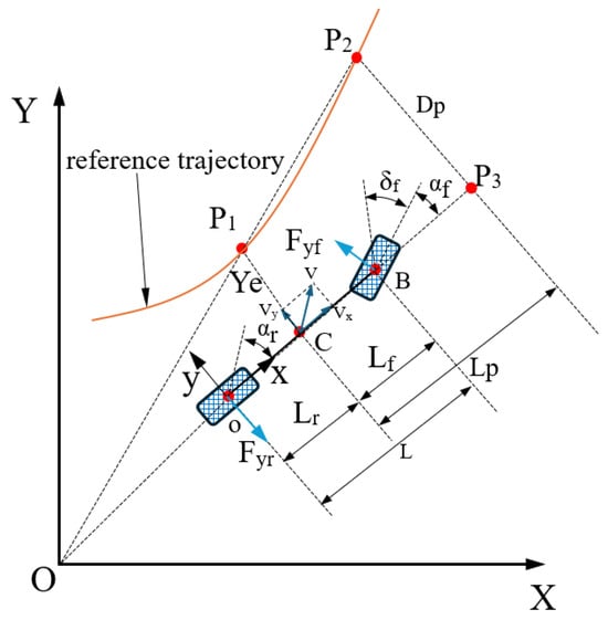
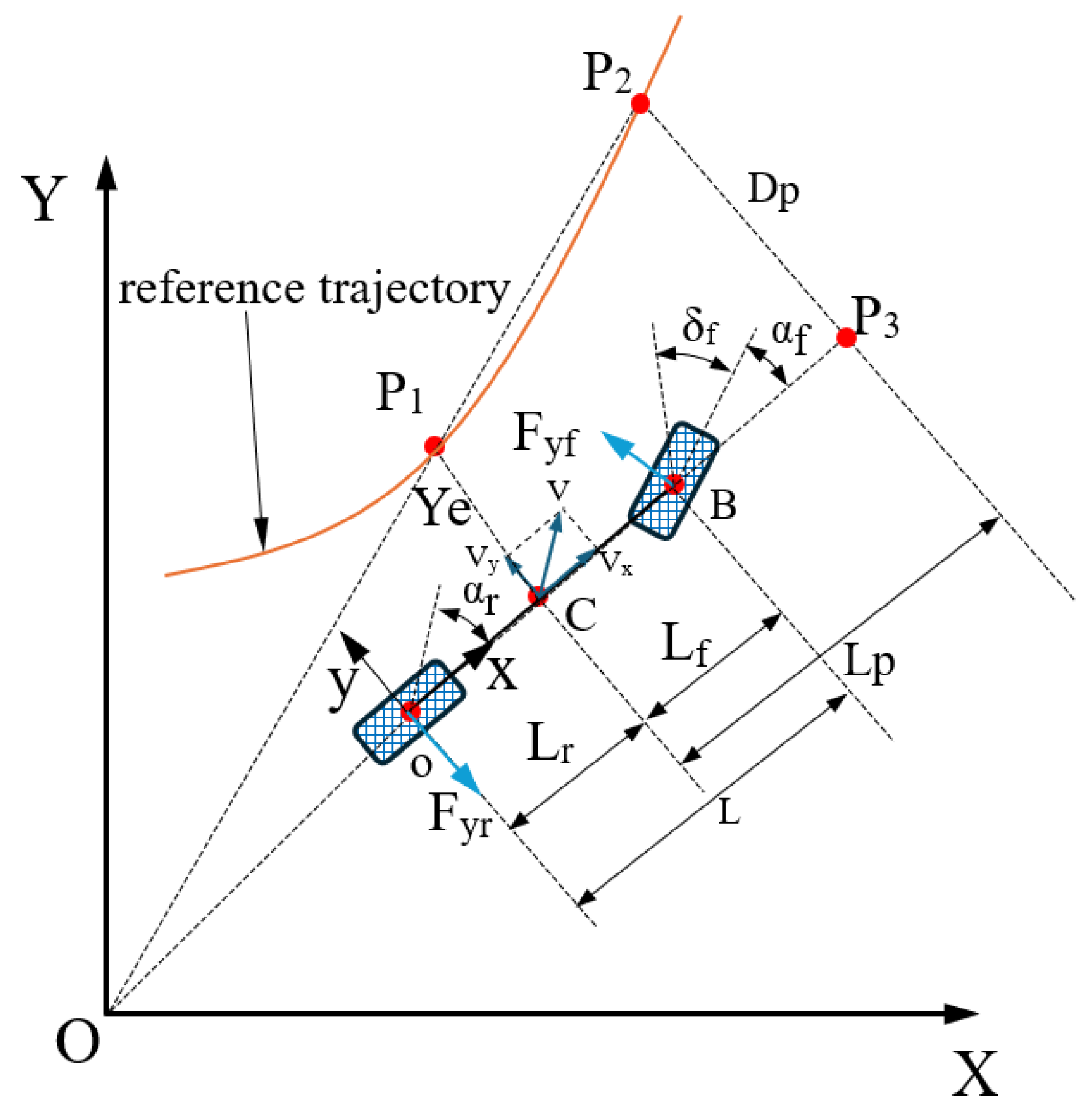
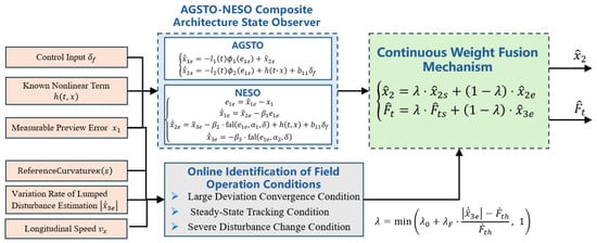
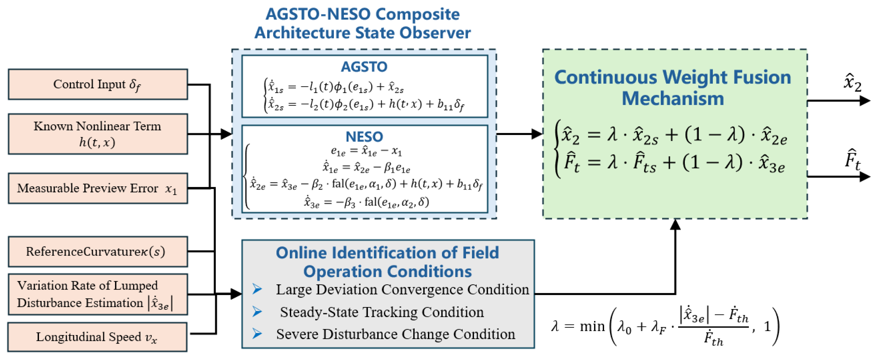
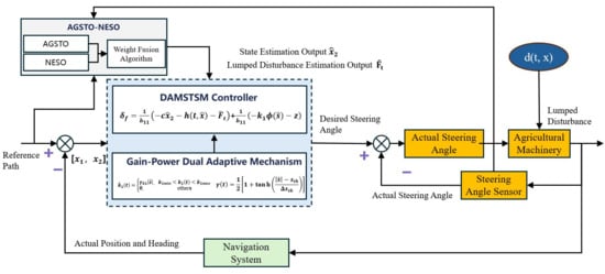
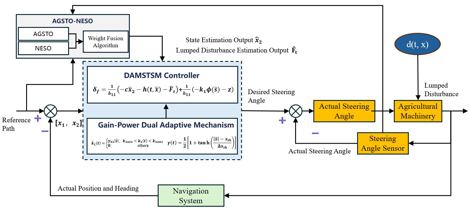
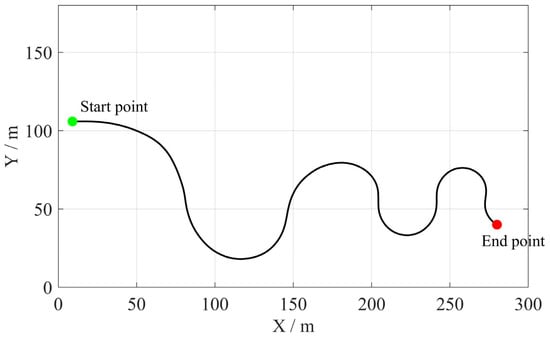
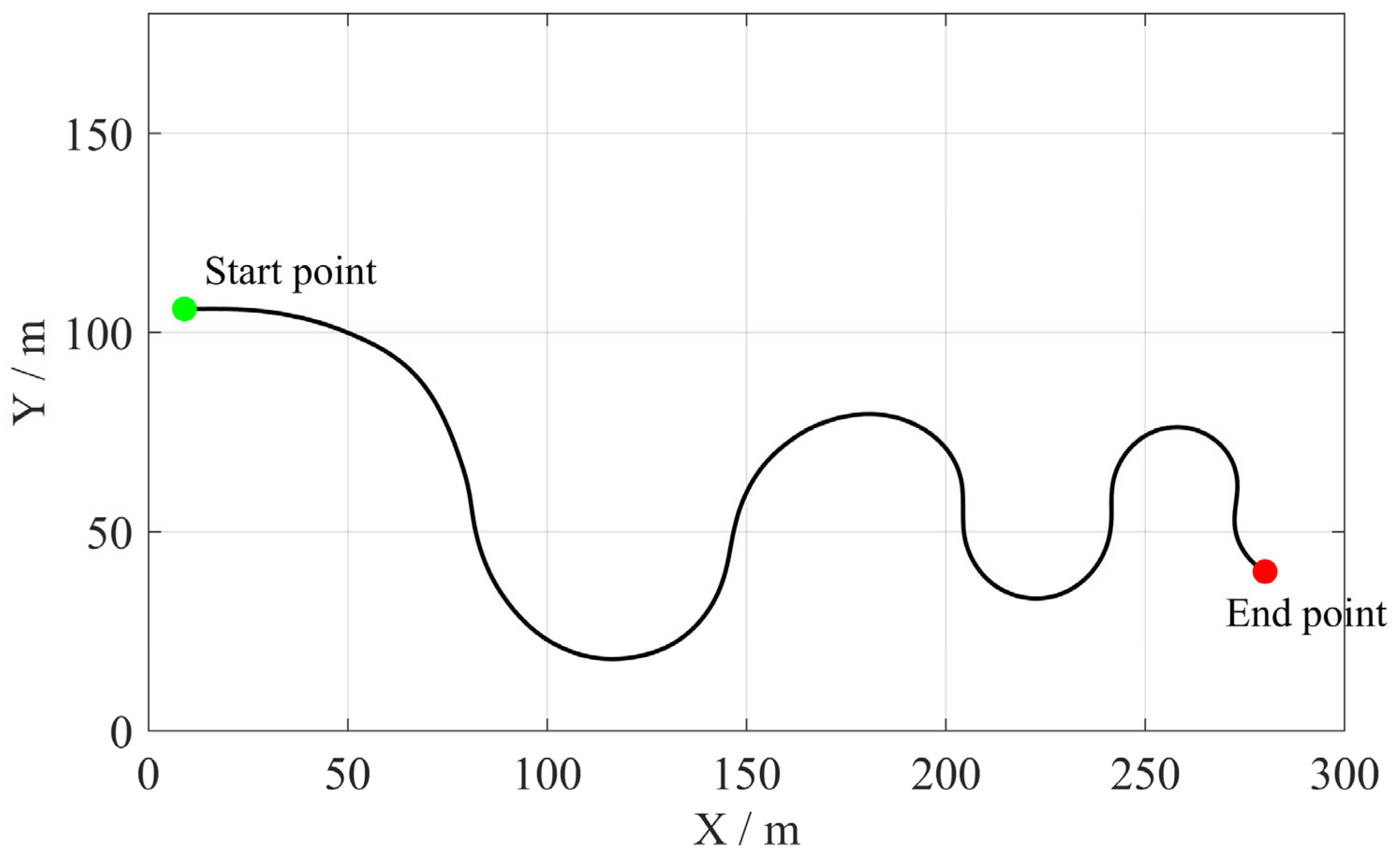
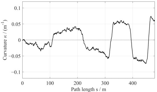
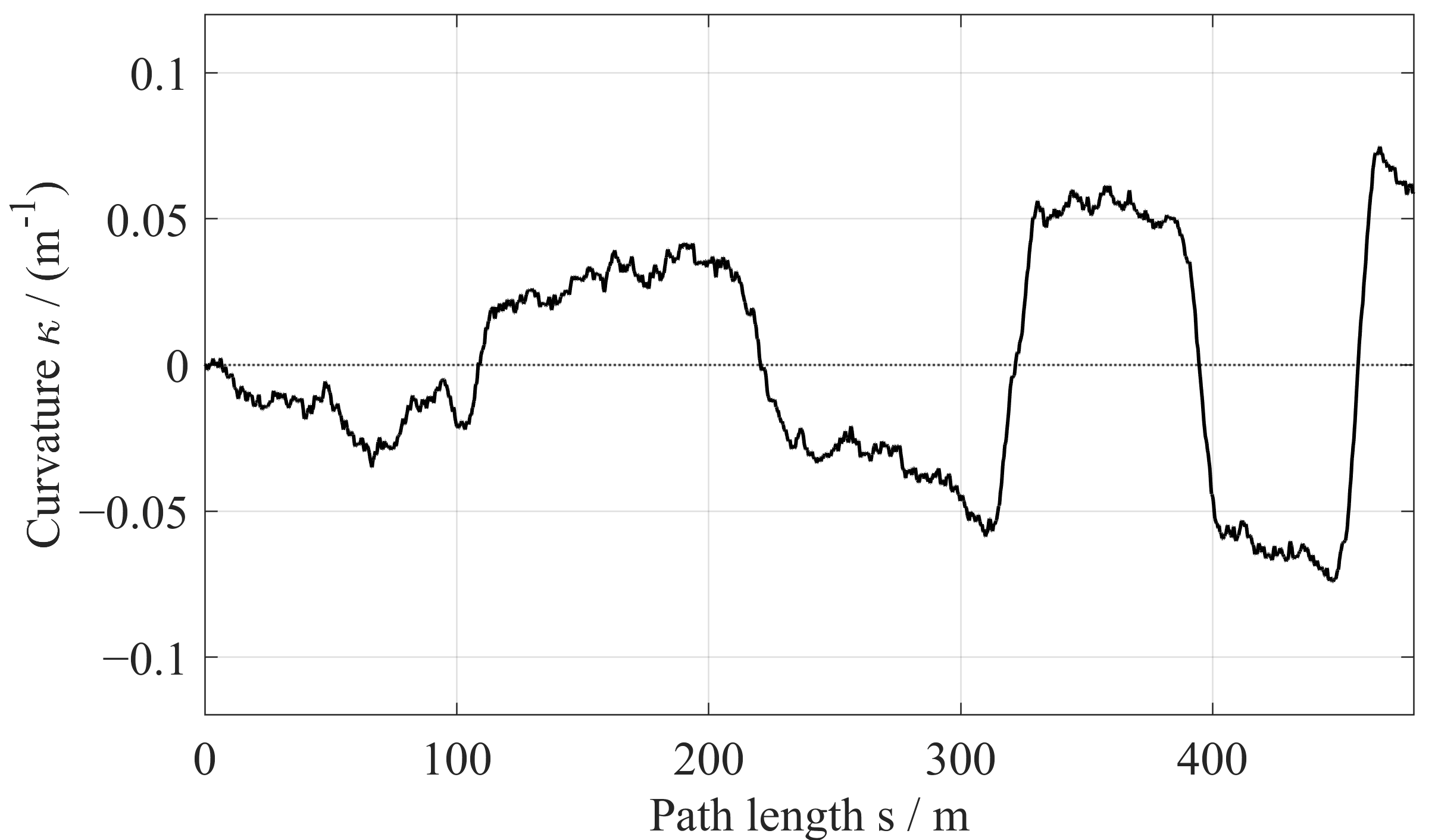
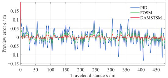
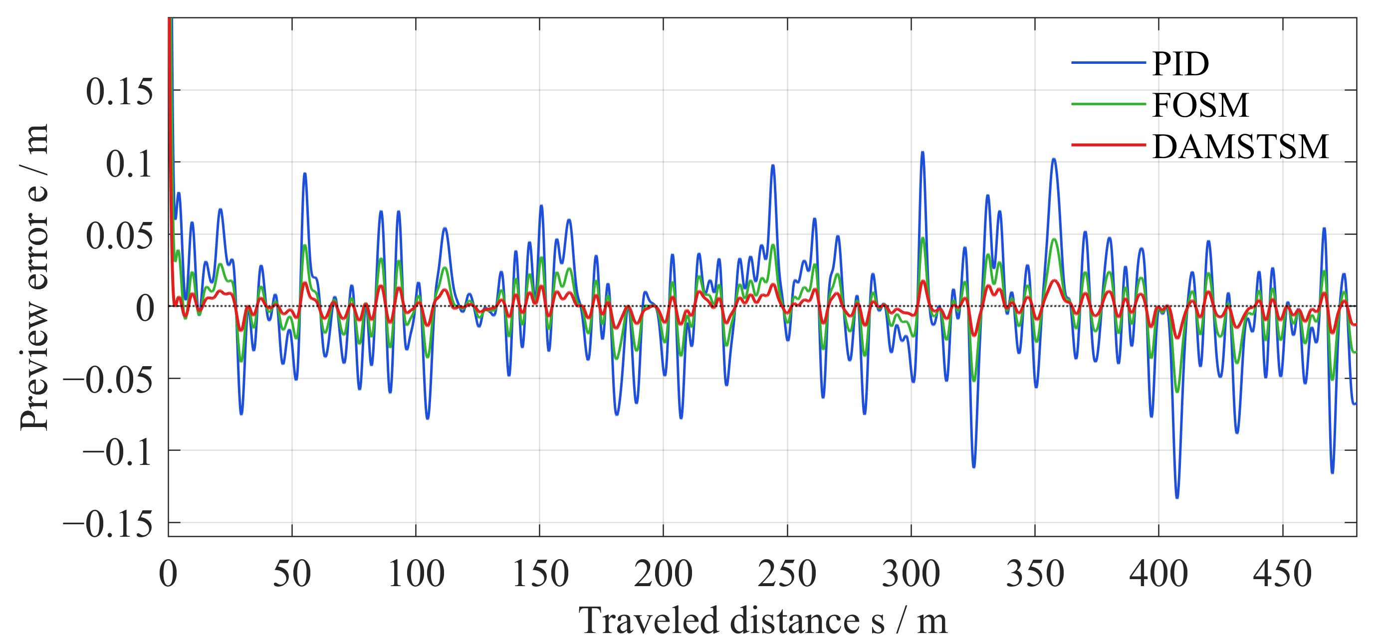
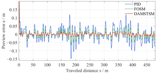
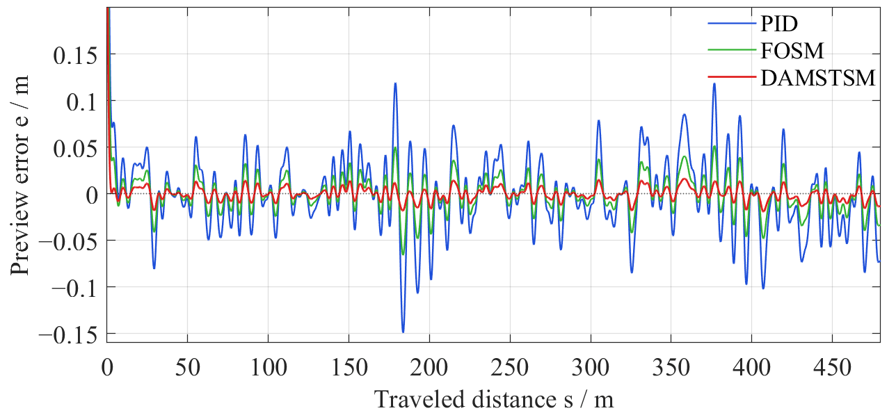
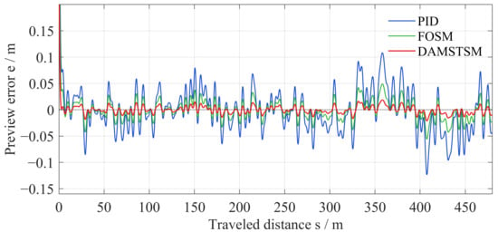
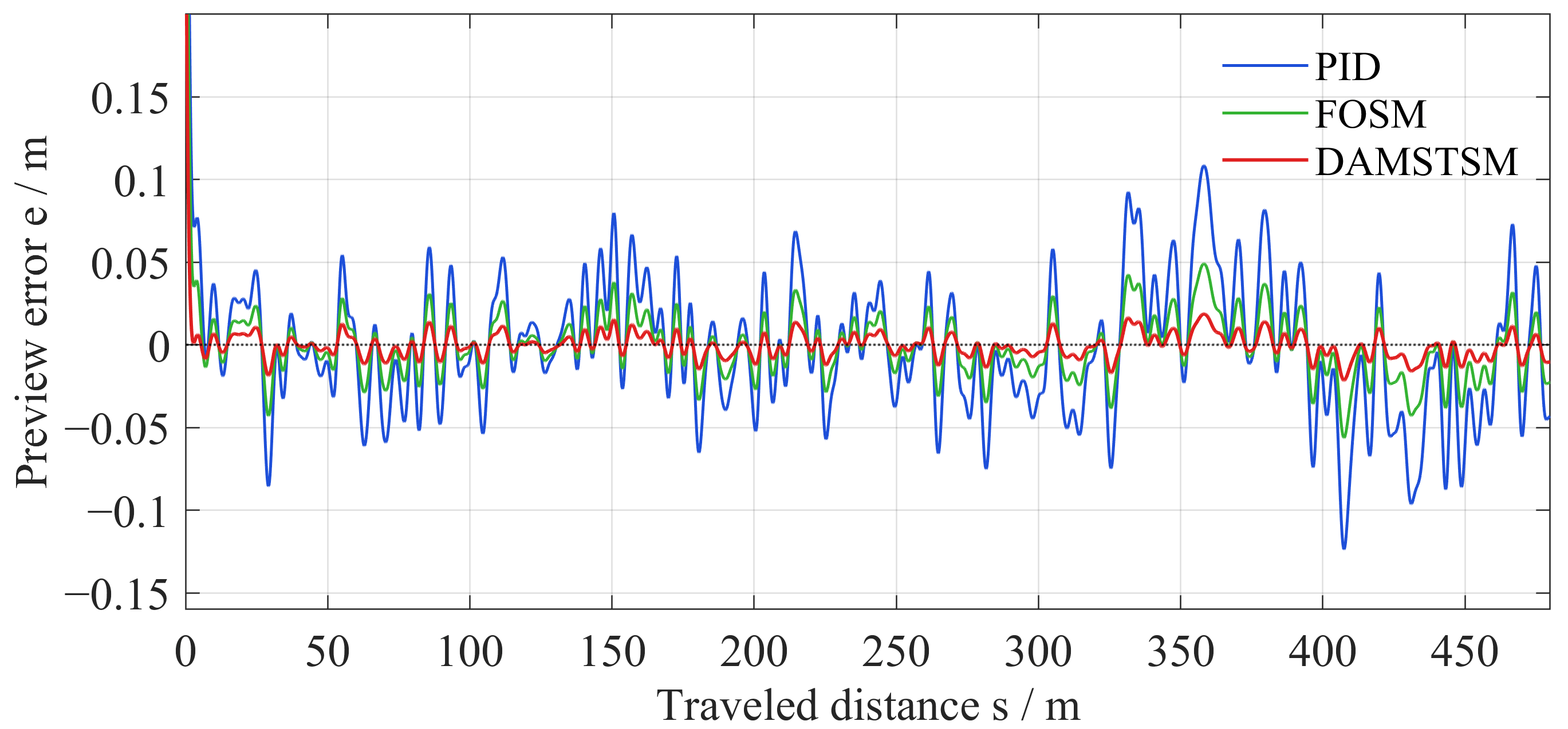
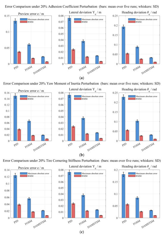
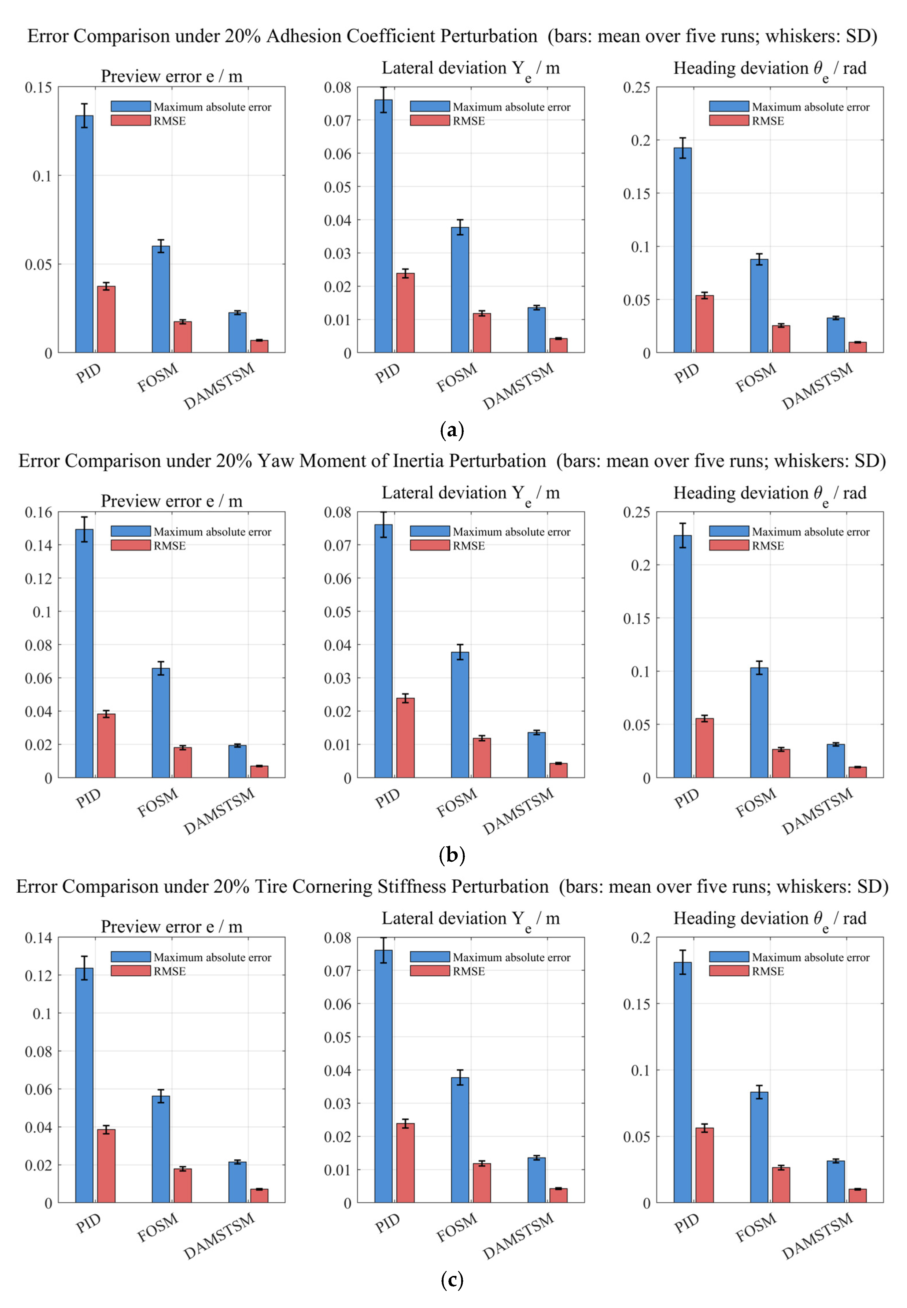
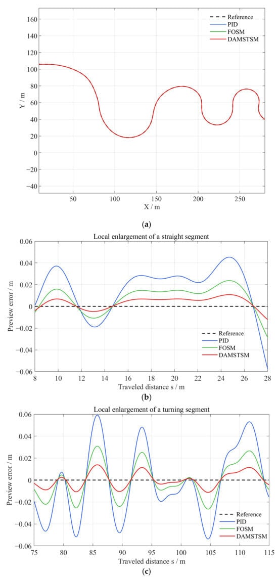
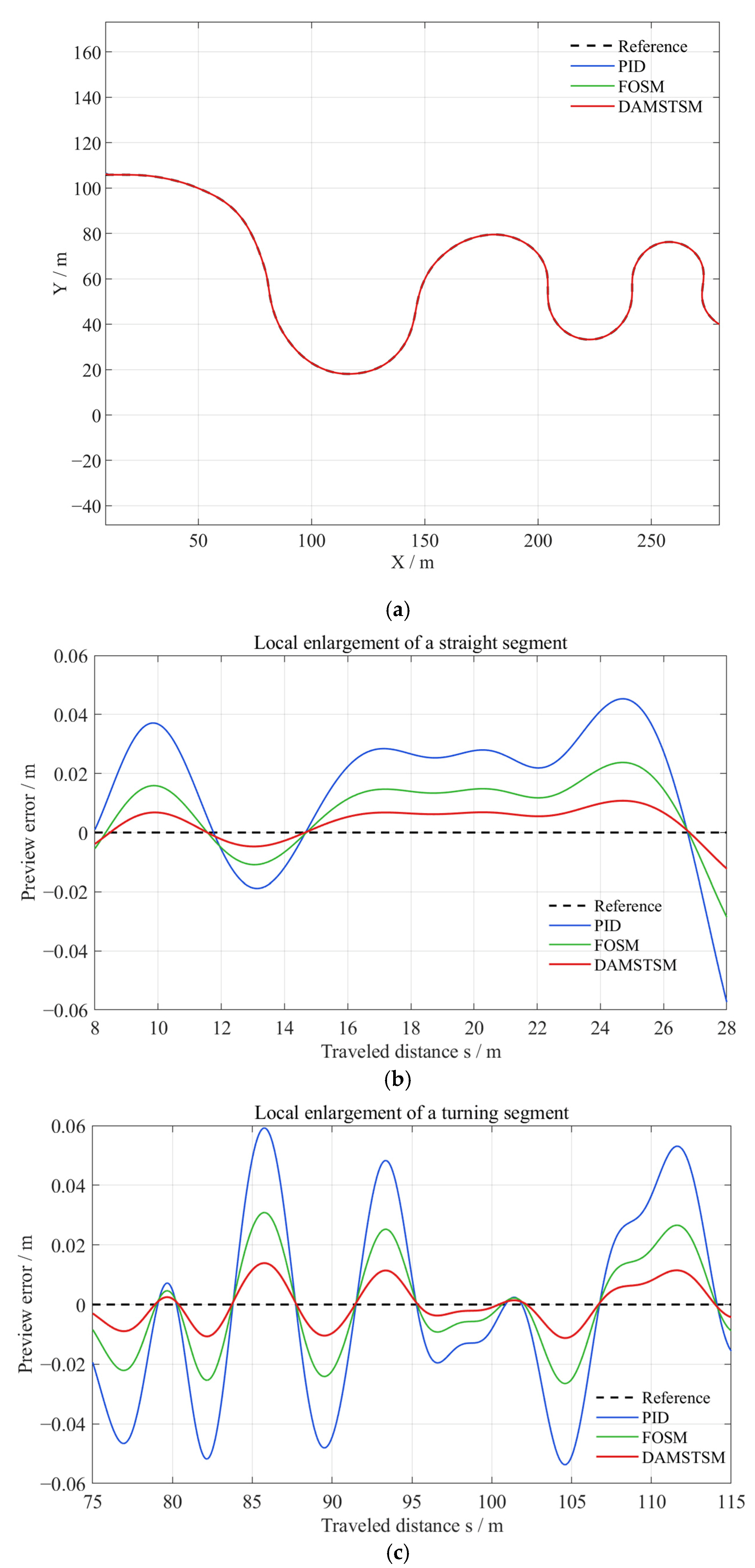
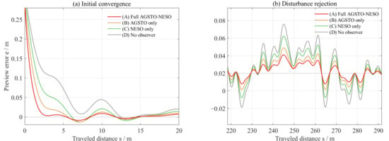
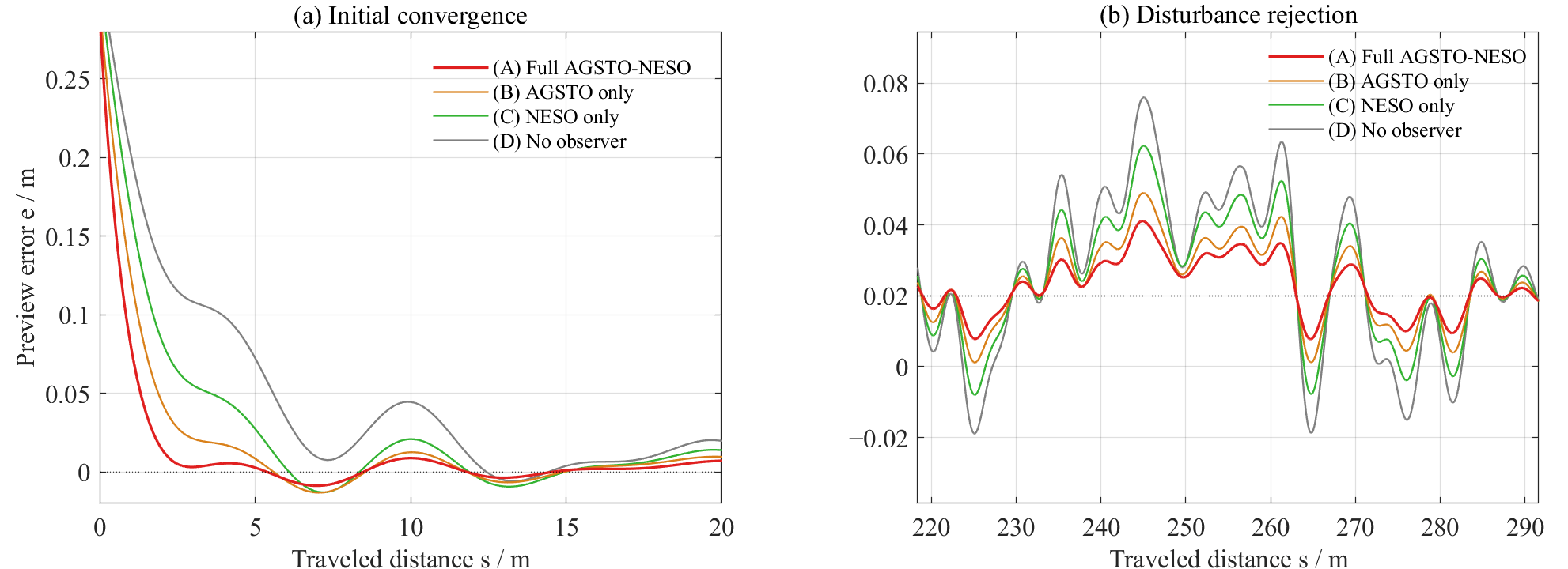
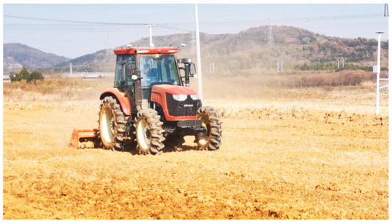
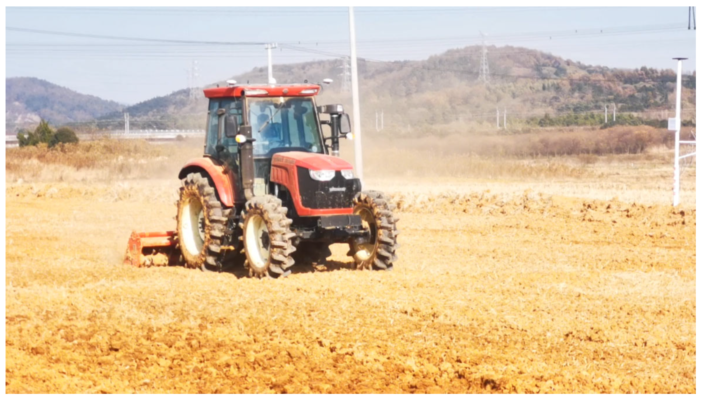
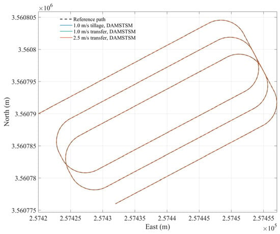
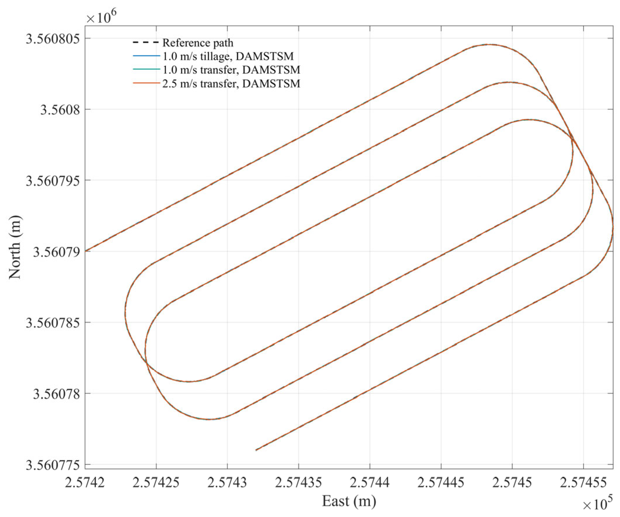
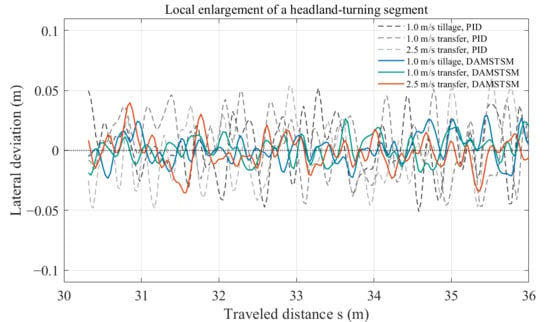
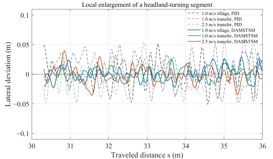
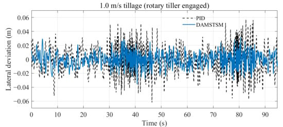
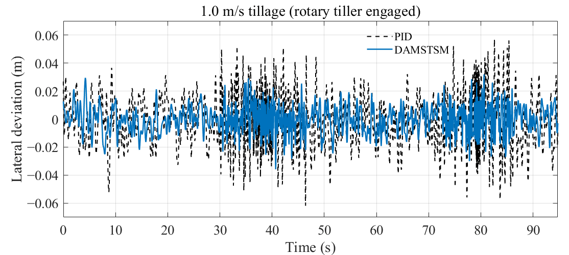
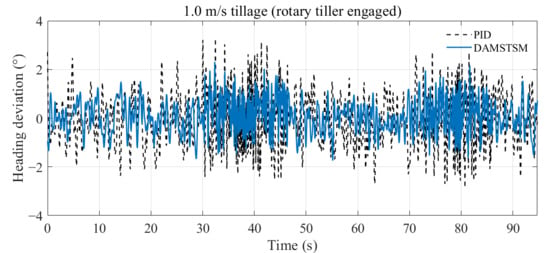
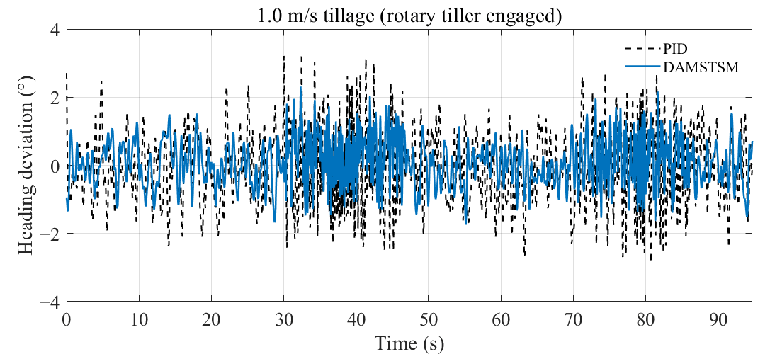
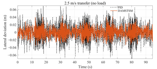
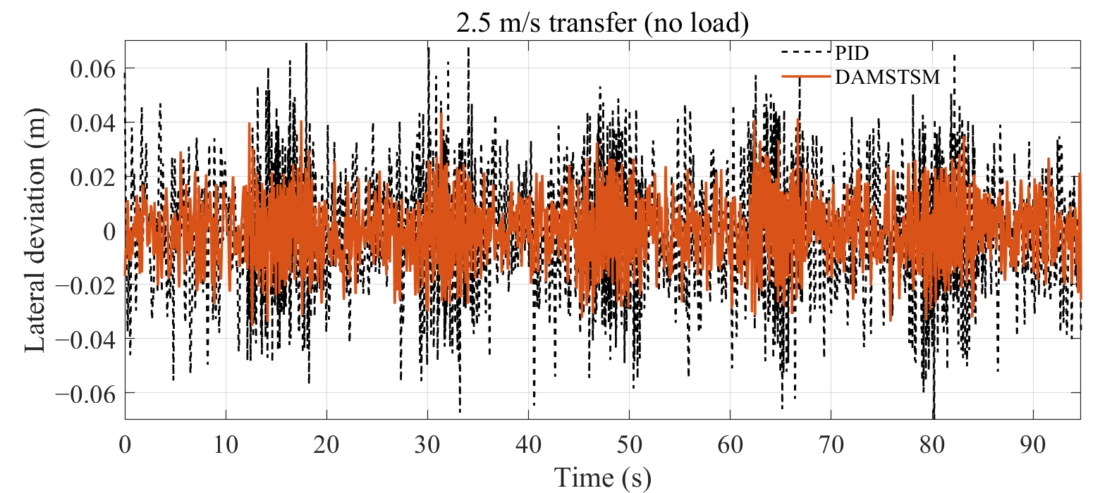
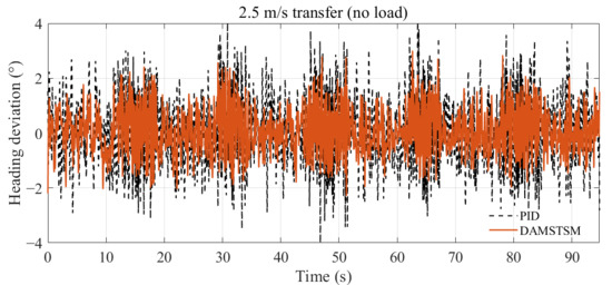
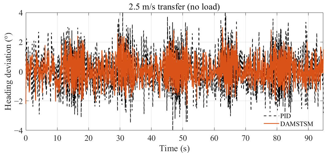
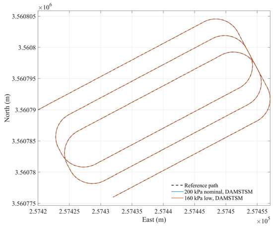
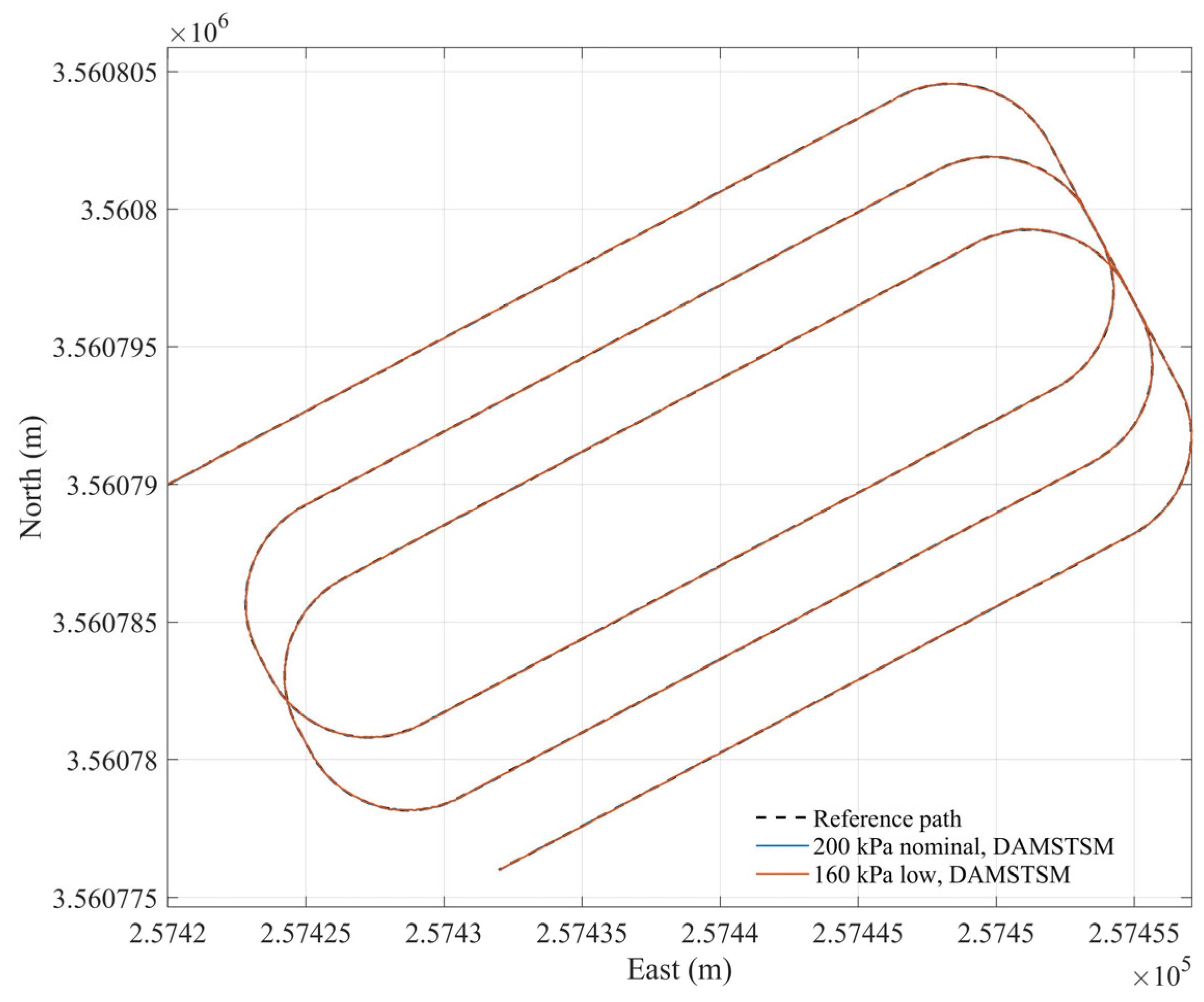
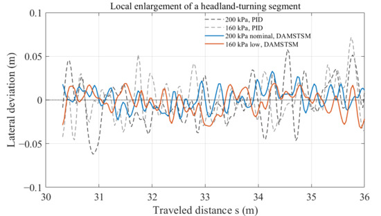
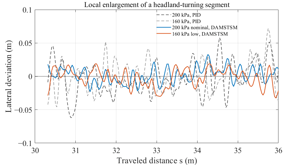
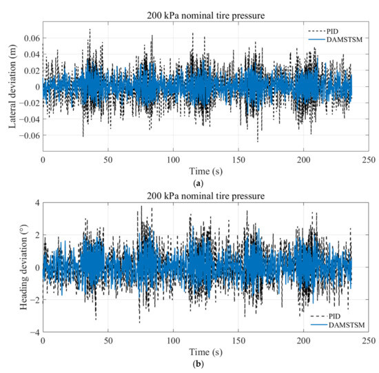
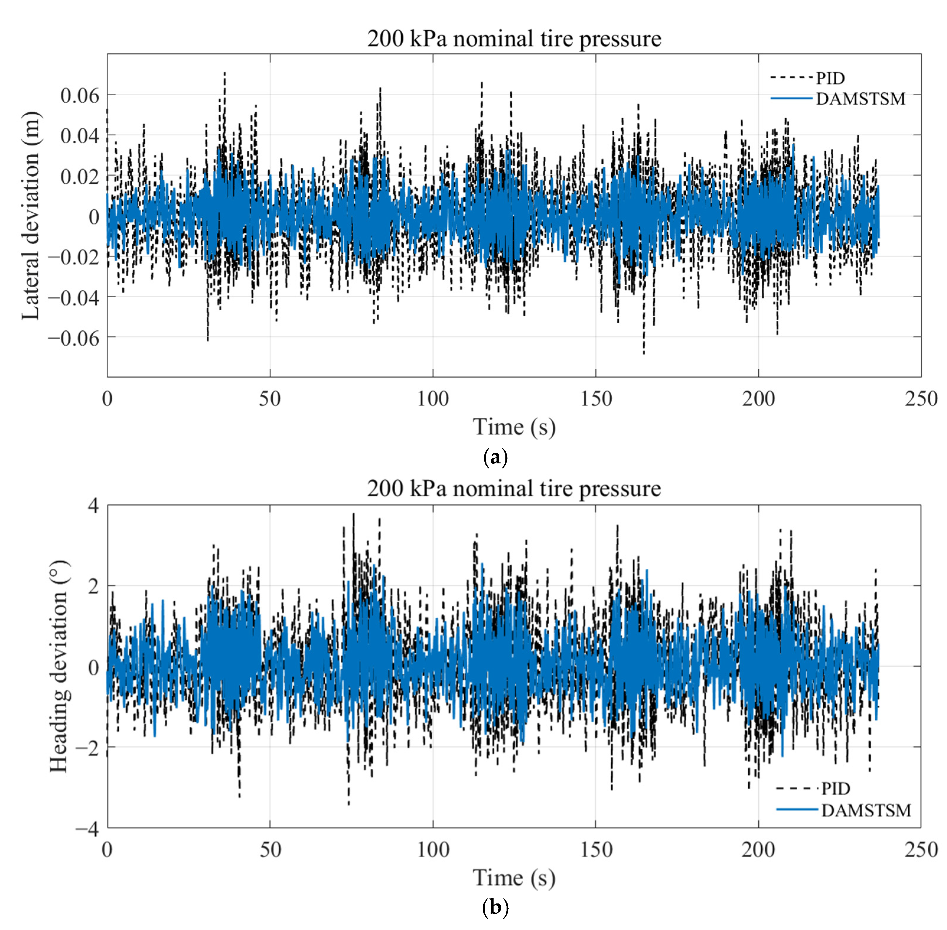
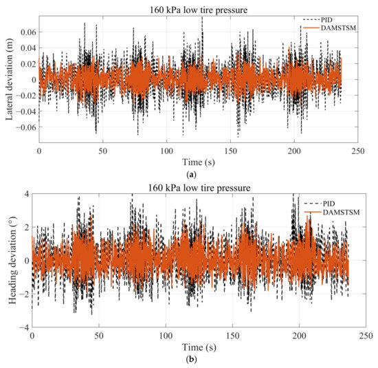
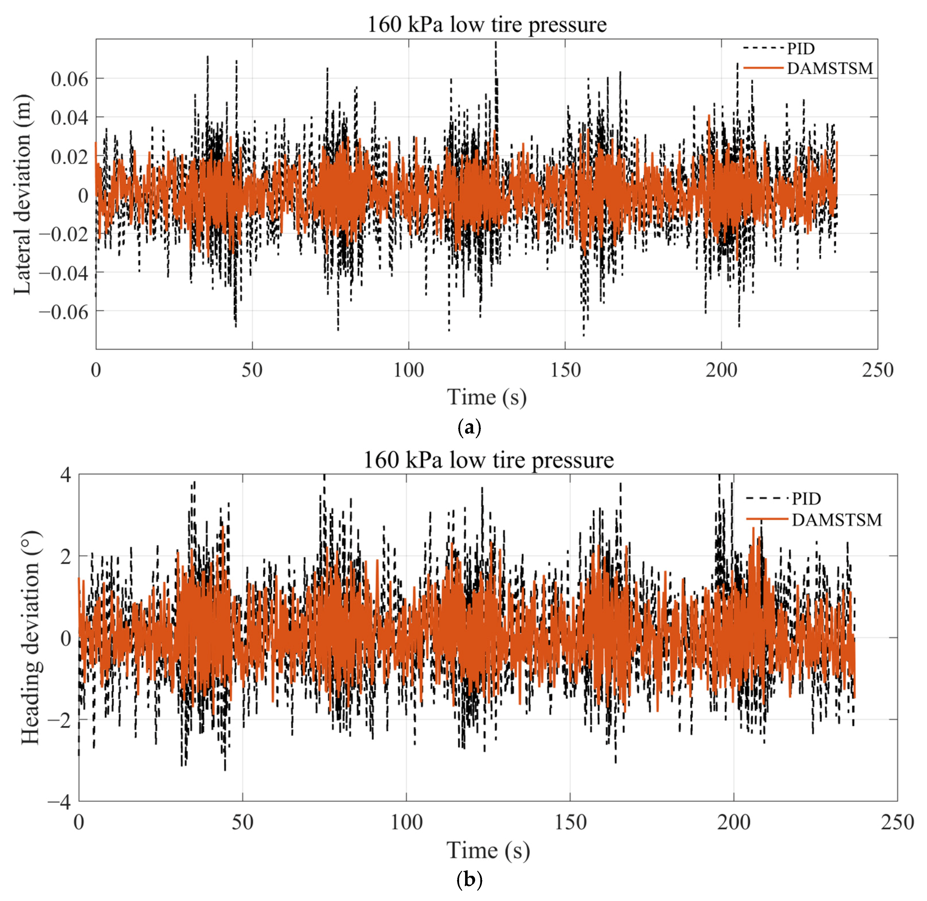

Disclaimer/Publisher’s Note: The statements, opinions and data contained in all publications are solely those of the individual author(s) and contributor(s) and not of MDPI and/or the editor(s). MDPI and/or the editor(s) disclaim responsibility for any injury to people or property resulting from any ideas, methods, instructions or products referred to in the content. |
© 2026 by the authors. Licensee MDPI, Basel, Switzerland. This article is an open access article distributed under the terms and conditions of the Creative Commons Attribution (CC BY) license.