Design and Experimental Validation of a DT-FPID-Based Local Canopy CO₂ Enrichment Control System in a Chinese Solar Greenhouse

Abstract

Carbon dioxide (CO₂) enrichment is an important means of increasing crop productivity in protected cultivation. However, local canopy CO₂ concentration in Chinese solar greenhouses is jointly affected by gas release, pipeline transport, and ventilation disturbances, making fixed-parameter proportional–integral–derivative (PID) control unable to simultaneously achieve rapid tracking, low overshoot, and fast disturbance recovery. This study developed a CO₂ enrichment system comprising controlled thermal decomposition of ammonium bicarbonate, condensation and water scrubbing, near-canopy delivery, and programmable logic controller (PLC)-based closed-loop control, and proposed a dynamic-target fuzzy PID (DT-FPID) strategy. Step-response tests were used to establish a first-order-plus-dead-time model linking heater duty cycle to local canopy CO₂ concentration, followed by fixed-target tracking, rule-based dynamic-target execution, and short-term ventilation-disturbance recovery tests in a local validation zone of a Chinese solar greenhouse. Relative to fixed-parameter PID, DT-FPID showed approximately 68–79% lower maximum overshoot and approximately 35–70% shorter ±20 ppm precision settling time (T₂₀) in simulation. At 600 ppm, the ±5% settling time was approximately 71% shorter, whereas at 800 and 1000 ppm it was broadly comparable to PID. In the greenhouse experiments, each controller–target combination included three independent runs. Based on descriptive comparisons of group means, DT-FPID showed approximately 47–49% lower mean maximum overshoot, approximately 36–40% shorter mean settling time, and approximately 77–80% shorter mean ventilation-disturbance recovery time; its mean maximum overshoot and settling time were also lower than those of conventional fuzzy PID. All three dynamic-target field runs completed the prescribed switches among the 600, 800, and 1000 ppm target levels. These results support control performance only under the short-term local validation conditions of this study; they are not used to determine physiologically or economically optimal CO₂ concentrations or to extrapolate whole-greenhouse uniformity or long-term production effects.

1. Introduction

Southern Xinjiang has abundant solar and thermal resources. Using yellow sand as a cultivation substrate in Chinese solar greenhouses can reduce reliance on conventional arable soil and improve the crop root-zone environment. Song et al. demonstrated that water and fertilizer management regulates photosynthetic performance, dry-matter accumulation, and yield of tomato grown in a yellow-sand substrate [1]. However, root-zone water and nutrient management does not directly replenish the carbon source required for canopy photosynthesis. Once the tomato canopy develops, daytime photosynthesis continuously consumes greenhouse CO₂, while structural leakage and ventilation further intensify gas losses, leading to CO₂ depletion near the canopy. Wang et al. reviewed greenhouse CO₂ enrichment and showed that its effectiveness is jointly influenced by ventilation, weather conditions, and crop growth status [2]. Li et al. summarized automatic CO₂ enrichment strategies and emphasized that supply timing and concentration control should be adjusted in response to environmental variation [3]. Kuroyanagi et al. used a mass-balance analysis to show that substantial CO₂ losses can occur through structural leakage even without active ventilation [4]. Therefore, CO₂ regulation in Chinese solar greenhouses requires not only adequate carbon supply to the canopy but also rational target generation and stable target execution under changing environmental conditions.

The performance of a CO₂ enrichment system is also affected by gas-release characteristics, gas purification, and the delivery position. Li et al. compared multiple CO₂ enrichment technologies in terms of energy consumption and cost [5]. Villagran et al. systematically reviewed gas sources, purification, delivery, and environmental control in protected-cultivation CO₂ enrichment systems [6]. Resentera et al. confirmed that thermal decomposition of ammonium bicarbonate produces CO₂, NH₃, and water vapor, and that the decomposition process is affected by temperature and reaction conditions [7]. CFD analysis coupled with a photosynthesis model by Zhang et al. showed that different enrichment methods generate markedly different spatial distributions of greenhouse CO₂ [8]. Kimura et al. reported significant spatiotemporal variability in both greenhouse microclimate and leaf photosynthetic rate [9]. Hidaka et al. demonstrated that crop-local CO₂ enrichment can increase strawberry yield and fuel-use efficiency [10]. Mochizuki et al. further found that within-canopy CO₂ application increases strawberry dry-matter production and fruit yield [11].

CO₂ enrichment processes exhibit inertia, dead time, operating-point variation, output saturation, and ventilation disturbances. Consequently, conventional fixed-parameter controllers often cannot simultaneously achieve rapid response, overshoot suppression, and smooth actuation. Chen et al. used nonlinear model predictive control (NMPC) to address multivariable interactions and actuator constraints in a semi-closed greenhouse, demonstrating that process modeling and constraint handling are essential for improving greenhouse control performance [12]. Li et al. improved greenhouse environmental regulation through predictive compensation and fuzzy gain tuning [13]. Song et al. verified the feasibility of fuzzy PID control in a solid-fertilizer-dissolving device [14]. Xu et al. combined system identification with fuzzy PID control to improve the dynamic performance of real-time EC regulation during fertilizer mixing [15].

In addition to closed-loop execution performance, the CO₂ target concentration should not remain constant under continuously changing greenhouse conditions. Sánchez-Guerrero et al. found that variable CO₂ enrichment can adjust the supply level to greenhouse operating conditions and improve radiation-use efficiency [16]. Gao et al. incorporated irradiance, photosynthetic rate, and CO₂ cost into target optimization, indicating that the target concentration should balance environmental conditions, crop response, and operating cost [17]. Su and Xu noted that greenhouse setpoint optimization requires a trade-off between energy consumption and crop production [18]. Zhang et al. found that the photosynthetic response of greenhouse tomato leaves varies with CO₂ concentration [19]. Kläring et al. used a crop model to regulate greenhouse CO₂ concentration, providing a basis for crop-response-based adjustment of CO₂ setpoints [20].

Against this background, this study focused on the development of a local canopy CO₂ enrichment system, process identification, and closed-loop validation. A CO₂ enrichment system integrating controlled ammonium bicarbonate gas release, condensation, water scrubbing and demisting, near-canopy delivery, PLC feedback control, and safety interlocks was developed. Step-response tests were used to identify the dynamic relationship between heater duty cycle and local canopy CO₂ concentration and to establish an FOPDT nominal model for uniform controller comparison. A dynamic-target-coupled fuzzy PID strategy was then constructed by adding a tiered-target generator based on predefined environmental rules, integral attenuation, a proportional soft dead zone, error zero-crossing handling, and an output-rate limit to conventional fuzzy PID. Finally, fixed- and dynamic-target simulations, together with greenhouse tests of fixed-target tracking, dynamic-target execution, and recovery from short-term ventilation disturbances, were conducted to evaluate target tracking, tiered-target execution, and disturbance recovery.

2. Materials and Methods

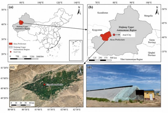
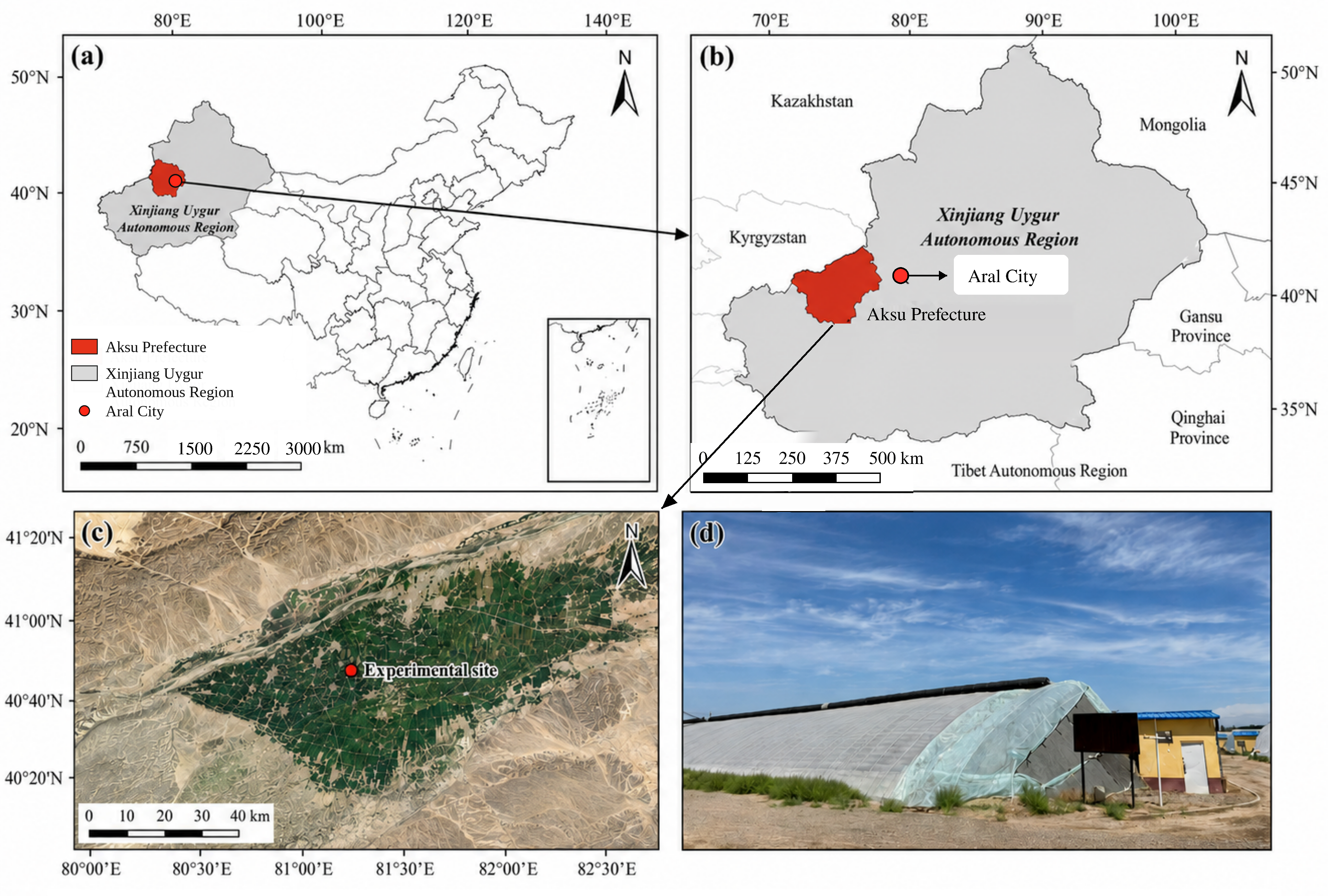
The experiments were conducted in Alar City, Xinjiang Uygur Autonomous Region, China. The regional and site locations are shown in Figure 1.

Figure 1. Location of the experimental site. (a) Location of the Xinjiang Uygur Autonomous Region and Alar City in China; (b) location of Alar City within Xinjiang; (c) satellite image of the experimental area; and (d) exterior view of the experimental Chinese solar greenhouse. Panels (a,b) were prepared by the authors using ArcGIS Pro 3.7.1 (Esri, Redlands, CA, USA). The satellite image in panel (c) was obtained from Google Earth Pro 7.3.7 (Google LLC, Mountain View, CA, USA) on 27 July 2026, with the original Google and imagery-provider attribution retained. The photograph in panel (d) was taken by the authors in May 2026.

2.1. CO₂ Enrichment System Design and Operating Principle

2.1.1. Overall System Architecture

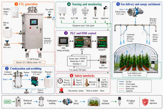
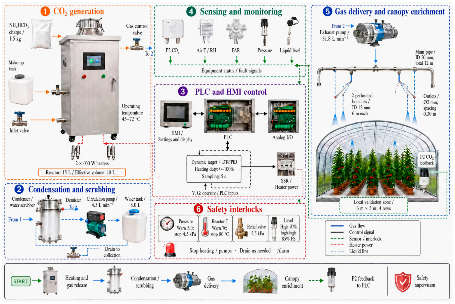
To achieve stable local canopy CO₂ supply, feedback regulation, and safe operation in a Chinese solar greenhouse, a CO₂ enrichment system using controlled ammonium bicarbonate gas release as the gas source was developed. The system comprised six functional modules: CO₂ generation, condensation and water scrubbing, sensing and monitoring, control and human–machine interaction, gas delivery and local canopy enrichment, and safety interlocking. The system architecture and signal relationships are shown in Figure 2, and the main hardware specifications are listed in Table 1.

Figure 2. Architecture and operating principle of the prototype CO₂ enrichment system in the Chinese solar greenhouse. 1, CO₂ generation module; 2, condensation and water-scrubbing module; 3, control and human–machine interface module; 4, sensing and monitoring module; 5, gas-delivery and local canopy enrichment module; 6, safety-interlock module.

Table 1. Main hardware components and technical specifications of the CO₂ enrichment system.

No.	Component	Model	Main Technical Specifications
1	Sealed gas-generation reactor	Custom-built	Total volume, 15 L; effective loading volume, 10 L; SUS304 stainless steel; wall thickness, 1.5 mm
2	Cartridge heaters	Custom-integrated	2 × 600 W; 220 V; total rated power, 1200 W
3	Solid-state relay	NJG1 (Zhejiang CHINT Electrics Co., Ltd., Yueqing, China)	Receives the PLC time-proportional signal and switches the heaters
4	NDIR CO2 sensor	CM1106H-NS (Cubic Sensor and Instrument Co., Ltd., Wuhan, China)	Accuracy: ± 30 ppm + 3% of reading
5	Temperature–humidity transmitter	RS-WS series (Shandong Renke Control Technology Co., Ltd., Jinan, China)	Temperature accuracy: ± 0.5 °C; relative-humidity accuracy: ± 3% RH
6	Photosynthetically active radiation sensor	RS-GH series (Shandong Renke Control Technology Co., Ltd., Jinan, China)	Accuracy: ± 5%
7	Non-contact liquid-level sensor	XKC-Y28A (Shenzhen XingKeChuang Technology Co., Ltd., Shenzhen, China)	Liquid-level detection accuracy: ±1.5 mm
8	Micropressure transmitter	MPM430 (Micro Sensor Co., Ltd., Baoji, China)	Monitors reactor and pipeline pressure; range, accuracy, and calibration information are provided in Supplementary Table S2
9	Programmable logic controller	XD series (Wuxi Xinje Electric Co., Ltd., Wuxi, China)	Data acquisition, control computation, and equipment interlocking
10	Analog input/output module	XD-E4AD2DA (Wuxi Xinje Electric Co., Ltd., Wuxi, China)	Analog input resolution: 14 bit
11	Normally closed two-way solenoid valve	2W series	On/off control of gas and liquid lines
12	Exhaust pump	—	Rated flow rate: 35 L·min−1; measured operating flow rate: 31.8 L·min−1
13	Condensation and water-scrubbing unit	Custom-integrated	Recirculating-tank working volume: 8.0 L; recirculation-pump rated flow: 4.5 L·min−1
14	Local gas-delivery pipeline	Custom-built	Main-pipe internal diameter: 20 mm; total length: 12 m; two branch pipes, internal diameter 12 mm and length 6.0 m each; outlet-hole diameter: 2.0 mm; hole spacing: 0.3 m
15	Demister	Custom-integrated	Installed downstream of the condensation and scrubbing unit to remove entrained droplets
16	Mechanical pressure-relief valve	—	Independent mechanical overpressure protection; opening pressure: 5.5 kPa

2.1.2. Operating Principle

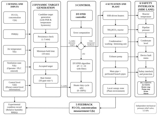
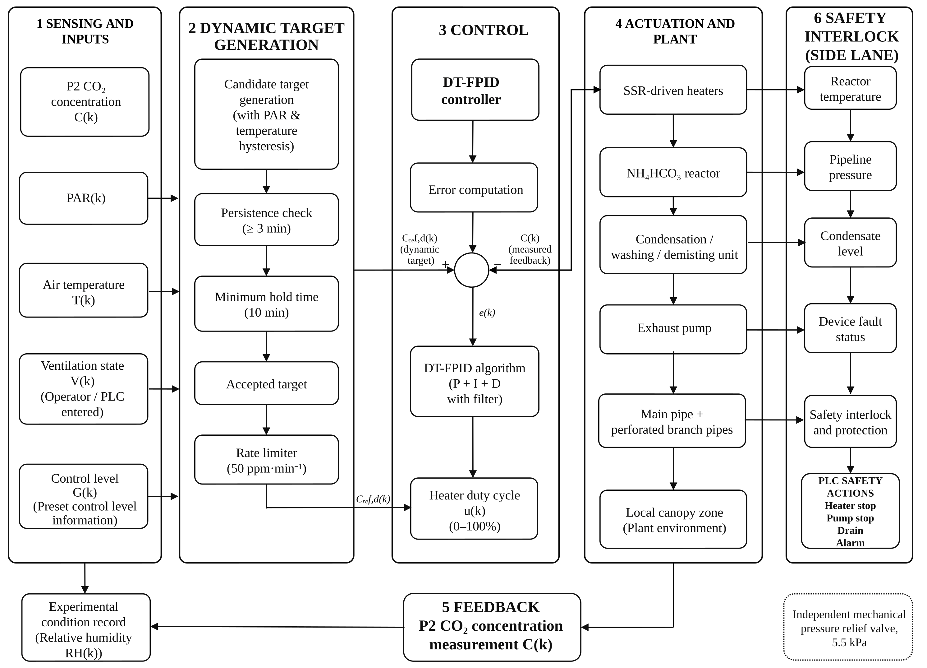
The system workflow is illustrated in Figure 3. During operation, the P2 sensor measured CO₂ concentration near the tomato canopy in real time. The PLC calculated the heater duty cycle from the deviation between the reference and measured concentrations, and a solid-state relay regulated the on/off operation of the cartridge heaters in the reactor. After approximately 1.5 kg of ammonium bicarbonate was loaded into the reactor, the heaters, with a total rated power of 1200 W, were activated and the reactor operating temperature was maintained at 45–72 °C. The generated gas mixture then passed through condensation, water scrubbing, and demisting before being conveyed by the exhaust pump to the main pipe and perforated branch pipes installed along the crop rows, where it was released near the canopy. The P2 measurement was returned to the PLC, thereby forming a closed loop with local canopy CO₂ concentration as the feedback variable and heater duty cycle as the manipulated variable.

Figure 3. Closed-loop control model of the CO₂ enrichment system.

Under normal equipment status, the control system operated with a sampling period of 5 s and selected either a fixed or a dynamic reference according to the test mode. In fixed-target mode, the prescribed C_ref(k) bypassed the dynamic-target generator. In dynamic-target mode, the rule-based generator used PAR(k), air temperature T(k), ventilation state V(k), and control level G(k) to produce C_ref,d(k), with persistence checking, a minimum hold time, hysteresis, and a target-rate limit. V(k) and G(k) represented ventilation-state and control-setting information rather than additional environmental sensor measurements. The controller then generated a 0–100% heater duty cycle u(k) from the selected reference. Pressure, liquid level, and equipment status were used for safety-interlock decisions. The PLC alarm and shutdown thresholds for reactor temperature were 76 and 80 °C, respectively; the pipeline-pressure warning and shutdown thresholds were 3.0 and 4.5 kPa; the high- and high-high-condensate-level thresholds were 70% and 85% of full scale, respectively; and the mechanical pressure-relief valve opened at 5.5 kPa. When a parameter exceeded its limit, communication was interrupted, or an actuator failed, the system stopped heating and pumping, initiated drainage, and issued an alarm.

Thermal decomposition of ammonium bicarbonate releases CO₂, NH₃, and H₂O [7]. The removal efficiency of NH₃ by spray wet scrubbing is affected by gas–liquid contact and operating parameters [21]. To characterize the reduction of co-generated NH₃ by condensation and water scrubbing during short-term operation, NH₃ signals were measured upstream of the scrubber, downstream of the scrubber, and at P2 at heater duty cycles of 40%, 60%, 80%, and 100%, with three replicates per condition. The detection configuration and screening results are presented in Supplementary Table S2. The sub-ppm readings at P2 were used only as low-level screening signals and not to assess long-term exposure or operational safety.

2.2. Controller Design

2.2.1. PID Control

A positional fixed-parameter PID controller was established as the baseline, with the deviation between the target concentration and the P2 measurement as the input and heater duty cycle as the output. The concentration error at sampling instant k was defined as follows:

e(k) = C_ref(k) − C(k)

(1)

where C_ref(k) is the reference concentration and C(k) is the CO₂ concentration measured at P2. The discrete integral-state update, operating-point feedforward term, and positional PID output were defined as follows:

$$I_e\left(k\right)=I_e\left(k-1\right)+e\left(k\right)\Delta t$$

(2)

$$u_b\left(k\right)=u_0+{\displaystyle \frac{C_{ref}\left(k\right)-C_0}{K}}$$

(3)

$$u\left(k\right)=\mathit{s}\mathit{a}\mathit{t}\left\{u_b\left(k\right)+K_{p}e\left(k\right)+K_i{I}_e\left(k\right)-K_d{d}_f\left(k\right), 0, 100\right\}$$

(4)

where u(k) is the heater duty cycle; sat(·, 0, 100) limits the output to 0–100%; and K_p, K_i, and K_d are the proportional, integral, and derivative gains, respectively. The derivative term acted on the measured concentration rather than on the reference to reduce derivative kick during target switching. The measured concentration rate was d_m(k) = [C(k) − C(k − 1)]/Δt and was filtered as d_f(k) = 0.20dm(k) + 0.80d_f(k − 1).

The sampling interval Δt was 5/60 min. The operating-point duty cycle u₀, background concentration C₀, and nominal static gain K were 20%, 390.833 ppm, and 10.1204 ppm·%⁻¹, respectively. Unless otherwise specified, all three controllers used the same operating-point feedforward term, baseline PID gains, 0–100% output saturation, and conditional integration anti-windup rule. Conditional integration prevents continued accumulation of the integral term while the actuator is saturated [22].

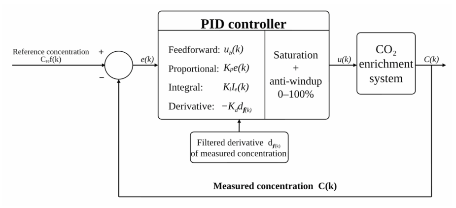
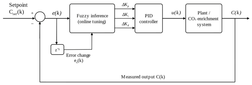
After the integral candidate was formed and the current control command was calculated, the applicable duty-step limit and 0–100% saturation were imposed. If the final output was at the upper limit with a positive error, or at the lower limit with a negative error, the current integral increment was not retained; otherwise, the integral candidate was accepted. This conditional state update affected subsequent samples and did not trigger recalculation of the current limited output. The baseline proportional, integral, and derivative gains were 0.20%·ppm⁻¹, 0.05%·ppm⁻¹·min⁻¹, and 0.15%·min·ppm⁻¹, respectively. The baseline PID parameters, fuzzy-tuning parameters, and DT-FPID constraint-layer parameters used for formal performance evaluation were all determined and locked before the formal field evaluation began and were not readjusted on the basis of the evaluation results. The parameter search ranges, final values, and related settings are provided in Table A1, and the fuzzy quantization and rule parameters are given in Table A2 and Table A3. The fixed-parameter PID control principle is illustrated in Figure 4.

Figure 4. Fixed-parameter PID control principle.

Figure 4. Fixed-parameter PID control principle.

2.2.2. Fuzzy PID Control

To improve adaptation to variations in gas-release conditions, transport delay, and ventilation loss, a conventional fuzzy PID controller was constructed on the fixed-parameter PID baseline. The controller used the concentration error e(k) and per-sample error increment e_c(k) = e(k) − e(k − 1) as inputs, which were quantized and mapped to the universe of discourse [−6, 6]:

$$\begin{gathered} E\left(k\right)=\mathit{s}\mathit{a}\mathit{t}\left[-K_{e}e\left(k\right), -6, 6\right] \\ \mathit{E}\mathit{C}\left(k\right)=\mathit{s}\mathit{a}\mathit{t}\left[-K_{ec}ec\left(k\right), -6, 6\right] \end{gathered}$$

(5)

where E(k) and E_C(k) are the quantized error and error increment, respectively, and the quantization factors K_e and K_ec were 0.010 and 0.120. Because the rule base adopted the sign convention “measured value minus reference value”, the signs of both the error and its increment were inverted before fuzzy inference.

Both E and E_C were partitioned into seven linguistic variables: NB, NM, NS, ZO, PS, PM, and PB. Trapezoidal membership functions were used at the two extremes and triangular membership functions for the intermediate sets. Parameter tuning used a seven-level fuzzy rule base. Rule outputs were membership-weighted to obtain real-time corrections to the proportional, integral, and derivative gains, ΔK_p(k), ΔK_i(k), and ΔK_d(k), respectively. Their maximum magnitudes were 0.035, 0.010, and 0.300. Complete membership-function parameters and the 7 × 7 rule bases are provided in Table A2 and Table A3.

The PID gains were updated online as follows:

$$\begin{gathered} K_{\mathrm{p}}\left(k\right)=K_{\mathrm{p}0}+\Delta K_{\mathrm{p}}\left(k\right) \\ {K}_{\mathrm{i}}\left(k\right)=K_{\mathrm{i}0}+\Delta K_{\mathrm{i}}\left(k\right) \\ {K}_{\mathrm{d}}\left(k\right)=K_{\mathrm{d}0}+\Delta K_{\mathrm{d}}\left(k\right) \end{gathered}$$

(6)

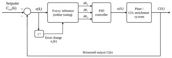
where K_p0, K_i0, and K_d0 are the same baseline gains used by the fixed-parameter PID controller. The updated K_p(k), K_i(k), and K_d(k) values were clipped to the ranges listed in Table A1 and constrained to remain nonnegative to prevent reversal of the control action. Conventional fuzzy PID retained the operating-point feedforward term, 0–100% output saturation, and conditional integration anti-windup rule of the fixed-parameter PID controller. Only the PID gains were updated online; the controller did not include the dynamic-target generator, integral attenuation, proportional soft dead zone, zero-crossing integral release, or per-step output-rate limit (Figure 5).

Figure 5. Online parameter-tuning architecture of conventional fuzzy PID.

2.2.3. DT-FPID Control

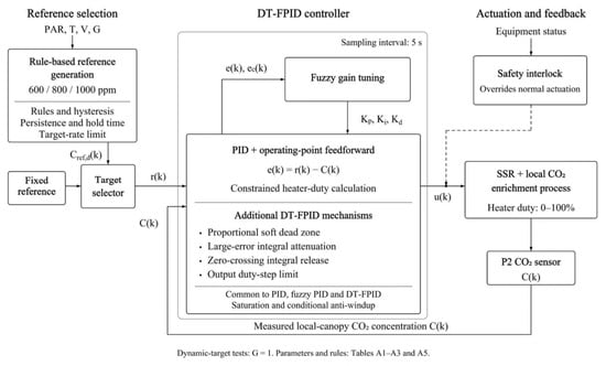
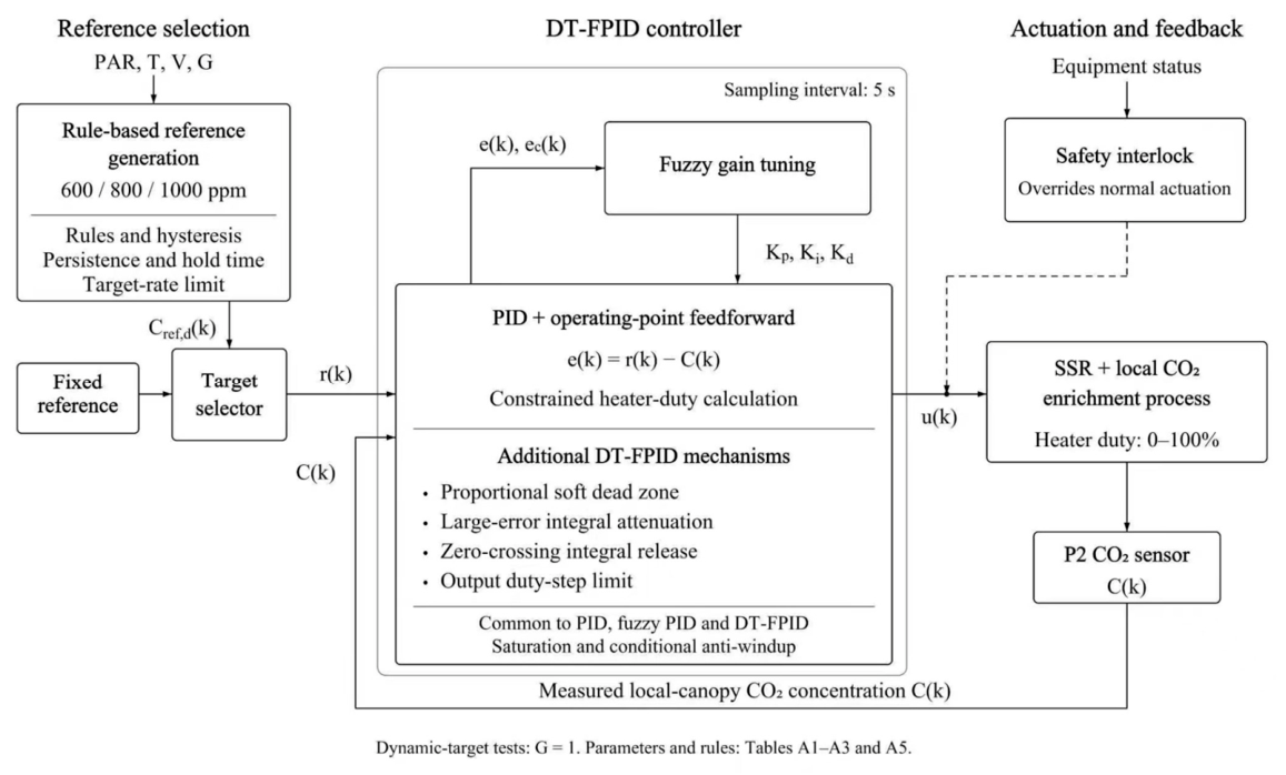
A dynamic-target generator and a constrained execution layer were added to conventional fuzzy PID to construct DT-FPID. All three methods used the same operating-point feedforward term, baseline gains, and conditional integration anti-windup rule. DT-FPID additionally incorporated a proportional soft dead zone, integral attenuation under large errors, zero-crossing integral release, and an output-rate constraint (Figure 6). Depending on the source of the reference, DT-FPID operated in fixed-setpoint or dynamic-setpoint mode. For fixed-target tracking and ventilation-disturbance tests, the dynamic-target generator was disabled and a preset target was applied directly to evaluate the combined effect of fuzzy gain tuning and the constrained execution layer. In the dynamic-target tests, a tiered-target generator based on predefined environmental thresholds was enabled to generate and track engineering reference values from environmental inputs. Here, “dynamic” means only that the reference value changes over time with the environmental inputs and rule state; it does not denote online learning, self-updating thresholds, or real-time optimization of physiologically or economically optimal crop targets.

Figure 6. Rule-based reference generation and constrained DT-FPID closed-loop control. The selected reference r(k) is either the fixed target C_ref(k) or the dynamic target C_ref,d(k); C(k) is the local canopy CO₂ concentration measured at P2, and u(k) is the heater duty command during normal operation. Fuzzy tuning updates the PID gains using e(k) = r(k) − C(k) and e_c(k) = e(k) − e(k − 1). The calculation block lists the additional DT-FPID mechanisms and the saturation and conditional anti-windup rules shared by the three compared controllers; the list does not denote program execution order. The safety interlock can override normal actuation. G is fixed at 1 in the dynamic-target tests. Parameters and rules are provided in Table A1, Table A2, Table A3 and Table A5. Discrete simulation settings and first-step consistency checks are provided in Supplementary Table S6.

The inputs to the dynamic-target generator were PAR(k), air temperature T(k), ventilation state V(k), and control level G(k). Values of V = 0, 1, and 2 represented no active ventilation, conventional natural ventilation, and intensified ventilation, respectively. G was an internal program variable with values 0, 1, and 2 denoting low, validation, and high control levels; G = 1 was preset for the five-leaf-stage dynamic-target experiments. G did not correspond to BBCH or any standard tomato phenological code and served only as an engineering input for candidate-target selection. It was not used to infer a physiologically optimal CO₂ concentration. Candidate targets were 600, 800, and 1000 ppm:

$$C_{\mathrm{c}\mathrm{a}\mathrm{n}\mathrm{d}}\left(k\right)=\left\{\begin{array}{ll}600,& V\left(k\right)=2orPAR\left(k\right)<400orT\left(k\right)<18orT\left(k\right)>34;\\ 1000,& PAR\left(k\right)\ge 700, 22\le T\left(k\right)\le 32, V\left(k\right)\le 1, G\left(k\right)\ge 1;\\ 800,& \mathrm{otherwise}.\end{array}\right.$$

(7)

Candidate conditions had to remain satisfied for 3 min, and consecutive switches were separated by at least 10 min. Hysteresis bands of ±50 μmol·m⁻²·s⁻¹ for PAR and ±1 °C for air temperature were used to suppress frequent switching when environmental variables fluctuated near their thresholds. The 600, 800, and 1000 ppm levels were used as engineering reference levels supported by published studies of tomato CO₂ responses [19]. PAR, temperature, and ventilation state were used to determine the direction of target adjustment, with light–CO₂ responses and ventilation conditions providing support for the rule direction [23]. The specific PAR and temperature boundaries were defined as engineering tiering thresholds for this study, and the basis for the anti-chattering execution parameters is provided in Table A5. Once the persistence, hold-time, and hysteresis conditions were satisfied, an accepted target C_acc(k) was obtained and then smoothed by a rate limiter to generate the dynamic reference:

$$C_{\mathrm{r}\mathrm{e}\mathrm{f},\mathrm{d}}\left(k\right)=C_{\mathrm{r}\mathrm{e}\mathrm{f},\mathrm{d}}\left(k-1\right)+sat\left[C_{\mathrm{a}\mathrm{c}\mathrm{c}}\left(k\right)-C_{\mathrm{r}\mathrm{e}\mathrm{f},\mathrm{d}}\left(k-1\right), -R\Delta t, R\Delta t\right]$$

(8)

where the maximum target rate R was 50 ppm·min⁻¹ and Δt was 5/60 min. This dynamic target was intended for staged engineering control and did not represent a physiologically optimal concentration.

The DT-FPID control errors were defined as follows:

$$e_{\mathrm{d}}\left(k\right)=C_{\mathrm{r}\mathrm{e}\mathrm{f},\mathrm{d}}\left(k\right)-C\left(k\right)$$

(9)

$$e_{c,d}\left(k\right)=e_{\mathrm{d}}\left(k\right)-e_{\mathrm{d}}\left(k-1\right)$$

(10)

Let r(k) denote the selected reference, namely C_ref(k) in fixed-target mode or C_ref,d(k) in dynamic-target mode. The unified control error and its per-sample increment were e(k) = r(k) − C(k) and e_c(k) = e(k) − e(k − 1), respectively; e_d(k) and e_c,d(k) in Equations (9) and (10) are the corresponding special case when r(k) = C_ref,d(k). These two signals were used for fuzzy gain tuning. The soft dead zone acted only on the proportional channel. In the integral channel, the stored integral state was released on an error sign change before the candidate integral state was formed using the current error and the applicable integral weight. The unconstrained control command combined operating-point feedforward, the proportional term, the candidate integral term, and the filtered measurement-derivative term. The applicable duty-step limit was then imposed, followed by saturation to 0–100%. The mechanism list in Figure 6 summarizes functional components rather than a separate sequential execution pipeline. The soft dead zone was defined as follows:

$$e_{\mathrm{z}}\left(k\right)=\left\{\begin{array}{ll}0,& \left|e_{\mathrm{d}}\left(k\right)\right|\le \delta ;\\ e_{\mathrm{d}}\left(k\right)-\delta sgn\left[e_{\mathrm{d}}\left(k\right)\right],& \left|e_{\mathrm{d}}\left(k\right)\right|>\delta .\end{array}\right.$$

(11)

where the soft-dead-zone width Δ was 8 ppm and was applied only to the proportional channel; the integral channel retained the original error. The integral weight was defined as follows:

$$\beta \left(k\right)=\left\{\begin{array}{ll}0.65,& \left|e_{\mathrm{d}}\left(k\right)\right|>e_{\mathrm{I}};\\ 1,& \left|e_{\mathrm{d}}\left(k\right)\right|\le e_{\mathrm{I}}.\end{array}\right.$$

(12)

The integral-attenuation threshold was 50 ppm. When the absolute error exceeded this threshold, the integral weight was 0.65; otherwise, it was 1. When the error changed sign between two successive samples, the stored integral state was first released to zero and Equation (13) then formed the current integral candidate. Whether that candidate was retained was determined by the conditional anti-windup rule in Section 2.2.1. Equation (14) defines the control command before output constraints.

$$I_{\mathrm{e}}\left(k\right)=I_{\mathrm{e}}\left(k-1\right)+\beta \left(k\right)e_{\mathrm{d}}\left(k\right)\Delta t$$

(13)

$${\mathrm{u}}^{*}\left(k\right)=u_b\left(k\right)+K_p\left(k\right)e_z\left(k\right)+K_i\left(k\right)I_e\left(k\right)-K_d\left(k\right)d_f\left(k\right)$$

(14)

The per-step output change and final amplitude were constrained as follows:

$$\Delta u_{\mathrm{c}}\left(k\right)=sat\left[{\mathrm{u}}^{*}\left(k\right)-u\left(k-1\right), -\Delta u_{max}, \Delta u_{max}\right]$$

(15)

$$u\left(k\right)=sat\left[u\left(k-1\right)+\Delta u_{\mathrm{c}}\left(k\right), 0, 100\right]$$

(16)

The maximum per-step output change was 30 percentage points. The 0–100% amplitude limit was applied after the duty-step limit, and the saved integral state was updated using the conditional rule in Section 2.2.1 when the final output reached either bound.

Figure 6 summarizes reference selection, fuzzy gain tuning, and constrained closed-loop control. At each 5 s control interval, the selected reference and the CO₂ concentration measured at P2 were used to update the control calculation. Fixed-target operation bypassed the dynamic-target generator, whereas dynamic-target operation updated the reference according to the prescribed rules. During normal operation, the controller command regulated the solid-state-relay heater duty; fault or over-limit conditions allowed the safety interlock to override normal actuation. The discrete calculation and state-update rules are specified by the equations and descriptions in this section.

2.3. Process Identification and Simulation

Before model development, the CM1106H-NS sensors at P0–P4 were placed in the same calibration environment and exposed to reference concentrations of 400, 600, 800, and 1000 ppm. Low-cost NDIR CO₂ sensors require comparison against a reference instrument and calibration to improve measurement consistency [24]. After each concentration stabilized, 90 observations were recorded and a separate linear correction relationship, C_i,corr = a_iC_i,raw + b_i, was established for each sensor. Specifications of the reference analyzer, the four-point calibration protocol, and the correction parameters are provided in Supplementary Table S2.

To characterize the steady-state relationship between heater input and gas release, the heater duty cycle was sequentially set to 20%, 40%, 60%, 80%, and 100%, while total outlet volumetric flow rate, CO₂ volume fraction, reactor temperature, P2 concentration, and pipeline pressure were measured simultaneously. CO₂-equivalent flow was calculated using Equation (17), where the first term is the total outlet volumetric flow and the second is the CO₂ volume fraction. Each level was maintained for 25 min and repeated three times, and the final 5 min mean represented the corresponding condition. Flowmeter model, range, accuracy, and temperature–pressure reference conditions are provided in Supplementary Table S2.

$$Q_{\mathrm{C}{\mathrm{O}}_2}=Q_{\mathrm{g}}{\phi }_{\mathrm{C}{\mathrm{O}}_2}$$

(17)

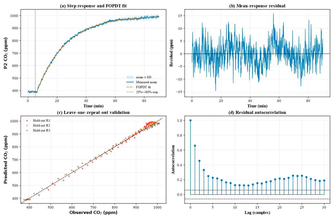
Step-response tests were conducted using the same apparatus under stable conditions. After P2 returned to 390 ± 5 ppm, the duty cycle was maintained at 20% and then increased to 80% at 5 min. Data were recorded continuously for 90 min, with three replicates. The operating-point duty cycle u₀ and concentration C₀ of the deviation model were 20% and 390.833 ppm, respectively.

An FOPDT model was used to describe the response of P2 concentration to changes in heater duty cycle. Bi et al. proposed a robust method for identifying FOPDT models from step responses [25]. Fedele developed a method for estimating first-order-plus-dead-time parameters from step-response data [26]. In this study, logarithmic parameterization and MATLAB fminsearch were used to minimize the residual sum of squares. The three replicate responses and the mean response were identified separately, and fitting quality and parameter stability were evaluated using R², RMSE, and leave-one-replicate-out validation. Initial parameter values and the computational procedure are provided in Supplementary Method S1. The model fitted to the mean response was subsequently used as a common low-order nominal plant for controller comparison and was not intended to replace the full dynamics of the actual Chinese solar greenhouse.

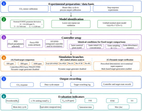
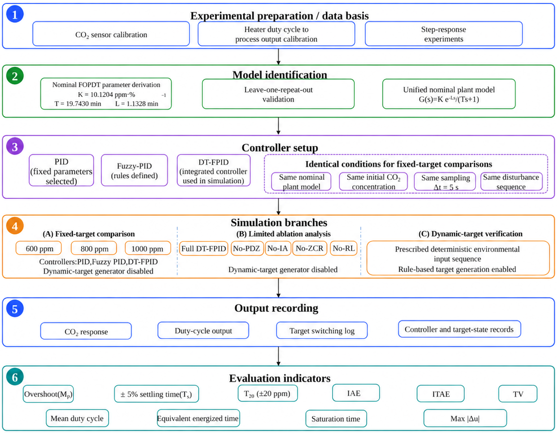
A unified discrete simulation was implemented in MATLAB R2024b (The MathWorks, Inc., Natick, MA, USA), including fixed-target controller comparison, limited DT-FPID ablation analysis, and dynamic-target validation. Fixed-target comparisons used the same FOPDT nominal process, initial state, sampling interval, external disturbance, and evaluation window; PID, conventional fuzzy PID, and DT-FPID differed only in control strategy, and the dynamic-target generator was disabled for all three. To evaluate the mechanisms added to DT-FPID relative to conventional fuzzy PID, single-module-removal ablations were conducted under the same simulation conditions by disabling the proportional soft dead zone, large-error integral attenuation, zero-crossing integral release, or per-step output-rate limit, respectively. Maximum overshoot, ±5% settling time, T₂₀, ITAE, total variation, and maximum single-step duty-cycle change (Max |Δu|) were compared. When the per-step output-rate limit was disabled, the 0–100% output-amplitude limit and the conditional anti-windup mechanism common to all three controllers were retained. The dynamic-target simulation used only the complete DT-FPID to test tiered-target generation, persistence checking, hysteresis, minimum hold time, target-rate limiting, and closed-loop tracking; it was not used to determine physiologically or economically optimal target concentrations (Figure 7). The ablation configurations and complete results are provided in Supplementary Table S3.

Figure 7. Simulation workflow of the DT-FPID control system.

The fixed-target comparison, limited ablation analysis, and dynamic-target simulation used common controller-step and plant-state update functions. The nominal-plant parameters were taken from the mean-response identification in Table 2, and the baseline controller and constraint settings are listed in Table A1. No controller- or target-specific retuning was performed for the complete-controller comparisons; each ablation configuration changed only the setting associated with the removed mechanism, while all other comparison conditions remained unchanged.

Table 2. FOPDT parameter identification and leave-one-replicate-out validation.

Type	Data Source/Combination	K (ppm·%−1)	T (min)	L (min)	R2	RMSE (ppm)
Parameter identification	Replicate 1	9.8441	18.3800	0.8459	0.998420	7.276
	Replicate 2	10.1131	19.7953	1.2251	0.998526	7.288
	Replicate 3	10.4256	21.1290	1.3237	0.998604	7.308
	Mean response	10.1204	19.7430	1.1328	0.999420	4.561
Leave-one-replicate-out validation	Model: replicates 2 and 3; validation: replicate 1	10.2676	20.4618	1.2704	0.993086	15.219
	Model: replicates 1 and 3; validation: replicate 2	10.1249	19.7274	1.0800	0.998390	7.617
	Model: replicates 1 and 2; validation: replicate 3	9.9751	19.0700	1.0403	0.994192	14.905

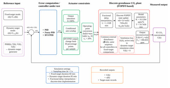
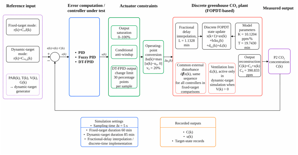
The discrete simulation structure is shown in Figure 8 and included environmental inputs, dynamic-target generation, fuzzy tuning, positional PID control, actuator constraints, the FOPDT process, and data recording. The nominal process was:

$$G\left(s\right)={\displaystyle \frac{10.1204e^{-1.1328 \mathrm{s}}}{19.7430 \mathrm{s}+1}}$$

(18)

Figure 8. Discrete simulation structure of the greenhouse CO₂ concentration-control system.

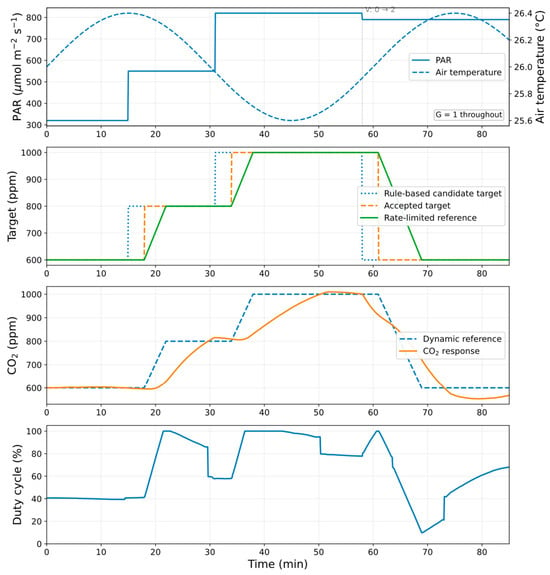
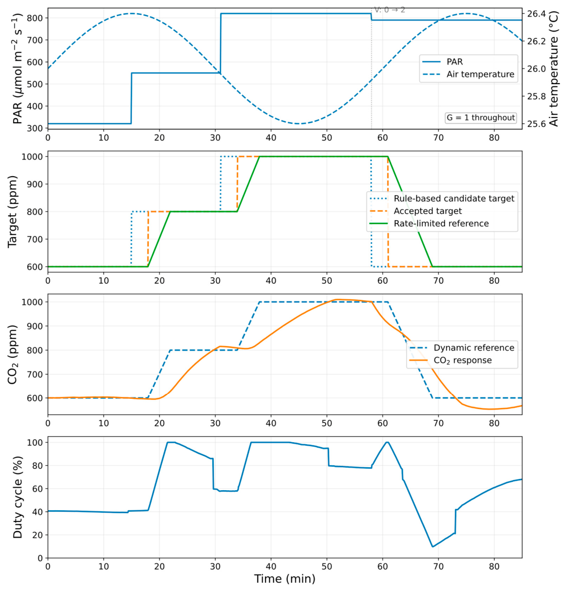
The continuous model was discretized at a 5 s sampling interval. The discrete coefficient and input gain were calculated using Equation (19), and the dead time was implemented by linear interpolation between adjacent samples. For fixed-target simulations, all three controllers at a given target concentration received the same external-disturbance sequence to ensure identical comparison conditions. The dynamic simulation used a prescribed deterministic environmental sequence: PAR was 320, 550, 820, and 790 μmol·m⁻²·s⁻¹ during 0–15, 15–31, 31–58, and >58 min, respectively; air temperature varied as 26 + 0.4 sin(2πt/60) °C; and at 58 min the ventilation state changed from V = 0 to V = 2, while G remained fixed at 1. The ventilation-loss term in Equation (20) was applied only in the dynamic-target simulation. Ventilation-loss coefficients for V = 0, 1, and 2 were 0, 0.015, and 0.060 min⁻¹, respectively. The complete recurrence is provided in Supplementary Method S1 and Table A1.

The effective incremental plant input was Δu(k) = max[u(k) − u₀, 0] and entered the state update after the dead-time block; thus, an actual duty below the operating point was not interpreted as negative incremental gas release. MATLAB twister used a base seed of 20260629. For every controller and ablation configuration at a fixed target, the seed was reset to the base seed plus the target concentration so that all configurations at that target received the same disturbance sequence; the dynamic-target branch used the base seed plus 9000. The dynamic environmental sequence was deterministic, whereas the process disturbance retained a stochastic component. In the discrete ventilation term, the loss acted only on concentration above the operating point, i.e., on the nonnegative part of C(k) − C₀ in Equation (20).

$$a=exp\left(-{\displaystyle \frac{\Delta t}{T}}\right), b=K\left(1-a\right)$$

(19)

d_V(k) = −γ_V max[C(k) − C₀, 0] Δt

(20)

The initial CO₂ concentration in the fixed-target simulations was 390.0 ppm, whereas the operating-point concentration C₀ of the FOPDT deviation model was 390.833 ppm. Fixed-target simulations tracked 600, 800, and 1000 ppm over 60 min. The performance indices included maximum overshoot, ±5% operational settling time, ±20 ppm settling time (T₂₀), steady-state error, IAE, ITAE, and actuator metrics; both settling-time criteria required continuous residence within the corresponding band for 5 min. T₂₀ characterized convergence near the target and did not imply an absolute sensor accuracy of 20 ppm. Dynamic-target indices included the number of target switches, the number of unintended switches, the maximum target-change rate, the maximum transition error, and dynamic IAE. The same tracking-index definitions were used for fixed-target simulation and greenhouse fixed-target experiments. IAE and ITAE were calculated using Equations (21) and (22).

In the fixed-target simulations, the initial integral and filtered-derivative states were zero, the previous applied output was initialized to 20%, and the input-delay history was initialized at that operating point. The dynamic-target simulation started at 600 ppm, and its delay history was initialized at the operating-point feedforward duty corresponding to 600 ppm. The complete initialization, control-step order, disturbance settings, and equation-based first-step consistency checks are provided in Supplementary Method S1 and Supplementary Table S6.

2.4. Greenhouse Experiments

2.4.1. Experimental Conditions

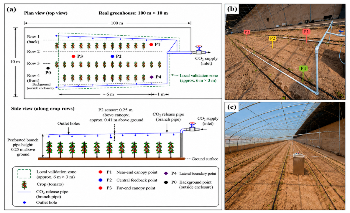
The experiments were conducted from 1 to 21 May 2026 in a 100 m × 10 m × 6.0 m Chinese solar greenhouse planted with tomato in a yellow-sand substrate at the Sixth Regiment, First Division of the Xinjiang Production and Construction Corps, Alar City, China. Previous research has shown that Chinese solar greenhouse structures in Xinjiang desert regions differ in temperature–humidity conditions and thermal-insulation performance [27]. Fixed-target tracking, short-term ventilation-disturbance, and dynamic-target tests were all conducted within a 6 m × 3 m local validation zone. The experimental system comprised the prototype CO₂ enrichment unit, near-canopy delivery pipelines, measurement points P0–P4, a PLC, and a data-logging terminal. An axial-flow fan was additionally used for the short-term ventilation-disturbance tests. The equipment and measurement-point layout are shown in Figure 9.

Figure 9. Experimental layout of the local validation zone in the 100 m × 10 m Chinese solar greenhouse. (a) Plan-view layout and side-view schematic of the local validation zone; (b) field photograph showing the CO₂ supply pipeline and measurement points P1–P4; (c) interior photograph of the experimental Chinese solar greenhouse and local validation zone.

The tomato cultivar “Jingfan 401” was grown in the validation zone and was at the five-leaf stage during the experiments, with a mean plant height of 16.2 ± 1.4 cm. Sixty plants were arranged in four rows, with row and plant spacings of 0.4 and 0.38 m, respectively. Two perforated branch pipes, each 12 mm in internal diameter and 6.0 m long, were installed along the crop rows. Outlet holes were 2.0 mm in diameter and spaced 0.3 m apart, and each branch pipe served two rows. The perforated pipes were installed 0.25 m above the ground. P2 was positioned 0.25 m above the canopy, corresponding to approximately 0.41 m above the ground based on mean plant height. P2 was located at the center of the validation zone and served as the sole closed-loop feedback point. P1, P3, and P4 were located near the supply end, at the far end, and at the lateral boundary, respectively, and were used to evaluate the local canopy CO₂ distribution. P0 was outside the enrichment zone and measured the greenhouse background concentration. P0, P1, P3, and P4 were not used for controller feedback.

At the start of the 27 fixed-target runs, the P2 concentration and initial ammonium bicarbonate mass in the reactor were 389.02 ± 4.55 ppm and 1.501 ± 0.028 kg, respectively. Mean PAR, air temperature, and relative humidity during these runs were 728.49 ± 65.54 μmol·m⁻²·s⁻¹, 25.12 ± 0.26 °C, and 60.94% ± 0.19%, respectively. No active ventilation was applied during fixed-target tests, and the ventilation state remained V = 0. Ventilation conditions for the dynamic-target and short-term ventilation-disturbance experiments are described in Section 2.4.2 and Section 2.4.3, respectively. These data were summarized across individual runs as mean ± standard deviation.

2.4.2. Target-Concentration Tracking Experiments

Fixed targets were set at 600, 800, and 1000 ppm and tested using PID, conventional fuzzy PID, and DT-FPID. Three independent runs were conducted for each controller–target combination, giving 27 fixed-target tests in total. The three runs for each combination were completed on different dates. Under each target, the three control methods were rotated among the 09:00, 11:30, and 14:00 experimental time slots to reduce systematic bias associated with a fixed running order; the experiments were not formally randomized. The date, time slot, and concurrent conditions of each run are provided in Supplementary Table S1. Before and after each test, ventilation was used to return P2 to the background concentration. P2 concentration, duty cycle, and environmental and equipment-process variables were recorded continuously.

To ensure comparability among the 57 fixed-target, disturbance-recovery, and dynamic-target runs, the reactor charge and scrubbing solution were restored to prescribed conditions before each run, the gas line was purged, and P2 was returned to background concentration. Reactor temperature, pipeline pressure, liquid level, valves, the solid-state relay, and sensor communications were also checked. Before each run, P2 concentration, PAR, air temperature and humidity, ventilation state, reactor temperature, initial material mass, and scrubbing-solution condition were recorded. The complete run order and state-restoration records are provided in Supplementary Table S1.

All fixed-target tests used a 5 s sampling interval, a 0–100% output range, and a 0–60 min evaluation window. From 19 to 21 May 2026, three independent dynamic-target field tests were conducted using the same predefined composite scenario structure, with DT-FPID used in all three runs. Each run began from a stable 600 ppm condition and continuously used the measured PAR, air temperature, and ventilation state from that run, while the internal control level was fixed at G = 1. Candidate targets, accepted targets, rate-limited targets, P2 concentration, and duty cycle were recorded simultaneously, and the target sequence, number of switches, number of unintended switches, maximum target rate, maximum transition error, and dynamic IAE were evaluated.

The fixed-target indices comprised maximum overshoot, ±5% operational settling time, ±20 ppm settling time (T₂₀), steady-state error, IAE, and ITAE. The two settling times were defined as the times required for P2 concentration to first enter and then remain for 5 min within ±5% of the target and within ±20 ppm of the target, respectively. Steady-state error was defined as the difference between the final 5 min mean concentration and the target. IAE and ITAE were calculated using Equations (21) and (22).

$$\mathrm{I}\mathrm{A}\mathrm{E}={\displaystyle \sum _{k=1}^N}\left|C_{\mathrm{r}\mathrm{e}\mathrm{f}}-C\left(k\right)\right|\Delta t$$

(21)

$$\mathrm{I}\mathrm{T}\mathrm{A}\mathrm{E}={\displaystyle \sum _{k=1}^N}{t}_{\mathrm{k}}\left|C_{\mathrm{r}\mathrm{e}\mathrm{f}}-C\left(k\right)\right|\Delta t$$

(22)

where N is the number of samples in the 0–60 min evaluation window and the sampling interval Δt was 5/60 min. All indices were calculated from unsmoothed 5 s raw data; a three-point moving average was used only for plotting. Steady-state error and T₂₀ described control performance within the evaluation window and were not equivalent to the absolute accuracy of a single sensor measurement.

Simultaneous P0–P4 monitoring was conducted as a separate local spatial-distribution experiment using DT-FPID, with target concentrations of 600, 800, and 1000 ppm and three independent runs at each target, giving nine runs in total. This experiment was used only to characterize CO₂ spatial gradients within the local validation zone and was not included in the 57 formal controller-performance evaluation runs. For the auxiliary measurement points, the final 5 min after P2 had entered and remained within ±5% of the target for 5 min was used as the common evaluation window. The stable-window mean was first calculated for each run and then summarized as mean ± standard deviation. Deviations of P1, P3, and P4 relative to P2 were calculated using Equation (23), while P0 served only as the background point.

$$D_{\mathrm{i}}={\displaystyle \frac{C_{\mathrm{i}}-C_{\mathrm{P}2}}{C_{\mathrm{P}2}}}\times 100\%$$

(23)

2.4.3. Ventilation-Disturbance Recovery Experiments

Fixed-target tracking and disturbance-recovery experiments were conducted independently and did not share data from the same run. The disturbance tests likewise comprised three target concentrations, three control methods, and three replicates, for a total of 27 runs. The system was first operated at the assigned target and control method. When P2 entered and remained within ±5% of the target for 5 min, that instant was defined as the start of the disturbance-stage time axis. The system then operated steadily for 10 min, after which the same axial-flow fan delivered local ventilation at 1.7 m³·min⁻¹ from 10 to 13 min for 180 s. Recording continued to 40 min. Time in the disturbance-response plots and the associated indices was referenced to the start of the disturbance stage.

Maximum recovery deviation was the largest absolute deviation of P2 from the target after the disturbance. Recovery time was the time required after the disturbance ended for P2 to re-enter and remain within ±5% of the target for 5 min. Post-recovery bias was the difference between the 35–40 min mean concentration and the target. IAE and ITAE were calculated over 10–40 min, with the disturbance onset used as the time origin for ITAE. The 27 fixed-target runs, 27 ventilation-disturbance runs, and 3 dynamic-target runs together constituted the 57 field runs used for formal controller-performance evaluation. For the fixed-target and ventilation-disturbance tests, one complete independent run was the statistical unit. The 5 s continuous samples were used only to calculate the time-series performance metrics for that run and were not treated as additional independent replicates. Each treatment combination was reported as mean ± standard deviation from three independent runs, whereas the three dynamic-target runs were reported individually. All completed runs were included in the analysis; no run was excluded because of missing values, communication faults, or interlock alarms. Because each treatment combination comprised only three independent runs, the analysis was descriptive and no inferential significance testing was performed.

3. Results

3.1. CO₂ Enrichment System Characterization and Control Simulation

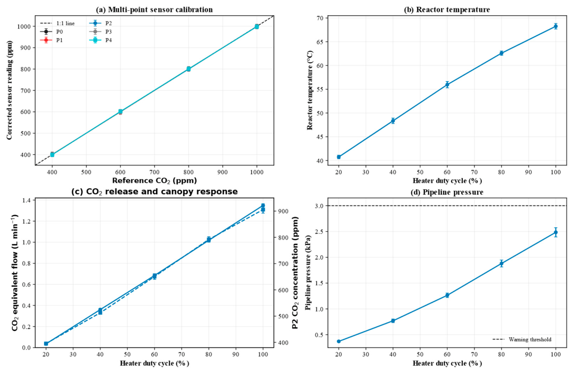
Sensor calibration and gas-release characterization are shown in Figure 10. After linear correction, the P0–P4 sensors yielded R² values of 0.99757–0.99876 and RMSE values of 7.86–11.02 ppm; corrected values were used in all subsequent analyses. As heater duty cycle increased from 20% to 100%, mean reactor temperature increased from 40.74 to 68.26 °C, CO₂-equivalent flow from 0.039 to 1.309 L·min⁻¹, mean P2 concentration from 394.29 to 921.59 ppm, and pipeline pressure from 0.371 to 2.485 kPa, which remained below the 3.0 kPa warning threshold. These results indicate that heater duty cycle continuously regulated gas-release intensity and provided a stable manipulated input for process identification.

Figure 10. CO₂ sensor calibration and gas-release characterization at different heater duty cycles.

At heater duty cycles of 40–100%, the apparent NH₃ removal between the upstream and downstream scrubber measurements was 89.6–94.7% across three replicates. The sensor reading at P2 ranged from 0.34 to 1.20 ppm, but these values were below the reliable quantification range of the safety-verification instrument. They were therefore treated only as low-level screening signals and were not used to assess long-term exposure or operational safety.

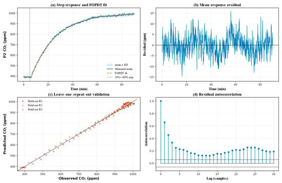
Step responses and FOPDT fits are presented in Figure 11 and Table 2. Across the three replicates, the static gain K, time constant T, and dead time L ranged from 9.8441 to 10.4256 ppm·%⁻¹, 18.3800 to 21.1290 min, and 0.8459 to 1.3237 min, respectively. The mean-response model yielded R² = 0.99942 and RMSE = 4.561 ppm. Leave-one-replicate-out validation produced R² values of 0.99309–0.99839 and RMSE values of 7.617–15.219 ppm, indicating that the low-order model approximated the dominant dynamics of the mean step response. However, residual autocorrelation exceeded the 95% confidence bounds at several lags, showing that the model did not fully capture higher-order dynamics arising from gas release, local mixing, and external disturbances. Accordingly, the model was used only as a nominal process for uniform controller comparisons.

Figure 11. Step response of the CO₂ process and FOPDT model fitting results.

The fixed-target comparisons, limited ablation analysis, and dynamic-target simulation reported below used the common implementation and parameter settings described in Section 2.3 and Supplementary Method S1. The implementation settings and analytical first-step consistency checks are summarized in Supplementary Table S6.

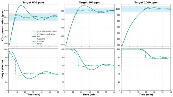
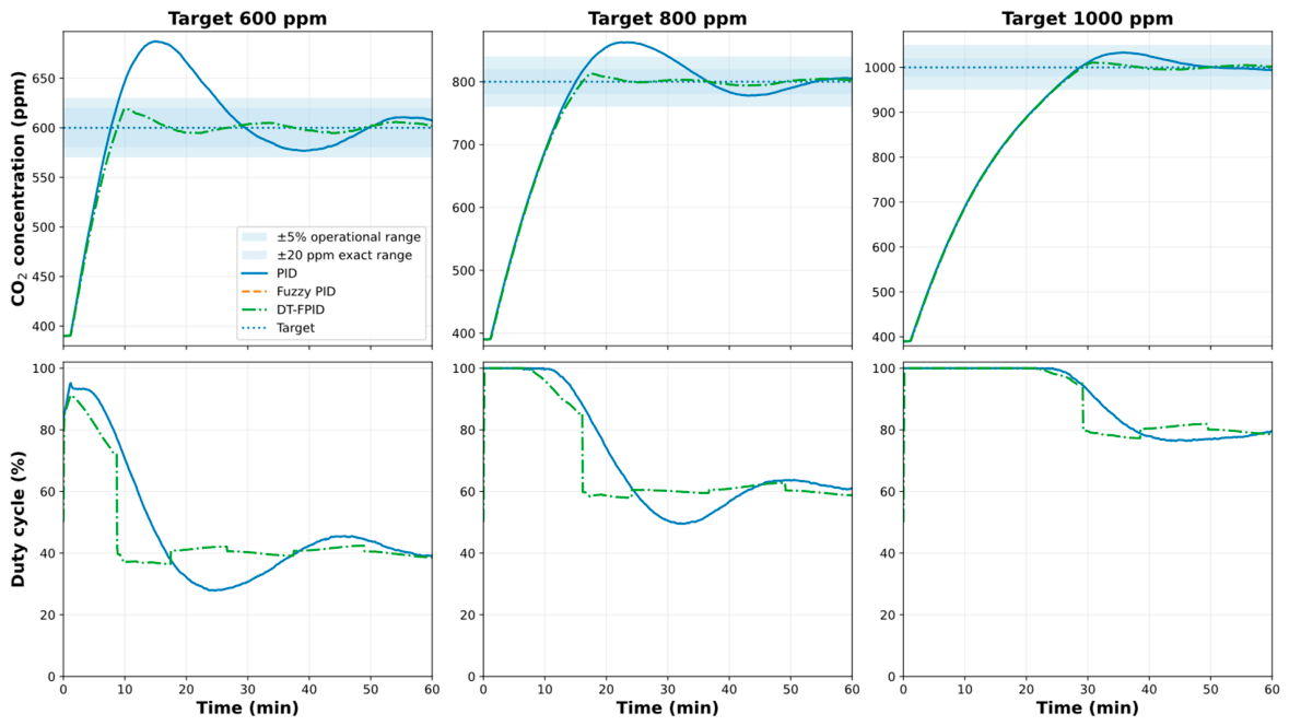
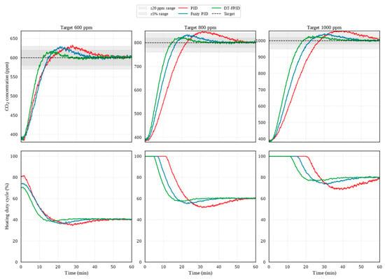
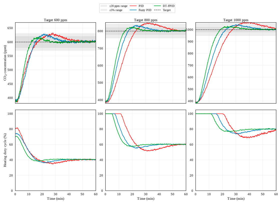
Fixed-target simulation results are shown in Figure 12 and Table 3. Across the three targets, DT-FPID yielded the lowest maximum overshoot and T₂₀. At 600 ppm, the ±5% operational settling time of DT-FPID was 7.25 min, substantially shorter than the 24.83 and 24.00 min obtained with PID and conventional fuzzy PID, respectively. At 800 and 1000 ppm, the corresponding DT-FPID settling times were 13.42 and 24.58 min and were broadly comparable to those of the two benchmark controllers. Compared with fixed-parameter PID, conventional fuzzy PID generally produced only modest improvements in maximum overshoot, IAE, and T₂₀. Saturation time and near-target convergence time generally increased with target concentration for all three controllers.

Figure 12. Simulated concentration responses, control outputs, and dual settling bands for PID, conventional fuzzy PID, and DT-FPID under fixed targets.

Table 3. Simulated performance indices of the three control methods under fixed targets.

Target (ppm)	Control Method	Maximum Overshoot (ppm)	±5% Operational Settling Time (min)	T20 (min)	IAE (ppm·min)	ITAE (ppm·min2)
600	PID	87.15	24.83	26.17	2403.8	37,686.7
	Fuzzy PID	87.07	24.00	25.33	2334.7	36,026.8
	DT-FPID	19.35	7.25	7.75	1190.3	9270.8
800	PID	62.82	13.00	33.33	4066.6	46,713.9
	Fuzzy PID	57.53	13.00	32.83	3972.9	44,132.2
	DT-FPID	13.32	13.42	14.75	3169.9	19,975.1
1000	PID	33.00	24.50	41.67	7586.1	75,718.5
	Fuzzy PID	31.24	24.50	40.83	7546.8	74,059.1
	DT-FPID	10.47	24.58	27.17	7348.1	65,650.7

Note: Both the ±5% operational settling time and T₂₀ (±20 ppm settling time) required continuous residence within the corresponding band for at least 5 min. Complete steady-state error and actuator metrics are provided in Supplementary Table S3.

Based on the fixed-target simulation results, relative to PID, DT-FPID showed approximately 68–79% lower maximum overshoot, approximately 35–70% shorter T₂₀, and approximately 13–75% lower ITAE across 600, 800, and 1000 ppm. At 600 ppm, the ±5% operational settling time was approximately 71% shorter, whereas at 800 and 1000 ppm it was broadly comparable to PID. Relative to conventional fuzzy PID, DT-FPID showed approximately 66–78% lower maximum overshoot and approximately 33–69% shorter T₂₀; the ±5% operational settling time was approximately 70% shorter at 600 ppm and broadly comparable at 800 and 1000 ppm. Actuator metrics showed that the mean duty cycle of DT-FPID was close to that of PID, whereas cumulative total output variation did not decrease consistently in simulation, indicating that the main advantages were overshoot suppression and convergence near the target rather than a uniform improvement in all actuator-activity metrics (Supplementary Table S3).

The limited ablation results are presented in Supplementary Table S3. Relative to full DT-FPID, removing zero-crossing integral release increased maximum overshoot across the three targets from 10.47–19.35 ppm to 34.05–69.05 ppm and prolonged T₂₀ from 7.75–27.17 min to 30.58–42.25 min. Removing large-error integral attenuation increased maximum overshoot, whereas the ±5% settling time did not deteriorate correspondingly. Removing the proportional soft dead zone increased total output variation at all three targets, while changes in the tracking-error metrics were smaller and not fully consistent in direction. Removing the per-step output-rate limit increased the maximum single-step duty-cycle change from 30 percentage points to 63.96–80.00 percentage points, while cumulative total variation decreased.

The dynamic-target simulation completed three prescribed target switches among the 600, 800, and 1000 ppm target levels, with zero unintended switches, a maximum target rate of 50.0 ppm·min⁻¹, a maximum transition-tracking error of 171.4 ppm, and a dynamic IAE of 3710.7 ppm·min (Figure 13). Execution of the prescribed target sequence showed that the complete target-generation logic operated according to the predefined rules under the environmental sequence and threshold combination used in this study. This result was not used to evaluate the physiological or economic optimality of the target concentrations.

Figure 13. Rule-based tiered-target generation, CO₂ tracking, and control output under the prescribed deterministic environmental input sequence.

3.2. Greenhouse Target-Tracking Performance

Fixed-target simulations and greenhouse experiments showed consistent trends in maximum-overshoot suppression and convergence near the target, although the degree of improvement in ±5% operational settling time was not fully consistent (Figure 14 and Table 4). Across all three targets, PID showed larger overshoot and a longer settling tail, conventional fuzzy PID provided some improvement, and DT-FPID produced a generally smoother response.

Figure 14. Fixed-target tracking responses in the Chinese solar greenhouse (mean ± SD, n = 3).

Table 4. Fixed-target tracking performance in the Chinese solar greenhouse.

Target (ppm)	Control Method	Maximum Overshoot (ppm)	Settling Time (min)	Steady-State Error (ppm)	IAE (ppm·min)	ITAE (ppm·min2)
600	PID	47.1 ± 2.3	15.1 ± 0.7	2.5 ± 3.0	2367.7 ± 792.9	27,311.6 ± 11,324.3
	Fuzzy PID	33.9 ± 3.1	12.4 ± 1.0	2.5 ± 0.9	2133.9 ± 170.1	20,033.3 ± 2425.7
	DT-FPID	24.0 ± 0.9	9.6 ± 0.9	0.9 ± 1.2	1565.1 ± 117.3	11,684.5 ± 920.6
800	PID	51.8 ± 2.0	19.8 ± 0.8	1.6 ± 0.8	5768.3 ± 159.3	65,365.3 ± 2710.6
	Fuzzy PID	40.3 ± 3.1	14.5 ± 1.4	1.8 ± 1.4	4083.7 ± 273.8	33,136.2 ± 4151.6
	DT-FPID	27.1 ± 3.4	11.9 ± 0.3	1.8 ± 0.7	3208.1 ± 37.4	21,150.5 ± 491.4
1000	PID	66.7 ± 3.1	24.1 ± 0.8	14.2 ± 6.4	9831.1 ± 393.2	124,234.6 ± 9762.5
	Fuzzy PID	49.9 ± 4.0	19.2 ± 0.8	1.1 ± 1.4	7473.5 ± 362.2	68,839.6 ± 5937.2
	DT-FPID	35.1 ± 3.5	15.5 ± 1.2	1.9 ± 1.0	5870.8 ± 360.4	42,885.7 ± 5755.3

Note: Values are means ± standard deviations of three independent runs (n = 3). Settling time was defined as the time required for the P2 concentration to first enter and remain within ±5% of the target for at least 5 min. Steady-state error was defined as the difference between the mean concentration during the final 5 min and the target. The comparisons are descriptive; no inferential significance tests were performed. Percentage differences reported in the text represent descriptive differences between group means. Single-run T₂₀ results are provided in Supplementary Table S5.

Based on descriptive comparison of group means from three independent runs, relative to PID, DT-FPID showed approximately 47–49% lower mean maximum overshoot, approximately 36–40% shorter mean ±5% settling time, and approximately 57–68% lower mean ITAE at 600, 800, and 1000 ppm. Relative to conventional fuzzy PID, the corresponding mean values were approximately 29–33%, 18–23%, and 36–42% lower, respectively. At 1000 ppm, the final 5 min steady-state errors of PID and DT-FPID were 14.2 ± 6.4 and 1.9 ± 1.0 ppm, respectively; this metric represents the mean over the stable window and not absolute sensor accuracy. Across all three targets, the mean duty cycle of DT-FPID was comparable to or slightly lower than that of PID, while mean total output variation was approximately 61–68% lower (Supplementary Table S3).

Results of the independent local spatial-distribution experiment are provided in Table A4. P1 concentrations were 3.04–3.48% higher than P2, whereas P3 and P4 were 4.17–4.66% and 7.30–8.03% lower, respectively. This gradient indicates that P2 represented the feedback state at the center of the local validation zone but not the CO₂ distribution throughout the entire greenhouse.

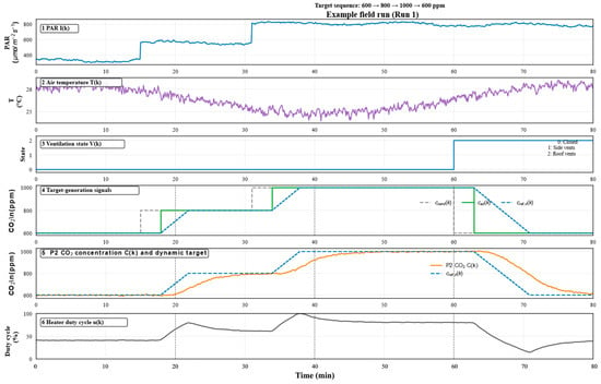
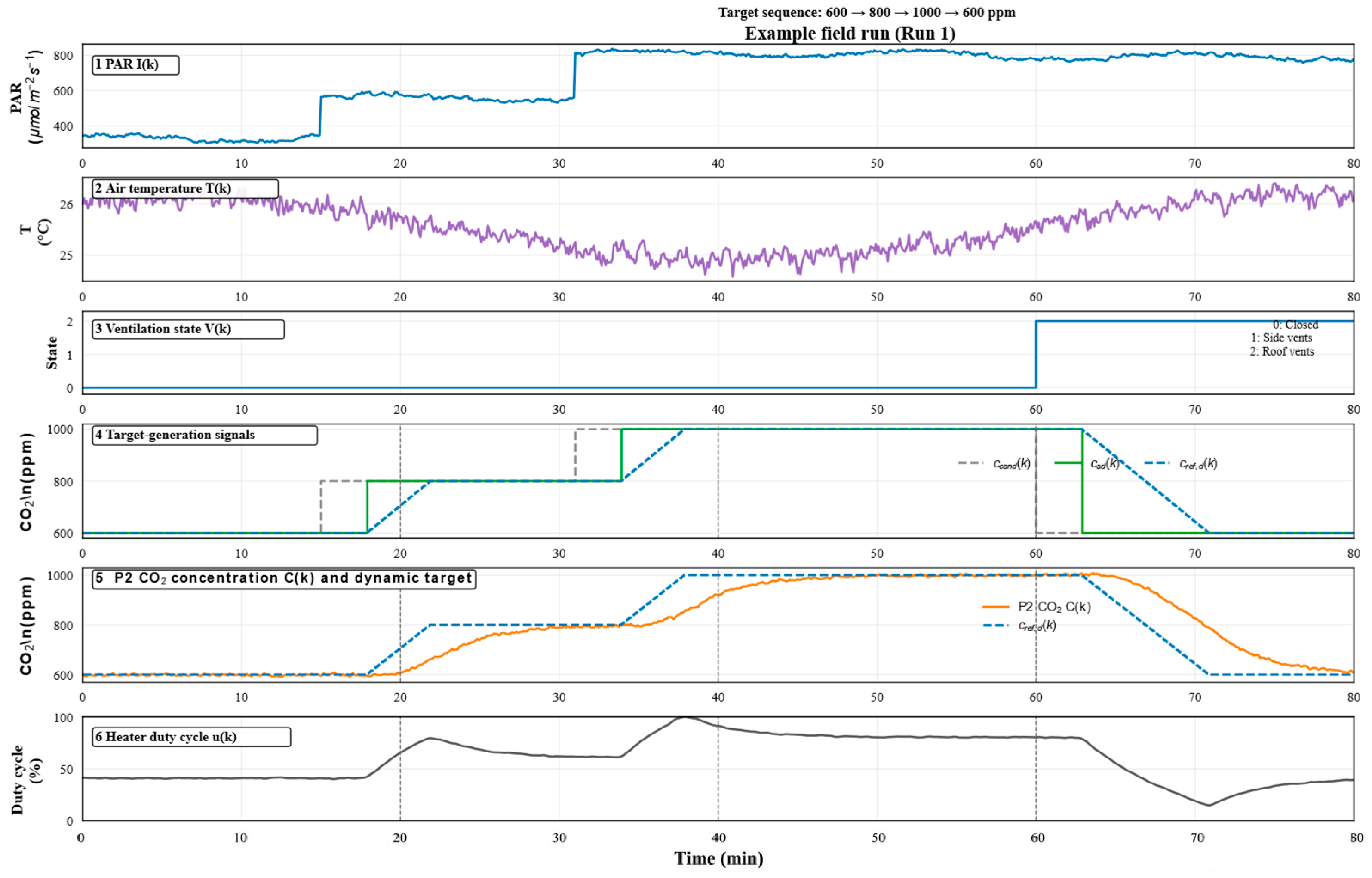
All three dynamic-target field experiments completed the three prescribed switches among the 600, 800, and 1000 ppm target levels, with zero unintended switches and a maximum target rate of 50.0 ppm·min⁻¹ in every run. The maximum transition-tracking error ranged from 186.2 to 193.3 ppm, the dynamic IAE ranged from 3224.2 to 3398.7 ppm·min, and the mean duty cycle was 58.9%. The three independent runs used the same predefined composite scenario structure and produced the same tiered-target switching process under the measured environmental inputs of each run, indicating repeatable execution of the rule under the conditions of this study. The example time series for Run 1 is shown in Figure 15, and the complete metrics and target-switching states for all three independent runs are provided in Supplementary Table S4.

Figure 15. Environmental inputs, rule-based target generation, P2 CO₂ tracking, and heating duty cycle for an example dynamic-target field run (Run 1) under the predefined composite scenario structure.

3.3. Greenhouse Recovery from Ventilation Disturbances

Based on the mean responses of three independent runs, PID showed larger concentration decreases and longer recovery times, conventional fuzzy PID was intermediate, and DT-FPID showed smaller mean recovery deviations and shorter mean recovery times (Figure 16 and Table 5). Based on descriptive calculations from group means, relative to PID, DT-FPID showed approximately 37–41% lower mean maximum recovery deviation, approximately 77–80% shorter mean recovery time, and approximately 73–75% lower mean ITAE across the three targets. Relative to conventional fuzzy PID, the corresponding mean values were approximately 21–26%, 48–58%, and 43–50% lower, respectively; the post-recovery bias was also numerically lower.

Table 5. Recovery performance following short-term ventilation disturbances in the Chinese solar greenhouse.

Target (ppm)	Control Method	Maximum Recovery Deviation (ppm)	Recovery Time (min)	Post-Recovery Bias (ppm)	IAE (ppm·min)	ITAE (ppm·min2)
600	PID	90.6 ± 5.0	17.0 ± 1.5	−17.8 ± 2.4	1134.4 ± 62.9	12,887.4 ± 1109.0
	Fuzzy PID	72.0 ± 2.9	8.1 ± 0.8	−5.6 ± 1.3	670.4 ± 43.9	6418.6 ± 674.5
	DT-FPID	57.2 ± 4.6	3.4 ± 1.3	−2.3 ± 1.1	387.7 ± 47.2	3218.1 ± 569.9
800	PID	124.2 ± 4.9	17.8 ± 1.3	−25.7 ± 1.4	1617.5 ± 39.7	18,635.5 ± 506.1
	Fuzzy PID	101.2 ± 6.3	8.8 ± 1.1	−11.2 ± 0.4	1005.9 ± 21.8	10,030.1 ± 110.1
	DT-FPID	75.3 ± 5.1	3.9 ± 1.0	−4.9 ± 0.5	594.3 ± 39.8	5117.3 ± 264.8
1000	PID	163.1 ± 2.1	17.9 ± 0.7	−35.7 ± 0.1	2158.6 ± 24.9	25,112.6 ± 235.5
	Fuzzy PID	126.1 ± 1.0	8.0 ± 0.8	−10.2 ± 0.5	1200.7 ± 46.1	11,312.9 ± 495.4
	DT-FPID	97.0 ± 4.0	4.2 ± 0.2	−5.6 ± 1.1	755.5 ± 47.2	6506.6 ± 472.2

Note: Values are means ± standard deviations of three independent runs (n = 3). Maximum recovery deviation was defined as the largest absolute deviation of the P2 concentration from the target after the ventilation disturbance. Recovery time was defined as the time required after the disturbance ended for the P2 concentration to re-enter and remain within ±5% of the target for at least 5 min. Post-recovery bias was defined as the difference between the mean concentration from t = 35 to 40 min and the target. IAE and ITAE were calculated over t = 10–40 min, with disturbance onset used as the time origin for ITAE. The comparisons are descriptive; no inferential significance tests were performed. Percentage differences reported in the text represent descriptive differences between group means.

Figure 16. CO₂ recovery response and heating duty-cycle output following short-term ventilation disturbance in the Chinese solar greenhouse (mean ± SD, n = 3; the shaded area indicates the 10–13 min ventilation-disturbance period).

Figure 16. CO₂ recovery response and heating duty-cycle output following short-term ventilation disturbance in the Chinese solar greenhouse (mean ± SD, n = 3; the shaded area indicates the 10–13 min ventilation-disturbance period).

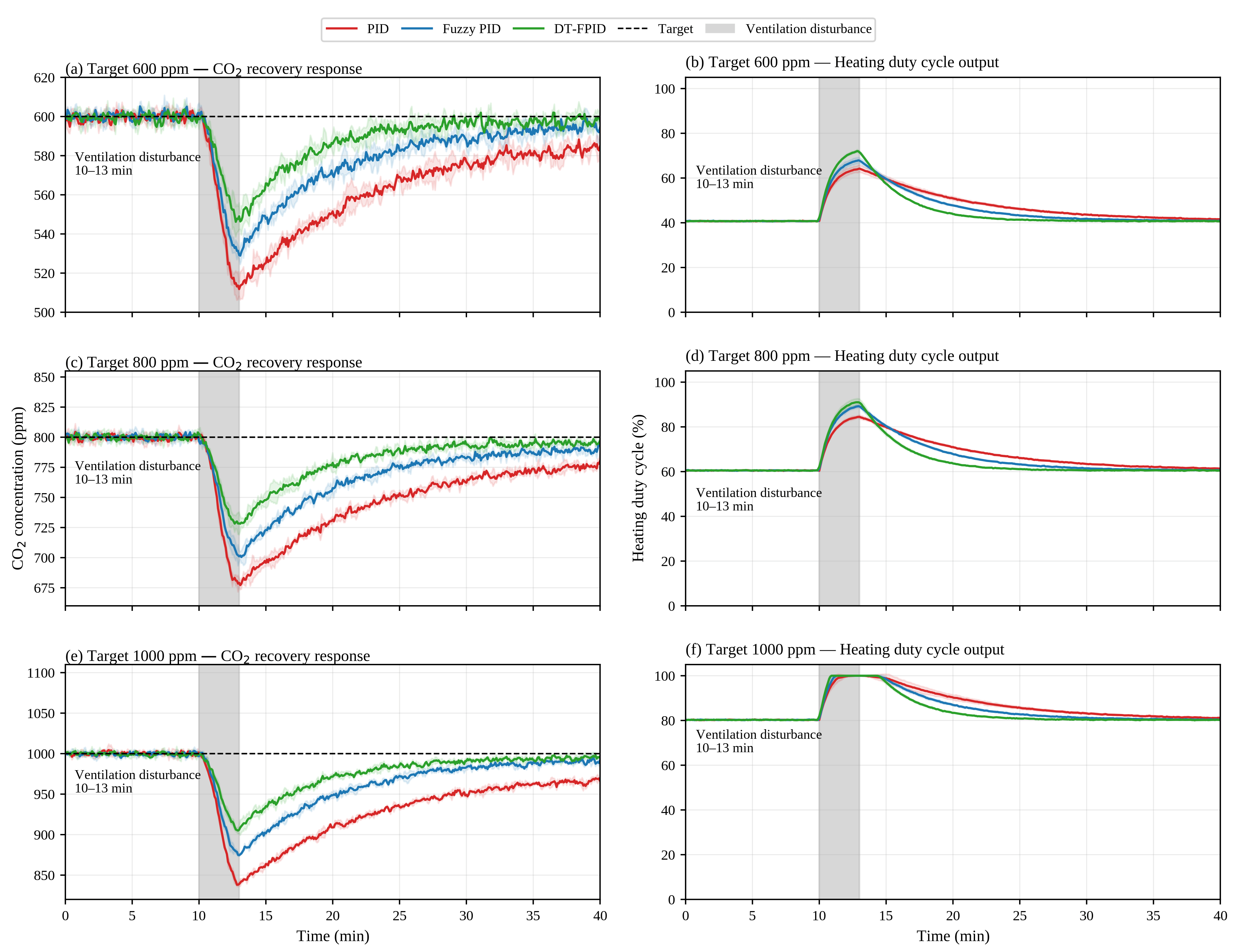
Across the three targets, the mean DT-FPID duty cycle was 3.4–4.9% lower than that of PID, whereas total output variation increased by 9.1–30.2% (Supplementary Table S3). Thus, faster disturbance recovery did not result from persistently higher heating output but was accompanied by more frequent or larger short-term adjustments during recovery.

4. Discussion

4.1. DT-FPID Control Performance and Mechanisms

Overall, fixed-target simulations and greenhouse experiments showed that DT-FPID mainly improved maximum overshoot and convergence near the target, whereas the ±5% settling times at 800 and 1000 ppm in simulation were broadly comparable to those of the control methods. Previous studies have shown that fuzzy PID can improve adaptability in greenhouse microclimate regulation [28]. PID–fuzzy combined control based on an EC model can also shorten settling time and reduce overshoot [29]. Predictive fuzzy PID can improve greenhouse environmental regulation through predictive compensation and online parameter tuning [13]. NMPC can use a dynamic model to handle multivariable coupling and actuator constraints [12]. Multilayer setpoint optimization further addresses the trade-off between energy consumption and crop production [30]. Unlike these approaches, the DT-FPID developed here does not perform multistep prediction or receding-horizon optimization and is intended primarily for PLC-based closed-loop execution of local canopy CO₂ targets; consequently, superiority should not be inferred from single performance metrics reported under different study conditions.

DT-FPID coordinates large-error response, convergence near the target, and actuator constraints through integral attenuation, a proportional soft dead zone, zero-crossing integral release, and an output-rate limit. In the fixed-target experiments, its mean duty cycle did not increase persistently, whereas mean maximum overshoot and total output variation were lower than with PID; during ventilation disturbances, faster recovery was accompanied by greater total output variation, indicating a trade-off between control speed and actuator activity. The limited ablation results (Supplementary Table S3) further show that removing zero-crossing integral release increased maximum overshoot to 34.05–69.05 ppm and prolonged T₂₀ to 30.58–42.25 min, making it the mechanism with the most pronounced effect on overshoot and convergence near the target. Removing large-error integral attenuation mainly increased maximum overshoot, whereas removing the proportional soft dead zone mainly increased total output variation near the target. Removing the per-step output-rate limit increased the maximum single-step duty-cycle change to 63.96–80.00 percentage points. Because these mechanisms operate within the same closed loop and interact with one another, the ablation results are interpreted only as performance changes after removal of a single mechanism and are not used for strictly independent or additive causal attribution.

The magnitude of improvement in simulation and field experiments was not fully consistent, mainly because the FOPDT nominal model describes only the dominant inertia and dead time, whereas field operation is additionally affected by crop uptake, structural leakage, local mixing, and ventilation changes. Natural ventilation alters air exchange between the greenhouse interior and exterior and the associated control load [31]. Chinese solar greenhouses exhibit pronounced spatiotemporal microclimate variation under natural ventilation [32]. Multipoint monitoring has shown that temperature, humidity, and CO₂ can form spatial gradients [33]. Naturally ventilated tomato greenhouses also exhibit vertical microclimate heterogeneity [34]. Accordingly, the FOPDT model is used only for relative controller comparison under standardized conditions and cannot replace field validation.

4.2. Dynamic-Target Execution and Scope of Application

The dynamic-target module in this study is a deterministic rule-based generator using predefined thresholds. “Dynamic” indicates only that the reference concentration changes with PAR, air temperature, ventilation state, and control level; it does not involve online learning, self-updating thresholds, or real-time optimization of physiological or economic optima. Previous studies have incorporated irradiance, photosynthetic rate, and CO₂ cost into CO₂ target optimization [17]. Greenhouse setpoint optimization may also balance energy consumption and crop production [18]. The OPTICO system used a model-based real-time strategy to optimize CO₂ enrichment in greenhouse vegetables [35]. In contrast to these optimization methods, the present study focuses on PLC execution of predefined tiered rules and their closed-loop tracking. The dynamic simulation used a prescribed environmental sequence, whereas the three field runs used the same scenario structure with the measured environmental inputs from each run. All runs completed the prescribed switches among the 600, 800, and 1000 ppm target levels with no unintended switching. Therefore, the current results support only the executability and repeatability of the rule under the conditions of this study and do not constitute validation of robustness across broad natural environmental conditions. The 600, 800, and 1000 ppm levels are engineering reference levels; the specific thresholds and anti-chattering parameters are given in Table A5.

Local spatial monitoring showed concentration differences between P1, P3, and P4 and P2; therefore, P2 represents only the center of the local validation zone and cannot be extrapolated to whole-greenhouse CO₂ uniformity [36]. The internal environment of Chinese solar greenhouses also exhibits pronounced spatiotemporal and vertical heterogeneity [37]. Changes in local CO₂ distribution can affect canopy photosynthetic distribution and energy use [38]. Studies in commercial greenhouses further indicate that CO₂ spatial distribution is closely related to photosynthetic processes [39]. However, net photosynthetic rate, stomatal conductance, dry-matter accumulation, yield, and CO₂-use efficiency were not measured in this study; therefore, improvements in control performance are not interpreted as agronomic gains. The yellow-sand substrate was only the field cultivation background and was not treated as a comparison factor. The reduction in NH₃ after water scrubbing is consistent with wet-scrubbing absorption mechanisms [40], but the sub-ppm readings at P2 were used only for short-term screening and cannot establish long-term operational safety. System operation also involves electricity consumption for the 1.2 kW heater, exhaust and water-scrubbing circulation, ammonium bicarbonate consumables, and maintenance of sensors and safety interlocks. The current validation area is only 6 m × 3 m; scaling to commercial greenhouses will require assessment of pipeline pressure drop, CO₂ spatial gradients, multipoint feedback, purification capacity, and safety redundancy. The available data are insufficient to establish long-term agronomic effects, operating costs, cost per unit of effectively supplied CO₂, or payback period.

5. Conclusions

(1)

A local canopy CO₂ enrichment system integrating controlled ammonium bicarbonate gas release, condensation and water scrubbing, near-canopy delivery, PLC feedback control, and safety interlocks was developed. Heater duty cycle continuously regulated gas-release output. In short-term tests, apparent NH₃ removal across the scrubber was 89.6–94.7%, while sub-ppm readings at P2 were treated only as screening signals. The FOPDT nominal model identified from step-response tests approximated the dominant dynamics from heater input to local canopy CO₂ concentration and provided a common process for controller comparisons.

(2)

Both simulation and greenhouse experiments indicate that DT-FPID mainly improves maximum overshoot and convergence near the target. In simulation, maximum overshoot was approximately 68–79% lower and T₂₀ approximately 35–70% shorter; at 600 ppm, the ±5% settling time was approximately 71% shorter, whereas at 800 and 1000 ppm it was broadly comparable to PID. Greenhouse results are described using group means from three independent runs. Relative to fixed-parameter PID, mean maximum overshoot was approximately 47–49% lower, mean settling time approximately 36–40% shorter, and mean ventilation-disturbance recovery time approximately 77–80% shorter; mean maximum overshoot and settling time were also lower than with conventional fuzzy PID. The limited ablation analysis indicated that zero-crossing integral release had the most pronounced influence on overshoot and convergence near the target, whereas the per-step output-rate limit primarily constrained abrupt actuator changes.

(3)

The three dynamic-target greenhouse experiments used the same predefined composite scenario structure and, under the measured environmental inputs of each run, completed the prescribed switches among the 600, 800, and 1000 ppm target levels without unintended actions, indicating that the rule was executable and repeatable under the conditions of this study. The 600, 800, and 1000 ppm levels were engineering tiered targets used for control-performance evaluation. The current results support only short-term local canopy validation and are not used to infer robustness across broad natural environmental conditions, physiologically or economically optimal CO₂ concentrations for tomato, whole-greenhouse CO₂ uniformity, or long-term production effects.

References

- Song, Y.; Xu, J.; Zhang, S.; Xing, J.; Wang, X.; Wang, L.; Hu, C.; Li, W. Regulation of photosynthetic performance and dry matter accumulation through water and fertilizer management to enhance yield of tomato cultivated in yellow sand substrate. Agric. Water Manag. 2025, 319, 109795. [Google Scholar] [CrossRef] [Scilit]
- Wang, A.; Lv, J.; Wang, J.; Shi, K. CO2 enrichment in greenhouse production: Towards a sustainable approach. Front. Plant Sci. 2022, 13, 1029901. [Google Scholar] [CrossRef] [Scilit] [PubMed]
- Li, Y.; Ding, Y.; Li, D.; Miao, Z. Automatic carbon dioxide enrichment strategies in the greenhouse: A review. Biosyst. Eng. 2018, 171, 101–119. [Google Scholar] [CrossRef] [Scilit]
- Kuroyanagi, T.; Yasuba, K.; Higashide, T.; Iwasaki, Y.; Takaichi, M. Efficiency of carbon dioxide enrichment in an unventilated greenhouse. Biosyst. Eng. 2014, 119, 58–68. [Google Scholar] [CrossRef] [Scilit]
- Li, H.; Guo, W.; Sun, Q.; Liu, S.; Avelin, A. Selecting carbon dioxide enrichment technologies for urban farming, from the perspectives of energy consumption and cost. Renew. Sustain. Energy Rev. 2024, 200, 114604. [Google Scholar] [CrossRef] [Scilit]
- Villagran, E.; Espitia, J.J.; Amado, G.; Rodriguez, J.; Gomez, L.; Velasquez, J.F.; Gil, R.; Baeza, E.; Aguilar, C.E.; Akrami, M.; et al. CO2 enrichment in protected agriculture: A systematic review of greenhouses, controlled environment systems, and vertical farms—Part 2. Sustainability 2025, 17, 2809. [Google Scholar] [CrossRef] [Scilit]
- Resentera, A.C.; Gómez, S.; Rodriguez, M.H.; Cozzarin, M.V. Thermal decomposition of ammonium bicarbonate. Ind. Eng. Chem. Res. 2025, 64, 21404–21411. [Google Scholar] [CrossRef] [Scilit]
- Zhang, Y.; Yasutake, D.; Hidaka, K.; Kitano, M.; Okayasu, T. CFD analysis for evaluating and optimizing spatial distribution of CO2 concentration in a strawberry greenhouse under different CO2 enrichment methods. Comput. Electron. Agric. 2020, 179, 105811. [Google Scholar] [CrossRef] [Scilit]
- Kimura, K.; Yasutake, D.; Koikawa, K.; Kitano, M. Spatiotemporal variability of leaf photosynthesis and its linkage with microclimates across an environment-controlled greenhouse. Biosyst. Eng. 2020, 195, 97–115. [Google Scholar] [CrossRef] [Scilit]
- Hidaka, K.; Nakahara, S.; Yasutake, D.; Zhang, Y.; Okayasu, T.; Dan, K.; Kitano, M.; Sone, K. Crop-local CO2 enrichment improves strawberry yield and fuel use efficiency in protected cultivations. Sci. Hortic. 2022, 301, 111104. [Google Scholar] [CrossRef] [Scilit]
- Mochizuki, Y.; Murakami, S.; Kobayashi, T.; Worarad, K.; Yonezu, Y.; Umeda, H.; Okayama, T.; Inoue, E. Local CO2 application within strawberry plant canopy increased dry matter production and fruit yield in summer and autumn culture. Int. J. Fruit Sci. 2022, 22, 675–685. [Google Scholar] [CrossRef] [Scilit]
- Chen, W.H.; Mattson, N.S.; You, F. Intelligent control and energy optimization in controlled environment agriculture via nonlinear model predictive control of semi-closed greenhouse. Appl. Energy 2022, 320, 119334. [Google Scholar] [CrossRef] [Scilit]
- Li, W.; Zhao, J.; Liu, Y.; Liu, X.; Lou, S.; Xu, H.; Wang, C.; Zhang, X.; Huang, Z. Predictive fuzzy proportional–integral–derivative control for edge-based greenhouse environmental regulation. Agriculture 2026, 16, 829. [Google Scholar] [CrossRef] [Scilit]
- Song, X.; Li, H.; Chen, C.; Xia, H.; Zhang, Z.; Tang, P. Design and experimental testing of a control system for a solid-fertilizer-dissolving device based on fuzzy PID. Agriculture 2022, 12, 1382. [Google Scholar] [CrossRef] [Scilit]
- Xu, Y.; Jin, Y.; Sun, Z.; Xue, X. PSO-based system identification and fuzzy-PID control for EC real-time regulation in fertilizer mixing system. Agronomy 2025, 15, 1259. [Google Scholar] [CrossRef] [Scilit]
- Sánchez-Guerrero, M.C.; Lorenzo, P.; Medrano, E.; Castilla, N.; Soriano, T.; Baille, A. Effect of variable CO2 enrichment on greenhouse production in mild winter climates. Agric. For. Meteorol. 2005, 132, 244–252. [Google Scholar] [CrossRef] [Scilit]
- Gao, P.; Lu, M.; Yang, Y.; Wu, H.; Mao, H.; Hu, J. Greenhouse light and CO2 regulation considering cost and photosynthesis rate using i-nsGA II. Expert Syst. Appl. 2024, 237, 121680. [Google Scholar] [CrossRef] [Scilit]
- Su, Y.; Xu, L. Global optimization and control of greenhouse climate setpoints for energy saving and crop yield increase. Agriculture 2025, 15, 939. [Google Scholar] [CrossRef] [Scilit]
- Zhang, Z.; Yuan, H.; Liu, Y.; Li, J.; Zheng, J.; Sun, S.; Xing, G. Photosynthetic responses of greenhouse tomato to different CO2 enrichment concentrations. J. Plant Nutr. Fertil. 2018, 24, 1010–1018. [Google Scholar]
- Kläring, H.P.; Hauschild, C.; Heißner, A.; Bar-Yosef, B. Model-based control of CO2 concentration in greenhouses at ambient levels increases cucumber yield. Agric. For. Meteorol. 2007, 143, 208–216. [Google Scholar] [CrossRef] [Scilit]
- Jafari, M.J.; Matin, A.H.; Rahmati, A.; Azari, M.R.; Omidi, L.; Hosseini, S.S.; Panahi, D. Experimental optimization of a spray tower for ammonia removal. Atmos. Pollut. Res. 2018, 9, 783–790. [Google Scholar] [CrossRef] [Scilit]
- Kothare, M.V.; Campo, P.J.; Morari, M.; Nett, C.N. A unified framework for the study of anti-windup designs. Automatica 1994, 30, 1869–1883. [Google Scholar] [CrossRef] [Scilit]
- Lee, J.Y.; Matsuda, R.; Fujiwara, K. Designing a strategy for cost-effective CO2 enrichment in a ventilated greenhouse based on the photosynthetic photon flux density-net photosynthetic rate curve of cucumber seedlings. J. Agric. Meteorol. 2025, 81, 27–35. [Google Scholar] [CrossRef] [Scilit]
- Dubey, R.; Telles, A.; Nikkel, J.; Cao, C.; Gewirtzman, J.; Raymond, P.A.; Lee, X. Low-cost CO2 NDIR sensors: Performance evaluation and calibration using machine learning techniques. Sensors 2024, 24, 5675. [Google Scholar] [CrossRef] [Scilit] [PubMed]
- Bi, Q.; Cai, W.J.; Lee, E.L.; Wang, Q.G.; Hang, C.C.; Zhang, Y. Robust identification of first-order plus dead-time model from step response. Control Eng. Pract. 1999, 7, 71–77. [Google Scholar] [CrossRef] [Scilit]
- Fedele, G. A new method to estimate a first-order plus time delay model from step response. J. Frankl. Inst. 2009, 346, 1–9. [Google Scholar] [CrossRef] [Scilit]
- Wu, X.; Li, H.; Sang, S.; He, A.; Re, Y.; Xu, H. Performance analysis and selection of Chinese solar greenhouses in Xinjiang desert area. Agriculture 2023, 13, 306. [Google Scholar] [CrossRef] [Scilit]
- Wang, L.N.; Wang, B.R. Greenhouse microclimate environment adaptive control based on a wireless sensor network. Int. J. Agric. Biol. Eng. 2020, 13, 64–69. [Google Scholar] [CrossRef] [Scilit]
- Wu, Y.; Li, L.; Li, S.; Wang, H.; Zhang, M.; Sun, H.; Sygrimis, N.; Li, M. Optimal control algorithm of fertigation system in greenhouse based on EC model. Int. J. Agric. Biol. Eng. 2019, 12, 118–125. [Google Scholar] [CrossRef] [Scilit]
- Su, Y.; Xu, L.; Goodman, E.D. Multi-layer hierarchical optimisation of greenhouse climate setpoints for energy conservation and improvement of crop yield. Biosyst. Eng. 2021, 205, 212–233. [Google Scholar] [CrossRef] [Scilit]
- Montoya-Ríos, A.P.; García-Mañas, F.; Guzmán, J.L.; Rodríguez, F. Simple tuning rules for feedforward compensators applied to greenhouse daytime temperature control using natural ventilation. Agronomy 2020, 10, 1327. [Google Scholar] [CrossRef] [Scilit]
- Hou, Y.; Li, A.; Li, Y.; Jin, D.; Tian, Y.; Zhang, D.; Wu, D.; Zhang, L.; Lei, W. Analysis of microclimate characteristics in solar greenhouses under natural ventilation. Build. Simul. 2021, 14, 1811–1821. [Google Scholar] [CrossRef] [Scilit]
- Teitel, M.; Atias, M.; Barak, M. Gradients of temperature, humidity and CO2 along a fan-ventilated greenhouse. Biosyst. Eng. 2010, 106, 166–174. [Google Scholar] [CrossRef] [Scilit]
- Jerszurki, D.; Saadon, T.; Zhen, J.; Agam, N.; Tas, E.; Rachmilevitch, S.; Lazarovitch, N. Vertical microclimate heterogeneity and dew formation in semi-closed and naturally ventilated tomato greenhouses. Sci. Hortic. 2021, 288, 110271. [Google Scholar] [CrossRef] [Scilit]
- Ehler, N.; Karlsen, P. OPTICO—A model based real-time expert system for dynamic optimization of CO2 enrichment of greenhouse vegetable crops. J. Hortic. Sci. 1993, 68, 485–494. [Google Scholar] [CrossRef] [Scilit]
- Nurmalisa, M.; Tokairin, T.; Kumazaki, T.; Takayama, K.; Inoue, T. CO2 distribution under CO2 enrichment using computational fluid dynamics considering photosynthesis in a tomato greenhouse. Appl. Sci. 2022, 12, 7756. [Google Scholar] [CrossRef] [Scilit]
- Reza, M.N.; Islam, M.N.; Iqbal, M.Z.; Kabir, M.S.N.; Chowdhury, M.; Gulandaz, M.A.; Ali, M.; Jang, M.-K.; Chung, S.-O. Spatial, temporal, and vertical variability of ambient environmental conditions in Chinese solar greenhouses during winter. Appl. Sci. 2023, 13, 9835. [Google Scholar] [CrossRef] [Scilit]
- Zhang, Y.; Yasutake, D.; Hidaka, K.; Okayasu, T.; Kitano, M.; Hirota, T. Crop-localized CO2 enrichment improves the microclimate, photosynthetic distribution and energy utilisation efficiency in a greenhouse. J. Clean. Prod. 2022, 371, 133465. [Google Scholar] [CrossRef] [Scilit]
- Zhang, Y.; Yasutake, D.; Hidaka, K.; Kimura, K.; Okayasu, T.; Kitano, M.; Hirota, T. Eco-friendly strategy for CO2 enrichment performance in commercial greenhouses based on the CO2 spatial distribution and photosynthesis. Sci. Rep. 2023, 13, 17277. [Google Scholar] [CrossRef] [Scilit] [PubMed]
- Kalbasi Ashtari, A.; Samani Majd, A.M.; Riskowski, G.L.; Mukhtar, S.; Zhao, L. Removing ammonia from air with a constant pH, slightly acidic water spray wet scrubber using recycled scrubbing solution. Front. Environ. Sci. Eng. 2016, 10, 3. [Google Scholar] [CrossRef] [Scilit]
Disclaimer/Publisher’s Note: The statements, opinions and data contained in all publications are solely those of the individual author(s) and contributor(s) and not of MDPI and/or the editor(s). MDPI and/or the editor(s) disclaim responsibility for any injury to people or property resulting from any ideas, methods, instructions or products referred to in the content. |
© 2026 by the authors. Licensee MDPI, Basel, Switzerland. This article is an open access article distributed under the terms and conditions of the Creative Commons Attribution (CC BY) license.