Dynamic Light Field Reconstruction and Digital Twin Surrogate Modeling for Multi-Objective Light Environment Optimization of a Vertical Circulating Rice Seedling Rack

Abstract

Vertical circulating rice seedling racks in cold regions of northeast China face limited natural radiation, uneven light distribution, and high energy demand. This study develops a digital twin optimization framework integrating dynamic light field reconstruction, crop physiological response, surrogate modeling, and multi-objective analysis. A solar position algorithm-based simulator reconstructs the spatiotemporal PPFD distribution along the circulating trajectory and couples it with stage-specific rice seedling light response curves. An XGBoost surrogate model is then used to accelerate parameter evaluation for stage-wise optimization. Preliminary measurements using a plant light analyzer showed limited PPFD deviations from simulation, with a mean deviation of −3.4% and a maximum deviation of +11.4%. The surrogate model achieved a test R² of 0.9955 and a five-fold cross-validation R² of 0.9933 ± 0.0024. Under the engineering constraint of CV ≤ 0.10, stage-wise optimization identified max yield, best efficiency, and balanced operating strategies. The balanced strategy predicted a 7.7% increase in YI, a 6.0% reduction in energy use, and a decrease in CV from 0.0353 to 0.0058 relative to the fixed-parameter baseline. SHAP analysis further identified growth stage as the dominant structural factor, while lighting duration and rack speed mainly regulated within-stage performance. This framework provides a quantitative basis for stage-aware light environment optimization and subsequent experimental validation.

1. Introduction

With global population growth and increasing pressure on arable land resources, food security has become a critical challenge for modern agriculture [1]. Controlled environment agriculture (CEA), which enables precise regulation of environmental factors such as light, temperature, and water, has emerged as an effective approach to mitigate climate variability and resource constraints [2,3,4]. Previous studies have shown that, under well-optimized environmental conditions, crop yields in vertical farming systems can significantly exceed those of conventional open-field production [5,6]. However, in cold regions of northeast China, early-season rice seedling cultivation can be constrained by low natural radiation and seasonal changes in natural light duration and radiation availability, together with extreme weather conditions [7].

Light environment is one of the most critical factors influencing crop growth in CEA systems. Although artificial supplemental lighting and intelligent environmental control technologies have partially alleviated light limitations [8], high operational costs and uneven light distribution remain key barriers to the economic feasibility of protected seedling production in cold regions in northeast China [2,6]. Traditional multi-layer fixed seedling racks can improve space use efficiency; however, the fixed geometric configuration of light sources inevitably creates shaded regions, leading to edge effects and growth heterogeneity within plant populations [9,10,11,12]. In recent years, rotating cultivation systems have introduced a novel engineering solution by periodically moving cultivation beds, thereby altering the light exposure trajectories of seedlings in three-dimensional spaces [13,14,15]. Nevertheless, this spatiotemporal flexibility also increases the complexity of system control. Existing operational strategies predominantly rely on fixed parameter settings, neglecting stage-specific crop light requirements and lacking quantitative decision-making frameworks grounded in physical modeling and physiological responses [16,17,18].

Digital twin technology, by constructing high-fidelity virtual representations of physical systems, provides a promising tool for parameter optimization in CEA [19,20,21]. Previous studies have applied digital twins to crop monitoring and greenhouse environmental management [22,23]; however, their application in circulating seedling cultivation racks remains largely unexplored. Moreover, while physics-based light field models—such as ray tracing or numerical coupling approaches—offer high accuracy, their computational cost increases rapidly with parameter dimensionality when applied to multi-parameter Pareto optimization (e.g., rotation speed and light duration), limiting their suitability for dynamic decision-making [24]. Machine learning-based surrogate models can reduce computational costs by several orders of magnitude while maintaining high predictive accuracy, and have been preliminarily applied in multi-objective optimization for irrigation and fertilization management [25,26]. However, existing studies mainly focus on single-objective optimization and lack systematic approaches for revealing trade-offs between yield, energy consumption, and uniformity across different growth stages.

To address these challenges, this study integrates a high-fidelity digital twin simulation with machine learning surrogate modeling to develop a simulation-based framework for light environment analysis in a vertical circulating rice seedling rack in cold regions in northeast China. The objectives are: (1) to construct and preliminarily assess a physics–physiology coupled light simulation engine; (2) to develop an XGBoost surrogate model [27] to reduce the computational cost of multi-objective search; and (3) to examine stage-dependent physiological thresholds through stage-wise Pareto analysis and Shapley value analysis. The resulting settings are candidate simulation outputs and require experimental validation before operational or agronomic recommendations are made.

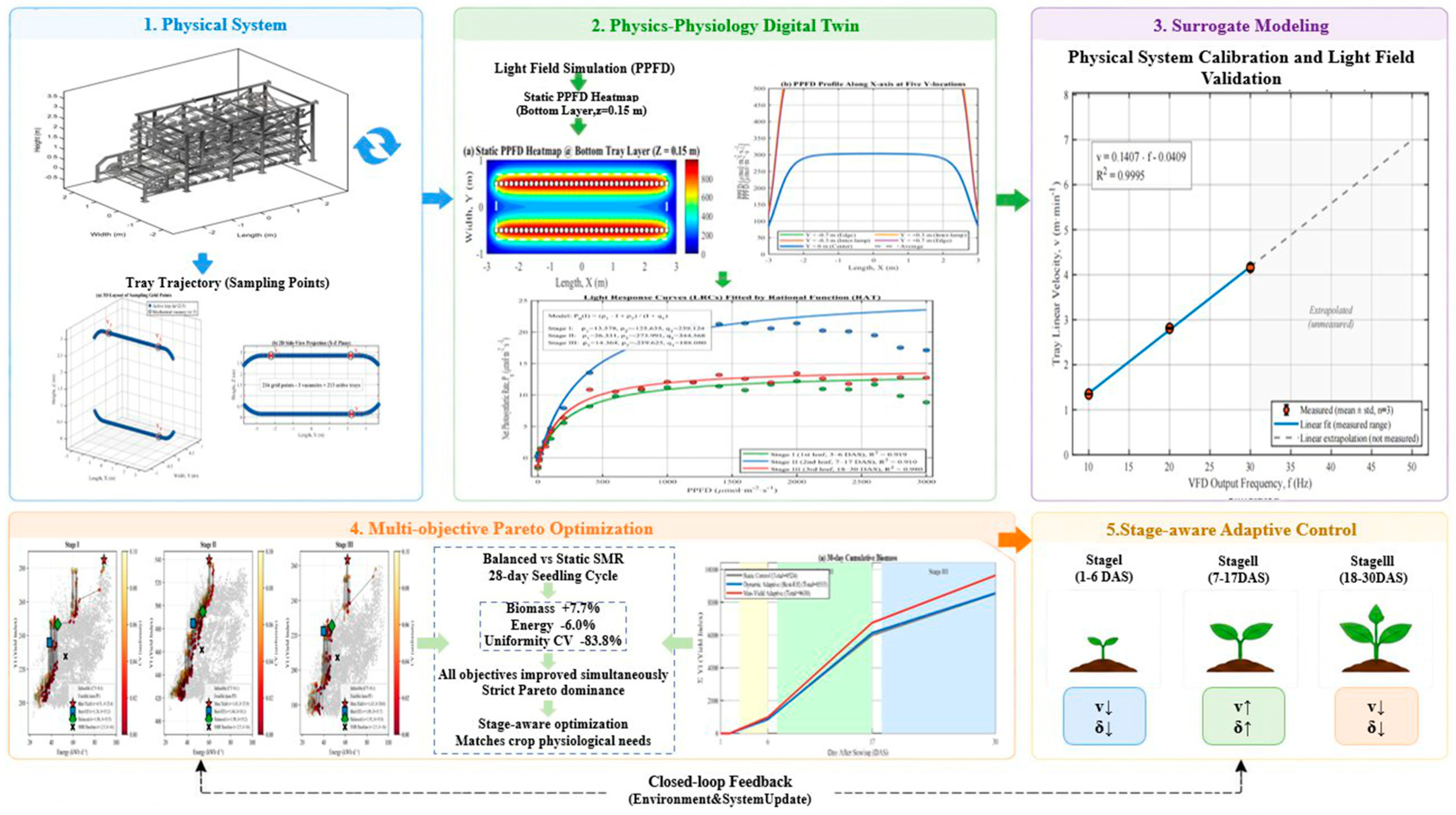
The overall research framework, which couples the physics–physiology digital twin, the XGBoost surrogate, and the stage-aware adaptive control strategy into a closed-loop pipeline, is illustrated in Figure 1.

2. Materials and Methods

2.1. Physical System Configuration and Kinematic Modeling

This study was conducted using an industrial-scale vertical circulating seedling factory and cultivation rack at the Key Laboratory of Northeast Smart Agricultural Technology, Ministry of Agriculture and Rural Affairs of Northeast Agricultural University. The seedling factory adopts a Venlo-type glass greenhouse structure, covering a total area of 768 square meters, with dimensions of 32 m * 24 m. The eaves of the greenhouse are 5.9 m high, the ridge height reaches 7.5 m, and the height of the sink is also 5.9 m. The greenhouse is covered with silicon glass and is equipped with an external sunshade system and an internal insulation system. The system employs a chain-driven vertical circulation mechanism to carry 213 standard seedling trays. The main structure is constructed from galvanized square steel, with overall dimensions of 6.0 m (L) * 2.0 m (W) * 3.0 m (H), and the long side is oriented north–south. The drive system integrates a Delta MS300 vector-controlled variable frequency drive (VFD), enabling modeled linear speeds from 0 to 5 m·min⁻¹. Detailed specifications are listed in

Table 1. Equipment parameter specifications.

Parameter Category	Parameter Name	Value/Specification	Unit	Parameter Category	Parameter Name	Value/Specification	Unit
Physical Structure	Overall Dimensions (L × W × H)	6.0 × 2.0 × 3.0	m	Motion Control	Drive Mechanism Type	Chain-driven vertical circulation	—
	Main Material	Galvanized square steel	—		VFD Model	Delta MS300	—
	Tray Capacity	213	sets		Linear Speed Range	0–5.0	m·min−1
Sensing and Monitoring	Number of Discrete Sampling Points	216	points	Environmental Control	Number of LED Lamps	70	units
	Sampling Interval	10	s		Power per Lamp	30	W
					Beam Angle	60	°

. A MATLAB 2024a-based simulation model was used to compute the temporal evolution of the light field for a representative day (April and May of 2026) in Harbin, China (45°45′ N, 126°38′ E).

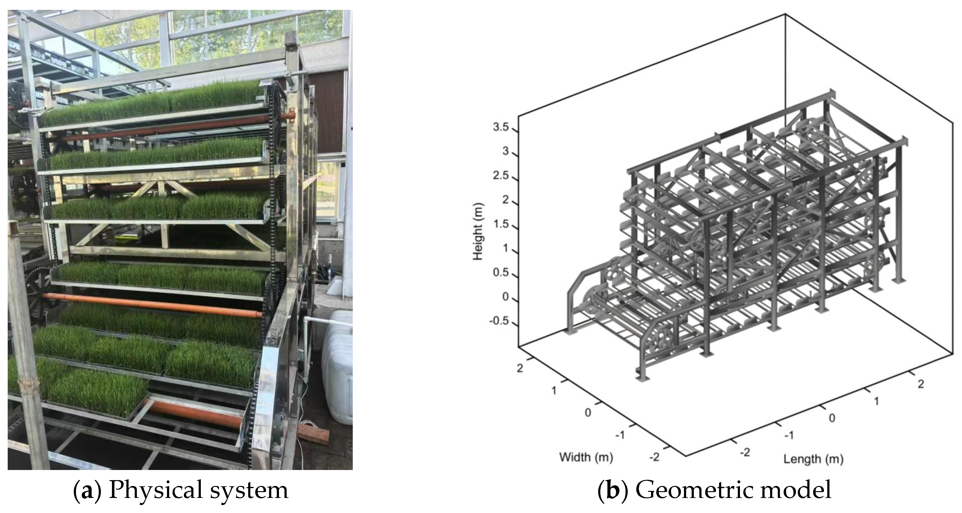
The physical system and its three-dimensional geometric abstraction are shown together in Figure 2. Figure 2 shows the physical rack and its three-dimensional geometric abstraction. Panel (a), shown on the left, presents the physical system, and panel (b), shown on the right, presents the geometric model. The rack is organized as six independently chain-driven cultivation layers that carry the 213 standard trays through a continuous closed-loop trajectory and periodically pass each tray through the bottom-mounted supplemental lighting zone.

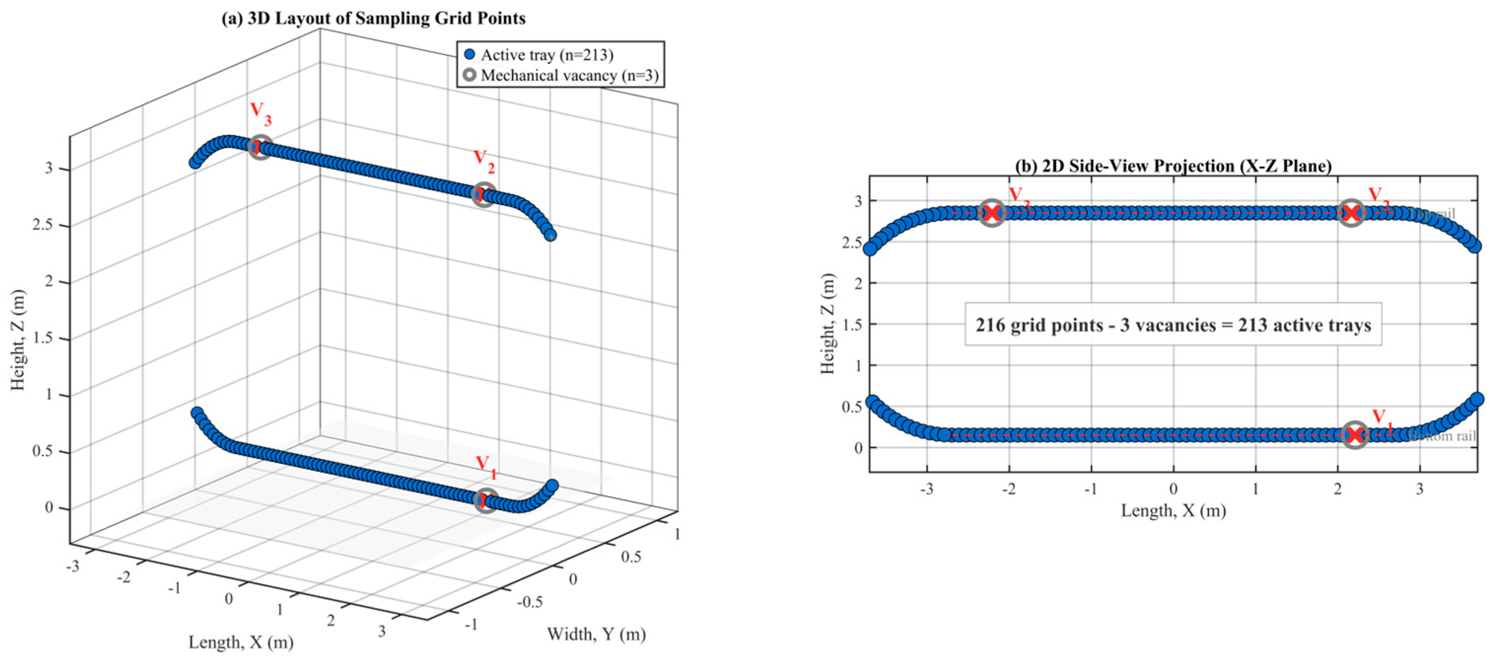
Due to geometric constraints imposed by the top and bottom rotating mechanisms, the spatial distribution of cultivation points is not strictly equidistant. To ensure high fidelity between the digital twin and the physical system, precise discrete coordinate mapping was performed for all 213 tray positions based on actual installation geometry, as shown in Figure 3.

A three-dimensional Cartesian coordinate system (XYZ), with the geometric center of the bottom drive shaft as the origin, was established to quantify dynamic light exposure during motion. Each tray is simplified as a centroid point, and its spatiotemporal trajectory along the chain is defined as Equation (1). The trajectory is parameterized by chain arclength s (m), with linear speed v (m·min⁻¹), angular speed $\mathit{\omega }\mathit{=}{\displaystyle \frac{\mathit{v}}{\mathit{R}}}$ (rad·min⁻¹) on curved sections, and tray spacing determined by the 216 modeled slots with 3 vacant positions, and cycle time $T_{cycle}={\displaystyle \frac{L_{total}}{v}}$.

$$\begin{array}{c}{x}_i\left(t\right)=X_{i,fixed}\\ y_i\left(t\right)=R·\sin \left(\omega t+{\phi }_{i,\theta }\right)\\ z_i\left(t\right)=Z_{offset}+R·\cos \left(\omega t+{\phi }_{i,\theta }\right)\end{array}$$

(1)

With ${\mathit{z}}_{\mathit{t}\mathit{o}\mathit{p}}=2.85\hspace{0.17em}\mathrm{m}$, ${\mathit{z}}_{\mathit{b}\mathit{o}\mathit{t}}=0.15\hspace{0.17em}\mathrm{m}$, ${\mathit{x}}_{\mathit{m}\mathit{i}\mathit{n}}=-2.70\hspace{0.17em}\mathrm{m}$, ${\mathit{x}}_{\mathit{m}\mathit{a}\mathit{x}}=2.70\hspace{0.17em}\mathrm{m}$, $R=1.35\hspace{0.17em}\mathrm{m}$, ${\mathit{L}}_{\mathit{h}\mathit{o}\mathit{r}\mathit{i}\mathit{z}\mathit{o}\mathit{n}\mathit{t}\mathit{a}\mathit{l}}=x_{\mathrm{m}\mathrm{a}\mathrm{x}}-x_{\mathrm{m}\mathrm{i}\mathrm{n}}$, and ${\mathit{L}}_{\mathit{t}\mathit{o}\mathit{t}\mathit{a}\mathit{l}}=2L_{\mathrm{h}\mathrm{o}\mathrm{r}\mathrm{i}\mathrm{z}\mathrm{o}\mathrm{n}\mathrm{t}\mathrm{a}\mathrm{l}}+2\pi R$, arclength_to_xyz maps $s$ to: (i) a lower straight segment $\mathit{x}\mathit{=}{\mathit{x}}_{\mathit{m}\mathit{i}\mathit{n}}\mathit{+}\mathit{s}$, $\mathit{z}\mathit{=}{\mathit{z}}_{\mathit{b}\mathit{o}\mathit{t}}$; (ii) a semicircular upper transition $\mathit{x}\mathit{=}{\mathit{x}}_{\mathit{m}\mathit{a}\mathit{x}}\mathit{+}\mathit{R}\mathit{s}\mathit{i}\mathit{n}\left(\mathit{\theta }\right)$, $\mathit{z}\mathit{=}{\mathit{z}}_{\mathit{c}\mathit{t}\mathit{r}}\mathit{-}\mathit{R}\mathit{c}\mathit{o}\mathit{s}\left(\mathit{\theta }\right)$; (iii) an upper straight segment $\mathit{x}\mathit{=}{\mathit{x}}_{\mathit{m}\mathit{a}\mathit{x}}\mathit{-}\left(\mathit{s}\mathit{-}{\mathit{L}}_{\mathit{h}\mathit{o}\mathit{r}\mathit{i}\mathit{z}\mathit{o}\mathit{n}\mathit{t}\mathit{a}\mathit{l}}\mathit{-}\mathit{\pi }\mathit{R}\right)$, $\mathit{z}\mathit{=}{\mathit{z}}_{\mathit{t}\mathit{o}\mathit{p}}$; and (iv) a semicircular lower transition $\mathit{x}\mathit{=}{\mathit{x}}_{\mathit{m}\mathit{i}\mathit{n}}\mathit{-}\mathit{R}\mathit{s}\mathit{i}\mathit{n}\left(\mathit{\theta }\right)$, $\mathit{z}\mathit{=}{\mathit{z}}_{\mathit{c}\mathit{t}\mathit{r}}\mathit{+}\mathit{R}\mathit{c}\mathit{o}\mathit{s}\left(\mathit{\theta }\right)$, where $\theta$ is $\mathrm{a}\mathrm{r}\mathrm{c}/R$ and ${\mathit{z}}_{\mathit{c}\mathit{t}\mathit{r}}\mathit{=}\left({\mathit{z}}_{\mathit{t}\mathit{o}\mathit{p}}\mathit{+}{\mathit{z}}_{\mathit{b}\mathit{o}\mathit{t}}\right)\mathit{/}\mathit{2}$. The numerical model uses $y=0$ for the chain centerline and advances $s$ modulo $L_{\mathrm{t}\mathrm{o}\mathrm{t}\mathrm{a}\mathrm{l}}$.

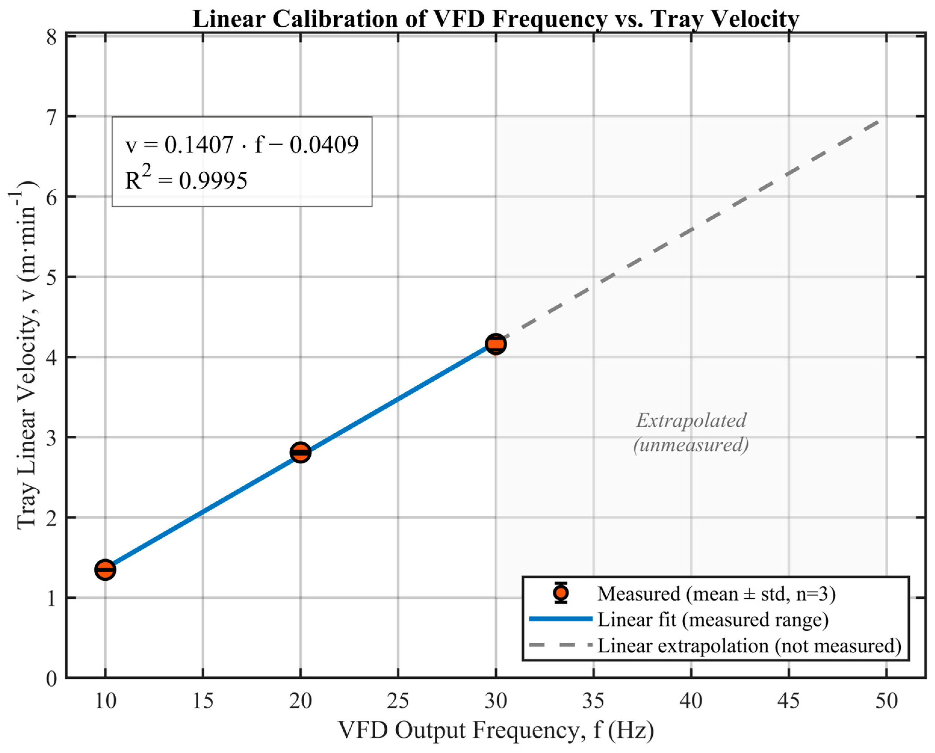
To eliminate nonlinear deviations in the mechanical transmission system, the mapping relationship between the driving motor frequency and the actual tray linear velocity $v$ was calibrated. High-precision displacement sensors were installed on both the drive shaft and the terminal chain to measure and record steady-state displacement data under different operating frequencies.

2.2. Dynamic Light Environment Simulation Engine

The natural light module uses a solar position calculation to obtain solar elevation over time. The model can be written as Equation (2), where ${\mathit{I}}_{\mathit{e}\mathit{x}\mathit{t}}\left(\mathit{t}\right)$ is outdoor PPFD (μmol·m⁻²·s⁻¹), $\tau$ is greenhouse transmittance (implemented as 0.64), f(${\mathit{\theta }}_{\mathit{z}}$) is a dimensionless structural shading correction, and ${\mathit{\theta }}_{\mathit{z}}$ is the solar zenith angle.

$$I_{sun}\left(t\right)=I_{ext}\left(t\right)·\tau ·f\left({\theta }_z\right)$$

(2)

In addition, Gaussian random perturbation ε ~ N (0, σ²) was introduced to simulate short-term irradiance fluctuations caused by cloud movement, thereby enhancing the robustness of the optimization framework under variable weather conditions. In the current implementation, ε(t) is simulated as a Gaussian perturbation with nominal standard deviation scale σ = 0.05 and a lower bound on the multiplicative factor.

For the implementation-consistent configuration of 70 bottom-mounted 30 W lamps, the supplemental PPFD is modeled as Equation (3), where I₀ = 350 μmol·m⁻²·s⁻¹ is the reference peak PPFD, z is the height, di = 0.30 m, di is the distance from lamp i to the receiving point, ${\mathit{\alpha }}_{\mathit{i}}$ is the incidence angle, and n = 2 is the beam exponent. Lamp positions use two rows with 35 positions per row and row offsets of −0.5 and +0.5 m.

$$I_{led}={\Sigma }_{i=1}^{70}{I}_0·{\left[z^2/\left(z^2+d_i^2\right)\right]}^{3/2}·co{s}^n\left({\alpha }_i\right)$$

(3)

The net carbon quantity over one day can be written as a light/dark carbon balance, shown in Equation (4), where P_n is the net photosynthetic rate (μmol CO₂·m⁻²·s⁻¹), R_d is the dark respiration rate in the same units, and the integration limits are the supplemental/natural light and dark intervals.

$$P_{net}={\int }_{t_{light}}{P}_n\left(I\left(t\right)\right)dt-{\int }_{t_{dark}}\left|R_d\right|dt$$

(4)

The Yield Index (YI) is model-predicted biomass accumulation potential index. ${\mathit{Y}\mathit{I}}_{\mathit{r}\mathit{a}\mathit{w}}\mathit{=}\mathit{\hspace{0.17em}}{\mathit{\sum }}_{\mathit{t}}\mathit{\hspace{0.17em}}\overline{\mathit{I}}\mathit{\hspace{0.17em}}{\mathit{P}}_{\mathit{n}}\mathit{(}\mathit{I}\mathit{(}\mathit{t}\mathit{)}\mathit{)}\mathit{\hspace{0.17em}}\mathit{\delta }\mathit{\hspace{0.17em}}{\mathit{t}}_{\mathit{h}}$ and $\mathit{Y}\mathit{I}\mathit{=}\mathit{\hspace{0.17em}}{\mathit{Y}\mathit{I}}_{\mathit{r}\mathit{a}\mathit{w}}\mathit{\hspace{0.17em}}{\mathit{K}}_{\mathit{s}\mathit{t}\mathit{a}\mathit{g}\mathit{e}}\mathit{\hspace{0.17em}}{\mathit{M}}_{\mathit{p}\mathit{o}\mathit{p}}$, where ${\mathit{K}}_{\mathit{s}\mathit{t}\mathit{a}\mathit{g}\mathit{e}}$ is the stage scaling value and ${\mathit{M}}_{\mathit{p}\mathit{o}\mathit{p}}$ is the population scaling value (implemented as 10). The implementation values are ${\mathit{K}}_{\mathit{s}\mathit{t}\mathit{a}\mathit{g}\mathit{e}}=\hspace{0.17em}0.18$, 0.22, and 0.15 for Stages I–III.

2.3. Biological Response Model Construction

To validate the fidelity of the physical model under occluded conditions, a dynamic trajectory validation experiment was conducted using a PLA-500 multifunctional spectroradiometer (Everfine, Hangzhou, China). The sensor was fixed at the center position of a tray on the second layer of the rotating system, with a sampling frequency of 1 s, continuously recording light intensity fluctuations over a 120 s period under a VFD operating frequency of 30 Hz (corresponding to a linear velocity of approximately 4.18 m/min).

“Long-jing 31”, a japonica rice variety, was selected for this study due to its dominant cultivation share in Heilongjiang Province and highly stable seed yield, which ensures consistent and reproducible experimental conditions. The seedlings were cultivated in nutrient-rich soil at a sowing density of 125 g of seeds per tray, with soil pH maintained within the range of 4.5–5.5. After sowing, seedling trays were placed in the vertical cultivation system to ensure the continuous absorption of water and nutrients. LI-COR 6800 (LI-COR Biosciences, Lincoln, NE, USA) light response curves were measured for Stage I (3–6 DAS), Stage II (7–17 DAS), and Stage III (18–30 DAS). During data acquisition, the light response curve was measured using the PPFD gradient from high to low, with settings of 3000, 2800, 2600, 2400, 2200, 2000, 1800, 1600, 1400, 1200, 1000, 800, 600, 400, 200, 100, 60, 20, 10, and 0 μmol·m⁻²·s⁻¹. The flow rate of the leaf chamber was set to 500 μmol s⁻¹, the CO₂ concentration of the air in the leaf chamber was set to 400 μmol·mol⁻¹, the relative humidity of the air in the leaf chamber was set to 50%, the leaf temperature was set to 25 °C, and the ratio of red light to blue light was set to 75%/25%. Each light intensity point was balanced for 60 s, and the relative change in the net photosynthetic rate within 30 s was less than 5% as the steady-state criterion.

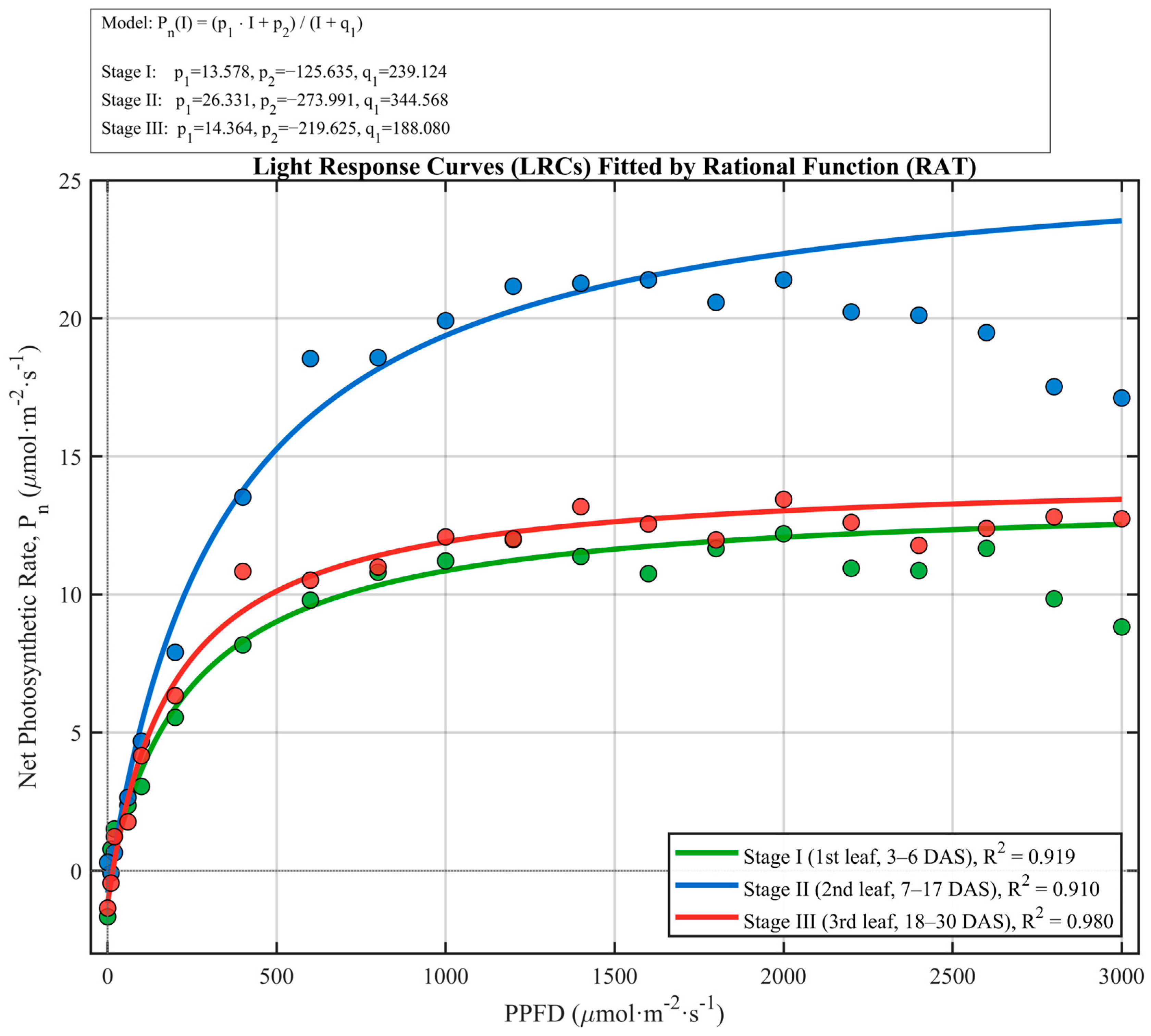
The stage-specific LRCs were fitted with a first-order rational (RAT) function and compared conceptually with RH and NRH alternatives. Figure 4 presents the photosynthetic light response curves fitted using a first-order rational function (RAT) model. In this study, three candidate models were compared: the rational function (RAT), the rectangular hyperbola (RH), and the non-rectangular hyperbola (NRH). The RH model exhibited substantial deviation in fitting nonlinear responses under high light intensity, while the NRH model frequently failed to converge when applied to datasets containing meteorological noise, limiting its suitability for automated optimization. In contrast, the RAT model demonstrated superior robustness and fitting accuracy, with Stage I $R^2=0.919$, Stage II $R^2=0.910$, and Stage III $R^2=0.980$, and is expressed as:

$$f\left(x\right)=\left(p_1·x+p_2\right)/\left(x+q_1\right)$$

(5)

where $p_1$ determines the asymptotic elevation of the curve, representing the potential to approach the maximum net photosynthetic rate ($P_n$), and $p_2/q_1$ corresponds to the dark respiration rate under zero irradiance. Based on this model, key physiological parameters such as dark respiration ($R_d=-p_2/q_1$) and the light compensation point (LCP) can be derived, providing a biological basis for evaluating the return on light energy input in subsequent control strategies. Since the $P_n$ values measured by the LI-COR 6800 are at the single-leaf scale, whereas the present study targets a population of 213 densely arranged trays, a stage-dependent population scaling factor $K_{\mathrm{stage}}$ was introduced in the biomass prediction framework. This factor was calibrated according to the dynamic expansion of the leaf area index (LAI) across the three developmental stages, enabling the model to capture scale effects in the transition from leaf-level photosynthesis to canopy-level biomass production. By incorporating $K_{\mathrm{stage}}$, the model effectively compensates for variations in canopy light interception due to plant development, allowing the Yield Index (YI) to reflect the cumulative dry matter production potential at the population level.

2.4. XGBoost Surrogate Model

The aforementioned physical–physiological coupled model involves high-fidelity dynamic trajectory integration, resulting in substantial computational cost for a single full-scenario simulation, which makes it impractical for the tens of thousands of iterations required in multi-objective optimization. To address the trade-off between search efficiency and computational accuracy, the Extreme Gradient Boosting (XGBoost) algorithm was introduced to construct a surrogate model [27].

The simulation dataset contained 1000 samples with 327, 307, and 366 samples in Stages I, II, and III, respectively. Inputs were speed, duration, and stage; targets were the YI (yield), energy, and CV. The surrogate model was trained using an 80/20 split, random_state = 2026, five-fold shuffled cross-validation with the same seed, and XGBoost settings of n_estimators = 300, max_depth = 6, learning_rate = 0.05, subsample = 0.85, and colsample_bytree = 0.85. Sampling bounds were defined as follows: rotational linear velocity $v\in \left[0.1, 5.0\right]$ m·min⁻¹ and daily supplemental lighting duration $\delta \in \left[10, 24\right]$ h/d, covering the full growth cycle of rice seedlings across three developmental stages. Corresponding response variables—including biomass accumulation potential (Yield Index, YI), energy consumption, and uniformity (CV)—were obtained using the MATLAB-based numerical simulation engine. The total system energy consumption $E_{\mathrm{total}}$ is defined as:

$$E_{total}=N·P_{led}·T_{light}/1000+{\int }_0^{24}{P}_{rated}·{\left(v/v_{max}\right)}^{k}dt$$

(6)

where $N=70$, $P_{\mathrm{led}}=30$ W, and $k=1.3$ is a proportional coefficient representing the combined effects of mechanical damping and transmission losses in the VFD-driven vertical circulating seedling cultivation rack. The energy model in the implementation is shown as Equation (6), where ${\mathrm{T}}_{\mathrm{l}\mathrm{i}\mathrm{g}\mathrm{h}\mathrm{t}}$ is the actual supplemental light operating duration (h/d), ${\mathrm{P}}_{\mathrm{l}\mathrm{e}\mathrm{d}}$ and ${\mathrm{P}}_{\mathrm{r}\mathrm{a}\mathrm{t}\mathrm{e}\mathrm{d}}$ are in W, ${\mathrm{v}}_{\mathrm{m}\mathrm{a}\mathrm{x}}$ = 5.0 m·min⁻¹, and k = 1.3.

During preprocessing, stage was treated as a categorical variable. The surrogate model workflow used the 80/20 split, random seed, five-fold procedure, and hyperparameters described above. XGBoost achieved scores of $R^2=0.9955$, RMSE = 8.12, and MAE = 5.40 on the test set, with a five-fold cross-validation $R^2=0.9933\pm 0.0024$, demonstrating excellent fitting accuracy and generalization stability. The final hyperparameters were determined as follows: maximum tree depth = 6, learning rate = 0.05, number of iterations = 300, subsample ratio = 0.85, and column sampling ratio = 0.85.

2.5. Multi-Objective Coordinated Control and Robust Optimization

To balance the trade-off between biomass accumulation potential and resource input costs in the vertical circulating seedling cultivation rack, a multi-objective optimization model was formulated as:

$$minF\left(v,\delta \right)=\left[f_1\left(v,\delta \right),f_2\left(v,\delta \right)\right]$$

(7)

subject to:

$$g\left(v,\delta \right)=CV\left(v,\delta \right)-0.10\le 0$$

(8)

where $f_1$ is defined as the negative value of net photosynthetic production (so that minimizing $f_1$ corresponds to maximizing biomass accumulation potential), and $f_2$ represents the total system energy consumption. The decision variables $v$ and $\delta$ denote the rotational linear velocity and daily supplemental lighting duration, respectively. The constraint function $g\left(v,\delta \right)$ ensures that the coefficient of variation (CV) of seedling uniformity remains below the threshold of 0.10, corresponding to the engineering upper limit for acceptable population non-uniformity in industrial seedling production. CV is defined in the simulator as the spatial coefficient of variation of each tray’s cumulative PPFD over non-overlapping 10 min windows during LED-on periods, averaged over selected windows: $\mathrm{C}\mathrm{V}=\hspace{0.17em}{\mathrm{m}\mathrm{e}\mathrm{a}\mathrm{n}}_w\left[{\displaystyle \frac{{\mathrm{s}\mathrm{t}\mathrm{d}}_i\left(C_{i,w}\right)}{{\mathrm{m}\mathrm{e}\mathrm{a}\mathrm{n}}_i\left(C_{i,w}\right)}}\right]$, where $C_{i,w}=\hspace{0.17em}{\sum }_t\hspace{0.17em}{I}_{i,t}\hspace{0.17em}\Delta \hspace{0.17em}t$. $\mathrm{C}\mathrm{V}\le 0.10$ is retained as an engineering screening threshold.

Leveraging the fast inference capability of the XGBoost surrogate model, a grid search strategy was adopted. The decision space was discretized into a 100 × 100 grid, generating 10,000 candidate control vectors for rapid evaluation, followed by identification of non-dominated solutions based on the Pareto dominance criterion. To account for operational uncertainties, Monte Carlo simulations were conducted to model potential ±5% fluctuations in motor speed during actual operation, and only solutions that maintained low output variability under such perturbations were retained. Based on the convergence characteristics of the Pareto front, two representative control strategies were extracted for the three developmental stages of rice seedlings: the “maximum biomass accumulation strategy” and the “optimal efficiency strategy”. A simulation-based stage-weighted comparison was used with Stage I = 3–6 DAS (4 days), Stage II = 7–17 DAS (11 days), and Stage III = 18–30 DAS (13 days): ${YI}_{28}=\hspace{0.17em}{\sum }_{\mathrm{s}}\hspace{0.17em}{d}_{\mathrm{s}}\hspace{0.17em}{YI}_{\mathrm{s}}$, $E_{28}=\hspace{0.17em}{\sum }_{\mathrm{s}}\hspace{0.17em}{d}_{\mathrm{s}}\hspace{0.17em}{E}_{\mathrm{s}}$, and ${CV}_{28}=\hspace{0.17em}{\displaystyle \frac{{\sum }_{\mathrm{s}}\hspace{0.17em}{d}_{\mathrm{s}}\hspace{0.17em}{CV}_{\mathrm{s}}}{28}}$.

To support cross-stage comparison of strategies, a consistent aggregation rule was defined. The total energy consumption $E_{\mathrm{total}}$, as defined in Equation (6), is obtained by integrating over a 0–24 h period, with units of kWh·d⁻¹ (daily energy consumption). Accordingly, the “three-stage total energy consumption” reported in subsequent sections refers to the arithmetic sum of the representative daily energy consumption across the three stages (kWh·d⁻¹), while the cross-stage aggregates of YI and CV are computed as simple arithmetic means. This choice of arithmetic aggregation, rather than weighting by stage duration, is justified for two reasons: first, all stage-specific LRC parameters ($p_1,p_2,q_1$) and the population scaling factor $K_{\mathrm{stage}}$ have already been fully encoded into the stage-wise YI responses during surrogate model training, meaning that each stage’s YI inherently captures its physiological contribution; applying additional duration-based weighting would therefore result in double counting. Second, the use of arithmetic aggregation ensures that energy-saving ratios and YI trade-offs remain independent of the specific length of the seedling cycle, allowing comparisons to be interpreted on a “per representative day” basis and facilitating transferability across different production scenarios. Under this unified aggregation framework, daily energy savings can be converted into total cycle savings by multiplying by the actual production duration without introducing inconsistency.

3. Results

3.1. Physical System Calibration and Light Field Validation

This subsection presents three categories of validation results that establish the credibility of the digital twin pipeline before any optimization is performed: (i) the variable frequency drive (VFD) frequency–velocity calibration that grounds the kinematic model in measured data; (ii) the simulated static PPFD distribution at the bottom cultivation layer that quantifies the spatial heterogeneity to be mitigated by rotation; and (iii) the dynamic trajectory comparison between the digital twin and PLA-500 in situ measurements that confirms the simulation engine reproduces the real light field statistics within 12% deviation.

Based on steady-state displacement measurements at three frequency setpoints (10, 20, and 30 Hz), linear regression yielded the relationship $v=0.1407f-0.0411(R^2=0.9995)$. As shown in Figure 5, the experimental results indicate a strong linear correlation between the VFD output frequency and the tray linear velocity. This calibrated relationship has been incorporated into the numerical model, ensuring that control commands generated by the optimization algorithm can be accurately implemented in practical operation.

It should be noted that the measured samples in Figure 5 cover a frequency range of $f\in \left[10, 30\right]$ Hz, corresponding to velocities of 1.35, 2.80, and 4.15 m·min⁻¹, within which the fitted relationship exhibits strong linearity. The maximum recommended velocity in subsequent optimization results (4.75 m·min⁻¹, corresponding to $f\approx 34$ Hz) slightly exceeds the measured range; this extrapolation is based on the commonly accepted engineering assumption of the near-linear torque–speed characteristic of VFD-driven motors within the nominal operating range (10–50 Hz), rather than direct experimental validation. In addition, the fitted intercept (−0.0411 m·min⁻¹, corresponding to $f^{*}\approx 0.29$ Hz at zero velocity) reflects the combined effects of startup inertia and transmission friction. This value is well below the typical minimum operating frequency of the VFD (≈1 Hz) and therefore does not affect the practical control range but should be interpreted as an engineering offset rather than a true physical zero point.

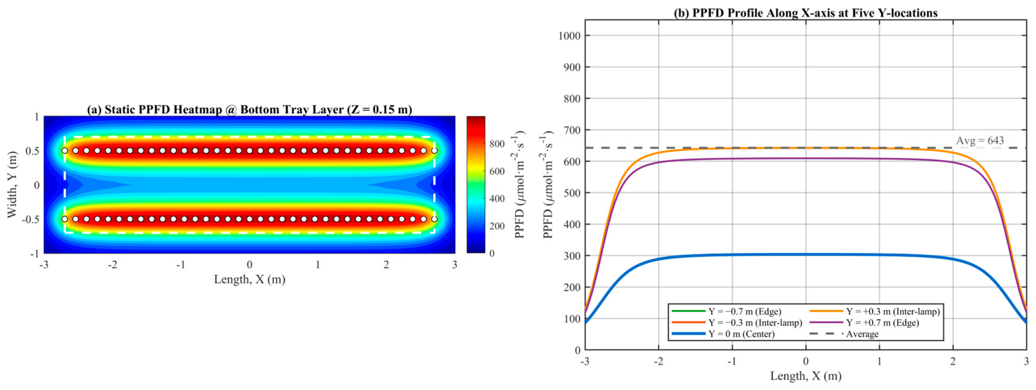
The average internal PPFD of the system was 643 μmol·m⁻²·s⁻¹, with a min/avg ratio of 0.278 (compared to 0.239 from DIALux industrial simulation) and a static coefficient of variation (CV) of 0.390, indicating strong consistency between the physical model and industrial-grade simulation in terms of spatial uniformity patterns. As illustrated in Figure 6, the static light field exhibits two key characteristics. First, along the width direction (y-axis), two parallel high-intensity bands are observed at $y\approx \pm 0.5$ m, with PPFD values of approximately 1250–1300 μmol·m⁻²·s⁻¹. A local minimum appears along the central corridor ($y=0$), with values around 950–1000 μmol·m⁻²·s⁻¹, while the outer edges ($\mid y\mid >0.9$ m) decline further to 450–600 μmol·m⁻²·s⁻¹. This spatial pattern directly reflects the geometric projection of the two rows of LED arrays: intensity peaks occur beneath the lamp axes, the central trough results from cosine attenuation between overlapping Lambertian distributions of adjacent fixtures, and the edge attenuation arises from unilateral light decay without compensatory overlap from the opposite side. Second, the peak-to-minimum difference reaches $\Delta \mathrm{PPFD}\approx 850$ μmol·m⁻²·s⁻¹, exceeding 65% of the peak value, corresponding to a static spatial CV of approximately 0.23–0.25 (computed along the width direction only, excluding the length-direction variance of 0.390 captured in the full-field CV reported above). This is substantially higher than the imposed engineering constraint of $CV\le 0.10$ in the optimization problem. This critical result indicates that, under a static cultivation configuration, there is virtually no engineering margin to achieve acceptable population uniformity without additional mechanical intervention. It therefore provides direct physical justification for introducing rotational motion as a temporal homogenization mechanism: by periodically redistributing trays across spatial gradients, rotation transforms spatial heterogeneity along the width direction into temporally averaged light exposure, thereby theoretically reducing the effective spatial CV.

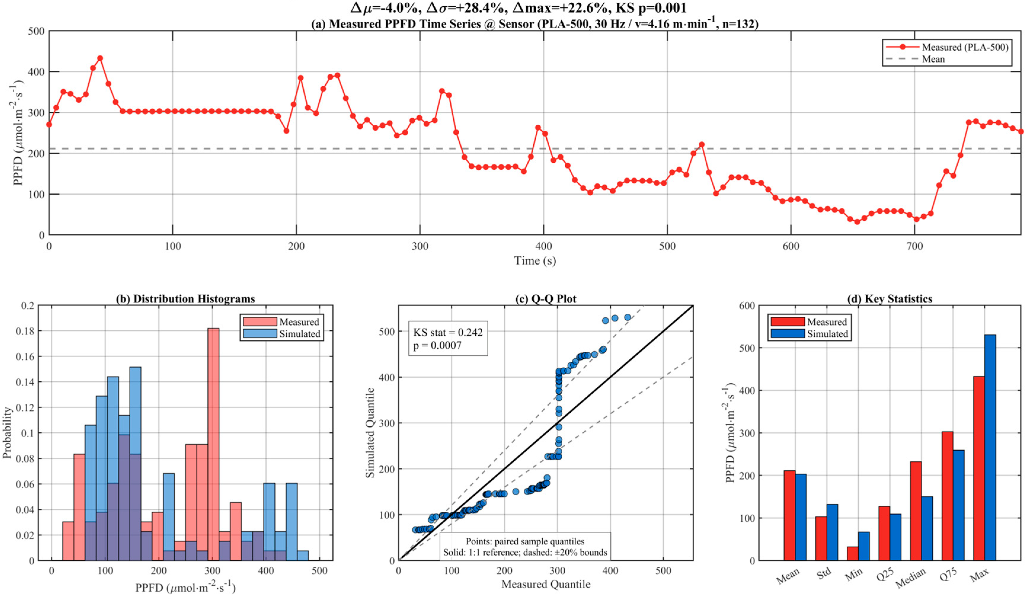
The statistical distributions of photosynthetic photon flux density (PPFD) obtained from the digital twin simulation and PLA-500 measurements are shown in Figure 7. Considering that the measured data contain non-stationary characteristics due to manual interruptions (e.g., the plateau observed between 60–180 s in Figure 7a), conventional pointwise R² evaluation is not applicable. Therefore, statistical distribution consistency was adopted for physical validation. The key statistical deviations are mean deviation Δμ = −3.4%, deviation in standard deviation Δσ = +20.8%, and maximum deviation Δmax = +11.4%. The Kolmogorov–Smirnov two-sample test yielded a KS statistic of 0.273 (p < 0.001). Although the null hypothesis of identical distributions is rejected at the α = 0.05 significance level, the magnitude of absolute deviations indicates that the simulation remains within 12% of the measurements in both mean and maximum values. The mean deviation between the two datasets is <6%, and the maximum deviation is <12%, confirming that the digital twin accurately reproduces the dynamic range of the light field under real operating conditions, thereby providing a reliable physical basis for subsequent optimization based on simulated data.

3.2. Dynamic Light–Photosynthesis Coupling and Cumulative Biomass

Building on the light field model and LRC measurements, this subsection examines simulation-derived quantities linking total PPFD to instantaneous Pn and compares model-predicted YI trajectories under static SMR, balanced adaptive, and max yield settings.

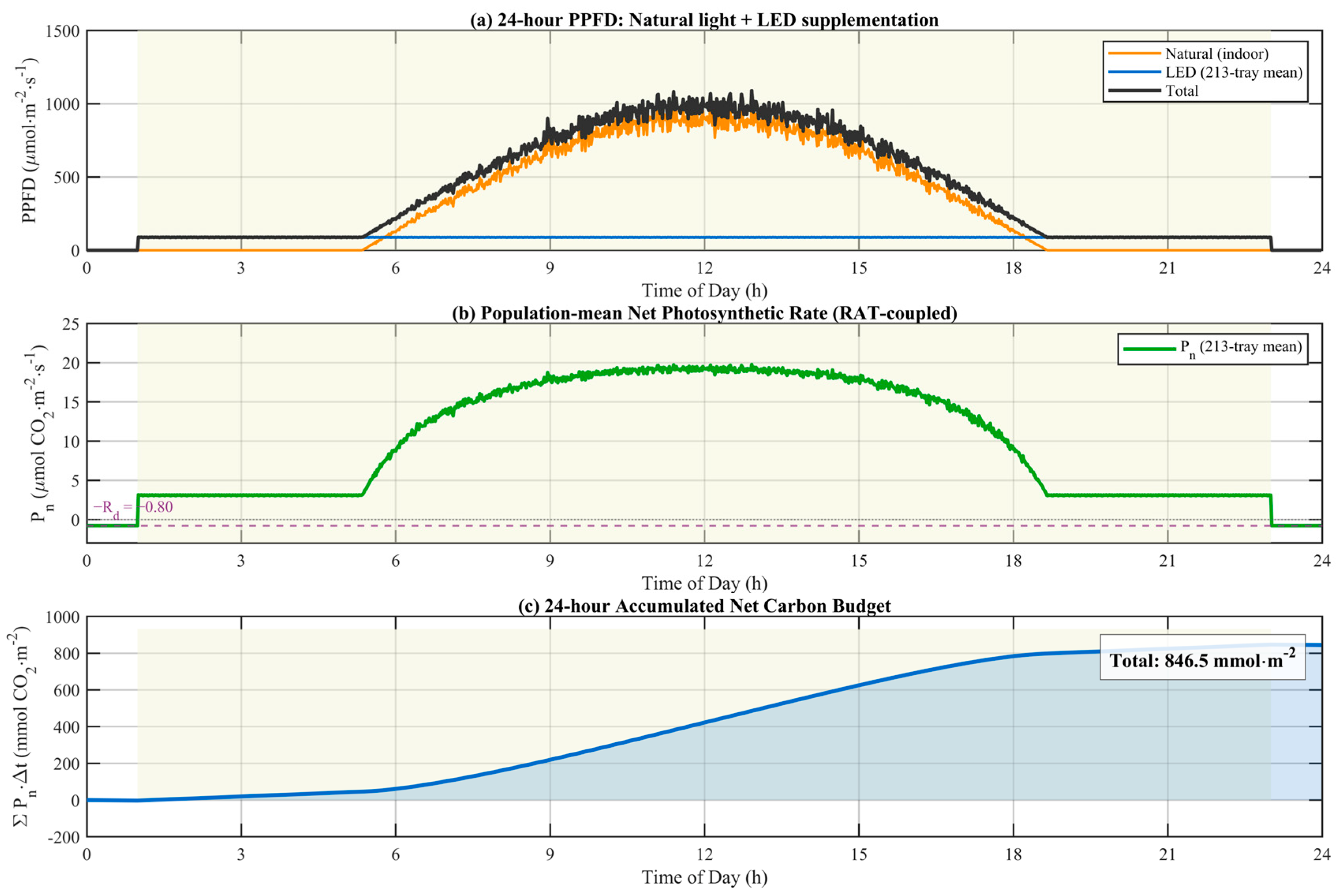
Figure 8 reveals the coupled dynamics of three signals over a 24 h period. The natural light component exhibits a typical bell-shaped profile, active from 05:00 to 19:00, with a peak of approximately 1200 μmol·m⁻²·s⁻¹. In contrast, LED supplemental lighting provides a constant baseline of about 200 μmol·m⁻²·s⁻¹ throughout the entire 0–24 h period. The superimposed total PPFD reaches a peak of nearly 1400 μmol·m⁻²·s⁻¹ around midday, significantly exceeding the light saturation point (LSP) indicated by the dashed line in the figure. The net photosynthetic rate $P_n$ (dense green band) exhibits high-frequency oscillations, with the oscillation frequency corresponding to the periodic rotation of the trays. The oscillation envelope shows strong nonlinear coupling with total PPFD: during nighttime periods (0–5 h and 19–24 h), when driven solely by LED lighting, $P_n$ remains at approximately 15 μmol CO₂·m⁻²·s⁻¹; during daytime, with the addition of natural light, it increases only slightly to about 18–19 μmol CO₂·m⁻²·s⁻¹, representing an increase of ~25%, whereas total PPFD simultaneously rises from ~200 to ~1400 μmol·m⁻²·s⁻¹ (a seven-fold increase). This pronounced nonlinear compression directly reflects the saturation characteristics of the light response curve (LRC) under dynamic conditions: even when total PPFD far exceeds the LSP, the marginal gain in $P_n$ remains minimal. From a physiological perspective independent of Pareto analysis, this phenomenon supports the rationale of the Stage III strategy described in Section 3.4, where reducing rotational speed achieves energy savings with a negligible loss in the YI. Furthermore, the maximum instantaneous amplitude of $P_n$ oscillations is approximately 5–6 μmol CO₂·m⁻²·s⁻¹ during daytime and increases to 8–10 μmol CO₂·m⁻²·s⁻¹ at night. The larger nighttime amplitude arises from the higher relative contrast between transient extrema under lower baseline conditions, whereas daytime oscillations are attenuated due to the saturation of the carbon assimilation capacity. This day–night asymmetry in oscillation amplitude may serve as a potential physiological indicator for the real-time detection of LRC saturation status in future closed-loop feedback control systems.

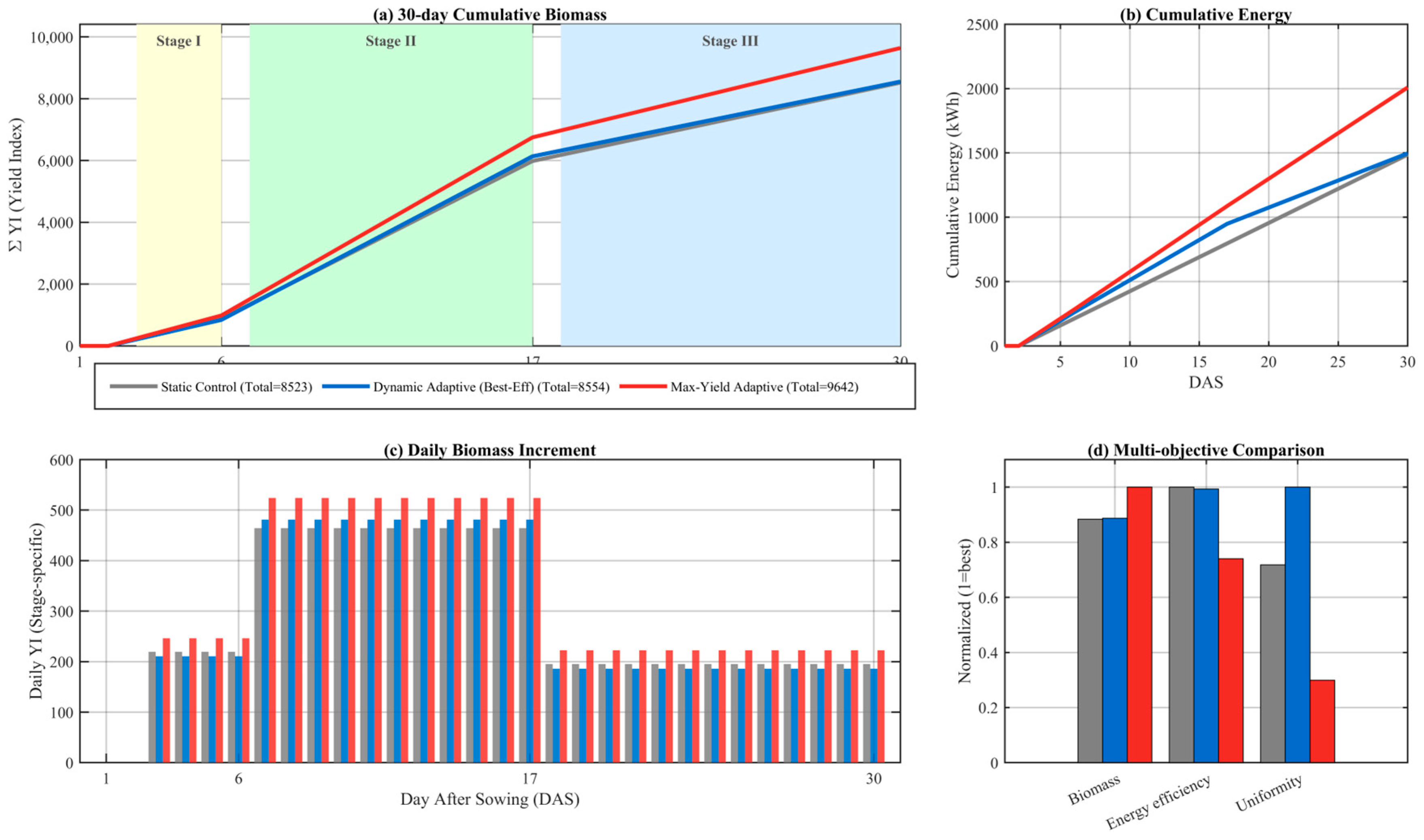
The simulated 28-day cumulative biomass curve (DAS 3–30) derived from time integration of the RAT light response model was presented in Figure 9, rather than from direct biological experiments. The computational workflow is as follows: the digital twin model provides total PPFD at each time step. The RAT light response model (Equation (5)) calculates the instantaneous net photosynthetic rate $P_n$ using stage-specific parameters ($p_1,p_2,q_1$); $P_n$ is integrated daily according to DAS. The result is scaled by the stage-dependent population factor $K_{\mathrm{stage}}$ to bridge from the single-leaf scale to the full population of 213 trays. Three strategies are compared: the static SMR baseline ($v=2.5$, $\delta =16$) yields a cumulative YI of 8682; the dynamic adaptive balanced strategy achieves a cumulative YI of 9353 (+7.7% relative to SMR); and the max yield strategy reaches 10,501 (+21.0% relative to SMR but with a +22.7% increase in energy consumption). Notably, the balanced strategy maintains a 6.0% reduction in cumulative energy consumption while achieving a higher daily YI across all three stages compared to the SMR baseline, thereby demonstrating strict Pareto dominance of stage-aware regulation over the static baseline.

3.3. Predictive Accuracy of the Surrogate Model

Table 2. Benchmark comparison of predictive performance across different algorithms.

Algorithm	Train R2	Test R2	Test RMSE	Test MAE	5-Fold CV R2
XGBoost (Proposed)	0.9998	0.9955	8.12	5.40	0.9933 ± 0.0024
Random Forest	1.0000	1.0000	0.29	0.21	1.0000 ± 0.0000
Gradient Boosting	1.0000	1.0000	0.30	0.20	1.0000 ± 0.0000
LightGBM	1.0000	1.0000	0.41	0.31	1.0000 ± 0.0000
Linear Regression	0.0460	0.0295	119.19	110.33	0.0369 ± 0.0158

Note: Random Forest, Gradient Boosting, and LightGBM show near-perfect values in the supplied table, which may reflect the discrete “stage” variable and the simulated data structure. XGBoost was retained with subsampling and column sampling, but this is not evidence of experimental generalization.

summarizes benchmarking on the unified simulated dataset. For the YI target, XGBoost has test R² = 0.9955, test RMSE = 8.12, test MAE = 5.40, and five-fold CV R² = 0.9933 ± 0.0024. These figures quantify surrogate prediction against simulation outputs; they do not validate measured yield or biomass.

Considering both predictive accuracy and generalization capability, XGBoost was selected as the surrogate model. By incorporating subsampling (subsample = 0.85) and column sampling (colsample_bytree = 0.85), the model maintains strong predictive performance while avoiding overfitting risks associated with tree-based ensembles under discrete-variable-dominated conditions. In addition, XGBoost achieves R² values exceeding 0.999 for both energy and CV prediction across the full dataset, satisfying the fidelity requirements for subsequent Pareto-based optimization.

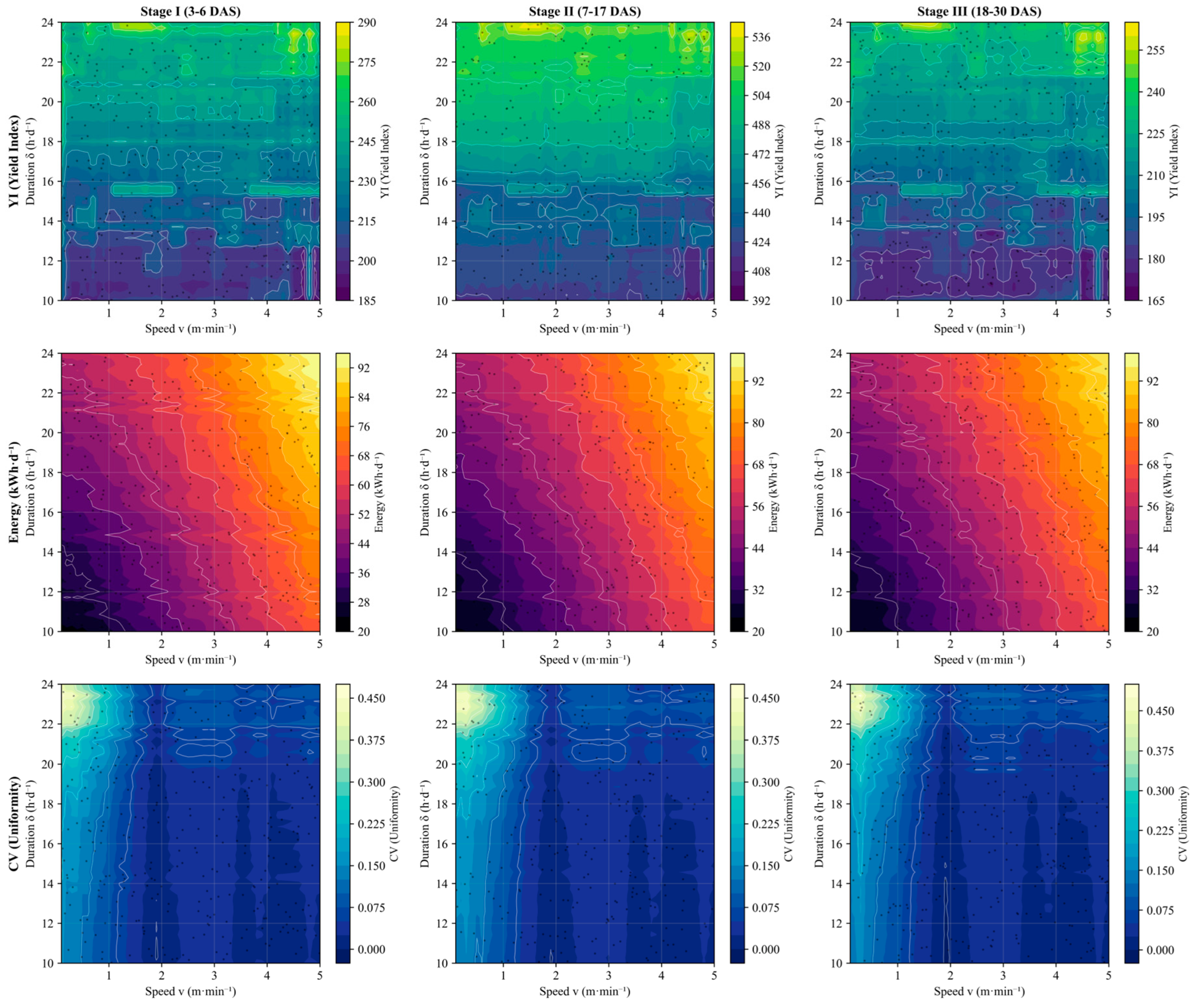
Figure 10 presents the complete dataset (1000 samples) generated by the digital twin simulations for training the machine learning surrogate model. The figure consists of two three-dimensional scatter plots, illustrating the global distributions of the YI and energy consumption within the parameter space spanned by rotational velocity $v$ and supplemental lighting duration $\delta$. Analysis of the YI response surface shows that high-yield regions do not occur at extreme values of maximum velocity or longest duration; instead, they are concentrated within a band characterized by moderate velocity and moderate duration, forming an approximate “ridge”-like optimal region. This non-uniform distribution is supported by two underlying physiological–physical mechanisms. First, when $\delta$ exceeds the equivalent integral corresponding to the light saturation point (LSP), additional light input enters the asymptotic region of the light response curve (LRC), where marginal gains in the YI approach zero. Second, excessively high $v$ reduces the residence time of seedlings within high-intensity LED zones to below the characteristic timescale of photosynthetic induction at the leaf level (2–5 min), leading to decoupling between light and dark reactions and consequently reducing carbon assimilation efficiency. These two mechanisms jointly shape the “ridge”-like optimal band in the parameter space. This geometric feature explains why linear regression and non-tuned SVR fail to capture the response surface, and also provides empirical justification for selecting XGBoost as the production surrogate model.

In contrast, the energy consumption response surface in Figure 10 exhibits a relatively monotonic pattern: energy consumption increases monotonically with $\delta$, while its dependence on $v$ is weaker but still positively correlated. This indicates that the supplemental lighting system, rather than the rotational drive, is the dominant contributor to energy consumption. The geometric discrepancy between the YI and energy response surfaces directly determines the non-trivial nature of the multi-objective optimization problem. If the two surfaces were geometrically similar, the Pareto front would degenerate into a near-linear relationship, allowing single-objective optimization to approximate the optimum. However, in this study, the misalignment between the YI ridge region and the monotonic energy gradient constitutes the geometric basis for uncovering non-intuitive strategies through stage-wise Pareto analysis (e.g., reducing rotational speed in Stage III to save energy with minimal loss in the YI). The nonlinear and multimodal characteristics of these response surfaces further justify the necessity of using tree-based ensemble learning methods such as XGBoost as surrogate models.

3.4. Stage-Wise Multi-Objective Pareto Optimization

Given the significant variation in resource requirements across different growth stages, constrained Pareto optimization was conducted separately for Stages I, II, and III. An engineering constraint of $CV\le 0.10$ was imposed to ensure population uniformity, representing the minimum acceptable standard for industrial seedling production; solutions exceeding this threshold were considered infeasible. The surrogate model generated 10,000 dense candidate points in the $\left(v\right|\delta )$ space ($v\in \left[0.1, 5.0\right]$ m·min⁻¹, $\delta \in \left[10, 24\right]$ h·d⁻¹), with feasible regions satisfying the CV constraint covering 78.4%, 79.2%, and 78.4% of the design space for Stages I, II, and III, respectively.

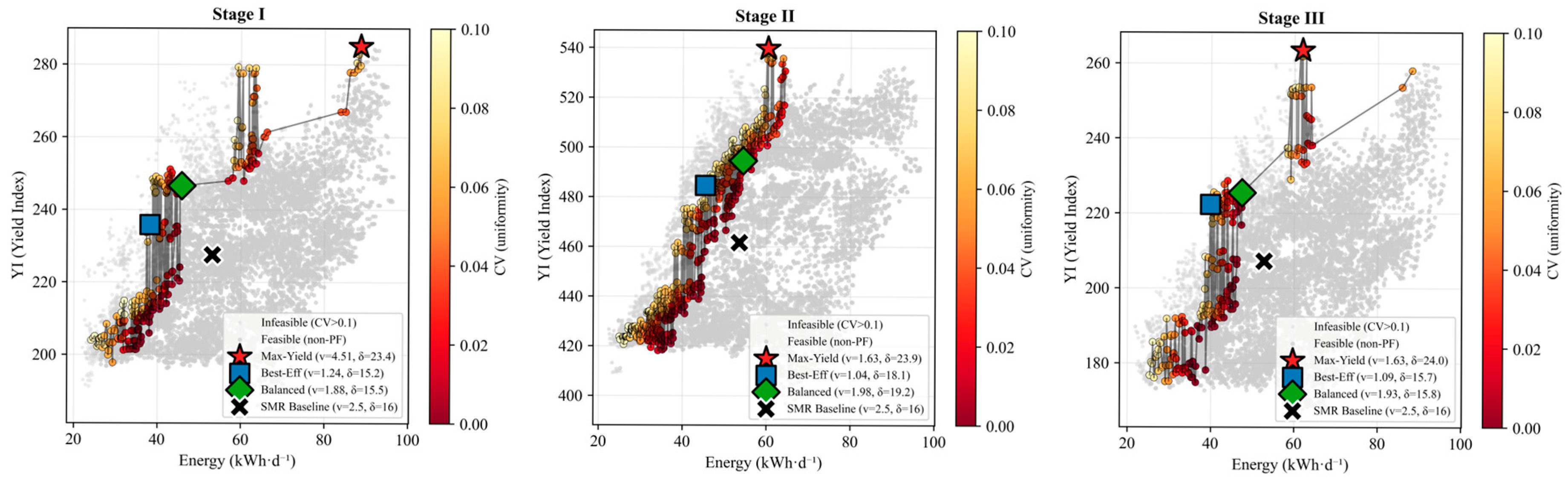
Figure 11 illustrates the geometric structure of the Pareto fronts for the three stages and their relative positions compared to the traditional SMR single-parameter baseline ($v=2.5$ m·min⁻¹, $\delta =16$ h·d⁻¹). Three representative strategies were extracted from the Pareto front: (1) max yield, which maximizes the YI within the CV-feasible region; (2) best efficiency, which minimizes energy consumption among solutions with a YI above the 60th percentile (Q60); and (3) balanced, which employs a normalized weighted utility function (weights: YI = 0.4, energy = 0.3, CV = 0.3). The specific parameters and performance metrics of these strategies are summarized in

Table 3. Derived management strategies.

Growth Stage	Strategy Type	Speed (m·min−1)	Lighting Duration (h)	Predicted Biomass Accumulation Potential (YI)	Energy Cost	Uniformity (CV)
Stage I	Max-Yield	4.51	23.43	285.0	88.67	0.0877
Stage I	Balanced	1.88	15.52	246.6	45.80	0.0045
Stage I	Best-Eff	1.24	15.23	235.8	38.17	0.0672
Stage II	Max-Yield	1.63	23.86	539.7	60.28	0.0890
Stage II	Balanced	1.98	19.19	494.6	54.39	0.0110
Stage II	Best-Eff	1.04	18.06	484.6	45.38	0.0949
Stage III	Max-Yield	1.63	24.00	263.4	61.95	0.0853
Stage III	Balanced	1.93	15.80	225.4	47.41	0.0019
Stage III	Best-Eff	1.09	15.66	222.3	39.86	0.0999

Note: the balanced, max yield, and best efficiency settings are candidate simulation strategies.

.

When aggregated over a 28-day seedling cycle (Stage I: 4 days; Stage II: 11 days; Stage III: 13 days), the balanced stage-adaptive strategy achieves simultaneous improvements across all three objectives relative to the SMR baseline: cumulative biomass increases by +7.7% (8682 to 9353 YI), daily energy consumption decreases by −6.0% (1486.4 to 1397.8 kWh), and the population-weighted average CV is reduced by −83.8% (0.0353 to 0.0058). All three objectives are improved concurrently, constituting strict Pareto dominance over the static baseline rather than a trade-off compromise. Detailed stage-wise comparisons are provided in

Table 4. Stage-wise comparison between the SMR baseline and the adaptive strategy.

Dimension	Stage/Aggregation	SMR Baseline	Adaptive Strategy	Relative Difference
Parameters (v, δ)	Stage I	(2.5, 16.0)	(1.88, 15.52)	—
	Stage II	(2.5, 16.0)	(1.98, 19.19)	—
	Stage III	(2.5, 16.0)	(1.93, 15.80)	—
Daily Energy Consumption (kWh·d−1)	Stage I	53.12	45.80	−13.8%
	Stage II	53.49	54.39	+1.7%
	Stage III	52.73	47.41	−10.1%
	28-day cumulative	1486.4	1397.8	−6.0%
YI	Stage I	227.6	246.6	+8.4%
	Stage II	461.6	494.6	+7.1%
	Stage III	207.2	225.4	+8.8%
	28-day cumulative	8681.9	9352.6	+7.7%
CV	Stage I	0.0360	0.0045	−87.5%
	Stage II	0.0342	0.0110	−67.8%
	Stage III	0.0357	0.0019	−94.7%
	28-day weighted average	0.0353	0.0058	−83.8%

Note: the supplied tables provide stage-wise model outputs.

.

Each subplot annotates the positions of the three strategies—max yield, best efficiency, and balanced—relative to the SMR baseline ($v=2.5$, $\delta =16$).

The three-stage Pareto fronts in Figure 11 exhibit systematic differences in geometric structure. In Stage I, the YI increases steeply within the low-energy region and then rapidly saturates, reflecting diminishing returns of additional light input for immature photosynthetic organs. In Stage II, the entire front shifts toward higher yield, with the highest YI gain per unit energy consumption among the three stages, corresponding to the optimal window of carbon assimilation efficiency. In Stage III, an “early turning point” emerges, where the YI approaches its upper limit at moderate energy levels, indicating the rapid decay of marginal returns following canopy closure. These stage-dependent geometric differences provide the most direct evidence for the effectiveness of stage-aware dynamic control and highlight the optimization space that fixed-parameter strategies inherently fail to capture.

The Pareto-dominant nature of the balanced strategy confers a structural rather than trade-off-based advantage over the SMR baseline: it significantly reduces population non-uniformity without increasing resource consumption, representing a key technical benchmark for transitioning industrial seedling production toward mechanized transplanting. The reduction of CV from 0.0353 to 0.0058 implies near-plant-level homogeneity within the population, an improvement that carries direct economic value for downstream mechanized operations such as automated seeding and batch transplanting. The max yield strategy (+21.0% biomass and +22.7% energy consumption) and the best efficiency strategy (−21.3% energy consumption and +5.6% biomass, with CV remaining within engineering constraints) provide alternative options under different cost structures: max yield for production scenarios prioritizing output, and best efficiency for energy-constrained conditions.

A side-by-side comparison of the SMR and balanced strategies across four dimensions—control parameters, daily energy consumption, YI, and CV—at each growth stage is presented in Table 4. In terms of parameters, the balanced strategy deviates from the fixed SMR setting (2.5, 16.0) in all three stages, with stage-specific adjustment patterns: supplemental lighting duration is reduced in Stage I and Stage III (δ ≈ 15.5–15.8 h), but is moderately extended in Stage II (δ = 19.19 h), reflecting differentiated lighting demands across developmental phases. From the perspective of daily energy consumption, Stage I and Stage III achieve energy savings of 13.8% and 10.1%, respectively, while Stage II shows a slight increase of 1.7%, resulting in a net cumulative energy saving of 6.0% over the 28-day cycle. In terms of the YI, all three stages exhibit consistent improvements ranging from 7.1% to 8.8%. The most pronounced effect is observed in CV, which shows dramatic reductions of 87.5%, 67.8%, and 94.7% across the three stages, respectively, with a weighted average decrease of 83.8%, from 0.0353 under SMR to 0.0058 under the balanced strategy, indicating near-plant-level homogeneity within the population. The simultaneous improvement across all three objectives demonstrates that the balanced strategy achieves strict Pareto dominance over the static SMR baseline, rather than a conventional trade-off. Based on the stage-specific mechanisms revealed in this comparison, the corresponding optimal operational settings for each stage can be further developed into operational recommendations for practical deployment.

3.5. Analysis of Factors Influencing Biomass Accumulation Potential Based on Shapley Values

To quantify the relative contributions of control variables to biomass accumulation potential (YI), this study employed the tree-based SHapley Additive exPlanations (TreeSHAP) method to evaluate feature importance in the XGBoost surrogate model (computed on the training dataset). Since the growth stage enters the YI calculation through two pathways, stage-specific LRC parameters ($p_1,p_2,q_1$) and the population scaling factor $K_{\mathrm{stage}}$, both of which act multiplicatively on the output, the stage variable is structurally assigned a higher sensitivity than other control variables. Therefore, the resulting SHAP ranking reflects not only the intrinsic contribution structure of the data but also the stage dependency embedded in the modeling pipeline, and these two aspects should be distinguished during interpretation.

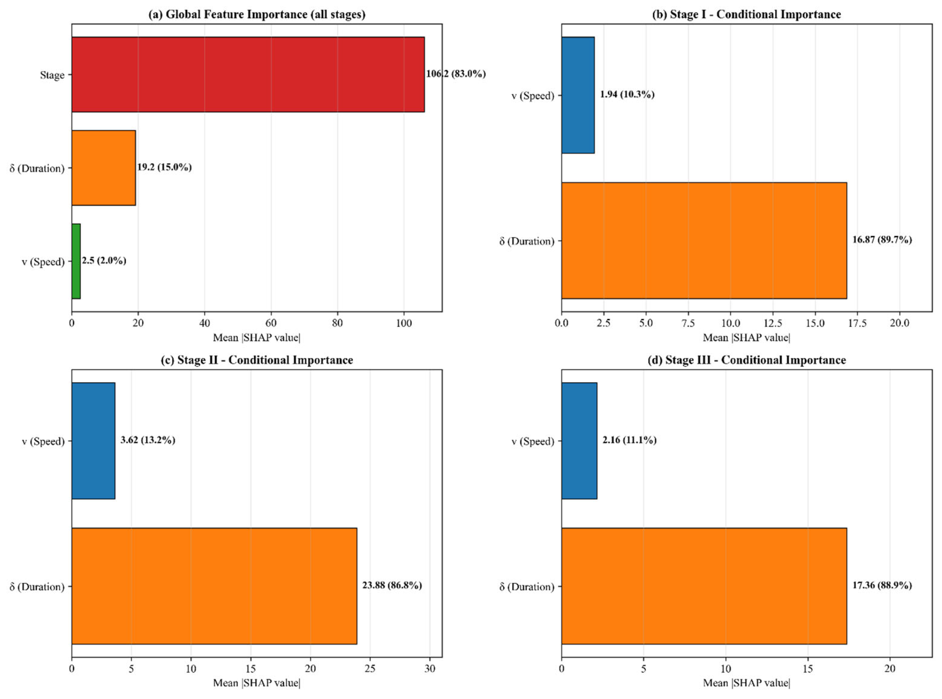
As shown in Figure 12, ((a) global scale (Stage 83.0%, $\delta$15.0%, $v$2.0%); (b)–(d) stage-conditioned results ($\delta$:$v$ ratios of 89.7:10.3, 86.8:13.2, and 88.9:11.1 for Stages I–III, respectively)), subfigure (a) presents global feature importance (mean |SHAP value|), ranking the average absolute contributions of growth stage (Stage), supplemental lighting duration (Duration), and rotational speed (Speed) across the full dataset. Subfigures (b)–(d) show stage-conditioned importance comparisons between $\delta$ and $v$: (b) Stage I (3–6 DAS), (c) Stage II (7–17 DAS), and (d) Stage III (18–30 DAS). While subfigure (a) highlights the dominant role of growth stage, subfigures (b)–(d) reveal how the relative importance of $\delta$ and $v$ evolves across developmental stages.

Global SHAP analysis indicates that growth stage contributes 83.0%, $\delta$ contributes 15.0%, and $v$ contributes 2.0%. This ranking reflects the structural property of the modeling pipeline, where the stage variable influences the YI through the multiplicative pathways of LRC parameters and $K_{\mathrm{stage}}$, demonstrating faithful capture of the predefined physical–physiological structure by the model. More decision-relevant insights arise from stage-conditioned SHAP analysis (Figure 12b–d): the contribution of $\delta$ is 89.7%, 86.8%, and 88.9% across Stages I–III, respectively, while the contribution of $v$ is 10.3%, 13.2%, and 11.1%. The relative contribution of $v$ peaks in Stage II (13.2%), indicating that this stage lies within the quasi-linear region of the light response curve (LRC), where variations in rotational speed most effectively modulate light fluctuation and photosynthetic response. In contrast, the influence of $v$ is constrained in Stages I and III due to boundary effects of the LRC (limited leaf area in Stage I and canopy closure in Stage III). This redistribution of variable importance within stages provides mechanistic evidence for stage-aware dynamic control strategies, independent of the Pareto front geometry.

4. Discussion

4.1. Coupling Mechanism Between the Light Environment and Net Photosynthetic Rate

The core concept of this study is to transform the spatial heterogeneity of light resources into temporal homogeneity through rotational motion. Simulation results indicate that, via the vertical circulation mechanism, seedlings periodically pass through artificial supplemental lighting zones and natural light zones. This spatiotemporal transformation can, to a certain extent, compensate for the uneven illumination caused by physical shading in traditional static cultivation systems. From a methodological perspective, digital twin technology provides a quantitative tool for this spatiotemporal coupling optimization by constructing a virtual replica of the physical system. This technology has been widely applied in crop monitoring, irrigation optimization, and greenhouse environment management [20,22], and this study further extends its application to the optimization of light environments in circulating seedling cultivation racks. It should be noted that a steady-state light response model is used for integration calculations. Since the system rotation cycle (in the order of minutes) is much longer than the induction time of photosynthetic electron transport (in the order of seconds), this quasi-steady-state approximation is considered reliable for macroscopic biomass estimation.

At the physiological level, dynamic light environments significantly influence the net photosynthetic rate of rice seedlings. Long et al. reported that the photosynthetic induction process under fluctuating light requires several minutes to reach steady-state efficiency, and carbon assimilation losses during light–dark transitions can reach 10–40% of the potential photosynthetic capacity [28]. Experimental data from this study similarly show that seedling responses to dynamic light pulses vary across growth stages. During Stage II (7–17 DAS), seedlings operate within the linear region of the light response curve (LRC), allowing efficient utilization of fluctuating light and resulting in rapid biomass accumulation. In contrast, during Stage III (18–30 DAS), canopy closure and self-shading effects reduce the marginal efficiency of light utilization. This observation is consistent with the findings of Slattery and Ort [29], who reported that light interception efficiency decreases with an increasing leaf area index (LAI) due to the exponential attenuation of light reaching lower canopy layers.

Although high-frequency light pulses can physically homogenize illumination, an excessive rotation speed may decouple light reactions from dark reactions at the physiological level [29]. It has been noted that carbon assimilation efficiency under fluctuating light is limited by the lag in photosynthetic induction; when light–dark switching occurs too rapidly, enzyme-driven dark reactions (e.g., RuBisCO activity) cannot respond in time. As a result, ATP and NADPH generated by light reactions are not fully utilized and may instead contribute to reactive oxygen species accumulation, potentially inducing photoinhibition [28]. Therefore, this study recommends reducing the rotation speed in later growth stages to extend the duration of individual light exposure events, allowing sufficient time for the Calvin cycle to utilize the generated chemical energy and achieve the stable accumulation of photosynthetic products. Due to the periodic stability of the mechanical structure and rotation trajectory, short-term light exposure validation can adequately characterize spatial shading patterns, while full-cycle physiological accumulation accuracy is ensured by the high-fidelity (R² = 0.98) light response model.

Future research will focus on experimentally validating the stage-aware parameter screening framework using sensor-based measurements and plant-based observations. Particular attention will be given to evaluating the transferability of the model across different cultivation conditions, its feasibility for computational deployment, and the biological stabilization of the controlled system. In addition, the effectiveness of physiological boundaries as screening constraints will be systematically investigated. Experimental studies will further assess whether these constraints can sufficiently prevent control saturation and abrupt actuator responses, or whether additional anti-windup and rate-limiting mechanisms are required for practical controller implementation.

4.2. Dynamic Control Paradigm Based on Physiological Feedback

The dynamic control framework proposed in this study shifts seedling environment management from experience-driven to physiology-driven decision-making. By integrating the stage-specific light response curves (LRCs) of rice seedlings (Stages I–III) with the physical motion parameters (v, δ) of the circulating seedling cultivation rack, this study establishes a quantifiable operational standard. The framework includes computational components with potential transferability, whereas the LRC parameters, LSP/LCP values, growth stage definitions, K_stage, and environmental calibration remain specific to the rice cultivar and cultivation site considered in this study. Future research will therefore focus on re-fitting these parameters and conducting systematic validation across different rice cultivars, crop species, and cultivation environments to assess the broader applicability and robustness of the framework.

From an engineering perspective, the key principle of this control framework is stage-wise adjustment of light input strategies. During Stage I, when photosynthetic organs are not fully developed and light utilization capacity is limited, an efficiency-oriented strategy is recommended, reducing rotation speed and supplemental lighting duration to control energy consumption. Stage II represents the period of highest carbon assimilation efficiency, where a high-yield strategy is appropriate to maximize light interception. In Stage III, canopy closure leads to increased self-shading and limited expansion of the effective photosynthetic area; thus, reducing linear speed and extending the duration of individual light exposure events can facilitate more effective utilization of photosynthetic products by the Calvin cycle, maintaining optimal seedling conditions prior to transplanting.

The nine strategies listed in Table 5 must be interpreted as triplets (YI, E, and CV); any comparison based on a single metric leads to systematic misjudgment. For example, in Stage II, the max yield strategy (YI = 539.7, E = 60.28 kWh·d⁻¹, CV = 0.0890) increases energy consumption by 10.8% compared to the balanced strategy (YI = 494.6, E = 54.39 kWh·d⁻¹, CV = 0.0110) while only achieving a 9.1% increase in the YI. However, CV decreases dramatically from 0.0890 to 0.0110 (a reduction of 87.6%), indicating that the balanced strategy achieves a fundamental improvement in population uniformity at the cost of a marginal yield reduction. This improvement has significantly higher downstream value for mechanized transplanting than marginal yield gains alone. Decision-making based solely on “energy cost per unit YI” would underestimate the production value of uniformity. A more rigorous framework should incorporate both “marginal energy cost per unit YI” (ΔE/ΔYI) and “energy cost per unit CV improvement” (ΔE/ΔCV), enabling producers to select strategies based on downstream willingness to pay for high-uniformity (low-CV) seedlings.

Table 5. Recommended management strategies by growth stage.

Growth Stage	Recommended Strategy	Recommended Speed V (m·min−1)	Recommended Duration δ (h)	Expected YI	Expected Energy (E)	Expected CV	Application Scenario
Stage I (3–6 DAS)	Balanced	1.88	15.52	246.6	45.80	0.0045	Uniformity prioritized in early seedling stage
Stage II (7–17 DAS)	Balanced	1.98	19.19	494.6	54.39	0.0110	Pareto-optimal during rapid growth stage
Stage III (18–30 DAS)	Balanced	1.93	15.80	225.4	47.41	0.0019	Low-energy, high-uniformity during robust seedling stage

Table 5. Recommended management strategies by growth stage.

Growth Stage	Recommended Strategy	Recommended Speed V (m·min−1)	Recommended Duration δ (h)	Expected YI	Expected Energy (E)	Expected CV	Application Scenario
Stage I (3–6 DAS)	Balanced	1.88	15.52	246.6	45.80	0.0045	Uniformity prioritized in early seedling stage
Stage II (7–17 DAS)	Balanced	1.98	19.19	494.6	54.39	0.0110	Pareto-optimal during rapid growth stage
Stage III (18–30 DAS)	Balanced	1.93	15.80	225.4	47.41	0.0019	Low-energy, high-uniformity during robust seedling stage

The proposed control scheme translates model assumptions into candidate motor speed and supplemental light duration settings. These settings are candidate simulation strategies and require experimental evaluation before operational deployment.

5. Conclusions

This study establishes a simulation-based framework integrating digital twin light field reconstruction, machine learning surrogate modeling, and multi-objective analysis for a vertical circulating rice seedling rack in cold regions in northeast China. The developed piecewise-trajectory digital twin quantitatively reconstructs the dynamic light environment along the circulating path, while the physics–physiology model links light exposure with stage-dependent photosynthetic responses. Based on the simulated dataset, the XGBoost surrogate model achieved high predictive performance for YI (test R² = 0.9955; five-fold CV R² = 0.9933 ± 0.0024), providing an efficient basis for parameter screening and multi-objective optimization.

Under the CV ≤ 0.10 engineering constraint, stage-wise optimization identified max yield, best efficiency, and balanced candidate operating settings, demonstrating that the preferred combinations of lighting duration and rack speed vary across growth stages rather than following a single fixed strategy. SHAP analysis further showed that stage was the dominant structural factor governing the simulated YI response, whereas duration and speed mainly contributed to within-stage variation. These findings indicate that stage-aware parameter adjustment is an important feature of the proposed optimization framework and provide quantitative guidance for balancing simulated yield potential, energy demand, and light distribution uniformity.

The present results are primarily simulation-based, and the available PLA-500 measurements provide only preliminary physical verification. Future research will therefore focus on broader PPFD validation, direct biomass and electrical energy measurements, LAI-based K_stage calibration, and closed-loop sensor feedback. The transferability of the framework to different rice cultivars and other crops will also be evaluated through parameter recalibration and experimental validation.

References

1. Despommier, D.D. The Vertical Farm: Feeding the World in the 21st Century; Macmillan: New York, NY, USA, 2010. [Google Scholar]
2. Graamans, L.; van den Dobbelsteen, A.; Meinen, E.; Stanghellini, C. Plant factories; crop transpiration and energy balance. Agric. Syst. 2017, 153, 138–147. [Google Scholar] [CrossRef] [Scilit]
3. Kozai, T.; Niu, G.; Takagaki, M. Plant Factory: An Indoor Vertical Farming System for Efficient Quality Food Production; Academic Press: London, UK, 2019. [Google Scholar]
4. Van Delden, S.H.; SharathKumar, M.; Butturini, M.; Graamans, L.J.A.; Heuvelink, E.; Kacira, M.; Kaiser, E.; Kromdijk, J.; Marcelis, L.F.M. Current status and future challenges in implementing and upscaling vertical farming systems. Nat. Food 2021, 2, 944–956. [Google Scholar] [CrossRef] [Scilit]
5. Asseng, S.; Guarin, J.R.; Raman, M.; Monje, O.; Kiss, G.; Despommier, D.D.; Meggers, F.M.; Gaber, P.P.G. Wheat yield potential in controlled-environment vertical farms. Proc. Natl. Acad. Sci. USA 2020, 117, 19131–19135. [Google Scholar] [CrossRef] [Scilit]
6. Kozai, T. Resource use efficiency of closed plant production system with artificial light: Concept, estimation and application to plant factory. Proc. Jpn. Acad. Ser. B 2013, 89, 447–461. [Google Scholar] [CrossRef] [Scilit]
7. Faust, J.E.; Logan, J. Daily light integral: A research review and high-resolution maps of the United States. HortScience 2018, 53, 1250–1257. [Google Scholar] [CrossRef] [Scilit]
8. Hemming, S.; de Zwart, F.; Elings, A.; Righini, I.; Petropoulou, A. Remote control of greenhouse vegetable production with artificial intelligence—Greenhouse climate, irrigation, and crop production. Sensors 2019, 19, 1807. [Google Scholar] [CrossRef] [Scilit]
9. Sarlikioti, V.; de Visser, P.H.B.; Buck-Sorlin, G.H.; Marcelis, L.F.M. How plant architecture affects light absorption and photosynthesis in tomato: Towards an ideotype for plant architecture using a functional-structural plant model. Ann. Bot. 2011, 108, 1065–1073. [Google Scholar] [CrossRef] [Scilit]
10. Li, Q.; Kubota, C. Effects of supplemental light quality on growth and phytochemicals of baby leaf lettuce. Environ. Exp. Bot. 2009, 67, 59–64. [Google Scholar] [CrossRef] [Scilit]
11. Guo, Y.; Zhao, H.; Zhang, S.; Wang, Y.; Chow, D. Modeling and optimization of environment in agricultural greenhouses for improving cleaner and sustainable crop production. J. Clean. Prod. 2022, 285, 124843. [Google Scholar] [CrossRef] [Scilit]
12. Bugbee, B. Toward an optimal spectral quality for plant growth and development: The importance of radiation capture. Acta Hortic. 2016, 1134, 1–12. [Google Scholar] [CrossRef] [Scilit]
13. Dresch, C.; Vidal, V.; Suchail, S.; Chevallier, O.; Sallanon, H.; Truffault, V.; Charles, F. A rotational cultivation system for indoor-grown lettuce: Feasibility in terms of yields, resource efficiency, quality, and postharvest storage capacity. Agronomy 2025, 15, 744. [Google Scholar] [CrossRef] [Scilit]
14. Yu, C.; Shang, M.; Cui, R.; Chen, J.; Zhou, S.; Du, X. Design and experiment of a rotating strawberry planting device with self-supplementary lighting. Trans. Chin. Soc. Agric. Eng. 2025, 41, 43–52. [Google Scholar] [CrossRef]
15. Paucek, I.; Pennisi, G.; Pistillo, A.; Appolloni, E.; Crepaldi, A.; Caber, S.; Magrefi, F.; Gianquinto, G.; Orsini, F. Supplementary LED interlighting improves yield and precocity of greenhouse tomatoes in the Mediterranean. Agronomy 2020, 10, 1002. [Google Scholar] [CrossRef] [Scilit]
16. Poorter, H.; Fiorani, F.; Pieruschka, R.; Wojciechowski, T.; van der Putten, W.H.; Kleyer, M.; Fischer, U.; Schurr, U. Pampered inside, pestered outside? Differences and similarities between plants growing in controlled conditions and in the field. New Phytol. 2016, 212, 838–855. [Google Scholar] [CrossRef] [Scilit]
17. Monostori, I.; Heilmann, M.; Kocsy, G.; Rakszegi, M.; Ahres, M.; Altenbach, S.B.; Szalai, G.; Pal, M.; Toldi, D.; Simon-Sarkadi, L.; et al. LED lighting—modification of growth, metabolism, yield and flour composition in wheat by spectral quality and intensity. Front. Plant Sci. 2018, 9, 605. [Google Scholar] [CrossRef] [Scilit]
18. Kaiser, E.; Kusuma, P.; Vialet-Chabrand, S.; Harbinson, J.; Heuvelink, E.; Marcelis, L.F.M. Vertical farming goes dynamic: Optimizing resource use efficiency, product quality, and energy costs. Front. Sci. 2024, 2, 1411259. [Google Scholar] [CrossRef] [Scilit]
19. Tao, F.; Zhang, H.; Liu, A.; Nee, A.Y.C. Digital twin in industry: State-of-the-art. IEEE Trans. Ind. Inform. 2019, 15, 2405–2415. [Google Scholar] [CrossRef] [Scilit]
20. Pylianidis, C.; Osinga, S.; Athanasiadis, I.N. Introducing digital twins to agriculture. Comput. Electron. Agric. 2021, 184, 105942. [Google Scholar] [CrossRef] [Scilit]
21. Alves, R.G.; Lima, F.; Guedes, I.M.R.; Gimenez, S.P. Dynamic light optimization in vertical farming using an IoT-driven digital twin framework and artificial intelligence. Appl. Soft Comput. 2025, 174, 112985. [Google Scholar] [CrossRef] [Scilit]
22. Pergner, I.; Lippert, C.; Piepho, H.-P.; Schwarz, J.; Kehlenbeck, H. How to determine temporal yield variances of various cropping systems for modelling farmers’ production risk–Illustrated by results from a long-term field trial. Eur. J. Agron. 2023, 152, 127005. [Google Scholar] [CrossRef] [Scilit]
23. Wang, L.; Li, Y.; Lin, H.; Zheng, L.; Wang, S.; Wu, J.; Li, T. RTR-CNN: Rotating tray region selection and seedling health status detection via CNN in greenhouse seedling beds. Comput. Electron. Agric. 2025, 229, 109723. [Google Scholar] [CrossRef] [Scilit]
24. Hildebrandt, G.; Dittler, D.; Habiger, P.; Drath, R.; Weyrich, M. Data integration of digital twins in industrial automation: A systematic literature review. IEEE Access 2024, 12, 139129–139153. [Google Scholar] [CrossRef] [Scilit]
25. Stevanović, S.; Dashti, H.; Milošević, M.; Al-Yakoob, S.; Stevanović, D. Comparison of ANN and XGBoost surrogate models trained on small numbers of building energy simulations. PLoS ONE 2024, 19, e0312573. [Google Scholar] [CrossRef] [Scilit]
26. Cheng, D.; Yao, Y.; Liu, R.; Li, T.; Li, D.; Chen, J. Precision agriculture management based on a surrogate model assisted multiobjective algorithmic framework. Sci. Rep. 2023, 13, 1142. [Google Scholar] [CrossRef] [Scilit]
27. Chen, T.; Guestrin, C. XGBoost: A scalable tree boosting system. In KDD ’16: The 22nd ACM SIGKDD International Conference on Knowledge Discovery and Data Mining; Association for Computing Machinery: New York, NY, USA, 2016; pp. 785–794. [Google Scholar]
28. Long, S.P.; Taylor, S.H.; Burgess, S.J.; Carmo-Silva, E.; Lawson, T.; De Souza, A.P.; Leonelli, L.; Wang, Y. Into the Shadows and Back into Sunlight: Photosynthesis in Fluctuating Light. Annu. Rev. Plant Biol. 2022, 73, 617–648. [Google Scholar] [CrossRef] [Scilit]
29. Slattery, R.A.; Walker, B.J.; Weber, A.P.M.; Ort, D.R. The impacts of fluctuating light on crop performance. Plant Physiol. 2018, 176, 990–1003. [Google Scholar] [CrossRef] [Scilit]
Figure 1. Overall research framework, comprising five integrated modules.
Agriculture 16 01930 g001
Figure 2. Vertical circulating seedling cultivation rack: (a) photograph; (b) 3D geometric model.
Agriculture 16 01930 g002
Figure 3. Spatial distribution of discrete PPFD sampling points across six cultivation layers.
Agriculture 16 01930 g003
Figure 4. Three-stage light response curves (LRCs) based on LI-COR 6800 measurements.
Agriculture 16 01930 g004
Figure 5. Linear calibration curve between VFD output frequency and tray linear speed.
Agriculture 16 01930 g005
Figure 6. Spatial distribution of static PPFD at the bottom layer (Z = 0.15 m) under 70 LED lamps.
Agriculture 16 01930 g006
Figure 7. Statistical distribution validation of photosynthetic photon flux density (PPFD) between digital twin simulation and PLA-500 measurements. Δμ = −3.4%, Δσ = +20.8%, Δmax = +11.4%, and KS p < 0.001 while absolute deviations remain below 12%. (a) Time series of 132 measured sampling points; (b) comparison of PPFD distribution histograms between measurements and simulations; (c) Q–Q plot showing quantile correspondence; and (d) key statistics comparison.
Agriculture 16 01930 g007
Figure 8. Graph showing the 24 h coupled time series of PPFD, Pn, and cumulative carbon balance under a representative condition (Stage II, v = 3.0 m·min−1, δ = 22 h·d−1, YI = 515.6).
Agriculture 16 01930 g008
Figure 9. Simulation-based comparison of the 28-day cumulative Yield Index (YI) under static SMR, dynamic adaptive balanced, and max yield settings.
Agriculture 16 01930 g009
Figure 10. Response surfaces of the XGBoost surrogate model in the (v, δ) decision space (3 stages * 3 objectives = 9 subplots for YI, energy, and CV).
Agriculture 16 01930 g010
Figure 11. Three-stage Pareto fronts and derived strategies under the engineering constraint of CV ≤ 0.10.
Agriculture 16 01930 g011
Figure 12. TreeSHAP feature importance. Note: The SHAP ranking is computed from the surrogate model and reflects the structure of the simulated training dataset. The global contribution of Stage is partly structural because Stage enters through stage-specific LRC parameters and K_stage.
Agriculture 16 01930 g012