Expert-Driven Spraying Phases and Deep Learning-Assisted Decision Support for Karshi/Qashqadaryo Irrigated Cotton Cultivation

Abstract

Accurate spray timing is essential for reducing unnecessary pesticide use in irrigated cotton production. This study developed and evaluated a locally calibrated six-stage Spraying Phase (SP) scale for the Karshi/Qashqadaryo production context. The scale was established through a two-round moderated consensus process involving 16 expert panelists representing this production context. A screened dataset of 14,400 non-standardized smartphone images was used to train and evaluate a ResNet-50 convolutional neural network (CNN) for SP-stage classification. Field validation was conducted at the Karshi Engineering and Economics Institute during the 2023 and 2024 seasons using an internally controlled randomized complete block design (RCBD)-style paired comparison of SP-based and BBCH-based spray timing. The CNN achieved 93.0% test accuracy. The mean number of pesticide applications was descriptively lower under SP-guided scheduling than under BBCH-based scheduling (3.75 versus 4.88 applications per season; −23.1%). For the inferentially evaluated outcomes, crop-protection cost decreased by 21.2%, the Environmental Risk Index decreased by 21.6%, and plot-level lint-equivalent yield increased by 4.5%. These findings support SP-guided timing as a promising locally calibrated decision-support approach under the tested Karshi/Qashqadaryo conditions; broader use requires multi-site, multi-cultivar, multi-season, device-stratified, and BBCH-level validation, together with technical deployment testing and implementation-cost assessment.

1. Introduction

Cotton remains an economically important crop in Central Asia and is a central component of irrigated agricultural systems in Uzbekistan [1,2]. At the same time, cotton is a high-input crop, and plant-protection decisions can strongly influence production cost, environmental risk, and farm-worker exposure [3,4]. Insect pests such as cotton bollworm (Helicoverpa armigera) and sap-sucking pests are particularly important in regional cotton systems, especially when warm summer conditions favor rapid pest development [5]. Integrated pest management (IPM), therefore, emphasizes timely, need-based interventions rather than routine prophylactic spraying [6].

Phenological timing is a practical constraint in cotton crop protection. The BBCH scale provides an internationally recognized system for describing cotton development [7] within the broader BBCH framework for mono- and dicotyledonous plants [8], but it is not designed as a local spray-decision scale. Broad BBCH stages may be sufficient for general communication, yet they do not always identify the field-visible intervention windows that advisers and growers use during pest-management decisions. This limitation is relevant in the Karshi/Qashqadaryo irrigated cotton context, where short growing seasons, furrow irrigation, local cultivar development, and seasonal pest pressure can narrow the useful spray window.

Computer vision offers a complementary way to operationalize phenological observation. Convolutional neural networks (CNNs) have been used to classify crop growth stages and extract phenological information from field imagery [9,10,11,12,13,14]. However, image-based tools require target classes that are agronomically meaningful, observable under routine field conditions, and sufficiently distinct for consistent labeling. A locally calibrated Spraying Phase scale can therefore connect expert agronomic knowledge with automated image classification. Decision-support models in crop protection provide a related example of linking biological risk or stage prediction with treatment timing [15].

A methodological challenge in image-based crop-stage recognition is that high test accuracy may partly reflect dataset-specific cues rather than transferable phenological recognition. Potential sources include farm or contributor background, soil and canopy context, device-specific color rendering, illumination, viewpoint, and uncertainty in expert labels. The present study, therefore, treated internal validity and transferability as separate issues: contributor-wise data partitioning, duplicate screening, independent SP-label validation, and cautious scope language were used to reduce overinterpretation of model performance.

The objective of this study was to develop and evaluate an expert-defined Spraying Phase (SP) scale for cotton spray-timing support under Karshi/Qashqadaryo irrigated production conditions. The study had three linked aims: (i) we define an operational SP scale through structured expert consensus; (ii) we train and validate a CNN model for SP-stage recognition from screened smartphone images; and (iii) we compare SP-guided timing with BBCH-based timing in a two-season field validation. The study was not designed to establish national representativeness; transferability beyond the tested context requires additional regional validation.

2. Materials and Methods

The study site and agronomic context are described first. The subsequent workflow consisted of four sequential components: expert consensus, smartphone image screening and labeling, CNN training and evaluation, and two-season field validation. These components linked the locally defined SP scale with image-based stage recognition and a controlled comparison of SP-based and BBCH-based spray timing.

2.1. Experimental Field and Agronomic Context

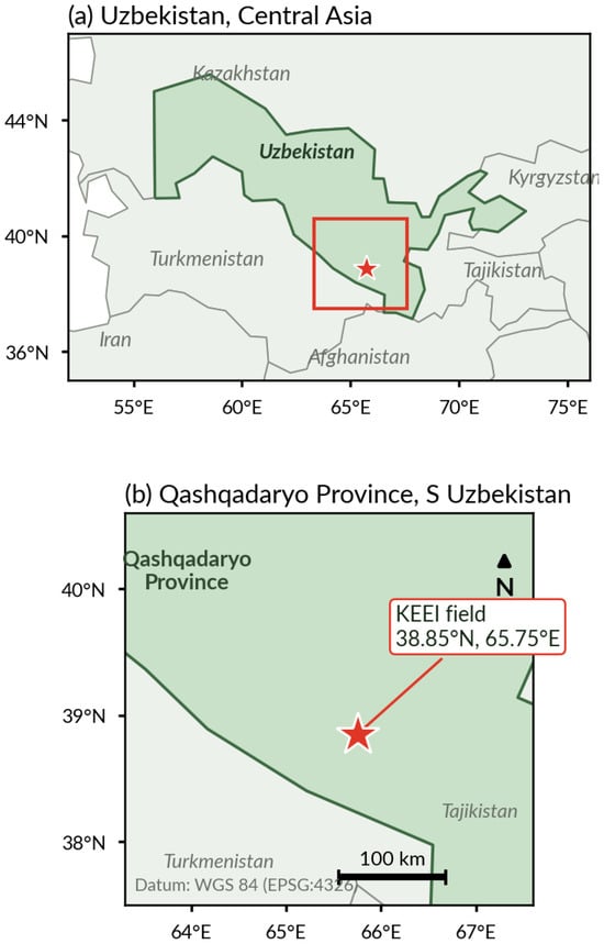
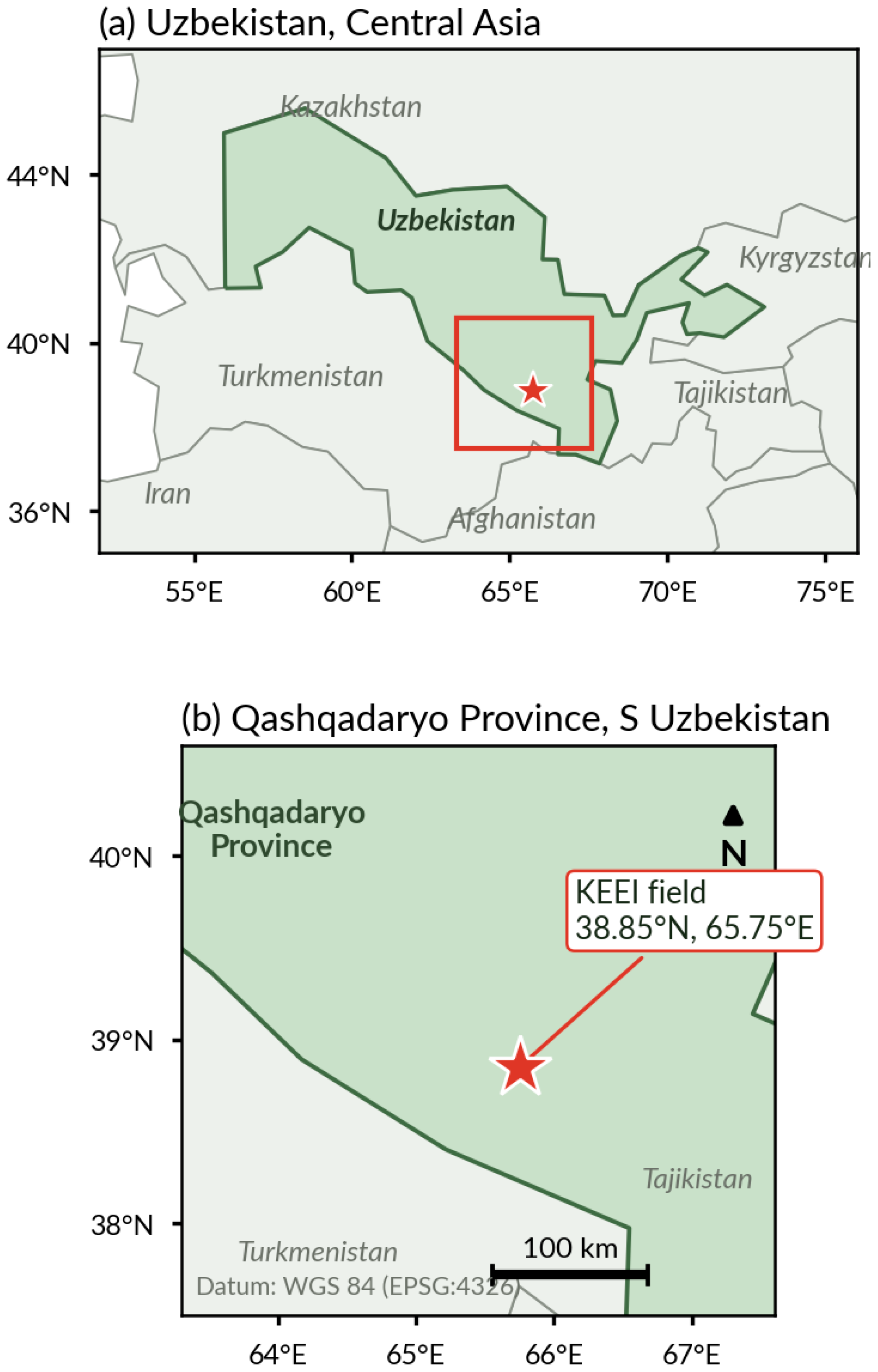
Field validation was conducted at the Karshi Engineering and Economics Institute (KEEI) experimental field near Karshi, Qashqadaryo province, Uzbekistan (approximate coordinates 38.85° N, 65.75° E). The coordinates are approximate and should not be interpreted as GPS-surveyed plot boundaries. The site represents an irrigated cotton-production context in Southern Uzbekistan, where continental-arid conditions, hot dry summers, and dependence on irrigation shape crop development and pest-management timing. Broader regional cotton-water and cotton-phenology literature provides background for this context, but the present field validation remains site-specific [16,17,18]. The regional setting of the experimental field and the location of the experimental field are shown in Figure 1.

Figure 1. Geographic location of the experimental field.

The experimental field has a continental, cold semi-arid climate (Köppen–Geiger class BSk) [19]. Long-term climate normals for the Karshi/Qashqadaryo area indicate a mean annual air temperature of approximately 16–17 °C, a hot and effectively rainless summer (mean July temperature near 30 °C, with daytime maxima frequently exceeding 35 °C) and cool winters (mean January temperature about 3 °C) [20]. Mean annual precipitation is low, on the order of 250–290 mm, and falls mainly between late autumn and early spring, so that the April–October cotton growing season depends almost entirely on irrigation. These continental-arid conditions—high summer evaporative demand, a long frost-free period and strong dependence on furrow irrigation from Amu Darya-derived water—shape crop development and the timing of plant-protection interventions in the Karshi/Qashqadaryo irrigated cotton system.

The field experiment used Bukhara-102, a medium-maturity Gossypium hirsutum cultivar. Sowing was conducted on 12–15 April 2023 and 8–10 April 2024. Row spacing was 60 cm, with a target final plant density of 85,000–95,000 plants/ha and final intra-row spacing after thinning and stand establishment of approximately 17.5–20.0 cm. Basal fertilizer consisted of 200 kg/ha NPK 10-20-20 before sowing, followed by 150 kg/ha urea split between SP2 and SP4.

The soil at the KEEI experimental field was recorded in field records as typical gray desert/sierozem soil with loam to medium-textured loam texture, pH 7.8–8.1, electrical conductivity 0.8–1.4 dS/m, and organic matter 0.9–1.2%. Irrigation was by furrow method using Amu Darya-derived irrigation water, with 8–10 irrigations per season and an approximate seasonal irrigation volume of 5500–6500 m³/ha. Year-specific weather summaries were not included as explanatory covariates; therefore, weather-related interpretation is restricted to the general continental-arid production context.

The agronomic sampling frame was therefore intentionally local: one irrigated KEEI/Karshi experimental context, one medium-maturity cultivar, and the Karshi/Qashqadaryo expert and image-contributor network.

2.2. Development of the Spraying Phase Scale

The Spraying Phase (SP) scale was developed through two consecutive moderated focus-group rounds with 16 expert panelists (senior cotton agronomists) representing the Karshi/Qashqadaryo production context. The panel included research-station specialists, extension or consultancy agronomists, and large-farm managers, each with more than ten years of practical crop-protection experience. The same 16 panelists also served as primary image contributors and primary labelers, but they were distinct from the three independent validation agronomists described below.

The first round elicited field-visible phenological markers and spray-timing rules used in practice. Candidate stages were proposed from repeated decision points described by the panelists. After the first round, structured notes were consolidated into draft phase definitions. The second round compared the draft stages, merged overlapping concepts, clarified ambiguous boundaries, and tested the definitions against field examples. For example, the SP3-SP4 boundary was anchored to the first visible buds, while mixed-stage scenes were assigned according to the dominant visible cue unless a decisive later-stage cue, such as open flowers or hardening bolls, was present.

Formal voting and a Delphi procedure were not used because the objective was to establish shared operational definitions through direct terminology calibration rather than to quantify anonymous preferences. Consensus was defined as the absence of unresolved substantive objections after discussion of boundary cases. If disagreement had remained unresolved, the affected boundary would have been retained for additional field review rather than forced by majority vote. Final definitions were circulated after the second round and confirmed in writing by the panelists.

2.3. Operational SP-Stage Definitions and Approximate BBCH Alignment

The final SP scale comprised six consecutive field-visible phases used as the reference standard for image labeling and spray-timing interpretation (Table 1).

Table 1. Operational spraying phase (SP) definitions and approximate BBCH alignment.

SP Stage	Operational Field Cue	Approximate BBCH Interval	Decision Relevance
SP1	Emergence of the first true leaf	09–11	Early establishment and early sap-sucking pest observation
SP2	Vegetative leaf growth and first lateral shoots	12–34	Canopy development and early pest scouting
SP3	Stem elongation and leaf closure	35–50	Canopy closure and changing spray penetration
SP4	First visible flower buds/squares	51–59	Bud-stage intervention window
SP5	First open flowers to mid-flowering	60–69	Flowering-stage protection window
SP6	Boll development until the first boll opening	70–80	Early boll protection and maturation window

2.4. Smartphone Image Dataset, Screening, and Labeling

Images were collected from April to October in 2023 and 2024 by the 16 expert panelists acting as primary contributors and primary labelers. The collection consisted of non-standardized smartphone images taken during routine fieldwork. Device models included Xiaomi Redmi Note 12 Pro (Xiaomi Corporation, Beijing, China), Samsung Galaxy A54 (Samsung Electronics Co., Ltd., Suwon-si, Republic of Korea), iPhone 13 (Apple Inc., Cupertino, CA, USA), and similar smartphones. Images were recorded as JPEG files; more than 95% of retained images had a resolution of at least 3000 × 4000 px, and the average file size was approximately 2.8 MB. This smartphone-only design was distinct from UAV/aerial cotton-imaging studies [21,22].

The initial image pool contained 14,887 smartphone images. Technical screening, visual interpretability screening, and deduplication removed 487 images (approximately 3.3%). Removed images included 312 duplicate or near-duplicate images and 175 images with severe blur, strong shadow, incorrect plant object, or insufficient interpretability. Blur/sharpness screening used the variance of the Laplacian; images with variance below 80 were flagged for severe blur and technical exclusion when visual interpretability was also inadequate. The final screened dataset contained 14,400 images.

Primary labels were assigned by the contributing expert panelists using the SP definitions in Table 1. The final class distribution was SP1: 2290; SP2: 2400; SP3: 2170; SP4: 2680; SP5: 2500; and SP6: 2360 images. The 70/20/10 split was implemented as a realized image-level target under the constraint of farm/contributor-wise non-overlap. Images from the same farm/contributor collection unit were not distributed across training, validation, and test subsets. The final split contained 10,080 training images, 2880 validation images, and 1440 test images.

The dataset included 16 farm/contributor collection units. The mean number of retained images per unit was 900, with a minimum, median, and maximum of 680, 905, and 1120 images, respectively. The largest contributor represented 7.8% of the final dataset, reducing the risk that a single farm/contributor dominated model evaluation.

The farm/contributor-wise split was used as both a leakage-control and environmental-bias mitigation step. Deduplication and near-duplicate removal were completed before final partitioning so that visually similar images could not inflate held-out performance across subsets. Images from the same farm/contributor collection unit were confined to a single partition, which reduced the possibility that the test set measured memorization of the same field background, soil color, irrigation geometry, or contributor-specific image style. This procedure reduces, but does not eliminate, environmental background bias because all collection units came from the same Karshi/Qashqadaryo production context.

Device model, JPEG compression, illumination, and viewpoint variability were treated as part of real-field image acquisition rather than as fully controlled experimental factors. Complete stage-wise distributions of device model, exposure, illumination category, and camera angle were not available; therefore, robustness across these factors was evaluated indirectly through contributor-wise hold-out testing and is treated as a transferability limitation.

2.5. Independent SP-Label Validation

A separate panel of three independent validation agronomists was used to evaluate SP-label consistency. These validators were not involved in SP-scale development, primary image collection, or primary labeling. They are referred to as Validator A (university agronomist, 18 years of experience), Validator B (plant-protection specialist), and Validator C (senior large-scale farm agronomy consultant, 22 years of experience).

The validation subset contained 300 images, stratified at approximately 50 images per SP class. Images were presented in randomized order under blinded conditions. No CNN predictions, dates, farm identifiers, or metadata were shown, and validators used only the written SP-stage definitions. Each validator assigned one SP label to each image. Inter-rater agreement was quantified with pairwise Cohen’s kappa. Disagreements were resolved through criteria-based adjudication anchored to the written SP definitions and the dominant visible phenological cue.

Pairwise Cohen’s kappa values were 0.83, 0.87, and 0.85, giving a mean kappa of 0.85. Twenty-seven of 300 images (9.0%) required adjudication. Disagreements were concentrated mainly at transitional boundaries: 12 cases at SP3-SP4, 9 cases at SP5-SP6, and 6 cases at other boundaries.

SP labels were treated as expert-derived operational reference labels rather than direct physiological ground truth. The independent validation step was therefore used to quantify label consistency and to identify boundary regions where subjective interpretation could affect model training. The concentration of adjudicated cases at SP3-SP4 and SP5-SP6 was consistent with gradual phenological transitions rather than random label instability.

2.6. CNN Training and Evaluation

A ResNet-50 convolutional neural network pretrained on ImageNet was fine-tuned to classify the six SP stages. The final classification layer was replaced with a six-class output head corresponding to SP1–SP6. All images were resized to 512 × 512 px, converted to RGB if necessary, normalized, and processed using the screened train/validation/test partitions described above. Smartphone-image screening and preprocessing, CNN fine-tuning, SP-label agreement analysis, and model-evaluation metric calculation were implemented in Python (v3.12.12) using PyTorch (v2.12.1), torchvision (v0.27.1), OpenCV-Python (v4.13.0.92), and scikit-learn (v1.9.0).

Training used the Adam (adaptive moment estimation) optimizer with an initial learning rate of 1 × 10⁻⁴, batch size of 16, dropout of 0.3 in the classifier head, and early stopping based on validation loss. Conservative augmentation was applied only to the training set and included random horizontal and vertical flips, rotations of ±10°, and mild brightness/contrast jitter. Model performance was evaluated on the held-out SP-label test set using accuracy, macro F1-score, precision, recall, and class-wise support.

Augmentation was intentionally conservative to avoid generating visually implausible phenological cues. The resulting performance should therefore be interpreted as SP-stage classification under the screened contributor-wise test design, not as evidence that all possible device, illumination, viewpoint, and canopy-architecture conditions have been simulated.

2.7. SP-BBCH Alignment and Interpretation Boundary

The SP scale was aligned conceptually with BBCH stages to support interpretation against an established phenological framework. Each SP stage was mapped to an approximate BBCH interval using the field-visible boundary points in Table 1. This alignment was used to compare decision windows, not as a direct BBCH-level CNN validation.

Consequently, the CNN result should not be interpreted as BBCH-stage recognition. The image model evaluated recognition of the locally defined SP scale, whereas the field comparison evaluated SP-guided timing against BBCH-based timing under matched spray protocols. Direct SP-to-BBCH tool comparison at the image-classification level requires image-level CNN predictions linked to BBCH labels and remains future work.

2.8. Field-Validation Design and Spray Protocol

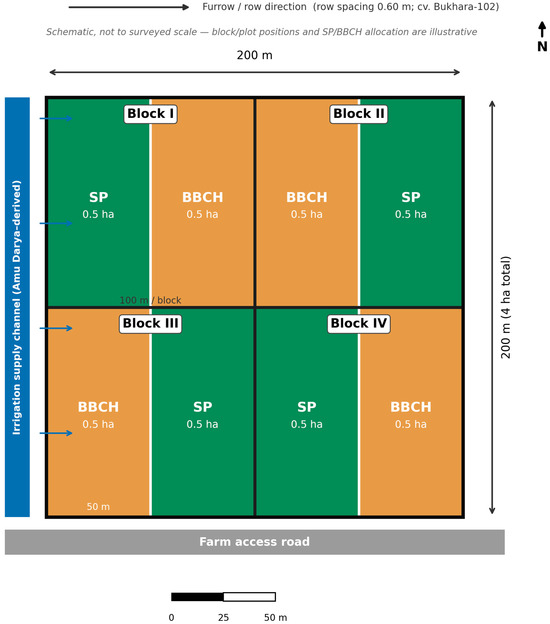
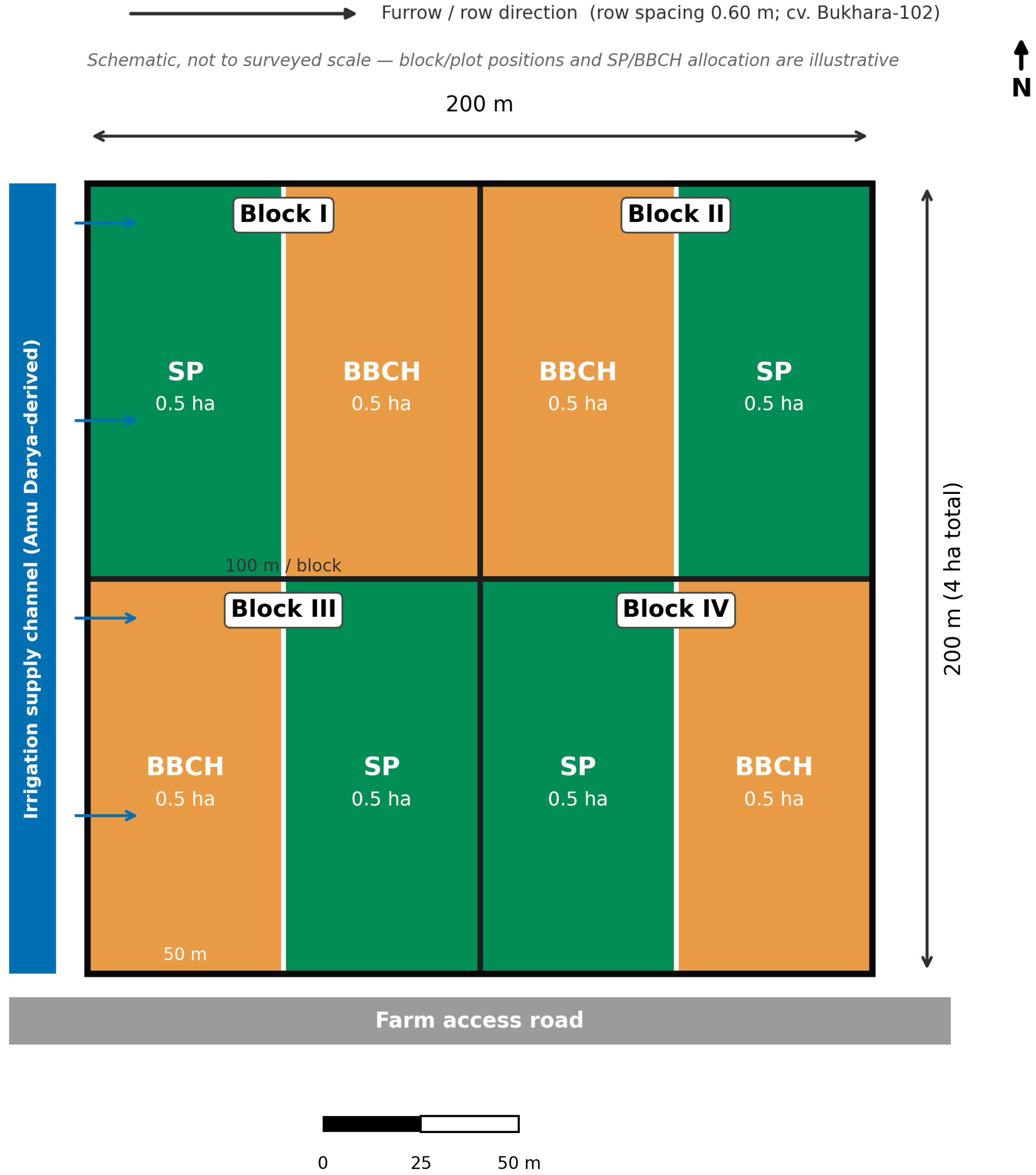
Field validation used a 4-ha experimental block at the KEEI experimental field over the 2023 and 2024 seasons. The design was an internally controlled timing comparison framed as an RCBD-style paired field validation (Figure 2 and Table 2).

Figure 2. Representative schematic of the 4-ha field-validation layout. Note: The area comprising four ≈1-ha blocks, each divided into two adjacent ≈0.5-ha plots assigned to SP-based and BBCH-based spray timing (RCBD-style paired design), with furrow irrigation from an Amu Darya-derived supply channel and cotton rows at 0.60 m spacing (cv. Bukhara-102). The schematic is illustrative and not to survey scale; block, plot and treatment positions do not depict the exact in-field randomization. Blocks I–IV denote the four RCBD-style field-validation blocks; each block contained one SP-based timing plot and one BBCH-based timing plot.

Table 2. Field-validation setup.

Item	Description
Location	KEEI experimental field, near Karshi, Qashqadaryo province, Uzbekistan
Approximate coordinates	38.85° N, 65.75° E
Experimental area	4 ha
Blocks	Four approximately 1-ha blocks
Plot arrangement	Two adjacent approximately 0.5-ha plots per block
Treatments	SP-based timing vs. BBCH-based timing
Seasons	2023 and 2024
Replication	8 block-year replicates
Controlled factors	cultivar, planting density, fertilization, irrigation, product set, per-application dose, sprayer, nozzle configuration, operator, and plot management
Variable factor	spray-timing strategy

The same AMAZONE UF 2001 rear-mounted field sprayer (AMAZONE Technologie GmbH & Co. KG, Bramsche, Germany) was used for all applications. The sprayer had an 18 m boom with 36 Lechler ID 120° air-inclusion flat-fan anti-drift nozzles (Lechler GmbH, Metzingen, Germany) at 50 cm spacing. The exact nozzle size code was not recorded. Spray pressure was 3.0–3.5 bar, water volume was 250 L/ha, and travel speed was 6.5 km/h. Product doses were diluted in the standard 250 L/ha spray volume. Before each application, calibration included nozzle-discharge checking, pressure-stability checking, and travel-speed checking.

The same trained operator performed all applications across both treatments and both seasons. Controlled factors included sprayer, nozzle configuration, operator, water volume, pressure range, travel speed, product set, per-application product dose, cultivar, fertilization, irrigation, and plot management. Treatments differed only in spray-timing strategy and the resulting application frequency.

Products, per-application doses, timing windows, and targets are summarized in Table 3a,b.

Table 3. (a) Plant-protection products and per-application doses used in both treatments. (b) Timing windows and main target groups for the plant-protection products.

(a)
Product	Active Ingredient	Product Dose	Active-Ingredient Dose
Actara 240 SC	thiamethoxam	0.15 L/ha	36 g a.i./ha
Karate Zeon	lambda-cyhalothrin	0.50 L/ha	50 g a.i./ha
Proclaim	emamectin-benzoate	0.40 kg/ha	8 g a.i./ha
Ampligo	chlorantraniliprole + lambda-cyhalothrin	0.30 L/ha	30 + 15 g a.i./ha
(b)
Treatment	Timing Window	Product	Main Target
Both	SP1/corresponding early BBCH stage	Actara 240 SC	thrips, aphids
Both	SP3-SP4/BBCH 35–51	Karate Zeon	lepidopteran larvae
Both	SP4-SP5/BBCH 51–60	Proclaim	bollworm
Both	SP5-SP6/BBCH 60–70	Ampligo	bollworm, aphids

Note: The product set and per-application product doses were identical in both treatments. Seasonal active-ingredient totals are not reported because a product-specific seasonal active-ingredient-total table was not retained in a publication-ready form. The retained plot-level ERI outcome was analyzed as the environmental risk endpoint.

2.9. Yield Determination and Lint-Equivalent Yield Estimation

At harvest, cotton from the harvestable area of each plot was recorded separately by year, block, treatment, and harvest event. Where more than one picking was conducted, plot-level harvest records were summed before yield calculation. Plot-level seed-cotton yield was first calculated from harvested seed-cotton mass and harvested plot area. Because complete plot-specific ginning turnout was not available for all plots, lint-equivalent yield was calculated using the retained KEEI harvest records and the available KEEI ginning documentation at the treatment-year or aggregate record level. The resulting values should therefore be interpreted as plot-level lint-equivalent yield estimates. Because the absolute lint-equivalent yield level reflects high-yield irrigated experimental plots, it should be interpreted as a KEEI/Karshi field-validation outcome rather than as a regional or national production average.

2.10. Environmental Risk Index (EIQ/ERI), Statistical Analysis, and Economic Interpretation

Environmental risk was quantified using the Cornell Environmental Impact Quotient (EIQ) field-use approach and the versioned Cornell IPM EIQ active-ingredient database [23]. For each application, field-use EIQ was calculated for each active ingredient and summed across applications to obtain a plot-level Environmental Risk Index (ERI). Equations (1) and (2) define the calculation structure.

$$EI{Q}_{FUR,i,k}=EI{Q}_i\times R_{i,k}^{a.i}$$

(1)

$$ERI={\mathit{\Sigma }}_{i=1}^n{\mathit{\Sigma }}_{k=1}^{m_i}EI{Q}_{FUR,i,k}$$

(2)

In Equation (1), $EI{Q}_{FUR,i,k}$ is the field-use EIQ value for active ingredient i in application k; $EI{Q}_i$ is the published Environmental Impact Quotient for active ingredient i; and $R_{i,k}^{a.i}$ is the active-ingredient application rate for active ingredient i in application k. In Equation (2), n is the number of active ingredients, m_i is the number of applications for active ingredient i, and ERI is the plot-level seasonal sum of field-use EIQ values. EIQ and ERI are unitless comparative indices. Because $R_{i,k}^{a.i}$ is already defined as an active-ingredient application rate, Equation (1) does not include an additional active-ingredient fraction multiplier.

Field outcomes were analyzed across eight block-year replicates. Treatment effects for cost, lint-equivalent yield, and ERI were evaluated using the reported RCBD-style model outputs, with treatment as the main fixed effect and block-year replication used for field-validation inference. Application frequency is reported descriptively because product-specific replicate-level application counts were not available for a separate inferential test. RCBD-style inferential analyses for crop-protection cost, plot-level lint-equivalent yield, and ERI were performed in R (v4.6.1; R Foundation for Statistical Computing, Vienna, Austria) using the base stats package included with R.

Economic interpretation used a local farm-gate lint cotton price of 1850 USD/t from local procurement records. The partial-budget interpretation combined additional gross lint-equivalent value with crop-protection cost savings. This calculation represents a partial-budget advantage before additional implementation, advisory, or digital-deployment costs and should not be interpreted as a complete profit estimate.

3. Results

The two-round expert process produced six operational SP stages anchored to field-visible cues (Table 1). The final definitions were accepted through written confirmation after boundary-case discussion. Results are reported without repeating the full operational definitions already given in Section 2.3.

Technical screening reduced the initial 14,887-image pool to 14,400 retained smartphone images. The exclusion of 487 images (approximately 3.3%) was mainly due to duplicates, near-duplicates, severe blur, strong shadow, incorrect plant object, or insufficient interpretability. The final dataset maintained broad SP-stage representation and avoided dominance by a single farm/contributor collection unit.

Independent SP-label validation showed high inter-rater agreement. Pairwise Cohen’s kappa values ranged from 0.83 to 0.87, with a mean of 0.85. Adjudication was required for 27 images (9.0%), primarily at SP3-SP4 and SP5-SP6 boundaries, consistent with gradual phenological transitions.

3.1. CNN SP-Stage Classification

The CNN achieved 93.0% overall accuracy on the held-out SP-label test set (n = 1440). Class-wise metrics were high across all six SP classes, and residual errors were concentrated mainly between adjacent stages (Table 4).

Table 4. CNN performance metrics for SP1–SP6 classification on the held-out test set (n = 1440).

SP Class	Precision (%)	Recall (%)	F1-Score (%)	Support (n)
SP1	95.0	94.0	94.6	229
SP2	94.0	97.0	95.5	240
SP3	96.0	90.0	92.9	217
SP4	97.0	92.0	94.4	268
SP5	93.0	95.0	94.0	250
SP6	92.0	91.0	91.5	236
Total/average	94.5	93.2	93.8	1440

The SP-BBCH alignment remained a phenological interpretation tool rather than a BBCH-level CNN validation. Direct BBCH-level confusion metrics were not calculated because image-level CNN predictions linked to BBCH labels were not available in the revision dataset.

These metrics evaluate SP-stage classification on held-out farm/contributor units. They should therefore be read as an internal contributor-wise validation of the SP-label recognition task, not as external validation across other Uzbek provinces, cultivars, device distributions, or BBCH categories. Accordingly, no BBCH-stage classification accuracy, BBCH-level precision, recall, F1-score, or BBCH confusion matrix is reported or claimed in this study.

3.2. Field-Validation Outcomes

Yield values reported in Table 5 and Table 6 represent plot-level lint-equivalent yield estimates, not seed-cotton field weight and not directly measured recovered lint mass for every plot. SP-guided scheduling showed a descriptive reduction in the mean number of pesticide applications from 4.88 to 3.75 applications per season, corresponding to a 23.1% reduction in application frequency relative to BBCH-based scheduling. The same product set and per-application product doses were used in both treatments; therefore, the observed difference reflects timing strategy and resulting application frequency rather than a change in product selection or per-application dose. Table 5 provides a concise descriptive overview of the field-validation outcomes for SP-guided and BBCH-based timing, including mean application frequency, crop-protection cost, plot-level lint-equivalent yield, ERI, and the corresponding relative changes. Application frequency is presented descriptively, whereas crop-protection cost, plot-level lint-equivalent yield, and ERI were evaluated inferentially.

Table 5. Average plot-level outcomes comparing SP-guided and BBCH-based timing in the 4-ha field validation.

Metric	SP Timing	BBCH Timing	Relative Change
Mean pesticide applications per season	3.75	4.88	−23.1%
Crop-protection cost (USD/ha)	113.38	143.88	−21.2%
Plot-level lint-equivalent yield (t/ha)	3.56	3.40	+4.5%
Environmental risk index	0.66	0.84	−21.6%

Note: Application frequency is descriptive. Cost, plot-level lint-equivalent yield, and ERI values are field-validation outcomes; ERI = Environmental Risk Index. Relative changes were calculated from unrounded values; displayed means are rounded for readability.

Table 6. RCBD-style summary statistics for cost, plot-level lint-equivalent yield, and ERI.

Metric	SP Mean ± SD (SE; 95% CI)	BBCH Mean ± SD (SE; 95% CI)	Delta (95% CI)	p
Cost (USD/ha)	113.38 ± 9.84 (3.48; 105.15–121.60)	143.88 ± 12.44 (4.40; 133.48–154.27)	−30.50 (−44.97; −16.03)	0.0016
Plot-level lint-equivalent yield (t/ha)	3.56 ± 0.20 (0.07; 3.39–3.72)	3.40 ± 0.14 (0.05; 3.29–3.52)	+0.154 (+0.084; +0.223)	0.0012
Environmental risk index	0.66 ± 0.07 (0.03; 0.59–0.72)	0.84 ± 0.05 (0.02; 0.79–0.88)	−0.180 (−0.259; −0.101)	0.0010

For clarity, the term plot-level lint-equivalent yield in Table 5 and Table 6 denotes yield calculated from plot-level seed-cotton harvest records and the available KEEI harvest/ginning documentation. It is not the field weight of seed cotton and should not be interpreted as directly measured recovered lint mass for every plot. Because complete plot-specific ginning turnout was not available for all plots, the values should be interpreted as lint-equivalent plot-level yield estimates under the controlled irrigated KEEI/Karshi experimental conditions.

Reported RCBD-style model outputs showed significant treatment effects for crop-protection cost (F(1,7) = 24.83, p = 0.0016), lint-equivalent yield (F(1,7) = 27.36, p = 0.0012), and ERI (F(1,7) = 28.98, p = 0.0010). The lint-equivalent yield difference was +0.154 t/ha (95% CI +0.084 to +0.223 t/ha). Based on F(1,7) = 27.36, the partial eta squared for lint-equivalent yield was 0.796, indicating a large treatment effect within this field-validation dataset. Table 6 presents the corresponding RCBD-style inferential summary for crop-protection cost, plot-level lint-equivalent yield, and ERI, including treatment means, standard deviations, standard errors, 95% confidence intervals, between-treatment differences, and p values.

At a local farm-gate lint cotton price of 1850 USD/t, the observed lint-equivalent yield advantage corresponded to approximately 285 USD/ha in additional gross lint-equivalent value. Combined with the reported crop-protection cost saving of 30.5 USD/ha, this implies a partial-budget advantage of approximately 315 USD/ha before accounting for any additional implementation, advisory, or digital-deployment costs. This value should not be interpreted as a complete profit estimate.

4. Discussion

The field validation indicates that SP-based timing can improve crop-protection efficiency under the tested Karshi/Qashqadaryo irrigated cotton conditions. The key agronomic effect was not a change in product choice or per-application dose, but a reduction in application frequency while maintaining the same product set and spray protocol. This distinction is important because it isolates timing as the main management factor evaluated in the field comparison.

The reductions in crop-protection cost and ERI are consistent with the lower application frequency. Because ERI was calculated from EIQ field-use values, it should be interpreted as comparative risk potential rather than a direct measurement of ecological impact. The field validation nevertheless suggests that better temporal alignment between crop stage and intervention window can reduce unnecessary applications and lower relative environmental risk under otherwise matched conditions.

The observed lint-equivalent yield increase was modest in relative terms but statistically and economically meaningful within the field-validation dataset. The partial eta squared for lint-equivalent yield was 0.796, and the yield difference translated into approximately 285 USD/ha in additional gross lint-equivalent value at the local farm-gate lint cotton price used for the partial-budget calculation. This interpretation remains partial because implementation, training, advisory, and digital-deployment costs were not included.

The absolute lint-equivalent yield level observed in both treatments is high and should not be generalized to average Uzbek cotton production. The comparison is internally interpretable as a paired field-validation contrast because the same harvest-record and lint-equivalent conversion procedure was applied in both treatments, and because cultivar, planting density, irrigation, fertilization, product set, per-application dose, sprayer, nozzle configuration, operator, and plot management were held constant. However, because complete plot-specific ginning turnout was not available for all plots, the absolute lint-equivalent values should be interpreted cautiously. The practical interpretation should focus primarily on the within-experiment treatment difference (+0.154 t/ha) and the associated partial-budget calculation rather than on extrapolating the absolute yield level to broader regions.

4.1. CNN-Based SP Recognition, Bias Control, and Decision-Support Feasibility

Several potential sources of model bias remain relevant when interpreting the CNN result. Contributor-wise splitting and duplicate removal reduced leakage from near-identical images and limited farm-specific background memorization, but they do not prove robustness to other provinces, cultivars, soil backgrounds, irrigation layouts, camera pipelines, or lighting regimes. The 93.0% test accuracy should therefore be interpreted as performance on held-out SP-labeled contributor units within the Karshi/Qashqadaryo sampling frame.

Device and illumination bias are also possible because smartphone models differ in sensor properties, automatic white balance, sharpening, compression, and color rendering. Similarly, outdoor illumination, shadows, dust, canopy density, and viewpoint may affect the visibility of buds, flowers, and bolls. Future model evaluation should therefore include device-stratified and illumination-stratified tests, stronger color normalization, random cropping, viewpoint perturbation, and domain-adaptation experiments.

The CNN results show that the expert-defined SP stages were visually learnable from non-standardized smartphone images collected under routine field conditions. The 93.0% test accuracy and high class-wise F1-scores indicate that canopy, bud, flowering, and early boll cues were sufficiently distinctive for SP-stage classification. The validation result should be interpreted specifically as SP-label classification, not as direct BBCH-level CNN validation.

The dataset-screening information adds practical context to the model results. Most retained images had high native smartphone resolution, but acquisition conditions were not standardized. Screening removed only a small proportion of images, including severe blur and uninterpretable cases. These robustness issues should be addressed in future external validation. The present study supports the feasibility of SP recognition, but it does not validate a complete on-device advisory system. Practical deployment would require offline image capture or delayed upload where network coverage is inconsistent, model compression or server-side inference depending on device capacity, user-interface testing, extension-worker training, feedback mechanisms, implementation-cost assessment, and local responsibility rules for advisory recommendations.

4.2. Comparison with BBCH-Based and Other Timing Approaches

The BBCH framework remains valuable for standardized phenological communication, but the SP scale was designed for local spray-timing decisions. The SP-BBCH alignment, therefore, should be read as a conceptual bridge between an operational local scale and an international descriptive scale. Direct tool comparison at the CNN level will require image-level predictions linked to BBCH labels so that mapped confusion metrics can be calculated.

The present field comparison, therefore, evaluates two timing logics under matched agronomic and spray-management conditions; it should not be read as a direct image-classifier comparison between SP and BBCH.

Comparisons with threshold-based spraying in Mali, sensor-guided application in Brazil, and growth-stage-based disease management in rice support the broader principle that interventions are more efficient when aligned with biological need [24,25,26,27,28,29,30,31]. However, the transferability of just-in-time application depends on the cropping system, pest complex, irrigation regime, climate, cultivar maturity, farm size, pesticide regulation, and extension support. The current results should therefore be treated as evidence from one irrigated cotton context rather than proof of broader geographic performance.

4.3. Limitations, Transferability, and Future Research

Several limitations define the interpretation of this study. Field validation was conducted at a single KEEI/Karshi site over two seasons using one medium-maturity cultivar and one locally defined expert and image-contributor network. The results, therefore, support internal validity within the tested Karshi/Qashqadaryo irrigated cotton context, but they do not establish national representativeness. The image dataset reduced leakage through contributor-wise splitting and duplicate screening, but external robustness to other provinces, cultivars, farm backgrounds, device pipelines, lighting conditions, and canopy architectures remains untested. CNN performance was evaluated against SP labels; direct BBCH-level CNN consistency and confusion analysis were not available for this revision. Similarly, the study did not include device-stratified or illumination-stratified external validation, complete brightness/exposure distributions, on-device deployment testing, or a complete profit analysis. The spray protocol was described from available field records, but the exact nozzle size code and some formulation-label details were not available beyond the recorded product and active-ingredient rates. Seasonal active-ingredient totals were not reported because product-specific seasonal application counts were not retained in publication-ready form. Finally, the reported yield values represent plot-level lint-equivalent yield estimates derived from plot-level harvest records and the available KEEI harvest/ginning documentation; they should therefore be interpreted together with the high-yield irrigated experimental context and not generalized as directly measured plot-level lint yield or as a regional production average.

Future work should validate the SP scale across additional farms, provinces, cultivars, pest-pressure regimes, and seasons. It should also test dose adjustment, alternative active ingredients, biological control integration, resistance-management strategies, and direct comparison of SP- and BBCH-level CNN predictions.

5. Conclusions

This study developed and evaluated an expert-defined SP scale for cotton spray-timing support under Karshi/Qashqadaryo irrigated production conditions. The CNN model classified SP stages from screened smartphone images with 93.0% test accuracy under a contributor-wise validation design, and SP-guided field scheduling reduced application frequency, crop-protection cost, and ERI while modestly increasing plot-level lint-equivalent yield relative to BBCH-based timing. The findings support SP-guided timing as a locally calibrated decision-support concept with internal validity under the tested KEEI/Karshi conditions, but not as proof of national-scale performance or operational deployment readiness. Multi-site, multi-cultivar, multi-season, device-stratified, illumination-stratified, and BBCH-level validation, together with harvest/ginning transparency and implementation-cost assessment, is required before broader recommendations are made.

References

- US Department of Agriculture, Foreign Agricultural Service. Cotton: World Markets and Trade; US Department of Agriculture: Washington, DC, USA, 2026. Available online: https://apps.fas.usda.gov/psdonline/circulars/cotton.pdf (accessed on 20 March 2026).
- US Department of Agriculture, Foreign Agricultural Service. Cotton and Products Annual—Republic of Uzbekistan; Report No. UZ2024-0001; Tashkent, Uzbekistan. 2024. Available online: https://apps.fas.usda.gov/newgainapi/api/Report/DownloadReportByFileName?fileName=Cotton%20and%20Products%20Annual_Tashkent_Uzbekistan%20-%20Republic%20of_UZ2024-0001.pdf (accessed on 21 March 2026).
- Khor, L.Y.; Feike, T. Economic sustainability of irrigation practices in arid cotton production. Water Resour. Econ. 2017, 20, 40–52. [Google Scholar] [CrossRef] [Scilit]
- Kavi, P.I.; Amarnath, J.S.; Sivasankari, B. Economic and environmental impact of pesticide use in conventional cotton and bt cotton. Econ. Aff. 2018, 63, 425–431. [Google Scholar] [CrossRef] [Scilit]
- Shokirova, G.; Juraev, Z. Combating the devastating effects of cotton bollworm: Case of Uzbekistan. F1000Research 2024, 13, 39. [Google Scholar] [CrossRef] [Scilit]
- Mathari, J.R.J.; Mohideen, H.S. Cotton (Gossypium spp.) pest management in the era of next-generation sequencing: A review. J. Appl. Biol. Biotechnol. 2023, 11, 10–17. [Google Scholar] [CrossRef] [Scilit]
- Munger, P.; Bleiholder, H.; Hack, H.; Hess, M.; Stauss, R.; Van den Boom, T.; Weber, E. Phenological growth stages of the cotton plant (Gossypium hirsutum L.): Codification and description according to the BBCH scale. J. Agron. Crop Sci. 1998, 180, 143–149. [Google Scholar] [CrossRef] [Scilit]
- Meier, U. Growth Stages of Mono- and Dicotyledonous Plants—BBCH Monograph; Julius Kühn-Institut (JKI): Quedlinburg, Germany, 2018. [Google Scholar]
- Reeb, R.A.; Aziz, N.; Lapp, S.M.; Kitzes, J.; Heberling, J.M.; Kuebbing, S.E. Using convolutional neural networks to efficiently extract immense phenological data from community science images. Front. Plant Sci. 2022, 12, 787407. [Google Scholar] [CrossRef] [Scilit] [PubMed]
- Coleman, G.R.; Kutugata, M.; Walsh, M.J.; Bagavathiannan, M.V. Multi-growth stage plant recognition: A case study of Palmer amaranth (Amaranthus palmeri) in cotton (Gossypium hirsutum). Comput. Electron. Agric. 2024, 217, 108622. [Google Scholar] [CrossRef] [Scilit]
- Yalcin, H. Plant phenology recognition using deep learning: Deep-Pheno. In Proceedings of the 2017 6th International Conference on Agro-Geoinformatics, Fairfax, VA, USA, 7–10 August 2017; pp. 1–5. [Google Scholar]
- Qin, J.; Hu, T.; Yuan, J.; Liu, Q.; Wang, W.; Liu, J.; Guo, L.; Song, G. Deep-learning-based rice phenological stage recognition. Remote Sens. 2023, 15, 2891. [Google Scholar]
- Schieck, M.; Krajsic, P.; Loos, F.; Hussein, A.; Franczyk, B.; Kozierkiewicz, A.; Pietranik, M. Comparison of deep learning methods for grapevine growth stage recognition. Comput. Electron. Agric. 2023, 211, 107944. [Google Scholar] [CrossRef] [Scilit]
- Yang, H.-C.; Zhou, J.-P.; Zheng, C.; Wu, Z.; Li, Y.; Li, L.-G. PhenologyNet: A fine-grained approach for crop-phenology classification fusing convolutional neural network and phenotypic similarity. Comput. Electron. Agric. 2025, 229, 109728. [Google Scholar]
- Puelles, M.; Arbizu-Milagro, J.; Castillo-Ruiz, F.J.; Peña, J.M. Predictive models for grape downy mildew (Plasmopara viticola) as a decision support system in Mediterranean conditions. Crop Prot. 2024, 175, 106450. [Google Scholar]
- Abdullaev, I.; Giordano, M.; Rasulov, A. Cotton in Uzbekistan: Water and Welfare. In The Cotton Sector in Central Asia; Kandiyoti, D., Ed.; SOAS, University of London: London, UK, 2007; pp. 102–118. [Google Scholar]
- Tsiros, E.; Domenikiotis, C.; Dalezios, N.R. Assessment of cotton phenological stages using agroclimatic indices: An innovative approach. Ital. J. Agrometeorol. 2009, 1, 50–55. [Google Scholar]
- Gillham, F.E. Cotton Production Prospects for the Next Decade; World Bank Publications: Washington, DC, USA, 1995; Volume 23. [Google Scholar]
- Beck, H.E.; Zimmermann, N.E.; McVicar, T.R.; Vergopolan, N.; Berg, A.; Wood, E.F. Present and future Köppen-Geiger climate classification maps at 1-km resolution. Sci. Data 2018, 5, 180214. [Google Scholar] [CrossRef] [Scilit]
- Climate-Data.org. Qarshi Climate (Qashqadaryo, Uzbekistan): Climate Table and Graph. 2025. Available online: https://en.climate-data.org/asia/uzbekistan/qashqadaryo-province/qarshi-2777/ (accessed on 11 June 2026).
- Petti, D.; Li, C. Weakly-supervised learning to automatically count cotton flowers from aerial imagery. Comput. Electron. Agric. 2022, 194, 106734. [Google Scholar] [CrossRef] [Scilit]
- Khujamatov, H.; Muksimova, S.; Abdullaev, M.; Cho, J.; Lee, C.; Jeon, H.-S. Empowering smallholder farmers with UAV-based early cotton disease detection using AI. Drones 2025, 9, 385. [Google Scholar] [CrossRef] [Scilit]
- Cornell Integrated Pest Management. Environmental Impact Quotient Active Ingredient Database, Version 2026.02.12.1; Cornell University: Ithaca, NY, USA, 2026; Available online: https://eiq.cornell-ipm.org/about/data/ (accessed on 17 March 2026).
- Leach, A.; Gómez Santos, A.A.; Kaplan, I. Threshold-based management reduces insecticide use by 44% without compromising pest control or crop yield. Commun. Earth Environ. 2025, 6, 710. [Google Scholar] [CrossRef] [Scilit]
- Silvie, P.; Deguine, J.P.; Nibouche, S.; Michel, B.; Vaissayre, M. Potential of threshold-based interventions for cotton pest control by small farmers in West Africa. Crop Prot. 2001, 20, 297–301. [Google Scholar] [CrossRef] [Scilit]
- Settle, W.; Soumaré, M.; Sarr, M.; Garba, M.H.; Poisot, A. Reducing pesticide risks to farming communities: Cotton farmer field schools in Mali. Philos. Trans. R. Soc. B 2014, 369, 20120277. [Google Scholar] [CrossRef] [Scilit]
- Wang, S.; Li, Y.; Yuan, J.; Song, L.; Liu, X.; Liu, X. Recognition of cotton growth period for precise spraying based on convolution neural network. Inf. Process. Agric. 2021, 8, 219–231. [Google Scholar] [CrossRef] [Scilit]
- Abdullah, H.M.; Islam, M.; Islam, M.S.; Sen, S.; Tuhin, A.K.; Arman, S.E.; Hasan, M.M. Cotton seedling monitoring and growth stage classification integrating deep learning and feature engineering. Smart Agric. Technol. 2025, 12, 101619. [Google Scholar] [CrossRef] [Scilit]
- Zhang, X.; Chen, L. Bud YOLO: A real-time accurate detection method of cotton top buds in cotton fields. Agriculture 2024, 14, 1651. [Google Scholar] [CrossRef] [Scilit]
- Zanin, A.R.A.; Neves, D.C.; Teodoro, L.P.R.; da Silva Júnior, C.A.; da Silva, S.P.; Teodoro, P.E.; Baio, F.H.R. Reduction of pesticide application via real-time precision spraying. Sci. Rep. 2022, 12, 5638. [Google Scholar] [CrossRef] [Scilit] [PubMed]
- Xuan, T.H.; Gergon, E.B. Strategies for the management of rice pathogenic fungi. In Fungi; CRC Press: Boca Raton, FL, USA, 2018; pp. 396–431. [Google Scholar]
Disclaimer/Publisher’s Note: The statements, opinions and data contained in all publications are solely those of the individual author(s) and contributor(s) and not of MDPI and/or the editor(s). MDPI and/or the editor(s) disclaim responsibility for any injury to people or property resulting from any ideas, methods, instructions or products referred to in the content. |
© 2026 by the authors. Licensee MDPI, Basel, Switzerland. This article is an open access article distributed under the terms and conditions of the Creative Commons Attribution (CC BY) license.