


Abstract
Solar insecticidal lamps are important physical control devices for green pest management, but faults in their photovoltaic power supply units can reduce trapping efficiency and shorten service life. To improve fault identification under complex agricultural environments, this study proposes a signal-image-level multimodal fusion network (SIL-MMFN) for detecting and classifying photovoltaic panel operating states in solar insecticidal lamps. The method combines time-series measurements with short-time Fourier transform (STFT)-based time–frequency images. A convolutional image branch extracts spatial features from time–frequency representations, whereas a bidirectional GRU branch with attention models temporal dependencies in the original signals. In addition, physics-informed features based on the illumination–current residual and output power are introduced to enhance discriminative fault information. Field data collected from four agricultural deployment nodes were used to classify normal, open-circuit, and mismatch states. Experimental results show that the proposed method achieved an accuracy of 97.5%, precision of 96.7%, recall of 97.8%, and macro-F1 score of 97.3%, outperforming single-modality and representative comparison models. The results indicate that multimodal fusion helps reduce confusion between open-circuit and mismatch faults and provides a potential approach for operating-state monitoring and maintenance of agricultural photovoltaic equipment. In this study, fault diagnosis refers to the detection and classification of photovoltaic panel operating states, including normal, open-circuit, and mismatch conditions.
1. Introduction
Pests and diseases have become major constraints on agricultural production and the stable achievement of high crop yields. Crop losses caused by pests have long been recognized as a serious threat to agricultural productivity and food supply [1]. Although conventional chemical pesticide control can suppress pest occurrence and spread to some extent, long-term and intensive use can lead to environmental pollution, pesticide residues, ecological imbalance, and resistance development [2]. In this context, environmentally friendly and sustainable green control technologies have received increasing attention and have become an important direction for integrated pest management in modern agriculture [3].
Against this background, solar insecticidal lamps, as typical physical trapping devices, have been widely used for green pest control in farmland because of their energy-saving characteristics, environmental friendliness, flexible deployment, and independence from external power supplies. Research on pest phototactic rhythm provides an important biological basis for the application of solar insecticidal lamps in field pest management [4]. Photovoltaic agriculture has also created new opportunities for combining renewable energy supply with intelligent phytoprotection systems [5]. Recent agrivoltaics research has further summarized global potential, technologies, crops, and policy frameworks for integrating agricultural production with solar energy [6]. Solar hydrogen pathways based on urban BIPV and rural agri-PV have also been reviewed as emerging options for linking solar energy and agricultural systems [7]. Such devices usually rely on the coordinated operation of photovoltaic panels, controllers, energy storage units, and IoT monitoring modules, and lightweight fault detection studies have shown that equipment stability is essential for reliable SIL-IoT operation [8]. A recently published SIL fault dataset further indicates that real agricultural deployment data may contain complex state changes and fault patterns [9]. In related intelligent agricultural applications, deep learning has been used for moth detection from pheromone trap images [10]. Transformer-based edge computing methods have also been used for cotton pest and disease detection [11]. Data fusion and model fusion digital twins have been proposed for pest management systems [12]. Agrivoltaic research shows that agricultural production and photovoltaic power generation can be coupled in large-scale PV farms [13]. Rice agriphotovoltaic experiments further demonstrate the need to evaluate crop productivity together with solar power output [14]. Attention-enhanced convolutional networks have also been applied to crop disease diagnosis, indicating the broader value of deep learning in agricultural perception tasks [15]. However, because these systems are exposed to high temperatures, high humidity, strong solar radiation, dust deposition, and biological contamination for long periods, solar insecticidal lamps are prone to multiple faults that reduce system efficiency and may even cause device failure.
In addition to physical trapping, pest condition perception is an important function of intelligent pest management systems associated with solar insecticidal lamps. For example, deep learning-based moth detection from pheromone trap images achieved a maximum mAP of 90.25% [10], Transformer-based edge computing methods have been used for cotton pest and disease detection [11], and data fusion and model fusion digital twins have been proposed for pest management systems [12]. These studies suggest that intelligent pest detection and monitoring may provide useful information for field pest warning and management decisions. However, for solar insecticidal lamps, the effectiveness of pest monitoring and trapping also depends on the stable night-time operation of the lamp system, which is directly constrained by the reliability of the photovoltaic power supply unit.
These studies suggest that photovoltaic technology is increasingly being embedded into agricultural and rural energy systems rather than being used solely as an independent power generation infrastructure. Solar-PV feasibility research in high-altitude regions has shown that PV farms can support a sustainable electricity supply where geography and energy security are closely linked [16]. Agri-PV studies in developing countries further emphasize that photovoltaic systems can contribute to the water–energy–food nexus by combining energy production with sustainable agricultural use [17]. In addition, phase-change-material-based PV and building energy studies highlight the importance of thermal management and energy efficiency enhancement in PV-integrated systems [18]. Together with recent reviews on BIPV and rural agri-PV pathways for solar hydrogen production [7], these studies show that reliable PV operation and monitoring are important for agri-PV-related applications. Therefore, the fault detection and classification of the photovoltaic subsystem in solar insecticidal lamps is relevant to the broader agri-PV context because it supports a stable renewable energy supply for field-deployed agricultural equipment.
The photovoltaic panel is a key component of the solar insecticidal lamp (SIL), and its operating condition directly determines the power supply capacity and stability of the system. A review of photovoltaic fault diagnosis methods shows that open-circuit faults, mismatch, shading, soiling, and module defects are important causes of abnormal PV operation [19]. IoT-based PV fault detection research further shows that embedded monitoring can support fault identification in practical PV arrays [20]. Deep learning analysis of thermal images has been used to detect faults in photovoltaic farms [21]. Infrared thermography combined with machine learning and deep learning has also been assessed for photovoltaic fault diagnosis [22]. CNN-based models have been shown to classify photovoltaic array faults from data-driven representations [23]. For example, controller damage affects power regulation and control, preventing normal device operation; cracks in photovoltaic panels damage the internal structure of the module and reduce power generation efficiency; and bird dropping contamination or dust coverage causes local shading, uneven current distribution, and further performance degradation (Figure 1).
Figure 1.
Common fault types in solar insecticidal lamps: (a) controller damage; (b) photovoltaic panel crack; (c) bird dropping contamination; (d) dust coverage.
Meanwhile, data-driven methods are increasingly being applied to the fault detection and classification of photovoltaic systems. Recent multimodal photovoltaic fault detection research has reported a fault identification accuracy above 98% under controlled noisy conditions [24], demonstrating the potential of deep feature learning for PV fault recognition. Nevertheless, such results are mainly obtained from conventional PV arrays or controlled benchmark settings and do not fully address agricultural deployment conditions. In solar insecticidal lamp systems, the photovoltaic module is exposed to unstable illumination, dust accumulation, bird dropping contamination, partial shading from crops or surrounding objects, node-to-node device variation, and long-term outdoor operation. These factors can increase the similarity between open-circuit-like and mismatch-like electrical responses and make field fault detection more difficult. Therefore, a task-specific fault detection and classification method for photovoltaic panels in solar insecticidal lamps remains necessary even though high accuracy has been reported in some general PV fault diagnosis studies.
From the perspective of electrical characteristics, the above fault phenomena can be grouped into two specific fault types. Controller damage is usually manifested as an open-circuit fault, whereas uneven damage or shading of photovoltaic modules tends to induce mismatch among modules. Mild contamination or normal operation can be regarded as the normal state. The fault categories used in SIL-IoT studies provide a useful reference for defining operating states in solar insecticidal lamp systems. PV fault diagnosis reviews also support the need to distinguish open-circuit and mismatch-related abnormal states. Therefore, accurate identification of different operating states using effective fault detection and classification methods is important for ensuring the stability of the SIL energy-harvesting system, improving equipment endurance, and maintaining reliable operation of the overall agricultural pest control system.
It should be noted that the mapping between physical damage phenomena and electrical fault modes is not always one-to-one in practical agricultural deployment. Controller degradation may produce intermittent or fluctuating current output that partially resembles mismatch behavior, whereas severe cracks, dust coverage, bird dropping contamination, or uneven shading may also lead to strong mismatch-like electrical responses. Therefore, the fault categories in this study are defined according to their dominant electrical manifestations: F1 represents open-circuit-like low-current output under sufficient illumination, and F2 represents mismatch-like inconsistencies between the illumination and current. Possible fault mode overlap is acknowledged as a limitation of the current rule-based labeling protocol.
Late fault detection can reduce the photovoltaic charging capacity of the solar insecticidal lamp, shorten night-time lamp operation, weaken continuous pest control effectiveness, and increase manual inspection and maintenance costs. Because the present dataset did not include crop yield loss, pest density loss, or economic maintenance records, the economic effect was not quantified directly in this study; instead, this work focuses on improving early operating state identification as a technical basis for subsequent maintenance decisions.
Although considerable progress has been made in fault diagnosis research in recent years, existing mainstream methods can generally be divided into two categories: methods based on mechanistic models or empirical rules and data-driven methods. The former usually rely on physical mechanisms, expert experience, or threshold judgments to identify faults. They are interpretable to a certain degree but have limited adaptability under complex environments and nonlinear operating conditions. In contrast, data-driven methods can directly learn fault features from monitoring data and have therefore attracted increasing attention in photovoltaic fault detection and classification. Review studies have summarized the rapid development of PV fault diagnosis methods. Embedded supervised learning methods have demonstrated the feasibility of IoT-based PV fault detection. CNN-based photovoltaic fault classification further shows the value of deep models for learning discriminative fault features.
According to input data forms and feature-modeling strategies, current data-driven fault diagnosis methods can be further divided into three categories: time-series signal-based methods, image-representation-based methods, and multimodal fusion methods. Multimodal machine learning provides a general framework for combining complementary information from different sensor or representation channels [25]. Long short-term memory networks are widely used to model long-range temporal dependencies in sequential data [26]. Gated recurrent units provide a more compact recurrent structure for sequence representation [26]. Residual convolutional networks support deep spatial feature extraction from image-like inputs [27]. Attention mechanisms can emphasize informative time steps or feature components during representation learning [28]. Temporal convolutional networks provide another effective framework for sequence modeling [29]. Transformer architectures have become representative self-attention models for learning global dependencies [30]. Although these methods have different advantages in feature representation and application scenarios, they still have limitations in complex agricultural environments.
In recent years, time-series signal-based fault-detection methods have been widely studied in photovoltaic systems. These methods mainly use operational data, such as voltage and current, and identify operating states by modeling their dynamic temporal characteristics. IoT-based PV array diagnosis has shown that electrical measurements can be used for supervised fault detection and classification. CNN-based PV fault classification also indicates that monitoring data can provide discriminative information for data-driven fault identification. LSTM networks can model long-term temporal dependencies in sequential monitoring data. GRU networks provide an efficient gated alternative for learning temporal relationships. These methods preserve dynamic information during system operation and have advantages for continuously sampled data. However, because they rely only on time domain information, they cannot fully characterize frequency domain distributions, especially under multiple superimposed faults or weak fault conditions, which limits feature separability and overall detection performance.
With the development of signal processing and deep learning, image-representation-based fault detection and classification methods have also become a research focus. STFT can convert nonstationary signals into time–frequency representations while preserving local temporal information [31]. CWT is another commonly used time–frequency analysis method for describing multiscale signal characteristics [32]. GAF and MTF encode time series into image-like representations suitable for visual inspection and classification [33]. Recurrence plots describe the recurrence behavior of dynamic systems and can also be used to build two-dimensional representations [34]. After these transformations, CNNs can be used to extract spatial features from the generated images. In photovoltaic applications, thermal image analysis has been used to detect faults in PV farms. Infrared thermography has also been combined with machine learning and deep learning for photovoltaic fault detection. CNN-based photovoltaic fault classification further demonstrates the value of image-like feature representations for fault identification. In general, image representations can intuitively reflect time–frequency distributions and improve the recognition of complex patterns. Nevertheless, the conversion process may ignore dynamic information in the original time series, and reliance on time–frequency image features alone can lead to the loss of key temporal information, restricting further performance improvements in some scenarios.
Beyond photovoltaic applications, image-based damage diagnosis has also been explored in civil infrastructure inspection. For example, visible–infrared UAV imagery combined with deep learning has been used for automated levee hazard detection [35]. This indicates that multimodal image representations can provide complementary visual and physical information for damage recognition and motivates the use of time–frequency image representations in the present photovoltaic fault diagnosis task.
To exploit complementarity among different feature representations, multimodal fusion has gradually become an important research direction for photovoltaic fault detection and classification studies. Such methods usually construct multi-branch networks that jointly model time-series and time–frequency image features, thereby using both time domain and frequency domain information. Multimodal machine learning shows that representation, fusion, alignment, and co-learning strategies can improve the use of complementary modalities. IoT-based PV diagnosis illustrates the value of combining embedded monitoring data with learning algorithms. Thermal-image-based PV farm inspection shows that image information can reveal module-level fault patterns. Infrared thermography studies further indicate that visual thermal features are useful for PV fault detection. CNN-based PV fault classification demonstrates the effectiveness of deep feature learning for photovoltaic fault categories. Although multimodal methods improve fault recognition to some extent, existing fusion mechanisms remain relatively simple, with many studies using only feature concatenation and insufficiently exploring deep associations among modalities. Moreover, the ability to distinguish easily confused faults, such as open-circuit and mismatch faults, remains insufficient under complex operating conditions. Therefore, designing more effective multimodal fusion strategies remains a key issue for improving the discrimination of critical faults.
Despite progress in time-series signal-based, image-representation-based, and multimodal fusion methods for photovoltaic fault detection and classification, practical applications still face several limitations. First, different fault types often exhibit high similarity in the feature space. Typical faults, such as open-circuit and mismatch states, have overlapping electrical characteristics and time–frequency representations, which can lead to misclassification. Second, single-modality methods cannot fully describe multidimensional fault features, relying only on time-series or image information results in insufficient representation and limits recognition performance. Third, although multimodal methods can integrate multi-source information, many existing studies use simple concatenation or shallow fusion strategies that do not sufficiently use complementary relationships among modalities. In addition, class imbalance commonly occurs during real data collection, affecting model training and classification performance [36]. Data augmentation is therefore often used to improve model robustness and generalization when training data are limited or imbalanced [37]. Therefore, it remains necessary to develop a more effective multimodal fusion mechanism and mitigate the effects of imbalanced data distributions to improve the discrimination of easily confused fault types.
To address these problems, this paper proposes a signal-image-level multimodal fusion network (SIL-MMFN) for solar insecticidal lamp systems. Considering that recent PV studies have already investigated multimodal photovoltaic fault detection and classification, including residual-CNN/GRU-based spatial-temporal PV fault detection, the contribution of this work is framed more narrowly. Specifically, this study focuses on photovoltaic subsystems embedded in agricultural solar insecticidal lamps under field deployment and combines STFT-based time–frequency images, temporal sequence modeling, and residual-augmented electrical features for this application scenario.
The main contributions of this study are as follows:
Compared with general PV-array fault detection and classification studies, the novelty of this work lies mainly in the agricultural solar insecticidal lamp context, the use of field-deployed SIL data, and the integration of illumination–current residual and power features with signal-image multimodal fusion. Therefore, the claims of this study are limited to the tested SIL photovoltaic subsystem and the current data construction protocol.
- (1)
- Typical physical faults and electrical fault modes in solar insecticidal lamp systems are jointly modeled in the context of practical agricultural applications;
- (2)
- A multimodal fusion diagnostic framework is proposed to enable collaborative learning of spatial and temporal features;
- (3)
- Experiments demonstrate the superior performance of the proposed method for identifying different fault types.
The diagnostic task in this study is a three-class fault-type diagnosis task rather than only binary fault detection. Specifically, the model distinguishes normal operation (F0), open-circuit fault (F1), and mismatch fault (F2), so the output is intended to support both fault occurrence identification and fault-type discrimination.
2. Materials and Methods
2.1. Overall Framework
To achieve high-accuracy identification of operating states in solar insecticidal lamps (SILs), this study proposes a multimodal fusion fault diagnosis model based on joint signal-image learning. The model integrates complementary information from time-series signals and time–frequency images to improve recognition of complex fault patterns. As shown in Figure 2, the proposed method consists of a time–frequency image feature extraction branch, a temporal feature extraction branch, and a multimodal feature fusion module. First, the collected voltage, current, and light-intensity signals are preprocessed, and one-dimensional time-series signals are converted into two-dimensional time–frequency images using STFT to construct the image modality input.
Figure 2.
Framework of the multimodal fault diagnosis model for photovoltaic panels in solar insecticidal lamps.
Meanwhile, the raw time series are organized into sliding window samples as the temporal modality input. During feature extraction, the image branch uses a CNN-based deep structure to learn spatial features from time–frequency images, whereas the temporal branch uses BiGRU to model time-series dependencies and combines attention to enhance the representation of key time steps. The two modal features are then fused to form a joint representation, and a classifier is used to distinguish normal, open-circuit, and mismatch states. By integrating different modalities, the proposed model captures both temporal dynamics and frequency domain distributions, thereby improving fault detection performance under the current dataset.
2.2. Data Augmentation and Feature Enhancement
To improve the model’s representation of complex fault patterns and alleviate class imbalance in real-world data, the input data were optimized from two perspectives: feature enhancement and data augmentation. While preserving the physical meaning of the original signals, physics-informed constructed features were introduced, and data augmentation strategies were used to improve model generalization.
2.2.1. Data Augmentation
In the collected dataset, the number of normal-state (F0) samples was substantially larger than the number of fault-state samples, especially open-circuit fault (F1) samples. This imbalance can cause class bias during model training. To improve recognition and generalization for minority faults, this study adopted a strategy combining data resampling and data augmentation.
First, to alleviate class imbalance, random downsampling was applied to normal samples (F0) and mismatch-fault samples (F2), while all open-circuit fault samples (F1) were retained. This reduced the dominance of majority classes during model training.
Second, considering the temporal characteristics of time-series data, time-shift augmentation was introduced. Random offsets were applied to sequences to simulate signal variations at different temporal positions:
where denotes a random temporal offset. This operation improves robustness to time asynchrony and local temporal variations.
In addition, to simulate sensor measurement errors and random disturbances in practical environments, Gaussian noise perturbation was applied to the original sequence. Noise-based perturbation is a common data augmentation strategy for improving robustness under measurement variation:
where denotes random noise following a zero-mean Gaussian distribution. This operation improves the model’s adaptability to noise interference and environmental fluctuations.
It should be noted that data augmentation was applied only to open-circuit fault samples in the training set. For each F1 training sample, two augmented samples were generated. The random temporal shift was sampled from [−4, 4] time steps, and multiplicative Gaussian noise was added to the normalized light-intensity, current, and voltage channels with standard deviations of 0.02, 0.03, and 0.01, respectively. The validation and test sets retained their original distributions and were not augmented, thereby providing an objective evaluation of model performance.
2.2.2. Feature Enhancement Based on Physical Priors
Considering the strong physical coupling between light input and current output in photovoltaic systems, an illumination–current linear model was first constructed to describe the input–output relationship under ideal conditions. PV fault diagnosis studies emphasize the importance of electrical operating characteristics in identifying abnormal states. IoT-based PV monitoring further supports the use of voltage and current measurements for data-driven fault diagnosis:
where denotes light intensity, denotes the current signal, and and are model parameters estimated using the least-squares method.
In this study, the parameters a and b were estimated globally from the normal-state training samples after outlier trimming, rather than being dynamically recalculated for each test sample or independently optimized for each of the four deployment nodes. This global fitting strategy provides a unified illumination–current reference for constructing the residual feature under the current dataset. Future work will compare global fitting with node-specific fitting to evaluate whether deployment node calibration can further reduce residual bias.
Based on this model, a residual feature was introduced to characterize the deviation between the actual output and the ideal model:
The residual feature reflects the stability of the operating state. Under normal conditions, current and light intensity exhibit strong consistency, and the residual is small. Under mismatch or abnormal conditions, this consistency is disrupted, and the residual increases noticeably. Therefore, this feature provides additional information for distinguishing fault states.
In addition, to further describe the energy output characteristics of the photovoltaic system, a power feature was introduced:
where denotes the voltage signal and denotes the instantaneous output power. This feature intuitively reflects the power generation capacity of the system and is useful for distinguishing open-circuit and mismatch faults.
Finally, the original signals and constructed features were fused into a multidimensional input feature vector:
Through the above feature enhancement method, the model uses not only raw measurements but also information derived from physical mechanisms, thereby improving the representation of complex fault patterns.
2.2.3. Class Balancing Strategy
To further address class imbalance, different strategies were adopted during data construction and model training. During data construction, F0 and F2 samples were downsampled, while all F1 samples were retained, and the F1 training samples were augmented. During model training, the class weights in the cross-entropy loss were adaptively calculated according to the class distribution of the training set rather than manually fixed. This strategy increased the loss contribution of the minority open-circuit class while avoiding an excessively large manually assigned weight.
2.3. Modal Feature Extraction
2.3.1. Image Modal Feature Extraction
In the image branch, STFT was first used to convert raw time-series signals into time–frequency images. Light intensity, current, and voltage were arranged as three-channel inputs, yielding an input image I in . To extract spatial features from the time–frequency images, a CNN was used for feature learning. The convolution operation can be expressed as:
In this study, the term time–frequency image features refers specifically to features extracted from STFT-based time–frequency images generated from light intensity, current, and voltage signals. This wording is used to avoid implying ordinary natural-image representations.
where denotes convolution kernel parameters, is the bias term, and is a nonlinear activation function. Through multiple convolutional layers, the model progressively extracts feature representations from low-level textures to high-level semantics. A residual network (ResNet) structure was introduced to enhance deep feature representation, and its core idea can be expressed as:
The residual connection alleviates gradient vanishing during deep network training and improves the stability of feature extraction. Finally, global average pooling was used to obtain the time–frequency image feature vector for subsequent multimodal fusion.
2.3.2. Temporal Modal Feature Extraction
In the temporal branch, raw signals were organized into time-series samples using a sliding window and then fed into a GRU for feature extraction. The GRU models temporal dependencies through a gating mechanism, and its state update can be briefly expressed as:
To further enhance sequence representation, a bidirectional structure (BiGRU) was adopted to model both forward and backward temporal dependencies. An attention mechanism was then introduced to weight features at different time steps and emphasize moments that are important for fault identification. The attention score for each time step is first calculated as:
where , , and are learnable parameters. The scores are then normalized using the Softmax function:
Finally, a weighted summation is used to obtain the temporal feature representation:
This mechanism adaptively assigns importance weights to different time steps, thereby enhancing the model’s perception of key fault features.
2.3.3. Multimodal Feature Fusion
After obtaining the time–frequency image feature and temporal feature , feature-level fusion was used to integrate information from the two modalities. Here, F1 and F2 denote the image-modal and temporal-modal feature vectors, respectively, rather than the fault classes with the same labels.
First, the two modal features were concatenated:
where denotes vector concatenation. This operation preserves the complete information of the different modal features.
To further improve feature representation, nonlinear mapping was applied to the fused features:
where and are the learnable weight matrix and bias term, respectively, and denotes a nonlinear activation function.
In this study, the rectified linear unit (ReLU) was selected as the activation function:
The fused feature was then fed into a classifier for prediction:
where denotes the predicted class probability distribution. The Softmax function is defined as:
where denotes the number of classes.
Through this fusion mechanism, the model uses complementary information from the image and temporal modalities. This design is consistent with multimodal learning strategies that use complementary modalities to improve representation and prediction. Therefore, the proposed model improves discrimination of complex fault patterns, particularly for faults that are difficult to distinguish, such as open-circuit and mismatch faults.
2.4. Loss Function
During model training, cross-entropy loss was used as the optimization objective to measure the discrepancy between predictions and true labels:
where denotes the one-hot encoding of the true label, denotes the predicted class probability, and is the total number of classes.
For multiclass classification, this loss function guides the model to improve discrimination among classes. Considering the imbalance among fault types, cross-entropy learning over probability distributions also helps the model improve recognition of minority classes, such as open-circuit and mismatch faults. This consideration is consistent with imbalanced learning research, which emphasizes the influence of class distribution on classifier performance. Finally, by minimizing the loss L, model parameters are updated through backpropagation to achieve optimization and convergence.
3. Results and Discussion
3.1. Dataset and Experimental Setup
The data used in this study were obtained from solar insecticidal lamp systems deployed in real farmland environments. The equipment structure is shown in Figure 3. The devices were deployed at four nodes in Nanqiao District, Chuzhou, China, and a total of 802,387 data records were collected from July to August 2025.
Figure 3.
Structure and key components of the solar insecticidal lamp system.
During data acquisition, the system recorded key operating parameters in real time, including LightIntensity, SolarCurrent, and SolarVoltage, as well as device ID, sensorBit, and timestamp information. These data reflect the dynamic operating state of the photovoltaic subsystem under different environmental conditions. The current dataset did not include compound faults, and each record was assigned to only one of three mutually exclusive operating states: normal state (F0), open-circuit fault (F1), and mismatch fault (F2). The labels were generated according to predefined electrical threshold rules and operating-state logic rather than destructive physical verification of each device. Samples without abnormal operating conditions were labeled as F0. When SolarCurrent was lower than 2 and LightIntensity was higher than 500, the record was labeled as F1, indicating that sufficient illumination was available, but the photovoltaic panel produced almost no current output. For F2 labeling, the expected current-related reference value was calculated from LightIntensity. When LightIntensity was lower than 100,000, the reference value was calculated as 0.0316 × LightIntensity; otherwise, it was fixed at 3200. The absolute deviation between this reference value and SolarCurrent was then calculated. If the deviation was greater than 1500, the record was labeled as F2. Because the labels were rule-based, possible label noise cannot be fully excluded; future work will further combine maintenance records, manual inspection, and physical fault verification to improve ground truth reliability.
The complete recorded field structure included device ID, timestamp, sensorBit, LightIntensity, SolarCurrent, and SolarVoltage. Power and the illumination–current residual were derived from the recorded electrical and illumination variables and used as auxiliary features. Device temperature, ambient temperature, module surface temperature, dust deposition degree, shading ratio, panel aging state, and maintenance cost records were not available in the current dataset. Therefore, the influence of degradation, contamination, shading, and temperature was reflected only indirectly through changes in illumination–current–voltage behavior, and these factors will be explicitly recorded in future data collection.
As shown in Figure 4, under normal operating conditions (F0), the output current of the solar panel exhibited an obvious positive correlation with light intensity. As light intensity increased, photovoltaic output current showed an approximately linear increasing trend; therefore, linear fitting was used to describe the main relationship between the two variables.
Figure 4.
Distribution of illumination–current fitting residuals under different fault states.
The blue scatter points in the figure represent normal samples. Their distribution around the fitted line indicates that the relationship between light intensity and current remains relatively stable under normal conditions. Because of environmental noise, load fluctuations, and differences in sampling conditions, some normal samples deviate slightly from the fitted line, but the overall trend remains consistent.
The red circles represent mismatch-fault samples. These samples clearly deviate from the illumination–current fitting trend under normal conditions, indicating that current output can no longer remain consistent with the corresponding light intensity and that the fitting residual becomes large.
Therefore, the illumination–current fitting residual was used as a consistency feature:
This feature characterizes the abnormal degree of the illumination–current relationship. Under mismatch faults, the residual increases noticeably, indicating that this feature can reflect abnormal photovoltaic output and provide a discriminative basis for subsequent fault detection.
The consistency feature constructed from the illumination–current residual can help distinguish normal and mismatch states, although residual fluctuations remain under normal conditions because of differences among devices, environmental variation, and measurement noise. Since the F2 label is also related to illumination–current inconsistency, this residual feature should be interpreted as an auxiliary physics-informed feature rather than independent physical ground truth. To reduce the risk that the model merely learns a single threshold rule, the proposed method also uses voltage, power, temporal dynamics, and STFT-based image representations. In the ablation experiments, the LIV-only and data-only settings were used to evaluate the contribution of different feature groups. Future work will further validate the residual feature under independently verified fault events.
For sample construction, a sliding window method was used to segment time-series data. The long window used for sample generation contained 128 raw time steps, and the stride was 16. Each long-window sample preserved the temporal context required for time–frequency image construction. For the temporal branch of the model, a 16-step sequence was center-cropped from each long window as the branch input. Features within each window were standardized to reduce distribution differences among samples. To exploit frequency-domain information, image modality data were further constructed. STFT was used to convert time-series signals into time–frequency images. The STFT used a Hann window, nperseg = 128, hop = 32, and noverlap = 96. The magnitude spectrum was transformed by log(1 + |Z|), min–max normalized to [0, 255], and resized to 224 × 224 using bilinear interpolation. The spectra of light intensity, current, and voltage were mapped to the RGB channels, respectively, yielding an image sample of 224 × 224 × 3.
Because light intensity, current, and voltage have different physical units and numerical ranges, normalization was performed independently for each STFT channel. Specifically, each variable was first transformed into its magnitude spectrum, scaled by log(1 + |Z|), and then normalized by per-channel min–max normalization to [0, 255] before RGB stacking. This protocol prevents one physical variable with a larger numerical range from dominating the generated image representation.
To avoid confusion between sliding window segmentation and STFT computation, the sample-generation window length was 128 raw time steps with a stride of 16, whereas the STFT hop length used during time–frequency image construction was 32. The 16-step temporal-branch input was center-cropped from each 128-step sample and was used only for the sequence branch during network optimization.
After sliding window segmentation, downsampling, training set augmentation, and data partitioning, the final training, validation, and test sets contained 12,342, 3771, and 3772 samples, respectively. The corresponding class distributions are shown in Table 1.
Table 1.
Dataset construction and class distribution.
The current evaluation used a stratified sample-level split after sliding window construction. Although augmentation was applied only to the training set, overlapping sliding windows may still introduce similarity between subsets, especially when adjacent windows from the same device and time period are randomly assigned to different subsets. Therefore, the reported results should be interpreted as performance under the present sample-level data-construction protocol rather than definitive evidence of field generalization. Node-wise, chronological, non-overlapping block, and leave-one-node-out validation will be conducted in future work to further evaluate independent generalization.
STFT can characterize frequency features while preserving temporal information, which is beneficial for extracting complex fault patterns. CWT was selected as a comparison method because it can describe multiscale time–frequency features. GADF and MTF were included because they encode time series into image-like representations for visual classification. RP was included because recurrence plots can represent the dynamic recurrence structure of time-series data.
3.2. Model Training Settings
To ensure training stability and reproducibility of results, the key training parameters of the multimodal fusion model were set consistently. AdamW was used to update model parameters, and an adaptive learning rate decay strategy was combined to improve convergence. Early stopping was introduced to prevent overfitting, and gradient clipping was used to control gradient explosion during training. The image branch used ResNet18 without pretrained weights, and the temporal branch used a two-layer BiGRU with temporal attention. All comparison models used the same train/validation/test split, the same class-balancing strategy, and the same evaluation metrics. Five repeated runs were conducted with different random seeds, and results were reported as mean standard deviation where applicable. Table 2 lists the main parameter settings used during model training.
Table 2.
Main parameter settings.
The implementation was based on PyTorch 2.9.1 and timm 0.9.2. The model contained approximately 11.53 million trainable parameters and was trained on an NVIDIA GeForce RTX 5060 Laptop GPU. The random seeds used for the five repeated runs were 42–46.
In the temporal branch, the number of hidden units was 64 for each GRU direction. Because the GRU was bidirectional, the forward and backward hidden states were concatenated into a 128-dimensional temporal representation before temporal attention and multimodal fusion. The dropout rate of 0.2 was applied to the inter-layer connections of the two-layer BiGRU and to the post-fusion fully connected classifier; no additional dropout layer was inserted inside the ResNet18 image backbone.
3.3. Ablation Experiment Analysis
To systematically evaluate the effects of different feature construction methods and multimodal fusion strategies on model performance, ablation experiments were designed to compare different input forms. The experimental results are shown in Table 3 and Figure 5.
Table 3.
Effect of different modality combinations on photovoltaic fault diagnosis performance.
Figure 5.
Comparison of confusion matrices for ablation models: (a) original three-dimensional features; (b) temporal-only model; (c) image-only model; (d) multimodal model without feature enhancement; (e) complete model.
Overall, model performance improved progressively as feature representation became richer. When only the basic physical variables, namely light intensity, current, and voltage (LIV), were used as input, performance was relatively low, with an accuracy of only 84.6% and a macro-F1 score of 83.3%. The confusion matrix shows serious confusion between the normal state (F0) and mismatch faults (F2), with many F2 samples misclassified as normal. This indicates that raw measurements alone are insufficient for describing complex fault features, especially for mismatch fault identification.
After introducing temporal modeling, the data-only model improved, with accuracy increasing to 91.3% and macro-F1 reaching 91.3%. Compared with basic LIV input, temporal features can capture dynamic associations among current, voltage, and illumination over time, improving the model’s ability to distinguish fault patterns. However, the confusion matrix still shows that some mismatch faults (F2) were misclassified as normal state (F0), indicating that time-domain features alone remain limited in modeling complex fault boundaries.
When image modality based on STFT time–frequency maps was used, model performance improved substantially. The image-only model achieved an accuracy of 97.0%, with precision, recall, and F1-macro scores of 96.4%, 97.0%, and 96.7%, respectively. The confusion matrix shows that samples of each class were well concentrated on the diagonal, and recognition of open-circuit faults (F1) and mismatch faults (F2) was clearly enhanced. This indicates that time–frequency maps can represent local frequency-domain variations in photovoltaic signals and improve discrimination of complex fault patterns under the current dataset.
For the LIV ablation setting in Table 3, the originally reported standard deviation of 0.0% resulted from rounding to one decimal place. The value has been revised to <0.1% to indicate that the run-to-run variation was smaller than the displayed one-decimal precision rather than exactly zero.
Using only the physics-prior-enhanced features constructed in this study also led to clear performance improvement, with an accuracy of 97.0% and a macro-F1 score of 96.3%. Compared with basic LIV input, constructed features enhanced the model’s representation of system operating states, confirming the effectiveness of physics-based feature enhancement. However, compared with the image-only model, performance for mismatch faults (F2) remained slightly weaker, indicating that constructed features alone cannot fully replace the ability of time–frequency–domain information to describe complex fault boundaries.
In contrast, the proposed multimodal fusion model achieved the best results across all metrics, with an accuracy of 97.5%, precision of 96.7%, recall of 97.8%, and F1-macro of 97.3%. The confusion matrix further shows that predictions were mainly concentrated on the diagonal, and high recognition accuracy was achieved for normal (F0), open-circuit (F1), and mismatch (F2) states. Misclassification of F1 and F2 samples was further reduced. In particular, for the most challenging mismatch fault (F2), the proposed method further improved over the image-only model, indicating that multimodal fusion can combine complementary information from time-domain, frequency-domain, and physics-prior features, thereby helping reduce confusion among complex faults and improve discrimination under the current evaluation protocol.
Further analysis of the confusion matrix shows that the classification results of the proposed model were mainly concentrated on the diagonal, indicating high recognition accuracy for all three operating states. The recognition accuracies for normal state (F0), open-circuit fault (F1), and mismatch fault (F2) were 0.97, 0.98, and 0.97, respectively, with only a few misclassified samples. By comparison, the basic LIV input model showed obvious class confusion, especially between normal state (F0) and mismatch fault (F2); the data-only model improved but still misclassified some mismatch faults as normal; and the image-only model could distinguish different fault classes well but still showed a small number of errors for complex boundary samples. Overall, the proposed multimodal fusion method further reduced inter-class confusion and improved classification stability under the current evaluation protocol.
Overall, the multimodal fusion model outperformed single-modality methods in both overall performance and recognition of key fault classes. In particular, for open-circuit and mismatch faults, the model achieved higher recognition accuracy and greater stability. This suggests that fusing temporal information with time–frequency image information can better use complementary modality information and improve fault detection performance for agricultural photovoltaic equipment under the tested conditions.
3.4. Comparative Experiment Analysis
3.4.1. Comparison of Different Time–Frequency Representations
To evaluate performance differences among time–frequency representation methods in photovoltaic fault diagnosis, CWT, Gramian angular difference field (GADF), Markov transition field (MTF), recurrence plot (RP), and the STFT method used in this study were selected for comparison. The results are shown in Figure 6.
Figure 6.
Comparison of different time–frequency representation methods across evaluation metrics.
In terms of overall performance, the methods showed clear differences in accuracy, precision, recall, and F1-macro. The proposed method achieved the best results for all evaluation metrics, with accuracy, precision, recall, and F1-macro scores of 97.5%, 96.7%, 97.8%, and 97.3%, respectively. Compared with the other time–frequency representations, the proposed method maintained high accuracy while further improving recall and class-balanced performance, indicating that it can extract more discriminative fault features from photovoltaic signals in this dataset.
CWT showed the second-best overall performance, with accuracy and F1-macro scores of 94.0% and 95.9%, respectively, suggesting that continuous wavelet transform can preserve local time–frequency information and provide useful representation ability for fault patterns. GADF and MTF performed similarly, with accuracies of 92.1% and 91.8%, respectively, both lower than CWT and the proposed method. This indicates that two-dimensional encoding-mapping methods can reflect dynamic characteristics of time series to some extent, but are still limited in describing complex fault boundaries. RP performed the worst, with accuracy, precision, recall, and F1-macro scores of 91.3%, 91.5%, 91.3%, and 91.4%, respectively, indicating that recurrence plots cannot sufficiently characterize fine-grained differences among fault states in this task.
From the perspective of recognition performance for different fault classes, the differences among methods were more pronounced. For the normal state (F0), all methods achieved high recognition rates, and the proposed method reached 97.7%, slightly higher than CWT (97.0%) and the other methods, indicating that normal operating characteristics are relatively easy to distinguish.
However, for the key fault classes F1 (open-circuit fault) and F2 (mismatch fault), performance differences became more evident. As shown in Figure 7, the proposed method achieved an F1 value of 97.2% for the F1 class, clearly higher than CWT (94.7%), GADF (90.5%), MTF (90.2%), and RP (89.9%). For the more challenging F2 class, the proposed method also achieved the best performance, with an F1 value of 96.8%, further improving over CWT (95.8%); GADF, MTF, and RP achieved 91.7%, 89.4%, and 88.7%, respectively. These results show that the proposed method distinguished complex fault patterns better in the current dataset and maintained relatively stable performance for mismatch fault recognition.
Figure 7.
F1-score comparison of different time–frequency representation methods for each fault class.
Figure 8 and Figure 9 further compare the class-wise precision and recall of different image generation methods. For F1 and F2, the proposed STFT-based multimodal method achieved higher and more balanced precision and recall than GADF, MTF, and RP. In particular, the recall of F1 reached 99.0%, indicating that the proposed method was associated with fewer missed detections of open-circuit faults in the current test set. For F2, the proposed method also maintained high precision and recall scores of 96.8% and 96.9%, respectively, showing more stable mismatch fault recognition in the current test set.
Figure 8.
Precision comparison of different time–frequency representation methods for each fault class.
Figure 9.
Recall comparison of different time–frequency representation methods for each fault class.
Overall, traditional time–frequency representation methods can enhance the representation of photovoltaic fault features to some extent, but they still suffer from overlapping feature distributions and insufficient description of complex boundaries. In contrast, the STFT-based multimodal representation used in this study integrates time-domain, frequency-domain, and local structural information under the current experimental protocol, improving classification performance for the constructed dataset.
To further analyze differences in feature representation among time–frequency methods, images generated by each method were visualized, as shown in Figure 10. The methods exhibited clear structural differences. CWT generated relatively smooth features and could not highlight local variations effectively. GADF and MTF produced relatively discrete stripe-like structures with insufficient feature stability. RP showed considerable noise interference and low inter-class separability. By contrast, STFT presented continuous and clear energy distributions, with obvious differences among fault states. In mismatch faults, feature changes were especially prominent.
Figure 10.
Visualization comparison of fault features generated by different time–frequency representation methods.
Figure 11 further shows the feature performance of STFT under different parameter settings. STFT maintained relatively consistent and separable feature structures under the tested window conditions. This result suggests that STFT can provide useful feature representation for the present dataset; however, its robustness under different farms, seasons, device models, and sensor drift conditions still requires further validation.
Figure 11.
Visualization of STFT-based time–frequency features under different fault states.
The above analysis shows that different time–frequency representation methods differ substantially in fault feature extraction. STFT achieved the best overall performance and the best recognition of key fault classes, particularly open-circuit and mismatch faults. The method preserves temporal information while extracting frequency features, providing more discriminative input representations for subsequent multimodal fusion.
3.4.2. Comparison of Different Models
To verify the effectiveness of the proposed model for photovoltaic fault diagnosis, three representative comparison models, TCN_CNN, CNN_LSTM, and Transformer, were selected and compared with the proposed multimodal fusion model. The results are shown in Figure 12.
Figure 12.
Performance distributions of different models across evaluation metrics: (a) accuracy; (b) precision; (c) recall; (d) F1-score.
Overall, all models achieved relatively high detection and classification performance in terms of accuracy, precision, recall, and F1-score, but clear differences remained. As shown in Figure 12, the proposed method (ours) achieved the best and most stable results for all four metrics. The median accuracy was stable at approximately 97.5%, higher than that of TCN_CNN, CNN_LSTM, and Transformer. In addition, the proposed method had the smallest box range, indicating lower variation across repeated experiments and better stability under the current evaluation setting.
For F1-score, the proposed method also performed best, with a median of approximately 97.3% and a more concentrated distribution. In contrast, TCN_CNN had a relatively high upper-bound performance but a wider box range, indicating obvious fluctuation and insufficient stability. CNN_LSTM had a lower overall F1-score, showing limitations in modeling complex fault features. Transformer performance was relatively stable but remained slightly lower than that of the proposed method.
Further analysis of precision shows that both Transformer and the proposed method achieved high precision. Transformer had a relatively concentrated precision distribution, indicating a low false positive rate. The proposed method maintained high precision while achieving better overall performance, suggesting that multimodal fusion can improve fault recognition capabilities and reduce misclassification under the current evaluation setting. In contrast, TCN_CNN showed greater precision fluctuation and was more sensitive to changes in sample distribution under different experimental conditions.
For recall, the proposed method again achieved the highest result, with a median close to 97.8% and the smallest overall fluctuation. This indicates that the model can identify fault samples more stably and has a lower missed detection rate. TCN_CNN and Transformer showed similar recall performance but still had some variation, whereas CNN_LSTM had a wider recall distribution, indicating insufficient stability for some fault classes.
Overall, the proposed method achieved higher accuracy and stability than the comparison models under the same sample-level evaluation protocol. Its advantages were particularly evident in F1-score and recall, indicating that multimodal fusion improved classification performance within the constructed dataset. Independent node-wise and time-wise validation is still needed before drawing stronger conclusions about field generalization.
For practical monitoring, the threshold requirement should not rely only on overall accuracy because missed fault samples may delay maintenance. In this study, macro-F1 above 95% and recall above 95% for both F1 and F2 were regarded as desirable screening targets for practical fault-warning use under the current dataset. The proposed method satisfied these targets in the repeated experiments, while the final alarm threshold in deployment should still be adjusted according to the acceptable trade-off between missed alarms and false alarms.
Table 4 reports the F1-score performance of different models for normal state (F0), open-circuit fault (F1), and mismatch fault (F2). Overall, all models achieved high recognition performance for the normal state (F0). The proposed method achieved the highest F1-score, reaching 97.8% ± 0.1%; CNN_LSTM followed with 97.6% ± 0.1%; and TCN_CNN and Transformer were both approximately 97.5%. This indicates that all models can stably identify normal operating states, while the proposed method still has advantages in stability and overall performance.
Table 4.
Classification performance of different models for each fault type.
Table 5 and Table 6 provide the class-wise precision and recall of the comparison models. Transformer achieved the highest precision and recall for the open-circuit class, whereas the proposed method maintained more balanced performance across the three classes and achieved the best recall for F2 among the compared models. These results complement the F1-score comparison in Table 4 and provide a clearer evaluation of minority and easily confused fault classes.
Table 5.
Per-class precision of different models for each fault type.
Table 6.
Per-class recall of different models for each fault type.
For the open-circuit faults (F1), differences among models were more obvious. Transformer achieved the highest result for this class, reaching 98.0% ± 0.4%, showing good fault feature extraction capabilities. The proposed method achieved 97.0% ± 0.1%, slightly lower than Transformer but higher than TCN_CNN at 94.4% ± 3.6%. The large standard deviation of TCN_CNN for F1 indicates relatively weak stability, whereas the proposed method maintained more stable performance.
For the complex mismatch faults (F2), the overall performance of the models was similar, but the proposed method still achieved the best result at 97.0% ± 0.1%. CNN_LSTM and Transformer both reached 96.8% ± 0.1%, and TCN_CNN achieved 96.7% ± 0.8%. These results indicate that the proposed method showed better stability for complex fault pattern recognition in the current dataset and could distinguish subtle differences among operating states.
In summary, the proposed method maintained high and stable recognition performance for all three states, achieving the best results for F0 and F2. Although it was slightly lower than Transformer for F1, its overall fluctuation was smaller, indicating better comprehensive performance and stability.
The comparative experiments demonstrate that conventional temporal models and single-structure models can complete fault classification to some extent but remain insufficient for complex fault recognition in the current dataset. By contrast, the proposed multimodal fusion model uses complementary information among modalities and achieves better accuracy and stability under the same evaluation protocol. These results indicate potential practical value, while deployment-oriented generalization still requires validation under unseen nodes, seasons, and device conditions.
To further analyze feature-representation ability, t-SNE was used to visualize the feature spaces learned by different models [38]. The results are shown in Figure 13.
Figure 13.
t-SNE visualization results of different models.
As shown in Figure 13, feature distributions differed clearly among models. The CNN_LSTM model could initially distinguish the three states, but the normal state (F0) and mismatch faults (F2) still overlapped to some extent. Some intra-class samples were relatively scattered, indicating limited representation of complex fault features and insufficient learning of feature boundaries.
By comparison, the TCN_CNN model improved inter-class separation, and the open-circuit fault (F1) formed a relatively independent cluster. However, local mixing between F0 and F2 remained, and some samples showed elongated distributions, suggesting that although temporal feature extraction was enhanced, feature compactness under complex operating states still needs improvement.
The Transformer model further improved feature representation, with clearer class boundaries and better overall clustering than the first two methods. However, F0 and F2 still crossed in some regions, and intra-class dispersion remained relatively large, indicating that fine-grained feature discrimination under complex faults was still insufficient.
Compared with the above methods, the proposed model formed more separable and stable class distributions in the feature space under the present evaluation protocol. The three states showed better inter-class separation and intra-class compactness than the comparison models. The open-circuit fault (F1) had a relatively clear boundary from the other classes, and the mismatch fault (F2) cluster became more concentrated. These observations indicate that the proposed method learned more discriminative deep feature representations for the constructed dataset.
Overall, the proposed method showed better feature clustering, class separation, and complex fault-feature representation than the comparison models on the current dataset. This result is consistent with the quantitative experimental results and supports the usefulness of multimodal fusion for this SIL photovoltaic fault diagnosis task, while broader robustness still requires independent validation under unseen deployment conditions.
4. Conclusions
This study proposed a multimodal fusion fault detection and classification method based on joint signal-image learning (SIL-MMFN) for photovoltaic subsystems in agricultural solar insecticidal lamps. Rather than claiming general novelty for multimodal PV fault detection and classification, this work focuses on the SIL application scenario and combines STFT time–frequency images, BiGRU-based temporal modeling, and residual-augmented electrical features for field-collected SIL data.
Experimental results under the current sample-level protocol show that the proposed method outperformed multiple comparison methods in overall performance and recognition of key fault classes. In comparisons among time–frequency representation methods, STFT achieved the best precision, recall, and F1-score on the constructed dataset. In model comparisons, the proposed method outperformed TCN_CNN, CNN_LSTM, and Transformer in accuracy and macro-F1 score.
Quantitatively, the proposed method achieved an overall accuracy of 97.5% ± 0.1%, macro precision of 96.7% ± 0.2%, macro recall of 97.8% ± 0.2%, and macro-F1 of 97.3% ± <0.1%. For the three operating states, the F1-scores reached 97.7% ± 0.1% for F0, 97.2% ± 0.1% for F1, and 96.8% ± 0.1% for F2.
The proposed method showed improvements for the two key fault types, open-circuit and mismatch faults, within the present dataset. Mismatch faults were the most challenging class, and recognition performance improved compared with single-modality methods. This suggests that multimodal fusion can reduce class confusion under the tested operating conditions and improve the model’s ability to discriminate fine-grained differences.
In addition, ablation experiments and feature visualization show that the proposed method learned more discriminative feature representations under the current evaluation setting, forming more compact intra-class distributions and more separable inter-class boundaries in the feature space. These findings support the usefulness of multimodal fusion for the constructed SIL photovoltaic fault dataset under the current evaluation setting.
In conclusion, the proposed method improved the discrimination of photovoltaic operating states while maintaining high recognition accuracy under the tested field conditions. The method provides a promising candidate for intelligent operation and maintenance of agricultural photovoltaic equipment, but practical deployment should be considered conditional on further node-independent, time-independent, and multi-season validation.
From an application perspective, the method can provide decision support for early warning and targeted maintenance of photovoltaic subsystems in agricultural solar insecticidal lamps. By distinguishing normal, open-circuit, and mismatch states, it can help maintain night-time power supply continuity, reduce unnecessary manual inspection, and support more timely replacement or cleaning decisions. However, the technological and economic benefits still need to be verified using long-term maintenance records and field operation cost data.
This study still has several limitations. First, the dataset was collected from four deployment nodes in one geographic region and during a limited acquisition period, so the current results do not yet establish robust generalization across unseen farms, seasons, weather regimes, device models, aging conditions, or sensor drift. Second, the labels were generated by predefined electrical rules and operating state logic, and independent physical verification of each fault event was not available. Third, the current evaluation used a sample-level split after sliding window construction, and independent node-wise, chronological, non-overlapping block, or leave-one-node-out validation has not yet been conducted. Future work will further consider larger-scale multi-season data collection, maintenance-record-assisted label verification, node-wise and time-period-wise validation, multi-source data fusion, and lightweight model design to improve deployment reliability and adaptability in practical applications.
In addition, the current study did not explicitly model module degradation, dust accumulation, partial shading, temperature effects, biological contamination, or panel aging as independent variables. These operational characteristics may change the electrical response of the photovoltaic subsystem and may reduce model robustness in long-term deployment. Future work will therefore collect environmental and maintenance variables, construct degradation-aware validation sets, and evaluate the model under cross-season and cross-device operating conditions.
Future research will further focus on four aspects: (1) comparing global and node-specific illumination–current fitting strategies; (2) collecting independently verified fault events to analyze overlap among controller degradation, cracking, contamination, shading, open-circuit behavior, and mismatch behavior; (3) introducing temperature, soiling, shading, aging, and maintenance cost variables into the dataset; and (4) evaluating lightweight deployment on edge devices under cross-node, cross-season, and long-term field conditions.
Author Contributions
X.Z.: Writing—original draft, Data curation, Conceptualization. X.Y.: Writing—review and editing, Project administration, Methodology. Z.W.: Formal analysis. L.S.: Visualization. K.L.: Data curation. T.Y.: Resources, Validation. L.Y.: Software. T.L.: Supervision, Resources. All authors have read and agreed to the published version of the manuscript.
Funding
This research was funded in part by the National Natural Science Foundation of China under Grant 62402003, in part by the Anhui Science and Technology University Talent Introduction Project under Grant RCYJ202402, in part by the Enterprise Cooperation Project under Grant 20260086, in part by the Natural Science Research Project of Anhui Educational Committee under grant 2023AH051856, and in part by the University-level Interdisciplinary Project under grant XK-XJJC002.
Institutional Review Board Statement
Not applicable.
Data Availability Statement
The raw data supporting the conclusions of this study are available from the corresponding author upon reasonable request (xingyang@ahstu.edu.cn).
Conflicts of Interest
The authors declare no conflicts of interest.
References
- Savary, S.; Willocquet, L.; Pethybridge, S.J.; Esker, P.; McRoberts, N.; Nelson, A. The global burden of pathogens and pests on major food crops. Nat. Ecol. Evol. 2019, 3, 430–439. [Google Scholar] [CrossRef] [Scilit] [PubMed]
- Tudi, M.; Ruan, H.D.; Wang, L.; Lyu, J.; Sadler, R.; Connell, D.; Chu, C.; Phung, D.T. Agriculture development, pesticide application and its impact on the environment. Int. J. Environ. Res. Public Health 2021, 18, 1112. [Google Scholar] [CrossRef] [Scilit] [PubMed]
- Hussain, S.N.; Ghosh, A. Evaluating tracking bifacial solar PV based agrivoltaics system across the UK. Sol. Energy 2024, 284, 113102. [Google Scholar] [CrossRef] [Scilit]
- Yao, H.; Shu, L.; Yang, F.; Jin, Y.; Yang, Y. The phototactic rhythm of pests for the Solar Insecticidal Lamp: A review. Front. Plant Sci. 2023, 13, 1018711. [Google Scholar] [CrossRef] [Scilit] [PubMed]
- Mehta, K.; Zörner, W. Optimizing Agri-PV System: Systematic Methodology to Assess Key Design Parameters. Energies 2025, 18, 3877. [Google Scholar] [CrossRef] [Scilit]
- Mehta, K.; Jain, R.; Zörner, W. Agrivoltaics Around the World: Potential, Technology, Crops and Policies to Address the Energy-Agriculture Nexus for Sustainable and Climate-Resilient Land Use. Energies 2025, 18, 6417. [Google Scholar] [CrossRef] [Scilit]
- Phillpots, I.; Ghosh, A. A critical review on the potential of urban (BIPV) and rural (AgriPV) solar hydrogen production. Next Sustain. 2026, 7, 100254. [Google Scholar] [CrossRef] [Scilit]
- Yang, X.; Shu, L.; Li, K.; Nurellari, E.; Huo, Z.; Zhang, Y. A Lightweight Fault-Detection Scheme for Resource-Constrained Solar Insecticidal Lamp IoTs. Sensors 2023, 23, 6672. [Google Scholar] [CrossRef] [Scilit] [PubMed]
- Yang, X.; Zhang, L.; Shu, L.; Jing, X.; Zhang, Z. SILF Dataset: Fault Dataset for Solar Insecticidal Lamp Internet of Things Node. Sensors 2025, 25, 2808. [Google Scholar] [CrossRef] [Scilit] [PubMed]
- Hong, S.-J.; Kim, S.-Y.; Kim, E.; Lee, C.-H.; Lee, J.-S.; Lee, D.-S.; Bang, J.; Kim, G. Moth Detection from Pheromone Trap Images Using Deep Learning Object Detectors. Agriculture 2020, 10, 170. [Google Scholar] [CrossRef] [Scilit]
- Gao, R.; Dong, Z.; Wang, Y.; Cui, Z.; Ye, M.; Dong, B.; Lu, Y.; Wang, X.; Song, Y.; Yan, S. Intelligent Cotton Pest and Disease Detection: Edge Computing Solutions with Transformer Technology and Knowledge Graphs. Agriculture 2024, 14, 247. [Google Scholar] [CrossRef] [Scilit]
- Dai, M.; Shen, Y.; Li, X.; Liu, J.; Zhang, S.; Miao, H. Digital Twin System of Pest Management Driven by Data and Model Fusion. Agriculture 2024, 14, 1099. [Google Scholar] [CrossRef] [Scilit]
- Othman, N.F.; Ya’acob, M.E.; Lu, L.; Jamaluddin, A.H.; Mat Su, A.S.; Hizam, H.; Shamsudin, R.; Jaafar, J.N. Advancement in Agriculture Approaches with Agrivoltaics Natural Cooling in Large Scale Solar PV Farms. Agriculture 2023, 13, 854. [Google Scholar] [CrossRef] [Scilit]
- Yun, S.-M.; Seong, D.-G.; Lee, J.J.; Chung, J.-S. Assessment of Rice Productivity and Solar Power Generation in Agriphotovoltaic Systems. Agriculture 2025, 15, 1741. [Google Scholar] [CrossRef] [Scilit]
- Zhao, S.; Peng, Y.; Liu, J.; Wu, S. Tomato Leaf Disease Diagnosis Based on Improved Convolution Neural Network by Attention Module. Agriculture 2021, 11, 651. [Google Scholar] [CrossRef] [Scilit]
- Quintana, F.; Mehta, K.; Ehrenwirth, M.; Zörner, W.; Betz, F.; Lauermann, M.; Cyffka, B.; Baibagyshov, E. In-Depth Assessment and Feasibility Study of a Solar PV Farm for a High-Altitude Region: Bridging the Gap Between Technical Potential and Market Barriers in Kyrgyzstan. In Proceedings of the ISES Solar World Congress 2021; International Solar Energy Society: Freiburg, Germany, 2021; pp. 1–11. [Google Scholar] [CrossRef] [Scilit]
- Mehta, K.; Shah, M.J.; Zörner, W. Agri-PV (Agrivoltaics) in Developing Countries: Advancing Sustainable Farming to Address the Water-Energy-Food Nexus. Energies 2024, 17, 4440. [Google Scholar] [CrossRef] [Scilit]
- Poudhar, A.; Ghosh, A. Phase Change Materials for Energy Efficiency in Photovoltaic Systems and Buildings: A Review. J. Build. Eng. 2025, 104, 112360. [Google Scholar] [CrossRef] [Scilit]
- Mellit, A.; Tina, G.M.; Kalogirou, S.A. Fault detection and diagnosis methods for photovoltaic systems: A review. Renew. Sustain. Energy Rev. 2018, 91, 1–17. [Google Scholar] [CrossRef] [Scilit]
- Hojabri, M.; Kellerhals, S.; Upadhyay, G.; Bowler, B. IoT-Based PV Array Fault Detection and Classification Using Embedded Supervised Learning Methods. Energies 2022, 15, 2097. [Google Scholar] [CrossRef] [Scilit]
- Pierdicca, R.; Paolanti, M.; Felicetti, A.; Piccinini, F.; Zingaretti, P. Automatic Faults Detection of Photovoltaic Farms: SolAIr, a Deep Learning-Based System for Thermal Images. Energies 2020, 13, 6496. [Google Scholar] [CrossRef] [Scilit]
- Boubaker, S.; Kamel, S.; Ghazouani, N.; Mellit, A. Assessment of Machine and Deep Learning Approaches for Fault Diagnosis in Photovoltaic Systems Using Infrared Thermography. Remote Sens. 2023, 15, 1686. [Google Scholar] [CrossRef] [Scilit]
- Aziz, F.; Ul-Haq, A.; Ahmad, S.; Mahmoud, Y.; Jalal, M.; Ali, U. A Novel Convolutional Neural Network-Based Approach for Fault Classification in Photovoltaic Arrays. IEEE Access 2020, 8, 41889–41904. [Google Scholar] [CrossRef] [Scilit]
- Afrasiabi, M.; Heidari, M.; Afrasiabi, S.; Mohammadi, M.; Parang, B.; Alemi, P. A Robust Multi-modal Deep Learning-Based Fault Diagnosis Method for PV Systems. IEEE Open Access J. Power Energy 2024, 11, 583–594. [Google Scholar] [CrossRef] [Scilit]
- Baltrusaitis, T.; Ahuja, C.; Morency, L.-P. Multimodal Machine Learning: A Survey and Taxonomy. IEEE Trans. Pattern Anal. Mach. Intell. 2019, 41, 423–443. [Google Scholar] [CrossRef] [Scilit] [PubMed]
- Van Gompel, J.; Spina, D.; Perera, C.; Van Hertem, D. Satellite-based fault detection and classification of photovoltaic systems using recurrent neural networks. Appl. Energy 2022, 305, 117874. [Google Scholar] [CrossRef] [Scilit]
- Chen, Z.; Chen, Y.; Wu, L.; Cheng, S.; Lin, P. Deep residual network based fault detection and diagnosis of photovoltaic arrays using current-voltage curves and ambient conditions. Energy Convers. Manag. 2019, 198, 111793. [Google Scholar] [CrossRef] [Scilit]
- Lv, H.; Chen, J.; Pan, T.; Zhang, T.; Feng, Y.; Liu, S. Review on intelligent fault diagnosis of rotating machinery based on deep learning and attention mechanism. Machines 2022, 10, 1076. [Google Scholar] [CrossRef] [Scilit]
- Van Gompel, J.; Spina, D.; Perera, C.; Van Hertem, D. Scalable Real-Time Fault Detection for Distributed Photovoltaic Systems. In Proceedings of the 8th ACM International Conference on Systems for Energy-Efficient Buildings, Cities, and Transportation; ACM: New York, NY, USA, 2021; pp. 213–222. [Google Scholar] [CrossRef] [Scilit]
- Zerveas, G.; Jayaraman, S.; Patel, D.; Bhamidipaty, A.; Eickhoff, C. A Transformer-based Framework for Multivariate Time Series Representation Learning. In Proceedings of the 27th ACM SIGKDD Conference on Knowledge Discovery & Data Mining; ACM: New York, NY, USA, 2021; pp. 2114–2124. [Google Scholar] [CrossRef] [Scilit]
- Grcic, I.; Pandzic, H.; Novosel, D. Fault Detection in DC Microgrids Using Short-Time Fourier Transform. Energies 2021, 14, 277. [Google Scholar] [CrossRef] [Scilit]
- Teta, A.; Mansour, D.-E.A.; Selmy, M.M. Fault detection and diagnosis of grid-connected photovoltaic systems using energy valley optimizer. Sci. Rep. 2024, 14, 18508. [Google Scholar] [CrossRef] [Scilit] [PubMed]
- Hong, Y.-Y.; Pula, R.A. Detection and classification of faults in photovoltaic arrays using a 3D convolutional neural network. Energy 2022, 246, 123391. [Google Scholar] [CrossRef] [Scilit]
- Amiri, A.A.; Towhidkhah, F.; Ramezani, A.; Farhangi, S.; Yang, H. Recurrence Plots Based Method for Detecting Series Arc Faults in Photovoltaic Systems. IEEE Trans. Ind. Electron. 2022, 69, 8444–8454. [Google Scholar] [CrossRef] [Scilit]
- Gu, H.; Guo, X.; Li, Y.; Zhang, J.; Fang, Y.; He, Y.; Yu, Y.; Wang, Y. Visible-infrared imagery and deep learning for UAV-based automated levee hazard detection. Comput.-Aided Civ. Infrastruct. Eng. 2026, 47, 100081. [Google Scholar] [CrossRef] [Scilit]
- Chen, W.; Yang, K.; Yu, Z.; Shi, Y.; Chen, C.L.P. A survey on imbalanced learning: Latest research, applications and future directions. Artif. Intell. Rev. 2024, 57, 137. [Google Scholar] [CrossRef] [Scilit]
- Shorten, C.; Khoshgoftaar, T.M. A survey on Image Data Augmentation for Deep Learning. J. Big Data 2019, 6, 60. [Google Scholar] [CrossRef] [Scilit]
- Kobak, D.; Linderman, G.C. Initialization is critical for preserving global data structure in both t-SNE and UMAP. Nat. Biotechnol. 2021, 39, 156–157. [Google Scholar] [CrossRef] [Scilit] [PubMed]
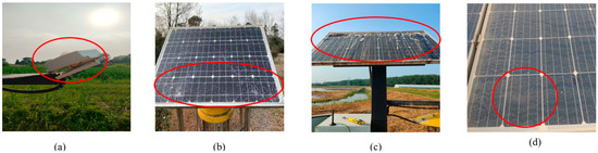
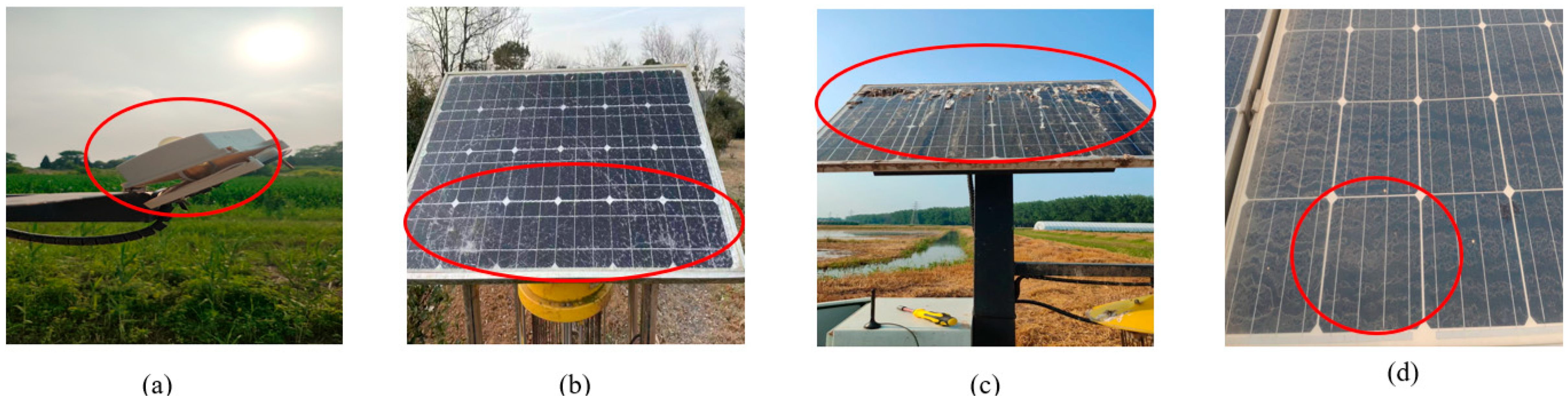
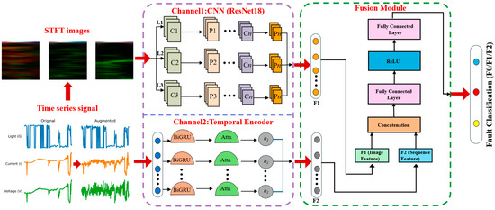
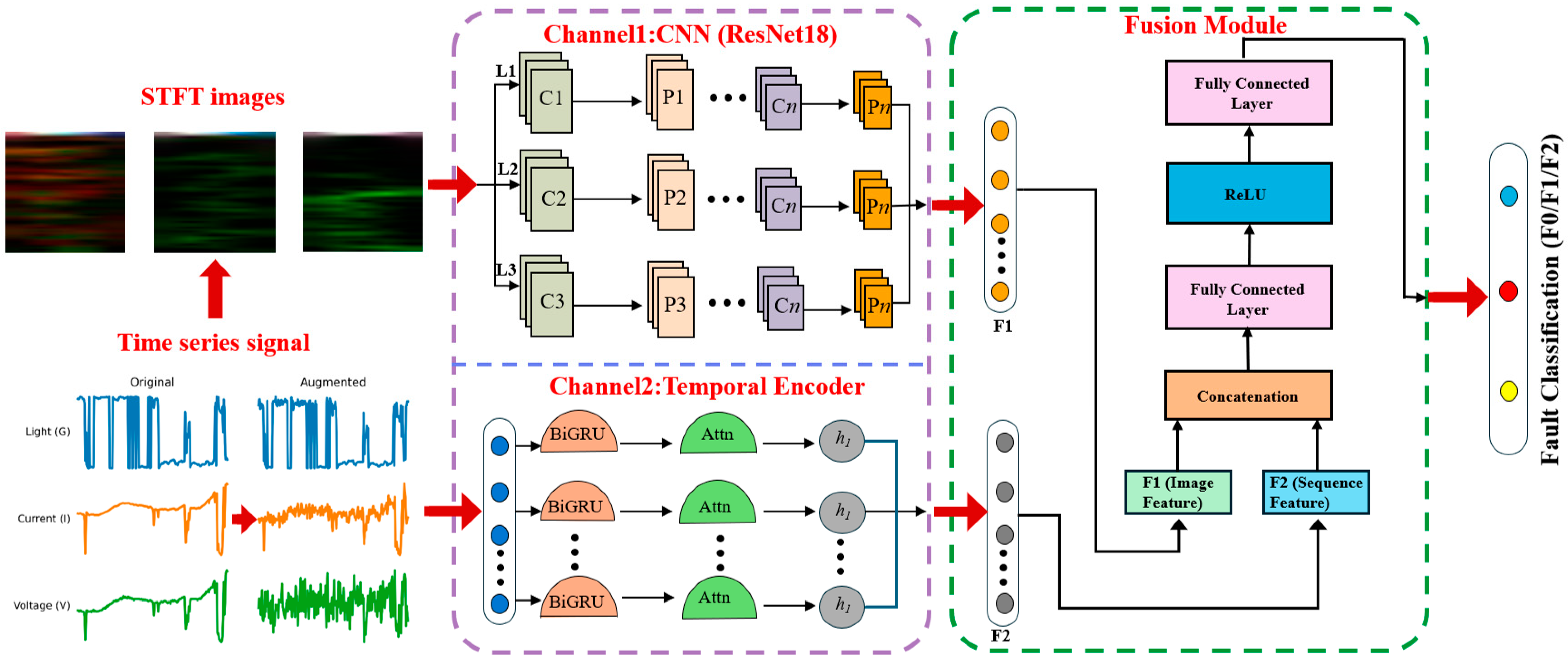
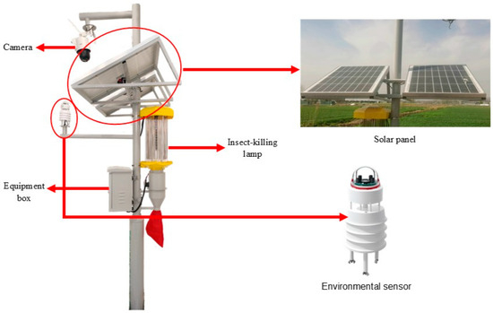
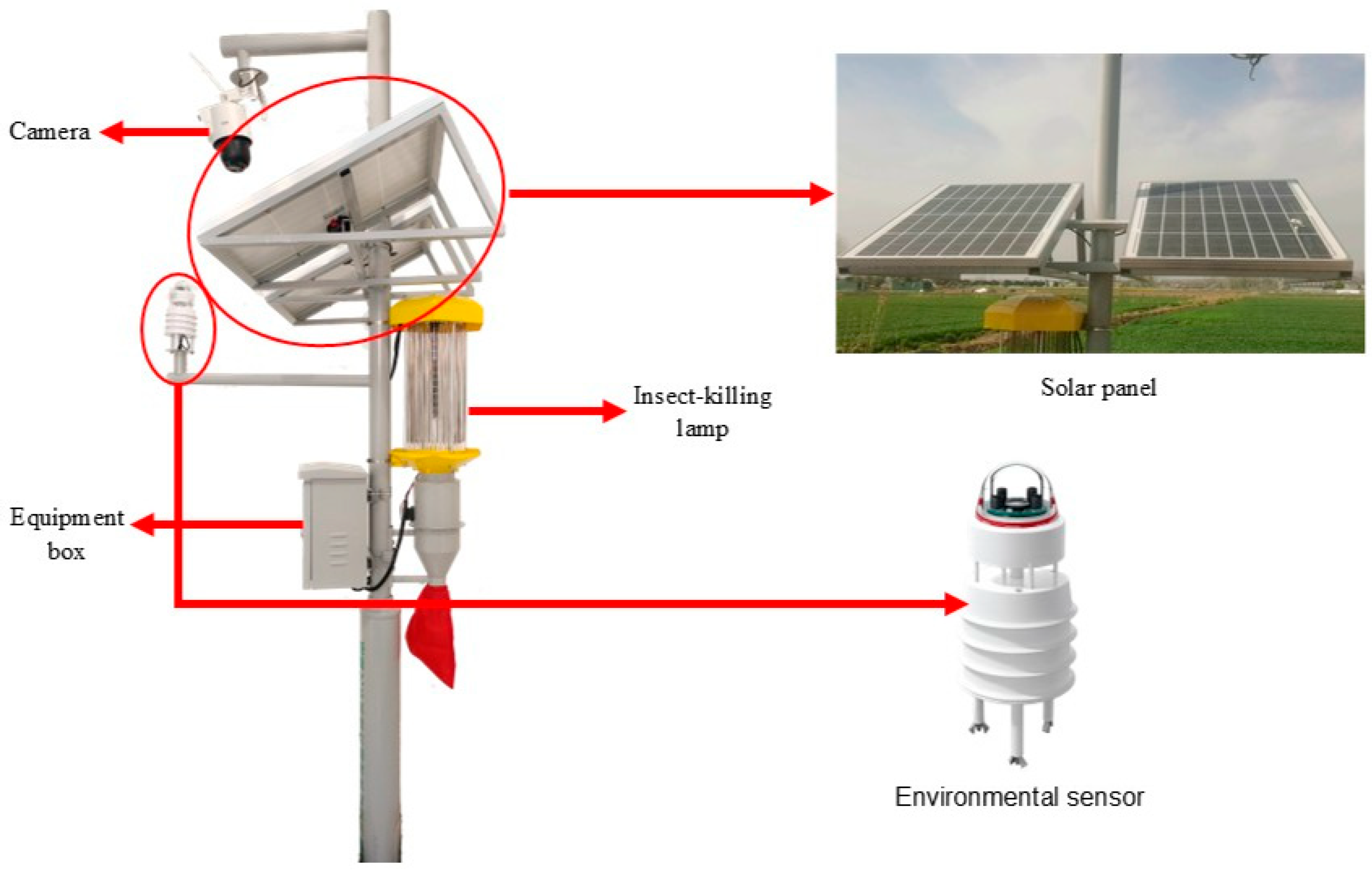
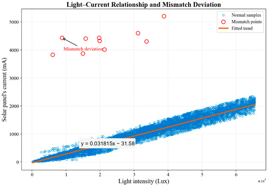
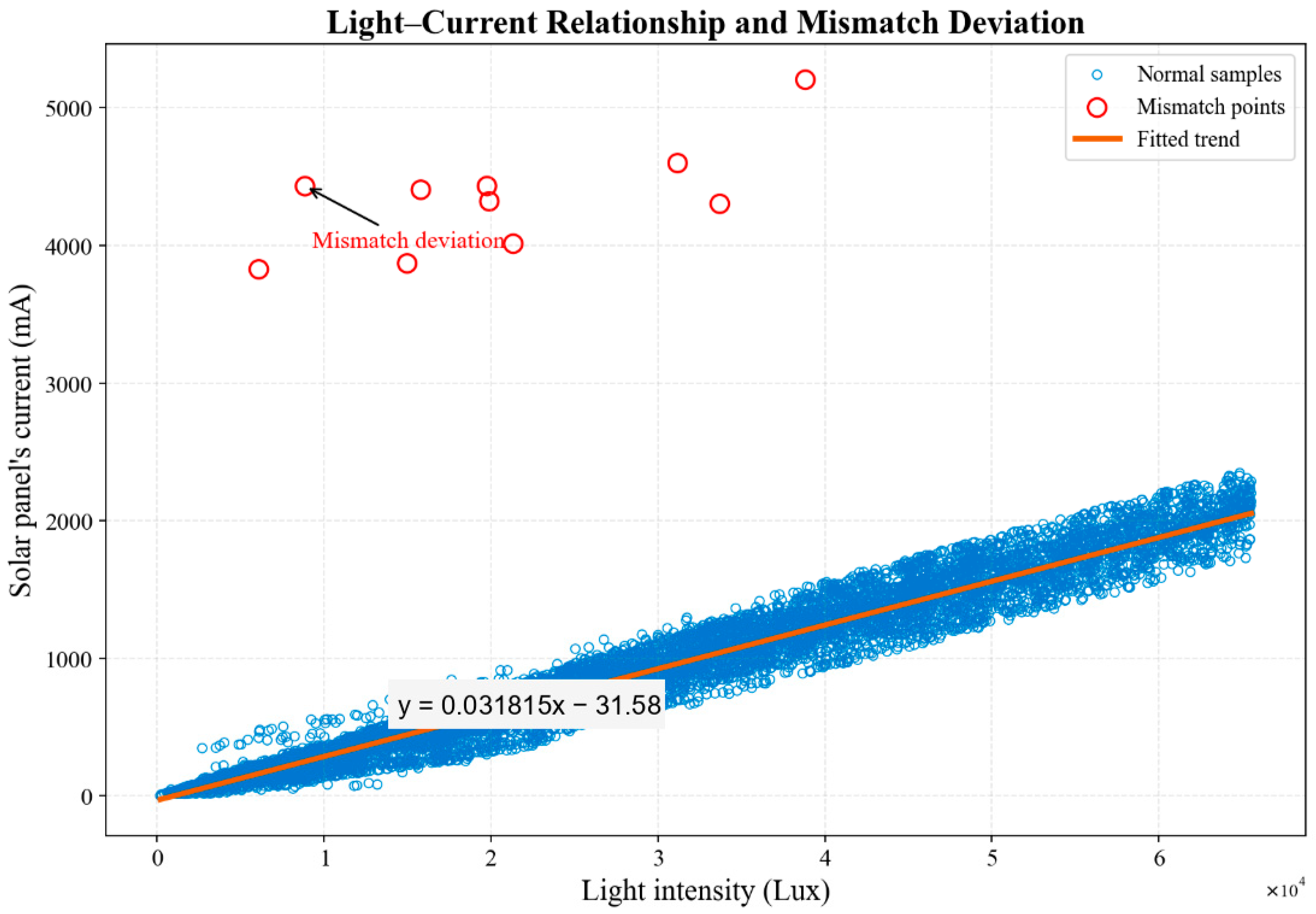
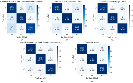
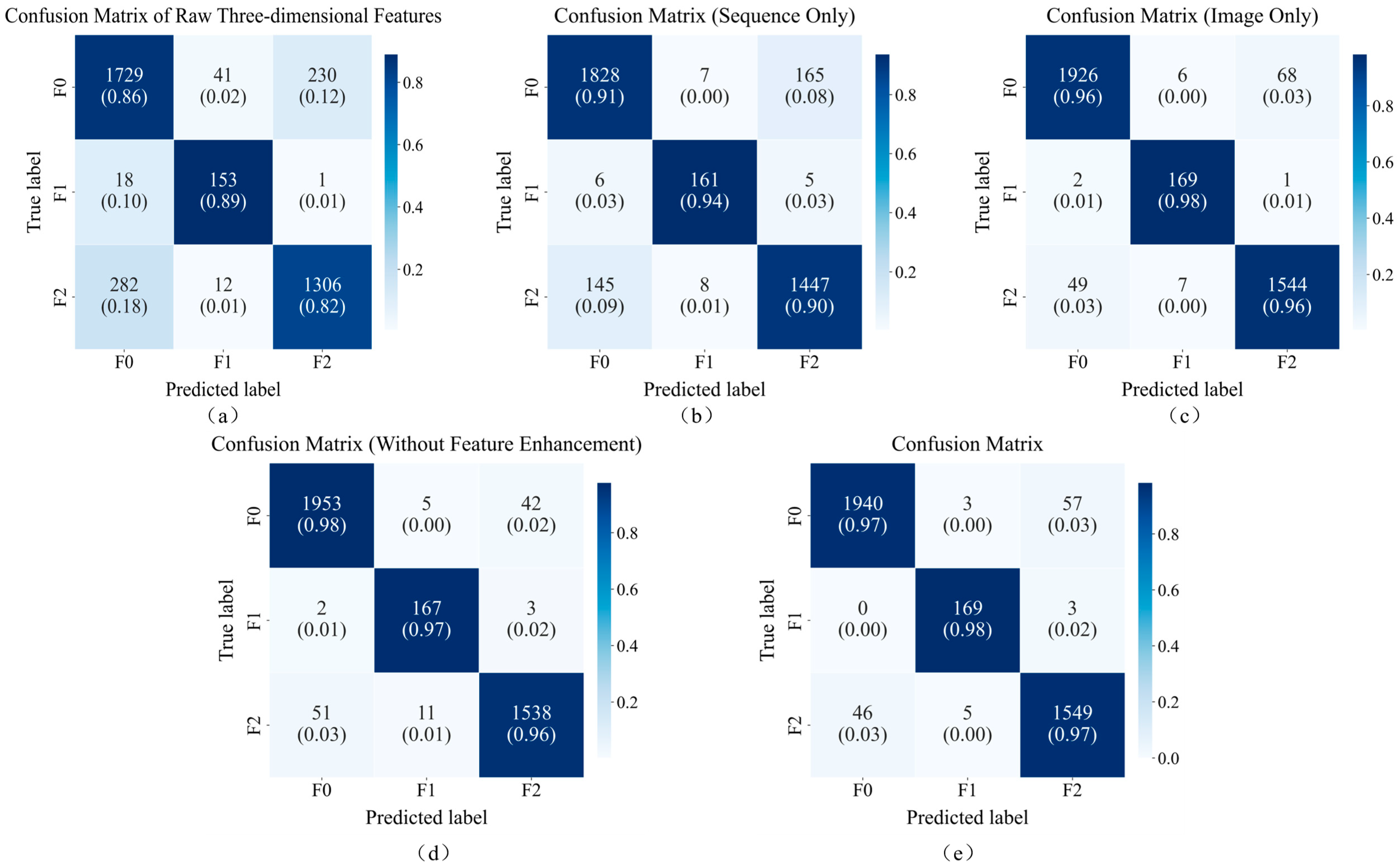
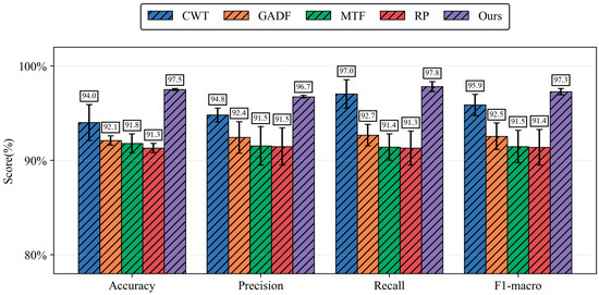
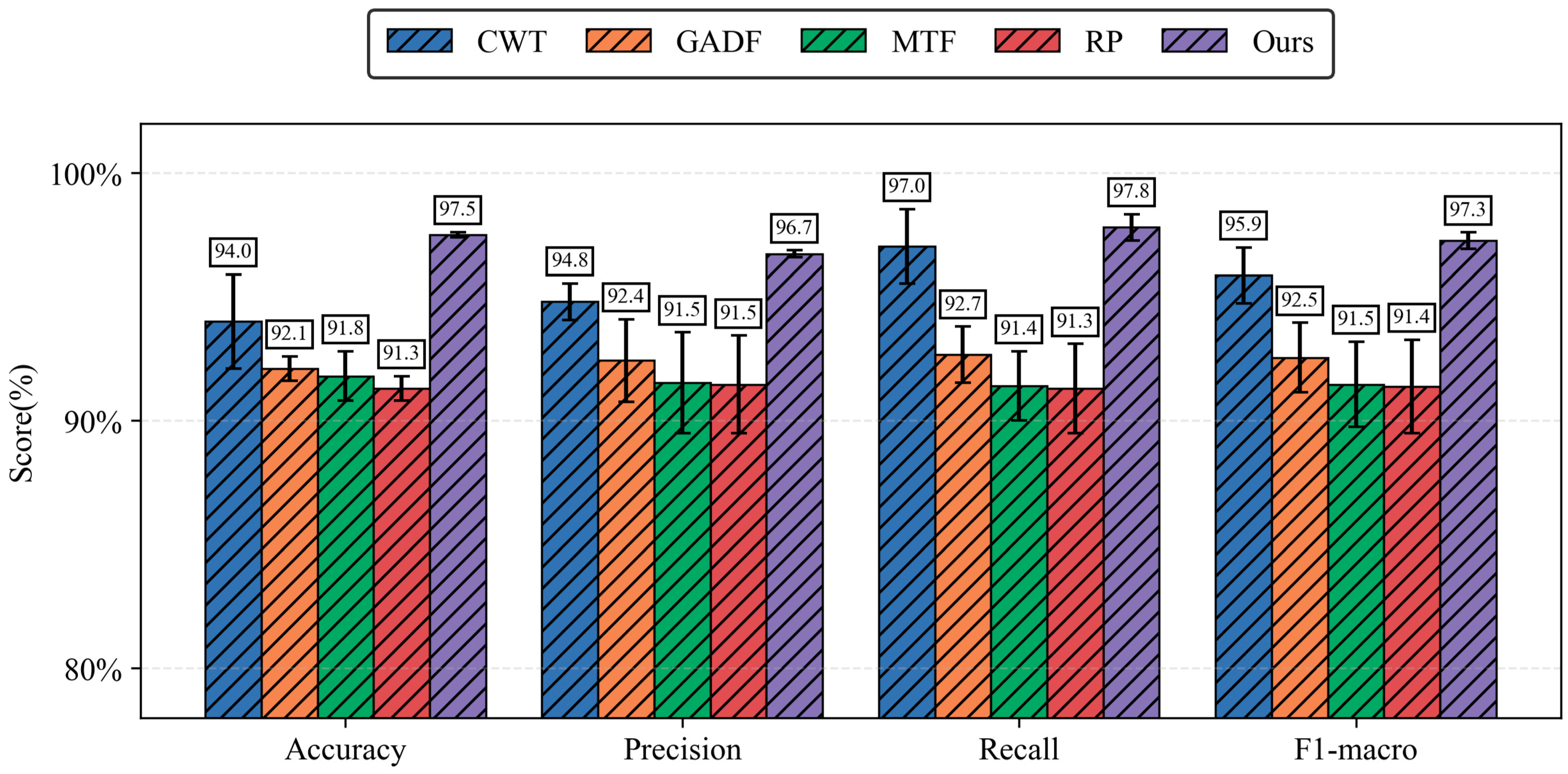
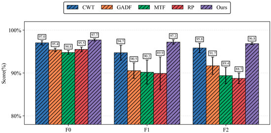
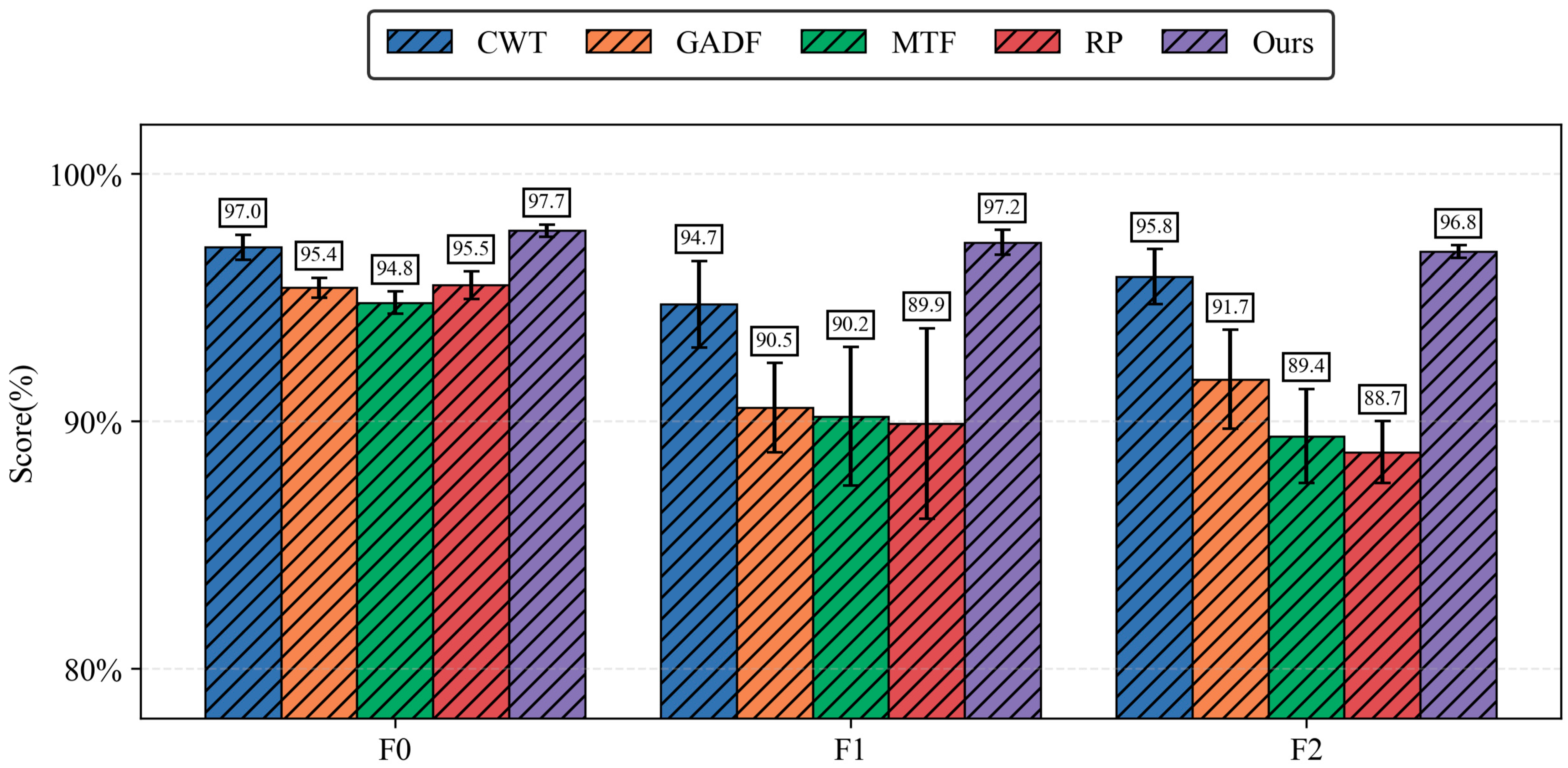
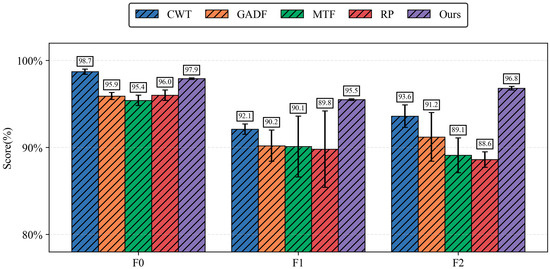
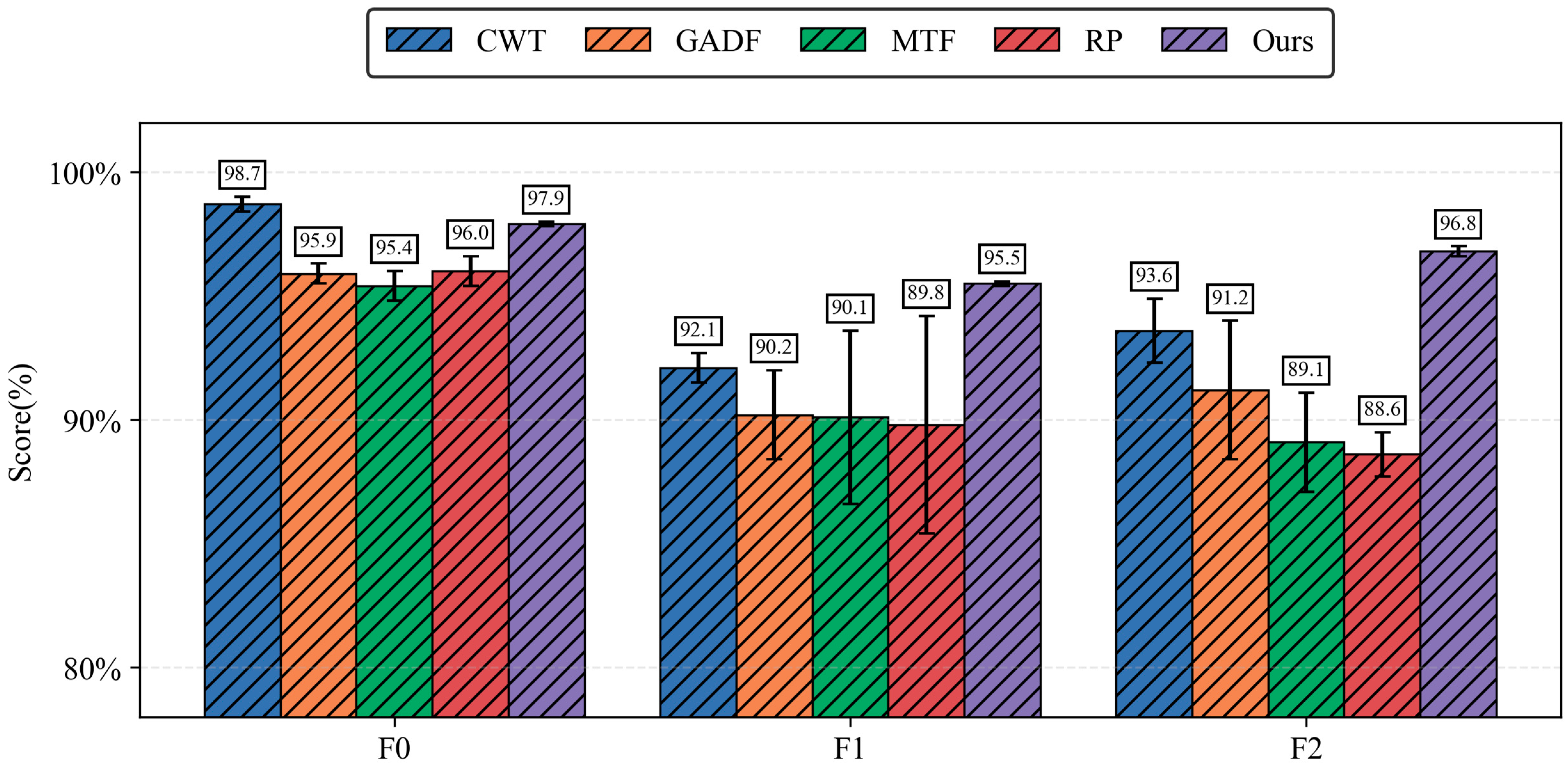
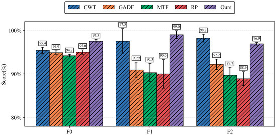
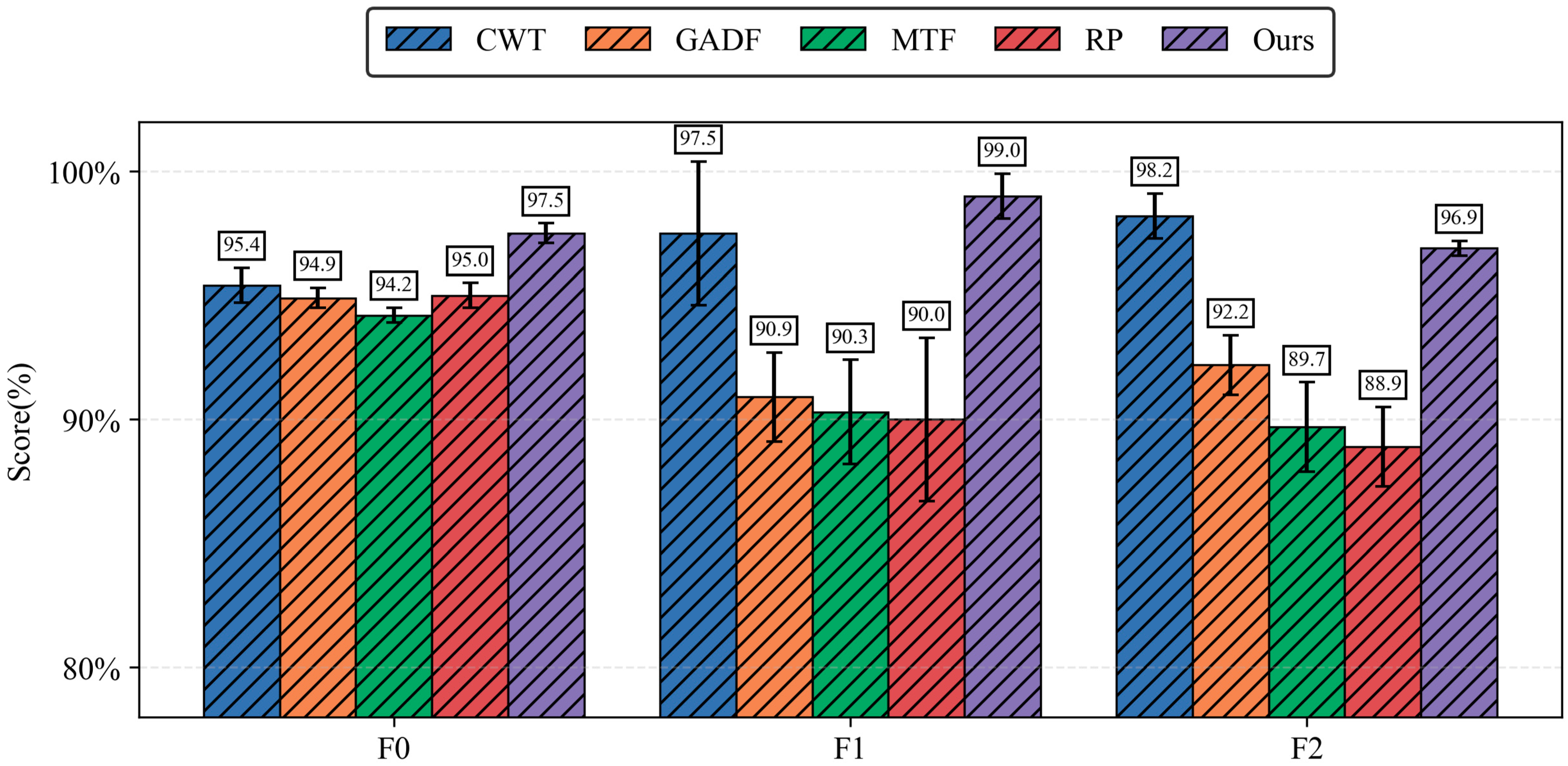
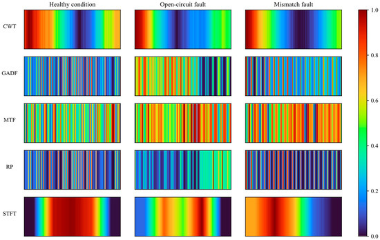
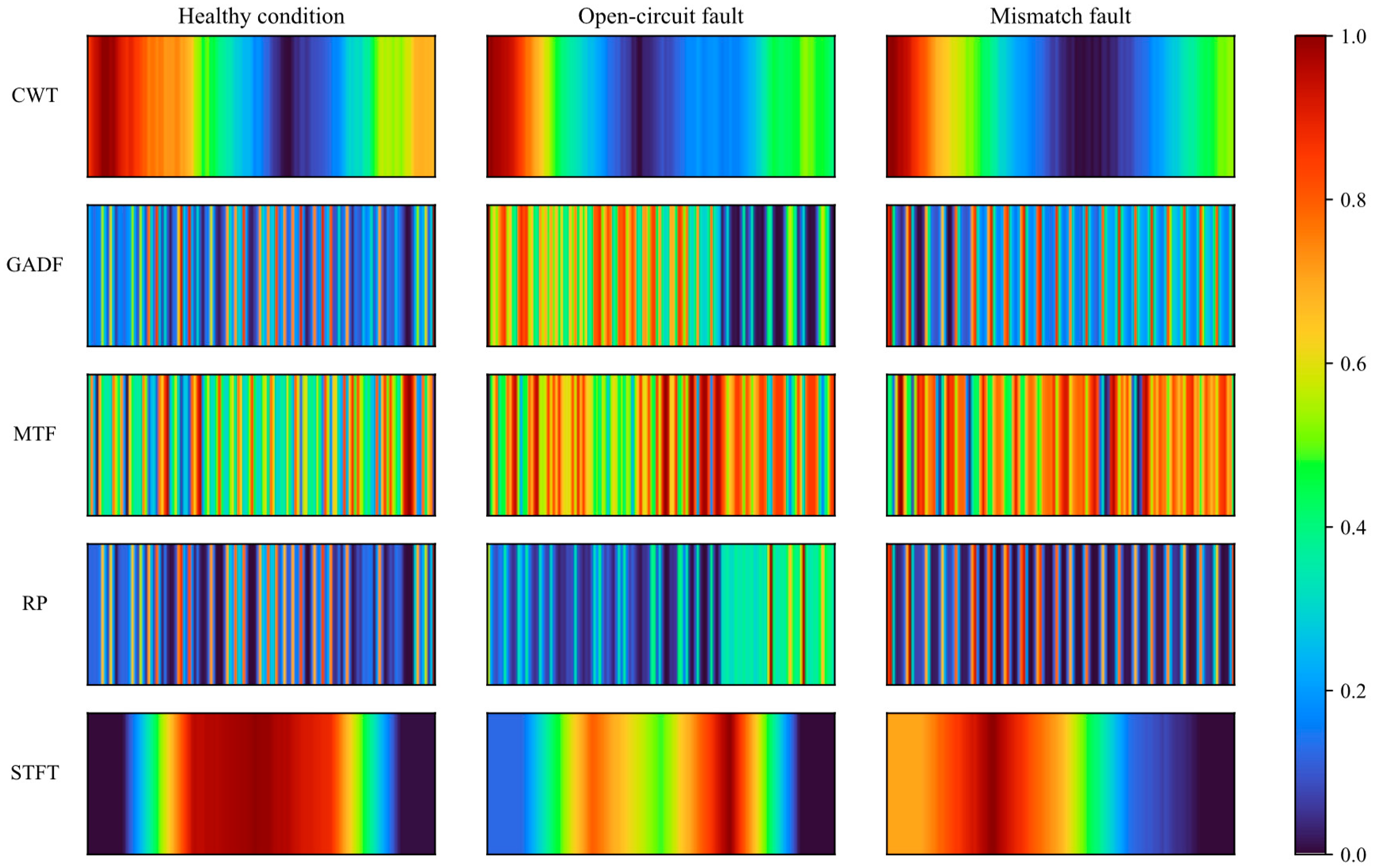
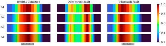
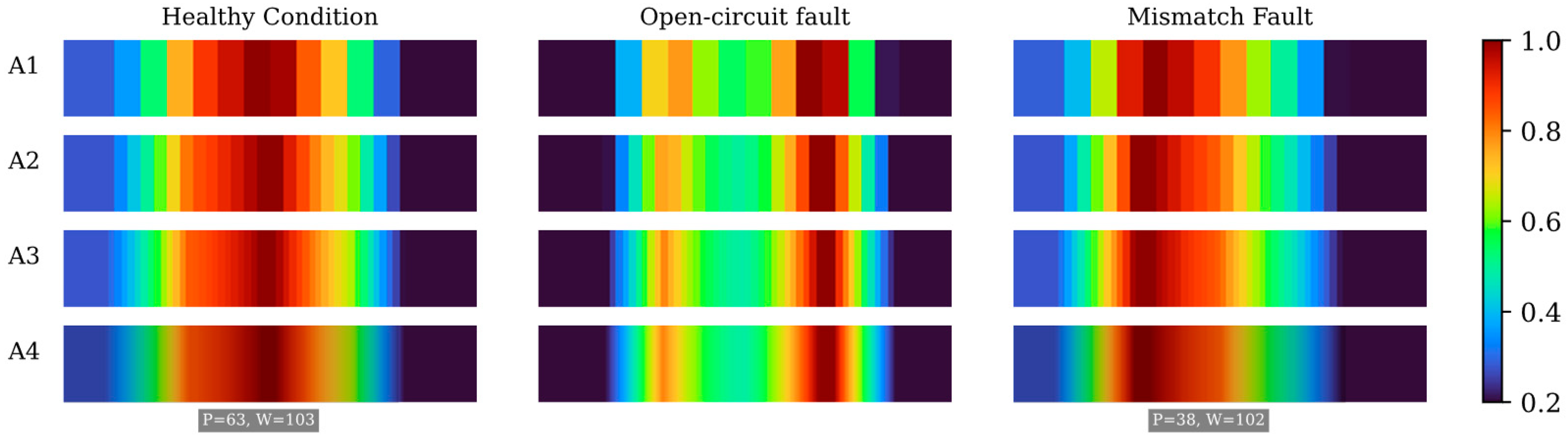
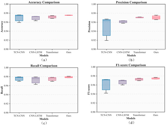
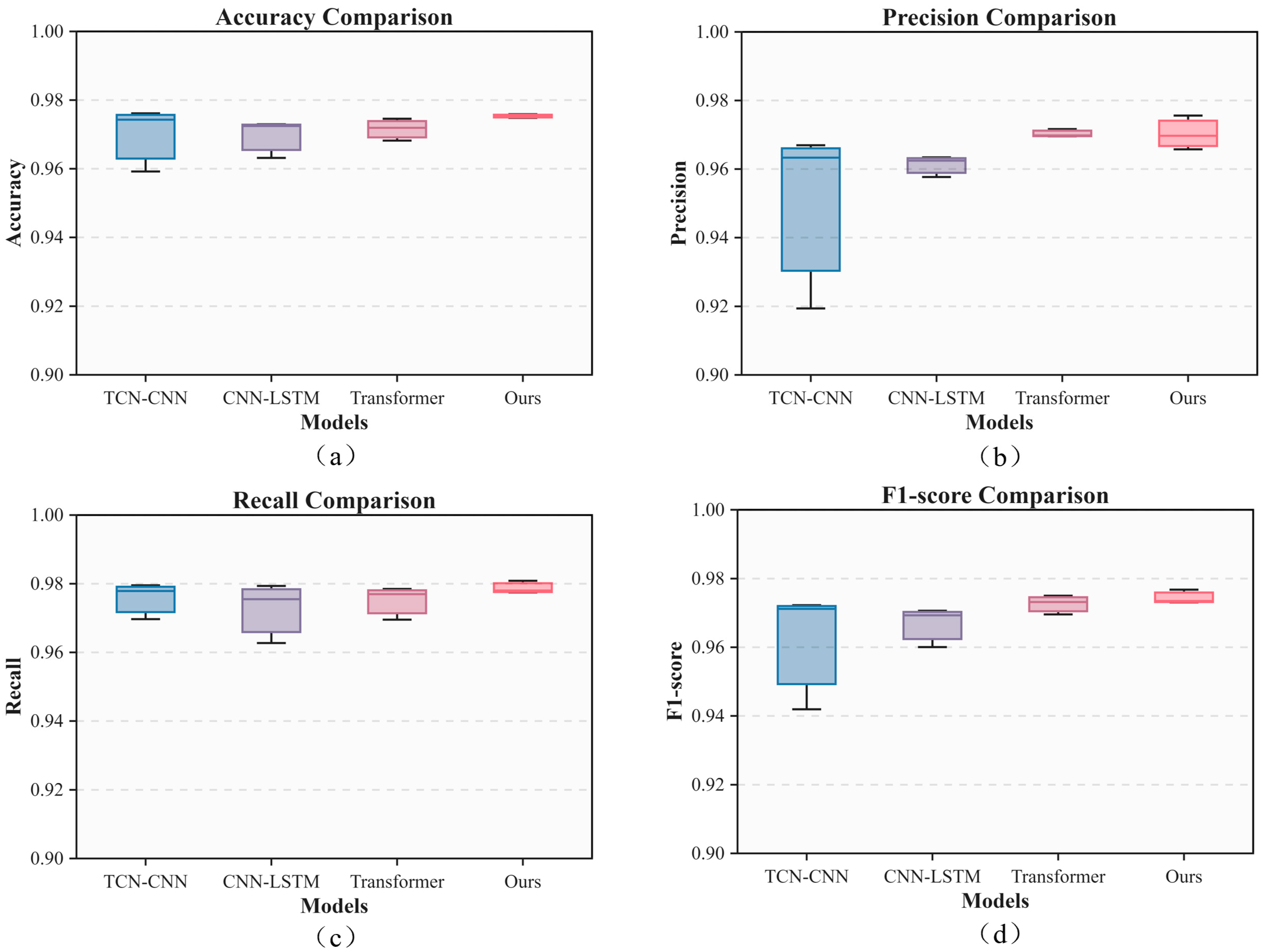
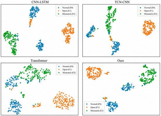
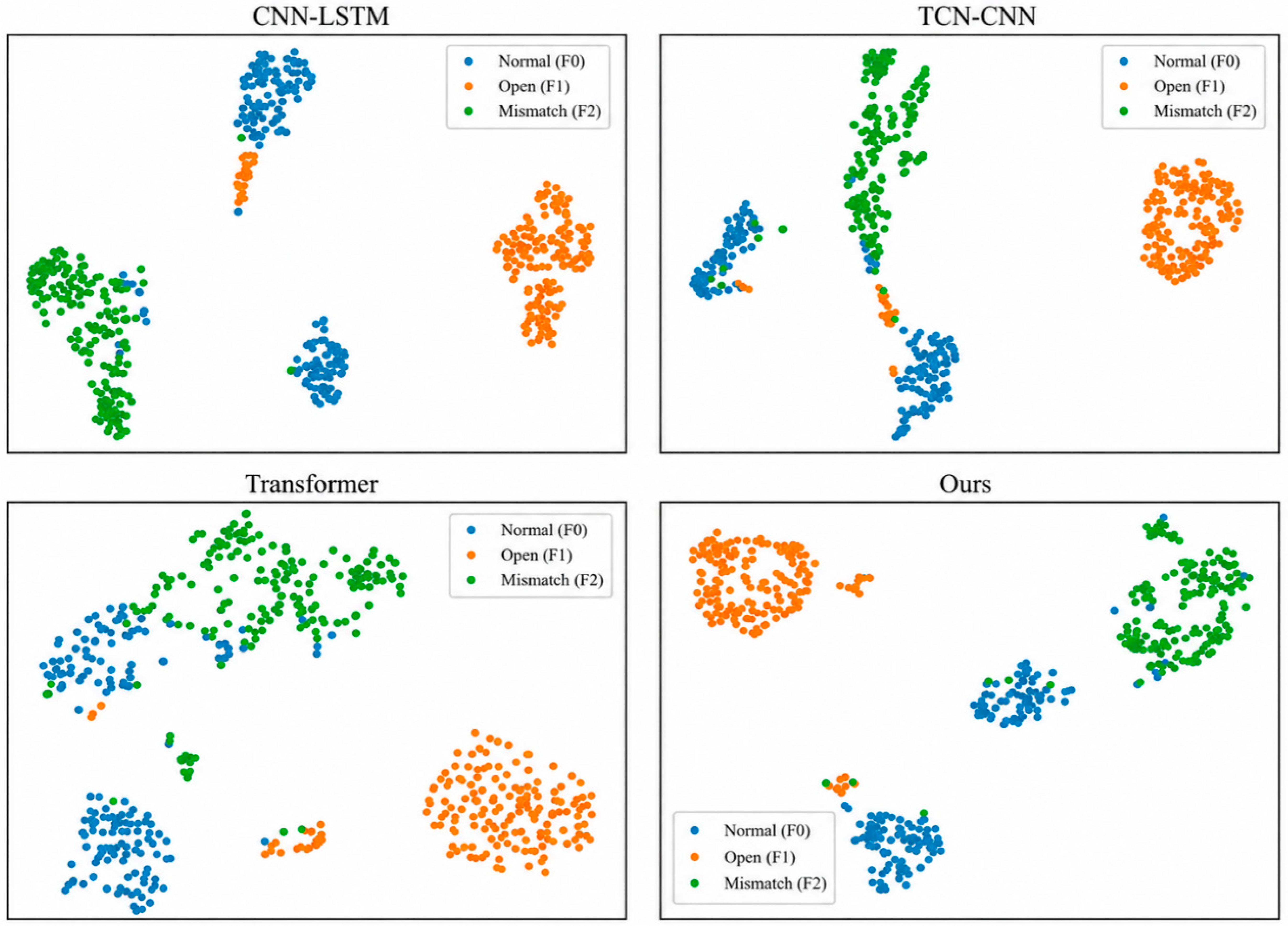

Disclaimer/Publisher’s Note: The statements, opinions and data contained in all publications are solely those of the individual author(s) and contributor(s) and not of MDPI and/or the editor(s). MDPI and/or the editor(s) disclaim responsibility for any injury to people or property resulting from any ideas, methods, instructions or products referred to in the content. |
© 2026 by the authors. Licensee MDPI, Basel, Switzerland. This article is an open access article distributed under the terms and conditions of the Creative Commons Attribution (CC BY) license.