Research on Intelligent Identification Method for Nitrogen Content in Greenhouse Cucumber Leaves Integrating YOLOv11n Segmentation and Machine Learning

Abstract

Rapid and non-destructive detection of nitrogen content in greenhouse cucumber leaves is essential for precision fertilization, yet traditional chemical methods are destructive and time-consuming, and existing spectral technologies suffer from high cost and poor field adaptability. This study aims to propose a high-precision detection scheme for cucumber leaf nitrogen content based on a lightweight model, suitable for complex scenarios. A total of 698 cucumber leaf images covering three growth stages were collected to build a segmentation dataset. Four categories and eight types of deep learning segmentation models were optimized and compared, and the optimal one was selected to extract leaf regions. Nine color features were extracted and combined with Kjeldahl-measured nitrogen content to construct and optimize three machine learning models, forming a deep learning segmentation–color feature extraction–machine learning prediction process. The results showed that YOLOv11n achieved the best segmentation accuracy, with an IoU of 0.9212 and AP of 0.9998 for high-resolution images. The optimized XGBoost had the highest prediction accuracy, with an MAE of 0.469, MSE of 0.461, and RMSE of 0.679, which are 10.15%, 8.71%, and 4.36% lower than Support Vector Regression with Radial Basis Function kernel (SVR_RBF) respectively, and its predicted nitrogen content aligned well with true values. The proposed scheme integrating YOLOv11n and XGBoost offers a lightweight technical solution for nitrogen nutrition diagnosis and precise fertilization of greenhouse cucumbers.

1. Introduction

Precision agriculture is the core direction of modern agricultural development [1]. Rapid and non-destructive acquisition of crop nutrient information is the key to realizing precision fertilization and improving crop yield and quality [2,3]. As a major vegetable crop under protected cultivation in China, cucumber, together with nitrogen (a macronutrient essential for crop growth) [4], directly affects photosynthetic efficiency, chlorophyll synthesis, and fruit development. Therefore, the accurate detection of leaf nitrogen content is crucial for the efficient cultivation of greenhouse cucumbers [5].

Traditional detection of crop nitrogen content relies on chemical methods such as the Kjeldahl method and dry ashing method. Although these methods offer high accuracy, they suffer from drawbacks including cumbersome operation, time-consuming and labor-intensive procedures, and destructive sampling, making it difficult to meet the requirements of real-time and large-scale field detection [6,7]. Therefore, exploring a lightweight, easy-to-operate, and field-adaptable method for rapid identification of nitrogen content in cucumber leaves is of great practical significance for the precision fertilization management of protected cucumber cultivation [8,9].

Sabzi et al. [10] proposed a hyperspectral imaging framework integrating a hybrid artificial neural network and imperialist competitive algorithm (ANN-ICA) to detect 30% excess nitrogen in cucumber plants. The wavelengths of 715 nm, 783 nm, and 821 nm were identified as the optimal diagnostic bands via the hybrid artificial neural network and artificial bee colony algorithm (ANN-ABC). The model achieved a classification accuracy of 96.11%, and statistically significant spectral differences were detectable as early as one day after the application of excess nitrogen. Hou et al. [11] employed cosine similarity analysis and identified that the edge, vicinity of the main vein, and leaf base regions of cucumber leaves are unstable spectral areas when Raman Spectroscopy (RS) is used for diagnosing early nitrogen (N), phosphorus (P), and potassium (K) deficiency. After excluding these low-similarity data, the F1 score of the Partial Least Squares-Discriminant Analysis (PLS-DA) model under 24-h early stress increased from 91.20% to 93.30%, and the number of misdiagnoses decreased from 15 to 8. In their subsequent research, the team constructed a quantitative Raman spectroscopy model for nitrogen content. Among the proposed strategies, the optimal scheme combining iterative polynomial fitting, four-dimensional feature extraction, and competitive adaptive reweighted sampling (CARS) achieved a coefficient of determination (R²) of 0.847 for the prediction set and a residual predictive deviation (RPD) of 2.555 [12]. These studies verify that hyperspectral and Raman spectroscopy coupled with targeted chemometric algorithms enable high-accuracy, non-destructive cucumber nitrogen status detection for precision agriculture.

Although the aforementioned non-destructive detection technologies such as hyperspectral imaging and chlorophyll fluorescence have improved detection efficiency, they are difficult to popularize on a large scale in planting fields due to their high equipment costs and poor environmental adaptability [13].

Leaf color is an intuitive external characterization of crop nitrogen nutritional status. Extracting leaf color features and combining them with machine learning algorithms is a low-cost and effective approach to obtaining the nitrogen content in cucumber leaves [14,15,16]. However, field cucumber leaf images are easily affected by complex background interference such as branches, weeds, and soil, as well as problems including leaf overlap, occlusion, and uneven illumination, which seriously affect the accuracy of crop leaf segmentation and color feature extraction [17,18,19]. With the rapid development of deep learning technology, image segmentation models such as Mask R-CNN, DeepLab v3+, and FCN [20,21,22,23] have exhibited strong feature extraction and pixel-level segmentation capabilities. These models can effectively separate complex backgrounds and accurately locate leaf regions, providing an effective solution for cucumber region segmentation in complex scenarios.

In recent years, scholars at home and abroad have conducted extensive research on the non-destructive identification of crop nitrogen content. To address the problems of dense overlap of cucumber leaves and complex illumination in top-view images of greenhouse canopies, Qian et al. proposed a segmentation method based on a dual-layer convolutional network (BCNet). They introduced the Convolutional Block Attention Module (CBAM) to enhance the ability of edge feature extraction and replaced Focal Loss with Varifocal Loss to optimize the performance of dense object detection. Finally, in glass greenhouse and plastic greenhouse scenarios, the average precision (AP) of leaf object detection reached 96.57% and 96.86%, respectively, and the AP of instance segmentation reached 84.71% and 83.27%, respectively, outperforming mainstream models such as Faster R-CNN, Mask R-CNN, and YOLOv4 [24].

To achieve universal detection of gray mold in three crops (tomato, pepper, and cucumber), Medentzidis et al. [25] adopted a two-stage architecture. In the first stage, YOLOv11L-seg was used for single-class leaf instance segmentation, achieving a mean Average Precision at 50 intersection over union (mAP@50) of 87.3% and a mean Dice Similarity Coefficient (mDSC) of 86.0%. In the second stage, a soft voting ensemble of 13 MobileViT variant models was employed for classification, resulting in an overall F1-score of 84.05%, with an F1-score of 70.55% for diseased cucumber leaves. This method enables multi-crop leaf segmentation and disease detection using only RGB data, demonstrating potential for deployment on smartphone devices.

To address the demand for grading the severity of cucumber diseases under natural environments, Yao et al. [26] proposed a two-stage segmentation framework (TUNet) integrating TRNet and U-Net. In the first stage, TRNet, which combines ResNet50 and Transformer, was used to segment target leaves, achieving an accuracy of 93.94% and a Dice coefficient of 96.98%, effectively solving the problems of leaf overlap and complex background interference. In the second stage, U-Net with ResNet50 as the backbone was adopted to segment disease lesions, with a Dice coefficient of 68.14%. Finally, the average accuracy for grading the severity of cucumber downy mildew and anthracnose reached 94.49% and 94.43%, respectively, which were 4.71% and 8.08% higher than those of DUNet and BLSNet. This provides a quantitative basis for precise pesticide spraying.

Facing the complex illumination environment of fully artificial light plant factories, Zhang et al. [27] improved YOLOv8 to obtain the CL-YOLOv8 model. They replaced the bottleneck structure of the original C2f module with a Multi-Scale Feature Module (MSFM) and introduced the Efficient Multi-scale Attention (EMA) mechanism to enhance illumination robustness. Meanwhile, an Efficient Sub-Pixel Upsampling Block (ESPUB) was designed to improve the resolution of feature maps while reducing computational overhead. Ultimately, the model achieved a mean Average Precision at 50 intersection over union (mAP@50) of 0.914 for segmentation tasks, which was 2.4% higher than that of the baseline YOLOv8-seg, and an mAP@50:95 of 0.829, outperforming comparative models such as YOLOv5-seg, YOLOv7-seg, and Mask R-CNN. It is suitable for real-time monitoring requirements of embedded devices in plant factories. Currently, there is a lack of integrated lightweight and high-precision detection schemes suitable for complex backgrounds in cucumber nitrogen assessment. Thus, exploring relevant technologies is crucial for advancing precision fertilization practices in greenhouse environments.

Considering the lightweight characteristics of YOLOv11, its fusion with machine learning models offers a feasible solution tailored for resource-constrained scenarios. Taking greenhouse cucumbers in Xinjiang as the research object, this study collected leaf images in multiple scenarios (seedling stage, flowering stage, and fruiting stage) to construct a cucumber leaf segmentation dataset under complex backgrounds. Four categories and eight deep learning segmentation models were optimized and compared, and the optimal model was selected to achieve accurate extraction of leaf regions. Based on the segmentation results, nine color features were extracted. Combined with the nitrogen content measured by the Kjeldahl method, three machine learning recognition models were constructed and their hyperparameters were optimized. A complete lightweight detection process for cucumber leaf nitrogen content, implemented via the ‘deep learning segmentation—color feature extraction—machine learning prediction’ pipeline, was established.

The main contributions of this paper are as follows:

• This study evaluated eight mainstream segmentation models for cucumber leaf segmentation under complex backgrounds, demonstrating that standard YOLOv11n achieves optimal accuracy and efficiency, outperforming DeepLab v3+, FCN and Mask R-CNN, and surpassing existing optimized YOLO models for embedded plant factory monitoring.
• We proposed a lightweight pipeline utilizing compact YOLOv11n and XGBoost for cucumber nitrogen prediction. Replacing expensive spectral systems with standard imaging, the framework achieves optimal performance, offering a viable solution for cost-effective greenhouse management.

2. Materials and Methods

2.1. Dataset Construction and Annotation

Cucumber is a dominant protected cultivation crop in China. From March to June 2023, a total of 698 cucumber leaf images with a resolution of 4080 × 3060 pixels were collected at the experimental base of the Xinjiang Academy of Agricultural Sciences, covering the seedling, flowering, and fruiting stages under varying weather conditions, at different time points, and across multiple greenhouse locations.

The Labelme 5.2.1 software was used to annotate precise leaf regions against complex backgrounds for segmentation tasks. After manual annotation, corresponding JSON files were generated and converted into COCO-formatted datasets suitable for deep learning models. After manual annotation of the cucumber leaves was completed and the corresponding JSON files were generated, both the detection and segmentation datasets were randomly partitioned into training, validation, and test sets. The JSON file was then converted into a COCO-formatted dataset suitable for deep learning models. The cucumber leaf image dataset was randomly divided into training, validation, and test sets at a ratio of 500:100:98.

The cucumber leaf detection model was trained on a Windows 10 operating system, equipped with an Intel Core i5-8500 @ 3.00 GHz 6-core CPU (Santa Clara, CA, USA), an NVIDIA GeForce RTX 3060 Laptop GPU, and 16 GB of ROM (NVIDIA Corporation, Santa Clara, CA, USA). The integrated development environment comprised PyCharm Community Edition 2021, CUDA 11.0, and cuDNN 8.0, with the PyTorch 1.7.1 deep learning framework and Python 3.8.17 as the programming language. The YOLOv11 segmentation model was trained and tested on a cloud server equipped with an NVIDIA GeForce RTX 5090 with 32,109 MiB of memory (NVIDIA Corporation, Santa Clara, CA, USA), running torch-2.8.0, CUDA 12.8, Python 3.12.3, and Ultralytics 8.3.0.

2.2. Cucumber Leaf Segmentation Models

2.2.1. Mask R-CNN Architecture and Model Implementation for Cucumber Leaf Segmentation

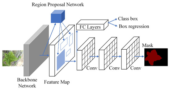
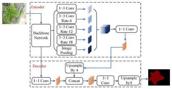
The Mask R-CNN algorithm integrates the object detection framework Faster R-CNN with the Fully Convolutional Network (FCN) for feature extraction and classification [28], as illustrated in Figure 1. First, Faster R-CNN generates candidate regions through a Region Proposal Network (RPN), and the FCN extracts features from candidate regions and performs classification. The training process adopts a loss function analogous to that of Faster R-CNN, establishing the algorithm as a widely adopted segmentation framework [29].

Figure 1. Mask R-CNN working architecture.

For the cucumber leaf segmentation task, a dedicated model was constructed based on pre-trained weights from the COCO dataset. To enhance training efficiency, all input cucumber leaf images were resized to 400 × 300 pixels. The training procedure was divided into two sequential stages: First, the backbone network was frozen, and only the network head was trained for 50 epochs with a batch size of 8. Second, the entire network was trained for 300 epochs with a batch size of 8, and the number of target classes (num_class) was set to 2, including background and cucumber leaf.

2.2.2. DeepLab v3+ Architecture and Implementation for Cucumber Leaf Segmentation

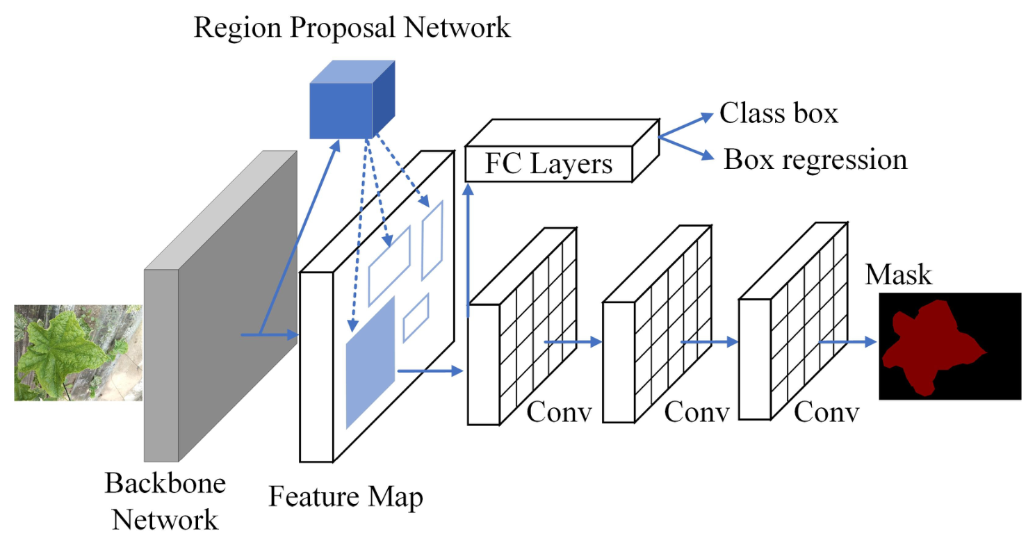
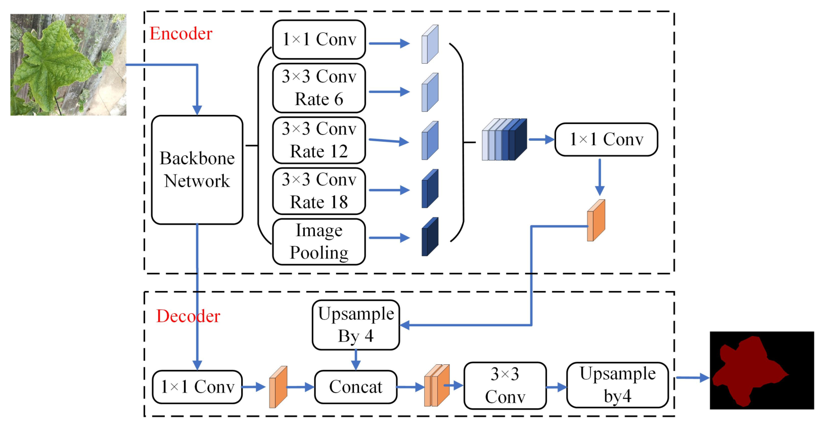
The DeepLab semantic segmentation algorithm employs a spatial pooling module and an encoder–decoder architecture. The pyramid module enriches contextual information through pooling operations, while the encoder–decoder architecture restores the boundary details of segmented regions [30]. Compared to Fully Convolutional Networks, this algorithm expands the receptive field by increasing the sparsity of convolution kernels while preserving internal data structures and preventing feature loss during downsampling. Leveraging the spatial pyramid pooling structure, Atrous convolution with varying dilation rates is utilized to fuse multi-scale information, resulting in the high-performance DeepLab v3+ network architecture [31], as illustrated in Figure 2.

Figure 2. DeepLab v3+ working architecture.

For the DeepLab v3+ image segmentation network, two lightweight deep convolutional neural networks, MobileNetv2 and Xception, were adopted as backbone networks. Two DeepLab v3+ models were constructed based on pre-trained weights from the VOC dataset. To enhance training efficiency, all input cucumber leaf images were resized to 400 × 300 pixels. The training strategy was divided into two sequential steps. First, the backbone feature extraction network was frozen with a batch size of 8, an initial learning rate of 0.00001, and freeze_epochs set to 50. Second, the entire network was unfrozen for training, with Unfrozen_epochs set to 200 and the batch size set to 8.

2.2.3. FCN Architecture and Implementation for Cucumber Leaf Segmentation

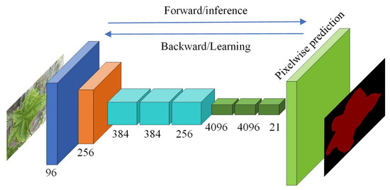
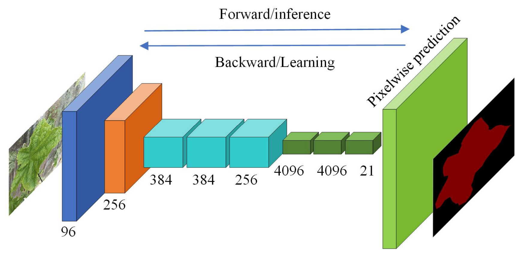
The FCN is an early semantic segmentation model characterized by replacing the fully connected layers of a standard CNN with convolutional layers, thereby eliminating spatial dimensionality reduction. It utilizes upsampling for dense prediction and combines deconvolution with fully connected layers to achieve per-pixel classification [32]. Common deep convolutional network architectures used as the backbone for FCNs—such as LeNet, AlexNet, VGG-16, VGG-19, and GoogleNet—typically consist of an input layer, convolutional layers, pooling layers, ReLU layers, fully connected layers, and an output layer. By sharing weights between convolution kernels and filters, these networks achieve excellent performance in object detection, image classification, and natural language processing. The network structure of the FCN algorithm is illustrated in Figure 3.

Figure 3. FCN working architecture.

For the FCN semantic segmentation algorithm, a cucumber leaf segmentation model was constructed using the classic deep convolutional network VGG-19 as the backbone, initialized with pre-trained weights from the MS COCO dataset. To improve training efficiency, all input cucumber leaf images were resized to 400 × 300 pixels. The Adam optimizer was selected for model training, with a learning rate of 0.0001, num_classes set to 2, batch_size set to 2, and epochs set to 300.

2.2.4. YOLOv11 Architecture and Implementation for Cucumber Leaf Segmentation

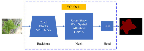
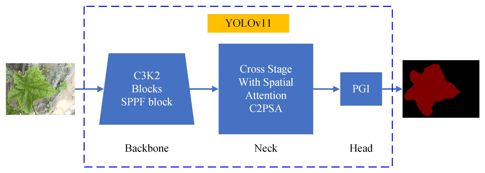
YOLOv11 achieves significant structural upgrades by replacing the previous C2f block with the efficient C3k2 Cross Stage Partial (CSP) module, as illustrated in Figure 4. Equipped with two small convolutions rather than a single large convolution, the C3k2 block adopts a smaller kernel size to accelerate inference speed while maintaining competitive model performance. Additionally, two novel blocks are introduced to enhance feature extraction capability: the C2PSA block strengthens spatial attention on critical image regions, and the SPFF block optimizes multi-scale feature fusion to improve detection accuracy for objects with diverse sizes and positions [33].

Figure 4. YOLOv11 working architecture.

The YOLOv11 series comprises five model variants (nano, small, medium, large, and extra-large) tailored for different application scenarios. In this study, the first four variants were selected for model training. To balance model convergence efficiency and generalization capability, the training hyperparameters were configured as follows: the total number of training epochs was set to 200, the input image size was uniformly resized to 640 × 640 pixels, the batch size was set to 32, and the number of data loading workers was set to 8 to accelerate data preprocessing.

To prevent overfitting, an early stopping mechanism was adopted, which terminates the training process when the validation set loss fails to decrease for 30 consecutive epochs. Meanwhile, model weights were saved every 10 epochs to facilitate subsequent model selection and comparative analysis. To enhance model robustness, data augmentation strategies were enabled, and the MixUp augmentation technique was introduced with a mixing ratio of 0.1. Furthermore, the model was initialized with pre-trained weights to accelerate convergence and improve final detection accuracy via transfer learning.

2.2.5. Evaluation Metrics for Cucumber Leaf Segmentation

The performance of the cucumber leaf image segmentation model is evaluated using four core metrics: Intersection over Union (IoU), Precision (P), Recall (R), and Pixel Accuracy (A), adopted as the primary benchmark following the standard practice in agricultural image segmentation studies [34].

The IoU quantifies the overlap between the predicted segmentation mask (or bounding box) and the ground truth annotation, calculated as the ratio of the intersection area to the union area of the two regions:

$$IOU=TP/(TP+FN+FP)$$

(1)

where True Positive (TP) indicates correctly predicted positive pixels, False Positive (FP) indicates pixels incorrectly predicted as positive, and False Negative (FN) indicates positive pixels missed by the prediction.

Precision (P) measures the proportion of pixels predicted as cucumber leaf (or lesion) that are correctly labeled, calculated as

$$P=TP/(TP+FP)$$

(2)

Recall (R) measures the proportion of actual positive pixels that are successfully identified by the model, calculated as

$$R=TP/(TP+FN)$$

(3)

Pixel Accuracy (A) refers to the ratio of correctly classified pixels to the total number of pixels in the image, including both foreground (leaf/lesion) and background categories, formulated as:

$$A=(TP+TN)/(TP+FP+FN+TN)$$

(4)

where p_ii indicates the number of pixels correctly classified into class i, and p_ij indicates the number of pixels belonging to class i but predicted as class j.

2.3. Intelligent Model for Identifying Nitrogen Fertiliser Content in Cucumber Leaves Based on Colour Characteristics

2.3.1. Leaf Sample Collection and Nitrogen Content Determination

Leaf samples for the cucumber leaf nitrogen content identification model were collected during the flowering, fruiting, and ripening stages. During each growth stage, fifty cucumber leaves were randomly collected from different plants at various locations within the greenhouse, yielding a total of 150 leaf samples. The collected leaves were placed in resealable bags and transported to the laboratory. They were subjected to a blanching treatment in a vacuum drying oven at 105 °C to inactivate enzymes, after which the dried leaves were pulverized for nitrogen content analysis.

This study employed a Kjeldahl nitrogen analyzer (KDN-520, Hangzhou Greenbo Instruments Co., Ltd., Hangzhou, China). The determination procedure comprised three stages: digestion, distillation, and titration. During the digestion stage, concentrated sulfuric acid and copper sulfate were mixed with the crushed cucumber leaf powder under high-temperature, strong-acid conditions, which produced ammonium sulfate. During distillation, the digested ammonium sulfate reacted under high-temperature and alkaline conditions to produce ammonia gas and water vapor, which was then collected using a boric acid solution. Finally, the boric acid solution containing the ammonia gas, along with a bromocresol green-methyl red indicator, was titrated with a hydrochloric acid solution. The nitrogen content in the sample leaves was determined based on the volume of hydrochloric acid titrated [35]. The chemical equations for the three processes are as follows:

Digestion process:

$${2NH}_4^{+}+H_2{SO}_4+2H^{+}={\left({NH}_4\right)}_2{SO}_4$$

(5)

Distillation process:

$${\left({NH}_4\right)}_2{SO}_4+2NaOH=2{NH}_3\uparrow +2H_{2}O+{Na}_2{SO}_4$$

(6)

$${4H_{3}BO}_3+2{NH}_3=5H_{2}O+{\left({NH}_4\right)}_2{B}_4{O}_7$$

(7)

Titration process:

$${\left({NH}_4\right)}_2{B}_4{O}_7+H_2{SO}_4+5H_{2}O={\left({NH}_4\right)}_2{SO}_4+{4H_{3}BO}_3$$

(8)

$${\left({NH}_4\right)}_2{B}_4{O}_7+2HCl+5H_{2}O=2{NH}_{4}Cl+{4H_{3}BO}_3$$

(9)

where ${\mathrm{N}\mathrm{H}}_4^{+}$ indicates ammonium ion, H₂SO₄ indicates concentrated sulfuric acid; H⁺ indicates hydrochloric acid ion, (NH₄)₂SO₄ indicates ammonium sulfate, NaOH indicates Sodium hydroxide, NH₃ indicates ammonia, H₂O indicates water vapor, Na₂SO₄ indicates sodium sulfate, H₃BO₃ indicates Boric acid, (NH₄)₂B₄O₇ indicates Ammonium borate, HCl indicates Hydrochloric acid.

Initially, the digestion furnace temperature is set to 280 °C. After digestion for 30 min, the temperature was increased to 350 °C. Following a subsequent 60 min digestion period, the temperature was raised to 450 °C for a final 30 min digestion. Upon completion, a transparent yellow ammonium sulfate solution was obtained. The digested solution containing (NH₄)₂SO₄ was loaded into the Kjeldahl nitrogen analyzer. The instrument utilized a peristaltic pump to transfer a 40% NaOH solution from a beaker into the digestion tube, while simultaneously pumping a H₃BO₃ (boric acid) solution into a conical flask on the right. Upon activation, (NH₄)₂SO₄ reacted with NaOH under high-temperature conditions to generate NH₃. The ammonia gas entered the boric acid solution (containing the bromocresol green-methyl red indicator) via a water vapor delivery pipeline, reacting to form ammonium borate. This solution exhibited a light yellow-green color.

Finally, 0.1 mol/L hydrochloric acid was used to titrate the ammonium borate solution. During titration, the solution in the conical flask changed from light green to dark red. The volume of hydrochloric acid consumed was recorded, and the nitrogen content of the leaves was calculated based on this consumption.

2.3.2. Color Feature Extraction from Cucumber Leaves

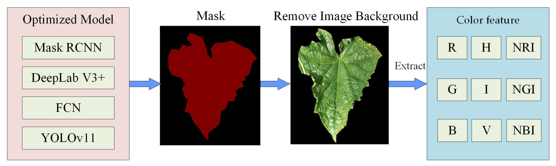
Using the Optimized annotated model, the annotated leaf images were segmented, and the Red (R), Green (G), and Blue (B) values of the background region were suppressed. The R, G, and B values for each pixel within the leaf region were extracted, along with the total pixel count of the leaf area, to calculate the average of R, G, and B values for the entire leaf. The process of color feature extraction for cucumber leaves is illustrated in Figure 5.

Figure 5. Cucumber leaf image segmentation and color feature extraction process.

Following the extraction of R, G, and B features from the 150 Cucumber leaf samples, six additional color features were derived for each leaf based on these primary values: Hue (H), Saturation (S), Brightness (V), Normalized red value (NRI), Normalized green value (NGI), Normalized blue value (NBI). The specific calculation formula is as follows [36]:

$$H=\left\{\begin{array}{ll}0°& if max(r,\mathrm{g},b)=min(r,\mathrm{g},b)\\ \left\{\left[60°\times \left(g-b\right)\right]/\left[max(r,\mathrm{g},b)-min(r,\mathrm{g},b)\right]\right\}+0°,& if r=max(r,\mathrm{g},b) and \mathrm{g}\ge b \\ \left\{\left[60°\times \left(g-b\right)\right]/\left[max(r,\mathrm{g},b)-min(r,\mathrm{g},b)\right]\right\}+360°,& if r=max(r,\mathrm{g},b) and \mathrm{g}<b\\ \left\{\left[60°\times \left(b-r\right)\right]/\left[max(r,\mathrm{g},b)-min(r,\mathrm{g},b)\right]\right\}+120°,& if g=max(r,\mathrm{g},b)\\ \left\{\left[60°\times \left(r-g\right)\right]/\left[max(r,\mathrm{g},b)-min(r,\mathrm{g},b)\right]\right\}+240°,& if b=max(r,\mathrm{g},b)\end{array}\right.$$

(10)

$$l=\left[max(r,g,b)+min(r,g,b)\right]/2$$

(11)

$$S=\left\{\begin{array}{l}0, if l=0 or max(r,g,b)=min(r,g,b)\\ \left[max(r,g,b)-min(r,g,b)\right]/\left[max(r,g,b)+min(r,g,b)\right], if 0<l\le 0.5\\ \left[max(r,g,b)-min(r,g,b)\right]/\left[2-max(r,g,b)-min(r,g,b)\right], if 0.5<l\le 1\end{array}\right.$$

(12)

$$NRI=r/(r+g+b)$$

(13)

$$NGI=g/(r+g+b)$$

(14)

$$NBI=b/(r+g+b)$$

(15)

$$\left\{\begin{array}{l}r=R/255\\ g=G/255\\ b=B/255\end{array}\right.$$

(16)

where $H$ indicates Hue, $\mathrm{g}$ indicates the green light value, $r$ indicates the red light value, $b$ indicates the blue light value, $l$ indicates Saturation, $S$ indicates Brightness, $NRI$ indicates the red light standardization value, $NGI$ indicates the green light standardization value, $NBI$ indicates the standardization value of blue light.

2.4. Intelligent Model for Identifying Nitrogen Fertiliser Content in Cucumber Leaves Based on Colour Characteristics

This study obtained the dry weight, leaf nitrogen content, and nine color feature values from 150 cucumber leaf samples. Given the limited sample size, which is insufficient for training deep learning algorithms, three typical machine learning algorithms were selected to construct a cucumber leaf nitrogen content identification model based on color features: Support Vector Machine (SVM), Random Forest (RF), and Extreme Gradient Boosting (XGBoost).

2.4.1. SVM Architecture and Implementation for Identifying Nitrogen Fertiliser Content

The SVM establishes a hyperplane as the decision surface, thereby maximizing the margin between positive and negative instances [37]. When the kernel function is set to Linear or Radial Basis Function (RBF), the tolerance (Tol) and regularization coefficient (C) are the primary hyperparameters affecting model performance. When the kernel function is set to Polynomial (Poly), the degree of the polynomial (Degree), independent term (Coef0), tolerance (Tol), and regularization coefficient (C) become the main hyperparameters. The linear equation of the hyperplane, the distance formula, and the maximization objective are formulated as follows:

$$y\left(t\right)=w^{T}x+b=0$$

(17)

$${y(w}^{T}x+b)\ge 1$$

(18)

$$d=\left[y(w^{T}x+b)\right]/‖w‖$$

(19)

$$d_{max}=max\left[2\times y(w^{T}x+b)\right]/‖w‖$$

(20)

where w indicates model weight, T indicates transposition, b indicates bias, d indicates distance from the support vector to the hyperplane, and γ indicates maximum distance from the support vector to the hyperplane.

2.4.2. RF Architecture and Implementation for Identifying Nitrogen Fertiliser Content

The Random Forest (RF) algorithm is based on an ensemble of decision trees, where multiple independent trees are constructed using bootstrap aggregating (bagging) with random sampling with replacement from the original dataset. When applied to regression tasks, it essentially functions as a multivariate nonlinear regression model [38]. The final prediction of the model is derived by averaging the outputs of all individual decision trees. The primary hyperparameters affecting the performance of the RF model include the Number of estimators (n_estimators), Maximum tree depth (max_depth), Minimum number of samples required to split an internal node (min_samples_split), and Minimum number of samples required to be at a leaf node (min_samples_leaf).

2.4.3. XGBoost Architecture and Implementation for Identifying Nitrogen Fertiliser Content

The Extreme Gradient Boosting (XGBoost) algorithm is based on the Gradient Boosting Decision Tree (GBDT) framework. It sequentially fits the negative gradient of the loss function from previous trees, and incorporates a second-order Taylor expansion of the loss function to optimize errors, thereby demonstrating superior predictive performance [39]. The primary hyperparameters affecting the performance of XGBoost include the Maximum tree depth (max_depth), Learning rate (eta), Number of estimators (n_estimators), and Subsampling ratio of columns (colsample_bytree). The mathematical formulation of the algorithm is as follows:

$$y_i={\sum }_{n=1}^N{f}_n\left(x_i\right)$$

(21)

$$O\left(\varnothing \right)={\sum }_{i}l\left(y_i,y_j\right)+{\sum }_n\Omega {(f}_n)$$

(22)

$$\Omega {(f}_n)=\gamma T+0.5\lambda {‖\omega ‖}^2$$

(23)

where y_i indicates the predicted value of the i-th sample, x_i indicates the input variable of the i-th sample, f_n indicates prediction function of the n-th decision tree, N indicates Number of decision trees, l(y_i,y_j) indicates Loss function, Ω indicates regularization term, Γ indicates complexity of the model (or penalty for adding a new leaf), T indicates number of leaf nodes, λ indicates regularization coefficient (L2 norm weight), ω indicates weight vector of the leaf nodes (leaf scores).

Based on relevant domestic and international literature and references [40,41,42,43], the hyperparameter ranges for the four neural network architectures were defined, and the number of models trained under different hyperparameter combinations for each network was statistically summarized, with the results presented in Table 1.

Table 1. Statistics of hyperparameter settings and trained model counts for four machine learning models.

Model Type	Hyperparameters	Hyperparameter Settings	Number of Hyperparameters	Number of Trained Models
SVR_Poly	Degree	1, 2, …, 9	9	1764
	Coef0	1 × 10−4, 1 × 10−3, …, 1 × 102	7
	Tol	1 × 10−4, 1 × 10−3, …, 1 × 10−1	4
	C	1 × 10−4, 1 × 10−3, …, 1 × 102	7
SVR_RBF	Tol	1 × 10−4, 1 × 10−3, …, 1 × 10−1	4	72
	C	1 × 10−9, 1 × 10−8, …, 1 × 108	18
RF	N-estimators	1, 2, …, 200	200	100,000
	Max_depth	1, 2, …, 20	20
	Min_samples_split	1, 2, …, 5	5
	Min_samples_leaf	1, 2, …, 5	5
XCBoost	Max_depth	1, 2, …, 10	10	39,800
	Learning Rate	1 × 10−4, 1 × 10−3, …, 1 × 10−1	4
	N_estimators	10, 20, …, 1990	199
	Colsample_bytree	0.5, 0.6, …, 0.9	5

The inputs of the four machine learning models are nine color feature values of cucumber leaves, with the leaf nitrogen content serving as the output of the models. The number of samples in the training set and test set is 120 and 30, respectively. The development tools and training environment of this program are consistent with those of the aforementioned leaf segmentation model.

The trained neural network adopts root mean square error (RMSE), mean absolute error (MAE) and mean square error (MSE) as evaluation indexes, and its calculation formula is as follows:

$$RMSE=\sqrt{{\displaystyle \frac{1}{N}}{\sum }_{i=1}^N{\left(Y_i-X_i\right)}^2}$$

(24)

$$MAE={\displaystyle \frac{1}{N}}{\sum }_{i=1}^N\left|Y_i-X_i\right|$$

(25)

$$MSE={\displaystyle \frac{1}{N}}\sum _{i=1}^N{\left(Y_i-X_i\right)}^2$$

(26)

where N—total number of samples; Yi—the predicted value of the model; Xi—true value.

3. Results

3.1. Comparison of Training Process, Performance and Segmentation Effect of Eight Models for Cucumber Leaf Segmentation at Different Resolutions and with Complex Backgrounds

3.1.1. Comparison of Training Process and Performance of Four Models for Cucumber Leaf Segmentation

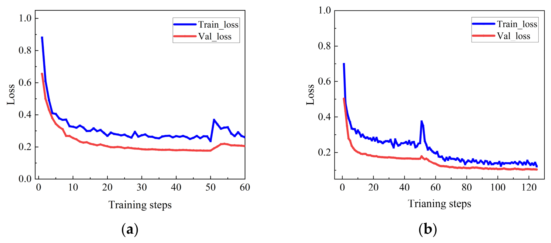
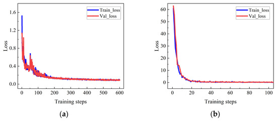
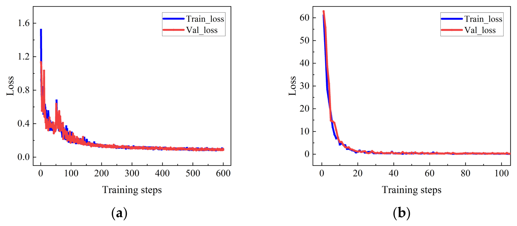
The training of the DeepLab v3+ model for cucumber leaf segmentation against complex backgrounds consists of a freezing phase and an unfreezing phase. Figure 6 shows the evolution of the loss during the training of the DeepLab v3+ model, whose backbone network is MobileNet v2. The figure shows that during the first 50 freezing training epochs, the model’s loss decreases rapidly. After the 10th training epoch, the loss for both the training and validation sets gradually stabilizes, with the training set loss slightly exceeding that of the validation set. During the unfreezing training phase, both the training and validation set losses show a transient increase, then rapidly decrease to the stable level of the freezing phase until training is terminated. To further optimize the model’s segmentation performance, the total number of training epochs was set to 300. The model completed the 50-epoch freezing phase training as scheduled. After 10 training epochs in the unfreezing phase, the model automatically terminated training. Therefore, this paper verifies the accuracy and applicability of the DeepLab v3+ segmentation model based on MobileNet v2.

Figure 6. Loss variation during the training process of the DeepLab v3+ segmentation model. (a) Loss variation of DeepLab v3+ based on MobileNetV2; (b) loss variation of DeepLab v3+ based on Xception.

The changes in loss value during the training process of the DeepLab v3+ model with Xception as the backbone network are shown in Figure 6. It can be seen from the figure that during the first 10 training epochs in the freezing stage, the loss value of the model drops rapidly. During the 10th to 50th training epochs, the loss values for the training set and the validation set both gradually decrease, and the training set loss is greater than the validation set loss. During the unfreezing phase, both the training and validation set losses increase. From the 50th to the 60th training epoch, the model loss continues to decrease. After the 60th epoch, the model loss maintains a slight downward trend, and the gap between the training and validation set losses gradually narrows. After the 80th training epoch, the loss values for both the training and validation sets remain relatively stable. Throughout the training process, the training set loss fluctuates significantly across epochs, while the validation set loss shows minimal fluctuation and maintains a consistent downward trend.

Figure 7a shows the variation in loss during the training of the Mask R-CNN model. During the first 50 training epochs, only the network head (including the RPN, classification/regression branch, and mask branch) is trained with the backbone network frozen. During this process, the loss values for the training and validation sets decrease rapidly, while the loss values for both the training and validation sets fluctuate significantly. Upon entering the unfreezing phase (starting from the 50th epoch), the loss values for both the training and validation sets first show a transient increase. From the 50th to the 100th training epoch, the loss values for both the training and validation sets show a rapid downward trend, with moderate fluctuations that are typical during the parameter fine-tuning period of the unfreezing phase. The loss values for both the training and validation sets do not stabilize until after the 200th training epoch.

Figure 7. Loss variation during the training process of the segmentation model. (a) Loss variation of Mask R-CNN; (b) loss variation of FCN.

Figure 7b shows the changes in loss during the training process of the FCN model with the VGG19 backbone network. As can be seen, during the first 21 training epochs, the loss values for both the training and validation sets show a rapid downward trend. After the 21st training epoch, the loss values for both the training and validation sets tend to stabilize at around 0.2–0.3, indicating successful convergence.

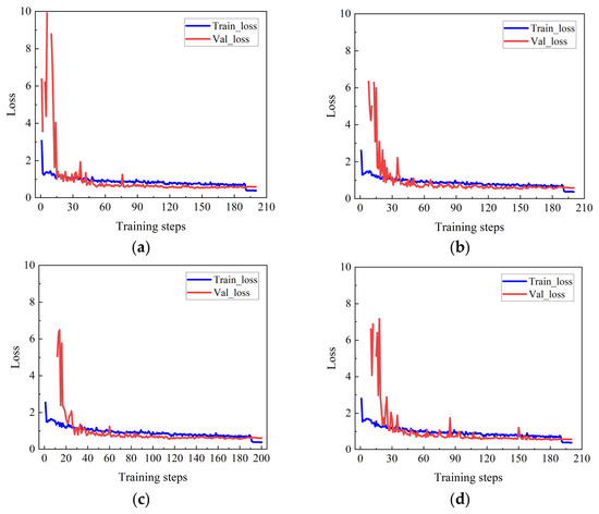
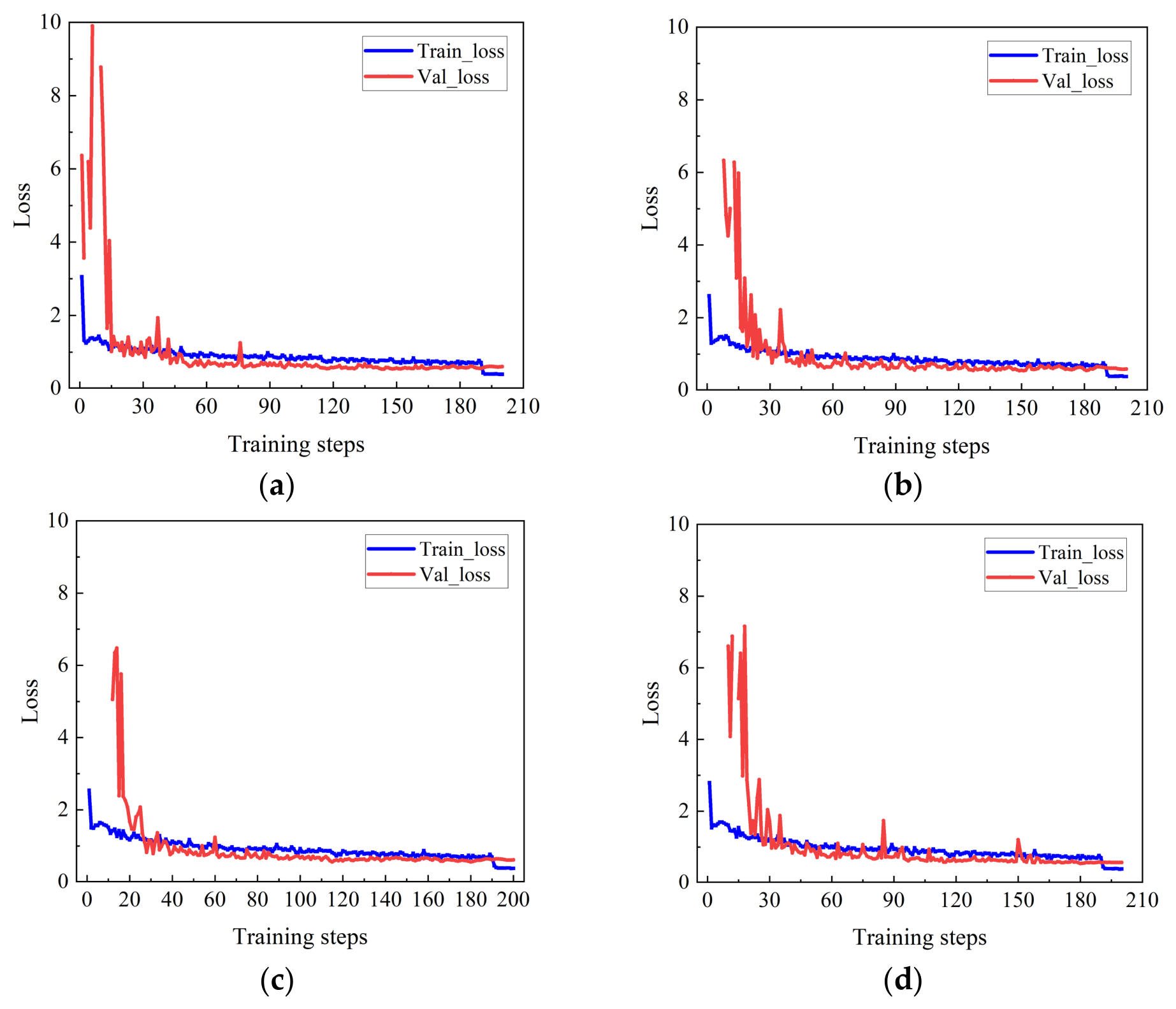
The changes in loss value during the training process of four YOLOv11 models are shown in Figure 8. It can be seen from the figure that during the first 30 training epochs in the freezing stage, the loss value of the model drops rapidly. During the 30th to 200th training epochs, the loss values for the training set and the validation set both gradually decrease, and the validation set loss is greater than the training set loss. After the 30th training epoch, the loss values for both the training and validation sets remain relatively stable. Throughout the training process, the validation set loss fluctuates significantly across epochs, while the training set loss shows minimal fluctuation and maintains a consistent downward trend. The four YOLOv11 segmentation models exhibit consistent trends in loss variation throughout the training process. Furthermore, after 200 training epochs, the discrepancy in dataset scale between the training and test sets remains negligible.

Figure 8. Results of segmenting cucumber leaf images using four YOLOv11 models. (a) Loss variation of YOLOv11n; (b) loss variation of YOLOv11s; (c) loss variation of YOLOv11m; (d) loss variation of YOLOv11l.

Based on the above training results of the eight cucumber leaf image segmentation models (DeepLab v3+, Mask R-CNN, FCN, and YOLOv11), this paper summarizes the performance of the models in terms of training steps, training time, and model storage size. This study evaluates the performance of the models by analyzing their convergence epochs, computational training time, and memory footprints, as shown in Table 2. It can be clearly observed from the data that the YOLOv11n model equipped with the CSPDarknet64, C3k2 and C2PSA backbone network has the shortest total training time, taking only 10 min to complete the full training process, while the standard Mask R-CNN model based on the Faster R-CNN framework has the longest training duration, reaching up to 566 min, which is more than 56.6 times that of the fastest YOLOv11n model. In terms of model storage footprint, the Mask R-CNN model exhibits the largest storage footprint of 245 MB, whereas the YOLOv11n model is the most lightweight, with a size of only 6.0 MB.

Table 2. Training duration and model size of eight segmentation models.

Model Type	Backbone Network	Training Steps	Training Duration (min)	Model Size (MB)
DeepLab v3+_1	MobileNet v2	62	13	10.9
DeepLab v3+_1	Xception	126	63	158
Mask R-CNN	Faster R-CNN	600	566	245
FCN	VGG19	600	128	76.6
YOLOv11n	CSPDarknet64 + C3k2 + C2PSA	200	10	6.0
YOLOv11s		200	11	20.5
YOLOv11m		200	18	45.2
YOLOv11l		200	21	55.9

The results further show that the lightweight design of the backbone network significantly reduces both training time and model size, while the more complex instance segmentation architecture of Mask R-CNN, though delivering higher segmentation accuracy, comes with the cost of longer training cycles and larger storage requirements, which should be considered for practical deployment scenarios. Moreover, the YOLOv11 model demonstrates significant advantages by virtue of its shorter training time and compact model size. Consequently, the optimized DeepLab v3, Mask R-CNN, FCN, and YOLOv11n models were employed to perform segmentation on complex cucumber leaf imagery, facilitating a comprehensive assessment of their performance under challenging agricultural conditions.

3.1.2. Comparison of Segmentation Performance of Five Models for Cucumber Leaves at Different Resolutions and with Complex Backgrounds

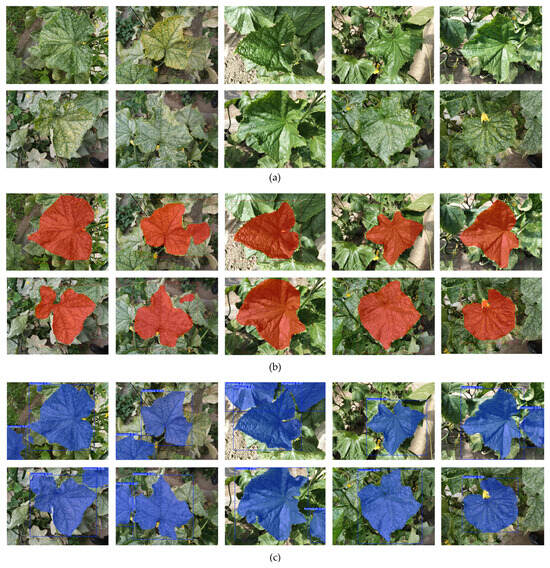
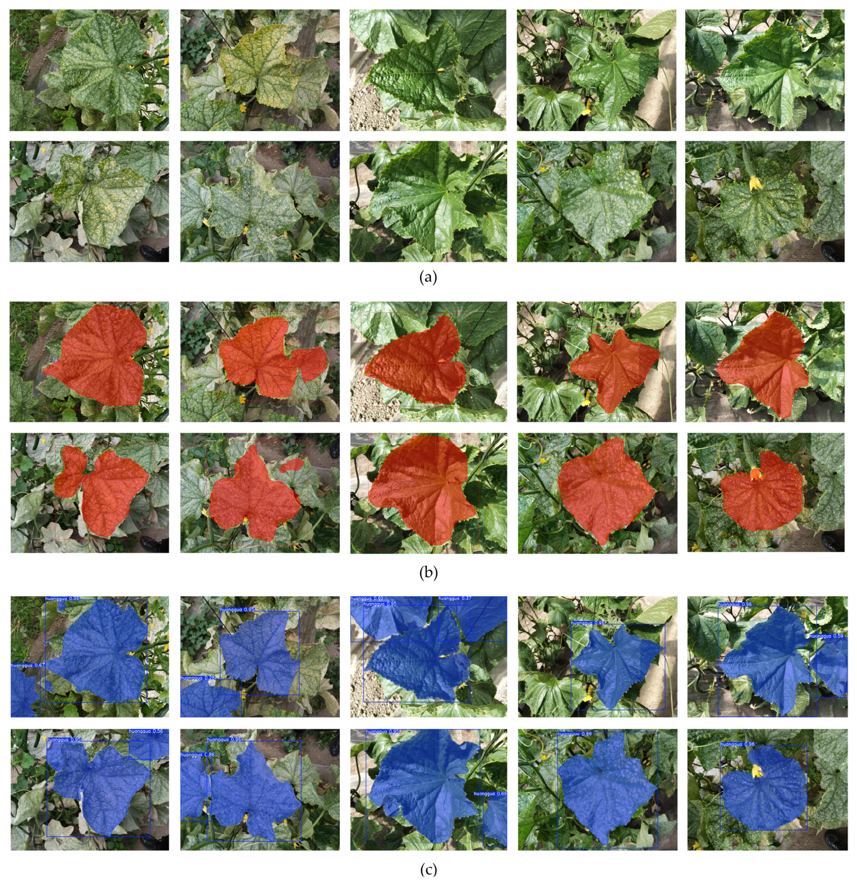
To compare the segmentation performance of the optimized DeepLab v3+, Mask R-CNN, FCN, and YOLOv11n on cucumber leaves with different resolutions and complex backgrounds, 10 cucumber leaf images containing branches, overlapping leaves, and soil were selected, as shown in Figure 9a. The original images had a resolution of 4080 × 3060 pixels and were compressed to generate cucumber leaf images with a resolution of 400 × 300 pixels. In order to verify the segmentation performance of the models on cucumber leaf images with different resolutions, five optimized models were used to segment cucumber leaf images at two different resolutions, and the time required to segment the 10 images was calculated. The average segmentation time for the five models at different cucumber leaf resolutions is shown in Table 3. For a given model, the time consumed for segmenting cucumber leaf images at the two different resolutions showed negligible variation. Mask R-CNN had the longest segmentation time of 34.0 s, while YOLOv11n had the shortest time of 0.053 s. A processing speed of approximately 0.053 s per image is highly suitable for practical fertilization decision-making applications.

Figure 9. Results of segmenting cucumber leaf images with complex backgrounds using optimized models. (a) Images of cucumber leaves; (b) Mask RCNN; (c) YOLOv11n.

Table 3. Average time for segmenting cucumber leaf images at different resolutions.

Model Type	4080 × 3060 Pixels (s)	400 × 300 Pixels (s)
DeepLab v3+_1	16.56	15.22
DeepLab v3+_2	16.40	16.00
Mask R-CNN	34.00	30.90
FCN	28.60	26.24
YOLOv11 n	0.053	0.052

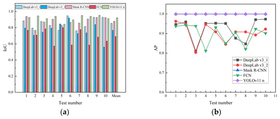
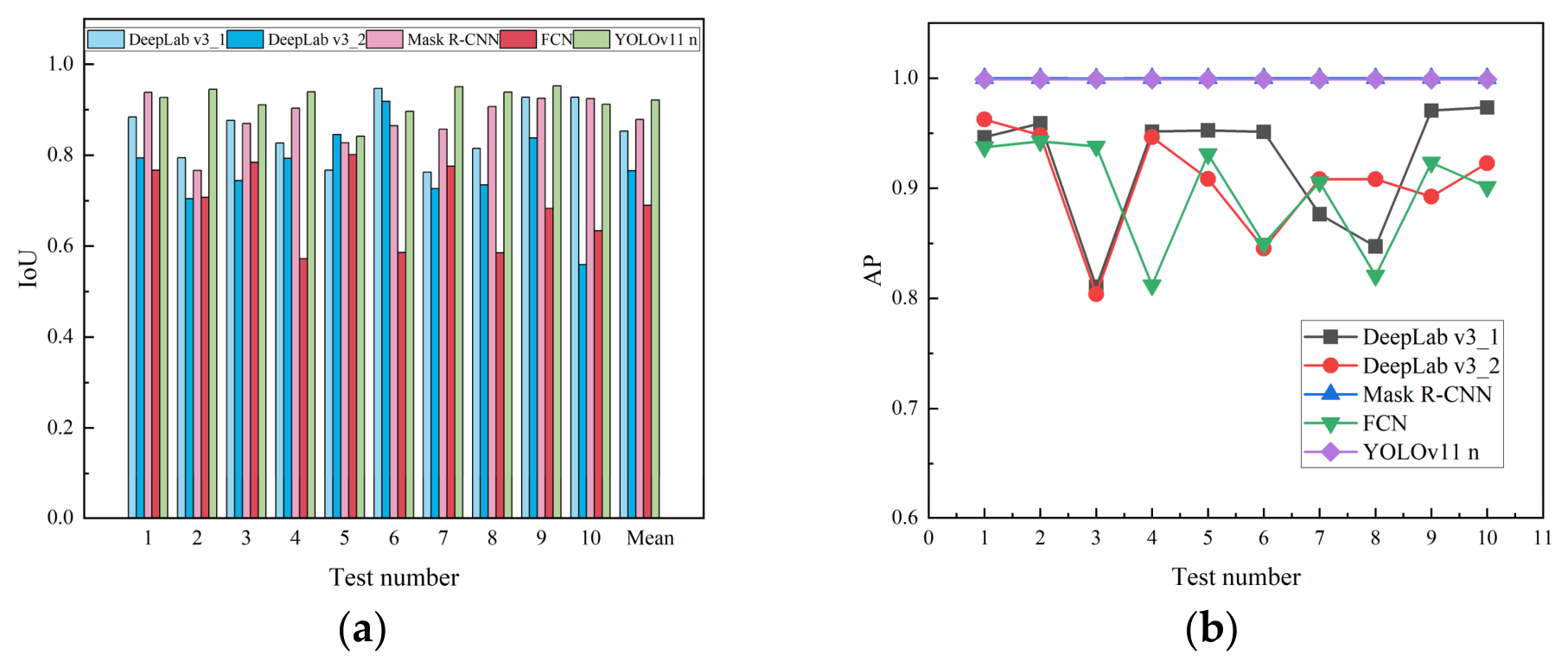
As shown in Figure 10a, among the five segmentation models, the average IoU values in descending order are 0.9212, 0.8784, 0.8528, 0.7657, and 0.6896, corresponding to YOLOv11n, Mask R-CNN, DeepLab v3+_1, DeepLab v3+_2, and FCN respectively. As shown in Figure 10b, the average AP values in descending order are 0.9999, 0.9998, 0.9239, 0.9046, and 0.8960, corresponding to YOLOv11n, Mask R-CNN, DeepLab v3+_1, DeepLab v3+_2, and FCN, respectively. This indicates that the IoU and AP values of the YOLOv11n model are the highest among the five models.

Figure 10. Results of segmenting cucumber leaf images using five models. (a) Result of IoU; (b) Result of AP.

Based on the IoU, mAP, and average segmentation time of the five models, Mask R-CNN and YOLOv11n are identified as the two best-performing models. Therefore, this study employs the optimized Mask R-CNN and YOLOv11n models to segment ten cucumber leaf images against complex backgrounds, with the segmentation results presented in Figure 9. The results indicate that both models can effectively segment cucumber leaf images in complex scenarios; however, YOLOv11n demonstrates the capability to segment partially incomplete leaves, indicating its superior segmentation robustness and providing technical support for the efficient acquisition of leaf color features.

3.2. Determination Results of Nitrogen Fertilizer Content in Cucumber Leaves

3.2.1. Distribution Characteristics and Variation Patterns of Dry Weight and Nitrogen Content of 150 Cucumber Leaves

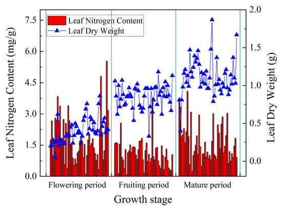
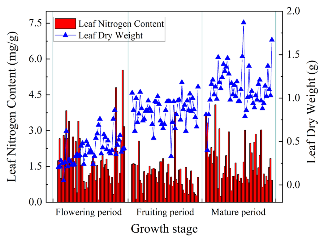
The dry weight and nitrogen content of 150 cucumber leaves were measured, and the results are shown in Figure 11. For the three growth stages, the maximum dry weight of cucumber leaves was 0.86, 1.18, and 1.87 g, respectively, while the corresponding average dry weight was 0.40, 0.85, and 1.11 g, respectively, and the minimum dry weight was 0.05, 0.33, and 0.40 g, respectively. Therefore, the dry weight of cucumber leaves in the flowering stage was relatively small, while that in the fruiting stage was relatively high.

Figure 11. Dry weight and nitrogen content of 150 cucumber leaves at different growth stages.

For the three growth stages, the maximum nitrogen content of cucumber leaves was 3.77, 4.09, and 8.54 mg·g⁻¹, respectively, while the corresponding average nitrogen content was 1.83, 1.10, and 1.64 mg·g⁻¹, respectively, and the minimum nitrogen content was 0.10, 0.08, and 0.25 mg·g⁻¹, respectively. Contrary to the trend of dry weight, the nitrogen content of cucumber leaves was higher in the flowering stage and lower in the mature stage. The main reason is that nitrogen fertilizer is allocated to the growth of cucumber fruits during the mature stage, resulting in a decrease in nitrogen content in the leaves.

3.2.2. Statistical Analysis of Color Features of 150 Cucumber Leaves Based on RGB and HSI Color Spaces

Cucumber leaf images were segmented to remove background information, and nine color feature values for 150 cucumber leaf regions were obtained using the formula mentioned above. Partial data and statistical results are presented in Table 4. As shown in the table, the average green light value of cucumber leaves is higher than both the red light value and the blue light value, and the maximum and minimum green light values of cucumber leaves also exceed the corresponding red and blue light values. The standard deviations of the red light value, green light value, blue light value, and their three corresponding standardized values show no significant difference.

Table 4. Nine color feature values and statistics of 150 cucumber leaf image regions.

No.	r	g	b	h	l	s	NRI	NGI	NBI
1	0.50	0.55	0.35	72.90	0.45	0.23	0.36	0.39	0.25
2	0.45	0.56	0.29	84.57	0.43	0.31	0.35	0.43	0.22
3	0.43	0.52	0.32	86.59	0.42	0.24	0.34	0.41	0.25
4	0.33	0.44	0.20	86.86	0.32	0.38	0.34	0.46	0.20
5	0.45	0.59	0.29	88.97	0.44	0.33	0.34	0.44	0.22
6	0.43	0.55	0.36	95.95	0.45	0.21	0.32	0.41	0.27
7	0.39	0.49	0.29	88.91	0.39	0.25	0.34	0.42	0.25
8	0.33	0.46	0.25	95.90	0.35	0.30	0.32	0.44	0.24
9	0.35	0.46	0.21	87.51	0.34	0.37	0.34	0.45	0.21
10	0.50	0.55	0.35	72.90	0.45	0.23	0.36	0.39	0.25
…	…	…	…	…	…	…	…	…	…
148	0.46	0.58	0.36	93.71	0.47	0.24	0.33	0.42	0.26
149	0.46	0.58	0.37	95.31	0.48	0.22	0.32	0.41	0.26
150	0.39	0.55	0.32	101.03	0.44	0.27	0.31	0.44	0.25
Mean	0.35	0.46	0.23	88.21	0.34	0.37	0.34	0.45	0.21
Max	0.58	0.70	0.47	105.99	0.57	0.68	0.38	0.52	0.29
Min	0.13	0.18	0.05	72.90	0.11	0.16	0.29	0.39	0.10
Standard Deviation	0.12	0.14	0.12	6.16	0.13	0.13	0.02	0.03	0.05
Correlation	−0.043	−0.036	−0.090	−0.126	−0.059	0.109	0.096	0.112	−0.101

Hue refers to the appearance of color, with a variation range of 0–360. In this study, the hue values of cucumber leaves are distributed within the range of 49.3–107.58, exhibiting small variations. Since color information is mainly extracted from the leaf area, and the color variation range of cucumber leaf region images is narrow, the amplitude of hue value changes is also small. The color saturation of cucumber leaves varies within the range of 0.11–0.67, and the brightness (value) varies within the range of 0.06–0.68. The standard deviations of these two features are 0.13 and 0.14, respectively, indicating that the dispersion of saturation and brightness data is not high.

The correlation between the nine color characteristic values and leaf nitrogen content was calculated using IBM SPSS Statistics 20.0 software; the correlation coefficients between the nine color features and leaf nitrogen content ranged from −0.126 to 0.109. The results show that hue, brightness, standardized red light value, standardized green light value, and standardized blue light value have a high correlation with cucumber leaf nitrogen content, while red light value, green light value, and saturation show a low correlation with cucumber leaf nitrogen content.

3.3. Intelligent Recognition Results and Analysis of Nitrogen Fertilizer Content in Cucumber Leaves Based on Color Features

Using 120 sets of cucumber leaf color feature datasets, four machine learning models constructed with different hyperparameters were trained. A total of 30 sets of cucumber leaf color feature datasets were used as the test set, and MSE was used as the evaluation index to compare the predictive performance of the models under each hyperparameter combination.

The best hyperparameters under the minimum MSE of the four machine learning models were obtained, as shown in Table 5. According to the table, the best-to-worst predictive performance of the four machine learning models was in the following order: XGBoost, SVR_Poly, RF, and SVR_RBF, indicating that the optimized XGBoost model has the highest accuracy in identifying nitrogen fertilizer content in cucumber leaves. The MAE, MSE, and RMSE of the predicted values of the XGBoost model are the worst compared to the performance of SVR_RBF. The MAE, MSE, and RMSE of the model are 10.15%, 8.71%, and 4.36% lower, respectively.

Table 5. Optimal Hyperparameters and Prediction Errors of Four Machine Learning Models.

Model Type	Hyperparameters	Hyperparameter Settings	MAE	MSE	RMSE
SVR_Poly	Degree	5	0.504	0.482	0.695
	Coef0	1
	Tol	100
	C	0.1
SVR_RBF	Tol	100	0.522	0.505	0.710
	C	0.1
RF	N-estimators	20	0.520	0.458	0.677
	Max_depth	11
	Min_samples_split	2
	Min_samples_leaf	2
XCBoost	Max_depth	2	0.469	0.461	0.679
	Learning Rate	0.1
	N_estimators	20
	Colsample_bytree	0.7

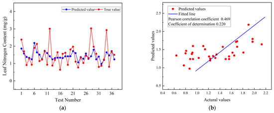
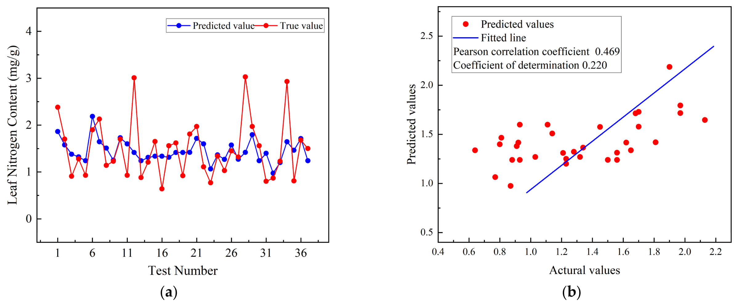
Based on the nine color feature values of the leaf region, the optimal XGBoost model was used to predict the nitrogen content of 37 cucumber leaves. The comparison between the predicted values and the true values is shown in Figure 12. It can be seen from the figure that the nitrogen content of the 37 cucumber leaves is distributed in the range of 0.5 to 3.5 mg·g⁻¹. The nitrogen content predicted by the XGBoost model is mostly distributed in the range of 1.0 to 2.5 mg·g⁻¹. The overall nitrogen content predicted by the model is lower than the true value, indicating that the optimized model can predict the nitrogen content of cucumber leaves relatively well. The prediction results show a Pearson’s r of 0.46949 and an R² of only 0.22042, indicating a moderate correlation between predicted and true values, with only 22% of nitrogen content variation explained by the model. This aligns with the XGBoost model’s MAE of 0.469 in the document. The overall prediction trend roughly matches the true values, but there is still room for accuracy improvement.

Figure 12. The prediction performance of the optimized model. (a) Ground Truth and XGBoost Model Predicted Values of Cucumber Leaf Nitrogen Content; (b) Fitted curve of predicted vs. measured values.

4. Discussion

This study systematically evaluated the performance of five mainstream deep learning segmentation models—including Mask R-CNN, DeepLab v3+ equipped with MobileNet v2 and Xception backbones, FCN with a VGG19 backbone, and YOLOv11n—on cucumber leaf segmentation tasks under complex background conditions.

The results indicate that YOLOv11n achieved the optimal overall segmentation accuracy: for high-resolution 4080 × 3060 images, its IoU reached 0.9212 and AP reached 0.9999, significantly outperforming the DeepLab v3+ series and FCN models. This study also revealed the limitations of Mask R-CNN in terms of segmentation efficiency: its single-image segmentation time was approximately 34 s, and its model size was 245 MB, metrics far inferior to those of the lightweight DeepLab v3+ (which requires only 13 min for training, occupies 10.9 MB of storage space, and achieves an inference speed of 16 frames per second).

In contrast, Zhang et al. proposed the optimized CL-YOLO v8 model [27], introducing a Multi-Scale Feature Module (MSFM) to replace the bottleneck structure of the original C2f module, embedding an Efficient Multi-scale Attention (EMA) mechanism to enhance illumination robustness, and designing an Efficient Sub-Pixel Upsampling Block (ESPUB). While that model achieved a segmentation mAP@50 of 0.914, the optimized YOLOv11n model in this study attained an mAP@50 of 0.999, surpassing the aforementioned model. This demonstrates that the optimized model in this paper exhibits significant accuracy advantages and is more suitable for real-time monitoring on embedded devices in plant factories.

The hyperspectral and Raman spectroscopy instruments are characterized by high costs and poor adaptability to complex field environments, which makes them difficult to deploy on a large scale at cultivation sites. In contrast, this study relies solely on conventional optical imaging equipment for image acquisition. By integrating a pre-trained YOLOv11n segmentation model with a lightweight XGBoost prediction model, the proposed scheme not only features low hardware costs but is also more suitable for routine precision fertilization management of greenhouse cucumbers.

However, the current study is limited to indoor validation using static images, and the model’s performance under extreme natural lighting conditions requires further verification. To bridge this gap, future work will focus on deploying the lightweight model on mobile edge devices (e.g., smartphones or portable terminals) for real-time, on-site testing. Additionally, we plan to expand the dataset to encompass more diverse growth stages and cucumber varieties to enhance the model’s generalization capability.

5. Conclusions

A systematic evaluation of eight mainstream deep learning segmentation models under complex background conditions demonstrates that the standard YOLOv11n model achieves optimal instance segmentation accuracy for cucumber leaves without targeted structural improvements. For high-resolution images, it attained an IoU of 0.9212 and an AP of 0.9998, significantly outperforming the DeepLab v3+ series and FCN models. Furthermore, YOLOv11n exhibits significant advantages in segmentation efficiency (0.053 s/image) and model size (6.0 MB) compared to Mask R-CNN (34 s/image, 245 MB).

Based on color features extracted from leaf regions segmented by YOLOv11n, the optimized XGBoost model achieved the best performance for nitrogen content prediction, yielding an MAE of 0.469, an MSE of 0.461, and an RMSE of 0.679. This outperformed the SVR-Poly, RF, and SVR-RBF models. Furthermore, the predicted nitrogen values aligned closely with the distribution trend of the ground truth values, thereby verifying the feasibility of the proposed pipeline: deep learning segmentation—color feature extraction—machine learning prediction.

In contrast to high-cost hyperspectral and Raman spectroscopy technologies, which are often difficult to deploy in field environments, the proposed scheme relies solely on conventional optical imaging equipment. By integrating a pre-trained Mask R-CNN segmentation model with a lightweight XGBoost prediction model, the system offers low hardware costs and is highly suitable for routine precision fertilization management in greenhouse cucumber cultivation.

References

- Ayoub Shaikh, T.; Rasool, T.; Rasheed Lone, F. Towards leveraging the role of machine learning and artificial intelligence in precision agriculture and smart farming. Comput. Electron. Agric. 2022, 198, 107119. [Google Scholar] [CrossRef] [Scilit]
- Bwambale, E.; Abagale, F.K.; Anornu, G.K. Smart irrigation monitoring and control strategies for improving water use efficiency in precision agriculture: A review. Agric. Water Manag. 2022, 260, 107324. [Google Scholar] [CrossRef] [Scilit]
- Ghazal, S.; Munir, A.; Qureshi, W.S. Computer vision in smart agriculture and precision farming: Techniques and applications. Artif. Intell. Agric. 2024, 13, 64–83. [Google Scholar] [CrossRef] [Scilit]
- Zhao, H.; Zhai, X.; Guo, L.; Yang, Y.; Li, J.; Ren, C.; Wang, K.; Liu, X.; Zhan, R.; Wang, K. Comparing protected cucumber and field cucumber production systems in China based on emergy analysis. J. Clean. Prod. 2019, 236, 117648. [Google Scholar] [CrossRef] [Scilit]
- Li, W.; Zhang, W.; Wei, R.; Liu, Z.; Liu, X. Innovative Substrate Design for Sustainable Agriculture: Kitchen Compost and Organic Waste in Cucumber Seedling Cultivation. Pol. J. Environ. Stud. 2025, 3497–3508. [Google Scholar] [CrossRef] [Scilit] [PubMed]
- Muñoz-Huerta, R.; Guevara-Gonzalez, R.; Contreras-Medina, L.; Torres-Pacheco, I.; Prado-Olivarez, J.; Ocampo-Velazquez, R. A Review of Methods for Sensing the Nitrogen Status in Plants: Advantages, Disadvantages and Recent Advances. Sensors 2013, 13, 10823–10843. [Google Scholar] [CrossRef] [Scilit] [PubMed]
- Rivacoba, L. Nondestructive diagnosis of nitrogen status in cauliflower using a Dualex® leaf-clip sensor: Calibration of an NBI-based critical curve across three seasons. J. Plant Nutr. 2026, 49, 1090–1097. [Google Scholar] [CrossRef] [Scilit]
- Luo, Z.; Yang, W.; Yuan, Y.; Gou, R.; Li, X. Semantic segmentation of agricultural images: A survey. Inf. Process. Agric. 2024, 11, 172–186. [Google Scholar] [CrossRef] [Scilit]
- Raei, E.; Akbari Asanjan, A.; Nikoo, M.R.; Sadegh, M.; Pourshahabi, S.; Adamowski, J.F. A deep learning image segmentation model for agricultural irrigation system classification. Comput. Electron. Agric. 2022, 198, 106977. [Google Scholar] [CrossRef] [Scilit]
- Sabzi, S.; Pourdarbani, R.; Rohban, M.H.; García-Mateos, G.; Paliwal, J.; Molina-Martínez, J.M. Early Detection of Excess Nitrogen Consumption in Cucumber Plants Using Hyperspectral Imaging Based on Hybrid Neural Networks and the Imperialist Competitive Algorithm. Agronomy 2021, 11, 575. [Google Scholar] [CrossRef] [Scilit]
- Hou, Z.; Wang, Y.; Tan, F.; Gao, J.; Jiao, F.; Su, C.; Zheng, X. Selection of Optimal Diagnostic Positions for Early Nutrient Deficiency in Cucumber Leaves Based on Spatial Distribution of Raman Spectra. Plants 2025, 14, 1199. [Google Scholar] [CrossRef] [Scilit] [PubMed]
- Hou, Z.; Tan, F.; Li, M.; Gao, J.; Su, C.; Jiao, F.; Wang, Y.; Zheng, X. Quantitative Determination of Nitrogen Content in Cucumber Leaves Using Raman Spectroscopy and Multidimensional Feature Selection. Agronomy 2025, 15, 1884. [Google Scholar] [CrossRef] [Scilit]
- Chungcharoen, T.; Donis-Gonzalez, I.; Phetpan, K.; Udompetaikul, V.; Sirisomboon, P.; Suwalak, R. Machine learning-based prediction of nutritional status in oil palm leaves using proximal multispectral images. Comput. Electron. Agric. 2022, 198, 107019. [Google Scholar] [CrossRef] [Scilit]
- Cao, L.; Li, H.; Yu, H.; Chen, G.; Wang, H. Plant Leaf Segmentation and Phenotypic Analysis Based on Fully Convolutional Neural Network. Appl. Eng. Agric. 2021, 37, 929–940. [Google Scholar] [CrossRef] [Scilit]
- Liang, J.; Ren, W.; Liu, X.; Zha, H.; Wu, X.; He, C.; Sun, J.; Zhu, M.; Mi, G.; Chen, F.; et al. Improving Nitrogen Status Diagnosis and Recommendation of Maize Using UAV Remote Sensing Data. Agronomy 2023, 13, 1994. [Google Scholar] [CrossRef] [Scilit]
- Xu, T.; Yao, L.; Xu, L.; Chen, Q.; Yang, Z. Image Segmentation of Cucumber Seedlings Based on Genetic Algorithm. Sustainability 2023, 15, 3089. [Google Scholar] [CrossRef] [Scilit]
- Jia, W.; Zhang, Z.; Shao, W.; Hou, S.; Ji, Z.; Liu, G.; Yin, X. FoveaMask: A fast and accurate deep learning model for green fruit instance segmentation. Comput. Electron. Agric. 2021, 191, 106488. [Google Scholar] [CrossRef] [Scilit]
- Qiao, G.F.; Zhang, Z.B.; Niu, B.; Han, S.J.; Yang, E.H. Plant stem and leaf segmentation and phenotypic parameter extraction using neural radiance fields and lightweight point cloud segmentation networks. Front. Plant Sci. 2025, 16, 1170. [Google Scholar] [CrossRef] [Scilit] [PubMed]
- Son, J.-H.; Song, H.; Song, C.-y.; Ha, M.; Kang, D.; Ha, Y.-S. Condition-based synthetic dataset for amodal segmentation of occluded cucumbers in agricultural images. Comput. Electron. Agric. 2025, 238, 110800. [Google Scholar] [CrossRef] [Scilit]
- Liu, L.; Li, G.; Du, Y.; Li, X.; Wu, X.; Qiao, Z.; Wang, T. CS-net: Conv-simpleformer network for agricultural image segmentation. Pattern Recognit. 2024, 147, 110140. [Google Scholar] [CrossRef] [Scilit]
- Wang, D.Y.; Fu, Y.Y.; Yang, G.J.; Yang, X.D.; Liang, D.; Zhou, C.Q.; Zhang, N.; Wu, H.Y.; Zhang, D.Y. Combined Use of FCN and Harris Corner Detection for Counting Wheat Ears in Field Conditions. IEEE Access 2019, 7, 178930–178941. [Google Scholar] [CrossRef] [Scilit]
- Yang, K.; Zhong, W.; Li, F. Leaf Segmentation and Classification with a Complicated Background Using Deep Learning. Agronomy 2020, 10, 1721. [Google Scholar] [CrossRef] [Scilit]
- Yang, T.; Zhou, S.; Xu, A.; Ye, J.; Yin, J. An Approach for Plant Leaf Image Segmentation Based on YOLOV8 and the Improved DEEPLABV3+. Plants 2023, 12, 3438. [Google Scholar] [CrossRef] [Scilit] [PubMed]
- Qian, T.; Liu, Y.; Lu, S.; Li, L.; Zheng, X.; Ju, Q.; Li, Y.; Xie, C.; Li, G. Cucumber Leaf Segmentation Based on Bilayer Convolutional Network. Agronomy 2024, 14, 2664. [Google Scholar] [CrossRef] [Scilit]
- Medentzidis, C.R.; Kapetas, D.; Pechlivani, E.M. Fungal Disease Detection on Vegetable Crops Using RGB Imaging. Agriculture 2026, 16, 541. [Google Scholar] [CrossRef] [Scilit]
- Yao, H.; Wang, C.; Zhang, L.; Li, J.; Liu, B.; Liang, F. A Cucumber Leaf Disease Severity Grading Method in Natural Environment Based on the Fusion of TRNet and U-Net. Agronomy 2023, 14, 72. [Google Scholar] [CrossRef] [Scilit]
- Zhang, D.; Li, N.; Zhao, M.; Xu, K. Improved YOLOv8 Algorithm was Used to Segment Cucumber Seedlings Under Complex Artificial Light Conditions. IEEE Access 2025, 13, 83944–83955. [Google Scholar] [CrossRef] [Scilit]
- Crespo, A.; Moncada, C.; Crespo, F.; Morocho-Cayamcela, M.E. An efficient strawberry segmentation model based on Mask R-CNN and TensorRT. Artif. Intell. Agric. 2025, 15, 327–337. [Google Scholar] [CrossRef] [Scilit]
- Ahmed, M.E.; Pinki, F.T.; Quader, M.A.; Quader, M.A.; Ayrin, F.J.; Anwar, A.S.; Roy, P. Towards Accurate Renal Micro-Structure Segmentation: An Assessment of YOLOv8 and Mask R-CNN Models. In Proceedings of the 2024 IEEE International Women in Engineering (WIE) Conference on Electrical and Computer Engineering (WIECON-ECE), Chennai, India, 6–7 December 2024; pp. 326–331. [Google Scholar]
- Pan, Z.; Zhang, X.; Jiang, Y.; Li, B.; Golsanami, N.; Su, H.; Cai, Y. High-precision segmentation and quantification of tunnel lining crack using an improved DeepLabV3+. Undergr. Space 2025, 22, 96–109. [Google Scholar] [CrossRef] [Scilit]
- Huang, Z.; Pan, Y.; Huang, W.; Pan, F.; Wang, H.; Yan, C.; Ye, R.; Weng, S.; Cai, J.; Li, Y. Predicting Microvascular Invasion and Early Recurrence in Hepatocellular Carcinoma Using DeepLab V3+ Segmentation of Multiregional MR Habitat Images. Acad. Radiol. 2025, 32, 3342–3357. [Google Scholar] [CrossRef] [Scilit] [PubMed]
- Shelhamer, E.; Long, J.; Darrell, T. Fully Convolutional Networks for Semantic Segmentation. IEEE Trans. Pattern Anal. Mach. Intell. 2017, 39, 640–651. [Google Scholar] [CrossRef] [Scilit] [PubMed]
- Alkhammash, E.H. A Comparative Analysis of YOLOv9, YOLOv10, YOLOv11 for Smoke and Fire Detection. Fire 2025, 8, 26. [Google Scholar] [CrossRef] [Scilit]
- Wang, Y.X.; Zhao, J.H.; Xu, H.Y.; Han, C.; Tao, Z.Q.; Zhou, D.W.; Geng, T.; Liu, D.F.; Ji, Z.C. A systematic evaluation of computational methods for cell segmentation. Brief. Bioinform. 2024, 25, bbae407. [Google Scholar] [CrossRef] [Scilit] [PubMed]
- Abro, B.A.; Memon, M.; Zia-Ul, H.; Arain, M.Y.; Razaq, A.; Abro, D.A.; Ali, S. Assessing nitrogen nutrition of banana basrai cultivar (Dwarf Cavendish) through leaf analysis and chlorophyll determination. Pak. J. Bot. 2021, 53, 1859–1864. [Google Scholar] [CrossRef] [Scilit] [PubMed]
- Huang, L.Q.; Zhao, W.B.; Liew, A.W.C.; You, Y. An evidential combination method with multi-color spaces for remote sensing image scene classification. Inf. Fusion 2023, 93, 209–226. [Google Scholar] [CrossRef] [Scilit]
- Wang, Z.X.; Zhang, X.L.; Hu, X.X.; Miao, H.; Zhang, S.J.; Chang, F.; Wei, R.H.; Guo, Z. Establishing and validating a predictive model for long-term control outcomes following orthokeratology lenses wear: A five-year cohort study. Front. Cell Dev. Biol. 2026, 14, 1743506. [Google Scholar] [CrossRef] [Scilit] [PubMed]
- Jia, Z.; Cheng, Z.J.; Chang, Z.L.; Li, Q.; Huang, F.M.; Peng, Y.H. Non-landslide sample for landslide susceptibility prediction modeling: A review of selection strategies and their influence rules. J. Rock Mech. Geotech. Eng. 2026, 18, 2859–2880. [Google Scholar] [CrossRef] [Scilit]
- Sahin, E.K. Implementation of free and open-source semi-automatic feature engineering tool in landslide susceptibility mapping using the machine-learning algorithms RF, SVM, and XGBoost. Stoch. Environ. Res. Risk Assess. 2023, 37, 1067–1092. [Google Scholar] [CrossRef] [Scilit]
- Arbi, S.J.; Rehman, Z.U.; Hassan, W.; Khalid, U.; Ijaz, N.; Maqsood, Z.; Haider, A. Optimized machine learning-based enhanced modeling of pile bearing capacity in layered soils using random and grid search techniques. Earth Sci. Inform. 2025, 18, 332. [Google Scholar] [CrossRef] [Scilit]
- Borgohain, R.; Goswami, G.; Das, J.; Khandai, S.; Tyagi, N.K.; Chakrawarti, N. Explaining grain quality trait importance and classification of traditional rice cultivars of Assam, India using SHAP-enhanced Random Forest, XGBoost, and Support Vector Machine models. J. Cereal Sci. 2026, 129, 104457. [Google Scholar] [CrossRef] [Scilit]
- Khalifani, F.M.; Lentz, D.R.; Walker, J.A. Machine learning-based mineral prospectivity mapping of epithermal gold mineralization in Northern new brunswick: A comparative study of random forest, support vector machine, and XGboost classifiers. Earth Sci. Inform. 2025, 18, 553. [Google Scholar] [CrossRef] [Scilit]
- Qu, X.H.; Jiang, C.; Shan, M.Y.; Ke, W.H.; Chen, J.; Zhao, Q.M.; Hu, Y.H.; Liu, J.; Qin, L.P.; Cheng, G. Prediction of Proteolysis-Targeting Chimeras Retention Time Using XGBoost Model Incorporated with Chromatographic Conditions. J. Chem. Inf. Model. 2025, 65, 613–625. [Google Scholar] [CrossRef] [Scilit] [PubMed]
Disclaimer/Publisher’s Note: The statements, opinions and data contained in all publications are solely those of the individual author(s) and contributor(s) and not of MDPI and/or the editor(s). MDPI and/or the editor(s) disclaim responsibility for any injury to people or property resulting from any ideas, methods, instructions or products referred to in the content. |
© 2026 by the authors. Licensee MDPI, Basel, Switzerland. This article is an open access article distributed under the terms and conditions of the Creative Commons Attribution (CC BY) license.