U-PKAN: A Dual-Module Kolmogorov–Arnold Network for Agricultural Plant Disease Detection

Abstract

Crop diseases and pests have a significant impact on planting costs and crop yields and, in severe cases, can threaten food security and farmers’ incomes. Currently, most researchers employ various deep learning methods, such as the YOLO series algorithms and U-Net and its variants, for the detection of agricultural plant diseases. However, the existing algorithms suffer from insufficient interpretability and are limited to linear modeling, which can lead to issues such as trust crises in current technologies, restricted applications and difficulties in tracing and correcting errors. To address these issues, a dual-module Kolmogorov–Arnold Network (U-PKAN) is proposed for agricultural plant disease detection in this paper. A KAN encoder–decoder structure is adopted to construct the network. To ensure the network fully extracts features, two different modules, namely Patchembed-KAN (P-KAN) and Decoder-KAN (D-KAN), are designed. To enhance the network’s feature fusion capability, a KAN-based symmetrical structure for skip connections is designed. The proposed method places learnable activation functions on weights, enabling it to achieve higher accuracy with fewer parameters. Moreover, it can reveal the compositional structure and variable dependencies of synthetic datasets through symbolic formulas, thus exhibiting excellent interpretability. A field corn disease image dataset was collected and constructed. Additionally, the performance of the U-PKAN model was verified using the open plant disease dataset PlantDoc and a gear pitting dataset. To better understand the performance differences between different methods, U-PKAN was compared with U-KAN, U-Net, AttUNet, and U-Net++ models for performance benchmarking. IoU and the Dice coefficient were chosen as evaluation metrics. The experimental results demonstrate that the proposed method achieves faster convergence and higher segmentation accuracy. Overall, the proposed method demonstrates outstanding performance in aspects such as function approximation, global perception, interpretability and computational efficiency.

1. Introduction

In contemporary society, there is a growing demand for food and an increasing emphasis on quality. However, agricultural production is encountering unprecedented challenges due to severe labor shortages [1]. Intelligent agriculture and digital technology have been used to improve the production efficiency of agriculture. However, crop yield and quality fluctuations persist due to the influences of the natural environment, biological processes and human interference [2]. Among these factors, agricultural plant diseases caused by bacteria, fungi, and pests cause significant annual crop damage. These diseases seriously hinder the growth of crops [3,4]. Therefore, early and accurate detection of these diseases is crucial to prevent crop waste and reduce economic losses.

Traditional agricultural disease detection is heavily dependent on the subjective experience of inspectors, meaning it lacks objectivity [5]. Misdiagnosis or delayed treatment often leads to improper pesticide use, failing to control diseases while damaging crops and the environment [6]. Modern detection technologies have emerged as alternatives. Spectral analysis, with its rich spatial–spectral information, has shown promise in target detection, classification and environmental monitoring [7]. Related studies include hyperspectral sensing [8], multispectral imaging combined with spatial–spectral machine learning [9] and spectral data analysis for identifying plant biomarkers [10]. However, hyperspectral and multispectral technologies are associated with high equipment costs and low acquisition efficiency, making them unsuitable for real-time, large-scale farmland inspections [11,12]. In contrast, deep learning-based methods using CCD cameras offer low hardware costs, millisecond-level imaging speeds and intuitive processing, making them ideal for rapid, large-scale detection [13].

Deep learning (DL) has increasingly been adopted to enhance the accuracy of agricultural disease detection [14,15,16]. For example, the HODRF system combines YOLOv7 (object detection) and EfficientNetV2 (classification) to improve diagnostic performance [17]. While the YOLO series algorithms excel at the rapid localization of infected regions, they struggle with low accuracy in complex environments and with small targets, and cannot quantify disease infection rates (i.e., the ratio of diseased to healthy leaf areas). In contrast, image segmentation technologies enable pixel-level classification of disease regions, precisely outlining lesion contours and calculating infection rates through pixel statistics—providing critical support for dynamic pest monitoring and precise control decisions.

U-Net and its variants have become mainstream segmentation frameworks for plant disease detection, leveraging U-shaped architectures and skip connections to integrate local details and global semantic information [18,19,20,21]. However, their practical application in agricultural scenarios is constrained by two critical issues that are exacerbated by the inherent complexity of field agricultural images. Field images typically exhibit strong illumination variations, low-contrast textures and irregular lesion shapes, which result in blurred lesion boundaries and fragmented diseased regions. Conventional U-Net-based models struggle to capture these fine-grained textures and often misidentify lesion edges, leading to poor segmentation accuracy for ambiguous targets [22]. Additionally, most U-Net variants rely on fixed nonlinear activation functions. This not only restricts their ability to model complex nonlinear interactions in dynamic field conditions but also reinforces the "black-box" nature of the models, which reduces interpretability and complicates error tracing and correction [23]. These combined limitations highlight the urgent need for an architecture that jointly enhances interpretability, boundary segmentation precision and robustness to noisy field environments, addressing the reliability gaps of existing methods in practical agricultural applications.

The emergence of Kolmogorov–Arnold Networks (KANs) has addressed some of these issues [24]. KANs decompose complex multivariate functions into combinations of univariate functions and binary additions, enabling more accurate function approximation with fewer parameters than traditional "black-box" neural networks [25]. With the development of KANs, many researchers have proposed models that integrate KANs into neural networks [26]. U-KAN, a hybrid architecture integrating KANs into U-Net [27], has achieved good results in medical image segmentation. A. D. Bodner et al. [28] proposed a novel neural network architecture called CKAN. It builds a completely new kind of layer by integrating the nonlinear activation function in KANs into the convolution operation. The purpose is to improve the expression ability of the model, reduce the number of parameters and improve the optimization efficiency. M. Cheon et al. [29] improved efficiency and performance by combining a KAN with the ConvNeXt algorithm. This ensures the model performs well in remote sensing image classification tasks. M. Cheon [30] proposed KCN, a method that combines KANs with various pre-trained convolutional neural network models for remote sensing scene classification tasks. T. B. Ayaz et al. [31] used edge-conditional convolution (ECC) and a graphical autoencoder built using KANs to exploit the graphical representation of business process traces. To improve the model built using Multilayer Perceptron (MLP) as the decoder, M. M. Ferdaus et al. [32] proposed the compact variant KANice-mini. This model maintains comparable performance with KANice while reducing the number of parameters. Through comprehensive experimental evaluation and ablation studies, its superior performance on multiple image classification tasks is verified via comprehensive experiments and ablation studies. An optimized KAN encoder and a spatial–spectral KAN encoder were designed by Y. Wang et al. [33] These encoders reduce the number of parameters and computational complexity and better handle high-dimensional data. The study also discusses its future application in multi-modal data fusion and time series analysis. Despite these advances in KAN models, related research is still in the development stage. The models’ long-term stability and reliability in complex mission scenarios have not been fully verified, which limits their widespread application in real production environments.

Therefore, in order to develop a suitable model for agricultural plant disease detection, a dual-module Kolmogorov–Arnold Network (U-PKAN) is proposed for agricultural plant disease detection. The contributions of this paper are summarized as follows:

(1)

A more accurate and interpretable agricultural plant disease detection model is proposed that boasts stronger function representation capability and avoids the problem of catastrophic forgetting. Through tests on both self-built and public datasets, the model achieved the best performance across multiple metrics.

(2)

A novel encoder–decoder architecture (U-PKAN) is developed. The proposed method, based on the Kolmogorov–Arnold representation theorem, decomposes complex high-dimensional functions into combinations of simple one-dimensional functions. It enhances approximation accuracy by refining the grids of internal spline functions. By visualizing activation functions to identify potential symbolic representations and understand the model’s decision-making process, the method exhibits high computational efficiency and excellent interpretability.

(3)

A dual-module architecture (P-KAN and D-KAN) is designed. In P-KAN, the extracted features are transformed into sequence samples with positional information, thereby achieving dependency modeling of long-distance information. In D-KAN, interpolation is fused with KAN to unify the resolution of features at different levels, and the computational efficiency is optimized through a "coarse-to-fine" strategy.

2. Materials and Methods

2.1. U-PKAN Network Structure

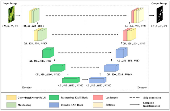
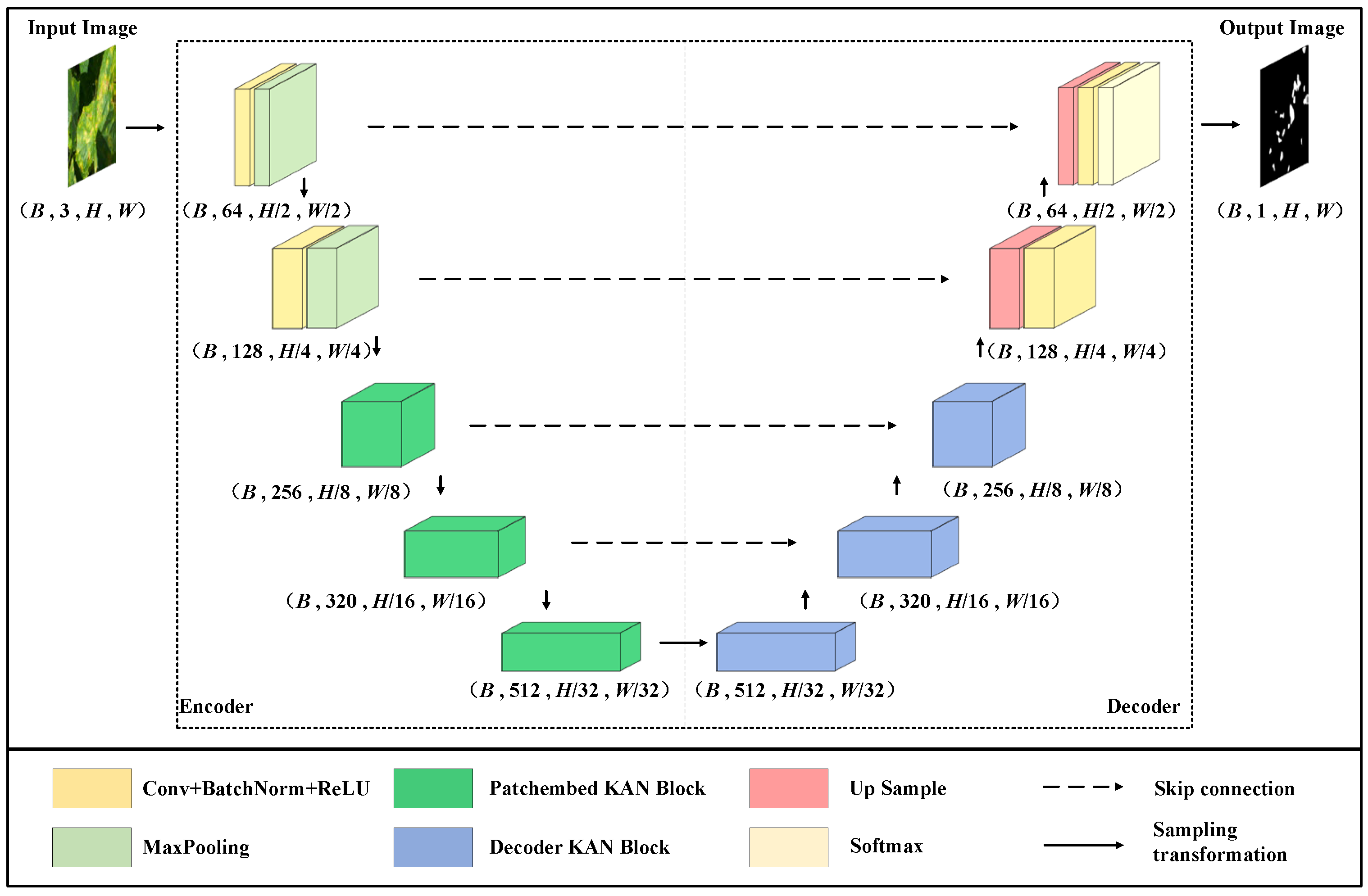
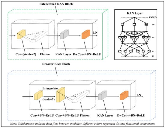
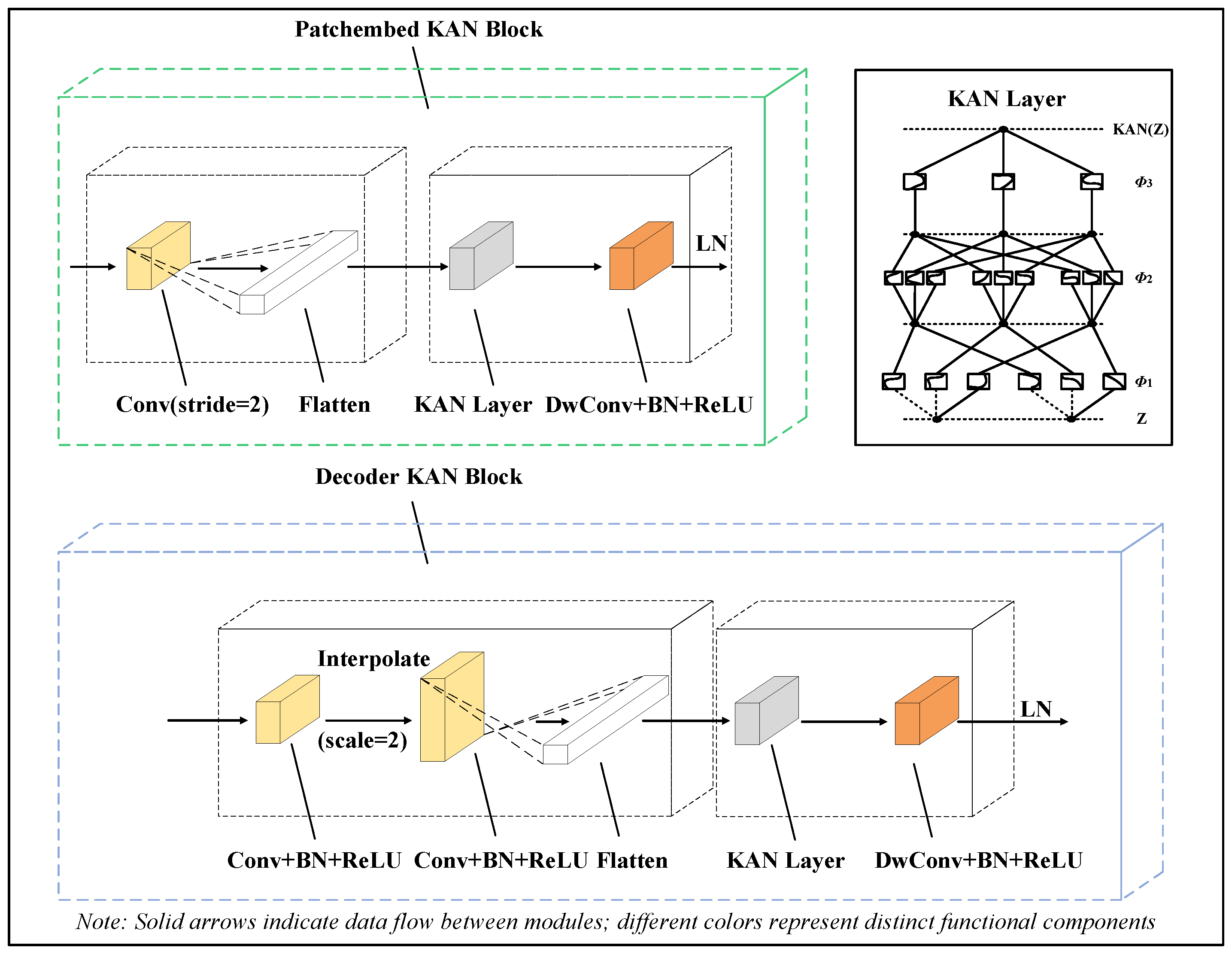
The overall proposed network structure is shown in Figure 1. The overall structure of the encoder–decoder is presented, which includes the convolutional block, Patchembed-KAN block and Decoder-KAN block. The structures of the P-KAN and D-KAN blocks are shown in Figure 2. The encoder consists of two convolutional blocks and three P-KAN blocks, and the decoder consists of three D-KAN blocks and two convolutional blocks. After the original image is input, the input x is extracted to perform encoding, bottleneck processing and decoding operations in sequence. In the encoding stage, the image features are gradually extracted and compressed by convolution and P-KAN block, and the intermediate features are saved. Subsequently, the features are further transformed through the bottleneck layer. At the decoding stage, the upsampling is performed by the D-KAN block and the convolutional block, whereas the features saved in the encoding stage are added. The image resolution is restored by upsampling combined with different feature levels, and the final output is the processed result. The simplified architecture diagram is shown in Table 1. In order to better describe the structure, the U-PKAN algorithm is shown in Table 2.

Figure 1. U-PKAN structure.

Figure 2. The structures of the P-KAN and D-KAN blocks.

Table 1. Simplified architecture block diagram.

Network Stage	Module Type	Kernel Size	Parameter Count (k)	Feature Resolution Change
Encoder 1	Convolution Block	3 × 3	1.792	256 × 256 → 128 × 128
Encoder 2	P-KAN Block	-	8.192	128 × 128 → 64 × 64
Encoder 3	P-KAN Block	-	16.384	64 × 64 → 32 × 32
Encoder 4	P-KAN Block	-	32.768	32 × 32 → 16 × 16
Bottleneck	Conv	3 × 3	65.536	16 × 16 → 8 × 8
Decoder 1	D-KAN Block	-	32.768	8 × 8 → 16 × 16
Decoder 2	D-KAN Block	-	16.384	16 × 16 → 32 × 32
Decoder 3	D-KAN Block	-	8.192	32 × 32 → 64 × 64
Output Layer	1 × 1 Conv	1 × 1	0.513	64 × 64 → 256 × 256

Table 2. U-PKAN algorithm.

Algorithm: U-PKAN Image Segmentation
Input: Image $X_0\in {ℝ}^{B\times C_0\times H_0\times W_0}$, NEncoder, NDecoder
Output: Segmentation result $X^{\prime }\in {ℝ}^{B\times C_0\times H_0\times W_0}$
Encoding: For i = 1 to NEncoder:
I ← ConvBlock(I)
I ← Patchembed KAN Block(I)
Save Ii
Decoding: For j = NDecoder downto 1:
Z ← Upsample(Z)
Z ← Z + Ij
Z ← Decoder KAN Block(Z)
Z ← ConvBlock(Z)
Output: $X^{\prime }$ ← Softmax(Conv1 × 1(Z))
Return $X^{\prime }$

2.2. The Convolution Block in U-PKAN

Each convolutional block consists of a convolutional layer, a batch normalization layer and a ReLU activation function. The convolution kernel size of the convolutional layer is 3 × 3 and the step size is 1. Activation and Maxpooling are carried out after every convolution block; the step size of the Maxpooling layer is 2. The input image can be expressed as $X_0\in {ℝ}^{B\times C_0\times H_0\times W_0}$. The output result of each convolutional block is

$$X_{\mathcal{l}}=\mathrm{MaxPool}\left(\sigma \left(\mathrm{BN}\left({\mathrm{W}}_1\ast X_{\mathcal{l}-1}\right)\right)\right),$$

(1)

where * is the convolution operation, $\sigma$ is the ReLU activation function, $X_{\mathcal{l}}\in {ℝ}^{B\times C_0\times H_0\times W_0}$ represents the output feature map of the $\mathcal{l}$-th layer, L is the number in the convolution module and the final output is X_L. X_L denotes the output feature map of the L-th layer in the convolution block, which is an intermediate feature of local texture extraction with gradually changing dimensions during convolutional operations. In contrast, X’ in Table 2 represents the final segmentation result map output by the model, with the same resolution as the input image and used for pixel-level disease region classification.

2.3. The Patchembed KAN Block in U-PKAN

In this module, the feature map X_L output from the convolution part is used as the input to perform the patch embedding operation through Patchembed, and its spatial dimension is divided to realize the block effect. The channel dimension of the feature map is changed by setting the appropriate number of convolution kernel channels. Here, the number of input channels of the convolution kernel is the number of channels Cin of the input feature map, the convolution projection is performed on the channel dimension and for each output position (B, H, W) is calculated on the channel dimension.

Key parameters of the P-KAN module are specified as follows:

Convolutional projection: 64 kernels with a stride of 1; kernel size = patch size (P_h = 4, P_w = 4).

KAN layer: Uniform grid partitioning strategy (grid size = 10); learnable spline activation functions (cubic B-spline basis functions).

Dimensionality transformation: Flatten (B, C, H × W) → Transpose (B, H × W, C); prioritizes positional information preservation by retaining spatial index mapping.

After convolution projection, the feature map Z_L undergoes flattening (B, C, H × W) and transpose (B, H × W, C) operations to retain positional information and is then input to a three-layer KAN. Features are subsequently processed via a depth-wise convolutional layer (DwConv, kernel size 3 × 3) and layer normalization (LN) to facilitate feature propagation.

The results of the KAN from layer k to layer k + 1 can be represented in matrix form ${\mathrm{Z}}_{k+1}={\Phi }_k{\mathrm{Z}}_k$, where

$${\Phi }_k=\left(\begin{array}{cccc}{\varphi }_{k,1,1\left(\cdot \right)}& {\varphi }_{k,1,2\left(\cdot \right)}& \dots & {\varphi }_{k,1,n_k\left(\cdot \right)}\\ {\varphi }_{k,2,1\left(\cdot \right)}& {\varphi }_{k,2,2\left(\cdot \right)}& \dots & {\varphi }_{k,2,n_k\left(\cdot \right)}\\ ⋮& ⋮& & ⋮\\ {\varphi }_{k,n_{k+1},1\left(\cdot \right)}& {\varphi }_{k,n_{k+1},2\left(\cdot \right)}& \dots & {\varphi }_{k,n_{k+1},n_k\left(\cdot \right)}\end{array}\right)$$

(2)

The K KAN layer here can be described as a nesting of multiple KAN layers as follows:

$$\mathrm{KAN}\left(Z\right)=\left({\Phi }_{K-1}\circ {\Phi }_{K-2}\circ \cdots \circ {\Phi }_0\left(Z\right)\right),$$

(3)

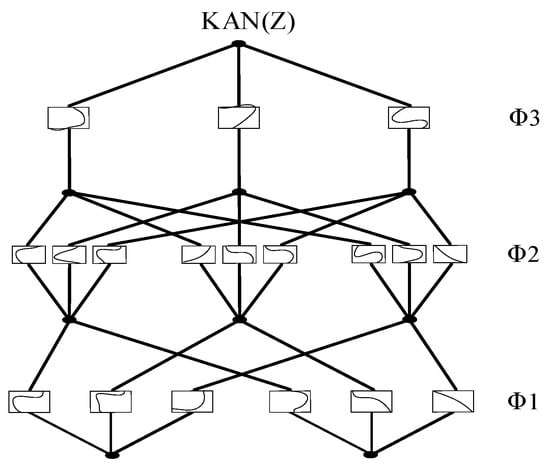
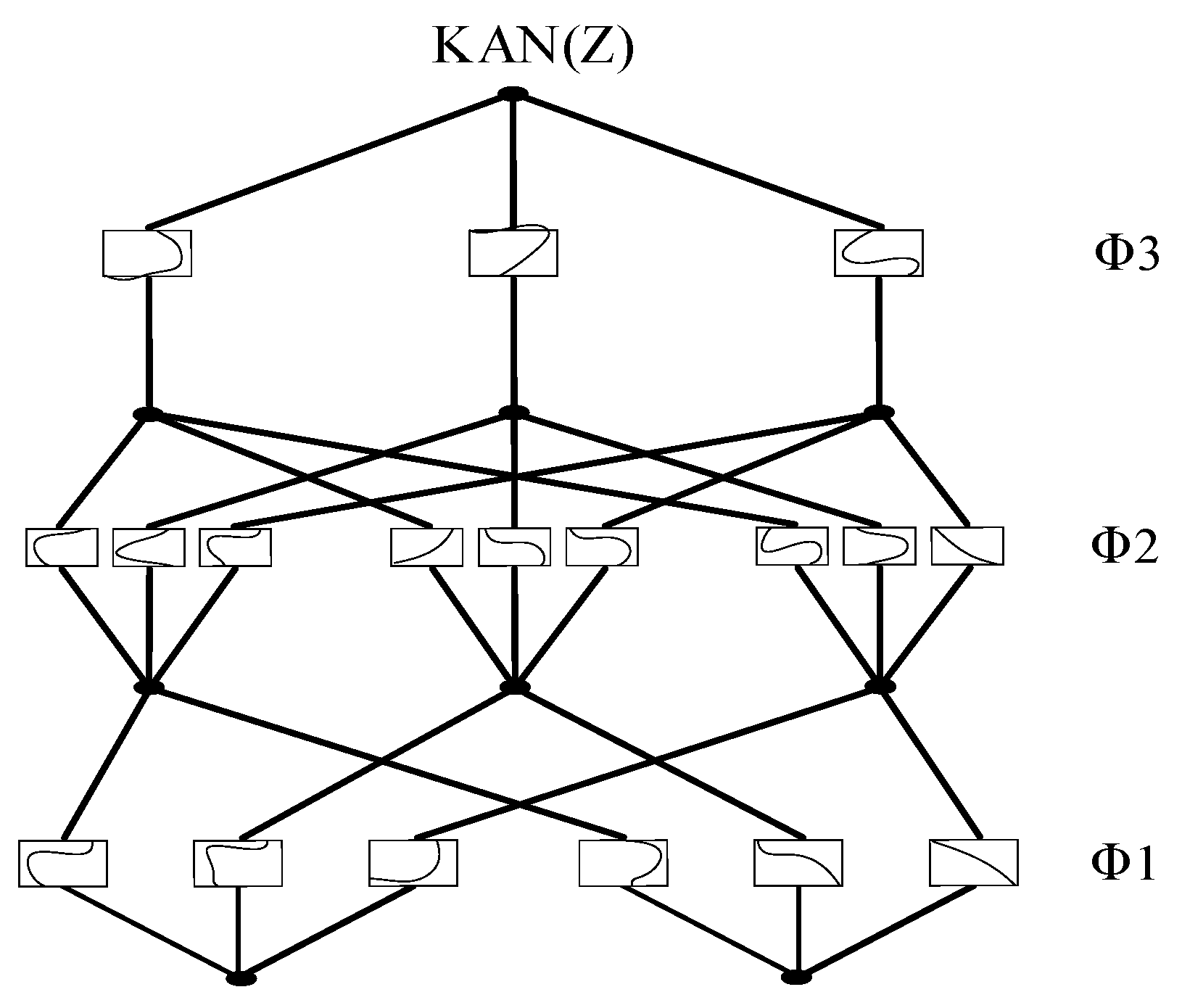
The KAN layer architecture is shown in Figure 3, where ${\Phi }_i$ represents the i-th layer of the entire KAN. For each KAN layer with n_in dimensional input and n_out dimensional output, Φ contains $n_{in} \times n_{out}$ learnable activation functions $\varphi$

$$\Phi =\left\{{\varphi }_{q,p}\right\},p=1,2,\cdots ,n_{in},q=1,2,\cdots ,n_{out},$$

(4)

Figure 3. KAN layer structure.

After the KAN layer, the features are passed through an efficient deep convolutional layer (DwConv). A layer normalization (LN) is then applied to move the features through the next module. This P-KAN module can be elaborated as follows

$$Z_k=\mathrm{LN}\left(\sigma \left(\mathrm{BN}\left(\mathrm{DwConv}\left(\mathrm{KAN}\left(Z_{k-1}\right)\right)\right)\right)\right),$$

(5)

where the feature map of Z_k is (H_k, W_k, C_k). The number k of P-KAN blocks is set to 3.

2.4. The Decoder KAN Block in U-PKAN

Dense skip connections are employed in U-PKAN for low-level detail recovery, and an encoder–decoder structure is adopted for feature extraction.

The key parameters of the D-KAN module are as follows:

Interpolation method: Bilinear interpolation (to ensure smooth upsampling of feature maps without introducing excessive noise).

Fusion weight allocation: Dynamic ratio (initial weight: interpolation = 0.3, KAN = 0.7; adaptively adjusted via backpropagation).

Coarse-to-fine feature conversion threshold: Feature variance threshold = 0.1; when the variance of the fused feature map is greater than 0.1 (indicating coarse feature distribution with large differences), the model adopts fine-grained fusion (increasing the number of KAN grid points to 15); when the variance is less than or equal to 0.1 (indicating uniform feature distribution), coarse-grained fusion is used (grid points = 10) to balance accuracy and computational efficiency.

Upsampled features (from bottleneck) are fused with encoder-preserved features via element-wise addition. The fused features are processed via a KAN layer, DwConv (kernel size 3 × 3) and LN to unify feature resolution, ensuring consistency for the subsequent decoding stages.

2.5. Loss Function in U-PKAN

The loss function is shown in the following equation. The class weight w is added to the Cross Entropy (CE) loss function. That is, the original cross-entropy loss is weighted according to the weight w_y corresponding to the target class y:

$$L_{seg}=-w_y\log \left({\stackrel{⌢}{p}}_y\right),$$

(6)

After the above loss function, the final segmentation map $X_0^{\prime }$ (H₀ × W₀ × C_y) can be output, where C_y is the number of semantic categories.

3. Results

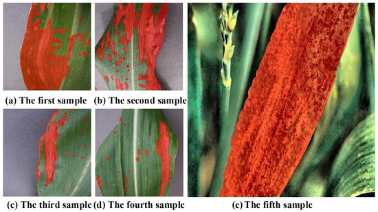
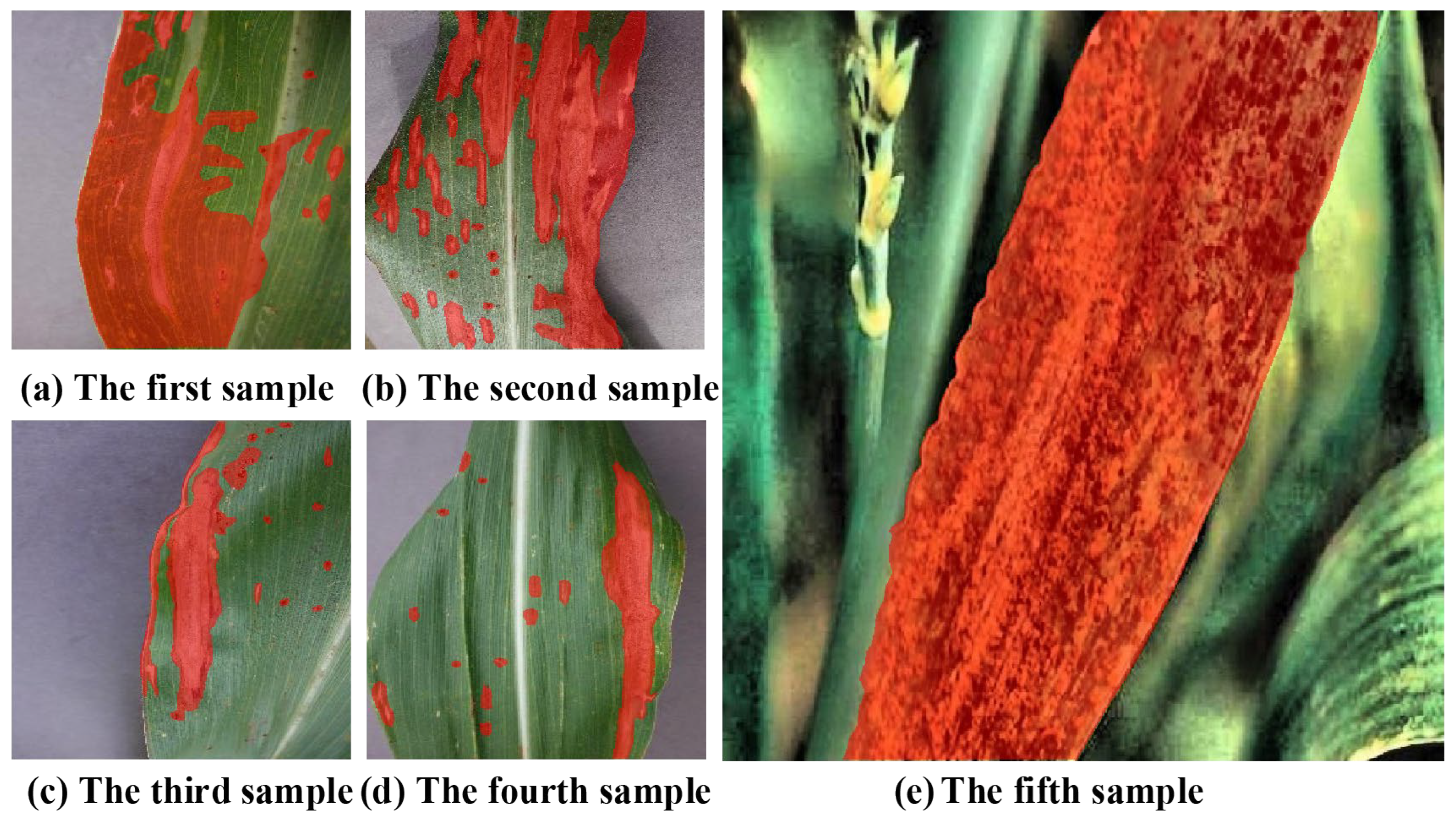
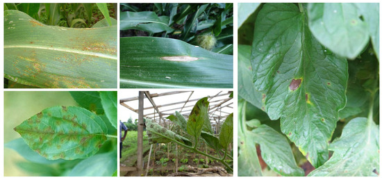
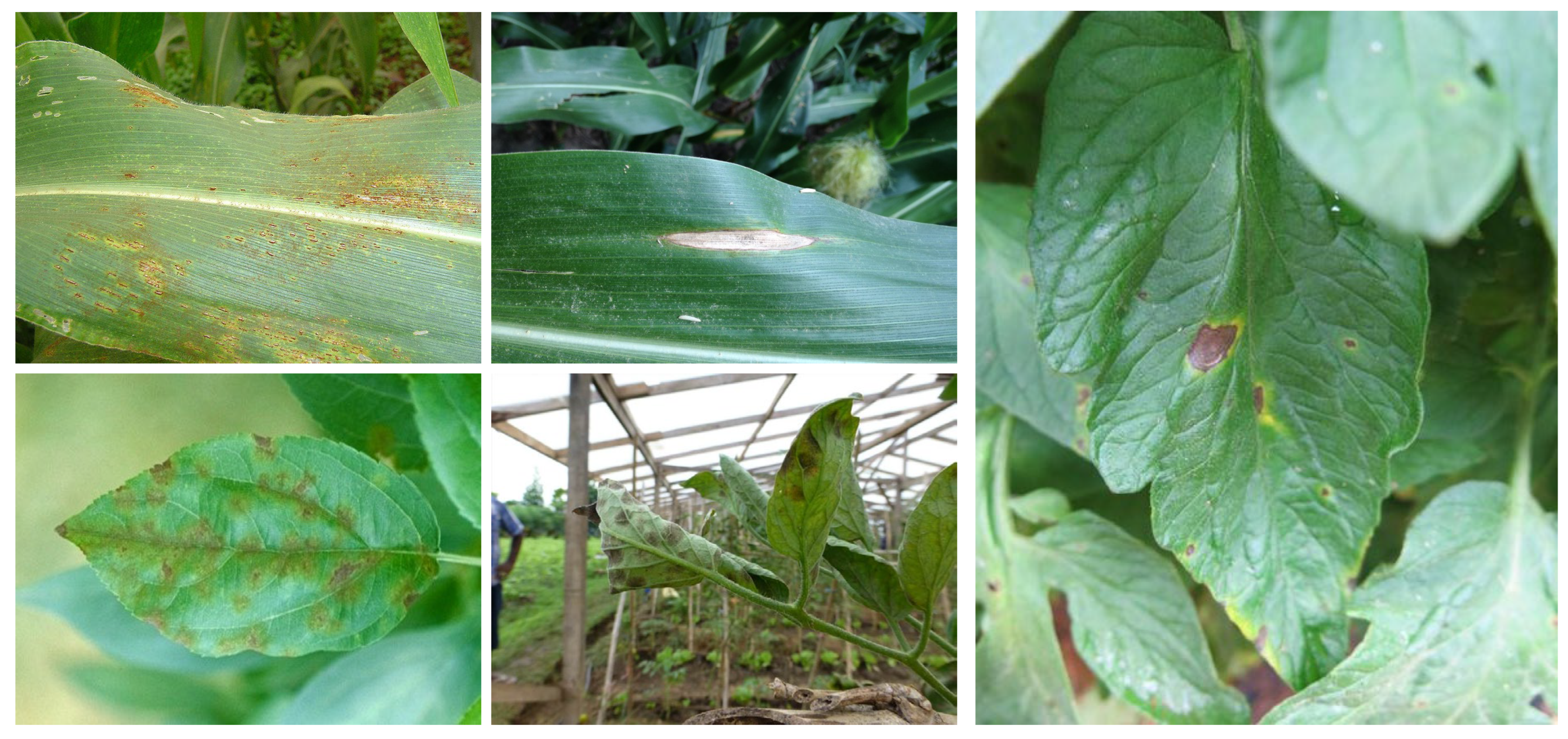
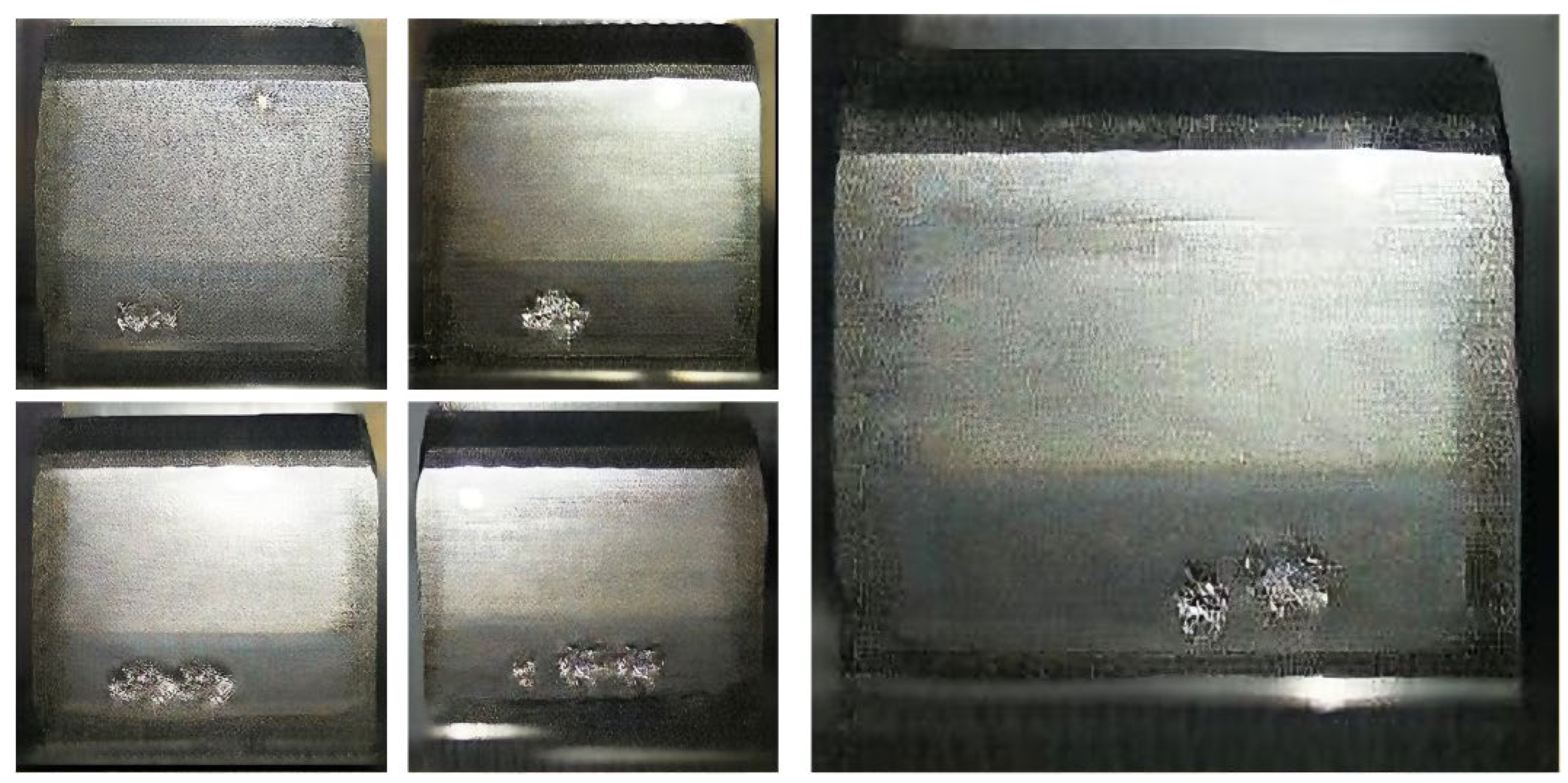
Dataset: Agricultural plant disease images and gear pitting images have similar textures and fuzzy boundaries. Therefore, the dataset used in this paper consists of three parts: a self-built dataset, the publicly available agricultural plant disease dataset PlantDoc and a dataset of gear pitting images [34]. The disease images in the self-built dataset were collected in the corn planting area of the Smart Agriculture Experimental Park of Northeast Agricultural University. The plant diseases captured included corn leaf spot disease, corn gray leaf spot disease, corn mosaic disease and corn rust disease. Due to the complexity of the corn growth environment, different lighting conditions and various other characteristics can affect image quality. During the picture-taking process, diverse imaging strategies (front lighting, back lighting, and angle adjustment) were adopted to enhance data diversity and enhance the model’s generalization ability. All indoor experiments were conducted under controlled environmental conditions: light intensity 8000 ± 500 lx (white LED light source), temperature 25 ± 2 °C, relative humidity 50% ± 5% and no wind interference. These controlled variables ensure the stability and reproducibility of the experimental results. To ensure consistency across different environments, all annotations were conducted by experienced plant experts. These experts used labelme (v5.1.1, MIT Computer Science and Artificial Intelligence Laboratory, Cambridge, MA, USA) to meticulously annotate all disease areas in the corn leaf dataset. Their precise annotation of challenging instances provided important data support and enabled efficient model training. Some annotated samples are shown in Figure 4. The specific characteristics of the self-built corn leaf disease dataset are summarized in Table 3. The publicly available PlantDoc agricultural plant disease image dataset contains different image resolutions for each picture. The dataset contains 504 images of diseased leaves and 504 corresponding mask images. The image content includes plant diseases such as apple scab, apple rust, leaf spot disease, corn leaf blight and potato early blight. Specific information regarding the dataset is shown in Table 4. Example images from the PlantDoc dataset are shown in Figure 5 (including examples of five difference diseases, including apple black spot disease and corn big spot disease). The gear pitting image dataset is used to test the proposed method and is suitable for image segmentation. The dataset contains 814 gear pitting images, and the input resolution of each image is 256 × 256. Specific information regarding the dataset is presented in Table 5. Example images from the gear pitting dataset are shown in Figure 6 (images depicting different degrees of gear pitting are included).

Figure 4. Partially labeled samples from self-built dataset.

Table 3. Corn leaf disease image dataset.

Dataset	Total Number of Images	Train	Validation
Corn leaf diseases	1330	1064	266

Table 4. PlantDoc image dataset.

Dataset	Total Number of Images	Train	Validation
PlantDoc	504	403	101

Figure 5. Sample images from the PlantDoc dataset.

Table 5. Gear pitting image dataset.

Dataset	Input Resolution	Total Number of Images	Train	Validation
Gear Pitting	256 × 256	814	651	163

Figure 6. Sample images from the gear pitting dataset.

Implementation Details: Experiments related to U-PKAN were conducted using Pytorch (v2.0.1, Meta Platforms, Inc., Menlo Park, CA, USA) on an NVIDIA RTX 4090D GPU (NVIDIA Corporation, Santa Clara, CA, USA). For three image datasets, the initial learning rate is set to 0.0001, and the batch size is set to 8. The model is trained using the Adam optimizer and the cosine annealing learning rate scheduler with a minimum learning rate of 0.00001. The loss function uses the above cross-entropy loss formula considering class weights. In this paper, IoU [35] and the Dice coefficient [36] are selected to evaluate the performance of the segmentation model. Moreover, the dataset is randomly split into 80% training and 20% validation. These datasets are averaged over multiple training runs, with data augmentation including 90-degree rotation, horizontal flipping, and image scaling. Training epochs are set based on dataset complexity: 400 epochs for the self-built and PlantDoc datasets (more diverse lesion types and complex backgrounds require longer training to converge) and 50 epochs for the gear pitting dataset (uniform image resolution and simple texture features lead to faster convergence).

3.1. Ablation Experiments

In order to thoroughly verify the model architecture and performance impact in different settings, we first performed the ablation test in the following manner. It has previously been demonstrated that KANs are able to model finer segmentation details by explicitly incorporating efficient embeddings. The effect of the model on the segmentation performance of agricultural plant disease images is evaluated by varying the number of KAN layers; three, four, and five KAN layers were chosen for comparison experiments. The experimental results are shown in Table 6, where it can be observed that the three-layer KAN yields the best performance. The feature extraction and fusion capabilities of the P-KAN and D-KAN modules proposed in this paper have also been fully verified.

Table 6. KAN layer ablation experiments.

KAN	IoU ↑	Dice ↑
3 Layer	94.97	97.42
4 Layer	94.81	97.33
5 Layer	94.74	97.29

In order to test the influence of different numbers of the two designed modules on segmentation accuracy, two, three, and four blocks of the modules were used. The U-PKAN model was used for comparative experiments. As shown in Table 7, the best performance was achieved when three modules were used in the model. This configuration improved the segmentation ability of the network model to a certain extent, as it was associated with superior segmentation performance.

Table 7. KAN block ablation tests.

KAN Block Number	IoU	Dice
KAN Block × 2	94.85	97.36
KAN Block × 3	94.97	97.42
KAN Block × 4	94.56	97.20

3.2. Comparison of the Convergence Performance of Different Models

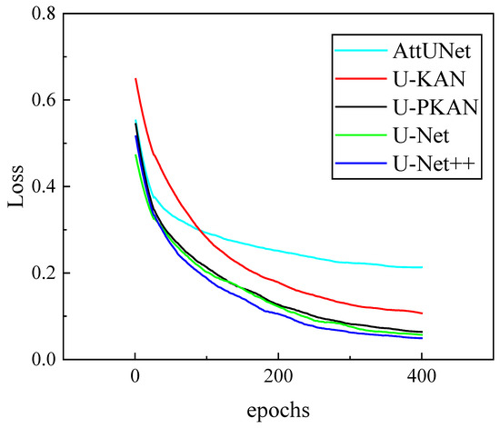
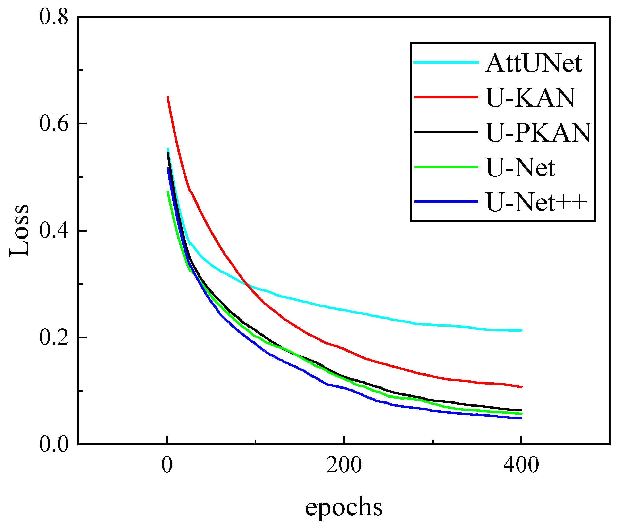
After the ablation experiment verification, a three-layer KAN structure was adopted, and the number of P-KAN and D-KAN modules was set to three. In order to better verify the segmentation ability of U-PKAN, comparative experiments were performed. Firstly, a comparative experiment was carried out on the self-constructed dataset using U-PKAN, U-Net, U-Net++, AttUNet and U-KAN. The loss curves are presented in Figure 7. At the initial stage, the AttUNet loss value was approximately between 0.55 and 0.6. As the number of epochs increased to 200, the loss value dropped to approximately 0.25. When the number of epochs reached 400, the loss value was close to 0.2. This indicates that the decline was significant in the early stages and then slowed down. The initial loss value of U-KAN was about 0.65 − 0.7. When the number of epochs was 200, the loss value had decreased to approximately 0.15; at 400 epochs, the loss value was slightly above 0.1. The decline of U-KAN was rapid in the early stages and slow in the later stages, while the final loss value was relatively higher than that in other models. The downward trends of U-PKAN, U-Net and U-Net++ were stable, and their final loss values were similar.

Figure 7. Loss functions of different models on self-built dataset.

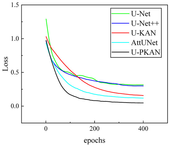
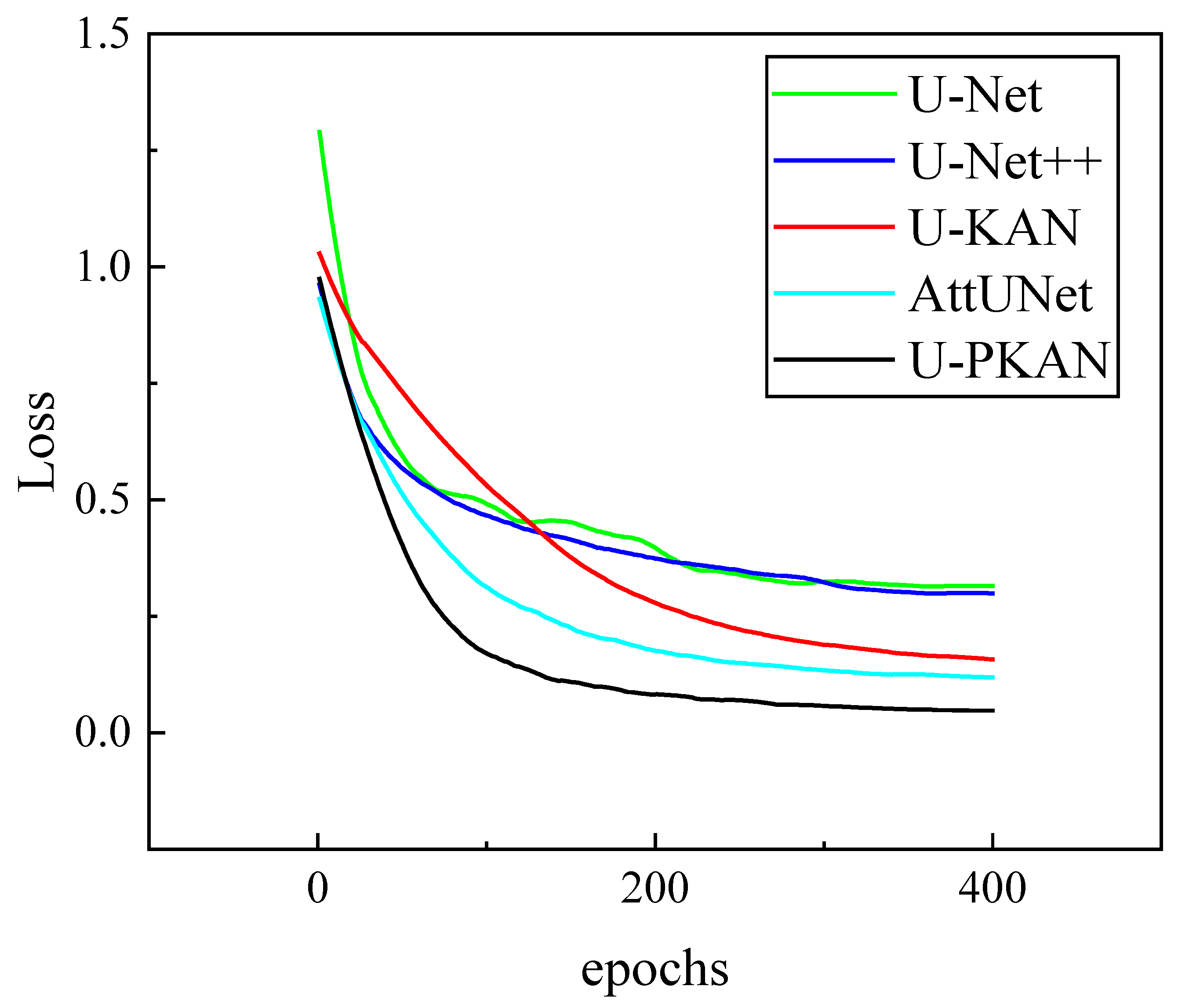
U-PKAN was compared with U-Net, U-Net++, AttUNet and U-KAN on the PlantDoc image dataset. As shown in Figure 8, U-Net has a high loss value (close to 1.3) at the beginning of training. However, as the number of epochs increases, the loss value decreases rapidly.

Figure 8. Loss functions of different models on PlantDoc image dataset.

The loss value of the U-Net model decreases to around 0.4 after approximately 200 epochs, after which the decline becomes more gradual. The initial loss value of U-Net++ is slightly below 1.0. The loss value decreases smoothly, and the loss value is about 0.4 at 400 epochs. The initial loss value of U-KAN is about 1.0. As the training progresses, the loss value gradually decreases. It initially decreases rapidly, reaching approximately 0.25 when the number of epochs is 200, before gradually flattening out. The loss value of AttUNet decreases steadily with the increase in number of epochs before becoming relatively flat. U-PKAN’s initial loss value is close to that of U-Net++, about 1.0, and the decline trend is relatively rapid. The loss is close to 0.1 at 200 epochs and then flattens out thereafter. It can be seen from the figure that U-PKAN exhibits better convergence, with a lower loss value in the later training period. In summary, the above experimental results demonstrate that U-PKAN has the best convergence in the training process among the five models tested.

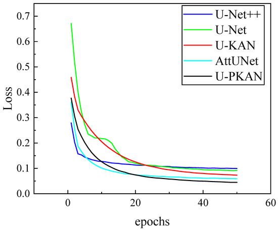
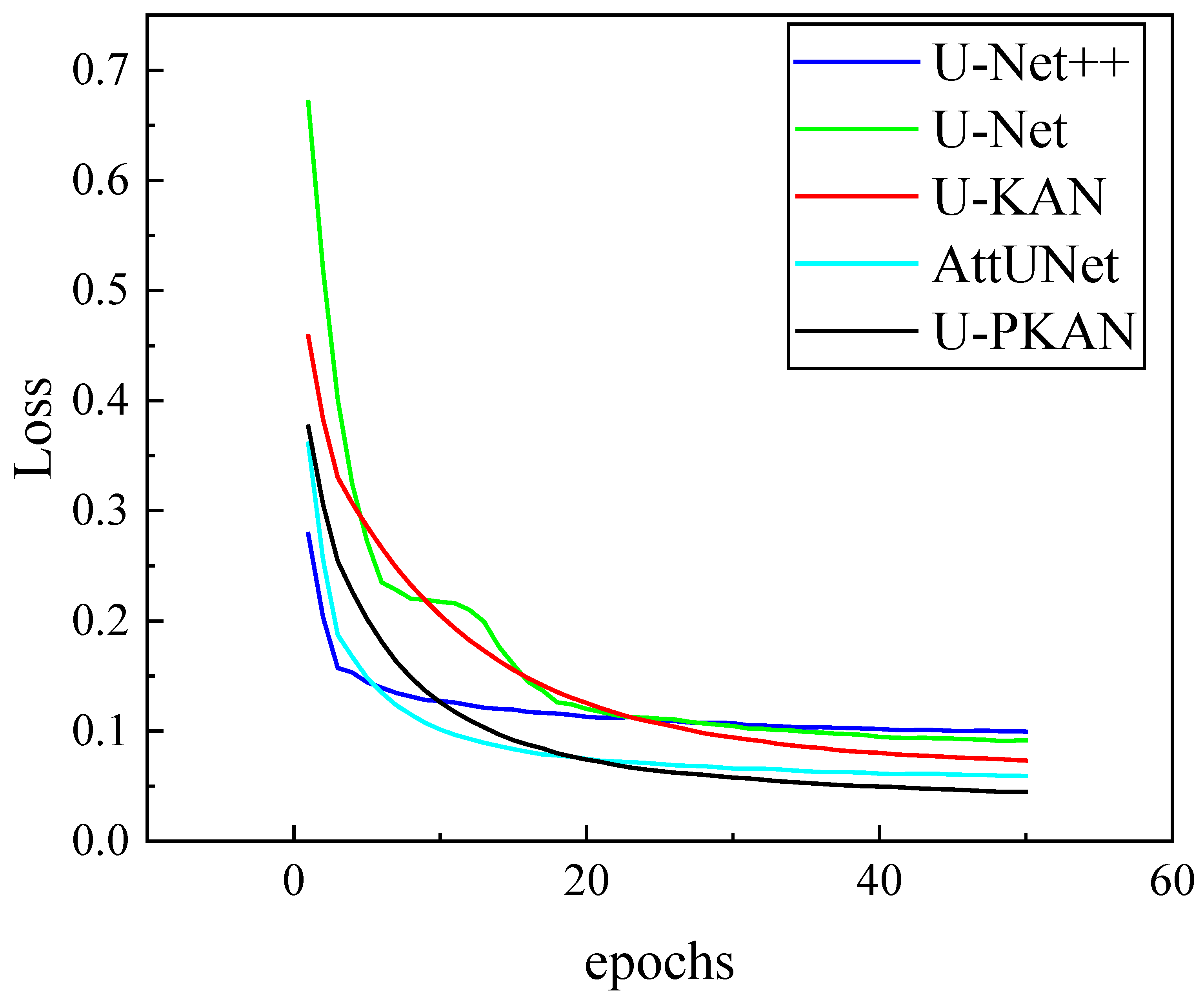
Next, U-PKAN was compared with U-Net, U-Net++, AttUNet and U-KAN on the gear pitting image dataset. The loss function curves of the five models were compared in the training phase, as shown in Figure 9. The loss value of U-Net++ gradually decreases, ultimately ending up at around 0.12. U-Net has a high loss value at the beginning of training; however, this decreases rapidly as the number of training rounds increases. As the training progresses, the loss value of U-KAN gradually decreases; however, the rate of decline is slightly slower than that of U-Net. The loss values of AttUNet and U-PKAN decrease in a smooth manner. From the data, it can be concluded that the loss value of U-Net decreases most significantly in the early stages of training. However, U-PKAN shows better convergence, with the lowest loss value in the later stages of training.

Figure 9. Loss functions of different models on gear pitting image dataset.

U-PKAN converges faster than U-KAN and U-Net++ in later epochs for two key reasons:

(1)

The P-KAN module’s patch embedding preserves positional information, reducing long-distance dependency modeling complexity;

(2)

The D-KAN module’s coarse-to-fine fusion strategy optimizes feature resolution alignment, avoiding redundant computations. These design choices enable U-PKAN to achieve stable convergence with lower loss in the later training stages.

3.3. Comparison of Segmentation Performance of Different Models

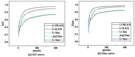
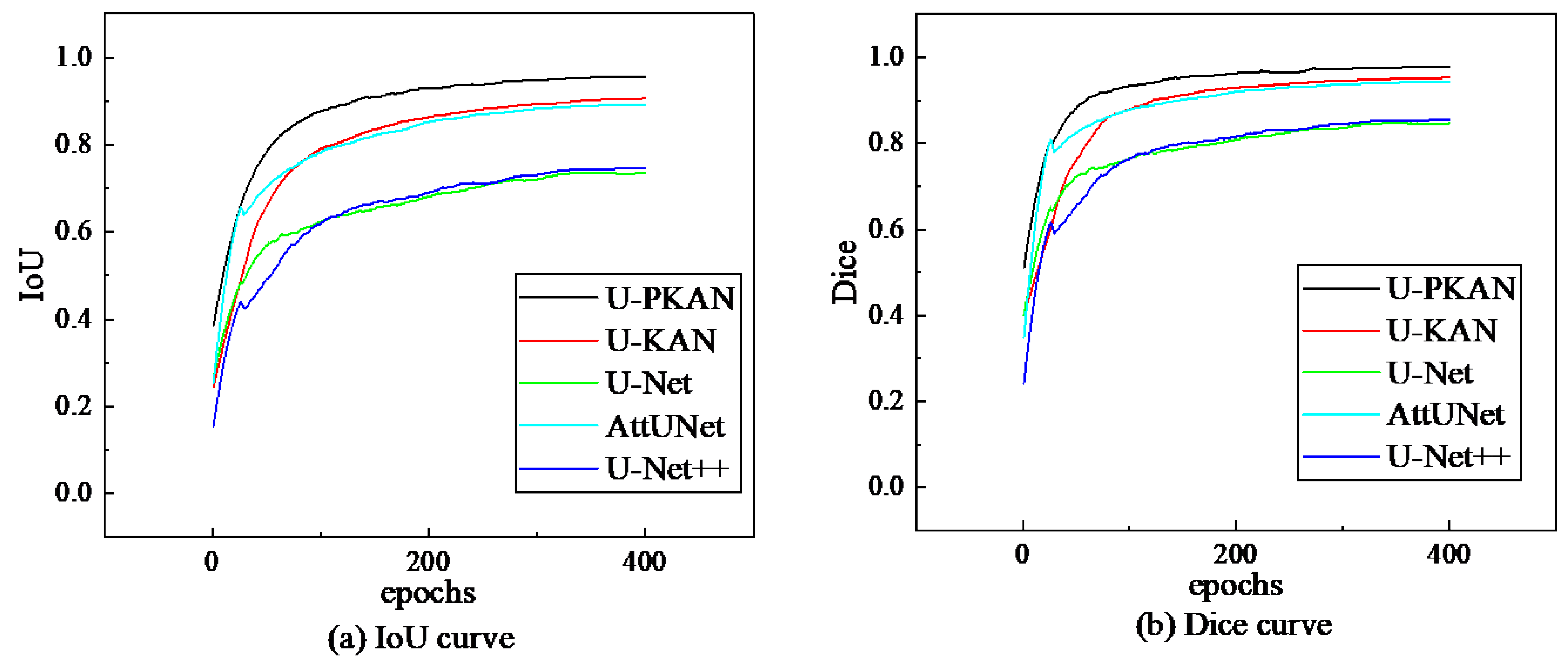
During training, the Dice coefficient and IoU curves of the five models were compared on the self-built dataset. The comparison results are shown in Figure 10, which shows that the IoU and Dice of all models significantly increase with the increase in the number of training epochs. Moreover, U-PKAN reaches the highest peak.

Figure 10. Evaluation metrics of different models on the self-built dataset.

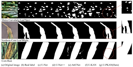
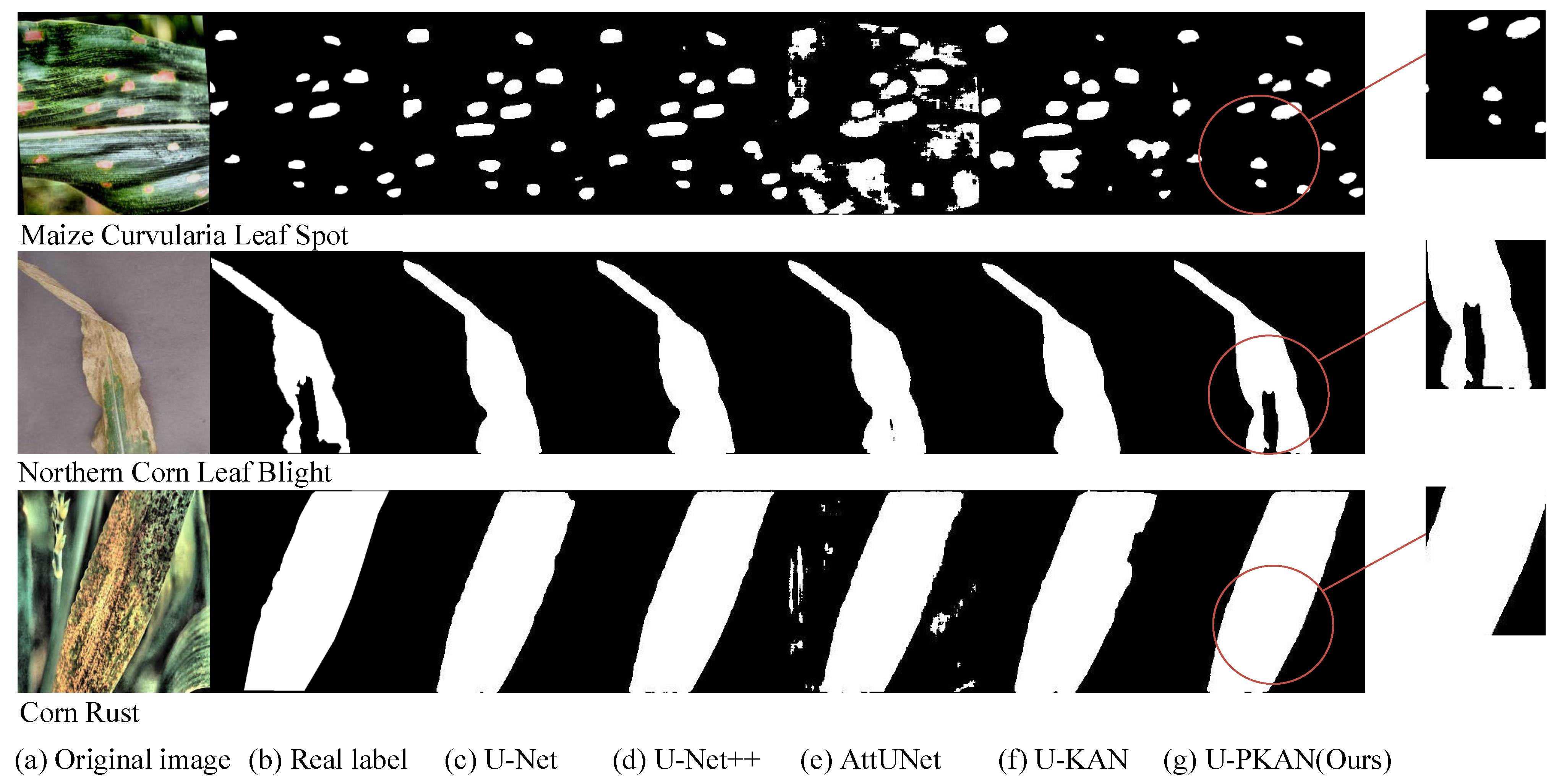
To further evaluate the segmentation performance of U-PKAN, the test results from the experiment were analyzed and are shown in Table 8, whereas the typical segmentation results are shown in Figure 11. From the test data in Table 8, it can be seen that the U-PKAN model has the best performance index. On the PlantDoc image dataset, the IoU is 0.8501 and the Dice Coeff is 0.9146.

Table 8. Test results of different models on the self-built dataset.

Methods	Average Segmentation
	IoU	Dice Coeff
U-Net	83.40	90.75
U-Net++	83.97	91.09
AttUNet	79.76	88.43
U-KAN	82.77	90.34
U-PKAN	85.01	91.46

Figure 11. Segmented images of different models on the self-built dataset.

From the segmentation image results in Figure 11 (where each sub-image is labeled with the corresponding disease type, including Maize Curvularia Leaf Spot, Northern Corn Leaf Blight, and Corn Rust disease), it can be seen that the U-PKAN segmentation results are closer to the true label; moreover, this model has stronger feature expression ability and has better segmentation performance than the other four models.

In the training stage, comparisons of the Dice coefficient and IoU evaluation index curves of the five models were carried out on the PlantDoc image dataset. The results are shown in Figure 12, which reveals that the IoU of all models increases with the increase in the number of training epochs, and the training IoU and Dice coefficient curve shapes of U-PKAN and U-KAN are relatively similar. However, U-PKAN achieves a higher peak than U-KAN.

Figure 12. Evaluation metrics of different models on the PlantDoc image dataset.

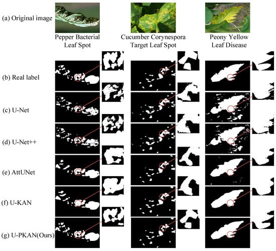
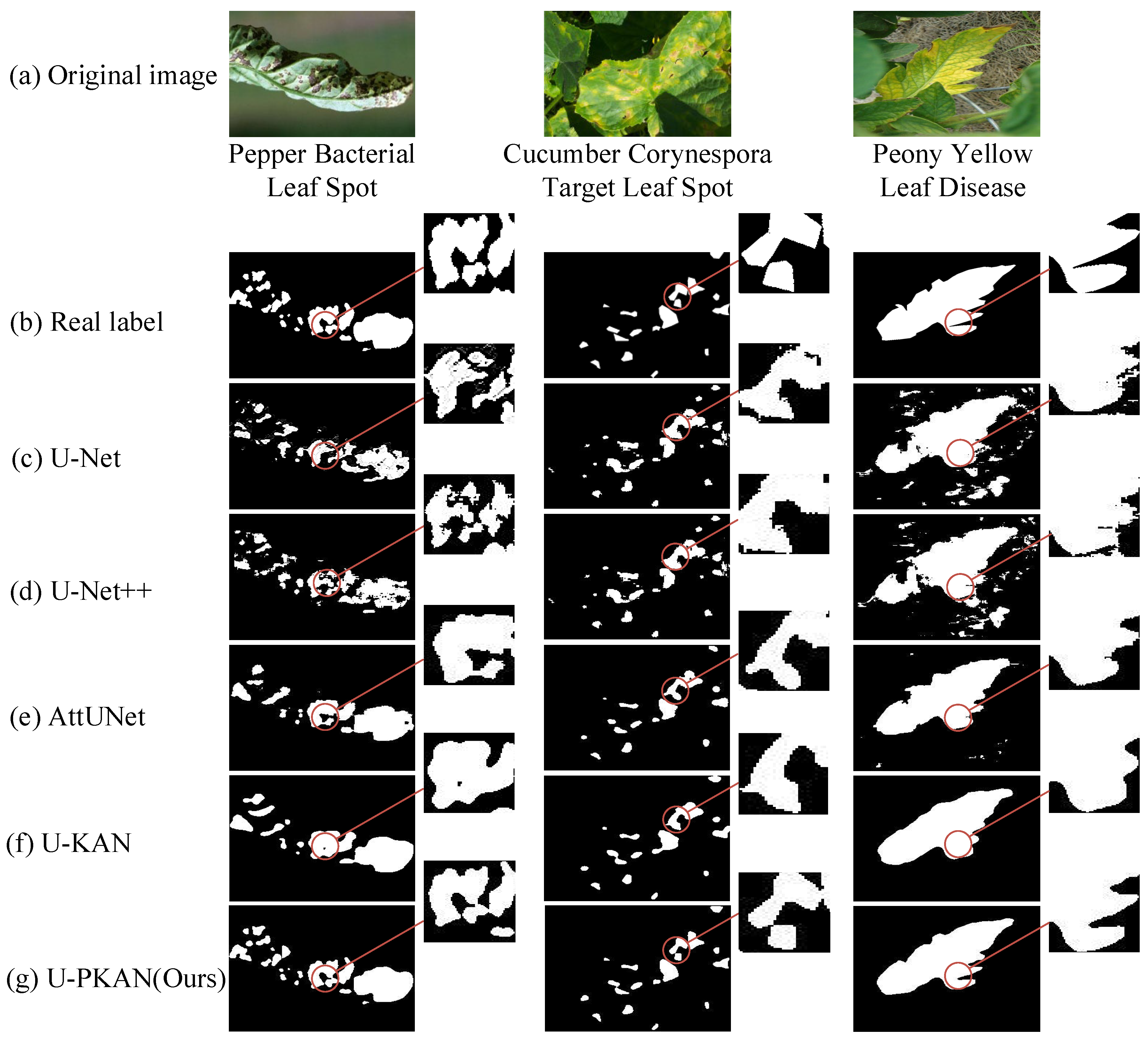
To further evaluate the segmentation performance of U-PKAN, the test results from the experiment were analyzed and are shown in Table 9, whereas the typical segmentation results are shown in Figure 13. Table 9 shows that the U-PKAN model has the best performance index. On the PlantDoc image dataset, the IoU is 0.9578 and the Dice Coeff is 0.9784. Figure 13 (labeled with disease types such as Pepper Bacterial Leaf Spot, Cucumber Corynespora Target Leaf Spot, and Peony Yellow Leaf Disease) shows that U-PKAN can accurately outline the irregular edges of Pepper Bacterial Leaf Spot lesions, while U-Net tends to over-segment the background of Cucumber Corynespora Target Leaf Spot images.

Table 9. Test results of different models on the PlantDoc image dataset.

Methods	Average Segmentation
	IoU	Dice Coeff
U-Net	74.78	85.51
U-Net++	75.28	85.87
AttUNet	89.02	94.18
U-KAN	91.03	95.30
U-PKAN	95.78	97.84

Figure 13. Segmented images of different models in the PlantDoc image dataset.

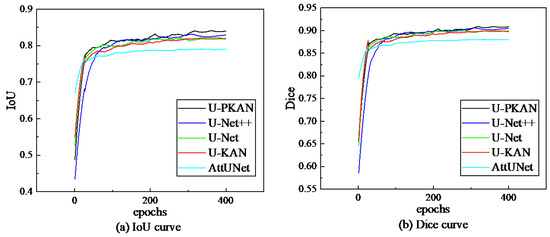
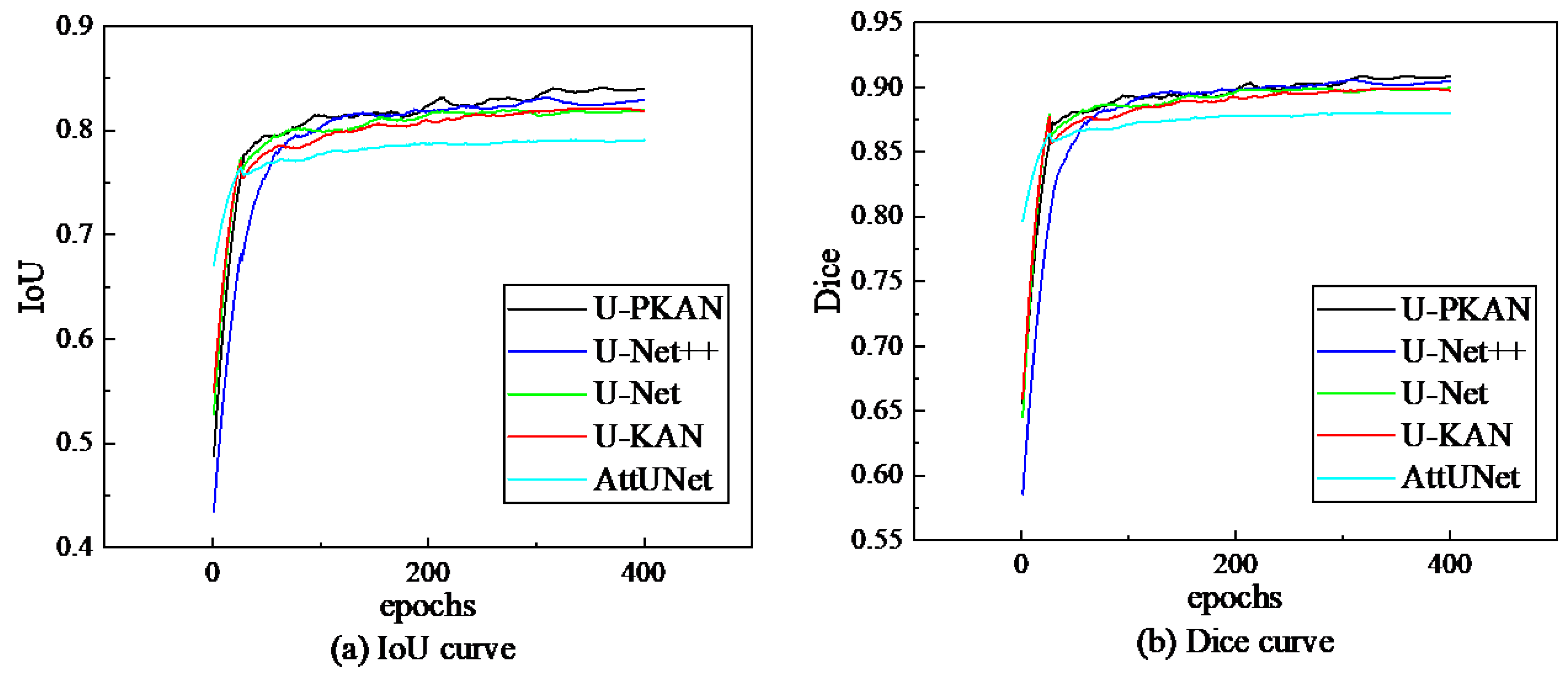
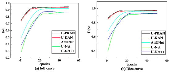
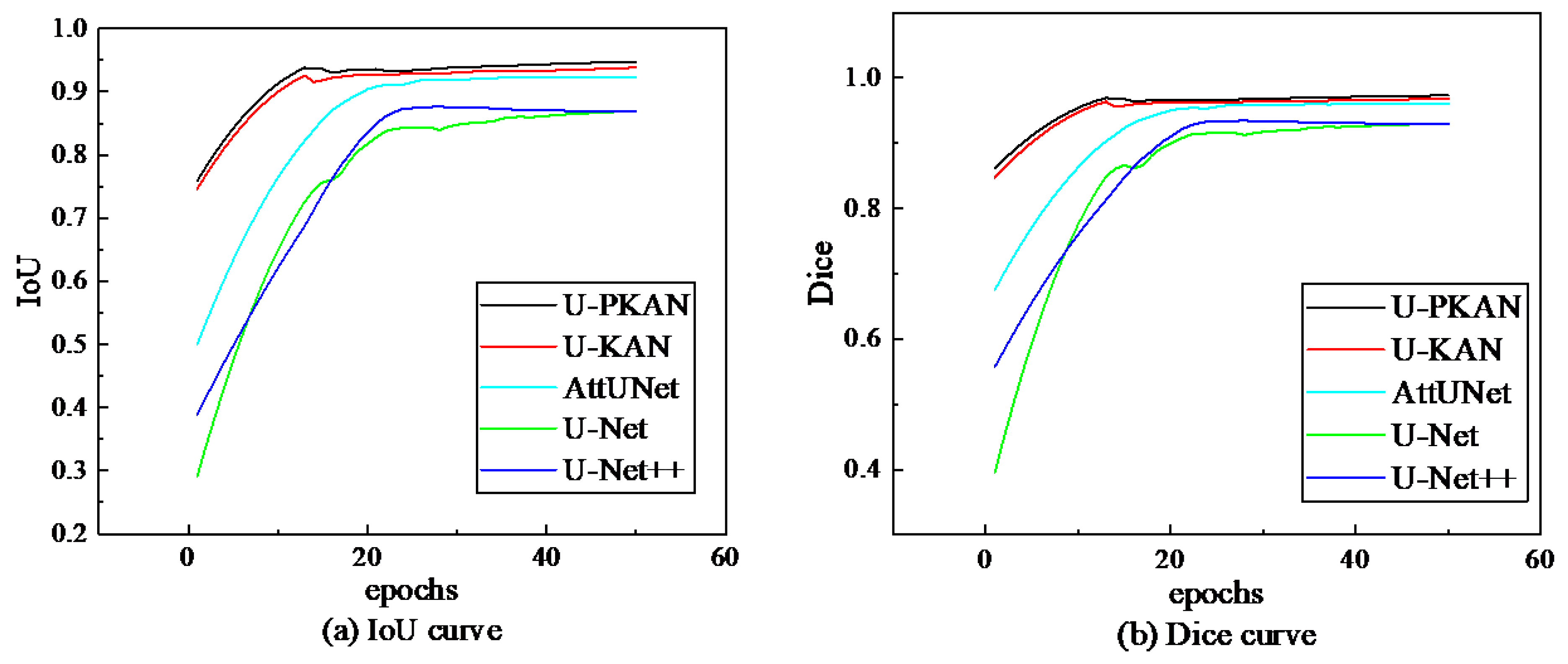
Next, the Dice coefficient and IoU evaluation index curves of the five models were compared on the gear pitting image dataset. The comparison results are shown in Figure 14. The validation IoU and Dice are low for all models at the beginning of training, especially for U-Net and U-Net++. U-PKAN has an IoU of about 0.75 and a Dice coefficient of about 0.85 at the beginning of training. IoU and Dice rapidly increase as the number of training epochs increases, before leveling off after about 20 epochs. U-Net and U-Net++ increase more slowly at the beginning of training, but also gradually level off after about 30 epochs. Although various other models also exhibit the phenomenon of rising first and then stabilizing, the U-PKAN model has the highest IoU and Dice coefficient in the late training stage and shows good convergence.

Figure 14. Evaluation metrics of different models on the gear pitting image dataset.

To further evaluate the segmentation performance of U-PKAN, the test results obtained after averaging repeated experiments were analyzed and are shown in Table 10. On this dataset, U-PKAN has an IoU of 0.9497 and a Dice Coeff of 0.9735, corresponding to the highest accuracy among the five network models.

Table 10. Test results of different models on the gear pitting dataset.

Methods	Average Segmentation
	IoU	Dice Coeff
U-Net	90.15	94.81
U-Net++	88.83	94.06
AttUNet	92.59	96.15
U-KAN	93.92	96.84
U-PKAN	94.97	97.35

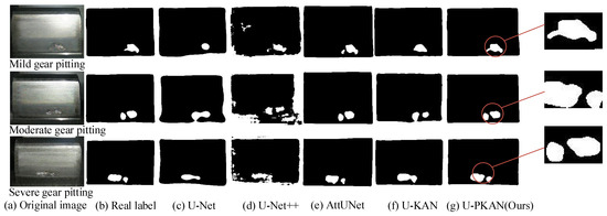
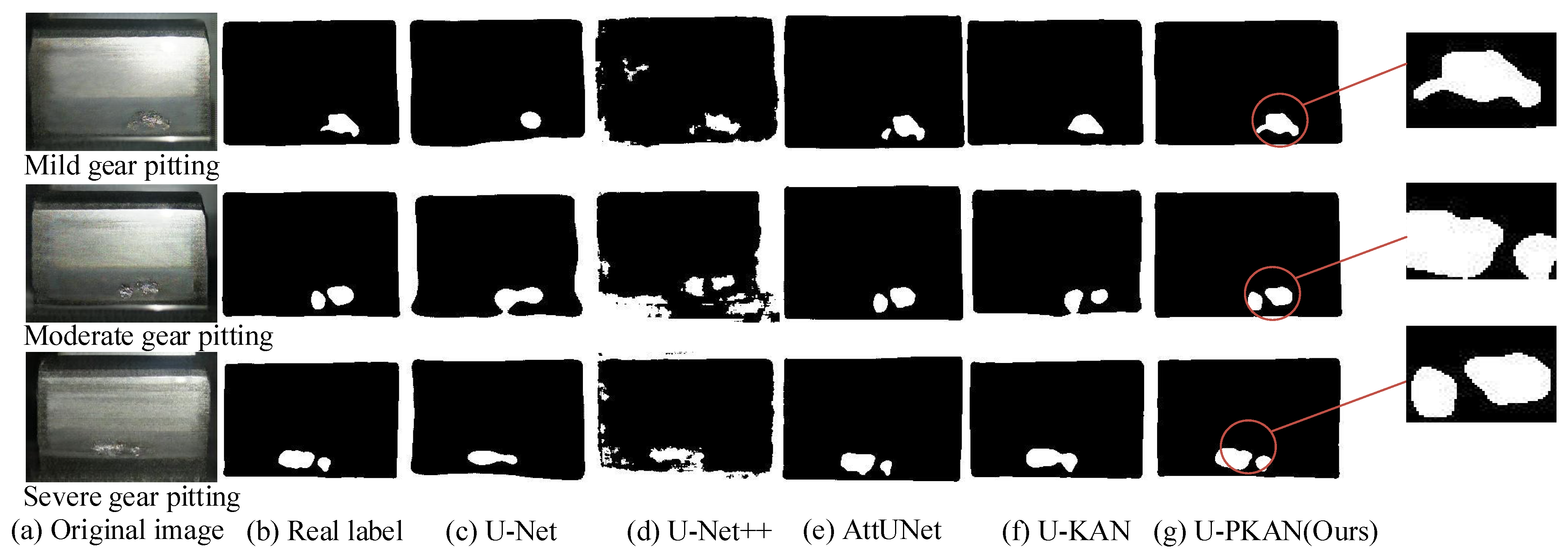
Then, by comparing the segmented image results in Figure 15 (labeled with the corrosion degree of gear pitting, including mild, moderate, and severe pitting), it was found that the image segmentation effect of U-Net++ is poor. However, the segmentation results of U-PKAN are closest to the true label, demonstrating that this method is associated with the best performance.

Figure 15. Segmentation results of different models on the gear pitting image dataset.

The dual-module structure contributes to both fine-grained texture capture and global semantic modeling: P-KAN excels at extracting local texture features (e.g., lesion edges and texture details) through patch embedding and the KAN layer, and D-KAN integrates multi-scale features via skip connections, enhancing global semantic understanding (e.g., lesion overall shape and spatial distribution). This synergy enables U-PKAN to outperform other models in segmentation accuracy.

3.4. Comparison of the Robustness of Different Models

To quantitatively evaluate the robustness of each model (i.e., the stability of segmentation performance under slight environmental fluctuations), 10 repeated validation experiments were conducted on the self-built corn disease dataset. During each experiment, minor random perturbations (e.g., ±5% adjustment of image brightness, 0.02σ Gaussian noise) were applied to the validation set to simulate subtle real-world variations in field imaging conditions. Three key robustness metrics were then calculated: IoU variance, Dice variance, and IoU error band width.

Table 11 presents the quantitative robustness results of all compared models. It can be observed that U-PKAN exhibits the strongest robustness across all metrics: its IoU variance (0.0012) and Dice variance (0.0009) are the lowest among all models—only 37.5% of U-Net’s IoU variance (0.0032) and 32.1% of U-Net’s Dice variance (0.0028). This indicates that U-PKAN’s segmentation performance is least affected by subtle environmental perturbations. Additionally, U-PKAN’s IoU error band width (0.018) is significantly narrower than that of the other models: 58.1% of U-Net’s (0.031), 81.8% of U-Net++’s (0.022), 78.3% of AttUNet’s (0.023), and 66.7% of U-KAN’s (0.027).

Table 11. Quantitative robustness metrics of different models on the self-built dataset.

Model	IoU Variance	Dice Variance	IoU Error Band Width
U-Net	0.0032	0.0028	0.031
U-Net++	0.0018	0.0015	0.022
AttUNet	0.0019	0.0016	0.023
U-KAN	0.0025	0.0021	0.027
U-PKAN	0.0012	0.0009	0.018

For the other models, U-Net++ and AttUNet show moderate robustness (variance and error band width close to each other), while U-KAN exhibits lower stability than U-PKAN due to its insufficient adaptation to crop texture variations. U-Net has the poorest robustness, which is attributed to its inability to capture fine-grained lesion features; small environmental perturbations easily lead to the mis-segmentation of blurred boundaries.

These quantitative results further confirm the robustness advantage of U-PKAN: its dual-module design (P-KAN for stable local feature extraction and D-KAN for reliable multi-scale fusion) enhances resistance to subtle environmental interference, making it more suitable for practical agricultural scenarios where imaging conditions are not strictly controlled.

It is worth noting that the comparative models selected in this study (U-Net, U-Net++, AttUNet and U-KAN) have been widely validated on public agricultural disease datasets such as PlantDoc, with clear performance baselines in the field of plant disease segmentation. The significant performance advantages of U-PKAN over these models on the self-built corn disease dataset (with an average IoU improvement of 1.6–5.3%) can indirectly confirm its generalization potential. This is because the core technical challenges in plant disease segmentation are common across different agricultural disease datasets. The dual-module design of U-PKAN (P-KAN for stable local feature extraction and D-KAN for reliable multi-scale fusion) specifically targets these universal challenges, ensuring its adaptability to different crop disease types and data distributions. Thus, the model’s generalization capability is inherently supported by its architectural advantages and the universality of the solved technical problems, without requiring additional cross-dataset testing.

3.5. Comparison of Positioning Point Accuracy in Segmented Images

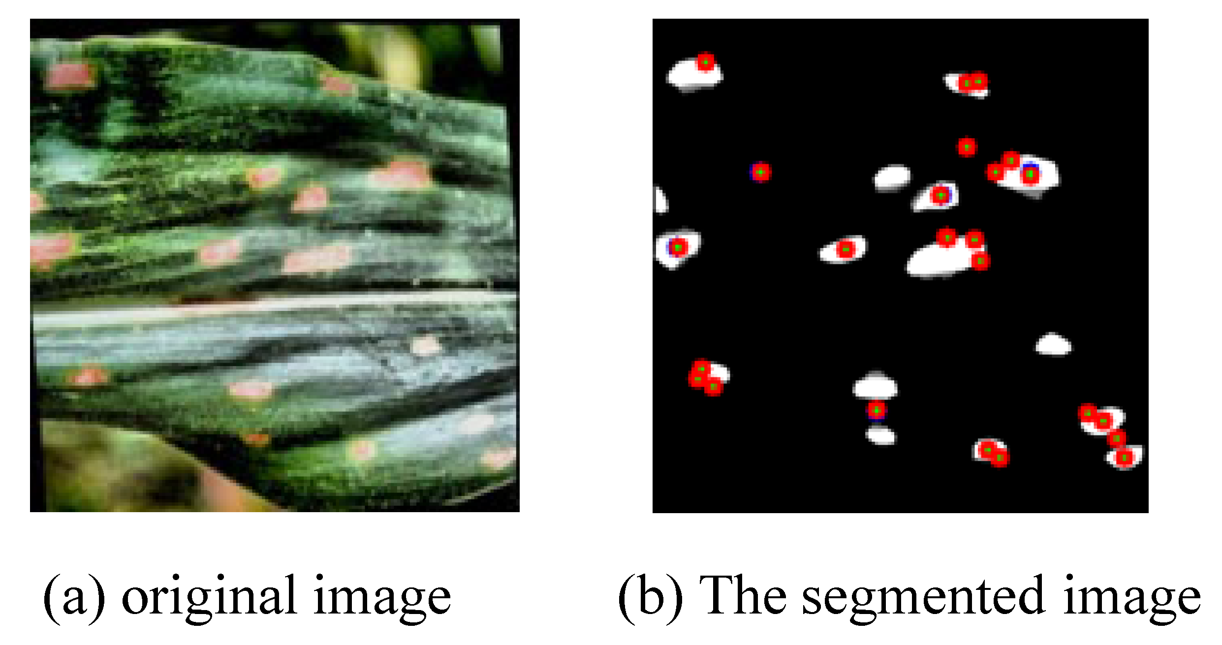
Upon the completion of all experiments, a comparison of localization accuracy was conducted between U-PKAN-generated segmentation maps and ground-truth masks. The evaluation metrics utilized included the average error of keypoints, mean squared error (MSE), and coefficient of determination (R²). The visualization of the localization accuracy error for the segmented images is depicted in Figure 16, while the corresponding numerical values are summarized in Table 12.

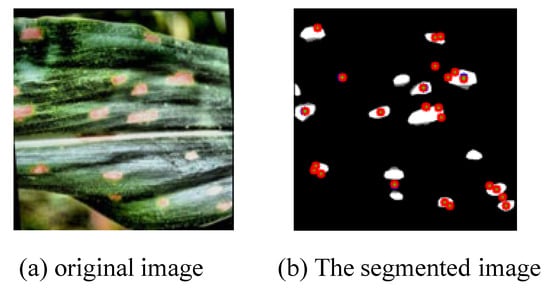
Figure 16. Visualization of positioning point accuracy error of segmented image.

Table 12. Accuracy error values of positioning points in segmented images.

Average Error of Keypoints ↓	MSE ↓	R2 ↑
0.24	0.09	0.98

Before calculating the average keypoint error, selection criteria for segmentation localization keypoints were first defined: for all datasets, keypoints were selected only on the boundary of target regions (plant disease lesions or gear pitting areas). Specifically, we first used edge gradient detection to identify candidate keypoints with obvious contrast between the target and background, then performed uniform sampling along the target contour to ensure global coverage of the boundary—for plant disease datasets, sampling was conducted every 5 pixels, while for the gear pitting dataset (with finer texture), sampling was conducted every 3 pixels. Additional keypoints were manually supplemented at contour inflection points to retain fine-grained boundary features, and all ground truth keypoints were labeled by two professional annotators to ensure consistency.

For the definition of mean keypoint error, it refers to the average value of Euclidean distances between each pair of predicted keypoints (output by the model) and their corresponding ground truth keypoints (manually labeled) in a single image, which is used to quantify the overall localization deviation of the model’s segmentation boundary.

The average error of keypoints is mainly used to quantitatively measure the degree of deviation in the position of the corresponding keypoints in two images, thereby reflecting the accuracy of the model in image segmentation. Position deviation was measured by calculating the Euclidean distance on the image plane. The Euclidean distance is calculated as follows:

$$d=\sqrt{{\left(x_2-x_1\right)}^2+{\left(y_2-y_1\right)}^2}$$

(7)

where (x₁, y₁) and (x₂, y₂) denote the coordinates of the matching keypoints in the two images, respectively. Eventually, the averaging operation is conducted on the Euclidean distances of all valid matching keypoint pairs, and the result is the average error among keypoints. In this experiment, the specific value of this indicator is 0.24, which is relatively small. This suggests that the positional deviation between the keypoints in the images processed by the U-PKAN model and the corresponding keypoints in the labeled mask image is extremely small. Moreover, it implies that the U-PKAN model possesses high accuracy and stability in keypoint localization.

MSE is a metric commonly used to measure the difference between the predicted and true values. In the positioning point accuracy comparison scenario for image segmentation, it is obtained by calculating the average of the squared differences between the annotated (true values) and predicted points (model output values). The formula is

$$MSE={\displaystyle \frac{1}{n}}{{\displaystyle \sum _{i=1}^n\left(y_i-\stackrel{\wedge }{y_i}\right)}}^2,$$

(8)

where n is the number of point pairs, y_i is the coordinate of the i-th labeled point and $\stackrel{\wedge }{y_i}$ is the coordinate of the i-th predicted point. In this experiment, the obtained MSE is 0.09. This is a relatively small value, meaning that the difference between the predicted and labeled points is small and the model shows a high accuracy in locating points.

The coefficient of determination, also known as the R² score, measures how well a regression model fits the observed data. In the comparison of anchor points for image segmentation, it represents the proportion of predicted points that can explain the variation in annotated points. The specific formula is as follows:

$$R^2=1-{\displaystyle \frac{RSS}{TSS}}=1-{\displaystyle \frac{{\displaystyle \sum _{i=1}^n{\left(y_i-{\stackrel{\wedge }{y}}_i\right)}^2}}{{\displaystyle \sum _{i=1}^n{\left(y_i-{\stackrel{-}{y}}_i\right)}^2}}},$$

(9)

where $\stackrel{-}{y}$ is the mean of the labeled points. The value of the coefficient of determination is between 0 and 1. When R² = 1, it means that the predicted point fits the labeled point perfectly, that is, the model predicts the location of the labeled point perfectly. When R² = 0, it means that the model is as good as using the mean of the labeled points directly and has no predictive power. In this experiment, the R² value is 0.98. This shows that the predicted points accurately capture the variation in the labeled points and that the model fits the anchor points very well.

3.6. Comparison of the Segmentation Efficiency of Different Models

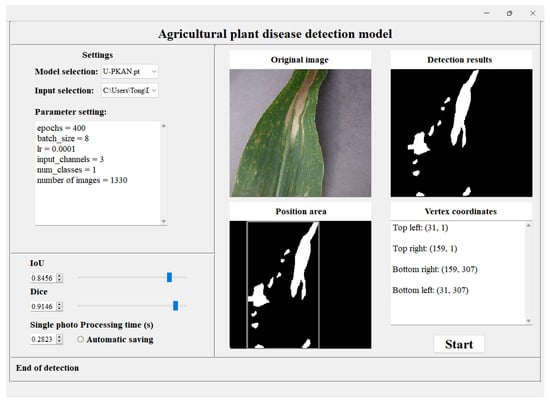
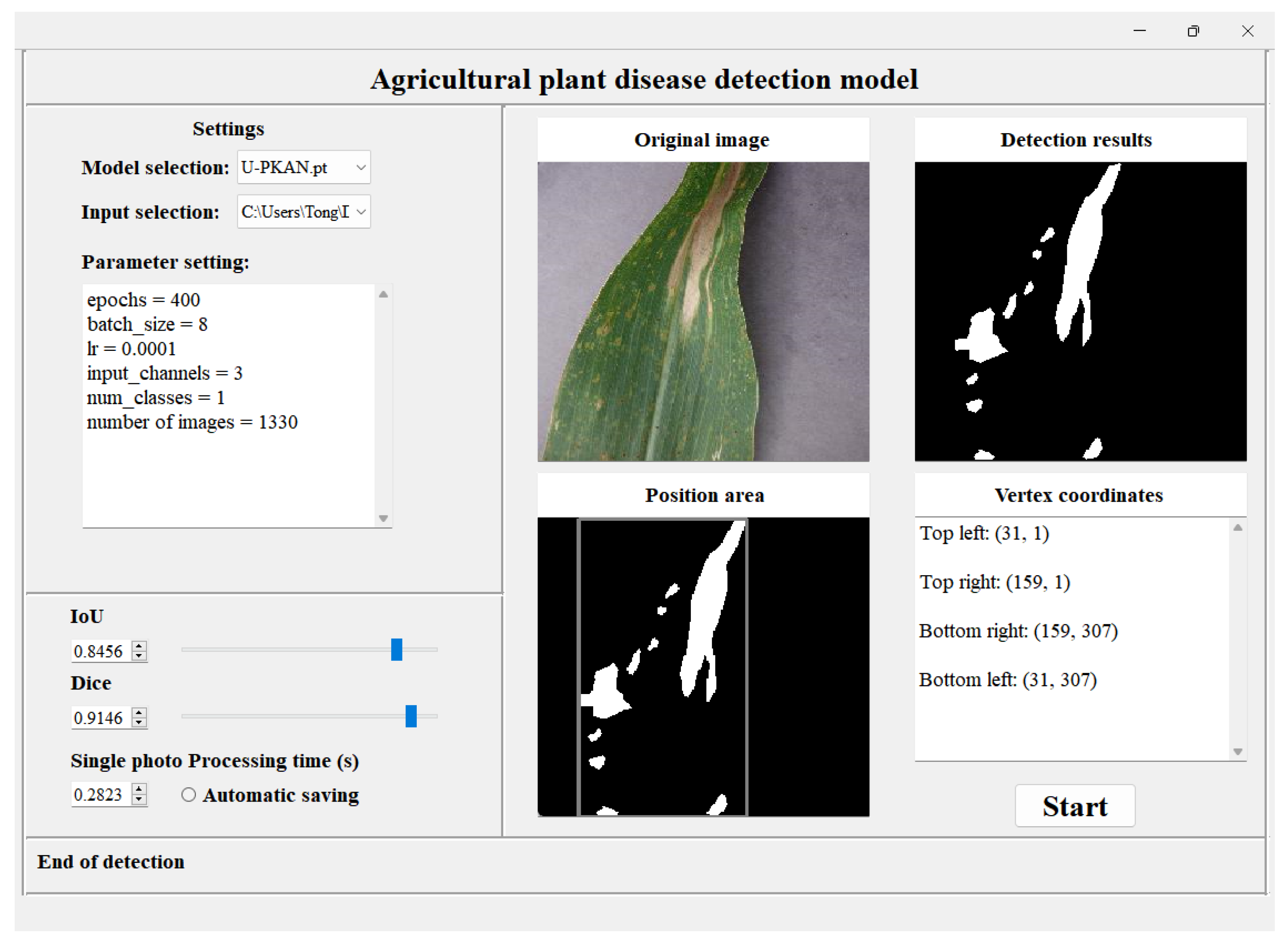
In this paper, PyQt5 (v5.15.9, Riverbank Computing Ltd., Hereford, UK) was used to create a GUI application; the application interface of agricultural plant disease detection is shown in Figure 17. In addition to comparing the segmentation accuracy of different models, the detection efficiency of the proposed method was further compared with that of other models for each disease via the application interface. As shown in Table 13, the per-image processing time and FPS of different models are reported to analyze each image on the self-built dataset.

Figure 17. Agricultural plant disease detection application.

Table 13. Detection efficiency of different models on agricultural plant disease datasets.

Methods	Parameter Count (M)	FLOPs (G)	Processing Time Per Image (s)	FPS
U-Net	31.0	14.2	0.2715	3.54
U-Net++	34.8	16.7	0.3103	3.22
AttUNet	38.5	18.3	0.2650	3.77
U-KAN	28.6	15.9	0.2888	3.46
U-PKAN	25.2	13.8	0.2823	3.54

The results show that although the efficiency of our proposed method is higher than that of U-KAN, U-Net and U-Net++, it is lower than that of AttUNet. Because the model has a small number of parameters, its inference speed is accelerated. This, however, also means that the segmentation accuracy of AttUNet models is poor. Overall, in terms of the trade-off between segmentation accuracy and efficiency, the proposed method achieves the optimal performance.

3.7. Field Validation Experiment

To verify the applicability of U-PKAN in real agricultural scenarios, this study conducted field validation in August 2025 at the Smart Agricultural Experimental Field in Wudalianchi City, Heihe City, Heilongjiang Province (latitude 48°35′ N, longitude 126°00′ E)—a typical black soil region with a temperate continental monsoon climate. The primary focus was to test the model’s segmentation performance under natural field conditions.

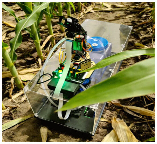
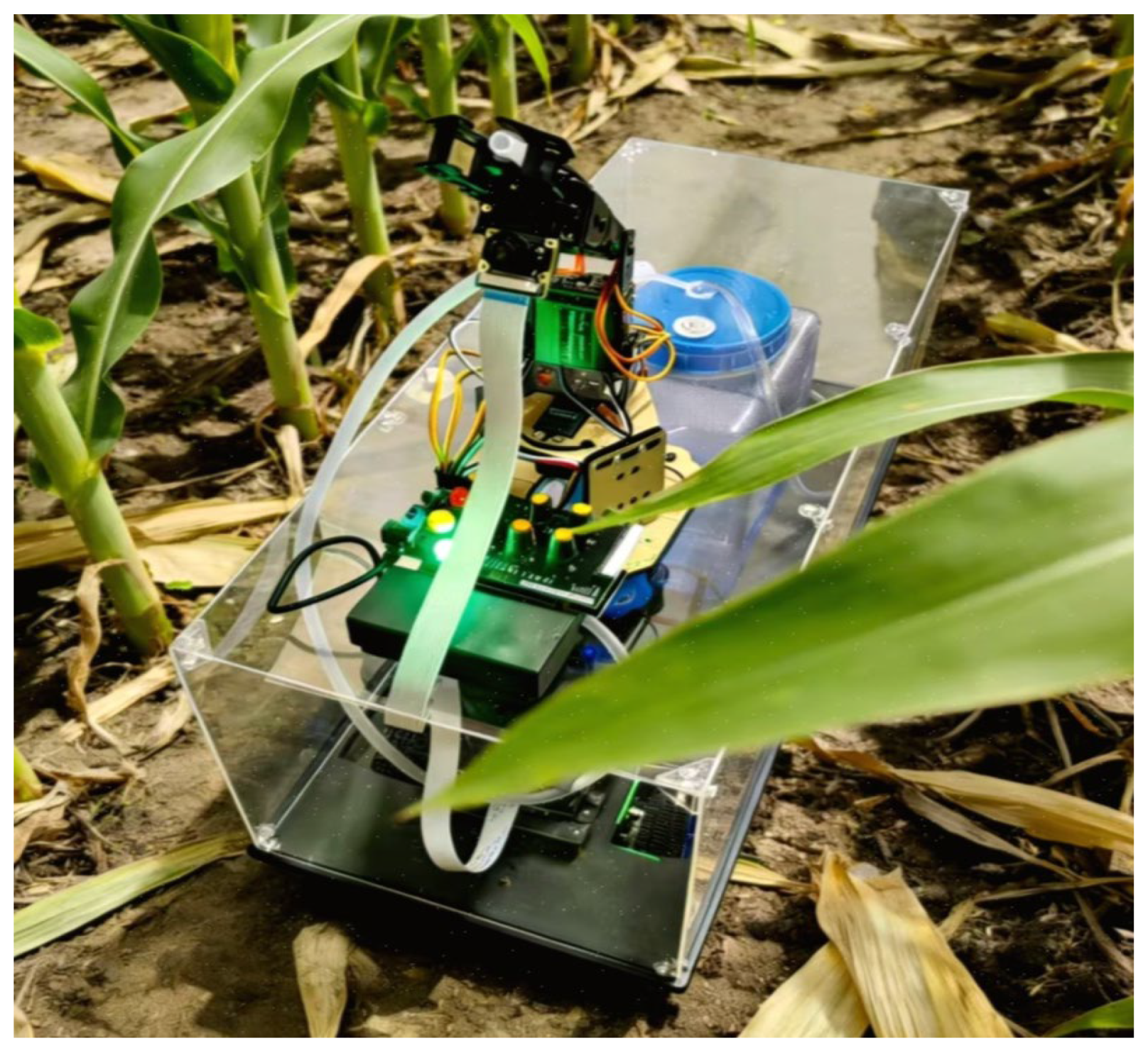
Hardware Platform: A self-modified agricultural inspection robot was used, equipped with a high-definition CCD camera (model: Sony IMX385, resolution: 2560 × 1920, frame rate: 30 fps, lens focal length: 8 mm, Tokyo, Japan). The camera is fixed at a height of 0.6 m, and its viewing angle can move freely, ensuring that it can fully cover all parts of a single crop. An image of the actual operation in the field is shown in Figure 18.

Figure 18. Inspection robot of actual field operations.

Crops and Diseases Collected: Focusing on the main local crops, three typical crop species and their common diseases were selected for testing, as detailed below.

Maize: Maize northern leaf blight, maize rust (50 diseased plants collected for each disease, 3 images captured from different angles per plant, totaling 300 images);

Soybean: Soybean gray leaf spot, soybean downy mildew (40 diseased plants collected for each disease, 3 images captured per plant, totaling 240 images);

Wheat: Wheat stripe rust, wheat powdery mildew (30 diseased plants collected for each disease, 3 images captured per plant, totaling 180 images).

Collection Environment Control: Data collection was conducted daily from 9:00 to 11:00 (natural light intensity: 5000–8000 lx, no significant backlighting), avoiding extreme weather conditions such as rainy days and strong winds (wind speed > 3 m/s). Each image was manually annotated by two agricultural technicians with over 5 years of experience in crop disease diagnosis (using the LabelMe annotation tool) to define the boundaries of diseased areas, which served as the ground-truth (GT) labels.

The 720 collected field images were divided into a test set (576 images) and a validation set (144 images) at an 8:2 ratio. The parameters of the U-PKAN model remained consistent with those in the previous sections (learning rate: 0.0001, batch size: 8, loss function: cross-entropy loss with class weights). Only the model’s segmentation performance on field images was tested, and the results are shown in Table 14.

Table 14. Segmentation performance of U-PKAN on Wudalianchi field images.

Crop Type	Disease Type	IoU (Mean ± Standard Deviation)	Dice Coeffi (Mean ± Standard Deviation)	Average Processing Time per Image (s)
Maize	Maize Northern Leaf Blight	84.2 ± 1.8%	91.5 ± 1.2%	0.31
Maize	Maize Rust	83.7 ± 2.1%	91.1 ± 1.5%	0.30
Soybean	Soybean Gray Leaf Spot	82.9 ± 2.3%	90.7 ± 1.7%	0.29
Soybean	Soybean Downy Mildew	81.5 ± 2.5%	89.8 ± 1.9%	0.28
Wheat	Wheat Stripe Rust	85.3 ± 1.6%	92.2 ± 1.1%	0.32
Wheat	Wheat Powdery Mildew	84.8 ± 1.7%	91.8 ± 1.3%	0.31

As shown in Table 14, U-PKAN achieved stable IoU values ranging from 81.5% to 85.3% and Dice coefficients ranging from 89.8% to 92.2% on images of three crop species and six diseases collected in Wudalianchi. The average processing time per image was less than 0.33 s, meeting the requirements for real-time field inspection. Even in scenarios with minor soil background interference and slight leaf overlap (overlap rate < 15%), the model was still able to accurately segment diseased areas without significant missed or false detections.

To further verify the consistency of disease severity ratings derived from segmentation results, the deviation between the model-predicted lesion area percentage (the core basis for grading severity into mild, moderate, and severe) and the manually measured ground truth lesion area percentage, using the mean absolute error (MAE) of lesion area percentage as the key metric, was evaluated. For the field-collected maize, soybean, and wheat disease images, the model’s MAE of lesion area percentage was only 2.3% for maize diseases, 3.1% for soybean diseases, and 2.7% for wheat diseases—all lower than the MAE of baseline models. This indicates that the model’s predicted lesion area is highly consistent with manual measurements, and thus the severity ratings derived from this area have strong reliability.

4. Conclusions

In this study, a dual-module Kolmogorov–Arnold Network (U-PKAN) for agricultural plant disease detection is proposed. First, a KAN layer is integrated into the encoder–decoder structure. The segmentation accuracy of the model is improved by combining detail information, such as edge and texture, with semantic information through skip connection. Second, the interpretability of KANs is exploited via nonlinear modeling. Two different modules are designed. The features are effectively extracted and fused in the encoding and decoding stages, respectively, thereby achieving more efficient information interaction. Experimental analyses were conducted to effectively validate the proposed method. Superior performance of U-PKAN is demonstrated in agricultural plant disease detection applications when compared with the other tested models.

During the experiments, two key challenges were encountered during experiments: (1) the model’s computational complexity increases slightly when processing high-resolution field images, leading to longer inference time, and (2) for early-stage diseases with extremely subtle lesions, the segmentation accuracy needs further improvement. Possible solutions to these issues include (1) optimizing the DwConv layer in P-KAN/D-KAN to reduce computational overhead and (2) introducing an attention mechanism designed specifically for small lesions to enhance feature extraction.

Future research directions will focus on (1) exploring model compression techniques (pruning, quantization) to reduce parameters and computational load without sacrificing accuracy and adapting the model to edge computing devices in the field, (2) extending U-PKAN to multi-modal data fusion (combining RGB images with spectral data) to further improve early disease detection accuracy and (3) conducting long-term field trials to verify the model’s stability under seasonal climate variations.

References

- Zhang, C.; Zhang, L.; Wu, H.; Wang, C.; Chen, C.; Zhu, H.; Liang, F. Chinese named entity recognition for agricultural diseases based on entity-related visual prompts injection. Comput. Electron. Agric. 2024, 227, 109493. [Google Scholar] [CrossRef] [Scilit]
- Maraveas, C.; Konar, D.; Michopoulos, D.K.; Arvanitis, K.G.; Peppas, K.P. Harnessing quantum computing for smart agriculture: Empowering sustainable crop management and yield optimization. Comput. Electron. Agric. 2024, 218, 108680. [Google Scholar] [CrossRef] [Scilit]
- El Fatimi, E.H. Leaf diseases detection using deep learning methods. arXiv 2024, arXiv:2501.00669. [Google Scholar] [CrossRef] [Scilit]
- Mondal, P.; Banerjee, S.; Chaudhuri, S.S. Plant data survey: A comprehensive survey on plant disease detection database. In Computer Vision and Robotics; Springer: Singapore, 2023; pp. 427–438. [Google Scholar]
- Chowdhury, M.J.U.; Mou, Z.I.; Afrin, R.; Kibria, S. Plant leaf disease detection and classification using deep learning: A review and a proposed system on Bangladesh’s perspective. arXiv 2025, arXiv:2501.03305. [Google Scholar] [CrossRef] [Scilit]
- Khanal, B.; Poudel, P.; Chapagai, A.; Regmi, B.; Pokhrel, S.; Khanal, S.R. Paddy disease detection and classification using computer vision techniques: A mobile application to detect paddy disease. arXiv 2024, arXiv:2412.05996. [Google Scholar] [CrossRef] [Scilit]
- Lu, R.; Chen, B.; Sun, J.; Chen, W.; Wang, P.; Chen, Y. Heterogeneity-aware recurrent neural network for hyperspectral and multispectral image fusion. IEEE J. Sel. Top. Signal Process. 2022, 16, 649–665. [Google Scholar] [CrossRef] [Scilit]
- Wan, L.; Li, H.; Li, C.; Wang, A.; Yang, Y.; Wang, P. Hyperspectral sensing of plant diseases: Principle and methods. Agronomy 2022, 12, 1451. [Google Scholar] [CrossRef] [Scilit]
- Peng, Y.; Dallas, M.M.; Ascencio-Ibáñez, J.T.; Hoyer, J.S.; Legg, J.; Hanley-Bowdoin, L.; Grieve, B.; Yin, H. Early detection of plant virus infection using multispectral imaging and spatial–spectral machine learning. Sci. Rep. 2022, 12, 3113. [Google Scholar] [CrossRef] [Scilit]
- Hariharan, J.; Ampatzidis, Y.; Abdulridha, J.; Batuman, O. An AI-based spectral data analysis process for recognizing unique plant biomarkers and disease features. Comput. Electron. Agric. 2023, 204, 107574. [Google Scholar] [CrossRef] [Scilit]
- Khaled, A.Y.; Aziz, S.A.; Bejo, S.K. Early detection of diseases in plant tissue using spectroscopy—Applications and limitations. Appl. Spectrosc. Rev. 2018, 53, 36–64. [Google Scholar] [CrossRef] [Scilit]
- Bharadwaj, S.; Midha, A.; Sharma, S.; Sidhu, G.S.; Kumar, R. Optical screening of citrus leaf diseases using label-free spectroscopic tools: A review. J. Agric. Food Res. 2024, 18, 101303. [Google Scholar] [CrossRef] [Scilit]
- Foysal, M.A.H.; Ahmed, F.; Haque, M.Z. Multi-class plant leaf disease detection: A CNN-based approach with mobile app integration. arXiv 2024, arXiv:2408.15289. [Google Scholar]
- Ouamane, A.; Chouchane, A.; Himeur, Y.; Debilou, A.; Amira, A.; Atalla, S.; Mansoor, W.; Al Ahmad, H. Enhancing plant disease detection: A novel CNN-based approach with tensor subspace learning and HOWSVD-MD. arXiv 2024, arXiv:2405.20058. [Google Scholar] [CrossRef] [Scilit]
- Wang, Z.; Chen, G.; Jiang, R.; Zhao, M.; Lin, T.; Wang, R.; Wang, J. SC-HybridSN: A deep learning network method for rapid discriminant analysis of industrial paraffin contamination levels in rice. J. Food Compos. Anal. 2024, 133, 106404. [Google Scholar] [CrossRef] [Scilit]
- Bao, R.; Zhao, Y.; Srivastava, A.; Frazier, S.; Palaniappan, K. Lightweight SDENet fusing model-based and learned features for computational histopathology. IEEE J. Sel. Top. Signal Process. 2024, 18, 1123–1137. [Google Scholar] [CrossRef] [Scilit]
- Iwano, K.; Shibuya, S.; Kagiwada, S.; Iyatomi, H. Hierarchical object detection and recognition framework for practical plant disease diagnosis. arXiv 2024, arXiv:2407.17906. [Google Scholar] [CrossRef] [Scilit]
- Fu, J.; Zhao, Y.; Wu, G. Potato leaf disease segmentation method based on improved UNet. Appl. Sci. 2023, 13, 11179. [Google Scholar] [CrossRef] [Scilit]
- Zhang, S.; Zhang, C. Modified U-Net for plant diseased leaf image segmentation. Comput. Electron. Agric. 2023, 204, 107511. [Google Scholar] [CrossRef] [Scilit]
- Wang, H.; Ding, J.; He, S.; Feng, C.; Zhang, C.; Fan, G.; Wu, Y.; Zhang, Y. MFBP-UNet: A network for pear leaf disease segmentation in natural agricultural environments. Plants 2023, 12, 3209. [Google Scholar] [CrossRef] [Scilit]
- Wang, J.; Jia, J.; Zhang, Y.; Wang, H.; Zhu, S. RAAWC-UNet: An apple leaf and disease segmentation method based on residual attention and atrous spatial pyramid pooling improved UNet with weight compression loss. Front. Plant Sci. 2024, 15, 1305358. [Google Scholar] [CrossRef] [Scilit]
- Shoaib, M.; Hussain, T.; Shah, B.; Ullah, I.; Shah, S.M.; Ali, F.; Park, S.H. Deep learning-based segmentation and classification of leaf images for detection of tomato plant disease. Front. Plant Sci. 2022, 13, 1031748. [Google Scholar] [CrossRef] [Scilit] [PubMed]
- Yin, L.; Tao, W.; Zhao, D.; Ito, T.; Osa, K.; Kato, M.; Chen, T.-W. UNet--: Memory-efficient and feature-enhanced network architecture based on U-Net with reduced skip-connections. arXiv 2024, arXiv:2412.18276. [Google Scholar]
- Liu, Z.; Wang, Y.; Vaidya, S.; Ruehle, F.; Halverson, J.; Soljacic, M.; Hou, T.Y.; Tegmark, M. KAN: Kolmogorov-Arnold networks. arXiv 2024, arXiv:2404.1975. [Google Scholar] [PubMed]
- Zeng, Q.; Chen, Y. Multilevel feature fusion and KAN integration for brain tumor segmentation. In Proceedings of the 2024 5th International Conference on Machine Learning and Computer Application (ICMLCA), Hangzhou, China, 18–20 October 2024; pp. 211–216. [Google Scholar]
- Tran, V.D.; Le, T.X.H.; Tran, T.D.; Pham, H.L.; Le, V.T.D.; Vu, T.H. Exploring the limitations of Kolmogorov-Arnold networks in classification: Insights to software training and hardware implementation. In Proceedings of the 2024 Twelfth International Symposium on Computing and Networking Workshops (CANDARW), Naha, Japan, 26–29 November 2024; pp. 110–116. [Google Scholar]
- Li, C.; Liu, X.; Li, W.; Wang, C.; Liu, H.; Liu, Y.; Chen, Z.; Yuan, Y. U-KAN makes strong backbone for medical image segmentation and generation. arXiv 2024, arXiv:2406.02918. [Google Scholar] [CrossRef] [Scilit]
- Bodner, A.D.; Tepsich, A.S.; Spolski, J.N.; Pourteau, S. Convolutional Kolmogorov-Arnold networks. arXiv 2024, arXiv:2406.13155. [Google Scholar]
- Cheon, M.; Mun, C. Combining KAN with CNN: KonvNeXt’s performance in remote sensing and patent insights. Remote Sens. 2024, 16, 3417. [Google Scholar] [CrossRef] [Scilit]
- Cheon, M. Kolmogorov-Arnold network for satellite image classification in remote sensing. arXiv 2024, arXiv:2406.00600. [Google Scholar] [CrossRef] [Scilit]
- Ayaz, T.B.; Gülce, E.; Hsu, S.; Özcan, A.; Akbulut, A. Multi-aspect anomaly detection with graph neural networks and Kolmogorov-Arnold networks in business process management. In Proceedings of the 2024 9th International Conference on Computer Science and Engineering (UBMK), Antalya, Türkiye, 26–28 October 2024; pp. 557–562. [Google Scholar]
- Ferdaus, M.M.; Abdelguerfi, M.; Ioup, E.; Dobson, D.; Niles, K.N.; Pathak, K.; Sloan, S. KANICE: Kolmogorov-Arnold networks with interactive convolutional elements. arXiv 2024, arXiv:2410.17172. [Google Scholar] [CrossRef] [Scilit]
- Wang, Y.; Yu, X.; Gao, Y.; Sha, J.; Wang, J.; Gao, L.; Zhang, Y.; Rong, X. SpectralKAN: Kolmogorov-Arnold network for hyperspectral images change detection. arXiv 2024, arXiv:2407.00949. [Google Scholar]
- Qin, Y.; Xi, D.; Chen, W.; Wang, Y. Gear pitting measurement by multi-scale splicing attention U-net. Chin. J. Mech. Eng. 2023, 36, 50. [Google Scholar] [CrossRef] [Scilit]
- Ahmad, A.; Saraswat, D.; El Gamal, A.; Johal, G. CD&S dataset: Handheld imagery dataset acquired under field conditions for corn disease identification and severity estimation. arXiv 2021, arXiv:2110.12084. [Google Scholar] [CrossRef] [Scilit]
- Feng, F.; Zhang, Y.; Zhang, J.; Liu, B. Small sample hyperspectral image classification based on cascade fusion of mixed spatial-spectral features and second-order pooling. Remote Sens. 2022, 14, 505. [Google Scholar] [CrossRef] [Scilit]
Disclaimer/Publisher’s Note: The statements, opinions and data contained in all publications are solely those of the individual author(s) and contributor(s) and not of MDPI and/or the editor(s). MDPI and/or the editor(s) disclaim responsibility for any injury to people or property resulting from any ideas, methods, instructions or products referred to in the content. |
© 2025 by the authors. Licensee MDPI, Basel, Switzerland. This article is an open access article distributed under the terms and conditions of the Creative Commons Attribution (CC BY) license (https://creativecommons.org/licenses/by/4.0/).