Nationwide Solar Radiation Zoning and Performance Comparison of Empirical and Deep Learning Models

Abstract

Accurate solar radiation estimation is critical for optimizing solar energy applications. This study divided 819 meteorological stations in China into six solar radiation zones using k-means, hierarchical, and bisecting k-means clustering based on daily relative sunshine duration. Correlation analysis and feature importance evaluation were conducted to quantify the contributions of key meteorological variables. A comparison of models considering regional heterogeneity was performed. Six sunshine-based empirical models, three machine learning models (Random Forest, Support Vector Machine, and Extreme Gradient Boosting), and two deep learning models (Long Short-Term Memory and Gated Recurrent Unit) were systematically evaluated across 98 stations with observed solar radiation data. Model performance was assessed using the coefficient of determination (R²), mean absolute error (MAE), root mean square error (RMSE), and normalized RMSE (NRMSE). Results showed that k-means clustering outperformed the other two methods and was adopted for final zoning. The correlation analysis identified sunshine duration (S), extraterrestrial radiation (R_a), temperature difference (ΔT), and maximum temperature (T_max) as the dominant influencing factors, with clear regional heterogeneity. The deep learning models, particularly LSTM (R² = 0.939, RMSE = 1.702 MJ/m/²/d¹, MAE = 1.319 MJ/m/²/d¹, NRMSE = 0.046), achieved the highest accuracy, followed by GRU, XGB, SVM, and RF. Among the empirical models, Model 5 performed best in Zones 1, 3, 4, and 5, while Model 6 was optimal in Zones 2 and 6. The key novelty of the study is an integrated zoning–prediction framework for regional solar radiation estimation, combining clustering validation, correlation analysis, empirical model calibration, and deep learning benchmarking, with enhanced physical interpretability and prediction accuracy.

1. Introduction

Rapid economic growth and rising living standards across the globe have significantly increased energy consumption, creating pressing economic and environmental challenges. Climate change has further disrupted energy supply chains and intensified energy poverty, necessitating sustainable solutions [1]. Solar energy, prized for its safety, affordability, environmental benefits, and renewability, has become a pivotal strategy for reshaping China’s energy landscape [2]. In agriculture, solar radiation drives crop evapotranspiration, influencing water management and irrigation strategies. However, unlike widely available temperature and sunshine duration data, solar radiation measurements are limited, with only 122 stations in China recording such data due to the high costs of instruments such as pyranometers [3,4]. Accurate solar radiation estimation is thus critical for optimizing solar energy utilization and advancing renewable energy goals worldwide.

The core physical parameters central to this study are explicitly defined below. Extraterrestrial radiation (R_a) represents the solar radiation received at the top of the Earth’s atmosphere on a horizontal surface, serving as the theoretical upper limit of available solar energy at the surface. Actual surface solar radiation (R_s) denotes the solar radiation reaching the Earth’s surface on a horizontal plane, which is the target variable for estimation in this study and is directly modulated by atmospheric attenuation and surface conditions. The clear sky index (K_c) is defined as the ratio of R_s to R_a, quantifying the attenuation effect of atmospheric conditions (including cloud cover, aerosols, and water vapor) on solar radiation. A higher K_c value indicates clearer sky conditions and weaker atmospheric attenuation, while a lower value reflects significant interference from clouds or aerosols.

Solar radiation zoning is vital for developing generalized models to estimate daily solar radiation across diverse regions. The sparse and uneven distribution of observation stations introduces classification errors, particularly in remote areas or near zone boundaries, leading to unreliable predictions [5]. Current zoning methods often rely on single criteria, such as monthly solar insolation or clearness index, limiting their accuracy [6]. Leveraging data from densely distributed meteorological stations could enhance precision, yet comparative studies of clustering techniques are scarce [7].

For the estimation of solar radiation across various radiation zones, numerous empirical models have been developed based on available meteorological data [8,9,10]. Sunshine-based empirical models, benefiting from reliable sunshine duration data, outperform temperature-based or single-variable models [11,12]. Meanwhile, machine learning (ML) models, such as Random Forest (RF), Support Vector Machine (SVM), and Extreme Gradient Boosting (XGB), and deep learning (DL) models, such as Long Short-Term Memory (LSTM) and Gated Recurrent Unit (GRU), offer superior accuracy for complex datasets [13,14]. DL algorithms enhance estimation accuracy by employing deep nonlinear network configurations that facilitate the approximation of complex functions more effectively [15,16].

The scientific novelty of this work lies in systematically comparing empirical, machine learning, and deep learning models for solar radiation prediction while explicitly accounting for regional climatic heterogeneity across China, which addresses a critical gap in the existing literature, with most model evaluations ignoring spatial–climatic differences and relying on national-scale or single-region assessments. Rather than proposing entirely new algorithms, this study innovatively integrates and validates established clustering, correlation analysis, and predictive modeling methods within a unified zoning–prediction framework. By dividing China into six solar radiation zones and conducting zone-wise model benchmarking, the proposed approach clearly distinguishes itself from conventional one-size-fits-all modeling strategies, and its practical value is demonstrated by the improved accuracy of nationwide solar radiation estimation. This study addresses these gaps by: (1) comparing k-means, hierarchical, and bisecting k-means clustering to establish optimal solar radiation zoning using daily relative sunshine duration from 819 stations; (2) calibrating and evaluating six sunshine-based empirical models across 98 stations; and (3) assessing ML and DL models to identify the most effective model for China’s diverse climates.

2. Materials and Methods

2.1. Datasets

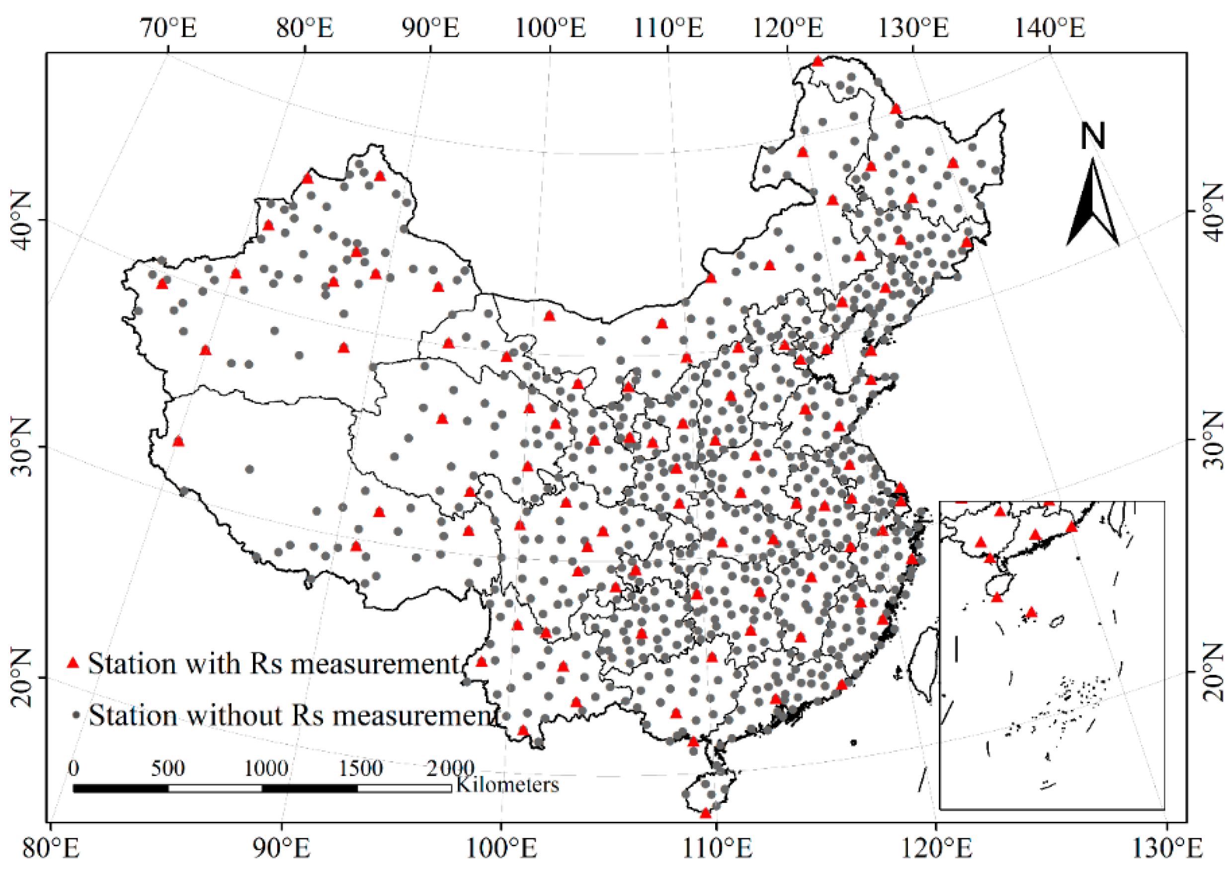
The meteorological data were sourced from the China Meteorological Data Network (http://data.cma.cn/), accessed on 10 May 2024. Since the proportion of outliers and missing values in the climate dataset was relatively low (less than 1%), the method of replacing them with the mean value was adopted to handle these outliers and missing values. In this study, 819 ordinary meteorological stations and 98 stations with solar radiation observation values from 1993 to 2016 were selected (Figure 1). The meteorological data include atmospheric pressure (A), maximum temperature (T_max), minimum temperature (T_min), average temperature (T), relative humidity (RH), precipitation (P), average wind speed (U), sunshine hours (S), maximum sunshine hours (S₀), and zenith radiation (R_a), as well as the daily surface solar radiation (H) of 98 solar radiation stations. Among them, maximum sunshine hours and zenith radiation were calculated from the station latitude (φ), solar constant (G_sc), solar declination (δ) and ordinal number of days within a year. The calculation formulas are as follows [17]:

$$\mathrm{Ra}={\displaystyle \frac{24\cdot 3600\cdot {\mathrm{G}}_{\mathrm{s}\mathrm{c}}}{\pi }}{\mathrm{E}}_0\cdot \left((\cos \phi \cdot \cos \delta \cdot \sin {\mathrm{w}}_{\mathrm{s}})+{\displaystyle \frac{\pi {\mathrm{w}}_{\mathrm{s}}}{180}}\cdot (\sin \phi \cdot \sin \delta )\right)$$

(1)

$${\mathrm{E}}_0=1+0.033\cos ({\displaystyle \frac{2\pi }{365}}\cdot {\mathrm{n}}_{\mathrm{d}\mathrm{a}\mathrm{y}})$$

(2)

$$\delta =23.45\cdot {\displaystyle \frac{\pi }{180}}\cdot \sin \left({\displaystyle \frac{2\pi (284+{\mathrm{n}}_{\mathrm{d}\mathrm{a}\mathrm{y}})}{365}}\right)$$

(3)

$${\mathrm{w}}_{\mathrm{s}}=\arccos \left[-\tan \phi \cdot \tan \delta \right]$$

(4)

Figure 1. Distribution of 98 solar radiation stations and 819 ordinary meteorological stations with long-term observations in China.

The sunset hour angle is not applicable to all computer languages and was calculated using the following formula:

$$\mathrm{X}=1-{\left[\tan (\phi )\right]}^2{\left[\tan (\delta )\right]}^2$$

(5)

$${\mathrm{w}}_{\mathrm{s}}={\displaystyle \frac{\pi }{2}}-\arctan \left[{\displaystyle \frac{-\tan \phi \cdot \tan \delta }{{\mathrm{X}}^{0.5}}}\right]$$

(6)

$${\mathrm{S}}_0={\displaystyle \frac{2}{15}}\cdot {\displaystyle \frac{180}{\pi }}\cdot {\mathrm{w}}_{\mathrm{s}}$$

(7)

where ${\mathrm{G}}_{\mathrm{s}\mathrm{c}}$ is the solar constant (=1367 W⋅m⁻²), ${\mathrm{E}}_0$ is the correction coefficient of the Earth’s orbital eccentricity, ${\mathrm{w}}_{\mathrm{s}}$ is the sunset hour angle (rad), $\phi$ is the latitude (rad), $\delta$ is the solar declination angle (rad), ${\mathrm{n}}_{\mathrm{d}\mathrm{a}\mathrm{y}}$ is the day number in a year, and ${\mathrm{S}}_0$ is the theoretical sunshine hours.

To ensure the reliability and generalizability of the solar radiation estimation models, a rigorous validation procedure was implemented. The dataset was randomly split into three independent subsets: 70% for model training, 15% for hyperparameter tuning and validation, and 15% for independent testing to evaluate the final model performance. A 5-fold cross-validation strategy was applied during the training phase to avoid overfitting and ensure the robustness of the model performance. The model performance was evaluated using four widely recognized metrics: R², RMSE, MAE, and MAPE.

2.2. Solar Radiation Zoning Method

Understanding solar radiation distribution through regional classification based on similar trends is crucial for establishing a comprehensive model that estimates daily radiation levels. To achieve higher classification precision, it was essential to compare multiple clustering techniques and select zoning criterion. Considering that conventional meteorological stations exhibit higher spatial density than solar radiation monitoring sites, this study employed daily relative sunshine duration as the zoning criterion to improve classification accuracy [7]. Three clustering methods—k-means clustering, hierarchical clustering, and bisecting k-means clustering—were implemented to delineate solar radiation zones, with detailed methodologies provided in Appendix A.

2.3. Selection of Sunshine Duration-Based Models

Among empirical models for solar radiation estimation, sunshine-based models continue to be the most widely adopted methodology for R_s quantification [18]. These models have historically encompassed a diverse array of formulations, spanning from the 1980s to the 2010s. Consequently, the following representative models were selected to characterize this methodological progression.

M1: The most used model for predicting global solar radiation based on sunshine hours was developed by Ångström [19] and further modified by Prescott [20], resulting in a linear relationship between the ratio of global solar radiation to extraterrestrial solar radiation and the ratio of daily sunshine hours to the maximum possible sunshine hours (relative sunshine hours). The Angstrom–Prescott model is expressed as follows:

$${\displaystyle \frac{{\mathrm{R}}_{\mathrm{s}}}{{\mathrm{R}}_{\mathrm{a}}}}=\mathrm{a}+\mathrm{b}\cdot {\displaystyle \frac{\mathrm{S}}{{\mathrm{S}}_0}}$$

(8)

where R_s is the total solar radiation; R_a is the extraterrestrial solar radiation, which can be determined as a function of the site latitude, solar declination angle, and Julian day according to the procedure described by Allen [17]; S is the daily sunshine hours (hours); and S₀ is the maximum possible sunshine hours (hours).

M2: BAKIRCI [21] established the relationship between S and S₀:

$${\mathrm{R}}_{\mathrm{s}}=\mathrm{a}\times \mathrm{S}+\mathrm{b}{\mathrm{S}}_0$$

(9)

M3: TOĞRUL [22] established a logarithmic polynomial representation of S₀:

$${\displaystyle \frac{{\mathrm{R}}_{\mathrm{s}}}{{\mathrm{R}}_{\mathrm{a}}}}=\mathrm{a}+\mathrm{b}\ln ({\displaystyle \frac{\mathrm{S}}{{\mathrm{S}}_0}}+1)$$

(10)

M4: Ogelmanet [23] represented R_s using the following polynomial function of s:

$${\displaystyle \frac{{\mathrm{R}}_{\mathrm{s}}}{{\mathrm{R}}_{\mathrm{a}}}}=\mathrm{a}+\mathrm{b}{\displaystyle \frac{\mathrm{S}}{{\mathrm{S}}_0}}+\mathrm{c}({\displaystyle \frac{\mathrm{S}}{{\mathrm{S}}_0}}{)}^2$$

(11)

M5: Bahel [24] derived a polynomial global correlation based on the monthly average daily global solar radiation and sunshine hours data from 48 radiation stations:

$${\displaystyle \frac{{\mathrm{R}}_{\mathrm{s}}}{{\mathrm{R}}_{\mathrm{a}}}}=\mathrm{a}+\mathrm{b}{\displaystyle \frac{\mathrm{S}}{{\mathrm{S}}_0}}+\mathrm{c}({\displaystyle \frac{\mathrm{S}}{{\mathrm{S}}_0}}{)}^2+\mathrm{d}({\displaystyle \frac{\mathrm{S}}{{\mathrm{S}}_0}}{)}^3$$

(12)

M6: The polynomial model proposed by TOĞRUL [25] for estimating R_s is expressed as follows:

$${\mathrm{R}}_{\mathrm{s}}=\mathrm{a}+\mathrm{b}{\mathrm{R}}_{\mathrm{a}}+\mathrm{c}{\displaystyle \frac{\mathrm{S}}{{\mathrm{S}}_0}}$$

(13)

2.4. Correlation Analysis of Meteorological Factors

Random Forest calculates feature importance scores based on each feature’s contribution to the model’s prediction accuracy [2]. Importance is measured by the average reduction in node impurity, specifically the variance of predicted values during decision tree construction. In regression trees, variance typically represents node impurity:

$$\mathrm{V}\mathrm{a}\mathrm{r}(\mathrm{D})={\displaystyle \frac{1}{\mathrm{n}}}{\sum }_{\mathrm{i}=1}^{\mathrm{n}}({\mathrm{x}}_{\mathrm{i}}-\overline{\mathrm{x}}{)}^2$$

(14)

where n is the number of samples, x_i is the value of the i-th sample, and $\overline{\mathrm{x}}$ is the mean value of the samples.

For a node, higher variance of target values indicates greater impurity and data dispersion. When constructing decision trees, the change in node variance before and after splitting is evaluated for each feature [26]. First, the root node’s variance is calculated. Then, for each candidate feature, if the node splits into child nodes based on this feature’s value, the weighted sum of their variances is computed (weights are based on sample proportions). A smaller post-split weighted sum signifies a greater reduction in impurity [27]. Additionally, the Pearson correlation coefficient was applied to analyze the strength and direction of the relationship among meteorological factors.

2.5. Machine Learning and Deep Learning Models

2.5.1. Random Forest (RF)

RF is an ensemble learning technique using multiple decision trees for regression/classification [28]. It employs bagging—training each tree on random data subsets—to balance bias variance and reduce model variance. For regression, it averages predictions from multiple trees. Each tree trains on random data and feature subsets, mitigating overfitting and enhancing generalization. Aggregating trees stabilizes predictions and boosts accuracy. The key parameters include: number of estimators, max features, and max depth [29].

In this study, RF regression was applied to model the nonlinear relationships between meteorological variables and solar radiation. A fixed random state of 42 was used to ensure experimental reproducibility and consistent results across repeated runs. The number of decision trees was retained as the default configuration, which is widely recognized in practical applications to achieve a reliable balance between prediction accuracy and computational efficiency without excessive model complexity. All input features were directly used without additional transformation to avoid introducing unnecessary bias and maintain the physical interpretability of meteorological variables. All models were trained under identical experimental protocols to guarantee a fair and reproducible performance comparison.

2.5.2. Support Vector Machine (SVM)

SVM is a data-driven machine learning method based on statistical learning theory introduced by Russian mathematician Vapnik [30]. SVM is characterized by its simple structure, adaptability, global optimality, fast training speed, and strong generalizability [31,32]. Its success relies on two key technologies for addressing classification and regression problems.

SVM is usually expressed in the following functional form:

$$\mathrm{f}\left(\mathrm{x}\right)=\omega \varphi \left(\mathrm{x}\right)+\mathrm{b}$$

(15)

where ϕ(x) is the high-dimensional feature space transformed from the input vector x; and ω and b are the weight vector and bias, respectively. Since the RBF (Radial Basis Function) nonlinear kernel function has better estimation performance compared to other kernel functions, after trying various kernel functions, the commonly used RBF nonlinear kernel function was adopted:

$${\mathrm{K}}_{\mathrm{r}\mathrm{b}\mathrm{f}}(\mathrm{x},{\mathrm{x}}_{\mathrm{i}})=\exp \left[{\displaystyle \frac{-(\mathrm{x}-{\mathrm{x}}_{\mathrm{i}}{)}^2}{2{\sigma }^2}}\right]$$

(16)

where x and x_i are vectors in the input space and feature vectors calculated from the training/testing datasets, respectively.

In this study, SVM regression was implemented to model the nonlinear relationship between meteorological variables and solar radiation, with the radial basis function kernel selected to capture the complex nonlinear patterns in the data. To ensure optimal model performance and reproducibility, a systematic hyperparameter tuning procedure was conducted: the penalty parameter C (controlling model complexity and generalization) was tested over the range [0.1, 1, 10], and the epsilon-insensitive loss parameter epsilon (defining the margin of tolerance for prediction errors) was tested over the range [0.01, 0.1]. A 5-fold cross-validated grid search was performed on the training set with the negative mean squared error (MSE) as the scoring metric, and the optimal configuration was determined as C = 10 and epsilon = 0.1, which achieved the lowest validation MSE and balanced model fitting and generalizability. The input features were standardized using StandardScaler to eliminate dimensional differences.

2.5.3. Extreme Gradient Boosting (XGB)

The Gradient Boosting Decision Tree (GBDT) algorithm employs gradient descent to create new trees based on previous ones, aiming to minimize the objective function [33]. The XGB algorithm is built upon GBDT and is widely used for classification and regression tasks. By adding regression trees, the model iteratively splits features and learns from each internal node’s data to generate new CART trees that fit the residuals of prior models [34]. It tracks the total number of trees in training and weights each tree’s results to produce the final predicted value [35]. Additionally, XGB employs a second-order Taylor expansion to accelerate convergence and enhance prediction accuracy [36]. The predicted value of the i-th sample in the t-th iteration is given by:

$${\widehat{\mathrm{y}}}_{\mathrm{i}}^{\left(\mathrm{t}\right)}={\widehat{\mathrm{y}}}_{\mathrm{i}}^{(\mathrm{t}-1)}+{\mathrm{f}}_{\mathrm{t}}({\mathrm{x}}_{\mathrm{i}})$$

(17)

where ${\widehat{\mathrm{y}}}_{\mathrm{i}}^{\left(\mathrm{t}\right)}$ is the predicted value of sample i er the t-th iteration, ${\widehat{\mathrm{y}}}_{\mathrm{i}}^{(\mathrm{t}-1)}$ is the predicted value of the (t−1)-th tree, ${\mathrm{f}}_{\mathrm{t}}\left({\mathrm{x}}_{\mathrm{i}}\right)$ is the model of the t-th tree, and ${\mathrm{x}}_{\mathrm{i}}$ is the input value.

The form of the XGB objective function is as follows:

$$\mathrm{O}\mathrm{b}{\mathrm{j}}^{\left(\mathrm{t}\right)}={\sum }_{\mathrm{j}=1}^{\mathrm{n}}\mathrm{l}({\mathrm{y}}_{\mathrm{i}},{\widehat{\mathrm{y}}}_{\mathrm{i}}^{\left(\mathrm{t}\right)})+\Omega ({\mathrm{f}}_{\mathrm{t}})+\mathrm{c}$$

(18)

where $\mathrm{l}({\mathrm{y}}_{\mathrm{i}},{\widehat{\mathrm{y}}}_{\mathrm{i}}^{\left(\mathrm{t}\right)})$ is the loss function of the model, ${\mathrm{y}}_{\mathrm{i}}$ is the true value of the i-th sample, n is the total number of samples, $\Omega \left({\mathrm{f}}_{\mathrm{t}}\right)$ is the regularization term for the complexity of the t-th tree, and c is the offset constant term of the initial predicted value of the model.

XGBoost regression was implemented to capture the complex nonlinear and hierarchical relationships between meteorological variables and solar radiation. To ensure optimal model performance and reproducibility, a systematic hyperparameter tuning procedure was conducted: the maximum tree depth, controlling model complexity, was tested over the range [3,5,7], and the learning rate (eta), controlling gradient update step size, was tested over the range [0.01, 0.1, 0.3], with the regression objective set to reg:squarederror for solar radiation prediction. A 5-fold cross-validated grid search was performed on the training set with the negative mean squared error (MSE) as the scoring metric, and the optimal configuration was determined based on the lowest validation MSE to balance fitting performance and generalization ability. The dataset was split with a fixed random state to ensure consistency, and all training processes followed identical protocols to guarantee fair and reproducible performance comparisons with other models.

2.5.4. Long Short-Term Memory Network (LSTM)

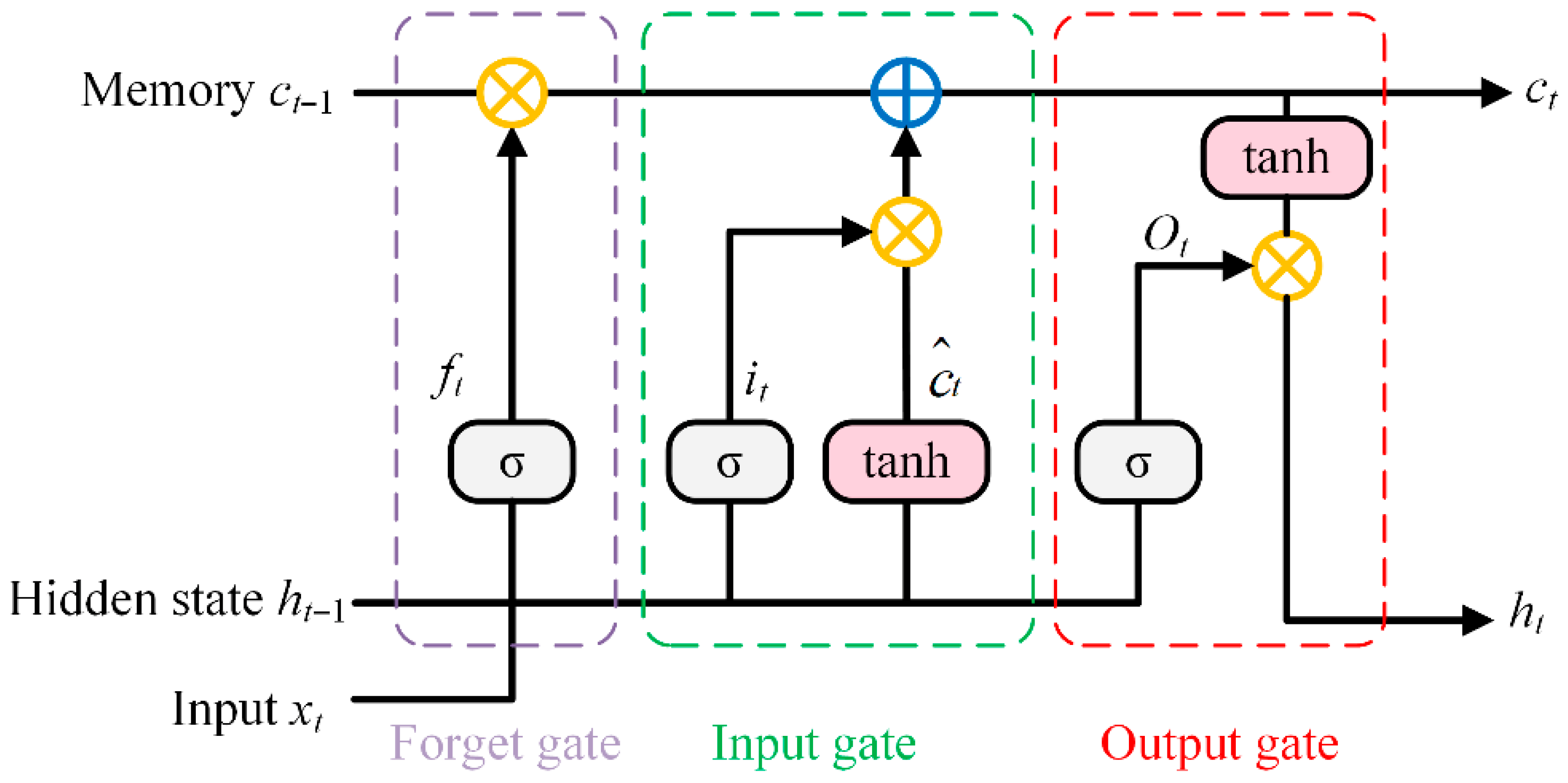
Recurrent Neural Networks (RNNs) are popular deep learning models for time series prediction [37]. Their key feature is network delay recursion, allowing the output of one step to be used as input for the next. However, RNNs struggle with capturing long-term dependencies due to vanishing gradients. To overcome this, Sepp and Schmidhuber [38] introduced Long Short-Term Memory Networks (LSTMs), which use memory cells and gating mechanisms to retain long-term information [39]. The LSTM structure consists of an input gate, a forget gate, a cell memory, and an output gate that manages information within the memory block. Figure 2 shows the LSTM cell structure. The calculations of LSTM are as follows:

$${\mathrm{f}}_{\mathrm{t}}=\sigma ({\mathrm{w}}_{\mathrm{f}}\left[{\mathrm{h}}_{\mathrm{t}}-1,{\mathrm{X}}_{\mathrm{t}}\right]+{\mathrm{b}}_{\mathrm{f}})$$

(19)

$${\mathrm{i}}_{\mathrm{t}}=\sigma ({\mathrm{w}}_{\mathrm{i}}\left[{\mathrm{h}}_{\mathrm{t}}-1,{\mathrm{X}}_{\mathrm{t}}\right]+{\mathrm{b}}_{\mathrm{i}})$$

(20)

$${\mathrm{a}}_{\mathrm{t}}=\tan \mathrm{h}({\mathrm{w}}_{\mathrm{a}}\left[{\mathrm{h}}_{\mathrm{t}}-1,{\mathrm{X}}_{\mathrm{t}}\right]+{\mathrm{b}}_{\mathrm{a}})$$

(21)

$${\mathrm{c}}_{\mathrm{t}}={\mathrm{f}}_{\mathrm{t}}\times {\mathrm{c}}_{\mathrm{t}}-1+{\mathrm{i}}_{\mathrm{t}}\times {\mathrm{a}}_{\mathrm{t}}$$

(22)

$${\mathrm{h}}_{\mathrm{t}}={\mathrm{o}}_{\mathrm{t}}\times \tan \mathrm{h}({\mathrm{c}}_{\mathrm{t}})$$

(23)

where ${\mathrm{f}}_{\mathrm{t}}$, ${\mathrm{i}}_{\mathrm{t}},{\mathrm{o}}_{\mathrm{t}}$, and $\sigma$ are the output values of the forget gate, the input gate, the output gate and the activation function, respectively. The output of the LSTM is calculated using Formulas (19)–(23). The error between the resulting data and the data of each input layer is calculated in the last step, and the weights of each gate are updated using an optimization algorithm based on the calculated error.

Figure 2. The function of main LSTM gates.

2.5.5. Gated Recurrent Unit (GRU)

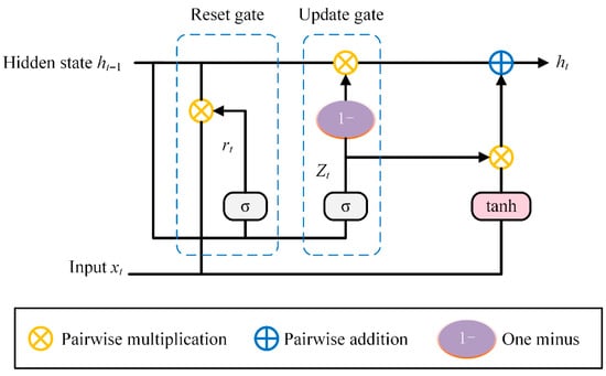
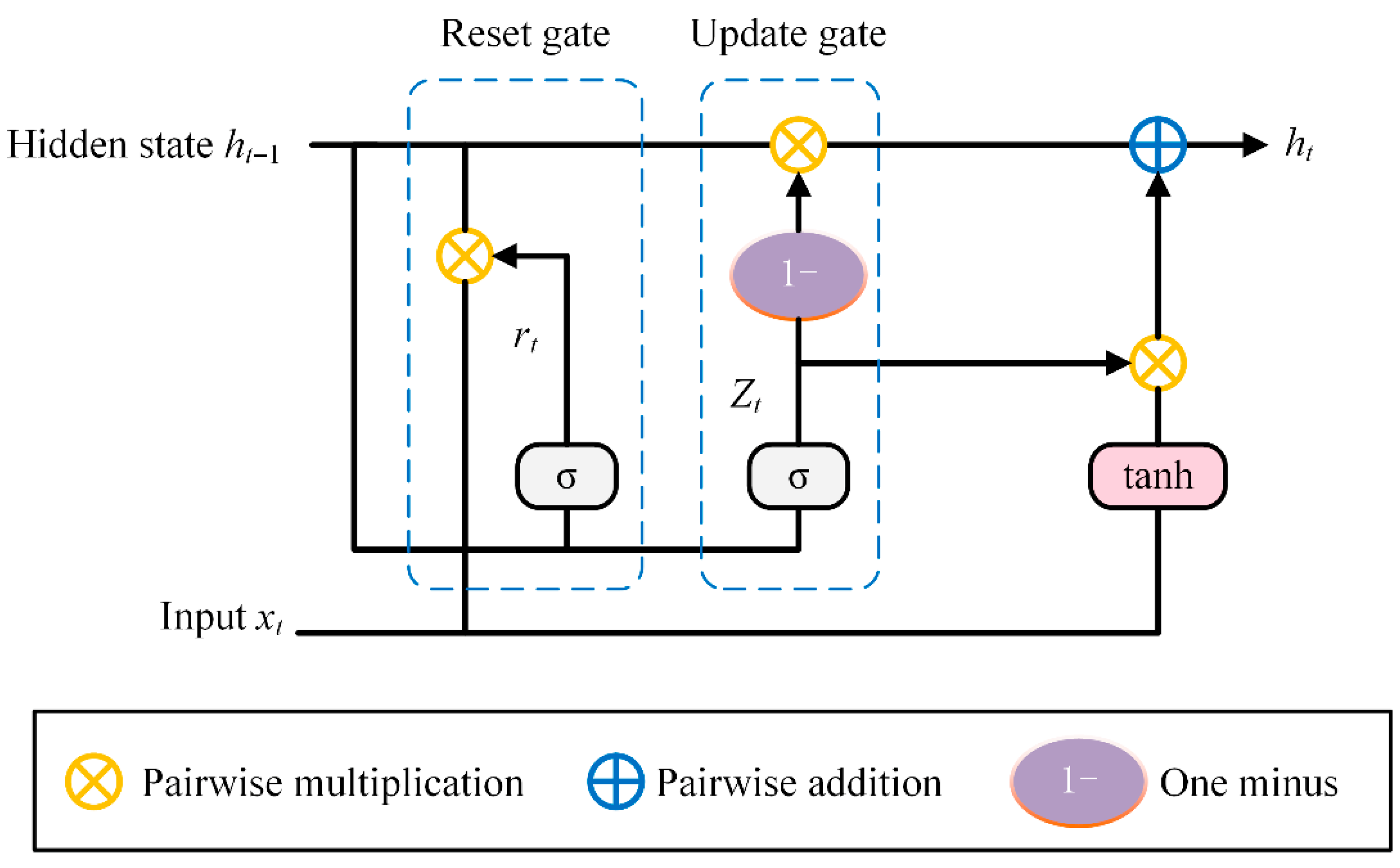
GRU is a variant of Recurrent Neural Networks designed to capture temporal dependencies and patterns in input data. It improves upon Long Short-Term Memory (LSTM) technology [16]. The GRU architecture consists of an update gate (${\mathrm{z}}_{\mathrm{t}}$) and a reset gate (${\mathrm{r}}_{\mathrm{t}}$). The reset gate regulates how much information from the previous state influences the new input ${\mathrm{x}}_{\mathrm{t}}$ for the current hidden layer vector ${\mathrm{h}}_{\mathrm{t}}$. The continuation of ${\mathrm{h}}_{\mathrm{t}-1}$ is controlled by the update gate. With fewer gating mechanisms than LSTM, GRU demonstrates higher computational efficiency [40]. The structure of the GRU cell is given in Figure 3.

Figure 3. Architecture of GRU cell. (The blue dashed boxes highlight the Reset gate and Update gate, the two core components of the GRU structure).

The transformation function formulas for GRUs are as follows:

$${\mathrm{r}}_{\mathrm{t}}=\sigma ({\mathrm{W}}^{\left(\mathrm{r}\right)}{\mathrm{x}}_{\mathrm{t}}+{\mathrm{U}}^{\left(\mathrm{r}\right)}{\mathrm{h}}_{\mathrm{t}-1}+{\mathrm{b}}_{\mathrm{r}})$$

(24)

$${\mathrm{z}}_{\mathrm{t}}=\sigma ({\mathrm{W}}^{\left(\mathrm{z}\right)}{\mathrm{x}}_{\mathrm{t}}+{\mathrm{U}}^{\left(\mathrm{z}\right)}{\mathrm{h}}_{\mathrm{t}-1}+{\mathrm{b}}_{\mathrm{z}})$$

(25)

$${\mathrm{h}}_{\mathrm{t}}={\mathrm{z}}_{\mathrm{t}}\odot {\mathrm{h}}_{\mathrm{t}-1}+(1-{\mathrm{z}}_{\mathrm{t}})\odot {\mathrm{h}}_{\mathrm{t}}^{\prime }$$

(26)

$${\mathrm{h}}_{\mathrm{t}}^{\prime }=\tan \mathrm{h}(\mathrm{W}{\mathrm{x}}_{\mathrm{t}}+{\mathrm{r}}_{\mathrm{t}}\odot \mathrm{U}{\mathrm{h}}_{\mathrm{t}-1}+{\mathrm{b}}_{\mathrm{h}})$$

(27)

where ${\mathrm{W}}^{\left(\mathrm{r}\right)}$ and ${\mathrm{U}}^{\left(\mathrm{r}\right)}$ represent the weight matrices of the input layer and the hidden layer, respectively; and ${\mathrm{b}}_{\mathrm{r}}$ represents the bias term of the reset gate. ${\mathrm{W}}^{\left(\mathrm{z}\right)}$ and ${\mathrm{U}}^{\left(\mathrm{z}\right)}$ represent the weight matrices of the input layer and the hidden layer, respectively; and ${\mathrm{b}}_{\mathrm{z}}$ represents the bias term of the update gate. ${\mathrm{b}}_{\mathrm{h}}$ represents the corresponding bias of the current hidden layer vector.

In this study, LSTM and GRU share substantially consistent parameter configurations. The input time step was set to 12. The hyperbolic tangent (tanh) activation function was employed, as it remains one of the most widely used choices in neural networks. The mean squared error (MSE) between observed and predicted values served as the loss function. The network was trained using the Adam optimization algorithm to minimize MSE, with an initial learning rate of 0.0001, a batch size of 64, and 100 epochs.

2.6. Statistical Indicators

Four statistical indicators were used to evaluate the estimation accuracy of each model, including the coefficient of determination (R²), root mean squared error (RMSE), normalized root mean squared error (NRMSE), and mean absolute error (MAE):

$${\mathrm{R}}^2={{\displaystyle \frac{\left[{\sum }_{\mathrm{i}=1}^{\mathrm{n}}\left({\mathrm{X}}_{\mathrm{i}}-\overline{\mathrm{X}}\right)\left({\mathrm{Y}}_{\mathrm{i}}-\overline{\mathrm{Y}}\right)\right]}{{\sum }_{\mathrm{i}=1}^{\mathrm{n}}{\left({\mathrm{X}}_{\mathrm{i}}-\overline{\mathrm{X}}\right)}^2{\sum }_{\mathrm{i}=1}^{\mathrm{n}}{\left({\mathrm{Y}}_{\mathrm{i}}-\overline{\mathrm{Y}}\right)}^2}}}^2$$

(28)

$$\mathrm{R}\mathrm{M}\mathrm{S}\mathrm{E}=\sqrt{{\displaystyle \frac{1}{\mathrm{n}}}{{\sum }_{\mathrm{i}=1}^{\mathrm{n}}\left({\mathrm{Y}}_{\mathrm{i}}-{\mathrm{X}}_{\mathrm{i}}\right)}^2}$$

(29)

$$\mathrm{N}\mathrm{R}\mathrm{M}\mathrm{S}\mathrm{E}={\displaystyle \frac{\sqrt{\frac{1}{\mathrm{n}}{{\sum }_{\mathrm{i}=1}^{\mathrm{n}}\left({\mathrm{Y}}_{\mathrm{i}}-{\mathrm{X}}_{\mathrm{i}}\right)}^2}}{\overline{\mathrm{X}}}}\times 100\%$$

(30)

$$\mathrm{M}\mathrm{A}\mathrm{E}={\displaystyle \frac{1}{\mathrm{n}}}{\sum }_{\mathrm{i}=1}^{\mathrm{n}}\left|{\mathrm{Y}}_{\mathrm{i}}-{\mathrm{X}}_{\mathrm{i}}\right|$$

(31)

where ${\mathrm{X}}_{\mathrm{i}}$ and ${\mathrm{Y}}_{\mathrm{i}}$ are the observed value and the estimated value, respectively; and $\overline{\mathrm{X}}$ and $\overline{\mathrm{Y}}$ are the average values of the observed value and the estimated value, respectively.

In this study, we first established optimal criteria for solar radiation zoning by comparing three clustering methods based on daily relative sunshine duration. Subsequently, we applied empirical models, machine learning models, and deep learning models within each designated solar radiation region. Given China’s vast territory and diverse regional climates, it was essential to calibrate different empirical models using long-term local meteorological data and conduct comparative evaluations with deep learning and machine learning models in estimating solar radiation.

3. Results

3.1. Solar Radiation Zoning

Using daily relative sunshine duration (S/S₀) from 819 stations, three clustering methods—k-means, hierarchical, and bisecting k-means—were applied to divide China into six solar radiation zones. Evaluation metrics (Table 1) showed that k-means clustering outperformed the others, achieving the highest Dunn index (0.058) and silhouette index (0.33), indicating superior intra-cluster cohesion and inter-cluster separation. Hierarchical clustering excelled in Calinski–Harabasz (766.21) and Davies–Bouldin (0.98) indices, reflecting compact and distinct clusters, but k-means was selected for its balanced performance across critical metrics.

Table 1. Evaluation indicators of various solar radiation zoning methods.

Evaluation Indicators	Dunn Index	Silhouette Index	Calinski–Harabasz Index	Davies–Bouldin Index
K-means clustering	0.058	0.231	377.823	1.162
Hierarchical clustering	0.039	0.315	766.213	0.980
Bisecting k-means clustering	0.044	0.304	742.276	1.051

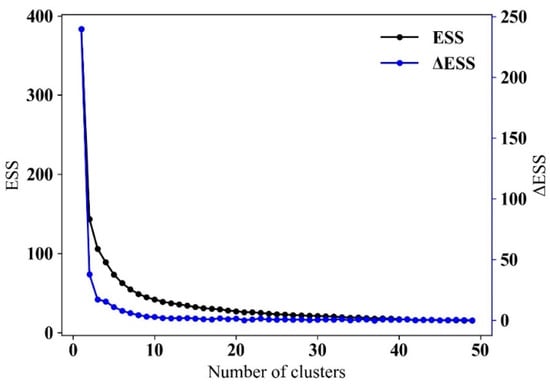
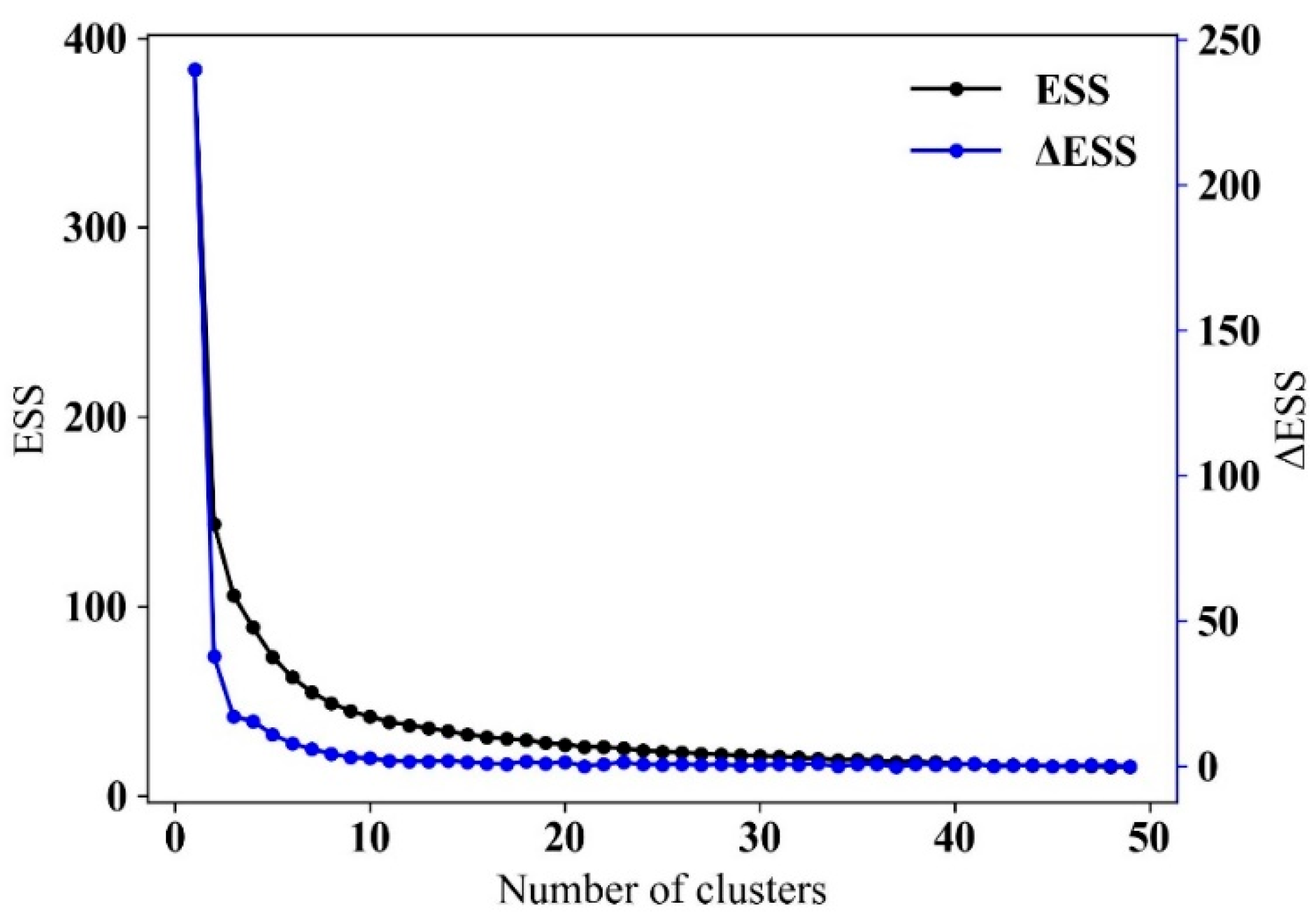
The Effective Similarity Statistic (ESS) analysis (Figure 4) revealed a significant ESS decline from 1 to 6 clusters, which stabilized thereafter, confirming six zones as optimal. To quantitatively and rigorously determine the optimal number of clusters for solar radiation zoning, four widely used validation indices were calculated for cluster numbers ranging from 4 to 8 (Table 2). The results showed that the Silhouette index was relatively high at k = 5 and k = 6, indicating good cluster compactness and separation. The Davies–Bouldin index gradually decreased from k = 4 to k = 7 and reached the minimum at k = 7, while the value at k = 6 was only slightly higher and remained at a low level, reflecting excellent cluster separation. The Calinski–Harabasz index was relatively high at k = 4, 5, and 6, and it decreased as the cluster number increased further. The Dunn index was relatively high at k = 5, 6, and 7, indicating clear inter-cluster boundaries. Considering the overall balance of all four indices, the stability of clustering results, and the actual climatic and geographical heterogeneity across China, k = 6 was determined as the optimal number of solar radiation zones.

Figure 4. The ESS and ΔESS of the number of clusters under S/S₀ criterion.

Table 2. Comparison of clustering validation indices for different numbers of clusters (k = 4 to 8).

Number of Clusters	Silhouette Index	Davies–Bouldin Index	Calinski–Harabasz Index	Dunn Index
4	0.3150	1.1546	899.23	0.0339
5	0.3419	1.0011	857.52	0.0438
6	0.3415	0.9841	809.52	0.0429
7	0.3296	0.9599	810.44	0.0449
8	0.3113	1.0165	788.81	0.0344

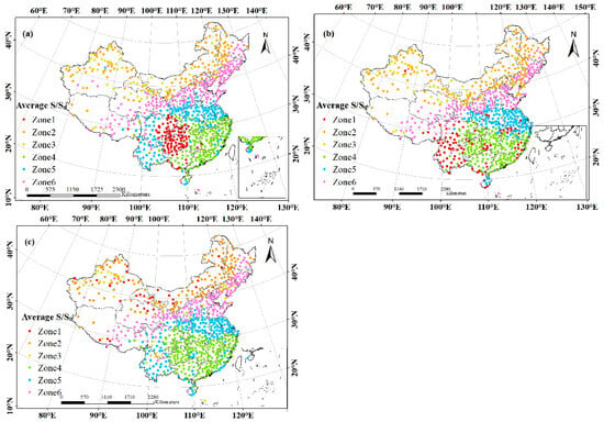
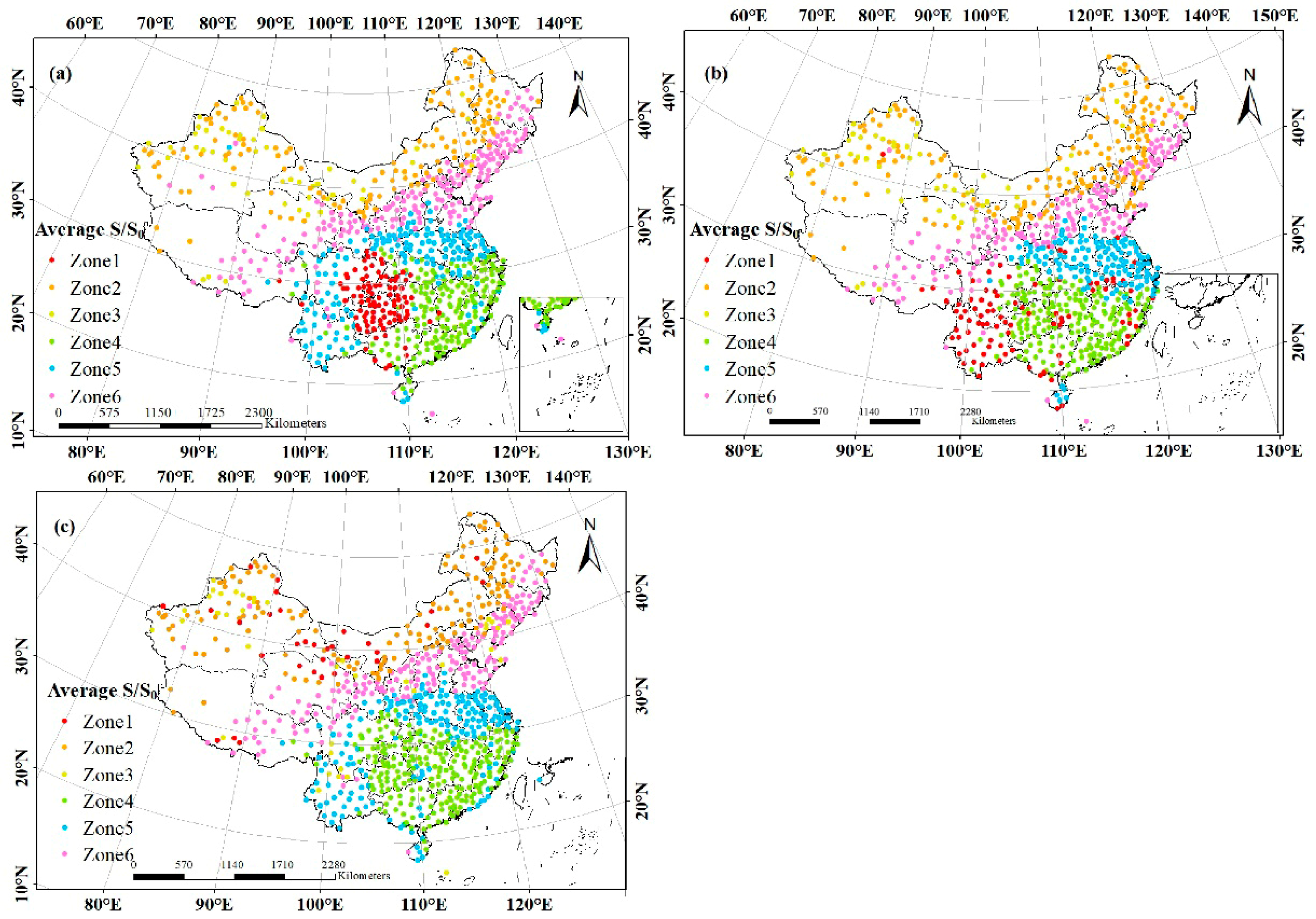
Table 3 summarizes the 98 stations across these zones, with the annual average radiation ranging from 320.028 MJ/m² in Zone 1 to 502.781 MJ/m² in Zone 6. Figure 5 illustrates the geographical distribution of zones, with k-means (Figure 5a) providing the clearest spatial differentiation.

Table 3. Summary of 98 stations in six solar radiation zones.

Zone	Station	Number of Stations	Annual Average Radiation (MJ m2 d−1)
1	Wenjiang, Mianyang, Emeishan, Yichang, Shapingba District, Chongqing, Naxi, Jishou, Guiyang	8	320.028
2	Mohe, Heihe, Hailar, Fuyu, Suolun, Altay, Tacheng, Yanqi, Turpan, Aksu, Kashgar, Hami, Jiuquan, Minqin, Golmud, Erenhot, Wulatezhongqi, Datong, Dongsheng, Yinchuan, Xilinhot, Tongliao, Changchun, Shiquanhe	24	476.134
3	Yining, Urumqi, Ruoqiang, Ejina Banner, Dunhuang, Gangcha	6	502.781
4	Ankang, Wuhan, Changsha, Changning, Guilin, Ganzhou, Baoshan, Hangzhou, Tunxi, Nanchang, Hongjia, Jian’ou, Fuzhou, Guangzhou, Shantou, Nanning, Beihai	17	375.257
5	Houma, Ju County, Hongyuan, Lijiang, Tengchong, Kunming, Jinghong, Mengzi, Zhengzhou, Jinghe, Nanyang, Huai’an, Gushi, Nanjing, Lusi, Hefei, Sanya	17	432.540
6	Jiamusi, Harbin, Hotan, Xining, Yuzhong, Taiyuan, Guyuan, Yan’an, Xifeng Town, Yanji, Chaoyang, Shenyang, Beijing, Tianjin, Leting, Dalian, Fushan, Jinan, Nagqu, Lhasa, Yushu, Guoluo, Chamdo, Ganzi, Panzhihua, Xisha Islands	26	463.863

Figure 5. The annual average S/S of the surface meteorological stations. (a) k-means clustering, (b) hierarchical clustering, (c) bisecting k-means clustering.

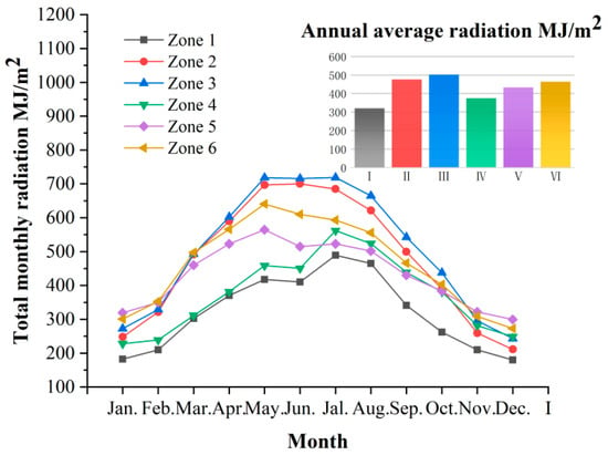
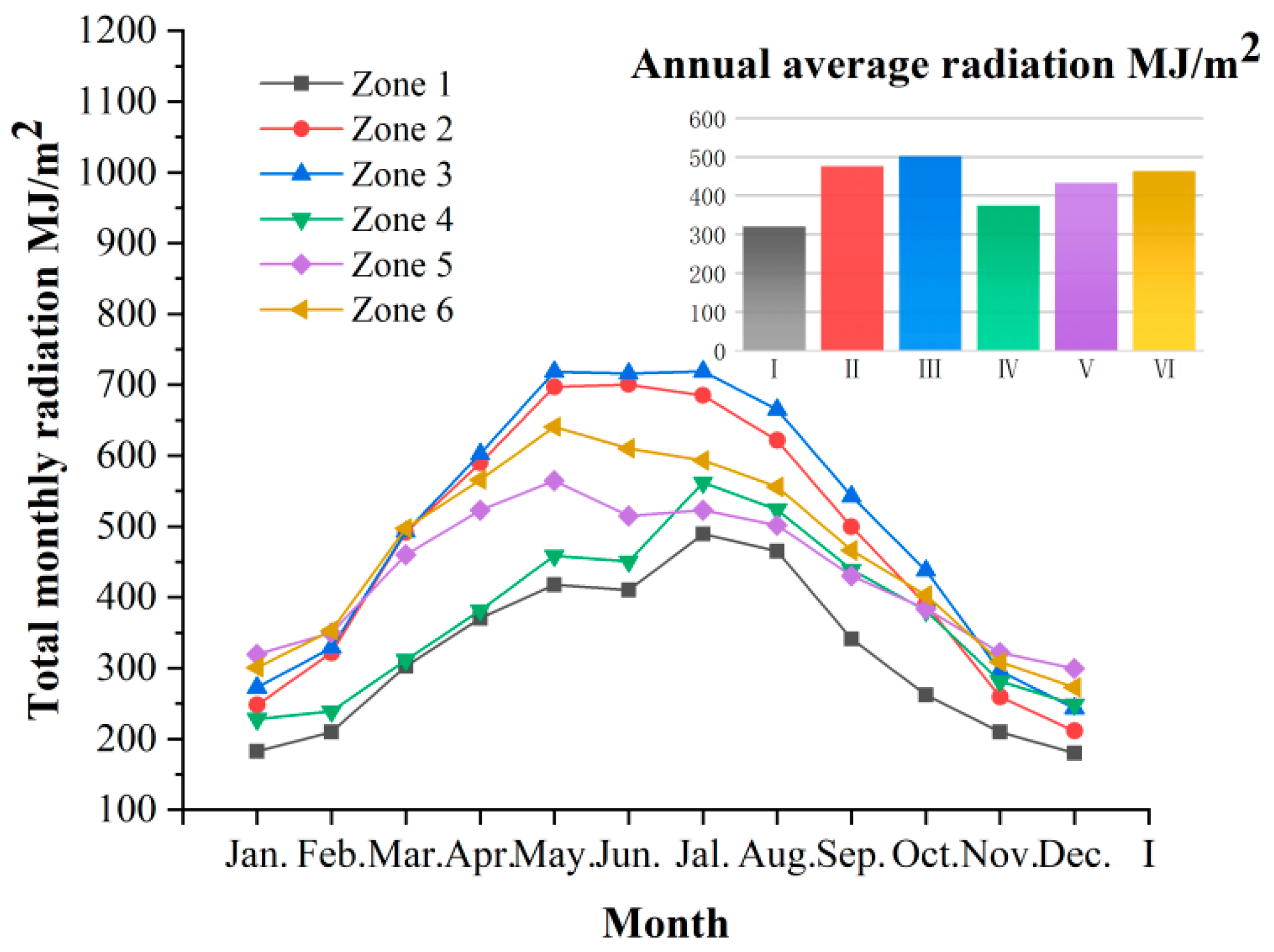
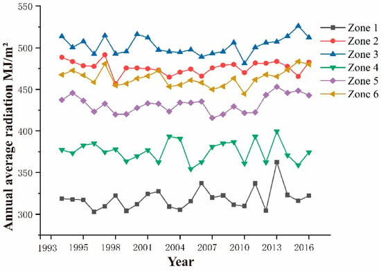
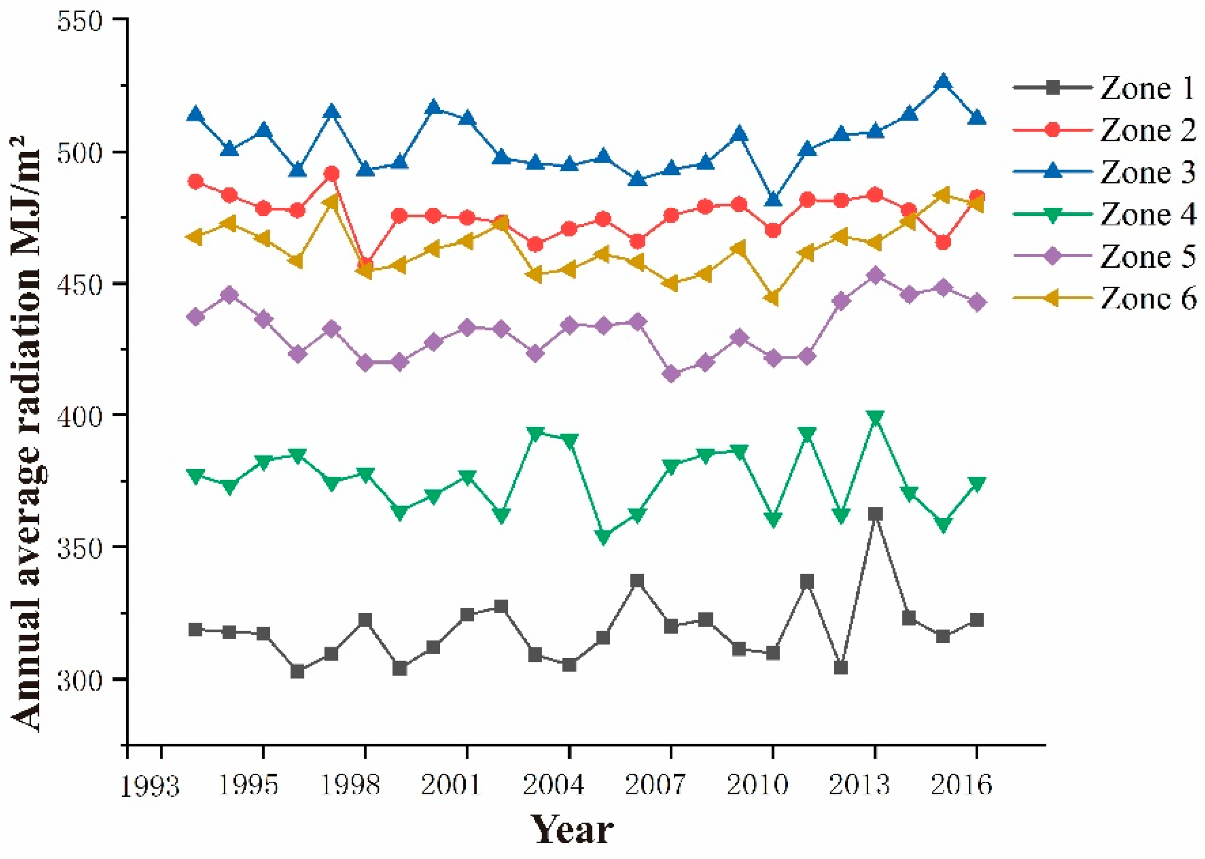
Figure 6 illustrates the monthly and annual average radiation changes across six regions. The monthly average radiation initially rose and then fell, peaking in summer (May to August), with region 3 reaching a maximum of 623.68 in May. Figure 7 presents multi-year trends in annual average radiation, revealing significant fluctuations among regions. Dividing solar radiation into six regions effectively accounted for terrain influences and overall solar climate variations.

Figure 6. Monthly cumulative radiation in six solar radiation zones.

Figure 7. Annual radiation in six solar radiation zones.

3.2. Importance and Correlations of Climatic Factors

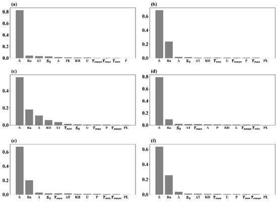
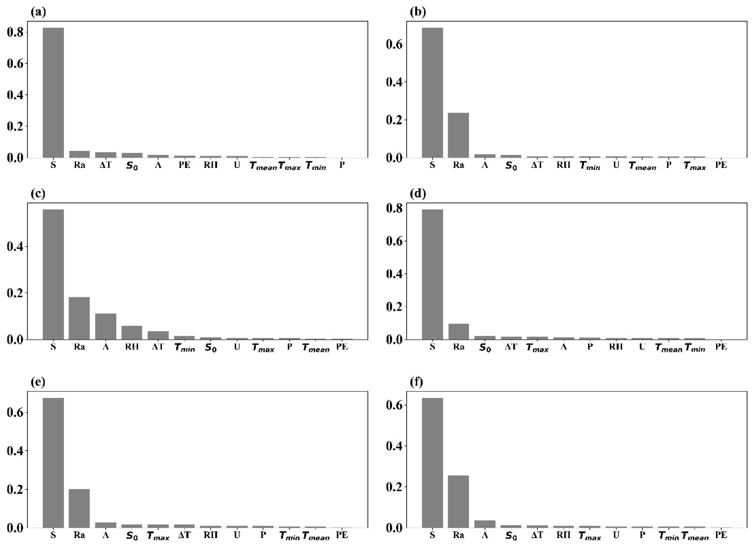
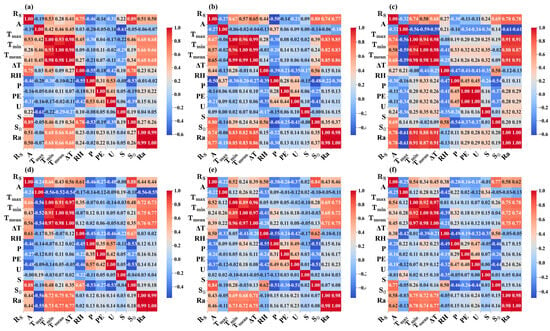
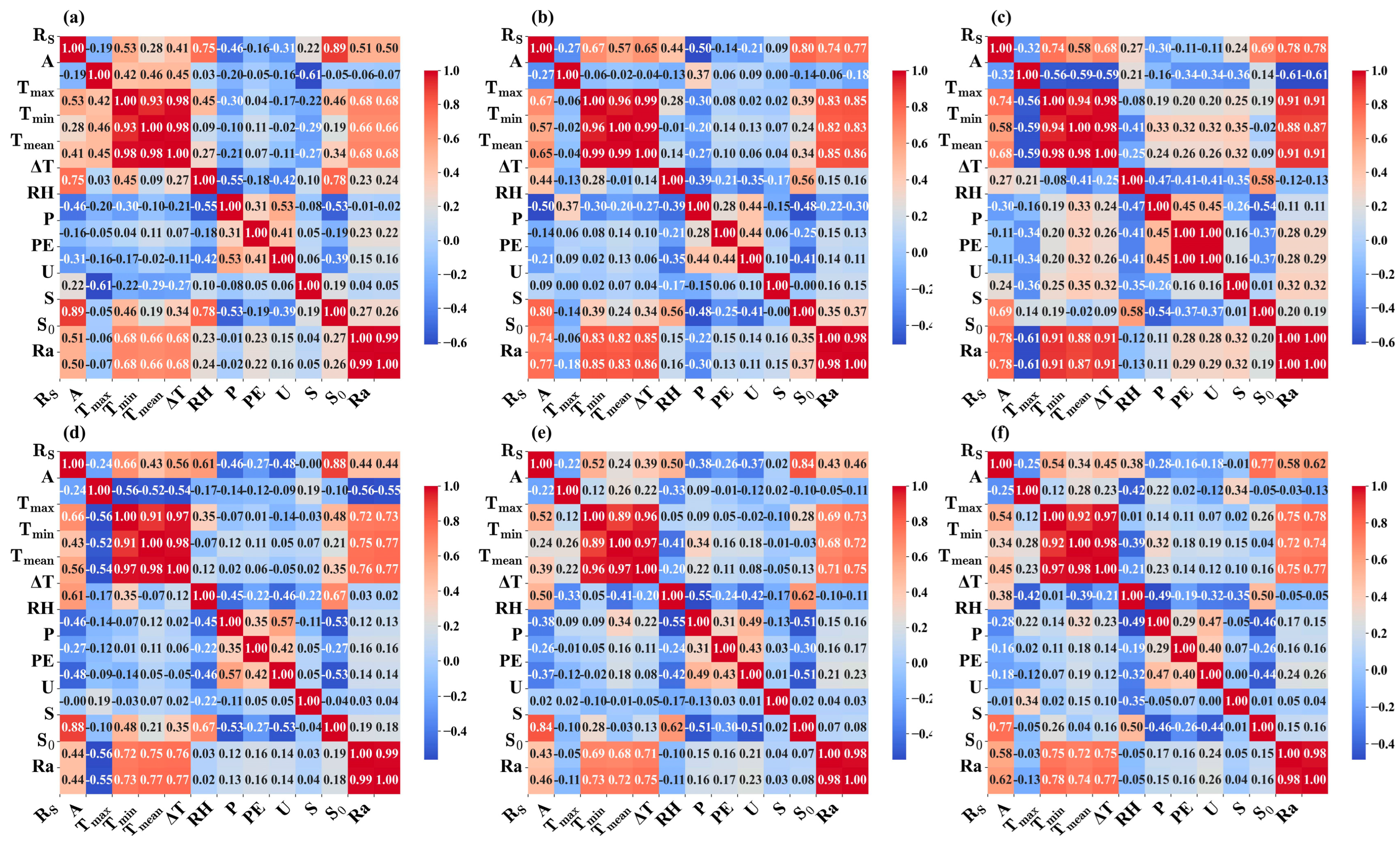
The feature importance scores of each climatic factor on solar radiation were calculated (Figure 8), and the correlation between these climatic factors and solar radiation across six distinct solar radiation regions was analyzed (Figure 9). In the Pearson correlation plot, a deeper shade of red or blue indicates a strong correlation, while lighter shades signify weaker correlations. By integrating the correlation coefficients and feature importance, several meteorological factors that exert significant influence on solar radiation were identified in various regions. In terms of feature importance scores, sunshine hours emerged as having the most substantial impact on solar radiation. With the exception of Radiation Region 3, the feature importance score for sunshine hours approached 0.8. In Radiation Zones 1, 4, 5, and 6, the most critical meteorological factors were S, R_a, ΔT, S₀, and T_max. In Radiation Zone 2, the key meteorological factors were S, R_a, T_mean, S₀, and T_max. In Radiation Zone 3, the most sensitive meteorological factors were R_a, ΔT, RH, and T_max.

Figure 8. The importance of each feature on solar radiation across the six solar radiation zones. (a–f) correspond to Zone 1 through Zone 6, respectively.

Figure 9. Correlation coefficient matrix between predictors and predictand in solar radiation zones. (a–f) correspond to Zone 1 through Zone 6, respectively.

The feature importance analysis revealed distinct regional differences in the dominant meteorological variables driving solar radiation across the six zones. In northern high-latitude zones (Zones 1 and 3), S and R_a were the most critical variables, driven by strong seasonal variations in solar elevation angle and cold, dry continental climates that minimize cloud and precipitation interference. In southern monsoon zones (Zones 2 and 6), ΔT and Tmax showed significantly higher importance, attributed to intense convective activity and frequent cloud formation under the East Asian monsoon, where ΔT and Tmax directly reflect solar heating intensity and cloud attenuation. In central and plateau zones (Zones 4 and 5), altitude-related variables (e.g., atmospheric pressure) and relative humidity were more influential, as high elevation reduces atmospheric thickness and scattering, making solar radiation more sensitive to atmospheric transparency and terrain-modulated radiation balance.

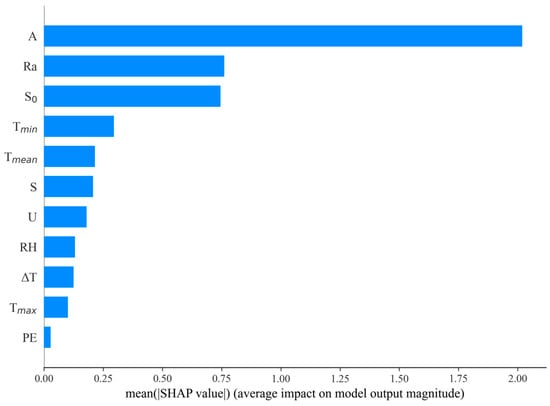
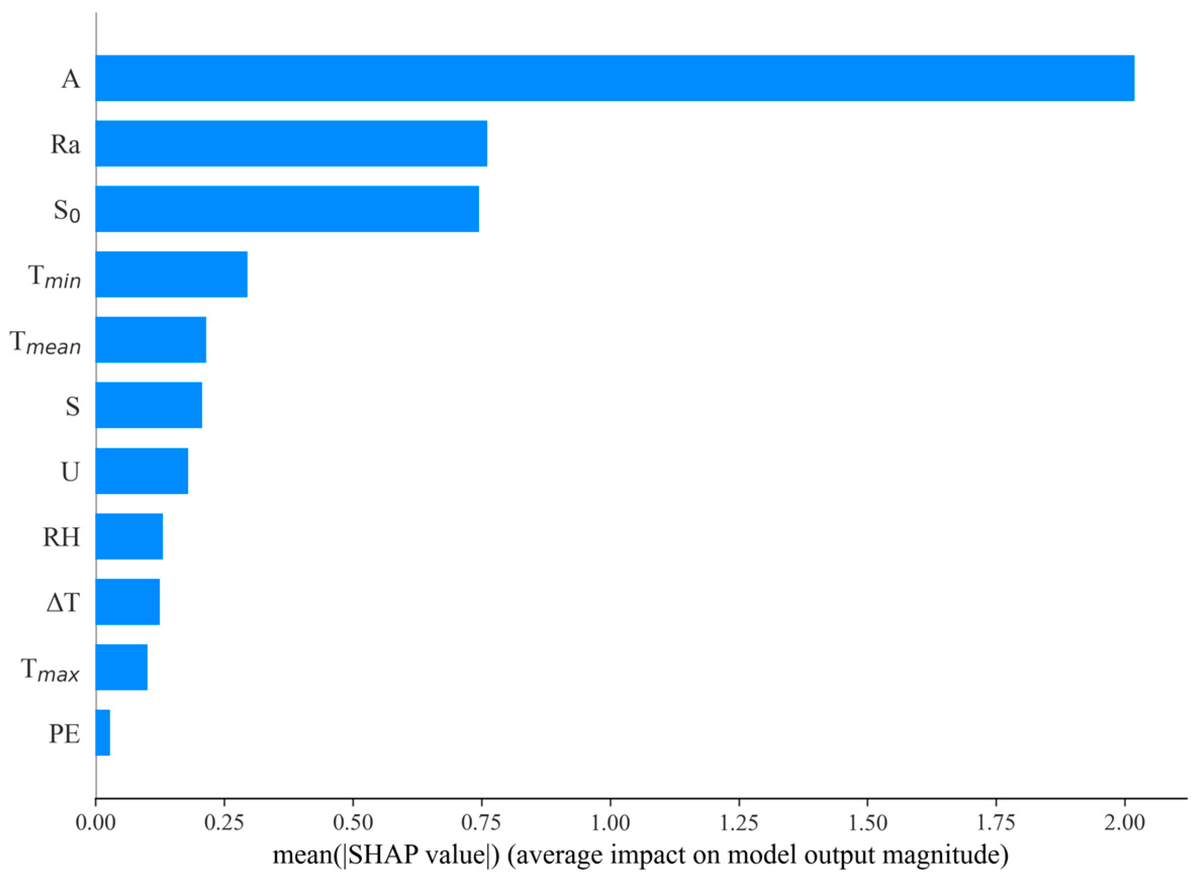
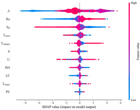
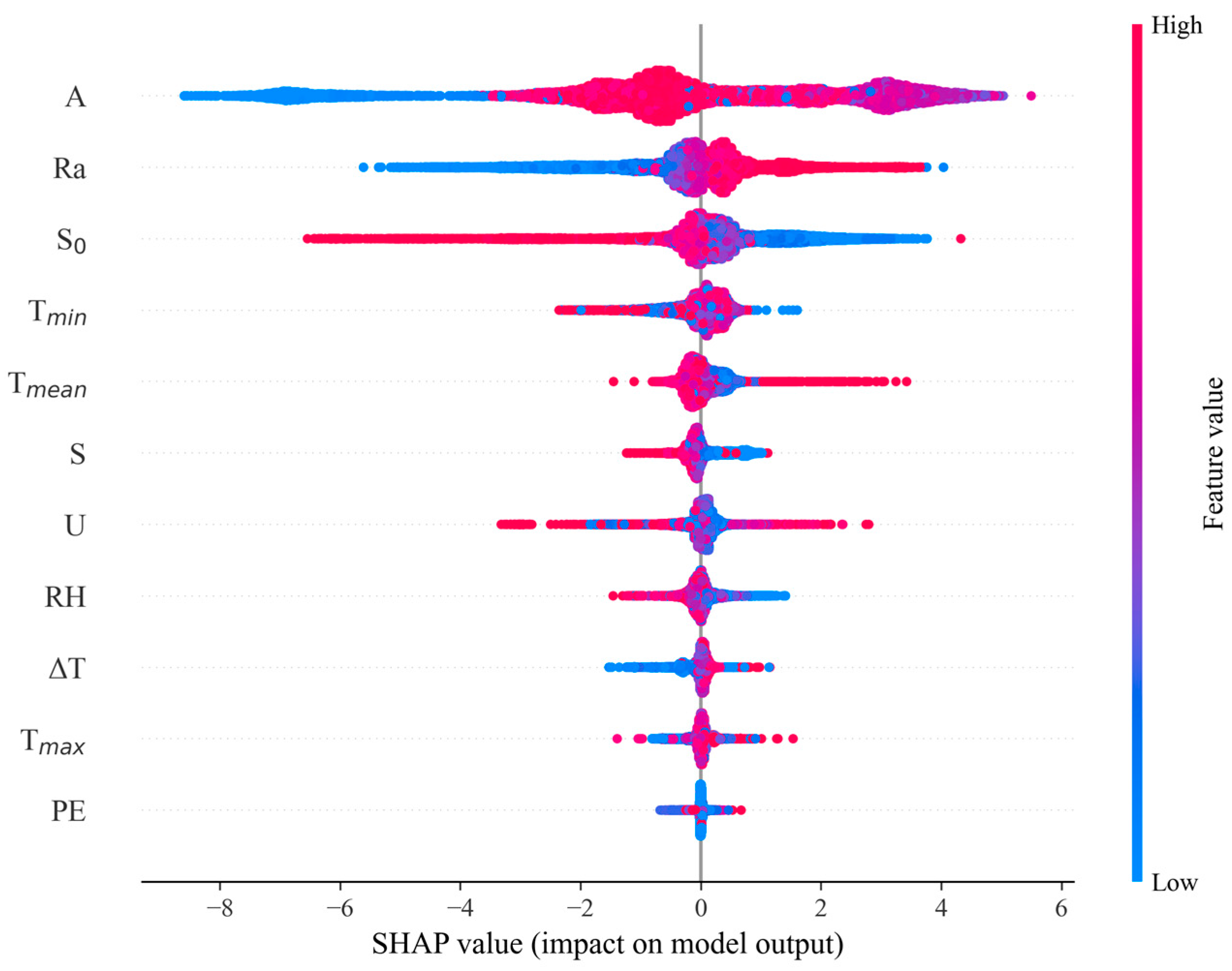
To further clarify the driving mechanisms of solar radiation prediction and quantify input variable contributions, a SHAP analysis was conducted. Figure 10 presents the ranking of feature importance: atmospheric pressure was the dominant driver, followed by extraterrestrial radiation and maximum sunshine duration, with temperature variables, wind speed, and relative humidity having moderate to weak impacts (precipitation is negligible). Figure 11 shows directional effects: high atmospheric pressure, extraterrestrial radiation, and sunshine duration boosted the predicted radiation (consistent with clear sky physics), while high relative humidity and precipitation suppressed it (consistent with cloudy/rainy conditions).

Figure 10. Mean SHAP values showing the average impact of each feature on solar radiation estimation.

Figure 11. SHAP bee swarm plot for feature contribution analysis in solar radiation prediction models.

In summary, the SHAP analysis, feature importance assessment, and Pearson correlation heatmap consistently identified S, Ra, and A as the dominant meteorological drivers of solar radiation across China. These variables exhibited strong positive correlations with solar radiation and exerted the greatest influence on model predictions. Meanwhile, temperature-related factors, wind speed, and relative humidity showed moderate contributions, whereas precipitation had negligible explanatory power. Physically, higher atmospheric pressure, stronger extraterrestrial radiation, and longer sunshine duration correspond to clearer skies and enhanced surface solar radiation, while elevated humidity and precipitation reduce radiation via cloud and precipitation attenuation.

3.3. Performance of Empirical, Machine Learning and Deep Learning Models

To evaluate model stability, a 10-fold repeated random subsampling validation was performed, with the dataset randomly split into 70% training, 15% validation, and 15% testing sets 10 times using different random seeds. All models were retrained and evaluated for each split, and the mean and standard deviation of performance metrics were calculated. The results showed that all models exhibited low performance variability across splits. This confirmed that model performance was not dependent on a specific data partition, demonstrating strong generalizability and robustness for nationwide solar radiation estimation.

China’s vast territory results in significant regional variations in solar radiation, necessitating a robust evaluation of model performance across six radiation zones, as shown in Table 4. A clear hierarchical performance pattern was evident: the deep learning models (LSTM and GRU) outperformed the traditional machine learning models (XGB, SVM, and RF), which in turn were more accurate than the empirical models (M1–M6). This performance gap stemmed from the inherent limitations of empirical models—simple linear formulas cannot fully capture the complex, nonlinear relationships between meteorological factors and solar radiation, while deep learning and machine learning models leverage advanced feature learning and optimization mechanisms to adapt to diverse climatic conditions. LSTM achieved the highest overall accuracy across all zones, with R² values ranging from 0.926 to 0.939, RMSE values ranging between 1.702 and 1.906 MJ/m²/d, and NRMSE values of 0.046–0.058. GRU performed comparably, with only minimal differences from LSTM, confirming that recurrent neural network architectures are well-suited for capturing the temporal dynamics of solar radiation.

Table 4. Performance of the proposed solar radiation estimation models for the investigated areas.

Zone	Site	R2											RMSE											MAE											NRMSE
		M1	M2	M3	M4	M5	M6	RF	SVM	XGB	LSTM	GRU	M1	M2	M3	M4	M5	M6	RF	SVM	XGB	LSTM	GRU	M1	M2	M3	M4	M5	M6	RF	SVM	XGB	LSTM	GRU	M1	M2	M3	M4	M5	M6	RF	SVM	XGB	LSTM	GRU
1	Wenjiang	0.92	0.91	0.93	0.93	0.94	0.92	0.93	0.94	0.93	0.95	0.94	2.04	2.07	1.88	1.85	1.79	1.98	1.94	1.68	1.69	1.52	1.59	1.64	1.67	1.50	1.47	1.41	1.57	1.51	1.25	1.26	1.16	1.21	0.74	0.75	0.68	0.67	0.65	0.72	0.70	0.61	0.61	0.55	0.58
	Mianyang	0.90	0.88	0.91	0.91	0.91	0.90	0.91	0.91	0.92	0.92	0.92	2.23	2.36	2.11	2.10	2.05	2.22	2.11	2.01	1.88	1.94	1.95	1.77	1.89	1.66	1.64	1.58	1.77	1.62	1.51	1.42	1.49	1.50	0.81	0.86	0.77	0.76	0.74	0.81	0.77	0.73	0.68	0.70	0.71
	Emeishan	0.86	0.85	0.85	0.86	0.86	0.86	0.86	0.88	0.89	0.96	0.95	2.63	2.74	2.69	2.64	2.62	2.61	2.55	2.44	2.33	1.55	1.45	1.96	2.03	2.01	1.96	1.96	1.95	1.94	1.79	1.79	1.17	1.27	0.95	0.99	0.97	0.96	0.95	0.95	0.92	0.88	0.84	0.56	0.53
	Yichang	0.89	0.88	0.90	0.90	0.90	0.89	0.93	0.92	0.94	0.95	0.95	2.38	2.42	2.27	2.23	2.19	2.36	1.89	2.12	1.79	1.60	1.60	1.86	1.90	1.74	1.68	1.65	1.84	1.41	1.37	1.24	1.19	1.19	0.86	0.88	0.82	0.81	0.79	0.85	0.68	0.77	0.65	0.58	0.58
	Shapingba	0.85	0.86	0.86	0.86	0.87	0.86	0.87	0.90	0.93	0.90	0.91	2.87	2.86	2.79	2.78	2.75	2.86	2.72	2.51	2.12	2.48	2.41	2.14	2.13	2.07	2.07	2.04	2.13	1.74	1.58	1.56	1.77	1.72	1.04	1.04	1.01	1.01	0.99	1.04	0.98	0.91	0.77	0.90	0.87
	Naxi	0.91	0.91	0.91	0.91	0.92	0.91	0.95	0.97	0.97	0.96	0.96	2.44	2.43	2.35	2.35	2.31	2.39	1.84	1.42	1.51	1.69	1.67	1.90	1.90	1.82	1.83	1.78	1.84	1.43	1.10	1.18	1.31	1.29	0.88	0.88	0.85	0.85	0.84	0.86	0.67	0.51	0.55	0.61	0.61
	Jishou	0.90	0.89	0.91	0.91	0.92	0.90	0.91	0.95	0.96	0.93	0.93	2.15	2.19	2.01	1.95	1.92	2.11	2.02	1.56	1.30	1.79	1.81	1.75	1.78	1.60	1.53	1.48	1.70	1.46	1.10	0.96	1.38	1.40	0.78	0.79	0.73	0.71	0.70	0.76	0.73	0.57	0.47	0.65	0.66
	Guiyang	0.81	0.81	0.82	0.82	0.83	0.82	0.82	0.85	0.86	0.94	0.93	2.84	2.87	2.75	2.73	2.69	2.79	2.80	2.48	2.39	1.91	1.81	2.12	2.14	2.05	2.02	2.00	2.10	1.99	1.67	1.76	1.50	1.40	1.03	1.04	1.00	0.99	0.98	1.01	1.02	0.90	0.86	0.69	0.66
2	Mohe	0.93	0.94	0.94	0.94	0.94	0.94	0.91	0.97	0.96	0.94	0.94	2.05	1.96	2.01	2.01	2.01	2.02	2.38	1.34	1.58	2.03	1.98	1.42	1.26	1.40	1.40	1.40	1.40	1.68	0.99	1.15	1.35	1.32	0.74	0.71	0.73	0.73	0.73	0.73	0.86	0.49	0.57	0.74	0.72
	Heihe	0.92	0.91	0.92	0.92	0.92	0.92	0.91	0.94	0.93	0.93	0.93	2.15	2.28	2.16	2.15	2.13	2.14	2.24	1.82	1.97	2.07	2.08	1.37	1.44	1.39	1.37	1.36	1.36	1.50	1.17	1.29	1.44	1.46	0.78	0.83	0.78	0.78	0.77	0.78	0.81	0.66	0.71	0.75	0.75
	Hailar	0.92	0.95	0.91	0.92	0.92	0.96	0.93	0.96	0.95	0.93	0.93	1.89	1.52	1.97	1.86	1.86	1.34	1.71	1.29	1.39	1.88	1.90	1.41	1.13	1.48	1.39	1.39	1.02	1.30	0.95	1.09	1.36	1.39	0.68	0.55	0.72	0.67	0.67	0.49	0.62	0.47	0.50	0.68	0.69
	Fuyu	0.93	0.93	0.93	0.93	0.93	0.93	0.93	0.94	0.94	0.94	0.94	2.02	2.06	1.98	1.98	1.98	2.00	1.93	1.78	1.88	1.87	1.83	1.27	1.29	1.24	1.24	1.24	1.23	1.33	1.12	1.17	1.29	1.27	0.73	0.75	0.72	0.72	0.72	0.72	0.70	0.65	0.68	0.68	0.66
	Suolun	0.90	0.90	0.89	0.90	0.90	0.90	0.89	0.90	0.91	0.91	0.91	2.58	2.49	2.62	2.58	2.58	2.46	2.59	2.48	2.31	2.28	2.28	1.72	1.58	1.77	1.72	1.72	1.52	1.70	1.46	1.49	1.50	1.51	0.93	0.90	0.95	0.93	0.94	0.89	0.94	0.90	0.84	0.83	0.83
	Altay	0.84	0.85	0.83	0.84	0.84	0.86	0.84	0.87	0.91	0.93	0.94	3.14	3.04	3.19	3.14	3.13	2.87	3.13	2.97	2.47	2.25	2.17	2.47	2.43	2.51	2.46	2.46	2.33	2.42	2.15	1.95	1.63	1.56	1.14	1.10	1.16	1.14	1.13	1.04	1.13	1.08	0.89	0.82	0.79
	Tacheng	0.91	0.92	0.91	0.91	0.91	0.93	0.93	0.95	0.95	0.92	0.92	2.30	2.22	2.34	2.31	2.31	2.07	2.02	1.72	1.75	2.47	2.45	1.76	1.72	1.80	1.77	1.77	1.61	1.50	1.32	1.34	1.76	1.74	0.83	0.80	0.85	0.84	0.84	0.75	0.73	0.62	0.63	0.90	0.89
	Yanqi	0.95	0.96	0.94	0.95	0.95	0.95	0.94	0.95	0.97	0.95	0.95	1.98	1.77	2.07	1.97	1.98	1.92	2.07	2.09	1.44	1.88	1.81	1.51	1.34	1.58	1.51	1.52	1.46	1.51	1.23	1.08	1.45	1.40	0.72	0.64	0.75	0.71	0.72	0.69	0.75	0.76	0.52	0.68	0.66
	Turpan	0.94	0.94	0.93	0.94	0.94	0.94	0.94	0.96	0.96	0.95	0.96	2.06	2.02	2.12	2.07	2.01	2.07	2.01	1.56	1.59	1.83	1.73	1.45	1.45	1.49	1.46	1.41	1.45	1.40	1.07	1.08	1.34	1.28	0.75	0.73	0.77	0.75	0.73	0.75	0.73	0.57	0.58	0.66	0.63
	Aksu	0.94	0.95	0.93	0.95	0.95	0.94	0.93	0.94	0.95	0.93	0.93	1.69	1.58	1.82	1.64	1.63	1.69	1.85	1.70	1.54	1.86	1.91	1.28	1.15	1.38	1.23	1.22	1.27	1.37	1.16	1.12	1.30	1.37	0.61	0.57	0.66	0.59	0.59	0.61	0.67	0.62	0.56	0.67	0.69
	Kashgar	0.93	0.94	0.92	0.93	0.93	0.93	0.92	0.94	0.94	0.94	0.95	2.03	1.87	2.12	1.99	1.99	1.96	2.02	1.62	1.71	1.86	1.80	1.45	1.36	1.51	1.44	1.44	1.39	1.53	1.20	1.26	1.42	1.37	0.74	0.68	0.77	0.72	0.72	0.71	0.73	0.59	0.62	0.67	0.65
	Hami	0.89	0.90	0.88	0.89	0.89	0.89	0.88	0.92	0.90	0.92	0.92	3.10	2.95	3.17	3.08	3.08	3.05	3.22	2.63	2.88	2.23	2.16	2.32	2.25	2.35	2.34	2.34	2.33	2.37	1.96	2.15	1.57	1.51	1.12	1.07	1.15	1.12	1.12	1.10	1.17	0.95	1.04	0.81	0.78
	Jiuquan	0.90	0.90	0.88	0.90	0.90	0.90	0.89	0.90	0.91	0.92	0.92	2.40	2.37	2.53	2.32	2.30	2.37	2.51	2.40	2.30	2.10	2.12	1.82	1.80	1.94	1.74	1.70	1.81	1.85	1.56	1.69	1.50	1.54	0.87	0.86	0.92	0.84	0.83	0.86	0.91	0.87	0.83	0.76	0.77
	Minqin	0.96	0.96	0.95	0.96	0.96	0.96	0.95	0.96	0.96	0.95	0.95	1.49	1.57	1.58	1.48	1.47	1.49	1.69	1.45	1.40	1.59	1.59	1.07	1.11	1.16	1.06	1.05	1.07	1.25	0.94	0.94	1.13	1.11	0.54	0.57	0.57	0.54	0.53	0.54	0.61	0.53	0.51	0.58	0.57
	Golmud	0.96	0.96	0.96	0.96	0.96	0.96	0.95	0.96	0.96	0.96	0.96	1.37	1.42	1.43	1.38	1.37	1.37	1.63	1.44	1.36	1.37	1.43	1.03	1.06	1.08	1.03	1.01	1.02	1.24	1.03	0.99	1.02	1.05	0.50	0.51	0.52	0.50	0.50	0.50	0.59	0.52	0.49	0.50	0.52
	Erenhot	0.95	0.95	0.95	0.95	0.95	0.96	0.94	0.94	0.95	0.91	0.91	1.88	1.86	1.91	1.88	1.88	1.81	2.14	2.10	1.98	2.38	2.32	1.45	1.43	1.47	1.45	1.45	1.43	1.63	1.49	1.45	1.62	1.58	0.68	0.67	0.69	0.68	0.68	0.66	0.78	0.76	0.72	0.86	0.84
	Urad Middle Banner	0.96	0.95	0.96	0.96	0.96	0.96	0.95	0.93	0.96	0.97	0.97	1.59	1.73	1.61	1.58	1.58	1.59	1.79	2.05	1.50	1.41	1.42	1.12	1.19	1.15	1.12	1.12	1.13	1.27	1.21	1.09	1.02	1.03	0.58	0.63	0.58	0.57	0.57	0.58	0.65	0.74	0.54	0.51	0.51
	Datong	0.95	0.94	0.95	0.95	0.95	0.95	0.92	0.94	0.94	0.92	0.92	1.65	1.79	1.65	1.64	1.63	1.65	2.03	1.90	1.91	2.14	2.21	1.23	1.32	1.22	1.22	1.20	1.23	1.53	1.37	1.33	1.60	1.64	0.60	0.65	0.60	0.59	0.59	0.60	0.73	0.69	0.69	0.78	0.80
	Dongsheng	0.96	0.95	0.96	0.96	0.96	0.96	0.94	0.96	0.95	0.93	0.93	1.60	1.74	1.60	1.59	1.57	1.60	1.82	1.56	1.68	2.02	2.05	1.20	1.27	1.21	1.20	1.18	1.19	1.40	1.17	1.25	1.48	1.51	0.58	0.63	0.58	0.58	0.57	0.58	0.66	0.57	0.61	0.73	0.74
	Yinchuan	0.90	0.90	0.89	0.90	0.90	0.91	0.90	0.92	0.92	0.94	0.94	2.32	2.23	2.35	2.32	2.31	2.20	2.28	2.03	2.14	1.76	1.76	1.73	1.64	1.75	1.73	1.72	1.65	1.73	1.51	1.60	1.28	1.29	0.84	0.81	0.85	0.84	0.84	0.80	0.83	0.74	0.78	0.64	0.64
	Xilinhot	0.94	0.95	0.94	0.94	0.94	0.95	0.93	0.95	0.96	0.95	0.95	1.80	1.76	1.84	1.80	1.80	1.74	1.99	1.71	1.58	1.78	1.78	1.27	1.25	1.30	1.27	1.27	1.25	1.48	1.17	1.15	1.33	1.33	0.65	0.64	0.67	0.65	0.65	0.63	0.72	0.62	0.57	0.64	0.64
	Tongliao	0.88	0.88	0.88	0.88	0.88	0.88	0.86	0.88	0.89	0.97	0.97	2.36	2.34	2.36	2.36	2.36	2.36	2.52	2.28	2.22	1.35	1.37	1.69	1.64	1.69	1.69	1.69	1.68	1.86	1.66	1.62	0.95	0.97	0.86	0.85	0.85	0.85	0.85	0.85	0.91	0.83	0.80	0.49	0.50
	Changchun	0.92	0.92	0.91	0.92	0.92	0.92	0.89	0.91	0.93	0.95	0.94	2.32	2.35	2.37	2.32	2.32	2.32	2.55	2.31	2.00	1.79	1.79	1.50	1.55	1.55	1.50	1.50	1.48	1.77	1.51	1.38	1.23	1.24	0.84	0.85	0.86	0.84	0.84	0.84	0.92	0.84	0.72	0.65	0.65
	Shiquanhe	0.94	0.93	0.94	0.94	0.94	0.94	0.91	0.93	0.93	0.95	0.96	1.55	1.64	1.60	1.54	1.53	1.55	1.94	1.69	1.63	1.44	1.54	1.09	1.15	1.13	1.09	1.08	1.09	1.34	1.13	1.12	1.14	1.16	0.56	0.59	0.58	0.56	0.56	0.56	0.70	0.61	0.59	0.52	0.56
3	Yining	0.94	0.95	0.94	0.95	0.95	0.95	0.96	0.95	0.96	0.94	0.94	1.99	1.89	2.12	1.96	1.95	1.91	1.81	1.88	1.76	2.14	2.18	1.43	1.38	1.52	1.42	1.41	1.42	1.36	1.40	1.37	1.48	1.52	0.72	0.68	0.77	0.71	0.71	0.69	0.66	0.68	0.64	0.78	0.79
	Urumqi	0.94	0.95	0.94	0.94	0.94	0.95	0.95	0.93	0.95	0.91	0.91	2.71	2.53	2.82	2.73	2.71	2.61	2.47	2.98	2.44	2.63	2.57	1.91	1.80	2.00	1.92	1.92	1.91	1.87	1.90	1.78	1.90	1.84	0.98	0.91	1.02	0.99	0.98	0.95	0.89	1.08	0.88	0.95	0.93
	Ruoqiang	0.96	0.96	0.95	0.96	0.96	0.96	0.94	0.96	0.97	0.93	0.92	1.39	1.40	1.46	1.39	1.38	1.39	1.74	1.41	1.17	1.93	2.01	1.03	1.04	1.10	1.02	1.02	1.03	1.30	0.95	0.87	1.32	1.41	0.50	0.51	0.53	0.50	0.50	0.51	0.63	0.51	0.42	0.70	0.73
	Ejina Banner	0.95	0.95	0.95	0.95	0.95	0.95	0.91	0.96	0.96	0.94	0.94	1.69	1.71	1.68	1.68	1.68	1.68	2.26	1.64	1.56	1.90	1.85	1.31	1.27	1.29	1.30	1.30	1.27	1.66	1.18	1.19	1.34	1.32	0.61	0.62	0.61	0.61	0.61	0.61	0.82	0.59	0.56	0.69	0.67
	Dunhuang	0.97	0.97	0.96	0.97	0.97	0.97	0.95	0.96	0.97	0.97	0.97	1.44	1.43	1.53	1.44	1.42	1.44	1.79	1.49	1.44	1.35	1.37	1.08	1.04	1.16	1.05	1.03	1.06	1.30	1.03	1.06	0.95	0.97	0.52	0.52	0.56	0.52	0.52	0.52	0.65	0.54	0.52	0.49	0.50
	Gangcha	0.94	0.94	0.94	0.94	0.95	0.94	0.92	0.91	0.90	0.95	0.94	1.54	1.58	1.62	1.55	1.52	1.53	1.75	1.88	1.93	1.49	1.50	1.13	1.14	1.18	1.13	1.11	1.12	1.30	1.27	1.31	1.11	1.11	0.56	0.57	0.59	0.56	0.55	0.55	0.63	0.68	0.70	0.54	0.54
4	Ankang	0.94	0.93	0.94	0.94	0.94	0.94	0.93	0.96	0.96	0.92	0.92	2.01	2.07	1.91	1.91	1.89	2.00	2.02	1.69	1.59	2.28	2.22	1.53	1.57	1.44	1.45	1.44	1.51	1.56	1.18	1.22	1.73	1.67	0.73	0.75	0.69	0.69	0.68	0.72	0.73	0.61	0.58	0.82	0.80
	Wuhan	0.92	0.91	0.93	0.93	0.93	0.92	0.94	0.95	0.95	0.94	0.94	2.14	2.23	2.03	2.03	1.93	2.14	1.89	1.60	1.59	1.70	1.70	1.69	1.77	1.59	1.59	1.50	1.69	1.44	1.19	1.18	1.33	1.33	0.78	0.81	0.74	0.74	0.70	0.77	0.68	0.58	0.58	0.62	0.62
	Changsha	0.88	0.87	0.89	0.89	0.90	0.88	0.92	0.94	0.94	0.95	0.94	2.76	2.88	2.65	2.64	2.57	2.71	2.27	1.94	1.93	1.94	1.63	2.10	2.24	1.99	1.99	1.94	2.08	1.76	1.40	1.38	1.50	1.29	1.00	1.04	0.96	0.96	0.93	0.98	0.82	0.70	0.70	0.70	0.59
	Changning	0.87	0.84	0.88	0.88	0.89	0.87	0.92	0.93	0.93	0.95	0.95	2.08	2.28	1.98	1.95	1.92	2.07	1.64	1.55	1.55	1.56	1.54	1.73	1.91	1.63	1.61	1.57	1.72	1.25	1.14	1.20	1.49	1.59	0.75	0.83	0.72	0.71	0.69	0.75	0.59	0.56	0.56	0.56	0.56
	Guilin	0.89	0.88	0.90	0.90	0.91	0.89	0.89	0.92	0.91	0.96	0.95	3.15	3.20	2.97	2.95	2.87	3.14	3.18	2.71	2.83	1.55	1.53	2.56	2.59	2.41	2.38	2.31	2.55	2.39	2.00	2.17	1.38	1.39	1.14	1.16	1.08	1.07	1.04	1.14	1.15	0.98	1.02	0.56	0.55
	Ganzhou	0.90	0.89	0.90	0.90	0.91	0.90	0.89	0.92	0.93	0.91	0.91	2.06	2.19	2.02	2.03	1.97	2.06	2.16	1.94	1.75	2.09	2.09	1.68	1.78	1.62	1.63	1.59	1.68	1.68	1.43	1.38	1.59	1.61	0.75	0.79	0.73	0.73	0.71	0.75	0.78	0.70	0.63	0.76	0.76
	Baoshan	0.91	0.90	0.92	0.93	0.93	0.91	0.94	0.95	0.95	0.93	0.93	2.25	2.36	2.08	2.02	1.96	2.25	1.88	1.65	1.62	1.90	1.89	1.76	1.85	1.58	1.51	1.44	1.75	1.43	1.29	1.24	1.45	1.44	0.82	0.85	0.75	0.73	0.71	0.81	0.68	0.60	0.59	0.69	0.69
	Hangzhou	0.91	0.89	0.92	0.92	0.92	0.91	0.93	0.94	0.94	0.94	0.93	2.30	2.47	2.19	2.18	2.16	2.29	2.02	1.80	1.82	1.65	1.75	1.84	1.99	1.72	1.71	1.68	1.83	1.56	1.32	1.45	1.30	1.40	0.83	0.89	0.79	0.79	0.78	0.83	0.73	0.65	0.66	0.60	0.63
	Tunxi	0.91	0.90	0.92	0.92	0.93	0.91	0.93	0.94	0.94	0.95	0.95	2.26	2.38	2.12	2.11	2.06	2.26	2.04	1.73	1.75	1.68	1.65	1.74	1.88	1.61	1.61	1.57	1.74	1.62	1.35	1.29	1.34	1.31	0.82	0.86	0.77	0.76	0.75	0.82	0.74	0.63	0.63	0.57	0.91
	Nanchang	0.90	0.90	0.91	0.90	0.91	0.90	0.93	0.93	0.93	0.93	0.93	2.31	2.37	2.28	2.29	2.23	2.31	2.01	1.90	1.80	2.00	2.02	1.69	1.75	1.66	1.67	1.58	1.69	1.54	1.45	1.35	1.47	1.47	0.84	0.86	0.83	0.83	0.81	0.84	0.73	0.69	0.65	0.61	0.90
	Hongjia	0.92	0.91	0.93	0.93	0.94	0.92	0.92	0.93	0.94	0.94	0.95	2.05	2.13	1.89	1.86	1.80	2.04	2.07	1.83	1.65	1.64	1.60	1.60	1.71	1.46	1.44	1.37	1.59	1.62	1.40	1.31	1.25	1.19	0.74	0.77	0.69	0.68	0.65	0.74	0.75	0.66	0.60	0.82	0.92
	Jian’ou	0.89	0.88	0.90	0.90	0.91	0.89	0.93	0.93	0.94	0.94	0.94	2.35	2.46	2.23	2.22	2.17	2.34	1.96	1.89	1.69	1.72	1.70	1.83	1.93	1.74	1.73	1.68	1.83	1.54	1.42	1.25	1.34	1.33	0.85	0.89	0.81	0.80	0.79	0.85	0.71	0.68	0.61	0.62	0.62
	Fuzhou	0.89	0.88	0.91	0.91	0.92	0.89	0.90	0.95	0.94	0.94	0.94	2.63	2.73	2.45	2.39	2.29	2.62	2.49	1.75	1.85	2.14	2.18	2.07	2.15	1.90	1.84	1.73	2.06	1.83	1.32	1.40	1.48	1.52	0.95	0.99	0.89	0.87	0.83	0.95	0.90	0.63	0.67	0.78	0.79
	Guangzhou	0.89	0.89	0.90	0.90	0.91	0.89	0.92	0.95	0.95	0.95	0.95	2.10	2.14	2.01	2.02	1.91	2.06	1.84	1.44	1.42	1.59	1.62	1.65	1.65	1.58	1.61	1.50	1.60	1.43	1.13	1.08	1.14	1.17	0.76	0.78	0.73	0.73	0.69	0.75	0.67	0.52	0.51	0.58	0.59
	Shantou	0.90	0.89	0.90	0.90	0.90	0.90	0.91	0.94	0.95	0.91	0.90	2.21	2.28	2.17	2.18	2.14	2.21	2.06	1.73	1.57	2.04	2.10	1.69	1.73	1.66	1.67	1.64	1.69	1.59	1.32	1.22	1.57	1.60	0.80	0.83	0.79	0.79	0.78	0.80	0.75	0.63	0.57	0.74	0.76
	Nanning	0.90	0.88	0.91	0.91	0.92	0.90	0.91	0.95	0.96	0.94	0.94	2.14	2.29	2.02	2.00	1.93	2.14	2.05	1.46	1.36	1.63	1.63	1.69	1.82	1.56	1.55	1.48	1.69	1.59	1.10	1.04	1.24	1.24	0.78	0.83	0.73	0.72	0.70	0.78	0.74	0.53	0.49	0.59	0.59
	Beihai	0.88	0.87	0.89	0.89	0.89	0.88	0.87	0.90	0.91	0.90	0.90	2.68	2.74	2.56	2.56	2.53	2.68	2.76	2.30	2.19	2.39	2.41	2.16	2.21	2.06	2.05	2.02	2.17	2.14	1.85	1.76	1.83	1.86	0.97	0.99	0.93	0.93	0.91	0.97	1.00	0.83	0.79	0.87	0.87
5	Houma	0.90	0.90	0.90	0.90	0.90	0.90	0.88	0.91	0.91	0.95	0.95	2.19	2.20	2.18	2.18	2.15	2.18	2.38	2.15	2.18	1.59	1.62	1.74	1.71	1.75	1.74	1.70	1.73	1.80	1.63	1.59	1.14	1.17	0.79	0.80	0.79	0.79	0.78	0.79	0.86	0.78	0.79	0.58	0.59
	Juxian	0.94	0.94	0.95	0.95	0.95	0.94	0.94	0.94	0.97	0.96	0.96	1.63	1.74	1.57	1.58	1.54	1.63	1.75	1.78	1.28	1.47	1.46	1.19	1.32	1.15	1.16	1.12	1.19	1.32	1.18	0.95	1.16	1.15	0.59	0.63	0.57	0.57	0.56	0.59	0.64	0.64	0.46	0.53	0.53
	Hongyuan	0.81	0.80	0.81	0.82	0.82	0.81	0.79	0.81	0.81	0.96	0.96	3.25	3.27	3.18	3.16	3.13	3.25	3.37	3.08	3.06	1.54	1.55	2.57	2.58	2.51	2.49	2.47	2.57	2.62	2.23	2.32	1.16	1.17	1.18	1.18	1.15	1.14	1.13	1.18	1.22	1.12	1.11	0.56	0.56
	Lijiang	0.90	0.88	0.89	0.90	0.90	0.90	0.90	0.92	0.93	0.92	0.91	1.86	2.00	1.97	1.85	1.83	1.86	1.87	1.75	1.59	1.65	1.69	1.35	1.47	1.47	1.35	1.34	1.36	1.44	1.31	1.19	1.24	1.28	0.67	0.72	0.71	0.67	0.66	0.67	0.68	0.63	0.58	0.60	0.61
	Tengchong	0.74	0.73	0.72	0.75	0.75	0.75	0.84	0.86	0.88	0.94	0.94	2.80	2.88	2.90	2.77	2.76	2.77	2.23	2.05	1.89	1.83	1.63	2.17	2.24	2.28	2.12	2.11	2.14	1.73	1.51	1.47	1.39	1.29	1.01	1.04	1.05	1.00	1.00	1.00	0.81	0.74	0.69	0.66	0.59
	Kunming	0.88	0.86	0.88	0.88	0.88	0.88	0.86	0.91	0.91	0.89	0.89	2.32	2.44	2.26	2.27	2.24	2.30	2.44	2.08	2.02	2.19	2.18	1.79	1.89	1.74	1.75	1.71	1.79	1.89	1.59	1.54	1.65	1.67	0.84	0.88	0.82	0.82	0.81	0.83	0.88	0.75	0.73	0.79	0.79
	Jinghong	0.83	0.82	0.84	0.84	0.84	0.83	0.85	0.85	0.87	0.95	0.95	2.05	2.14	2.04	2.04	2.03	2.05	1.91	1.88	1.73	1.67	1.67	1.60	1.66	1.60	1.60	1.60	1.60	1.46	1.42	1.32	1.23	1.23	0.74	0.77	0.74	0.74	0.73	0.74	0.69	0.68	0.63	0.60	0.60
	Mengzi	0.83	0.81	0.84	0.84	0.84	0.83	0.86	0.89	0.89	0.95	0.96	2.56	2.67	2.49	2.49	2.44	2.53	2.28	2.00	2.00	1.58	1.68	1.92	2.07	1.85	1.85	1.81	1.94	1.73	1.47	1.49	1.30	1.40	0.93	0.97	0.90	0.90	0.88	0.92	0.83	0.73	0.72	0.57	0.61
	Zhengzhou	0.92	0.91	0.93	0.93	0.94	0.92	0.93	0.93	0.95	0.94	0.94	2.01	2.14	1.91	1.92	1.79	2.00	1.78	2.06	1.74	1.74	1.72	1.47	1.61	1.44	1.46	1.35	1.46	1.33	1.46	1.27	1.33	1.28	0.73	0.77	0.69	0.70	0.65	0.72	0.64	0.75	0.63	0.63	0.62
	Jinghe	0.85	0.85	0.86	0.85	0.86	0.85	0.90	0.89	0.91	0.94	0.94	3.33	3.36	3.32	3.33	3.28	3.33	2.85	2.83	2.61	1.64	1.65	2.54	2.57	2.55	2.54	2.49	2.54	2.17	2.04	1.89	1.27	1.30	1.21	1.22	1.20	1.20	1.19	1.21	1.03	1.02	0.95	0.59	0.60
	Nanyang	0.86	0.85	0.87	0.87	0.87	0.86	0.86	0.91	0.93	0.93	0.96	2.85	2.94	2.77	2.76	2.73	2.85	2.78	2.39	2.10	1.84	1.67	2.07	2.12	2.00	2.00	1.98	2.06	2.05	1.68	1.63	1.42	1.29	1.03	1.07	1.00	1.00	0.99	1.03	1.01	0.87	0.76	0.67	0.61
	Huaian	0.89	0.88	0.90	0.90	0.91	0.89	0.91	0.92	0.93	0.95	0.96	2.52	2.58	2.39	2.35	2.28	2.50	2.24	2.09	1.97	1.62	1.46	1.91	1.99	1.80	1.78	1.70	1.89	1.70	1.49	1.46	1.17	1.15	0.91	0.94	0.87	0.85	0.82	0.90	0.81	0.76	0.72	0.59	0.53
	Gushi	0.89	0.88	0.90	0.90	0.90	0.89	0.89	0.91	0.92	0.95	0.94	2.48	2.68	2.43	2.44	2.39	2.48	2.58	2.19	2.11	1.54	1.44	1.86	2.01	1.80	1.81	1.76	1.88	1.97	1.58	1.60	1.59	1.69	0.90	0.97	0.88	0.88	0.86	0.90	0.93	0.79	0.76	0.56	0.52
	Nanjing	0.94	0.92	0.94	0.94	0.94	0.94	0.94	0.95	0.95	0.95	0.94	1.92	2.09	1.84	1.86	1.80	1.92	1.85	1.75	1.67	1.62	1.82	1.50	1.64	1.44	1.45	1.38	1.50	1.44	1.33	1.28	1.26	1.45	0.70	0.76	0.67	0.67	0.65	0.70	0.67	0.63	0.60	0.59	0.66
	Lüsi	0.94	0.93	0.94	0.94	0.94	0.94	0.92	0.96	0.96	0.94	0.94	1.62	1.71	1.62	1.61	1.58	1.62	1.85	1.34	1.30	1.76	1.76	1.26	1.33	1.24	1.24	1.21	1.26	1.45	1.06	1.03	1.29	1.29	0.59	0.62	0.59	0.58	0.57	0.59	0.67	0.48	0.47	0.64	0.64
	Hefei	0.84	0.84	0.85	0.85	0.86	0.84	0.92	0.93	0.93	0.93	0.93	3.01	3.04	2.90	2.88	2.81	3.01	2.21	2.05	1.99	2.05	2.08	2.19	2.27	2.09	2.07	2.01	2.19	1.68	1.53	1.48	1.58	1.60	1.09	1.10	1.05	1.04	1.02	1.09	0.80	0.74	0.72	0.74	0.75
	Sanya	0.84	0.84	0.85	0.85	0.85	0.84	0.86	0.88	0.88	0.94	0.95	2.45	2.44	2.36	2.36	2.34	2.43	2.29	2.19	2.13	1.63	1.53	1.84	1.85	1.79	1.80	1.78	1.84	1.81	1.65	1.66	1.29	1.39	0.89	0.89	0.86	0.86	0.85	0.88	0.83	0.79	0.77	0.59	0.55
6	Jiamusi	0.90	0.88	0.90	0.90	0.90	0.90	0.88	0.91	0.91	0.90	0.90	2.23	2.37	2.18	2.19	2.16	2.23	2.40	2.05	2.03	2.31	2.33	1.64	1.71	1.62	1.62	1.60	1.64	1.75	1.45	1.49	1.59	1.63	0.81	0.86	0.79	0.79	0.78	0.81	0.87	0.74	0.74	0.84	0.84
	Harbin	0.89	0.89	0.89	0.89	0.89	0.90	0.89	0.94	0.94	0.90	0.90	2.38	2.39	2.34	2.35	2.34	2.24	2.33	1.73	1.85	2.38	2.38	1.48	1.50	1.47	1.48	1.47	1.48	1.66	1.25	1.36	1.67	1.68	0.86	0.87	0.85	0.85	0.85	0.81	0.84	0.63	0.67	0.86	0.86
	Hotan	0.92	0.92	0.91	0.93	0.93	0.92	0.90	0.96	0.95	0.95	0.96	2.06	2.13	2.19	2.01	2.01	2.05	2.32	1.55	1.68	1.44	1.54	1.38	1.48	1.49	1.33	1.33	1.37	1.70	1.07	1.20	1.14	1.16	0.75	0.77	0.79	0.73	0.73	0.74	0.84	0.56	0.61	0.52	0.56
	Xining	0.92	0.92	0.92	0.92	0.92	0.92	0.90	0.91	0.92	0.91	0.91	1.79	1.75	1.78	1.78	1.77	1.78	1.97	1.89	1.85	2.03	2.08	1.37	1.33	1.35	1.36	1.35	1.36	1.50	1.36	1.32	1.52	1.56	0.65	0.63	0.65	0.64	0.64	0.65	0.71	0.68	0.67	0.73	0.75
	Yuzhong	0.95	0.95	0.95	0.95	0.95	0.95	0.94	0.94	0.95	0.91	0.91	1.70	1.62	1.72	1.69	1.68	1.59	1.88	1.85	1.69	2.16	2.21	1.22	1.19	1.23	1.21	1.22	1.19	1.45	1.26	1.21	1.87	1.92	0.62	0.59	0.62	0.61	0.61	0.58	0.68	0.67	0.61	0.78	0.80
	Taiyuan	0.92	0.92	0.91	0.92	0.92	0.92	0.90	0.91	0.93	0.95	0.96	2.62	2.58	2.65	2.62	2.60	2.54	2.79	2.97	2.56	1.58	1.68	2.12	2.05	2.12	2.12	2.10	2.05	2.21	2.24	2.04	1.30	1.40	0.95	0.94	0.96	0.95	0.94	0.92	1.01	1.08	0.93	0.57	0.61
	Guyuan	0.94	0.94	0.94	0.94	0.94	0.94	0.92	0.95	0.95	0.95	0.95	1.83	1.94	1.86	1.83	1.80	1.83	2.17	1.89	1.85	1.77	1.79	1.40	1.45	1.43	1.41	1.37	1.41	1.69	1.34	1.36	1.35	1.37	0.66	0.70	0.67	0.66	0.65	0.66	0.79	0.68	0.67	0.64	0.65
	Yan’an	0.92	0.90	0.92	0.92	0.93	0.92	0.92	0.95	0.96	0.95	0.95	2.15	2.41	2.14	2.14	2.03	2.15	2.12	1.87	1.74	1.59	1.62	1.58	1.81	1.60	1.58	1.50	1.58	1.62	1.41	1.35	1.14	1.17	0.78	0.87	0.78	0.78	0.74	0.78	0.77	0.68	0.63	0.58	0.59
	Xifengzhen	0.93	0.92	0.93	0.93	0.93	0.93	0.91	0.93	0.94	0.94	0.94	2.36	2.56	2.35	2.35	2.32	2.36	2.59	2.38	2.21	1.86	1.89	1.80	1.94	1.78	1.77	1.78	1.80	1.98	1.75	1.64	1.48	1.49	0.86	0.93	0.85	0.85	0.84	0.86	0.94	0.86	0.80	0.68	0.68
	Yanji	0.96	0.95	0.96	0.96	0.96	0.96	0.95	0.96	0.96	0.93	0.93	1.51	1.68	1.47	1.47	1.46	1.48	1.62	1.41	1.44	1.85	1.84	1.12	1.25	1.08	1.08	1.08	1.11	1.24	1.04	1.10	1.42	1.42	0.55	0.61	0.53	0.53	0.53	0.54	0.59	0.51	0.52	0.67	0.67
	Chaoyang	0.92	0.93	0.92	0.92	0.92	0.92	0.92	0.93	0.94	0.92	0.92	2.12	1.96	2.06	2.07	2.07	2.10	2.03	1.98	1.90	1.99	2.05	1.51	1.41	1.51	1.50	1.50	1.49	1.52	1.41	1.40	1.40	1.43	0.77	0.71	0.75	0.75	0.75	0.76	0.73	0.72	0.69	0.72	0.74
	Shenyang	0.86	0.85	0.86	0.86	0.86	0.86	0.83	0.94	0.93	0.90	0.91	2.86	2.96	2.88	2.86	2.86	2.85	3.21	1.88	2.04	2.32	2.29	1.81	1.87	1.84	1.82	1.81	1.83	2.17	1.40	1.50	1.67	1.65	1.04	1.07	1.04	1.04	1.04	1.03	1.16	0.68	0.74	0.84	0.83
	Beijing	0.93	0.92	0.93	0.93	0.94	0.93	0.95	0.94	0.95	0.94	0.95	2.00	2.15	1.97	1.98	1.91	1.96	1.79	1.98	1.66	1.88	1.71	1.42	1.55	1.43	1.41	1.34	1.38	1.33	1.33	1.23	1.39	1.24	0.72	0.78	0.72	0.72	0.69	0.71	0.65	0.72	0.60	0.68	0.62
	Tianjin	0.91	0.90	0.91	0.91	0.91	0.91	0.91	0.92	0.94	0.89	0.89	2.19	2.34	2.24	2.19	2.17	2.18	2.28	2.10	1.92	2.48	2.49	1.70	1.79	1.74	1.69	1.67	1.69	1.77	1.56	1.51	1.79	1.80	0.79	0.85	0.81	0.79	0.79	0.79	0.83	0.76	0.70	0.90	0.90
	Leting	0.94	0.93	0.94	0.94	0.94	0.94	0.92	0.94	0.96	0.95	0.95	1.82	1.96	1.86	1.82	1.81	1.82	2.07	1.77	1.53	1.59	1.62	1.27	1.34	1.30	1.27	1.23	1.27	1.52	1.13	1.07	1.14	1.17	0.66	0.71	0.67	0.66	0.66	0.66	0.75	0.64	0.55	0.58	0.59
	Dalian	0.89	0.88	0.89	0.89	0.89	0.89	0.87	0.92	0.92	0.96	0.96	2.36	2.44	2.41	2.36	2.35	2.36	2.55	2.14	2.13	1.37	1.43	1.88	1.90	1.93	1.88	1.87	1.88	1.97	1.70	1.67	1.02	1.05	0.86	0.88	0.87	0.85	0.85	0.86	0.93	0.77	0.77	0.50	0.52
	Fushan	0.96	0.96	0.96	0.96	0.96	0.96	0.95	0.95	0.97	0.96	0.96	1.45	1.56	1.47	1.44	1.40	1.41	1.70	1.66	1.42	1.51	1.46	1.10	1.17	1.15	1.11	1.07	1.07	1.29	1.20	1.06	1.14	1.11	0.52	0.56	0.53	0.52	0.51	0.51	0.62	0.60	0.51	0.55	0.53
	Jinan	0.94	0.93	0.95	0.95	0.95	0.94	0.92	0.95	0.96	0.91	0.91	1.59	1.68	1.53	1.54	1.48	1.57	1.85	1.52	1.44	2.11	2.13	1.19	1.25	1.17	1.18	1.10	1.17	1.36	1.18	1.14	1.64	1.65	0.58	0.61	0.55	0.56	0.53	0.57	0.67	0.55	0.52	0.76	0.77
	Nagqu	0.78	0.79	0.77	0.78	0.78	0.80	0.76	0.73	0.72	0.94	0.95	2.58	2.48	2.63	2.57	2.57	2.43	2.64	2.65	2.71	1.58	1.53	1.77	1.74	1.81	1.77	1.77	1.74	1.90	1.68	1.79	1.18	1.19	0.93	0.90	0.95	0.93	0.93	0.88	0.96	0.96	0.98	0.57	0.55
	Lhasa	0.85	0.85	0.85	0.85	0.85	0.85	0.82	0.88	0.87	0.93	0.94	1.99	1.99	1.99	1.99	1.99	1.96	2.15	1.62	1.70	1.93	1.83	1.53	1.49	1.51	1.52	1.52	1.48	1.61	1.18	1.23	1.29	1.39	0.72	0.72	0.72	0.72	0.72	0.71	0.78	0.59	0.62	0.70	0.66
	Yushu	0.92	0.91	0.92	0.92	0.92	0.92	0.90	0.92	0.93	0.89	0.89	1.74	1.87	1.82	1.74	1.74	1.74	1.97	1.59	1.55	1.98	1.98	1.31	1.43	1.37	1.30	1.30	1.31	1.51	1.20	1.18	1.49	1.49	0.63	0.68	0.66	0.63	0.63	0.63	0.71	0.58	0.56	0.72	0.72
	Golog	0.92	0.91	0.93	0.93	0.94	0.92	0.93	0.94	0.93	0.95	0.94	2.04	2.07	1.88	1.85	1.79	1.98	1.94	1.68	1.69	1.52	1.59	1.64	1.67	1.50	1.47	1.41	1.57	1.51	1.25	1.26	1.16	1.21	0.74	0.75	0.68	0.67	0.65	0.72	0.70	0.61	0.61	0.55	0.58
	Qamdo	0.90	0.88	0.91	0.91	0.91	0.90	0.91	0.91	0.92	0.92	0.92	2.23	2.36	2.11	2.10	2.05	2.22	2.11	2.01	1.88	1.94	1.95	1.77	1.89	1.66	1.64	1.58	1.77	1.62	1.51	1.42	1.49	1.50	0.81	0.86	0.77	0.76	0.74	0.81	0.77	0.73	0.68	0.70	0.71
	Garze	0.86	0.85	0.85	0.86	0.86	0.86	0.86	0.88	0.89	0.96	0.95	2.63	2.74	2.69	2.64	2.62	2.61	2.55	2.44	2.33	1.55	1.45	1.96	2.03	2.01	1.96	1.96	1.95	1.94	1.79	1.79	1.17	1.27	0.95	0.99	0.97	0.96	0.95	0.95	0.92	0.88	0.84	0.56	0.53
	Panzhihua	0.89	0.88	0.90	0.90	0.90	0.89	0.93	0.92	0.94	0.95	0.95	2.38	2.42	2.27	2.23	2.19	2.36	1.89	2.12	1.79	1.60	1.60	1.86	1.90	1.74	1.68	1.65	1.84	1.41	1.37	1.24	1.19	1.19	0.86	0.88	0.82	0.81	0.79	0.85	0.68	0.77	0.65	0.58	0.58
	Xisha	0.85	0.86	0.86	0.86	0.87	0.86	0.87	0.90	0.93	0.90	0.91	2.87	2.86	2.79	2.78	2.75	2.86	2.72	2.51	2.12	2.48	2.41	2.14	2.13	2.07	2.07	2.04	2.13	1.74	1.58	1.56	1.77	1.72	1.04	1.04	1.01	1.01	0.99	1.04	0.98	0.91	0.77	0.90	0.87

Among the machine learning models, XGB stood out, with an R² value of 0.915 and an RMSE value of 1.715 MJ/m²/d, outperforming both SVM and RF. Its superior performance was attributed to its ability to dynamically adjust feature weights and mitigate overfitting, a key advantage over traditional ensemble methods. RF, while the least accurate among the machine learning models, still outperformed all empirical models, highlighting the value of data-driven approaches over simple parametric formulas. For the empirical models, M5 was the most accurate, with an R² value of 0.880 and an RMSE value of 1.777 MJ/m²/d, and it excelled in most zones except Zones 2 and 6, where M6 performed better. This regional differentiation reflected that the adaptability of empirical models is closely tied to local climatic conditions, as their fixed structure cannot fully accommodate the spatial heterogeneity of solar radiation distribution, underscoring the need for region-specific model selection.

Regionally, Zone 3 exhibited the lowest estimation errors across all models, with R² > 0.93, RMSE < 2.0 MJ/m²/d, and MAE < 1.4 MJ/m²/d—this was due to its stable climatic conditions and regular solar radiation patterns, which simplified modeling complexity. By contrast, Zone 5 had the highest errors, with an average R² value 7.6% lower, RMSE value 20.9% higher, and median MAE value 23.8% higher than those for Zone 3, primarily because of its complex terrain and volatile meteorological conditions that increased modeling uncertainty. The accuracy ranking of zones (Zone 3 > Zone 2 > Zone 6 > Zone 4 > Zone 1 > Zone 5) aligned with the spatial distribution of climatic stability, confirming that model performance was inherently linked to regional environmental conditions, providing a scientific basis for targeted model optimization in different regions.

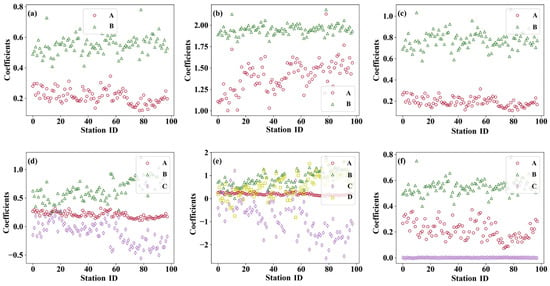
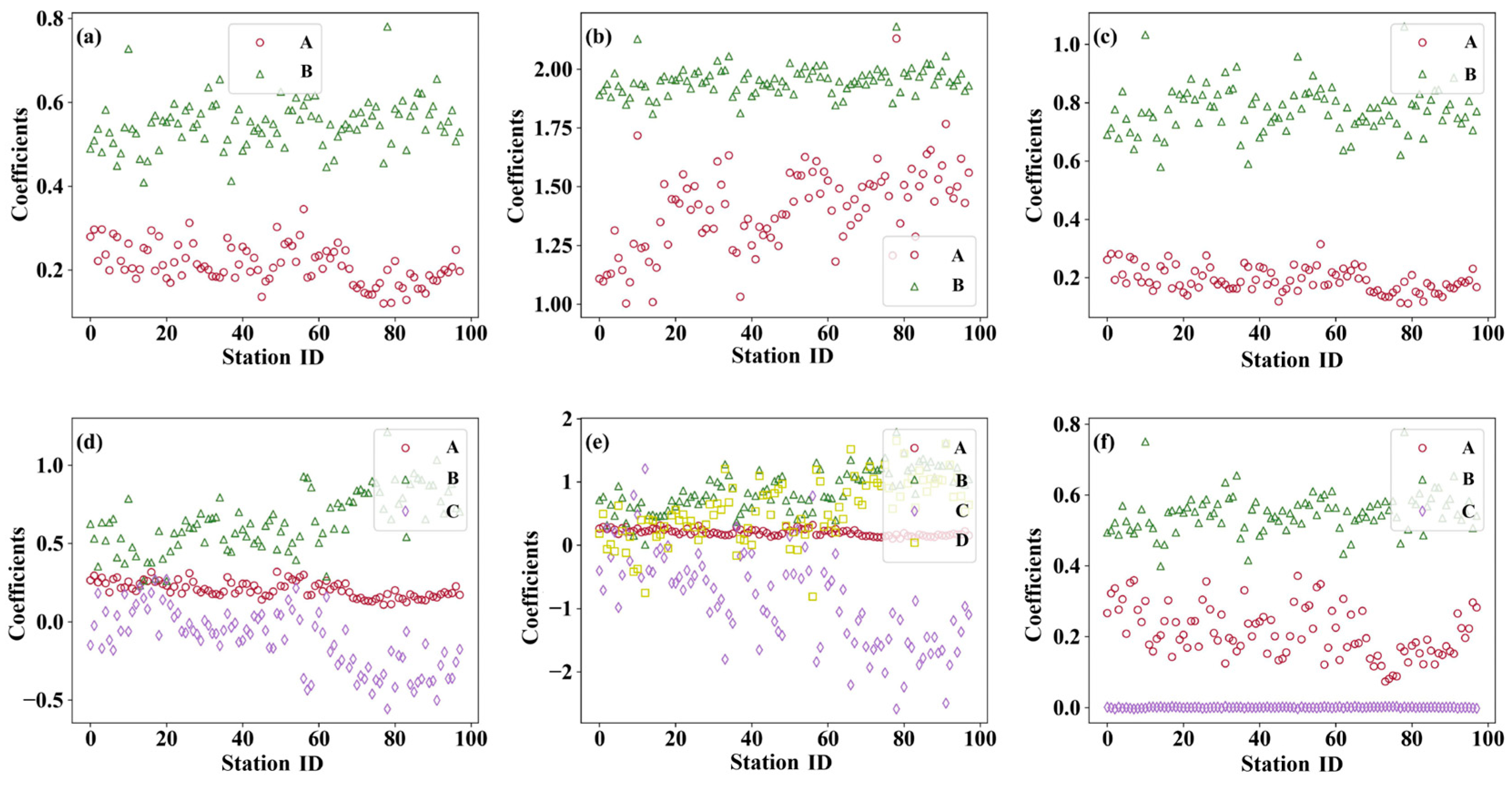
Figure 12 illustrates the fitted coefficients (A, B, C, and D) for six sunshine-based empirical models (M1–M6) across the 98 stations. Analysis revealed that the coefficients varied due to model structure and station-specific climatic factors. In models M4 and M5, coefficient A showed low sensitivity to station conditions, unlike in M1, M2, and M6. Conversely, coefficient C exhibited high variability across stations in all models except M6. For the Ångström–Prescott model (M1), the average coefficients were A = 0.21 (range: 0.12–0.35) and B = 0.55 (range: 0.41–0.78). For M5, the average coefficients we A = 0.20, B = 0.88, C = −0.86, and D = 0.56. Deviations from original model coefficients highlighted the need for local calibration to ensure accurate solar radiation estimation.

Figure 12. Fitted coefficients of the 6 sunshine-based empirical models at each of the 98 solar radiation stations. (a–f) correspond to M1 through M6, respectively.

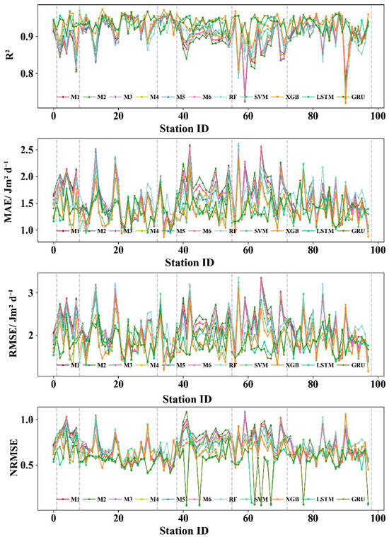
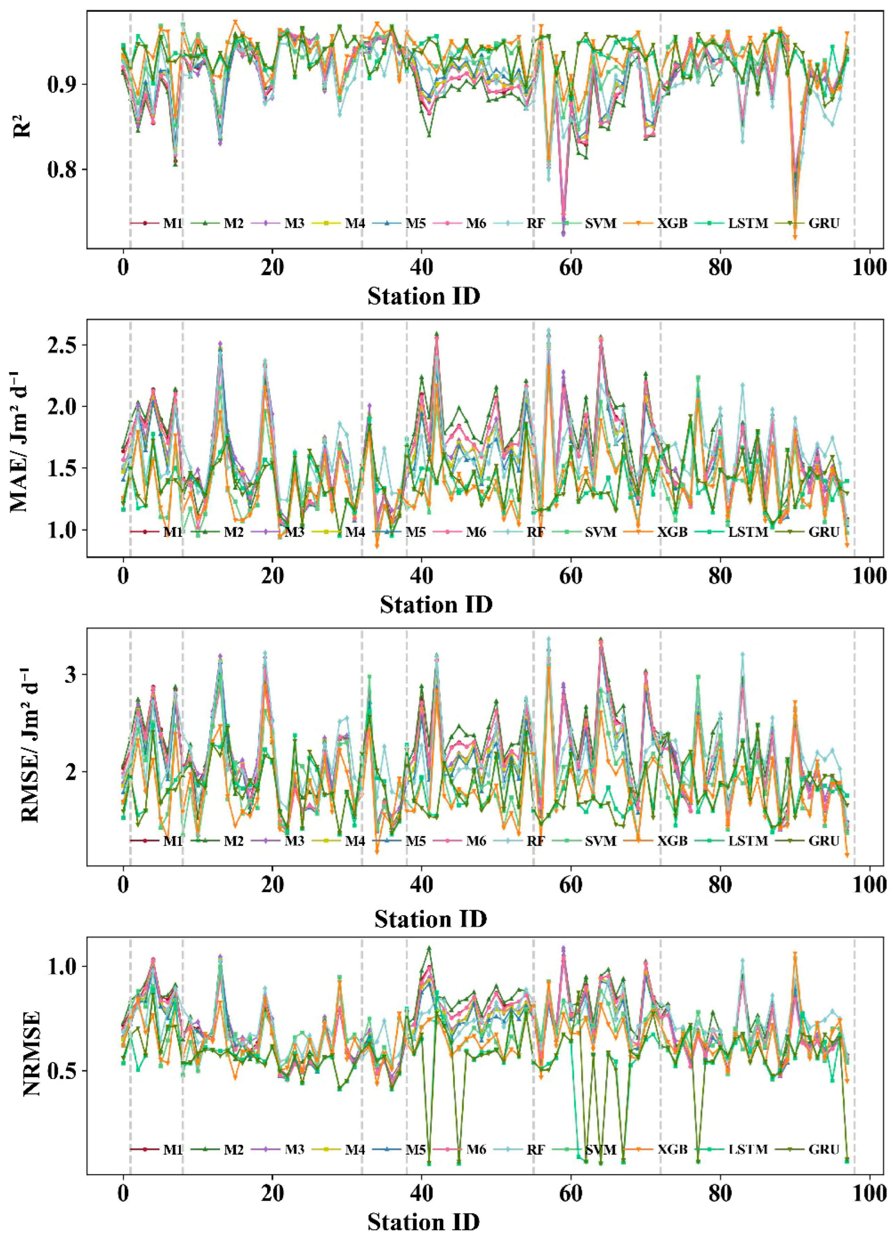
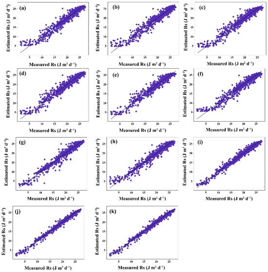
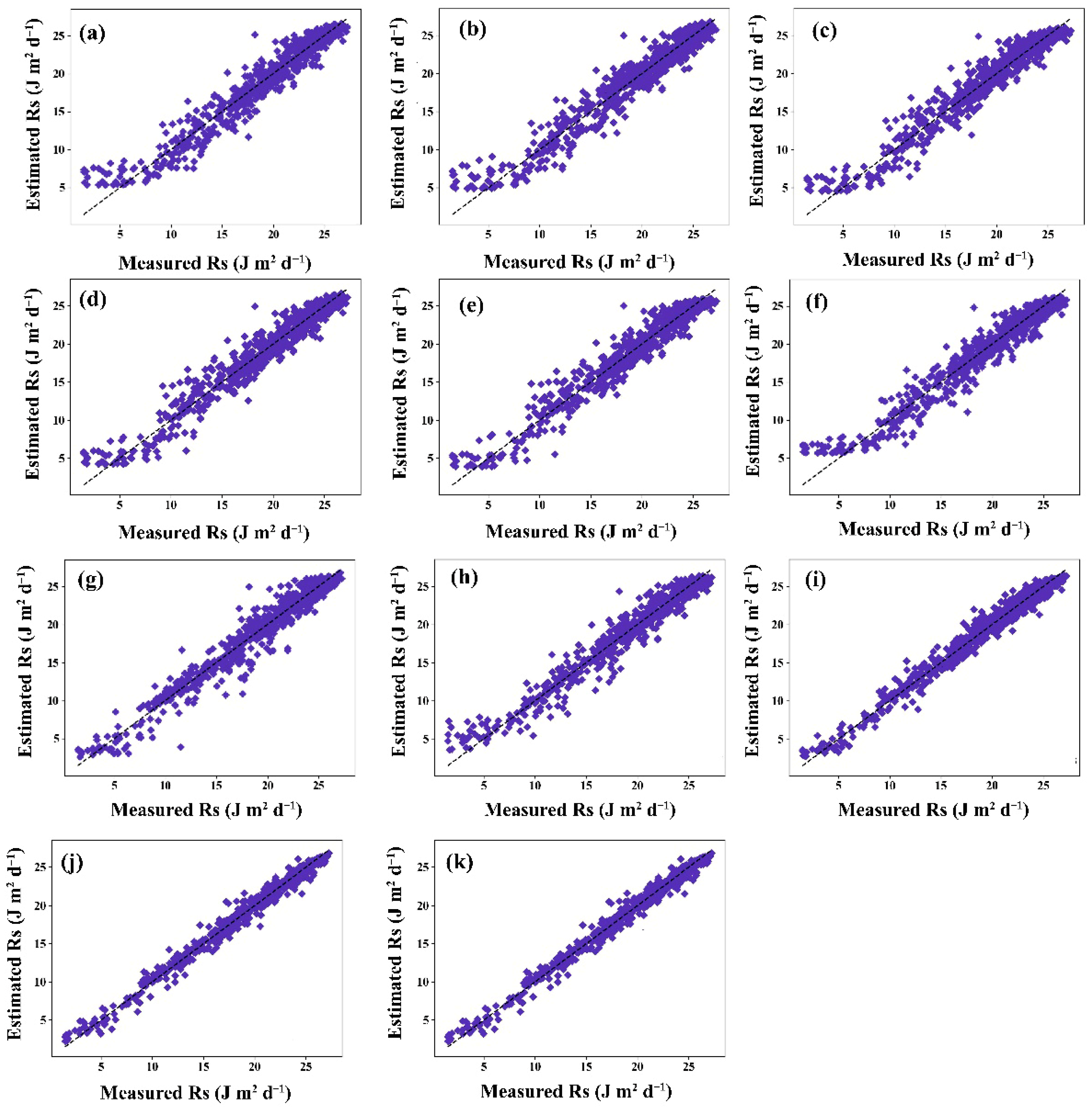
Figure 13 displays the MAE, RMSE, NRMSE, and R² values for the 11 models (six empirical, three machine learning, and two deep learning models) across 98 stations. The ML models (RF, SVM, and XGB) generally outperformed the empirical models (M1–M6) in RMSE and R² values, reflecting their ability to capture complex nonlinear relationships between inputs and outputs. However, in specific scenarios, the empirical models outperformed the machine learning models—particularly under simpler, stable, and low-noise conditions. The machine learning models excelled in noisy environments, such as regions with frequent cloud cover or dust, or areas with high spatiotemporal variability, owing to their robustness in modeling intricate dynamics. The DL models achieved the highest accuracy at all stations across all models. The scatterplots in Figure 14 further illustrate model performance, with the deep learning models showing closer alignment with observed values.

Figure 13. Values of statistical indicators for the 11 models at each of the 98 weather stations.

Figure 14. Scatterplots of the R_s values estimated by 6 selected empirical models, 3 ML models, and 2 DL models versus the corresponding observed values at 98 stations in China. (a–f) correspond to M1 through M6. (g) RF; (h) SVM; (i) XGB; (j) LSTM; (k) GRU. (Note: Dashed lines represent the 1:1 line).

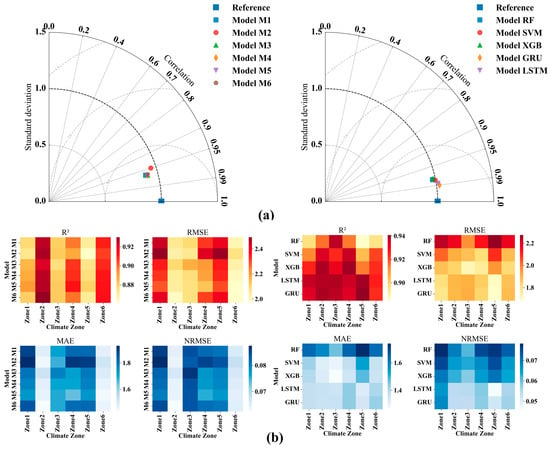
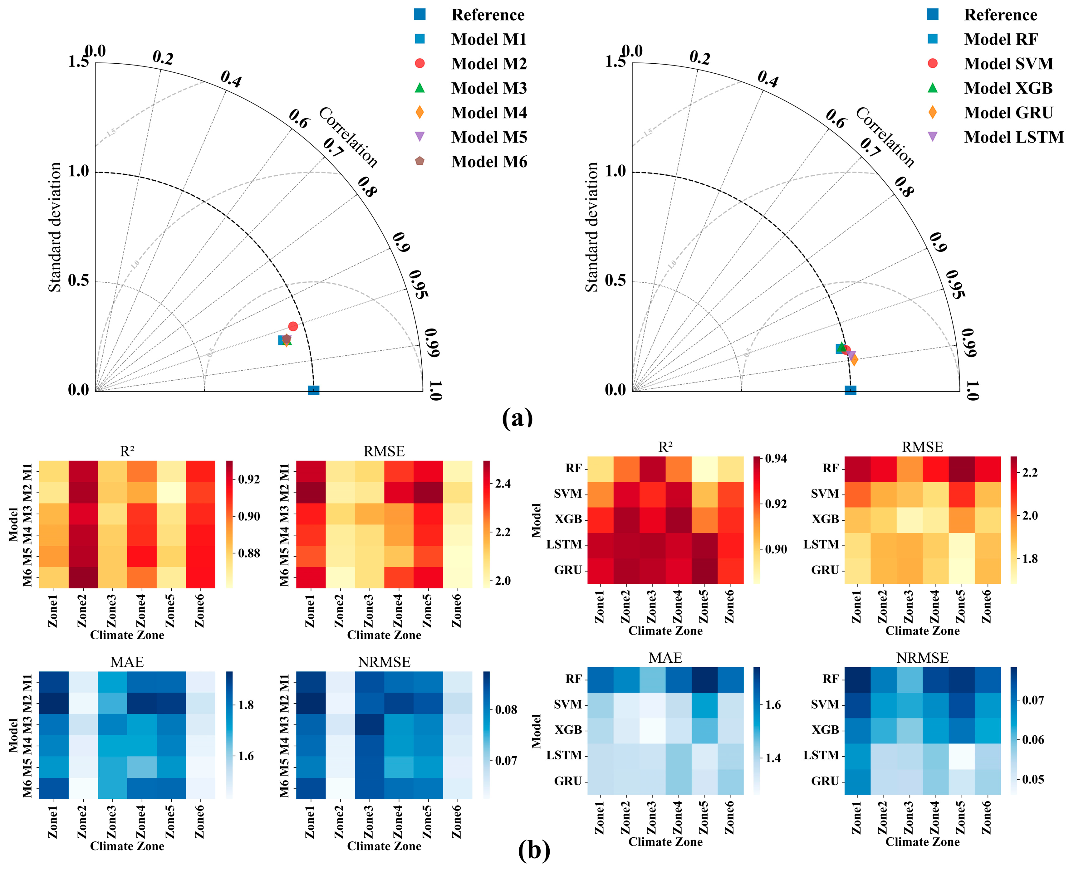
A Taylor diagram (Figure 15a) is employed to evaluate model performance by visualizing three metrics: correlation (angular divergence), standard deviation (radial distance), and centered root mean square error (distance from the reference point). Effective models demonstrate a high degree of correlation, minimal angular deviation, phase alignment, and proximity to the reference point—all of which indicate their ability to accurately capture the statistical properties of observed data. Poorly performing models show scattered points, larger angular deviations, and greater distances from the reference. Among the 11 models evaluated across the 98 stations, LSTM and GRU lay closest to the reference point, demonstrating superior predictive accuracy for solar radiation, whereas the empirical models showed greater deviations. Figure 15b displays the values of four statistical indicators (R², RMSE, MAE, and NRMSE) across the six radiation zones, confirming that the deep learning models (LSTM and GRU) consistently outperformed the others, although the empirical models showed competitive performance in Zone 2.

Figure 15. Taylor diagrams and error heat maps for the 11 models in solar radiation zones. (a) Taylor diagrams of ML and DL (right) and empirical models (left); (b) error heat maps of ML and DL (right) and empirical models (left).

To verify the statistical reliability of the modeling results, rigorous significance tests were conducted for the empirical models, as well as for the machine learning and deep learning frameworks. For the empirical models, the F-test was employed to examine the overall significance of the fitted regression equations, determining whether the model structure explained a significant proportion of the variance in solar radiation. Simultaneously, the t-test was applied to assess the statistical significance of individual regression coefficients, evaluating whether each predictor made a statistically significant contribution to the prediction. The test results clearly indicated that the F-statistics and t-statistics for the fitted formulas and coefficients at all selected stations achieved extreme significance (α = 0.01). This indicated that the established empirical models were statistically robust, and the inclusion of each explanatory variable was justified, laying a solid statistical foundation for the reliability of the model structure.

For the machine learning and deep learning models, paired t-tests were conducted on 10-fold cross-validation errors to statistically compare prediction performance among different models. The results confirmed that the performance differences between the optimal models and other comparative models were statistically significant (p < 0.05) in each solar radiation zone. Meanwhile, Shapiro–Wilk tests verified that the residuals followed an approximately normal distribution (p > 0.05), with a near-zero mean and no systematic bias. The F-tests further indicated significant differences between residual variance and original data variance (p < 0.01), and the coefficient of variation of cross-validation errors was below 0.08 for all models.

These statistical results rigorously confirmed that the performance differences observed in the comparative analysis were statistically significant rather than random fluctuations, ensuring the reliability of model comparisons and the rationality of the optimal model selection.

Table 5 presents a comprehensive comparison of training time and inference speed across different models, revealing a clear trade-off between model complexity and computational efficiency. The empirical models and traditional machine learning models (SVM, RF, and XGB) exhibited extremely fast training times, all within 0.3 s, with the empirical models taking less than 0.1 s and XGB achieving the shortest training time (0.05 s) among machine learning approaches. By contrast, the deep learning models (LSTM and GRU) required significantly longer training times, at 135.34 s and 165.25 s, respectively, due to their complex network structures and large parameter scales. Notably, despite the substantial gap in training efficiency, all models demonstrated comparable inference speeds, with inference times uniformly below 0.04 ms, indicating that once trained, even the deep learning models could meet the real-time prediction requirements of most application scenarios. This result highlighted that while deep learning models offer superior prediction accuracy, they incur higher training costs, whereas traditional models balance efficiency and performance, providing flexible options for different practical deployment needs.

Table 5. Training time and inference speed comparison of different models.

Model	Empirical Model	SVM	RF	XGBoost	LSTM	GRU
Training Time (s)	<0.1	0.019	0.29	0.05	135.34	165.25
Inference Speed (ms)	<0.01	0.039	0.04	0.01	0.028	0.039

Despite the satisfactory prediction performance achieved in this study, several important challenges remain for real-world and long-term applications. First, the deep learning models proposed are highly data-driven and rely on the statistical consistency between training and testing data. Under future climate change scenarios, significant data shifts may occur in solar radiation, temperature, cloud cover, and other meteorological variables, which could reduce model accuracy and generalizability. Further research is needed to develop climate-robust and domain-adaptive models that can maintain stable performance under nonstationary environmental conditions. Second, the high-performance deep learning architectures used in this study were relatively computationally intensive, which limits their direct deployment on resource-limited real-time edge devices for online forecasting. Future work will focus on model lightweighting, network compression, and efficient inference optimization to improve the feasibility of real-time edge deployment while maintaining high prediction accuracy.

4. Discussion

This study employed daily relative sunshine duration (S/S₀) from 819 meteorological stations to classify China into six solar radiation zones using k-means, hierarchical, and bisecting k-means clustering. Solar radiation data from 98 stations were used to develop six empirical models (M1–M6) and five machine learning/deep learning models (RF, SVM, XGB, LSTM, and GRU) for accurate solar radiation estimation.

4.1. Clustering Performance

K-means clustering outperformed hierarchical and bisecting k-means, achieving a Dunn index of 0.058 and a silhouette coefficient of 0.33, reflecting superior intra-cluster cohesion and inter-cluster separation. Its iterative optimization effectively captured spatial gradients in sunshine duration, balancing within-zone homogeneity and between-zone heterogeneity. This aligned with the findings of Li [41], who highlighted the efficacy of k-means clustering in climate zoning. Unlike Liu [5] and Qimeng [7], who identified five and nine zones, respectively, this study’s six-zone classification reflects methodological differences, emphasizing daily S/S₀ over monthly radiation or clearness indices. Existing zoning approaches, such as that of the European Commission [42], rely on simpler criteria such as monthly average radiation, adhering to the First Law of Geography. However, these methods lack precision and comparative analyses of clustering techniques. This study’s evaluation of multiple clustering methods and metrics addresses this gap, offering a robust framework for large-scale solar radiation zoning.

4.2. Empirical Model Adaptability

The empirical models showed regional variability in performance. M5 excelled in Zones 1, 3, 4, and 5, likely due to its exponential form capturing scattered radiation in humid and semi-humid climates (e.g., monsoonal regions). M6 performed best in arid Zones 2 and 6, aligning with direct radiation under clear skies. For the Ångström–Prescott model (M1), the average coefficients were a = 0.21 (range: 0.12–0.35) and b = 0.55 (range: 0.41–0.78). These values closely matched those reported by Fan [43] but deviated from the standard 0.25 and 0.50, indicating local calibration needs. M5’s coefficients were a = 0.20, b = 0.88, c = −0.86, and d = 0.56, which were similar to those reported by Fan [43] (a = 0.17, b = 0.92, c = −0.94, and d = 0.63). Variations from original coefficients underscored the necessity of local calibration for accurate solar radiation estimation.

4.3. Model Performance Comparison

The deep learning models (LSTM and GRU) significantly outperformed the machine learning (RF, SVM, and XGB) and empirical models, with LSTM achieving an R² value of 0.939, RMSE value of 1.702 MJ/m²/d, and MAE value of 1.319 MJ/m²/d. This aligned with the results by Xiaohui [44], who noted artificial neural networks’ strengths in modeling nonlinear climate data. GRU and XGB also showed strong performance, particularly in Zones 2 and 3, where clearer skies reduced variability. The empirical models performed better under simpler conditions (e.g., Zone 2), but their limitations in noisy or variable environments highlighted the superiority of deep learning models for complex datasets.

Benchmark comparisons demonstrated that the deep learning models (LSTM, GRU) consistently outperformed state-of-the-art machine learning models (XGB) across all six solar radiation zones in China, achieving higher R² and lower RMSE/MAE values, thus validating the necessity of adopting complex deep learning architectures for nationwide solar radiation estimation. This performance gap can be attributed to the inherent differences in model capabilities. Ensemble models such as XGB are highly efficient for tabular data and exhibit strong generalizability in small-to-medium datasets, but they are limited in capturing the long-term temporal dependencies and complex spatiotemporal nonlinear relationships in solar radiation time series. By contrast, deep learning models, especially LSTM, are designed to model sequential data and extract hierarchical spatiotemporal features, enabling them to better capture the dynamic variations of solar radiation driven by multiple meteorological factors across different climatic zones.

A critical review of existing solar radiation prediction research reveals a prominent gap: most studies conduct model evaluations at the national scale or for single regions, failing to systematically account for the significant regional heterogeneity in solar radiation driving factors and model adaptability across China’s diverse climatic and geographical zones. While many studies have applied machine learning and deep learning models for solar radiation estimation, few have conducted targeted, zone-specific comparative analyses to identify the most suitable models for different regional contexts, leading to suboptimal prediction accuracy in complex terrain and climate zones. This study directly addresses this gap by dividing China into distinct solar radiation zones, performing comprehensive multi-model comparisons within each zone, and developing a zoning-based prediction framework that tailors models to regional characteristics, thereby filling a critical void in the current literature and improving the reliability of nationwide solar radiation estimation.

4.4. Future Directions

The integrated zoning–prediction framework proposed in this study not only achieves high-accuracy solar radiation estimation for China but also exhibits strong extensibility to other application contexts, offering broad practical value in energy and environmental engineering. The core methodology, which combines quantitative clustering zoning, feature importance analysis, and data-driven model benchmarking, can be generalized to other data-driven tasks in the built environment, particularly heating, ventilation, and air conditioning fault detection and diagnosis using operational building data. To support this extensibility, two relevant dataset studies provide critical data foundations: ref. [45] introduced a semi-labeled dataset for fault detection in air handling units from a large-scale office, while ref. [46] presented real operational labeled data of air handling units from office, auditorium, and hospital buildings. The zoning-based approach proposed in this study can be adapted to these operational datasets to capture operational heterogeneity across different building types, identify building-specific fault patterns, and optimize the performance of fault detection and diagnosis models, thereby improving the robustness of heating, ventilation, and air conditioning system monitoring in real-world applications.

This study has several limitations that provide directions for future research. First, the framework is currently validated only within China; its generalizability to other regions with distinct geographical and climatic characteristics remains untested, which restricts broader applicability. Second, model performance may be sensitive to preprocessing choices (e.g., outlier removal and missing value imputation), as these steps were not systematically investigated in the current work. Finally, state-of-the-art deep learning architectures (such as attention-based or transformer-based models) were not included in the model benchmark. Future work should focus on: (1) extending the proposed zoning–prediction framework to other climatic and geographical regions worldwide to verify its cross-regional generalization ability; (2) systematically investigating the sensitivity of model performance to different data preprocessing strategies to enhance stability and reliability; and (3) incorporating state-of-the-art deep learning architectures (e.g., attention-based and transformer-based models) to further improve the accuracy and temporal–spatial modeling capacity of solar radiation estimation.

5. Conclusions

This study developed a nationwide zoning–prediction framework for solar radiation estimation across China.

(1)

Solar Radiation Zoning. Using daily relative sunshine duration from 819 meteorological stations, three clustering methods were compared, and results confirmed that k-means clustering achieved the best performance with the highest Dunn index (0.058) and silhouette index (0.33), indicating optimal intra-cluster homogeneity and inter-cluster separation. Accordingly, China was divided into six solar radiation zones that effectively reflect climatic and geographical heterogeneity and provide a solid spatial basis for regionalized prediction.

(2)

Key Influencing Factors. Correlation analysis and feature importance evaluation identified sunshine duration (S), extraterrestrial radiation (Ra), temperature difference (ΔT), and maximum temperature (Tmax) as the dominant meteorological variables affecting solar radiation, and significant regional heterogeneity in factor importance further verified the necessity of zoning.

(3)

Empirical Model Performance. Six sunshine-based empirical models exhibited clear regional adaptability, with Model 5 performing best in Zones 1, 3, 4, and 5, while Model 6 was optimal in Zones 2 and 6, and calibrated coefficients differed from standard values, highlighting the importance of local calibration for accurate estimation.

(4)

Machine Learning and Deep Learning Performance. Deep learning models significantly outperformed machine learning and empirical models: LSTM achieved the highest overall accuracy (R² = 0.939, RMSE = 1.702 MJ/m²/d, and MAE = 1.319 MJ/m²/d), followed closely by GRU, and among machine learning models, XGB performed best, followed by SVM and RF.

The proposed zoning–prediction framework effectively improves the accuracy of nationwide solar radiation estimation by accounting for regional heterogeneity, providing a reliable, systematic, and region-specific method for solar resource assessment, photovoltaic planning, and engineering applications across China.

Appendix A.1. K-Means Clustering

The core idea of k-means clustering is to iteratively optimize the grouping of data points so that those within each cluster are as close together as possible, while maximizing the distance between different clusters. Analysis of variance helps determine the optimal number of classifications by defining an F statistic, which is the ratio of the average between-group sum of squares to the average within-group sum of squares. A larger F value indicates a stronger relationship within groups and greater separation between them, making classification more reasonable. Factors in an experiment refer to variables that change, while levels denote their different states. The mathematical model is constructed as follows [47]:

$$\mathrm{F}=[{\mathrm{S}}_{\mathrm{S}\mathrm{A}}/(\mathrm{K}-1\left)\right][{\mathrm{S}}_{\mathrm{S}\mathrm{E}}/(\mathrm{n}-\mathrm{K}\left)\right]$$

(A1)

$${\mathrm{S}}_{\mathrm{S}\mathrm{A}}={\sum }_{\mathrm{i}=1}^{\mathrm{K}}{\mathrm{n}}_{\mathrm{i}}({\mathrm{x}}_{\mathrm{i}}-{\overline{\mathrm{x}}}_{\mathrm{i}}{)}^2$$

(A2)

$${\mathrm{S}}_{\mathrm{S}\mathrm{E}}={\sum }_{\mathrm{i}=1}^{\mathrm{K}}{\sum }_{\mathrm{j}=1}^{{\mathrm{n}}_{\mathrm{i}}}({\mathrm{x}}_{\mathrm{i}\mathrm{j}}-{\overline{\mathrm{x}}}_{\mathrm{i}}{)}^2$$

(A3)

where K is the number of levels; ${\mathrm{n}}_{\mathrm{i}}$ is the sample size under the i-th level; and ${\mathrm{S}}_{\mathrm{S}\mathrm{A}}$ and ${\mathrm{S}}_{\mathrm{S}\mathrm{E}}$ are the sum of squared deviations between groups and the sum of squared deviations within groups, respectively.

Appendix A.2. Hierarchical Clustering

Hierarchical clustering is an unsupervised learning method that divides a dataset into clusters by establishing hierarchical relationships among data points. The main idea is to create a tree-shaped dendrogram, either bottom–up or top–down, based on the similarity or distance between data points. The desired number of clusters can be achieved by setting a threshold or truncating the dendrogram. Each valid data object is treated as a variable in a matrix and positioned accordingly in rows and columns. Thus, n objects can be represented by p variables, forming an n × p data matrix [48]:

$$\left[\begin{array}{c}{\mathrm{x}}_{11}\cdots {\mathrm{x}}_{1\mathrm{f}}\cdots {\mathrm{x}}_{1\mathrm{p}}\\ \cdots \cdots \cdots \cdots \cdots \\ {\mathrm{x}}_{\mathrm{i}1}\cdots {\mathrm{x}}_{\mathrm{i}\mathrm{f}}\cdots {\mathrm{x}}_{\mathrm{i}\mathrm{p}}\\ \cdots \cdots \cdots \cdots \cdots \\ {\mathrm{x}}_{\mathrm{n}1}\cdots {\mathrm{x}}_{\mathrm{n}\mathrm{f}}\cdots {\mathrm{x}}_{\mathrm{n}\mathrm{p}}\end{array}\right]$$

(A4)

In this data matrix, different measurement units for each variable can lead to deviations in observed values. Therefore, an absolute value transformation is necessary to minimize the impact of these differences. Clustering plays a vital role in statistics, with group centroids, centers, and inter-group distances commonly used as clustering statistics. The choice of clustering statistic is critical; unreasonable selection may result in incorrect conclusions. For spatial clustering, Euclidean distance is typically employed as the clustering statistic.

For any two spatial points ${\mathrm{P}}_{\mathrm{i}}({\mathrm{x}}_{\mathrm{i}},{\mathrm{y}}_{\mathrm{i}}),{\mathrm{P}}_{\mathrm{j}}({\mathrm{x}}_{\mathrm{i}},{\mathrm{y}}_{\mathrm{i}}),{\mathrm{d}}_{\mathrm{i}\mathrm{j}}=\sqrt{({\mathrm{x}}_{\mathrm{i}}-{\mathrm{x}}_{\mathrm{j}}{)}^2+({\mathrm{y}}_{\mathrm{i}}-{\mathrm{y}}_{\mathrm{j}}{)}^2}$.

Clustering algorithms rely on a dissimilarity matrix, which transforms the data matrix to indicate the closeness of relationships between objects—reflecting their similarity or dissimilarity. This is represented as an n × n dimensional matrix:

$$\left[\begin{array}{ccccc}0& & & & \\ \mathrm{d}(2,1)& 0& & & \\ \mathrm{d}(2,1)& \mathrm{d}\left(2,1\right)0& & & \\ ⋮& ⋮& ⋮& & \\ \mathrm{d}(\mathrm{n},1)& \mathrm{d}(\mathrm{n},1)& \dots & \dots & 0\end{array}\right]$$

(A5)

As the similarity between objects i and j increases, the distance d (i, j) approaches 0. Thus, the dissimilarity matrix effectively represents the similarity among classified objects and serves as foundational data for clustering analysis. To ensure each variable contributes equally to the analysis, centralization and standardization transformations must be applied to the data.

Appendix A.3. Bisecting K-Means Clustering

The bisecting k-means clustering algorithm is a variant of the basic k-means algorithm, based on the following idea. To obtain K clusters, all datasets are initially treated as a single cluster V and placed in the cluster set S. Then, in a loop, one cluster is removed from S and the basic k-means algorithm is applied. By performing I iterations of bisection on the selected cluster, two clusters with the minimum total sum of squared errors (SSE) are identified and returned to set S. This process continues until K clusters are formed. Here, I denotes the number of bisection trials and SSE represents dispersion. Among multiple runs of the k-means algorithm, we select the clustering with the lowest SSE, indicating that its centroid best represents that cluster [49].

The SSE is defined as follows:

$$\mathrm{S}\mathrm{S}\mathrm{E}={\sum }_{\mathrm{i}=1}^{\mathrm{K}}{\sum }_{\mathrm{x}\in {\mathrm{c}}_{\mathrm{i}}}\mathrm{d}\mathrm{i}\mathrm{s}\mathrm{t}({\mathrm{c}}_{\mathrm{i}},\mathrm{x}{)}^2$$

(A6)

When bisecting, the k-means clustering algorithm is applied multiple times to achieve a minimum SSE, resulting in a local optimum rather than a global one. Consequently, the final centroid serves as the initial centroid for global optimization in the k-means algorithm. Unlike traditional k-means, this approach generates centroids through multiple bisections, thereby avoiding locally optimal results from randomly initialized centroids.

References

- Mrinal, R.; Ravi, S. A literature survey on load frequency control considering renewable energy integration in power system: Recent trends and future prospects. J. Energy Storage 2022, 45, 103717. [Google Scholar] [CrossRef] [Scilit]
- Sun, H.W.; Gui, D.W.; Yan, B.W. Assessing the potential of random forest method for estimating solar radiation using air pollution index. Energy Convers. Manag. 2016, 119, 121–129. [Google Scholar] [CrossRef] [Scilit]
- Zhou, Y.; Sha, X.; Wang, L. Spatial and temporal dynamics of solar energy resources in China and forecast of future solar radiation. J. Atmos. Sol.-Terr. Phys. 2025, 269, 106463. [Google Scholar] [CrossRef] [Scilit]
- Sanzana, T.; Tanvin, R.; Ul, A.I. Solar Energy in the United States: Development, Challenges and Future Prospects. Energies 2021, 14, 8142. [Google Scholar] [CrossRef] [Scilit]
- Liu, Y.; Zhou, Y.; Wang, D. Classification of solar radiation zones and general models for estimating the daily global solar radiation on horizontal surfaces in China. Energy Convers. Manag. 2017, 154, 168–179. [Google Scholar] [CrossRef] [Scilit]
- Hajou, A.; El, Y.M.; Yakoubi, H. Novel climate classification based on the information of solar radiation intensity: An application to the climatic zoning of Morocco. Energy Convers. Manag. 2021, 247, 114770. [Google Scholar] [CrossRef] [Scilit]
- Qimeng, C.; Yan, L.; Kailin, L. Solar radiation zoning and daily global radiation models for regions with only surface meteorological measurements in China. Energy Convers. Manag. 2020, 225, 113447. [Google Scholar] [CrossRef] [Scilit]
- Fan, J.; Chen, B.; Wu, L. Evaluation and development of temperature-based empirical models for estimating daily global solar radiation in humid regions. Energy 2018, 144, 903–914. [Google Scholar] [CrossRef] [Scilit]
- Liu, Z.H.; Qiu, R.J.; Liu, C.W. Determination of generalized solar radiation model based on sunshine percentage for improving reference crop evapotranspiration estimation accuracy. Water Sav. Irrig. 2023, 2, 80–88. [Google Scholar]
- Almorox, J.; Bocco, M.; Willington, E. Estimation of daily global solar radiation from measured temperatures at Cañada de Luque, Córdoba, Argentina. Renew. Energy 2013, 60, 382–387. [Google Scholar] [CrossRef] [Scilit]
- Fan, J.; Wang, X.; Wu, L. New combined models for estimating daily global solar radiation based on sunshine duration in humid regions: A case study in South China. Energy Convers. Manag. 2018, 156, 618–625. [Google Scholar] [CrossRef] [Scilit]
- Oyewola, O.M.; Patchali, T.E.; Ajide, O.O. Global solar radiation predictions in Fiji Islands based on empirical models. Alex. Eng. J. 2022, 61, 8555–8571. [Google Scholar] [CrossRef] [Scilit]
- Tercha, W.; Tadjer, A.S.; Chekired, F. Machine Learning-Based Forecasting of Temperature and Solar Irradiance for Photovoltaic Systems. Energies 2024, 17, 1124. [Google Scholar] [CrossRef] [Scilit]
- Venkatesh, B.; Shekeew, A.I.M.; Ma, J. Feasibility-guaranteed machine learning unit commitment: Fuzzy Optimization approaches. Appl. Energy 2025, 379, 124923. [Google Scholar] [CrossRef] [Scilit]
- Barancsuk, L.; Groma, V.; Kocziha, B. Hybrid ultra-short term solar irradiation forecasting using resource-efficient multi-step long-short term memory. Renew. Energy 2025, 247, 122962. [Google Scholar] [CrossRef] [Scilit]
- Narjes, A.; Maryam, Y.; Meisam, F. Deep learning based long-term global solar irradiance and temperature forecasting using time series with multi-step multivariate output. Renew. Energy 2023, 206, 135–147. [Google Scholar]
- Allen, R.G.; Pereira, L.S.; Raes, D.; Smith, M. Crop Evapotranspiration—Guidelines for Computing Crop Water Requirements—FAO Irrigation and Drainage Paper 56; Food and Agriculture Organization of United Nations: Rome, Italy, 1998. [Google Scholar]
- Kirmani, S.; Jamil, M.; Rizwan, M. Empirical correlation of estimating global solar radiation using meteorological parameters. Int. J. Sustain. Energy 2015, 34, 327–339. [Google Scholar] [CrossRef] [Scilit]
- Ångström, A. Solar and terrestrial radiation. Quart. J. Roy Met. Soc. 1924, 50, 121–125. [Google Scholar]
- Prescott, J.A. Evaporation from water surface in relation to solar radiation. Trans. Roy Soc. Sci. Aust. 1940, 64, 114–125. [Google Scholar]
- Bakirci, K. Correlations for estimation of daily global solar radiation with hours of bright sunshine in Turkey. Energy 2009, 34, 485–501. [Google Scholar] [CrossRef] [Scilit]
- Toğrul, I.T.; Toğrul, H.; Evin, D. Estimation of global solar radiation under clear sky radiation in Turkey. Renew. Energy 2000, 21, 271–287. [Google Scholar] [CrossRef] [Scilit]
- Ögelman, H.; Ecevit, A.; Tasdemiroğlu, E. A new method for estimating solar radiation from bright sunshine data. Sol. Energy 1984, 33, 619–625. [Google Scholar] [CrossRef] [Scilit]
- Bahel, V.; Bakhsh, H.; Srinivasan, R. A correlation for estimation of global solar radiation. Energy 1987, 12, 131–135. [Google Scholar] [CrossRef] [Scilit]
- Toğrul, I.T.; Onat, E. A study for estimating solar radiation in Elaziğ using geographical and meteorological data. Energy Convers. Manag. 1999, 40, 1577–1584. [Google Scholar] [CrossRef] [Scilit]
- Eshetu, D.K.; Seifu, K.T.; Alamirew, T. Estimating reservoir evaporation rate: Fusing remotely sensed solar radiation and temperature features with machine learning algorithms. Theor. Appl. Climatol. 2025, 156, 175. [Google Scholar] [CrossRef] [Scilit]
- Bell, B.; Neudecker, D.; Grosskopf, M. Identifying nuclear data correlated through predicting bias in integral experiments via applying principal component analysis to random forest. Stat. Anal. Data Min. 2025, 18, e70014. [Google Scholar] [CrossRef] [Scilit]
- Breiman, L. Random forests. Mach. Learn. 2001, 45, 5–32. [Google Scholar] [CrossRef] [Scilit]
- Basha, S.S.; Rao, N.A. Optimizing solar radiation prediction: A novel SVM approach for renewable energy systems. Int. J. Inf. Technol. 2025, 17, 1–13. [Google Scholar] [CrossRef] [Scilit]
- Vapnik, V.N. The Nature of Statistical Learning Theory; Springer Science & Business Media: Berlin/Heidelberg, Germany, 2013. [Google Scholar]
- Xu, S.; Wu, H.; Chen, J.; Jia, H. The application of support vector machine (SVM) in industrial carbon accounting prediction and green electricity control strategies. E3S Web Conf. 2025, 615, 01012. [Google Scholar] [CrossRef] [Scilit]
- Maitreyee, T.; Jagadeesh, A.; Turuganti, V. Support vector machine (SVM) model development for prediction of fecal coliform of Upper Green River Watershed, Kentucky, USA. Sustain. Water Resour. Manag. 2024, 10, 114. [Google Scholar] [CrossRef] [Scilit]
- Cheenkachorn, K.; Prapainainar, C.; Wijakmatee, T. Machine learning-driven modeling of biomass pyrolysis product distribution through thermal parameter sensitivity. Renew. Energy 2025, 248, 123108. [Google Scholar] [CrossRef] [Scilit]
- Deo, C.R.; Samui, P.; Kim, D. Estimation of monthly evaporative loss using relevance vector machine, extreme learning machine and multivariate adaptive regression spline models. Stoch. Environ. Res. Risk Assess. 2016, 30, 1769–1784. [Google Scholar] [CrossRef] [Scilit]
- Zhang, X.; Wang, Y.; Zhuang, Z. Comparison of simulating visibility using XGBoost and IMPROVE method: A case study in East China. Front. Environ. Sci. 2025, 12, 1534113. [Google Scholar] [CrossRef] [Scilit]
- Özdemir, R.; Taşyürek, M.; Aslantaş, V. Improved marine predators algorithm and extreme gradient boosting (XGBoost) for shipment status time prediction. Knowl.-Based Syst. 2024, 294, 111775. [Google Scholar] [CrossRef] [Scilit]
- Irshad, K.; Islam, N.; Gari, A.; Algarni, S.; Alqahtani, T.; Imteyaz, B. Arithmetic optimization with hybrid deep learning algorithm based solar radiation prediction model. Sustain. Energy Technol. Assess. 2023, 57, 103165. [Google Scholar] [CrossRef] [Scilit]
- Hochreiter, S.; Schmidhuber, J. Long Short-Term Memory. Neural Comput. 1997, 9, 1735–1780. [Google Scholar] [CrossRef] [Scilit]
- Mehdi, J.; Masoud, K.; Mumtaz, A. A novel global solar exposure forecasting model based on air temperature: Designing a new multi-processing ensemble deep learning paradigm. Expert Syst. Appl. 2023, 222, 119811. [Google Scholar] [CrossRef] [Scilit]
- Gupta, R.; Yadav, K.A.; Jha, K.S. Harnessing the power of hybrid deep learning algorithm for the estimation of global horizontal irradiance. Sci. Total Environ. 2024, 943, 173958. [Google Scholar] [CrossRef] [Scilit]
- Li, M.F. General models for estimating daily global solar radiation for different solar radiation zones in mainland China. Energy Convers. Manag. 2013, 70, 139–148. [Google Scholar] [CrossRef] [Scilit]
- Palz, W.; Greif, J. European Solar Radiation Atlas: Solar Radiation on Horizontal and Inclined Surfaces; Springer: Berlin/Heidelberg, Germany, 1996. [Google Scholar]
- Fan, J.; Wu, L.; Zhang, F. Evaluation and development of empirical models for estimating daily and monthly mean daily diffuse horizontal solar radiation for different climatic regions of China. Renew. Sustain. Energy Rev. 2019, 105, 168–186. [Google Scholar] [CrossRef] [Scilit]
- Yan, X.; Yang, N.; Ao, R.; Mohammadian, A.; Liu, J.; Cao, H.; Yin, P. Deep learning for daily potential evapotranspiration using a HS-LSTM approach. Atmos. Res. 2023, 292, 106856. [Google Scholar] [CrossRef] [Scilit]
- Wang, S.; Eum, I.; Park, S.; Kim, J. A semi-labelled dataset for fault detection in air handling units from a large-scale office. Data Brief 2024, 57, 110956. [Google Scholar] [CrossRef] [Scilit]
- Wang, S. Real operational labeled data of air handling units from office, auditorium, and hospital buildings. Sci. Data 2025, 12, 1481. [Google Scholar] [CrossRef] [Scilit]
- Muhammad, R.A.; Singh, K.P.; Salim, H. Suspended Sediment Modeling Using a Heuristic Regression Method Hybridized with Kmeans Clustering. Sustainability 2021, 13, 4648. [Google Scholar] [CrossRef] [Scilit]
- Riyahi, M.; Martín, G.A. Optimizing capacity expansion modeling with a novel hierarchical clustering and systematic elbow method: A case study on power and storage units in Spain. Energy 2025, 323, 135788. [Google Scholar] [CrossRef] [Scilit]
- Zhao, C.; Li, X.; Cang, Y. Bisecting k -means clustering based face recognition using block-based bag of words model. Optik Int. J. Light Electron Opt. 2015, 126, 1761–1766. [Google Scholar] [CrossRef] [Scilit]
Disclaimer/Publisher’s Note: The statements, opinions and data contained in all publications are solely those of the individual author(s) and contributor(s) and not of MDPI and/or the editor(s). MDPI and/or the editor(s) disclaim responsibility for any injury to people or property resulting from any ideas, methods, instructions or products referred to in the content. |
© 2026 by the authors. Licensee MDPI, Basel, Switzerland. This article is an open access article distributed under the terms and conditions of the Creative Commons Attribution (CC BY) license.