Physics-Driven Hybrid Framework for Vehicle State Estimation Using Residual Learning and Adaptive UKF

Abstract

Accurate estimation of vehicle sideslip angle and lateral velocity is essential for the stability control of Advanced Driver Assistance Systems (ADASs). Traditional physics-based observers often exhibit dynamic response distortions under stability-limit conditions due to unmodeled tire relaxation effects, while data-driven methods lack physical interpretability. This paper proposes a Physics-Driven Hybrid Estimation Framework (PD-HEF) to bridge this gap. First, a nonlinear nominal model is constructed as a physical skeleton, and dynamic residual equations are derived to define learning targets. Second, a Spatio-Temporal Feature Coupled Residual Network is designed to capture time-domain phase lag and compensate for spatial nonlinear deviations. Furthermore, a hybrid unscented Kalman filter is developed to inject predicted residuals into the sigma-point evolution. A Dual-Layer Adaptive Mechanism is also introduced to regulate trust weights based on innovation statistics. Joint simulations demonstrate that the proposed framework reduces the root mean square error by over 60% compared to traditional observers while satisfying real-time constraints.

1. Introduction

As the automotive industry accelerates its evolution towards CASE (Connected, Autonomous, Shared, Electric), various active safety systems (such as Electronic Stability Control, ESC) and high-level autonomous driving functions (such as Model Predictive Control for trajectory tracking) have placed unprecedented demands on the perception accuracy of vehicle chassis dynamic states [1,2,3]. Among numerous state variables, the vehicle sideslip angle ($\beta$) and lateral velocity ($v_y$) directly determine the lateral stability boundaries and handling limits of the vehicle. However, due to cost constraints in mass-produced passenger vehicles, high-precision optical sensors or dual-antenna differential GNSS/INS systems capable of directly measuring these states are difficult to deploy on a large scale [4,5]. Existing onboard sensors primarily provide information such as wheel speed, yaw rate, and acceleration [6]. Furthermore, these sensors are susceptible to noise pollution and zero-point drift in harsh operating environments [7,8]. Therefore, achieving high-precision, robust Virtual Sensing via observer technology based on low-cost onboard sensors has become a core challenge in the field of intelligent vehicle dynamics control.

1.1. Related Work and Limitations Analysis

Existing vehicle state estimation methods can be categorized into Model-based Approaches and Data-driven Approaches.

Model-based Approaches and Inadequacy of Physical Models under Transient Conditions. These methods utilize Newton–Euler equations to construct a state space and perform state recursive inference via Extended Kalman Filter (EKF), unscented Kalman filter (UKF), or Sliding Mode Observer (SMO) [9,10]. Their performance ceiling strictly depends on the fidelity of the dynamic model, with the accuracy of the tire model being particularly critical. Current mainstream research mostly employs the classic Pacejka magic formula or the Dugoff model [11,12]. Although these models perform excellently under steady-state conditions, they are essentially empirical fits based on bench tests, which imply the assumption that lateral force generation is instantaneous with respect to the slip angle input. However, under high-dynamic conditions such as high-speed double lane change (DLC), the viscoelasticity of tire rubber material causes the deformation of the contact patch to lag behind the rim motion, creating a significant relaxation length effect [13,14]. This physical characteristic leads to a first-order lag in the generation of lateral force in the time domain, causing phase-lead errors in traditional observers. Additionally, commonly used single-track models typically ignore vertical load transfer caused by body roll. According to Jensen’s Inequality, under high lateral acceleration limits, load transfer results in a reduction in the total available lateral tire force, leading the nominal model to overestimate the vehicle’s stability limit [15,16].

Data-Driven Approaches and Black Box Interpretability Issues. To overcome the complexity of analytical modeling, methods based on deep learning have emerged in recent years. Using Recurrent Neural Networks (RNNs), Long Short-Term Memory networks (LSTMs), or Convolutional Neural Networks (CNNs) to directly establish nonlinear mappings between sensor data and vehicle states has demonstrated powerful fitting capabilities [17,18,19]. However, pure data-driven methods often operate as black boxes lacking clear physical interpretability. Their prediction accuracy is highly dependent on the coverage of the training data, leading to extremely poor extrapolation capabilities in out-of-distribution (OOD) scenarios [20,21]. For instance, when a vehicle enters a low-adhesion icy road not included in the training set, a pure neural network is prone to outputting estimation results that violate physical conservation laws, presenting an unacceptable risk to the safety of autonomous driving systems.

The Fusion Gap in Hybrid Physics: Data-Driven and System Uncertainty. Given the above limitations, Physics-Guided Machine Learning (PGML) has emerged to bridge analytical and purely data-driven methods [22,23]. Beyond standard Gaussian observers, guaranteeing dynamic safety in Advanced Driver Assistance Systems (ADASs) requires bounding estimation uncertainties.

However, regarding the internal structural fusion of neural networks and vehicle kinematics, existing hybrid chassis observers primarily rely on ‘post-estimation weighted averaging’ or use physical equations merely as soft loss-function penalties. These approaches fail to fundamentally reconcile the internal evolution errors within the state differential equations, risking physical violations during out-of-distribution (OOD) extrapolation limits [24,25].

Furthermore, regarding system safety and control feasibility, traditional point-based estimation frameworks natively fail to formulate an indicator representing the estimation uncertainty envelope. If the bounds associated with unmodeled dynamics are not rigorously quantified, downstream autonomous control frameworks (e.g., Model Predictive Control tracking) may suffer from critical instability. To comprehensively limit tracking deviations under bounded disturbances, robust Linear Matrix Inequality (LMI) and $H_{\infty }$ optimal techniques have established profound baselines. Simultaneously, to suit advanced interconnected environments, integrating robust chassis observers explicitly with event-triggered-based IoT architectures has proven effective in minimizing communication burdens while preserving dynamic stability [26]. More recently, overcoming pure probabilistic limitations, set-membership techniques have pioneered deterministic uncertainty evaluations. Groundbreaking methodologies including Zonotopic Kalman Filters [27] and Interval Observers coupled with Extended Kalman Filters [28] have successfully constructed strict mathematical bounds guaranteeing that the vehicle sideslip angle strictly resides within a precise, computable envelope despite profound measurement and modeling uncertainties. Inspired by the rigorous safety philosophy of these envelope-bounding frameworks, our proposed PD-HEF fundamentally aims to compress this underlying mechanistic deviation.

1.2. Main Research Content

This paper proposes a high-precision collaborative estimation method (PD-HEF). The core novelty is grounded in a Dynamic Residual Target Learning strategy. Unlike traditional hybrid methods that attempt to map full vehicle states via networks, our PD-HEF structurally isolates the precise physical discrepancy (i.e., extracting the unmodeled time-domain differential phase-lag and spatial load transfer effects). The neural network is highly constrained to learn only this explicit differential residual (${\dot{x}}_{true}-f_{nom}$), which is then deeply embedded into the numerical integration level of the physical skeleton. This hybrid configuration guarantees critical physical conservation laws while utilizing data-driven agility to counteract limit-handling transient failures.

Furthermore, addressing the selection of the foundational physical skeleton, it is acknowledged that high-fidelity multibody models can nowadays be executed in real time on powerful research computing platforms. However, the engineering target of this study firmly roots in mass-produced, cost-sensitive vehicle platforms. Dedicated in-vehicle microcontrollers (such as standard Automotive Safety Integrity Level (ASIL) Domain Control Units) possess highly restricted floating-point matrix processing capabilities. Propagating the highly coupled Jacobian mechanisms of multibody models at high operational frequencies (e.g., 100 Hz) often exceeds allowable latency budgets. Consequently, the proposed PD-HEF is purposefully designed to extract the lightweight computational footprint of a 3-DOF single-track model, while relying on the offline-trained ST-ResNet to implicitly recover the complex limit-handling dynamics, achieving a pragmatic bridge between theoretical accuracy and mass-production hardware limits.The main innovations are as follows:

(1) Construction of a Dynamic Compensation Mechanism based on ST-ResNet: Addressing the phase-lag issue caused by the traditional magic formula ignoring the relaxation length effect, a residual network containing LSTM units is designed. This network takes the prediction error of the nominal physical model as guidance, specifically capturing the time-domain lag characteristics in tire transient response and spatial nonlinear deviations caused by load transfer, providing a high-precision differential patch for the physical skeleton.

(2) Proposal of a Hybrid-UKF Closed-Loop Estimation Architecture with Embedded Neural Network Compensation: A hybrid sigma-point evolution operator is derived to directly inject the dynamic residual terms predicted by ST-ResNet into the time update step of the unscented Kalman filter. This architecture retains the deterministic constraints of physical equations on state evolution (basic trend) while correcting the model’s trajectory at limit edges using data-driven means (high-order correction), effectively solving the failure problem of traditional filters in strongly nonlinear regions.

(3) Design of a Dual-Layer Adaptive Mechanism (DLAM) based on Fuzzy Logic and Innovation Statistics: The bottom layer utilizes real-time statistical characteristics of the innovation sequence to adaptively adjust the measurement noise covariance, resisting sensor environmental interference. The top layer constructs a fuzzy logic scheduler to dynamically regulate the trust weights between the physical model and the neural network, as well as the process noise, based on the rate of vehicle lateral acceleration deviation and yaw rate gradient. This mechanism realizes a soft switching of the system—relying on physical laws in the steady-state region and data compensation in the limit region—achieving optimal estimation performance under all working conditions.

2. Vehicle Dynamics Modeling and Residual Definition

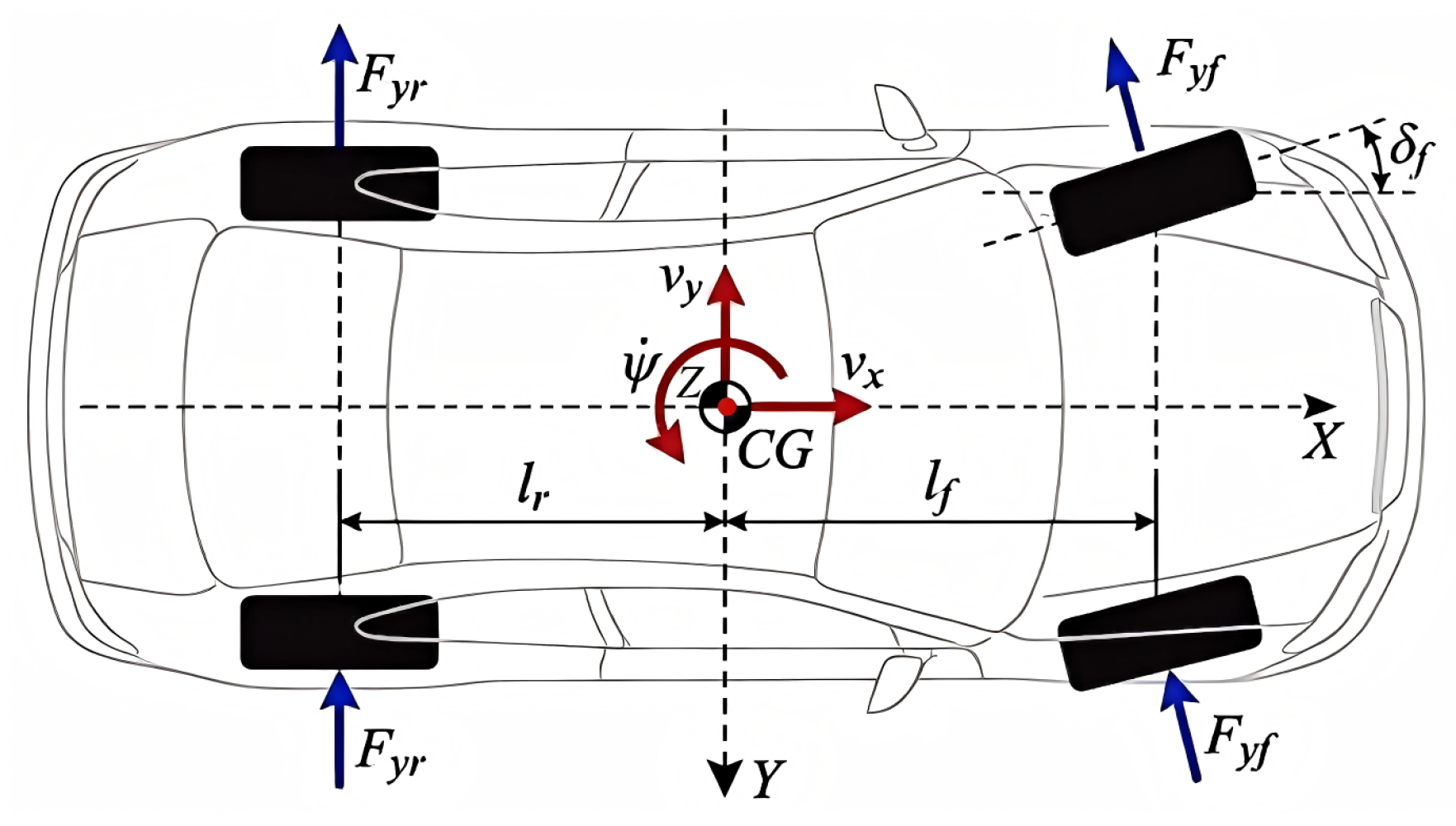
In the PD-HEF, to ensure the real-time performance of state inference and provide deterministic physical constraints, this paper constructs a 3-DOF vehicle model as the skeleton of the physics-driven layer, referred to as the nominal model (Figure 1).

Assuming the vehicle travels on a horizontal road surface and ignoring the high-frequency dynamics of suspension roll and pitch, the nominal state evolution equations are established based on Newtonian mechanics (referenced from classic vehicle dynamics frameworks [29]). Furthermore, the spatial definitions mapped in Figure 1 strictly verify compliance with standard ISO 8855 [30] coordinate system conventions, wherein the X-axis continuously signifies forward longitudinal motion, the Y-axis determines corresponding lateral kinematics, and the Z-axis extends vertically upwards governing the specific yaw rate.

The state vector of the system is defined as $\mathbf{x}={[v_x,v_y,\dot{\psi }]}^T$, and the control input vector is $\mathbf{u}={[{\delta }_f,a_{x,m}]}^T$, controlling longitudinal, lateral, and yaw motions.

Assuming the vehicle travels on a horizontal road surface and ignoring the high-frequency dynamics of suspension roll and pitch, the nominal state evolution equations are established based on Newton–Euler equations: ${\mathbf{f}}_{nom}(\mathbf{x},\mathbf{u})$.

$$\left[\begin{array}{c}{\dot{v}}_x\\ {\dot{v}}_y\\ \ddot{\psi }\end{array}\right]=\left[\begin{array}{c}{a}_{x,m}+v_y\dot{\psi }\\ {\displaystyle \frac{1}{m}}\left(F_{yf}cos{\delta }_f+F_{yr}\right)-v_x\dot{\psi }\\ {\displaystyle \frac{1}{I_z}}\left(l_f{F}_{yf}cos{\delta }_f-l_r{F}_{yr}\right)\end{array}\right]$$

(1)

where $v_x$ is the longitudinal velocity at the CG; $v_y$ is the lateral velocity at the CG; $\dot{\psi }$ is the yaw rate; m is the total vehicle mass; $I_z$ is the moment of inertia around the Z-axis; $l_f$ and $l_r$ are the horizontal distances from the CG to the front and rear axles; ${\delta }_f$ is the front-wheel steering angle input; $a_{x,m}$ is the measured longitudinal acceleration (used here to decouple longitudinal dynamics and reduce interference); $F_{yf}$ and $F_{yr}$ are the front- and rear-tire lateral forces.

Operating heavily under mass-production cost-containment constraints, the algorithm intrinsically presumes the vehicle exclusively integrates commercial, low-cost chassis sensory configurations (a standard ESP-grade inertial maneuvering unit (IMU) alongside a conventional column steering angle sensor (SAS)). Driven by this explicit hardware topology layout, the measurement vector fed into the online observer is defined as $\mathbf{z}={[a_{x,m},a_{y,m},\dot{\psi },{\delta }_f]}^T$. Meanwhile, overcoming the physical unavailability of precision optical velocity instrumentation, the deeply implicit target variables targeted universally for algorithmic estimation encompass the lateral velocity ($v_y$) coupled structurally with the overall mass center sideslip angle ($\beta$).

In the nominal model, assuming tires are in a steady linear or weakly nonlinear region, the relationship between the lateral tire force $F_y$ and the tire slip angle $\alpha$ is constructed using the simplified Pacejka magic formula [31].

$$F_{y,i}=\mu Dsin\left(Carctan\left(B{\alpha }_i-E\left(B{\alpha }_i-arctan\left(B{\alpha }_i\right)\right)\right)\right)$$

(2)

where $\mu$ is the friction coefficient, and B, C, D, E are stiffness, shape, peak, and curvature factors, respectively. Tire sideslip angles ${\alpha }_i$ are derived from kinematic geometry:

$$\begin{array}{cc}\hfill {\alpha }_f& ={\delta }_f-arctan\left({\displaystyle \frac{v_y+l_f\dot{\psi }}{v_x}}\right)\hfill \end{array}$$

(3)

$$\begin{array}{cc}\hfill {\alpha }_r& =-arctan\left({\displaystyle \frac{v_y-l_r\dot{\psi }}{v_x}}\right)\hfill \end{array}$$

(4)

2.1. Deviation in Dynamic Limit-Handling Conditions

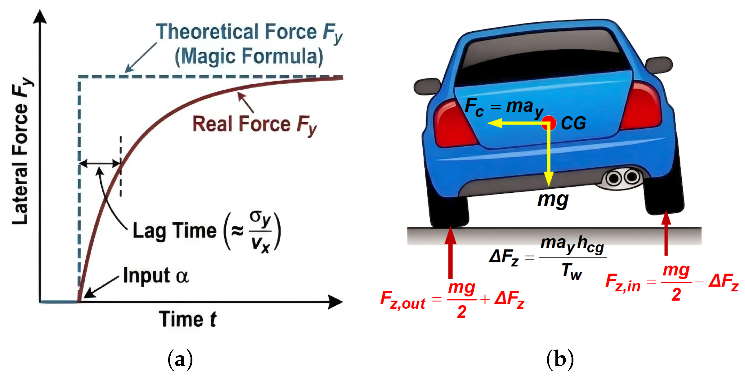
Under limit-handling conditions like high-speed double lane changes, significant dynamic deviations exist between the real vehicle system and the nominal model. These deviations are not random noise but possess strong physical laws and structural biases, primarily stemming from two core physical sources (Figure 2).

2.1.1. Time-Domain Feature: Phase Lag Induced by Tire Relaxation Effect

As shown in Figure 2a, the nominal model assumes lateral force is established synchronously with sideslip angle ($Fy\propto \alpha$). However, the viscoelasticity of real tire rubber causes the tire contact patch deformation to lag, characterized by relaxation length (${\sigma }_y$). The real lateral force response follows a first-order delay.

$${\displaystyle \frac{{\sigma }_y}{v_x}}{\dot{F}}_y^{true}+F_y^{true}=F_y^{ss}\left(\alpha \right)$$

(5)

where $F_y^{true}$ and $F_y^{ss}$ represent the actual lateral force and steady-state lateral force, respectively. Ignoring the ${\dot{F}}_y^{true}$ term under high-frequency steering inputs leads the nominal model to calculate a lateral force response that leads the true value in the time domain, introducing significant phase error.

2.1.2. Spatial Feature: Nonlinear Saturation Induced by Load Transfer

The nominal model assumes symmetric load distribution. In fact, under extreme working conditions, the centrifugal force ($F_c$) of the vehicle will generate significant lateral acceleration ($a_y$), which will also causes load transfer ($\mathsf{\Delta }{F}_z$) from the inner to the outer wheels, as shown in Figure 2b.

$$\mathsf{\Delta }{F}_z={\displaystyle \frac{m{a}_y{h}_{cg}}{T_w}}$$

(6)

In Equation (6), $h_{cg}$ is the height of the center of mass, and $T_w$ is the wheelbase; m is the mass of the vehicle.

Due to the concave nonlinearity of the tire force–load curve (Jensen’s Inequality), the grip gained by the outer tire is less than the grip lost by the inner tire [32], as shown in Equation (7).

$$F_y(F_z^0+\mathsf{\Delta }{F}_z)+F_y(F_z^0-\mathsf{\Delta }{F}_z)<2F_y\left(F_z^0\right)$$

(7)

In Equation (7), $F_y(·)$ is the lateral force generation function of a tire at a specific sideslip angle, and $F_z^0$ is the static single-wheel vertical load. This causes the nominal model to significantly overestimate the vehicle’s lateral stability limit in high-dynamic regions.

2.2. Mathematical Definition of the Dynamic Residual Vector

Based on the analysis above, the state evolution of the real vehicle system can be decomposed into a superposition of the nominal physical model and Unknown Nonlinear Residuals. Defining the first derivative of the real vehicle state as ${\dot{\mathbf{x}}}_{true}$,

$${\dot{\mathbf{x}}}_{true}={\mathbf{f}}_{nom}(\mathbf{x},\mathbf{u})+{\mathbf{f}}_{res}(\mathbf{x},\mathbf{u},\mathit{\kappa })+\mathbf{w}$$

(8)

where $\mathbf{w}$ is Gaussian process noise. $\mathit{\kappa }$ represents a sequence of historical states, implying the memory of relaxation effects.

The core objective of the hybrid framework is to utilize a neural network to approximate the dynamic residual vector (${\mathbf{f}}_{res}$) defined in Equation (9). Define the dynamic residual vector as the difference between the true differential increment and the analytical differential increment.

$${\mathbf{f}}_{res}\triangleq {\dot{\mathbf{x}}}_{true}-{\mathbf{f}}_{nom}(\mathbf{x},\mathbf{u})$$

(9)

Specifically, when it comes to the state components, this residual vector contains physical meanings in three dimensions.

$${\mathbf{f}}_{res}\triangleq {\dot{\mathbf{x}}}_{true}-{\mathbf{f}}_{nom}(\mathbf{x},\mathbf{u})=\left[\begin{array}{c}0\\ {\displaystyle \frac{1}{m}}(F_{y,all}^{true}-F_{y,all}^{nom})\\ {\displaystyle \frac{1}{I_z}}(M_z^{true}-M_z^{nom})\end{array}\right]$$

(10)

Physically, this vector corresponds precisely to the transient force difference caused by unmodeled relaxation effects and the steady-state moment difference caused by neglected load transfer. The network learns the differential term ${\mathbf{f}}_{res}$ that the model cannot calculate accurately, rather than the state directly.

3. Design of Observer Fusing Physical Drive and Residual Compensation

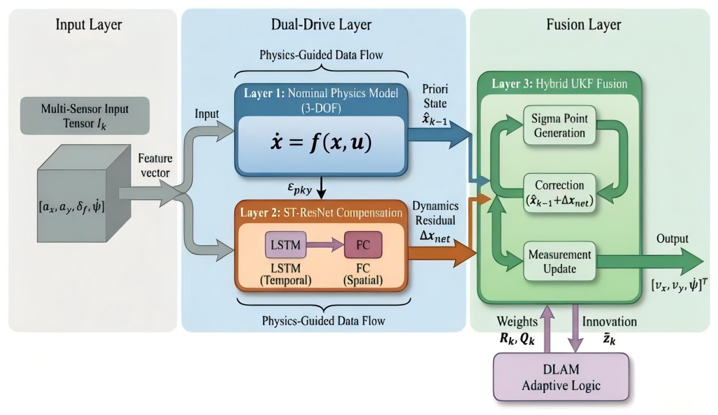
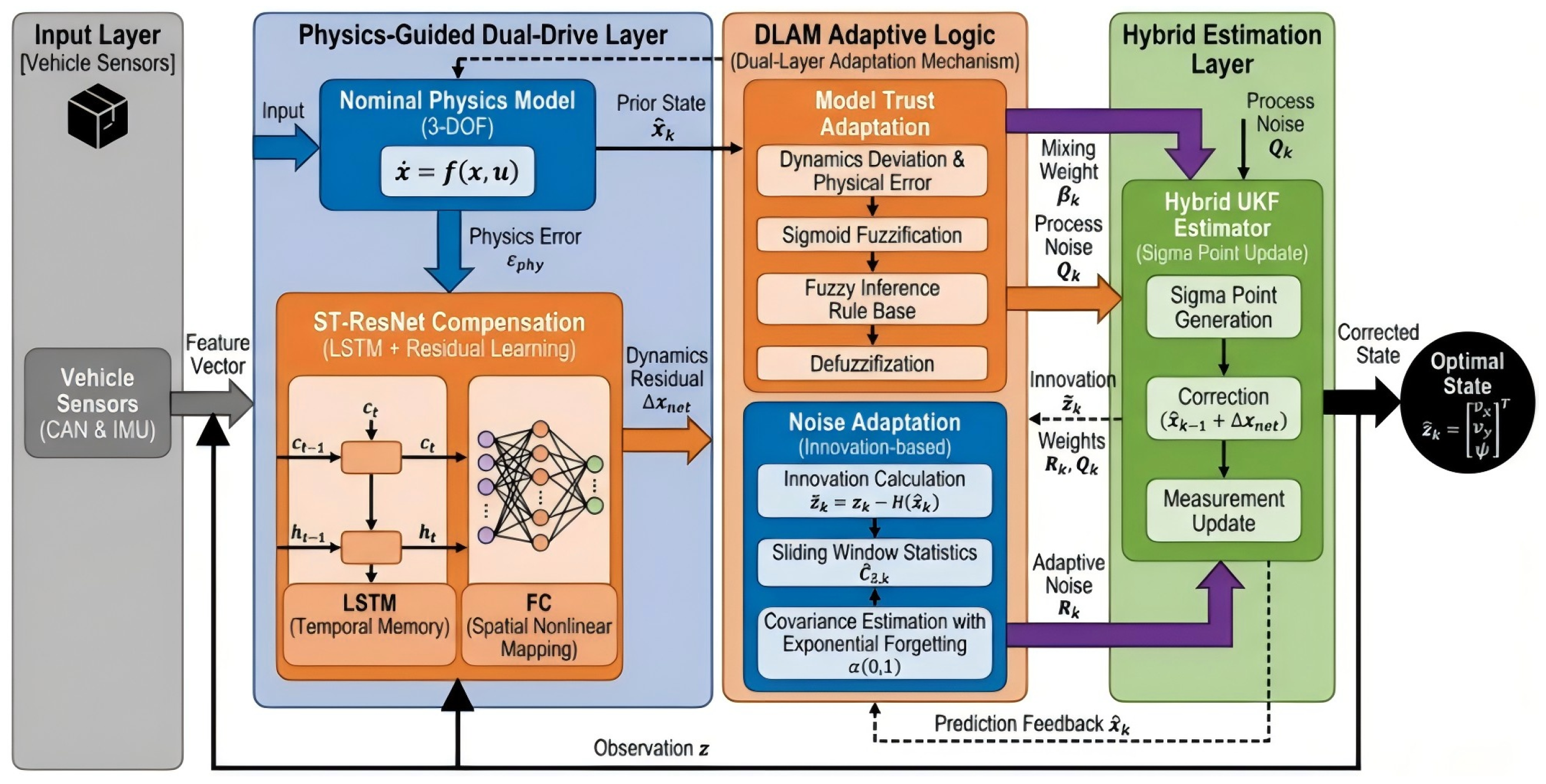
In response to the failure characteristics of the nominal model in the nonlinear region, this section proposes the PD-HEF architecture (Figure 3), adopting a parallel mode of Physical Skeleton+Data Patch. It utilizes an ST-ResNet to predict dynamic residuals and embeds them into the time update step of the unscented Kalman filter.

3.1. Construction of Spatio-Temporal Feature Coupled Residual Network (ST-ResNet)

This article establishes a mapping from the observable feature space to the implicit dynamic residual space: $\mathrm{M}$: ${\mathbf{I}}_t\to \mathsf{\Delta }{\mathbf{x}}_{net}$.

3.1.1. Physics-Guided Input Feature Construction

To enable the network to identify mechanism mismatch, the input feature vector ${\mathbf{I}}_k$ not only includes the current sensor observations and system control inputs, but also explicitly introduces the prediction error of the nominal physical model.

$${\mathbf{I}}_k=[{\mathbf{u}}_k,{\mathbf{z}}_k,{\mathsf{\epsilon }}_{phy,k}]$$

(11)

The last specially introduced term is the prediction error (${\mathsf{\epsilon }}_{phy}={\mathbf{z}}_k-h\left({\widehat{\mathbf{x}}}_{k\left|k-1\right.}^{nom}\right)$) of the physical model; ${\widehat{\mathbf{x}}}_{k\left|k-1\right.}^{nom}$ is the one-step prediction state of the pure physical model, and $h(·)$ is the observation function. This error term serves as a direction guide for the gradient descent, preventing the network from learning the basic kinematics that the physical model already knows.

3.1.2. Network Topology and Residual Output

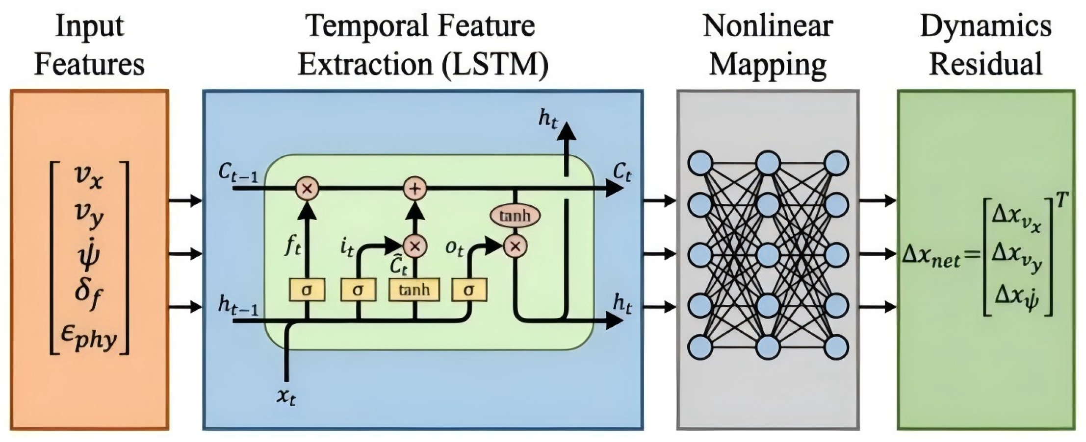
To address phase lag, an LSTM is used as the core feature extractor. The LSTM integrates historical lateral dynamics through a gating mechanism (Equations (12)–(17)), simulating the accumulation of tire deformation energy [33].

$$\begin{array}{cc}\hfill {\mathbf{f}}_t& =\sigma ({\mathbf{W}}_f·[{\mathbf{h}}_{t-1},{\mathbf{I}}_t]+{\mathbf{b}}_f)\hfill \end{array}$$

(12)

$$\begin{array}{cc}\hfill {\mathbf{i}}_t& =\sigma ({\mathbf{W}}_i·[{\mathbf{h}}_{t-1},{\mathbf{I}}_t]+{\mathbf{b}}_i)\hfill \end{array}$$

(13)

$$\begin{array}{cc}\hfill {\mathbf{O}}_t& =\sigma ({\mathbf{W}}_o·[{\mathbf{h}}_{t-1},{\mathbf{I}}_t]+{\mathbf{b}}_o)\hfill \end{array}$$

(14)

$$\begin{array}{cc}\hfill {\tilde{\mathbf{C}}}_t& =tanh({\mathbf{W}}_C·[{\mathbf{h}}_{t-1},{\mathbf{I}}_t]+{\mathbf{b}}_C)\hfill \end{array}$$

(15)

$$\begin{array}{cc}\hfill {\mathbf{C}}_t& ={\mathbf{f}}_t\odot {\mathbf{C}}_{t-1}+{\mathbf{i}}_t\odot {\tilde{\mathbf{C}}}_t\hfill \end{array}$$

(16)

$$\begin{array}{cc}\hfill {\mathbf{h}}_t& =tanh{\mathbf{C}}_t\odot {\mathbf{O}}_t\hfill \end{array}$$

(17)

where: $\sigma$ denotes the sigmoid activation function, with an output range of [0, 1]; $\mathbf{W}$ and $\mathbf{b}$ represent the weight matrices and bias vectors corresponding to the respective gates; ${\mathbf{f}}_t$ is the forget gate, which determines the extent to which information should be discarded from the cell state; ${\mathbf{i}}_t$ serves as the input gate, controlling the storage of new information into the cell state; ${\mathbf{O}}_t$ is the output gate, regulating the information output from the current cell state; ${\tilde{\mathbf{C}}}_t$ denotes the candidate cell state; ${\mathbf{C}}_t$ represents the updated cell state, which physically simulates the accumulation of tire deformation energy; ${\mathbf{h}}_t$ is the hidden state output; and ⊙ denotes the Hadamard product (element-wise multiplication).

LSTM units are used to capture temporal features and integrate historical lateral dynamics through gating mechanisms, compensating for the transient response distortion of the physical model at the moment of lane change switching. The network outputs a state increment correction vector $\mathsf{\Delta }{\mathbf{x}}_{net,k}$ in the discrete time domain (Equation (18)). Its physical meaning is to estimate the displacement deviation generated by the nominal model within the integral step size.

$$\mathsf{\Delta }{\mathbf{x}}_{net,k}\approx {\int }_t^{t+\mathsf{\Delta }t}{\mathbf{f}}_{res}\left(\tau \right)d\tau$$

(18)

The network topology of ST-ResNet is shown in Figure 4. This network is composed of a cascaded LSTM layer for extracting temporal historical memory and a fully connected layer for spatially nonlinear mapping.

In this paper, the detailed hyperparameter configuration of the ST-ResNet is listed in

Table 1. Hyperparameter settings of ST-ResNet.

Parameter	Value	Description
Input Dimension	6	${[v_x,a_y,{\delta }_f,\dot{\psi },\mathsf{\Delta }\dot{\psi },\mathsf{\Delta }\beta ]}^T$
LSTM Hidden Layers	2	Number of stacked LSTM layers
LSTM Hidden Units	128	Feature dimension in hidden state
FC Layers	3	Fully connected layers for spatial mapping
FC Neurons	[64, 32, 3]	Neurons in each FC layer
Activation Function	ReLU/Tanh	ReLU for FC, Tanh for LSTM internal
Learning Rate	0.001	Initial learning rate with decay
Batch Size	64	Number of samples per update
Epochs	200	Total training iterations
Dropout Rate	0.2	To prevent overfitting

. The network training was implemented based on the PyTorch (2.3.0) framework, utilizing the Adam optimizer for gradient descent.

3.1.3. Data Generation and Implementation Strategy

To ensure the ST-ResNet comprehensively learns the underlying physical mismatch rather than merely overfitting to specific trajectories, a massive and diverse dataset was systematically constructed using the CarSim-Simulink joint architecture.

Driving Conditions and Scope: The training maneuvers deliberately included high-excitation scenarios required to trigger tire saturation and load transfer mechanisms: standard double lane change (DLC), sine sweep (0.5 to 2.0 Hz), Fish-Hook, and Step Steering. The vehicle’s longitudinal velocity was dynamically traversed between 40 km/h and 120 km/h. Concurrently, the road adhesion coefficient ($\mu$) was uniformly distributed across a vast spectrum bounded between 0.3 (packed snow/ice) and 1.0 (dry asphalt).

Data Volume and Splits: The dataset amassed a total of 250,000 discrete sampling observations (recorded at a rigorous 10 ms resolution equivalent to chassis control cycles). The collected data samples were strictly partitioned into training (70%), validation (15%), and Extrapolation Testing (15%) sequences.

Ground Truth Residual Extraction: Within an actual automotive development cycle, the differential true states (${\dot{x}}_{true}$) would be captured by mounting extremely high-precision RTK-GNSS/INS systems onto proving-ground test vehicles. In this study, the integrated high-fidelity CarSim multibody engine mathematically substituted the physical test vehicle. The targeted learning residual $f_{res}$ was harvested purely offline by calculating the discrete error margin between the CarSim true state differential increment and the numerical derivative yielded simultaneously by the embedded 3-DOF nominal equations. This rigorous decoupling guarantees that the network operates strictly as an auxiliary compensator without overriding fundamental physical principles. Regarding the computational training cost, the generalized ST-ResNet offline synthesis was executed within a controlled NVIDIA RTX 3060 GPU environment. The entire propagation reliably converges under a 2.5 h threshold, which is extremely affordable during the OEM developmental phase.

3.2. Hybrid-UKF Closed-Loop State Update with Embedded Network Compensation

To address system noise and effectively integrate measurement information, the output of the ST-ResNet is injected into the prediction stage of the UKF through an extended hybrid evolution operator.

3.2.1. Hybrid Sigma-Point Evolution

At time step $k-1$, based on the posterior state estimation ${\widehat{\mathbf{x}}}_{k-1}$ and covariance ${\mathbf{P}}_{k-1}$, a set of $2L+1$ sigma points is generated (L is the dimension of the state vector). The one-step prediction of the state no longer relies solely on the physical equations; instead, it is composed of both a physical deduction term and a network compensation term.

$${\mathbf{Ø}}_{k\left|k-1\right.}^{\left(i\right)}=\underset{\mathrm{PhysicsEvolution}}{\underbrace{{\mathbf{Ø}}_{k-1}^{\left(i\right)}+\mathsf{\Delta }t·\mathrm{RK}4({\mathbf{f}}_{nom},{\mathbf{Ø}}_{k-1}^{\left(i\right)},{\mathbf{u}}_{k-1})}} + {\beta }_k·\underset{\mathrm{DataCorrection}}{\underbrace{\mathsf{\Delta }{\mathbf{x}}_{net}\left({\mathbf{I}}_{k-1}\right)}}$$

(19)

where: $\mathrm{RK}4(·)$ denotes the fourth-order Runge–Kutta numerical integration operator based on the nominal model; ${\beta }_k\in [0,1]$ represents the adaptive confidence weight, which will be defined in the subsequent section. This equation represents a vector-level fusion: the physical model provides the base trend while the neural network provides the differential correction.

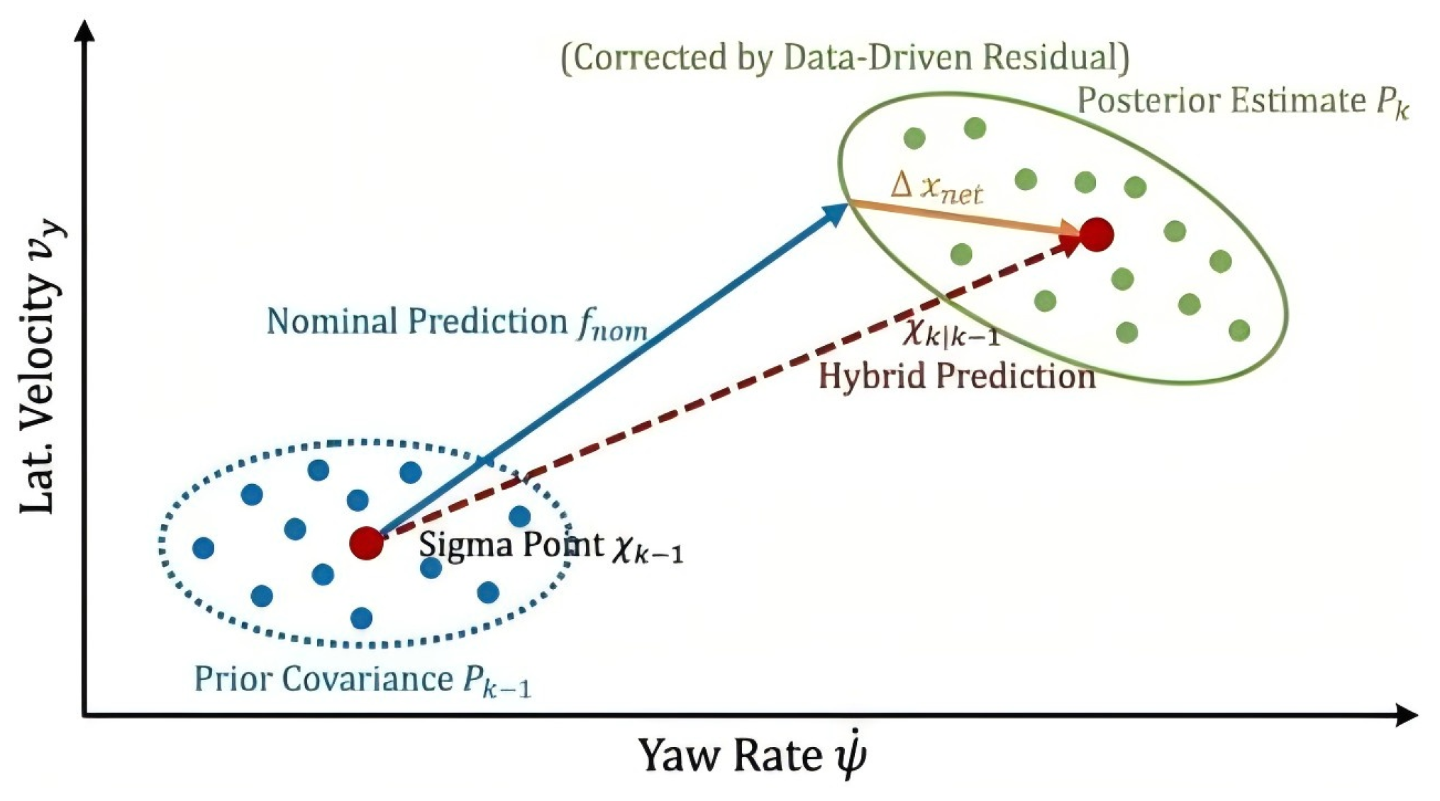
The conceptual mechanism illustrated in Figure 5 is mathematically grounded in the nonlinear Bayesian inference of the UKF. Relying solely on the numerical physical integration (represented by the blue vector in Figure 5) yields a structurally biased prediction. Due to the unmodeled tire relaxation dynamics defined earlier, this purely physical evolution forces the mathematical expectation (prior mean) to natively deviate from the true state. Consequently, the calculated prior probability density function (PDF) mathematically shifts away from the true systemic distribution space.

To justify the visual claim of correction, the statistical translation must be explicitly traced. As formulated in Equation (19), the injected dynamic residual $▵x_{net}$ (the orange vector) acts directly on the evolutionary trajectory of each individual sigma point. Subsequently, when deriving the a priori state mean via the weighted summation defined in Equation (20), this point-by-point data injection structurally executes a statistical expected-value translation. It forcefully neutralizes the deterministic integration bias and drags the global statistical expectation formally back into the highest-likelihood region of the true posterior probability envelope (the green ellipse). Thus, bridging the visualizations in Figure 5 with the equations explicitly verifies the estimator’s capability.

3.2.2. Calculation of Hybrid a Priori Statistical Characteristics

Based on the set of sigma points after hybrid evolution, the a priori state mean (${\widehat{\mathbf{x}}}_{k\left|k-1\right.}$) and the a priori covariance matrix (${\mathbf{P}}_{k\left|k-1\right.}$) are calculated as follows:

$$\begin{array}{cc}\hfill {\widehat{\mathbf{x}}}_{k\left|k-1\right.}& ={\displaystyle \sum _{i=0}^{2L}}{w_m}^{\left(i\right)}{\mathbf{Ø}}_{k\left|k-1\right.}^{\left(i\right)}\hfill \end{array}$$

(20)

$$\begin{array}{cc}\hfill {\mathbf{P}}_{k\left|k-1\right.}& ={\displaystyle \sum _{i=0}^{2L}}{w}_c^{\left(i\right)}\left({\mathbf{Ø}}_{k\left|k-1\right.}^{\left(i\right)}-{\widehat{\mathbf{x}}}_{k\left|k-1\right.}\right){\left({\mathbf{Ø}}_{k\left|k-1\right.}^{\left(i\right)}-{\widehat{\mathbf{x}}}_{k\left|k-1\right.}\right)}^T+{\mathbf{Q}}_k\hfill \end{array}$$

(21)

where: ${w_m}^{\left(i\right)}$ and ${w_c}^{\left(i\right)}$ are the weighting coefficients for the mean and covariance in the UKF, respectively. ${\mathbf{Q}}_k$ is the process noise covariance matrix, which is dynamically adjusted within the adaptive mechanism.

4. Dual-Layer Adaptive Mechanism Based on Condition Identification

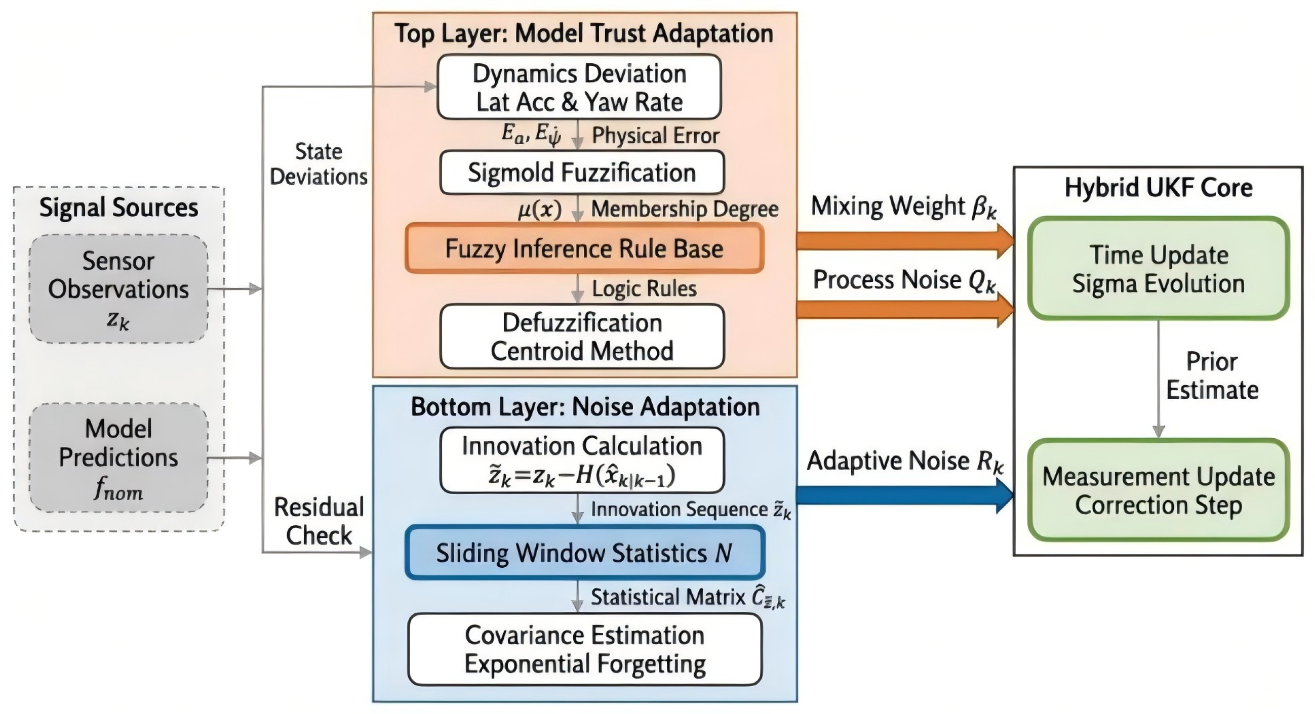
To sustain estimation performance across complex and variable working conditions where a single set of fixed parameters is insufficient, this section aims to construct a Dual-Layer Adaptive Mechanism (DLAM). The bottom layer focuses on environmental adaptability, resisting sensor noise interference, while the top layer focuses on dynamic authority allocation, dynamically scheduling trust weights between the physical model and the neural network.

4.1. Bottom-Layer Adaptation: Anti-Noise Strategy Based on Innovation Statistics

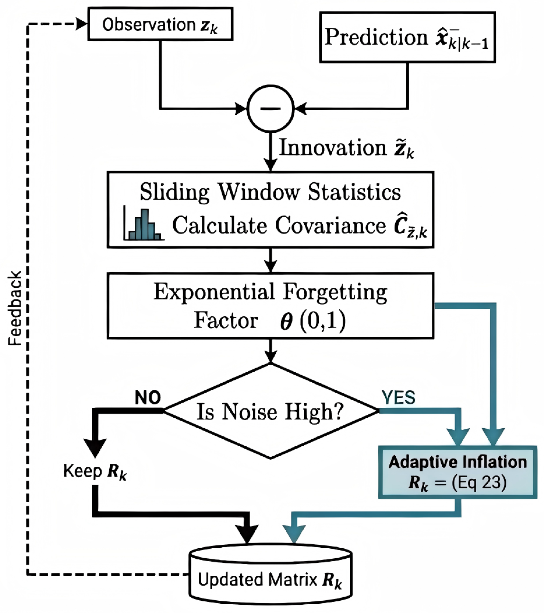
Addressing the issue where the statistical characteristics of sensor noise deviate from calibration values under harsh road conditions, an adaptive regulator for the observation noise covariance (${\mathbf{R}}_k$) is designed in the bottom layer based on the innovation sequence.

Define the innovation vector at time k as ${\tilde{\mathbf{z}}}_k={\mathbf{z}}_k-\mathbf{H}{\widehat{\mathbf{x}}}_{k\left|k-1\right.}$, which characterizes the discrepancy between the actual observation and the measurement prediction centered on the hybrid model. A sliding window is used to estimate the real-time covariance ${\widehat{\mathbf{C}}}_{\tilde{z},k}$ of the innovation. To balance the stability and sensitivity of the estimation, an exponential forgetting factor is introduced: $\theta \in (0,1]$.

$${\widehat{\mathbf{C}}}_{\tilde{z},k}=\theta {\widehat{\mathbf{C}}}_{\tilde{z},k-1}+(1-\theta )\left({\tilde{\mathbf{z}}}_k{{\tilde{\mathbf{z}}}_k}^T\right)$$

(22)

According to the principle of Kalman filtering, the theoretical innovation covariance should satisfy ${\mathbf{C}}_{\tilde{z},k}=\mathbf{H}{\mathbf{P}}_{k\left|k-1\right.}{\mathbf{H}}^T+{\mathbf{R}}_k$. From this, the adaptive update formula for the measurement noise covariance can be derived.

$${\mathbf{R}}_k=max({\mathbf{R}}_0,{\widehat{\mathbf{C}}}_{\tilde{z},k}-\mathbf{H}{\mathbf{P}}_{k\left|k-1\right.}{\mathbf{H}}^T)$$

(23)

where: ${\mathbf{R}}_0$ represents the initial noise baseline value calibrated by the sensor; $\mathbf{H}$ is the observation matrix.

As shown in Figure 6, when road excitation causes a drastic increase in sensor noise, the total variance of the innovation (${\widehat{\mathbf{C}}}_{\tilde{z}}$) increases. Consequently, the algorithm determines that measurement noise has increased and drives the inflation of ${\mathbf{R}}_k$. This subsequently reduces the Kalman gain, making the system rely more on the predicted values from the time update step, thereby suppressing the contamination of state estimation by observation noise.

4.2. Top-Layer Adaptation: Model Weight Scheduling Based on Fuzzy Logic

To dynamically regulate the confidence weight ${\beta }_k$ in Equation (19) and the process noise ${\mathbf{Q}}_k$ in Equation (21), a fuzzy logic scheduler is designed. The core logic is to prioritize the deterministic physical laws in the linear steady-state region while granting dominance to the neural network for trajectory correction as the vehicle approaches nonlinear stability limits where the physical model fails.

4.2.1. Selection of Dynamic Deviation Descriptors

To accurately identify the failure of the analytical model, the lateral acceleration residual $E_{ay}$ and the lateral dynamics intensity $I_{dyn}$ are selected as inputs for the fuzzy system:

$$E_{ay}=\left|a_{y,m}-a_{y,nom}\right|$$

(24)

where: $a_{y,nom}$ is calculated by the nominal 3-DOF model. This term directly quantifies the systematic deviations originating from neglected tire relaxation effects and load transfer, as analyzed in Section 2.1.

$$I_{dyn}=|a_{y,m}|/\phantom{|a_{y,m}|(\mu g}(\mu g)$$

(25)

This term represents the proximity of the vehicle to physical adhesion boundaries. Based on Jensen’s Inequality in Section 2.1, higher $I_{dyn}$ triggers tire force saturation, leading the nominal model to overestimate the stability limit via linear extrapolation.

4.2.2. Scheduling Rules and Output Calculation

The input spaces $E_{ay}$ and $I_{dyn}$ are each divided into three fuzzy subsets: [Small (S), Medium (M), Large (L)] using overlapping membership functions. The output variable ${\beta }_k$ also corresponds to three subsets. The fuzzy rule base established upon the physical failure logic is shown in

Table 2. Fuzzy rule base for ${\beta }_k$.

${\mathit{I}}_{\mathit{dyn}}$/${\mathit{E}}_{\mathit{ay}}$	Small (S)	Medium (M)	Large (L)
Small (S)	0.1 (Nominal)	0.2	0.3
Medium (M)	0.3	0.5	0.7
Large (L)	0.5	0.8	0.9 (Full Compensation)

.

The core physical logic of Table 2 is: when $I_{dyn}$ is small (linear steady-state region), the system highly trusts the physical equations (${\beta }_k\to 0.1$), regardless of minor residuals, thereby shielding against potential overfitting noise introduced by the neural network. Conversely, when both $I_{dyn}$ and $E_{ay}$ reach the Large (L) state, it indicates that the vehicle has entered the nonlinear limits and the physical model has failed severely. At this point, the network is granted the highest authority (${\beta }_k\to 0.9$), utilizing the high-order residual of ST-ResNet to forcibly correct the sigma-point evolution.

After defuzzification using the center of gravity method to obtain ${\beta }_k$, this output scheduling parameter essentially operates as a dual-role authority modulator within the generalized observer architecture. Primarily, it is immediately fed backward into the fundamental sigma-point evolution equation (refer back to Equation (19)). In this capacity, ${\beta }_k$ physically scales the injected data-driven correction magnitude $▵x_{net}\left({\mathbf{I}}_{\mathbf{k}-\mathbf{1}}\right)$, explicitly dictating how aggressively the neural network overrides the deterministic physical trajectory constraints.

Concurrently, functioning as its secondary mathematical role, the adaptive process noise covariance corresponding to the nonlinear boundaries is dynamically configured as follows:

$${\mathbf{Q}}_k={\mathbf{Q}}_0[1+\gamma ·{\beta }_k]$$

(26)

where ${\mathbf{Q}}_0$ is the base process noise matrix and $\gamma$ is the inflation coefficient. The physical essence of Equation (26) is that when the system identifies the failure of the physical model (${\beta }_k$ increases), it not only increases the proportion of data-driven compensation but simultaneously inflates the process noise ${\mathbf{Q}}_k$. This forces the Kalman gain to increase, making the filter more agile in responding to the residual correction signals. Through this closed loop, the system achieves an optimal game-theoretic balance between deterministic physical laws and flexible data compensation across all operating conditions.

Figure 7 fully illustrates the logical interaction closed loop of the DLAM. Through this dual-layer mechanism, the PD-HEF framework achieves an optimal dynamic balance between physical determinism and data flexibility across the full range of working conditions.

In summary, the DLAM mechanism not only provides a robust shell for the PD-HEF framework to cope with unknown noise environments but also resolves the issue of gaming weights between the physical model and the neural network in different motion modes through a knowledge-driven approach. This significantly enhances the survivability of the estimation framework under vehicle limit boundary conditions. The complete framework of the hybrid-driven vehicle state estimation is shown in Figure 8.

5. Simulation Experiments and Result Analysis

To verify the effectiveness and robustness of the proposed Physically-Driven Hybrid Estimation Framework (PD-HEF) under complex dynamic conditions, this chapter conducts experimental validation based on a CarSim(2020) and MATLAB/Simulink (R2023b) joint simulation platform. The experimental design progresses from the unit level to the system level, and from steady-state dynamics to limit-handling conditions, comparing the following three schemes: traditional Physics-Driven UKF (Phy-UKF), pure data-driven LSTM (Pure-LSTM), and the proposed hybrid framework (PD-HEF).

5.1. Simulation Platform Construction

The vehicle parameters tested in this article are selected from CarSim, with parameters shown in

Table 3. Vehicle parameters.

Description	Symbol	Values
Vehicle mass	m	1440 kg
Yaw moment of inertia	$I_z$	1523 kg·m2
Distance from the front axle to CG	$l_f$	1.16 m
Distance from the rear axle to CG	$l_r$	1.71 m
Wheel track	B	1.57 m
Centroid height	$h_g$	0.64 m
Rolling radius of the wheel	$R_e$	0.30 m
Wheelbase	L	2.87 m

. To simulate the physical characteristics of real onboard sensors, non-Gaussian white noise was injected into the sensor signals output by CarSim (longitudinal acceleration $a_x$, yaw rate $\dot{\psi }$, steering wheel angle ${\delta }_f$), and a 10 ms CAN bus signal transmission delay was considered. (Note: although the internal calculations of the algorithm are performed in radians consistent with the logic of the dynamic equations, some of the simulation results in the figures are converted to degrees for better visualization and engineering intuition).

To quantitatively evaluate the differences in dynamic tracking performance among different methods, the root mean square error (RMSE) is selected as the core evaluation metric. RMSE can effectively penalize large prediction deviations and reflect the comprehensive accuracy of the estimator over the entire time domain:

$$\mathrm{RMSE}=\sqrt{{\displaystyle \frac{1}{N}}{\displaystyle \sum _{k=1}^N}{({\widehat{x}}_k-x_k^{GT})}^2}$$

(27)

where: N is the total number of sampling points, ${\widehat{x}}_k$ is the estimated state value at time k, $x_k^{GT}$ is the corresponding CarSim ground truth.

5.2. ST-ResNet Network Training Performance Analysis

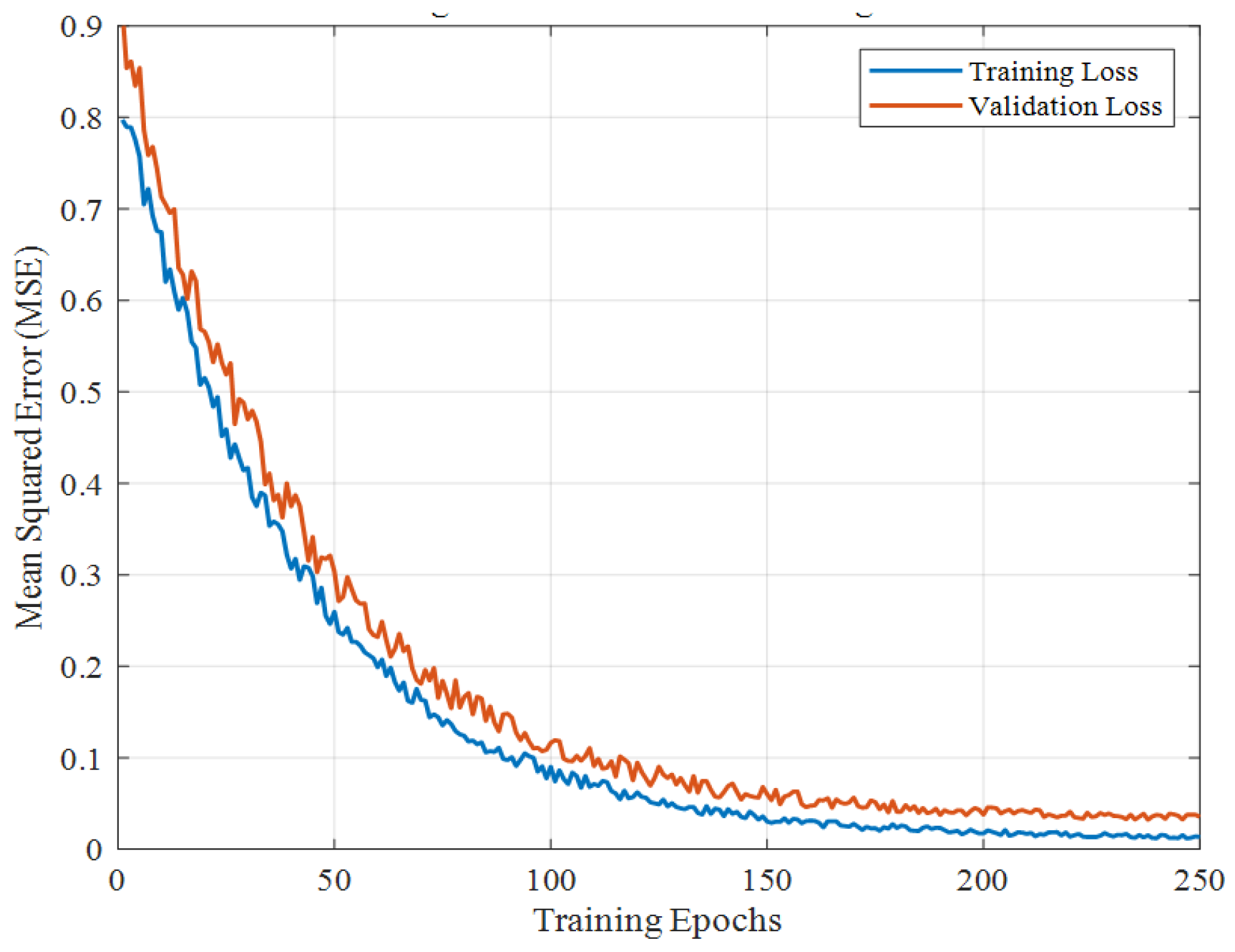
Offline performance assessment of the ST-ResNet occurred prior to its integration into the UKF loop. This step verified the capability of the network to generalize mechanism mismatch terms. Training convergence (MSE loss) appears in Figure 9. Rapid reduction in training loss is evident, reaching the 10-3 magnitude within nearly 150 epochs. Validation loss drops simultaneously and remains steady near 0.05, showing no severe divergence.

Meanwhile, the test set loss is slightly higher than the training set and exhibits minor oscillations. This indicates that the network has not overfitted and possesses a certain degree of generalized anti-noise capability.

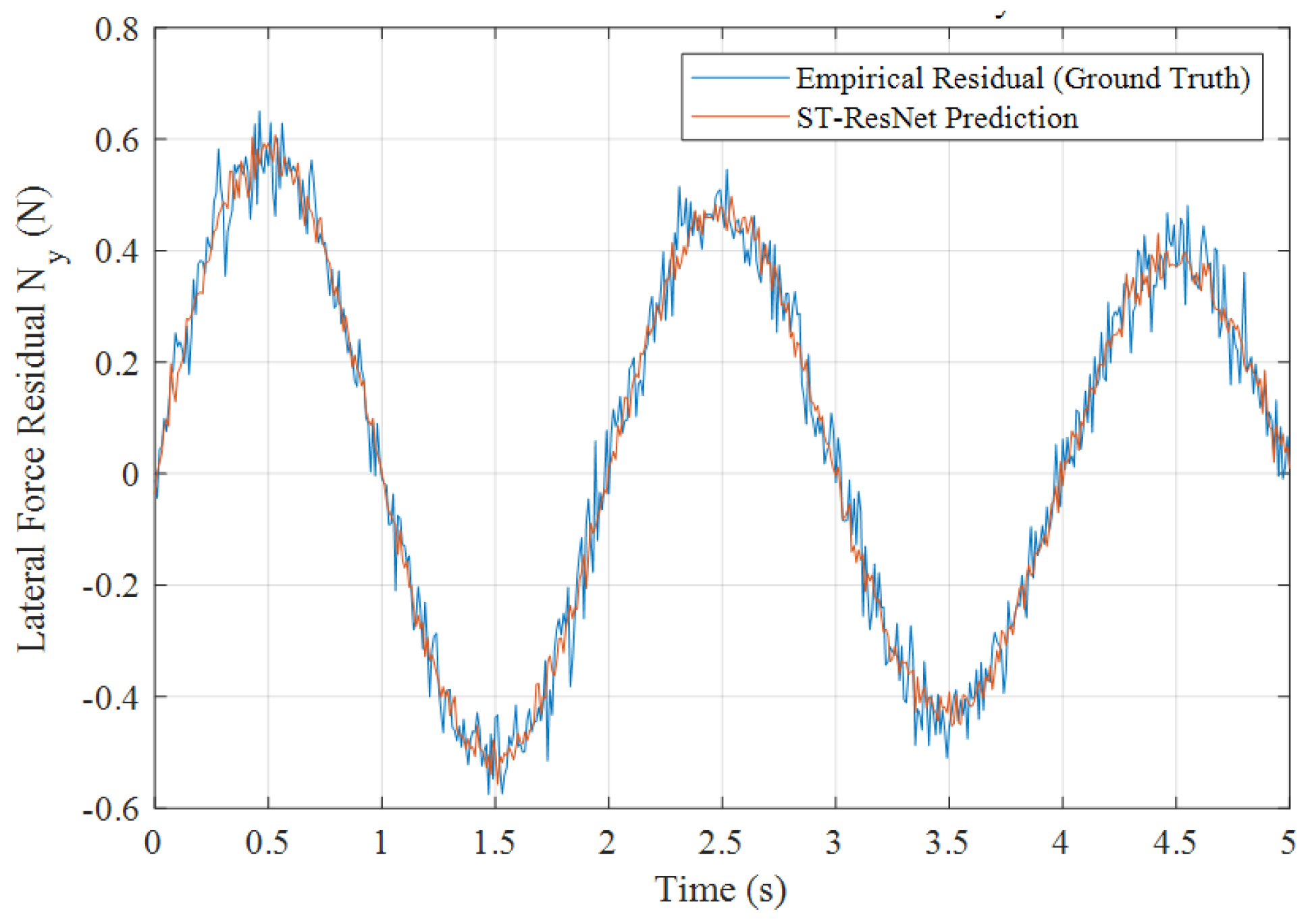
Figure 10 further verifies the learning effect of the network on the dynamic residual term from a physical perspective. In the figure, the blue solid line represents the empirical residual calculated by back-calculating the CarSim ground truth (the difference between the true physical value and the nominal model value), which contains obvious high-frequency measurement noise. The orange solid line is the prediction output of ST-ResNet. The analysis indicates that ST-ResNet does not mechanically memorize high-frequency measurement noise but successfully extracts the implicit dynamic residual trend. Physically, this trend corresponds precisely to the systematic deviation produced by the nominal model due to parameter perturbation and simplifying assumptions (such as unmodeled tire nonlinearities).

5.3. Simulation Analysis Under Limit-Handling Conditions

To systematically evaluate the estimation performance of the proposed PD-HEF framework regarding time-domain transient responses and spatial nonlinear boundaries, this section conducts two representative limit test scenarios: high-adhesion high-speed double lane change (High-Adhesion High-Speed DLC) and Low-Adhesion Variable-Frequency Sine Sweep.

It is critical to note that while validating the aforementioned algorithm advantages, the strictly open-loop analytical performance of the foundational 3-DOF model (i.e., pure integration entirely lacking recursive UKF measurement feedback updates) is purposively omitted from graphical plotting superposition. Under boundary-testing nonlinear scenarios, the unconstrained lack of load transfer decoupling forces the pure open-loop model simulation to exhibit severe integral wind-up trajectory divergence (e.g., projecting lateral acceleration trajectory offsets exceeding 80% margins under the $\mu =0.3$ sweep test). Attempting to plot this mathematical divergence identically alongside the filtered algorithms would disproportionately expand the scale of Cartesian Y-axis axes, visually flatlining the transient evaluation disparities surrounding the PD-HEF curve and ground truth parameters. Therefore, the implemented fixed-parameter ‘Phy-UKF’ line in the succeeding analyses fundamentally represents the theoretical ‘best-case scenario’ limit for traditional mechanic methodology algorithms functioning against such harsh dynamic bounds.

5.3.1. High-Adhesion High-Speed Double Lane Change (DLC)

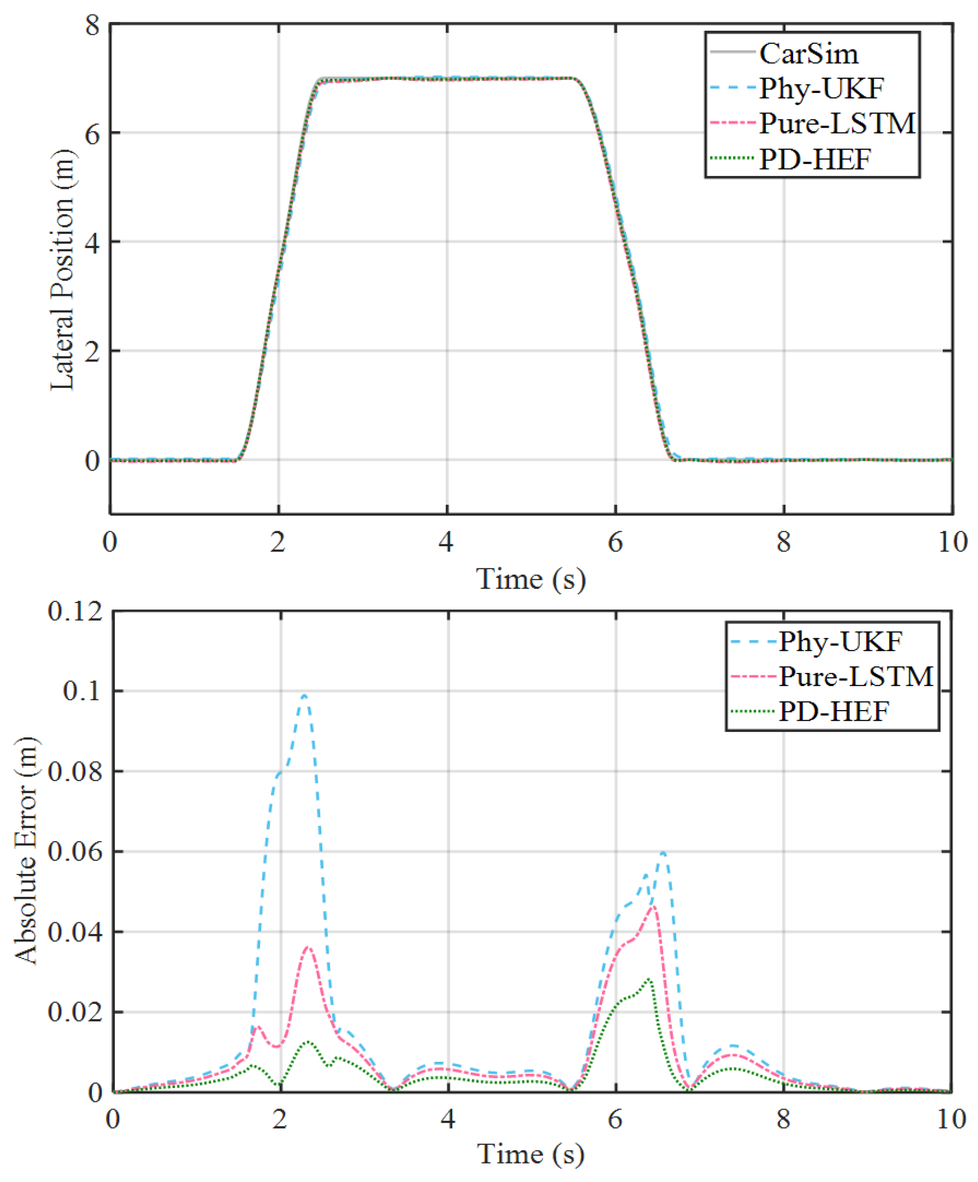
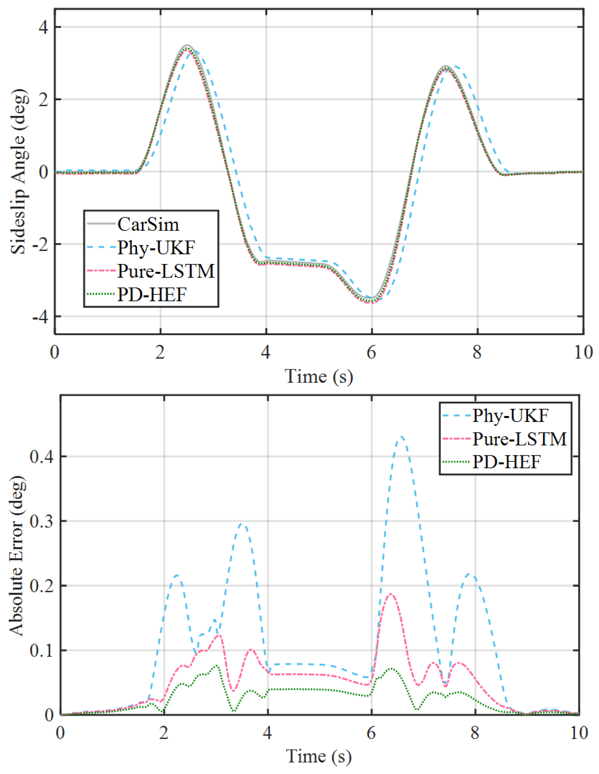
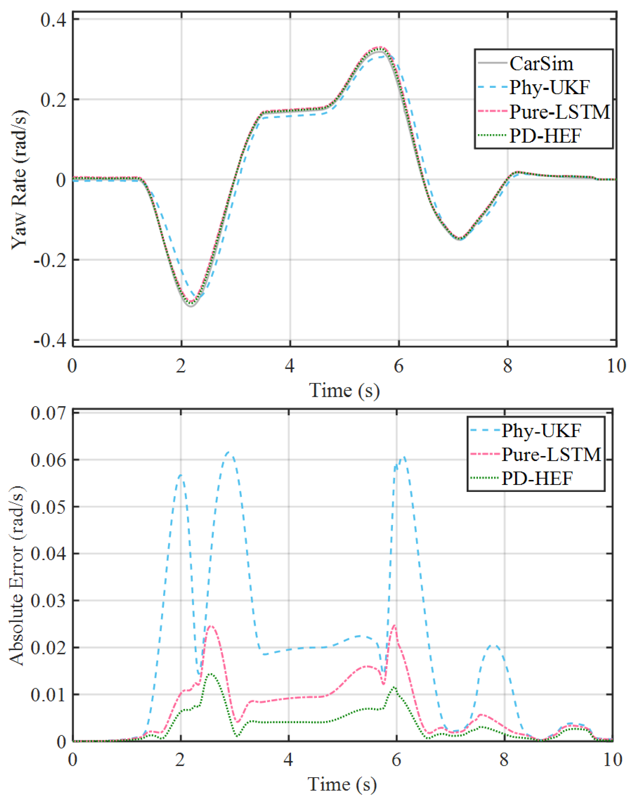
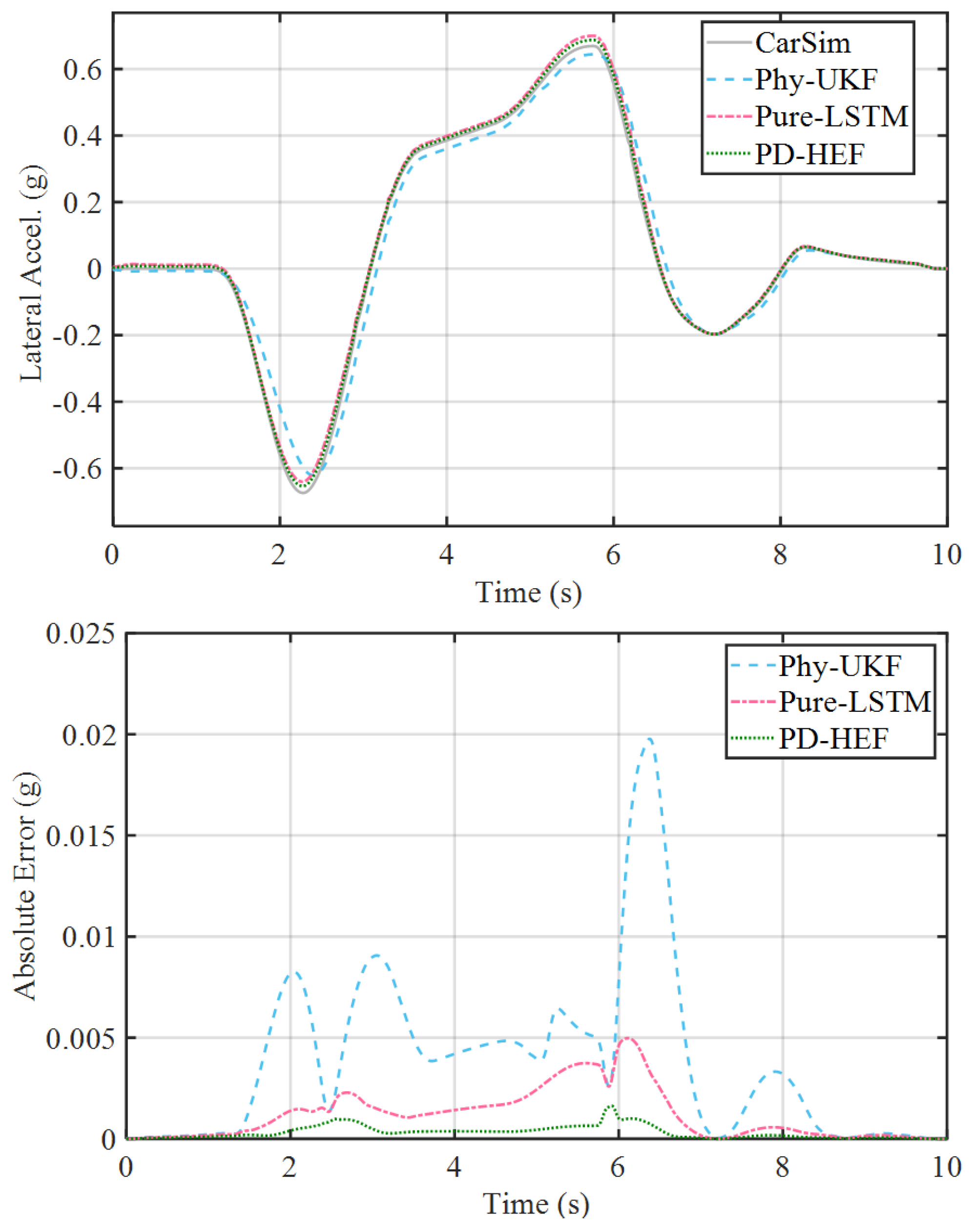
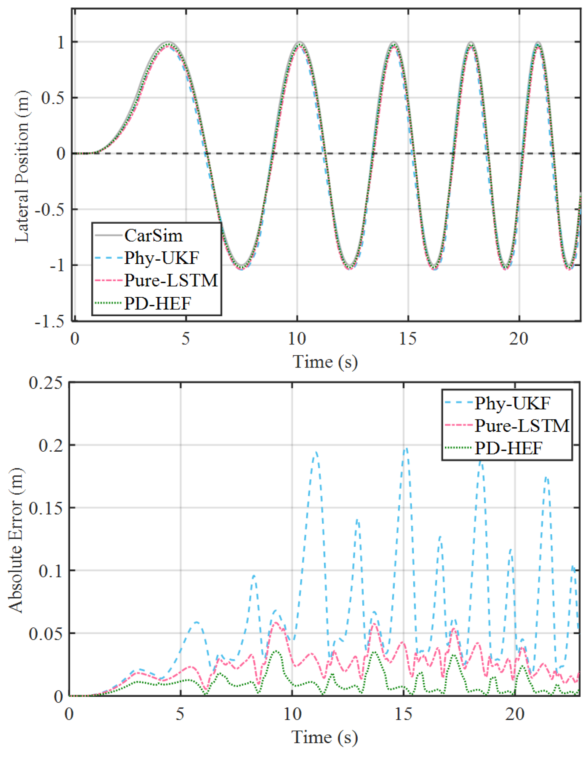
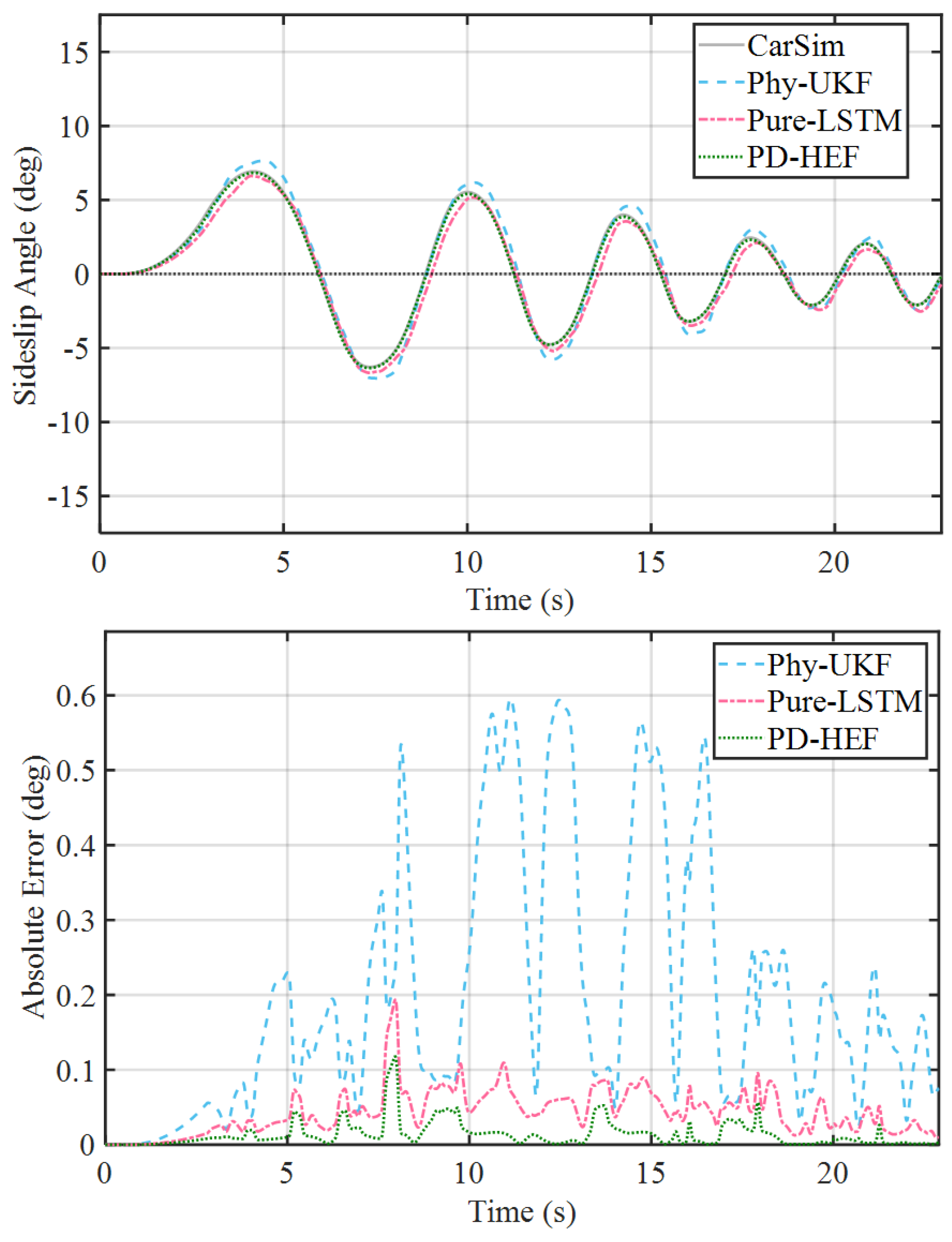
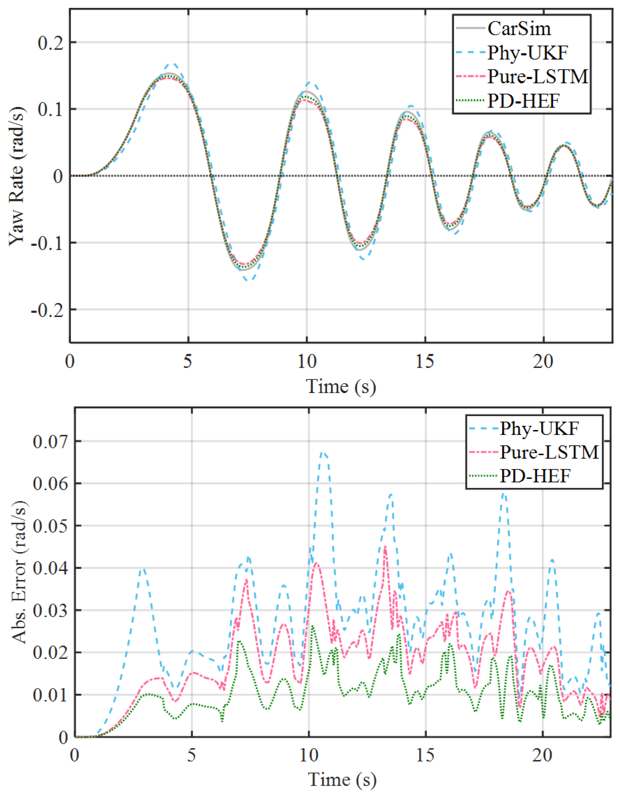
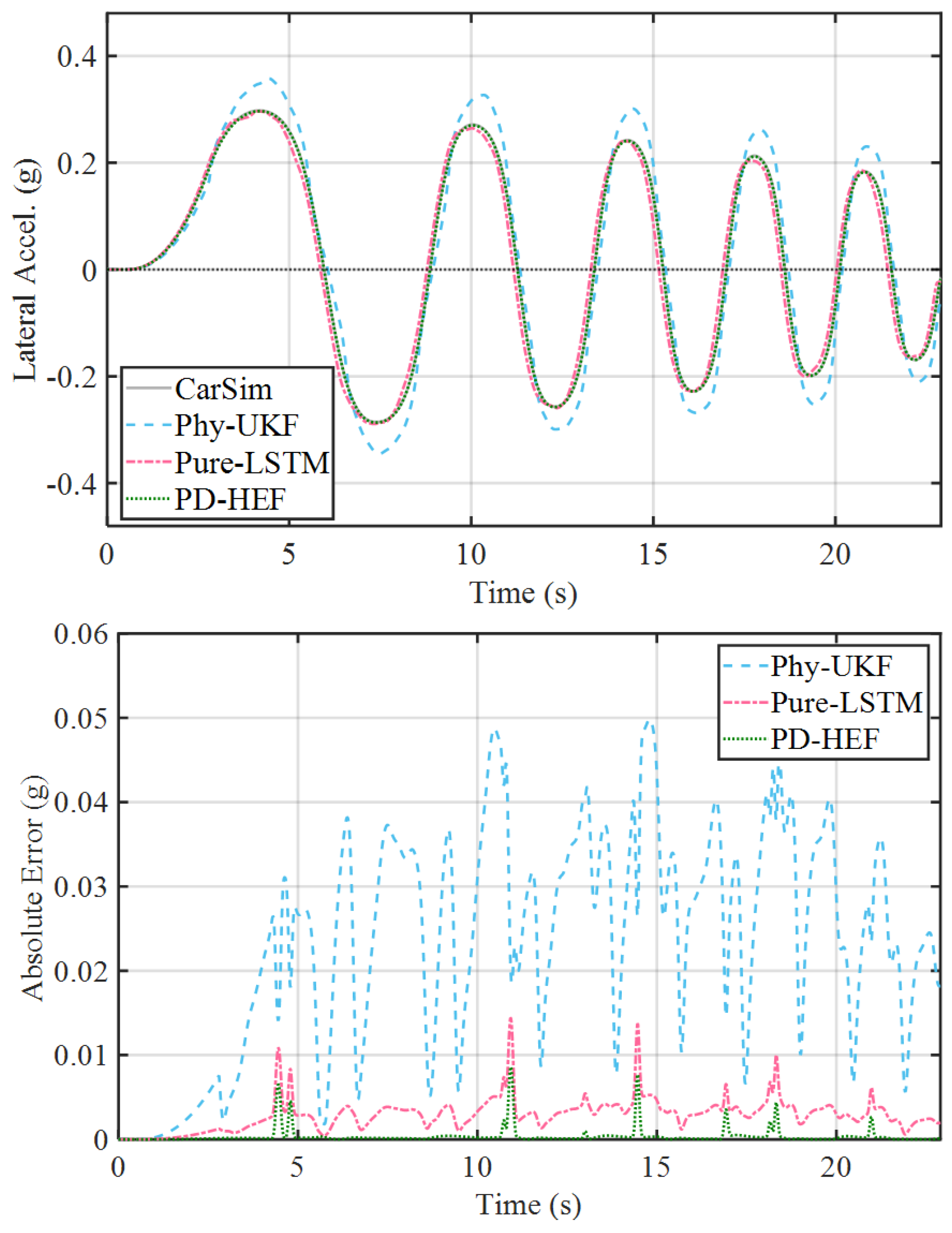
Standard ISO-3888-2 [34] DLC tests were performed with a road adhesion coefficient of $\mu =0.85$ and a constant longitudinal velocity of 100 km/h. Under these conditions, the lateral acceleration peak rapidly approaches 0.7 g, subjecting the vehicle to severe transient lateral excitation. The core target of this test isolates the compensation quality for the tire relaxation length. The simulation results are presented in Figure 11, Figure 12, Figure 13 and Figure 14.

(1) Transient Phase Characteristics: Based on the plotted CG sideslip angle (Figure 12) and yaw rate (Figure 13) within the 3 s to 6 s window, severe dynamic hysteresis occurs in the Phy-UKF baseline. Peak signal matching fails drastically compared to ground truth (grey solid line), leading to surging absolute errors. The steady-state assumption of the classical magic formula drives this structural fault. It forces an instant lateral force update relative to the slip angle, completely stripping away the contact patch deformation delay (Equation (5)).

(2) Smoothness and Amplitude Error of Data-driven Approach: The Pure-LSTM (red dotted line) leverages its gating mechanism to capture delay features in the time series, resulting in a phase that aligns much closer to the ground truth than the Phy-UKF. Furthermore, it maintains good curve smoothness without exhibiting the non-physical high-frequency oscillations often associated with raw data-driven methods. However, observing the simulation curve and absolute error curve of lateral acceleration in Figure 14, the Pure-LSTM demonstrates a certain Amplitude Mismatch at the extremal points. This is attributed to the tendency of pure neural networks to regress towards the mean distribution of the training data, leading to conservative estimation at the peaks and an inability to perfectly reproduce the full dynamic gain at the stability limits.

(3) Time-Domain Dynamic Compensation of PD-HEF: In contrast, the PD-HEF (green dotted line) demonstrates optimal transient tracking performance. Leveraging the ST-ResNet to learn from the physical prediction error as a priori knowledge, the architecture accurately predicts the dynamic mechanical residuals caused by the relaxation effect. As evident across the state curves in Figure 11, Figure 12, Figure 13 and Figure 14, the PD-HEF not only overcomes the phase lag of the Phy-UKF but also achieves sharper and more precise peak capture than the Pure-LSTM. Quantitative data indicates that the PD-HEF significantly reduces the RMSE of the sideslip angle and yaw rate, proving that injecting dynamic residuals into the physical model skeleton achieves the optimal reconstruction of transient vehicle dynamics.

5.3.2. Low-Adhesion Variable-Frequency Sine Sweep

To verify the algorithm’s robustness in strongly nonlinear regions, an icy road surface ($\mu =0.3$) and a medium speed (60 km/h) were selected for a sine sweep test with increasing frequency (0.6∼1 Hz). As the excitation amplitude increases, the tire lateral force gradually enters the saturation region. This scenario focuses on the estimator’s correction capability under Severe Model Mismatch. The results are shown in Figure 15, Figure 16, Figure 17 and Figure 18.

(1) By analyzing the sideslip angle of the center of mass in Figure 16 and the lateral acceleration in Figure 18, it can be seen that under the condition of sinusoidal input frequency increasing, the real state of the vehicle (gray solid line) shows typical adhesion saturation characteristics, which proves that the tire begins to enter the adhesion limit area. However, the Phy-UKF observer (blue dotted line) is limited by its unconstrained linear extrapolation mechanism, which leads to the linear overshoot phenomenon that the output of the algorithm significantly deviates from the reference true value. In particular, when the true sideslip angle in Figure 16 is stable at the saturation value, the theoretical estimate still keeps rising, significantly overestimating the stability boundary. The basic mechanism is that the nominal model ignores the load transfer caused by roll motion.

(2) Under the condition of sinusoidal frequency increasing input, the pure data-driven LSTM network (red dotted line) shows good nonlinear fitting ability, and its output basically conforms to the real saturation trend. By observing the position trajectory in Figure 15, it can be seen that due to the full coverage of the underlying training samples, the network has not yet experienced significant integral divergence and trajectory drift; However, when the state variables approach the extreme point, the absolute estimation deviation is still higher than the fusion architecture proposed in this paper. In contrast, PD-HEF (green dotted line) profoundly verifies the underlying value of physical a priori guidance. As the network input, the physical prediction error (${\mathit{\epsilon }}_{phy}$) acts as an explicit feature to characterize the instability of the observer, and can accurately define the trigger critical point of the dynamic failure interval. At this time, ST-ResNet outputs the corresponding reverse compensation residual, forcibly pulls back the divergent state evolution trajectory from the mechanism level and converges to the real nonlinear envelope. Combined with the observation of the deviation curve in Figure 18, the lateral acceleration error band extracted by the PD-HEF algorithm is greatly narrowed, and the output accuracy is highly close to the reference true value. The above quantitative results fully show that PD-HEF avoids the simple state weighted average mechanism; the core of the algorithm is that the trajectory is kept smooth in the linear dominant steady-state region by relying on the physical model, and the physical fault is corrected by the data residual in the limit region, so as to realize the precise decoupling and reconstruction of vehicle dynamics in the global region.

5.4. Deep Mechanistic Analysis of Physics-Data Interaction and DLAM Synergy

This section explores the inherent logic of the PD-HEF framework in handling stability-limit states from the perspectives of nonlinear dynamic evolution and Bayesian inference theory.

5.4.1. Decoupling and Physical Reconstruction of Spatio-Temporal Residuals

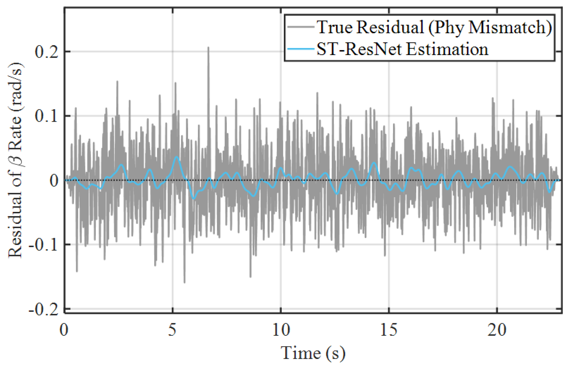
The failure of the nominal physical model is mainly due to the limitations of its unmodeled dynamic parameters. It can be seen from the data in Figure 19 that the dynamic residuals of ST-ResNet output (−0.03 to 0.04 rad/s) are by no means random random noise in disorder, but an intuitive mapping of the lateral force lag phenomenon analyzed in Section 2.2. Thanks to the deep time series correlation constructed in the time domain, the LSTM network effectively captures the accumulation process of strain energy in the tire, and then accurately compensates for the relaxation length effect, which is difficult to characterize by the steady-state magic formula. In the state recurrence stage of hybrid UKF, the above fusion mechanism not only ensures that the sampling of sigma points is strictly limited within the Newtonian dynamics framework, but also relies on the synchronous embedding of data residuals and the real evolution law of transient forces, so as to completely eliminate the phase-lead and lag errors in the traditional estimation.

5.4.2. Innovation Statistics and Information Entropy Balance in Feature Space

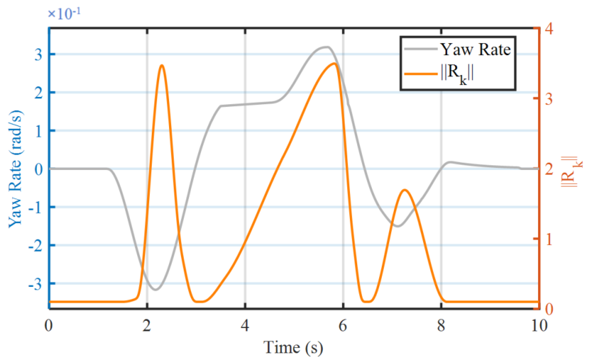
The bottom-layer adaptation demonstrates the Bayesian response of the estimator to observational uncertainty. Figure 20 shows that the estimator maintains robustness even during periods of intense yaw rate fluctuations. The underlying mechanism is that when sensors encounter non-Gaussian disturbances, the statistical properties of the innovation sequence deviate from theoretical expectations, triggering an inflation of the $∥R_k∥$ matrix norm from 0.1 to over 3.5. This adaptive regulation allows the PD-HEF to suppress the impact of measurement outliers on the state trajectory, ensuring kinematic continuity and physical consistency, which prevents the regression divergence common in pure data-driven methods.

5.4.3. Instantaneous Model Credibility Evaluation Under Logic Game

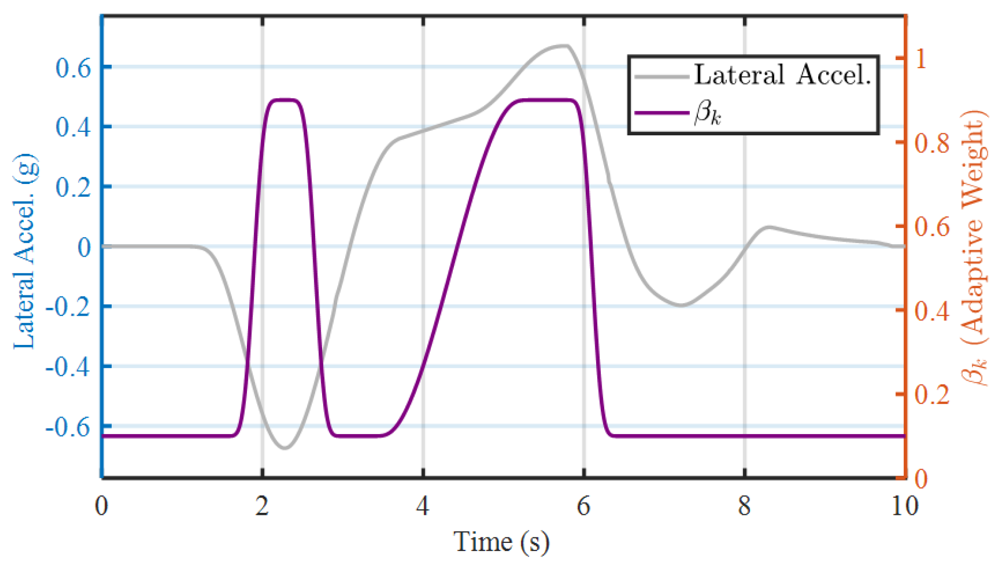
The top-layer mechanism (DLAM-Top) embodies the weight trade-off between physical determinism and data agility. Figure 21 exhibits a characteristic S-shaped transition of the confidence weight ${\beta }_k$ (from 0.1 to 0.9) once lateral acceleration $a_y$ exceeds the linear threshold. This reflects the system’s identification of the saturation mechanism in lateral dynamics: at high $a_y$, load transfer triggers the force attenuation described by Jensen’s Inequality, rendering the nominal physical model “blind” to the stability limits. Consequently, a weight of ${\beta }_k\approx 0.9$ grants the neural network dominant authority to rectify the physical trajectory. This soft-switching mechanism preserves physical determinism under steady states while forcibly correcting the linear overshoot of physical equations at limit boundaries through data-driven mappings, achieving an optimal estimation across the entire time domain.

5.4.4. Theoretical Necessity of the Adaptive Stability Mechanism

While the precision of the proposed framework is largely attributed to the residual compensation by ST-ResNet, the DLAM acts as a critical “firewall” for closed-loop stability. Based on the derivation of the Kalman filter, the Kalman gain matrix ${\mathbf{K}}_k$, which determines the correction strength, is inversely proportional to the measurement noise covariance ${\mathbf{R}}_k$ (${\mathbf{K}}_k\propto {{\mathbf{R}}_k}^{-1}$). In a conventional fixed-parameter filter/observer like Phy-UKF or Pure-LSTM, the system cannot adapt to sudden environmental changes. When the vehicle encounters harsh road impacts causing a surge in sensor noise variance, a fixed filter ignores the degradation of signal quality and maintains a high gain ${\mathbf{K}}_k$, thereby injecting measurement outliers directly into the state estimation. This leads to severe signal chattering or divergence. In contrast, the bottom layer of DLAM explicitly monitors the innovation sequence; upon detecting statistical anomalies, it dynamically inflates ${\mathbf{R}}_k$, mathematically forcing a reduction in ${\mathbf{K}}_k$. This theoretical behavior proves that in a hybrid-driven framework, the system requires not only the “accuracy” provided by deep learning but also the “statistical robustness” guaranteed by the adaptive mechanism.

5.5. Comprehensive Statistical Error Analysis and Real-Time Feasibility Evaluation

To quantitatively verify the comprehensive performance of the PD-HEF framework in terms of the time-domain transient response and spatial nonlinear boundary, this section calculates the RMSE under two different conditions and evaluates the single-step duration.

5.5.1. Global Accuracy Analysis of Dynamic State Estimation

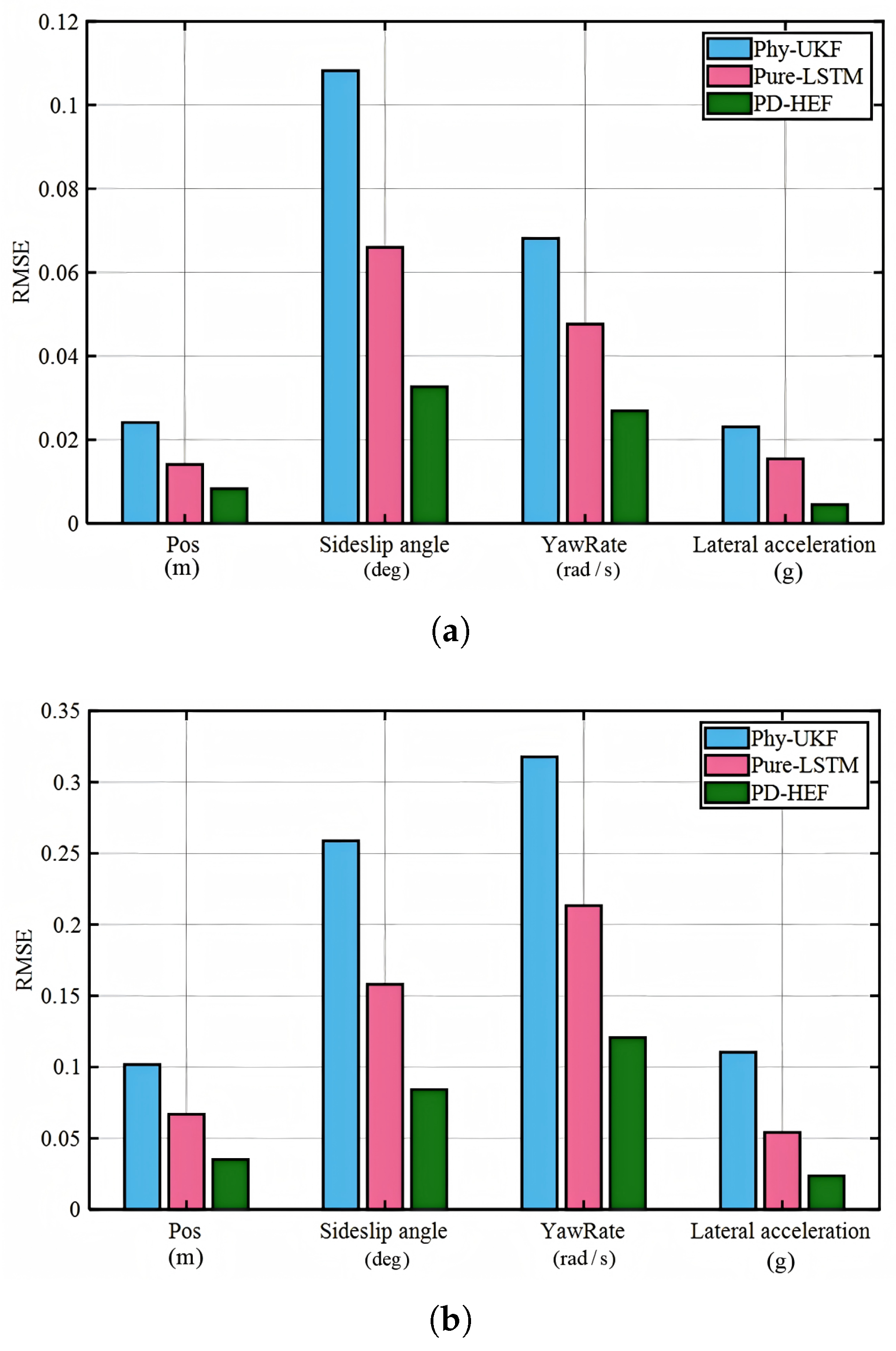
Figure 22 illustrates the error statistics for (a) high-adhesion double lane change (DLC) and (b) low-adhesion limit sine sweep scenarios.

High-adhesion double lane shifting condition: in the high-speed, high-adhesion, double lane shifting test condition, due to the tire relaxation effect not reflected in the physical model, Phy-UKF has a significant dynamic lag problem, resulting in the root mean square error (RMSE) value of vehicle position information (Pos) of 0.025 m and the RMSE value of yaw rate of 0.068 rad/s. The PD-HEF using ST-ResNet for accurate residual compensation significantly reduced these errors to 0.008 m (reduced by 60%) and 0.026 rad/s (reduced by 62%), respectively. Although there is obvious load transfer under this condition, PD-HEF can still keep the sideslip angle RMSE within the safe threshold of 0.033°, which effectively improves the accuracy of dynamic estimation.

Low-adhesion sinusoidal input condition: as shown in Figure 22b, on the low-adhesion road, tire force saturation makes the linear extrapolation of Phy-UKF invalid, resulting in the root mean square error (RMSE) of the sideslip angle increased to 0.26°. PD-HEF shows excellent boundary constraint ability, which is compressed to 0.08° by hybrid Kalman update, and the estimation error of lateral acceleration is kept at a low level of 0.025 g.

5.5.2. Computational Complexity and Real-Time Engineering Validation

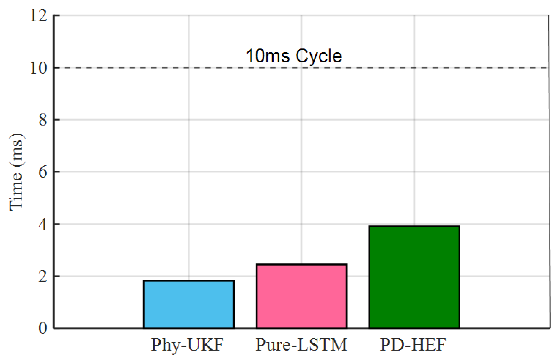
It is methodologically critical to elucidate that the aforementioned calculation speeds are explicitly benchmarked within a Personal Workstation environment (running MATLAB/Simulink (R2023b)) hosted on an Intel Core i7-12700H CPU @ 2.30 GHz with 16 GB RAM, Intel Corporation, Santa Clara, CA, USA) rather than a finalized, in-vehicle embedded microcontroller target. Inherently, equating floating-point MATLAB execution durations directly to dedicated automotive microcontrollers represents a conceptual incongruity. However, as shown in Figure 23, achieving an unoptimized loop computation timing of merely 4.0 ms per step serves as a highly robust viability metric. Given that conventional commercial chassis Domain Control Units (DCUs) dictate strict real-time cyclic update thresholds capped between 10 ms (100 Hz) and 20 ms limits (50 Hz), preserving an internal 4.0 ms timing loop successfully converts theoretical computational redundancy into a massive latency margin. This indicates that the fundamental bridging of analytical skeleton equations and dynamic residual networks is structurally edge-feasible for ensuing C-code deployment procedures targeting mass-production autonomous pipelines.

Although the single-step execution time has increased by about 2.1 ms, the total delay of 4.0 ms is still lower than the upper limit of the 10 ms control cycle normally required by the vehicle controller (indicated by the dotted line). This confirms that the framework successfully converts acceptable computational redundancy into critical observation accuracy.

6. Conclusions

This paper proposes a Physics-Driven Hybrid Estimation Framework (PD-HEF) that deeply couples physical models with deep residual learning. Based on theoretical modeling, network architecture design, and joint simulation validation, the main conclusions are drawn as follows.

(1) Physics-Guided Residual Decoupling Mechanism: Analytical gaps created by omitted relaxation length and vertical load shifting were isolated and quantified. Using pure kinematic prediction errors as an optimization target, the ST-ResNet successfully outputs discrete physical correction increments (contained strictly within [−0.03, 0.04] rad/s). Because of this configuration, time-domain phase tracking completely avoids traditional analytical observer lag.

(2) Dynamic Robustness via Dual-Layer Adaptive Architecture: The DLAM mechanism significantly enhances the system’s environmental adaptability. The bottom-layer filter, based on innovation statistics, effectively shields against interference by inflating the $∥R_k∥$ matrix to over 3.0 when measurement noise surges. Meanwhile, the top-layer fuzzy logic achieves smooth scheduling of the model confidence weight ${\beta }_k$ from the linear deterministic region (0.1) to the nonlinear limit region (0.9), ensuring optimal game-theoretic balance across different operational modes.

(3) Real-Time Algorithmic Feasibility: Tracking accuracy metrics jumped significantly, locking the sideslip angle RMSE to 0.08° and bounding lateral acceleration errors at 0.025 g during nonlinear tire saturation. At the execution level, overall inference requires merely 4.0 ms per step. This computation delay sits well below the 10 ms cycle mandated by onboard domain controllers. Therefore, bridging mechanistic gaps with deep residual data is proven to be strictly edge-feasible for mass-production hardware.

Future work will focus on validating the algorithm’s generalization capabilities on unstructured roads (e.g., varying slopes, potholes) using real-vehicle test platforms and exploring lightweight network pruning techniques to further reduce computational load.

References

- Cho, I.S.; Lee, Y.; Baek, S.J. Real-time inter-vehicle data fusion based on a new metric for evidence distance in autonomous vehicle systems. Appl. Sci. 2020, 10, 6834. [Google Scholar] [CrossRef]
- Gao, F.; Ge, X.; Li, J.; Fan, Y.; Li, Y.; Zhao, R. Intelligent cockpits for connected vehicles: Taxonomy, architecture, interaction technologies, and future directions. Sensors 2024, 24, 5172. [Google Scholar] [CrossRef]
- Kim, S.; Connerton, T.P.; Park, C. Exploring the impact of technological disruptions in the automotive retail: A futures studies and systems thinking approach based on causal layered analysis and causal loop diagram. Technol. Forecast. Soc. Change 2021, 172, 121024. [Google Scholar] [CrossRef]
- Jiao, H.; Xu, X.; Chen, S.; Guo, N.; Yu, Z. The accuracy of vehicle position and heading angle improvement based on dual-antenna GNSS/INS/Barometer integration using extended Kalman filter. Meas. Sci. Technol. 2024, 35, 096306. [Google Scholar] [CrossRef]
- Huang, R.; Yamazato, T. A review on image sensor communication and its applications to vehicles. Photonics 2023, 10, 617. [Google Scholar] [CrossRef]
- Chaichaowarat, R.; Wannasuphoprasit, W. Full-slip kinematics based estimation of vehicle yaw rate from differential wheel speeds. Int. J. Automot. Technol. 2016, 17, 83–90. [Google Scholar] [CrossRef]
- Zou, Q.; Liu, F.; Chen, R. Smart Vehicle Obstacle Detection by Camera and LiDAR Image Fusion. Teh. Vjesn. 2025, 32, 900–912. [Google Scholar] [CrossRef]
- Marco, V.R.; Kalkkuhl, J.; Raisch, J.; Scholte, W.J.; Nijmeijer, H.; Seel, T. Multi-modal sensor fusion for highly accurate vehicle motion state estimation. Control Eng. Pract. 2020, 100, 104409. [Google Scholar] [CrossRef]
- Bagheri, A.; Azadi, S.; Soltani, A. A combined use of adaptive sliding mode control and unscented Kalman filter estimator to improve vehicle yaw stability. Proc. Inst. Mech. Eng. Part K J.-Multi-Body Dyn. 2017, 231, 388–401. [Google Scholar] [CrossRef]
- Tao, L.; Watanabe, Y.; Yamada, S.; Takada, H. Comparative evaluation of Kalman filters and motion models in vehicular state estimation and path prediction. J. Navig. 2021, 74, 1142–1160. [Google Scholar] [CrossRef]
- Ma, Y.J.; Chen, C.K.; Ren, H. Research on lateral stability control of four-wheel independent drive electric vehicle based on state estimation. Sensors 2025, 25, 474. [Google Scholar] [CrossRef]
- Li, M.; Zhou, P.; He, X.; Lv, H.; Zhang, H. Parallel parking path planning and tracking control based on adaptive algorithms. Int. J. Automot. Technol. 2021, 22, 949–965. [Google Scholar] [CrossRef]
- Wu, S.; Shao, L.; Puscul, D.; Lex, C. Online tire model iterative learning considering tire relaxation behavior. Proc. Inst. Mech. Eng. Part D J. Automob. Eng. 2025, 239, 327–337. [Google Scholar] [CrossRef]
- Tang, Y.; Tao, L.; Li, Y.; Zhang, D.; Zhang, X. Estimation of tire side-slip angles based on the frequency domain lateral acceleration characteristics inside tires. Machines 2024, 12, 229. [Google Scholar] [CrossRef]
- Ricco, M.; Percolla, A.; Rizzo, G.C.; Zanchetta, M.; Tavernini, D.; Dhaens, M.; Geraerts, M.; Vigliani, A.; Tota, A.; Sorniotti, A. On the model-based design of front-to-total anti-roll moment distribution controllers for yaw rate tracking. Veh. Syst. Dyn. 2022, 60, 569–596. [Google Scholar] [CrossRef]
- Soltani, A.; Azadi, S.; Jazar, R.N. Integrated control of braking and steering systems to improve vehicle stability based on optimal wheel slip ratio estimation. J. Braz. Soc. Mech. Sci. Eng. 2022, 44, 102. [Google Scholar] [CrossRef]
- Luo, J.; Wu, K.; Wang, Y.; Wang, T.; Zhang, G.; Liu, Y. An improved UKF for IMU state estimation based on modulation LSTM neural network. IEEE Trans. Intell. Transp. Syst. 2024, 25, 10702–10711. [Google Scholar] [CrossRef]
- Dahal, P.; Mentasti, S.; Paparusso, L.; Arrigoni, S.; Braghin, F. RobustStateNet: Robust ego vehicle state estimation for Autonomous Driving. Robot. Auton. Syst. 2024, 172, 104585. [Google Scholar] [CrossRef]
- Ashraf, M.H.; Jabeen, F.; Alghamdi, H.; Zia, M.S.; Almutairi, M.S. HVD-net: A hybrid vehicle detection network for vision-based vehicle tracking and speed estimation. J. King Saud-Univ.-Comput. Inf. Sci. 2023, 35, 101657. [Google Scholar] [CrossRef]
- Li, Q.; Zhang, B.; He, H.; Wang, Y.; He, D.; Mo, S. A hybrid physics-data driven approach for vehicle dynamics state estimation. Mech. Syst. Signal Process. 2025, 225, 112249. [Google Scholar] [CrossRef]
- Ye, L.; Du, B.; Yu, L.; Xu, X.; Zhang, J. A comprehensive estimation method for vehicle motion states based on model constraints. Measurement 2025, 242, 116153. [Google Scholar] [CrossRef]
- Lionti, F.; Gutowski, N.; Aubin, S.; Martinet, P. Physics-guided approach with transfer learning in vehicle lateral dynamics. J. Intell. Inf. Syst. 2025, 64, 145–160. [Google Scholar] [CrossRef]
- Gong, C.; Kong, Y.; Zhang, D.; Ma, Y.; Lu, B.; Xing, S.; Zong, C. Reinforcement learning-based fusion framework for vehicle sideslip angle estimators using physically guided neural networks. Mech. Syst. Signal Process. 2025, 238, 113211. [Google Scholar] [CrossRef]
- Zhang, R.; Warn, G.P.; Radlińska, A. Physics-informed parallel neural networks with self-adaptive loss weighting for the identification of continuous structural systems. Comput. Methods Appl. Mech. Eng. 2024, 427, 117042. [Google Scholar] [CrossRef]
- Gu, X.; Zhang, Z.; Jiang, Y.; Luo, T.; Zhang, R.; Cui, S.; Li, Z. Hierarchical weight averaging for deep neural networks. IEEE Trans. Neural Netw. Learn. Syst. 2023, 35, 12276–12287. [Google Scholar] [CrossRef]
- Viadero-Monasterio, F.; García, J.; Meléndez-Useros, M.; Jiménez-Salas, M.; Boada, B.L.; Boada, M.J.L. Simultaneous Estimation of Vehicle Sideslip and Roll Angles Using an Event-Triggered-Based IoT Architecture. Machines 2024, 12, 53. [Google Scholar] [CrossRef]
- Viadero-Monasterio, F.; Puig, V.; Meléndez-Useros, M.; Boada, B.L.; Boada, M.J.L. Vehicle Sideslip Angle Estimation Using a Zonotopic Kalman Filter Under Modeling and Measurement Uncertainties. In 2025 IEEE International Conference on Vehicular Electronics and Safety (ICVES); IEEE: New York, NY, USA, 2025; pp. 234–239. [Google Scholar] [CrossRef]
- Viadero-Monasterio, F.; Meléndez-Useros, M.; Lenzo, B.; Boada, B.L. Interval Observer for Vehicle Sideslip Angle Estimation Using Extended Kalman Filters. Machines 2025, 13, 707. [Google Scholar] [CrossRef]
- Baffet, G.; Charara, A.; Lechner, D. Estimation of vehicle sideslip, tire force and wheel cornering stiffness. Control Eng. Pract. 2009, 17, 1255–1264. [Google Scholar] [CrossRef]
- ISO 8855: 2011; Road Vehicles–Vehicle Dynamics and Road-Holding Ability–Vocabulary. International Organization for Standardization: Geneva, Switzerland, 2011.
- Song, Z.; Zhang, S.; Li, W.; Gan, Y.; Ding, H. Sensitivity analysis and uncertainty bounding of tire parameters on vehicle handling and stability. Nonlinear Dyn. 2025, 113, 25947–25980. [Google Scholar] [CrossRef]
- Guan, S.; Fan, Z.; Li, L.; Guan, L.; Wu, X. Analysis of controllability region and control research for AFS and AIFS systems under extreme operating conditions. Eng. Res. Express 2025, 7, 025554. [Google Scholar] [CrossRef]
- Wu, D.; Liang, S.; Chen, C.; Chen, Y.; Wang, P.; Long, Z. Power Load Forecasting Based on LSTM Deep Learning Algorithm. Tech. Vjesn. 2024, 31, 2156–2160. [Google Scholar] [CrossRef]
- ISO 3888-2: 2025; Passenger Cars—Test Track for a Severe Lane-Change Manoeuvre—Part 2: Obstacle Avoidance. International Organization for Standardization: Geneva, Switzerland, 2025.
Figure 1.
Vehicle 3-DOF model.
Figure 2.
Physical sources of deviation in high-dynamic conditions. (a) Tire relaxation effect. (b) Load transfer.
Figure 3.
Physics-driven hybrid estimation framework.
Figure 4.
ST-ResNet topology.
Figure 5.
Vector diagram of hybrid sigma-point evolution.
Figure 6.
R-matrix adaptive adjustment mechanism based on innovation statistics.
Figure 7.
Logical interaction flow of Dual-Layer Adaptive Mechanism.