Research on Core Factor Sets for Landslide Susceptibility Mapping Based on Interpretable Machine Learning Methods

Abstract

Landslides are one of the most common natural hazards in China, and the efficient screening of important factors is crucial for landslide susceptibility mapping. Taking the Zigui–Badong section of the Three Gorges Reservoir Area (TGRA) as the study area, this research initially selected 25 evaluation factors based on topography, geology, hydrology, remote sensing images, and previous studies. Thirteen key factors were obtained through analysis. Three machine learning models—RF, DT, and XGBoost—were then used for landslide susceptibility mapping, with SHAP and LIME employed to interpret the models. Finally, a scoring method was used to rank the six sets of results and compare them with those from the traditional AUC-based Recursive Feature Elimination (AUC-RFE) method. The results showed that the core factor sets screened by interpretable methods outperformed those from AUC-RFE. To further obtain accurate core factor sets, two additional interpretable methods—PI and Explainable Boosting Machine (EBM)—were integrated, ultimately identifying a core factor set consisting of eight factors including Elevation, Slope Height, and Aspect. This set achieved an AUC value of 0.931, only 0.003 lower than that of the 13 filtered factors. The screening method proposed in this paper can significantly improve the efficiency of factor acquisition, reduce the difficulty of factor acquisition, and provide a new approach for the selection of key factors in landslide susceptibility assessment.

1. Introduction

As a common natural hazard in China, landslides often cause severe threats to human lives and property, with higher occurrence probabilities especially after extreme weather events or large-scale human activities [1,2]. Landslide susceptibility mapping, as an effective method for predicting landslides, can improve prediction accuracy and reduce losses [3,4].

The theoretical basis of landslide susceptibility mapping is the engineering geological analogy method, which predicts landslides by establishing statistical relationships between historical landslides and relevant environmental factors in the study area. Its main processes include the selection of landslides and evaluation factors, construction of training and validation datasets, selection of training models, and analysis of evaluation results [5]. However, numerous factors contribute to landslide occurrences, and the primary factors influencing landslides vary significantly across different regions. Consequently, uncertainties exist in the selection of landslide-related factors, which in turn affect the accuracy of landslide predictions [6]. Selecting an appropriate factor set for a specific study area can effectively enhance the scientificity of landslide predictions. From a spatial perspective, existing studies on landslide factor screening and LSM have shown obvious regional differentiation globally and domestically. Internationally, Kincal et al. employed the Analytic Hierarchy Process (AHP), Frequency Ratio (FR), and Index of Entropy (IOE) methods to conduct landslide susceptibility mapping in Izmir (Türkiye). Their study identified slope, slope aspect, lithology, and land use as the four factors with the highest weights in the study area [7]. Panchal et al. employed the Analytic Hierarchy Process (AHP) model among others to prepare a landslide hazard map along National Highway 5 (197.600–283.200 km). Their study concluded that the distance from road and lithology were the two most important factors in the study area [8].

Domestically, relevant studies are mainly concentrated in the Loess Plateau, southern mountainous areas, and parts of the TGRA, but with obvious research gaps in the Zigui–Badong section of the TGRA. Liu et al. applied multiple machine learning models, including SVM and RF, for landslide susceptibility mapping in Xunyi County, China. Utilizing the GeoDetector method, they identified elevation, NDVI, and rainfall as the core conditioning factors in the region [9]. However, in the aforementioned traditional factor screening methods, the results of FR and IOE are prone to being affected by factor classification or require high data quality. Meanwhile, the AHP may fail to satisfy the consistency test of the judgment matrix due to issues with the number of factors, and it is also subjective in nature [9,10,11]. In recent years, the emergence of geographical detectors has partially addressed the limitations of traditional factor screening methods, such as their inability to explain spatial heterogeneity and factor interactions. However, when processing continuous conditional factors, geographical detectors require discretization, which may alter the numerical values of landslide points within computational units. Additionally, the explanatory power (measured by the q-value) of independent variables on the spatial differentiation of dependent variables is significantly influenced by the grid size of conditional factors [12]. In summary, although these factor screening methods can identify important landslide-influencing factors within a study area, their varying degrees of uncertainty and subjectivity may lead to the omission of critical factors, thereby compromising the accuracy and scientific rigor of experiments. Furthermore, the application of interpretable machine learning models for factor selection in the Three Gorges Reservoir region has rarely been reported in the existing literature.

In recent years, machine learning models have been increasingly applied in landslide susceptibility mapping. For instance, Yu et al. took a landslide-prone area in Chongqing, located in the middle and upper reaches of the Three Gorges Reservoir Area (TGRA), as a case study, and conducted experiments using three machine learning models (Logistic Regression, Random Forest, and Support Vector Machine). They found that among the 15 selected factors, altitude, lithology, slope, and distance to the Yangtze River play crucial roles in the occurrence of landslides [13]. Wang et al. applied the Information Value Method (IVM) to assign weights to selected factors (e.g., lithology received the highest weight) and developed a coupled model integrating IVM with Logistic Regression (LR). Their evaluation results aligned with field validation, revealing that high-susceptibility landslide areas were concentrated in regions with weak lithology and intense human activity [14]. Can et al. employed the XGBoost model in southeastern Turkey for landslide susceptibility mapping, achieving an AUC value of 0.96. Their study identified lithology, altitude, and the topographic wetness index (TWI) as the dominant influencing factors in the region [15]. Although machine learning models exhibit strong performance, their black-box nature hinders the precise interpretation of relationships between influencing factors and landslide development, often necessitating field validation to verify the results [16]. With deepening understanding and research on machine learning theory, researchers increasingly need to elucidate the internal black-box mechanisms of machine learning models. Consequently, a growing number of machine learning interpretability methods have emerged. Among these, SHAP (SHapley Additive exPlanations) and LIME (Local Interpretable Model-agnostic Explanations) have been widely adopted. By leveraging their interpretability capabilities, researchers can effectively determine the importance of different factors in machine learning models, thereby identifying the top-ranked core factor sets within a given region [17,18]. Interpretable machine learning methods have been widely applied in studying landslide factor importance. Yan et al. conducted landslide susceptibility mapping in Xi’an using three machine learning models (LightGBM, XGBoost, and RF), and employed the SHAP method for interpretation. The results indicated that the most significant factors in this region were slope, elevation, and LS factor [19]. Alqadhi et al. applied Deep Neural Networks (DNNs), Convolutional Neural Networks (CNNs), and a hybrid CNN-LSTM model in India for landslide susceptibility mapping. By employing SHAP, they identified slope, elevation, and geology as the key influencing factors [20]. Bostan et al. employed four machine learning methods—ANN, K-Nearest Neighbors (KNN), SVM, and Stochastic Gradient Boosting—in Kentucky, USA, for landslide susceptibility mapping. Using SHAP, they determined that heavy precipitation, distance to faults, and slope gradient were the most critical factors influencing landslides [21]. Teke et al. applied interpretable models, including LIME and Explainable AI, to analyze landslide susceptibility in their study area. Their results demonstrated that landslides were primarily influenced by slope gradient, elevation, distance to roads, and lithology [22]. Due to differences in machine learning models and feature selection strategies, the feature importance derived from SHAP analysis may vary even within the same study area [23,24]. And few studies have introduced additional interpretable methods (e.g., Permutation Importance, Explainable Boosting Machine) to resolve this inconsistency, especially in the Zigui–Badong section of the TGRA, where geological and hydrological conditions are unique. Compared to traditional factor screening methods, explainable machine learning approaches can effectively capture the relationships between factors and landslides. These methods not only quantify factor importance but also provide mechanistic explanations of how factors contribute to landslide development, thereby improving the accuracy and credibility of experimental results [25]. It can be seen that machine learning interpretability methods have unique advantages in factor screening; they can not only more accurately identify the core factors affecting landslide development but also determine their influence thresholds, and the combination with geological laws helps to verify the rationality and scientificity of the screened core factors [26].

This study selects the Zigui–Badong section of the TGRA as the research region. Based on raw data including topography, geohydrology, and remote sensing images, combined with previous research findings and regional characteristics, we preliminarily identified 25 landslide-related factors as the initial candidate factors. Thirteen screened factors were obtained through Pearson’s correlation coefficient and multicollinearity analysis. The landslide data and non-landslide samples were then partitioned into training and validation sets at ratios of 7:3 and 1:1, respectively. Subsequently, RF, DT, and XGBoost models were employed for modeling and training. The factor importance derived from SHAP and LIME was interpreted separately, and the resulting six sets of experimental results were ranked in descending order. To derive and validate the core factor set, we first scored and averaged the three experimental results generated by the two distinct interpretability models (SHAP and LIME). This process enabled the selection of the top-ranked factor sets for further analysis, which were then compared with the factor set screened out by the traditional AUC-based Recursive Feature Elimination (AUC-RFE) method. The SVM model was employed to generate for the aforementioned three factor sets. Subsequently, the reliability of the LSM results was evaluated using the Receiver Operating Characteristic (ROC), specific category precision analysis, and five statistical measures. Finally, to address the inconsistency between the results of the two interpretable machine learning models (SHAP and LIME), two additional interpretable machine learning models—Permutation Importance (PI) and Explainable Boosting Machine (EMB)—were further introduced to conduct factor importance and interaction analysis, yielding the final core factor set. This study aims to enhance the efficiency and accuracy of factor screening, reduce data acquisition complexity, and improve the reliability of landslide susceptibility mapping systems to provide a reference for factor selection in the reservoir area.

2. Overview of the Study Area and Data Introduction

2.1. Overview of the Study Area

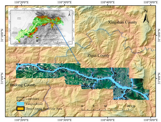
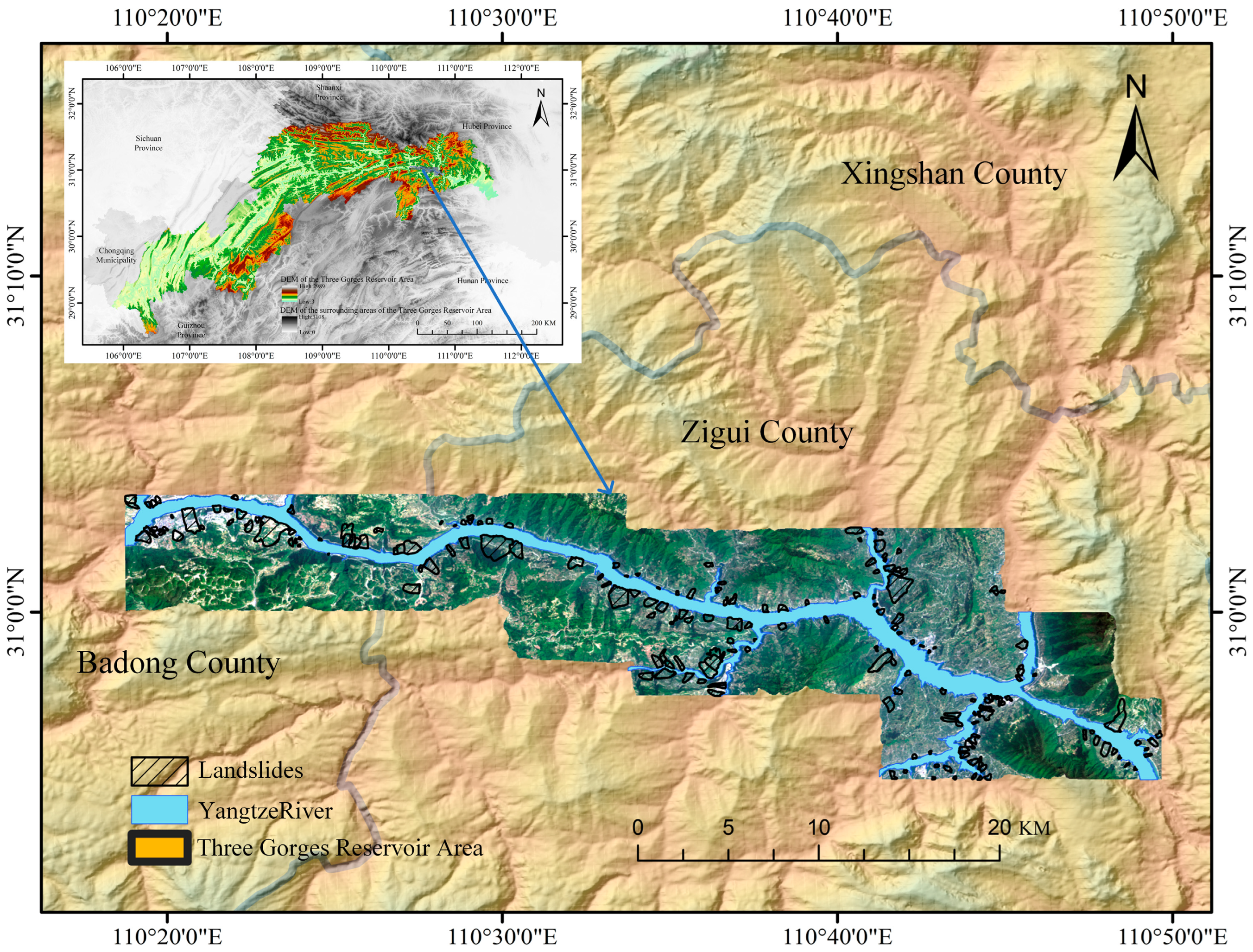
The study area is located in the Zigui–Badong section of the TGRA, characterized by high frequency, diversity, and widespread distribution of geohazards. The primary hazard types include landslides, rockfalls, debris flows, ground fissures, and land subsidence [27]. According to incomplete statistics, over 5000 landslide events have been recorded in the TGRA since 2003 [28].

The study area ranges from 110°18′ E to 110°52′ E and from 30°01′ N to 30°56′ N, as shown in Figure 1. The region is situated in the mid-latitude zone and experiences a subtropical monsoon climate, characterized by distinct seasons, concurrent rainfall and heat, and intense concentrated precipitation with frequent heavy rainstorms, which collectively favor landslide development [29]. Rainfall in the region exhibits distinct seasonality and suddenness, mainly concentrated from May to October, with a high frequency of heavy rainfall events and frequent short-interval multi-peak rainfall patterns [30]. Rainfall infiltration softens rock masses, increases pore water pressure, and triggers landslide hazards, making this area a typical zone with frequent geological disasters in the reservoir area [31].

Figure 1. Overview of the study area.

2.2. Geology and Geomorphology of the Study Area

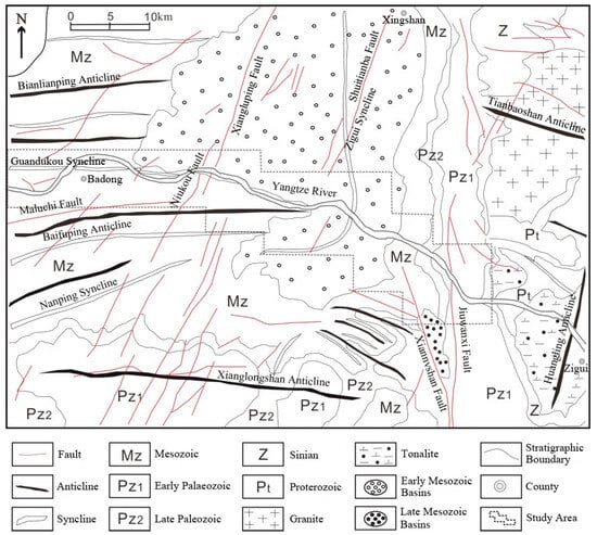
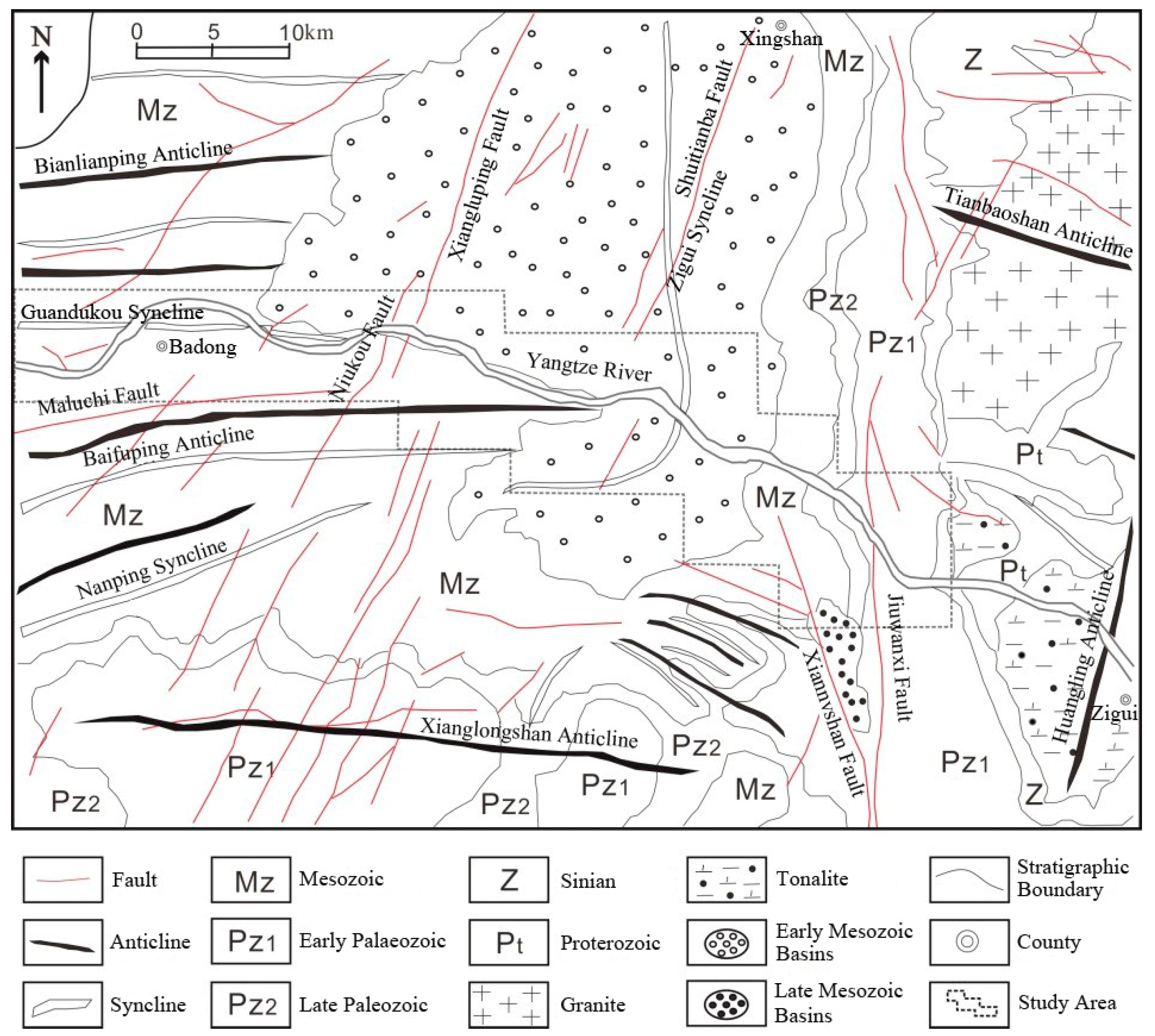
The geological structure of the TGRA belongs to the Neocathaysian structural system, shaped by multiple tectonic movements (e.g., the Jinning and Yanshanian movements), forming a complex structural framework dominated by folds and faults [32]. As a large-scale orogenic movement in the reservoir area, the Yanshanian movement caused extensive intermittent differential uplift of the ground surface, after which crustal movement gradually stabilized [13]. These fold belts and faults have led to frequent occurrences of geological hazards such as landslides and debris flows in the reservoir area. Jurassic and Triassic strata are widely distributed in the Three Gorges Reservoir Area. Jurassic red-bed rock masses are mainly distributed west of Fengjie and east of Zigui, while Triassic red-bed rock masses occur in Badong and Zigui. Limestone, marl, dolomite, and other lithologies are also found in other regions. In terms of lithological characteristics, Jurassic strata have low mechanical strength and weak external resistance, providing favorable conditions for the development of landslides and other geological disasters.

The study area has a complex geological environment and significant topographic relief, with an overall east–west topographic trend of being higher in the west and lower in the east. It is densely covered with mountains, and the river valley areas are relatively narrow. The Yangtze River and its tributaries flow through the region. Badong County features typical karst landforms, and intense human activity—such as road construction and land reclamation—may further exacerbate the occurrence of landslides [33]. A geological map of the study area is shown in Figure 2.

Figure 2. Geological overview of the study area.

2.3. Data Sources

The data sources used in this study are shown in Table 1.

Table 1. Data sources used in this study.

Name	Data Source	Spatial Resolution/Scale
DEM data	https://lpdaac.usgs.gov/tools/data~pool/ (accessed on 16 November 2021)	30 m
Basic geographic data	Hubei Geological Survey Institute (accessed on 10 November 2022)	1:50,000
Basic geological data	Hubei Geological Survey Institute (accessed on 10 October 2023)	1:50,000
Hydrological data	Geospatial Data Cloud http://www.gscloud.cn/	1:50,000
Landslide distribution data	Landslide hazard map (accessed on 12 November 2021)	1:10,000

The data employed in this study primarily include DEM, basic geographic data, basic geological data, hydrological data, and landslide distribution data. The basic geographic, basic geological, and hydrological data are at a scale of 1:50,000, while the landslide data are at a scale of 1:10,000. Both meet the data precision requirements for the 30 m resolution DEM. All datasets were resampled to a unified 30 m × 30 m grid resolution based on the principle of lowest resolution, serving as the evaluation unit for subsequent analysis.

3. Research Methods

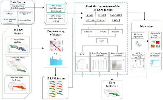
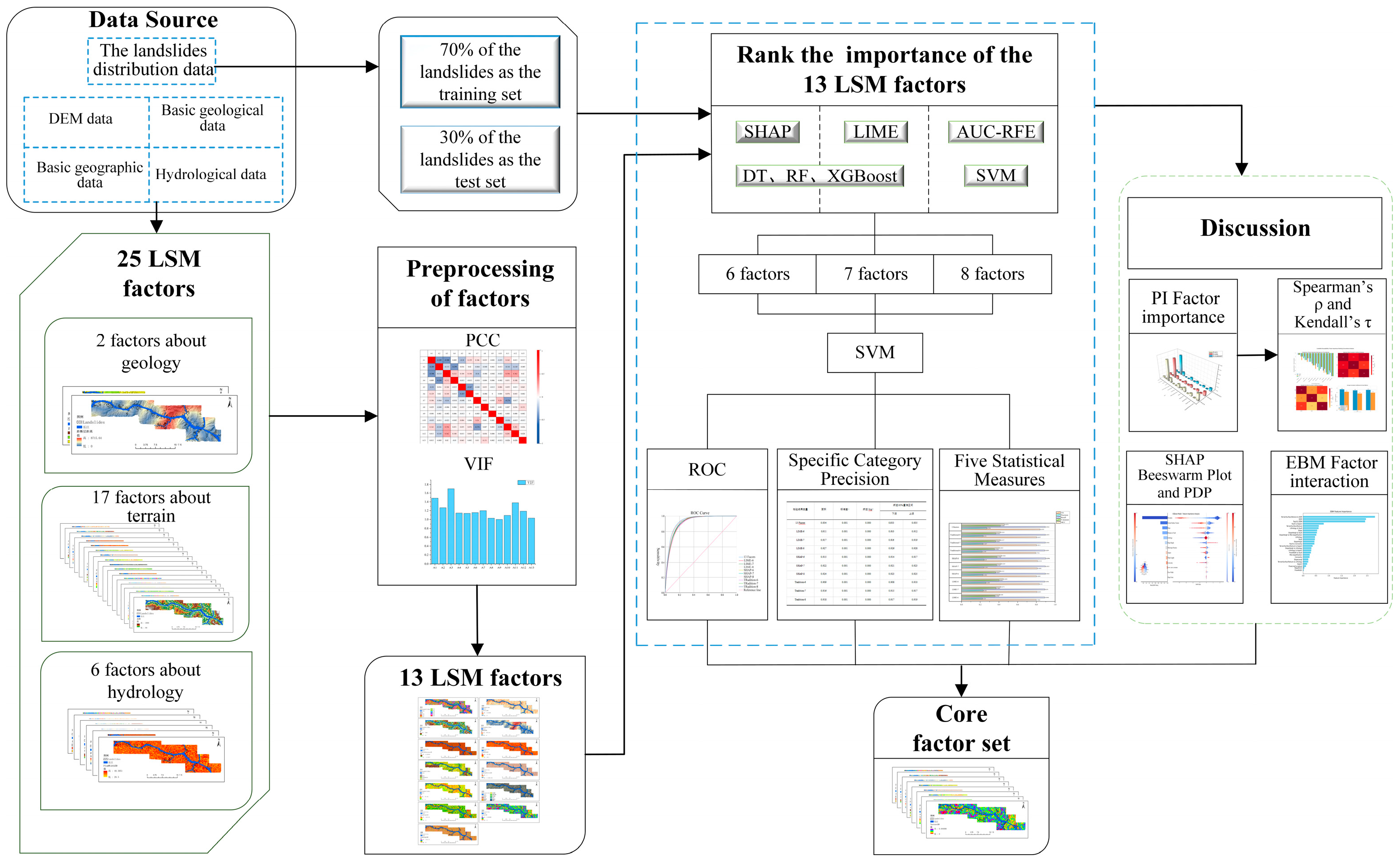
The entire experimental workflow is shown in Figure 3. First, combined with remote sensing images and geological survey data of the study area, 202 landslide locations were identified through expert human–computer interactive interpretation. Second, based on original data such as topographic and geomorphic, geological, and hydrological data as well as remote sensing images of the study area, and referring to previous research results, 25 initial landslide conditioning factors in the study area were generated through calculation. The initial factors were subjected to Pearson’s correlation analysis and multicollinearity diagnostics, resulting in 13 screened factors. For model training, 70% of the landslides (141 events, totaling 19,589 grid cells) were randomly selected, with a 1:1 ratio of landslide to non-landslide samples. The remaining 30% (61 landslides, 6045 grid cells) served as the validation set. The RF, DT, and XGBoost models were then trained and validated. SHAP and LIME were applied separately to interpret the factor importance of these three models, yielding six distinct sets of factor importance rankings. A comprehensive scoring system (1–13 points, from highest to lowest importance) was applied to the results. The scores from the same interpretation model (SHAP or LIME) were averaged to generate two final sets of factor importance rankings. Subsequently, the AUC-RFE method was used to derive a factor ranking, which was then compared with the results from the SHAP and LIME interpretability methods. The top 6–8 factors identified by these approaches were selected for validation and evaluation using the SVM model. Finally, PI and EMB models were employed to analyze factor importance and interaction effects, yielding the final core factor set for the study area.

Figure 3. Experimental workflow.

3.1. Evaluation Models

3.1.1. Random Forest Model

Random Forest (RF) is a machine learning-based ensemble model that trains multiple decision trees on samples and then combines the results of these decision trees to generate the final output. The Random Forest (RF) model is widely applied in landslide susceptibility mapping due to its strong tolerance to noisy data and outliers, and especially its excellent ability to handle large-scale datasets [34]. The mathematical formulation is shown in Equation (1):

$$\mathrm{F}(\mathrm{x})=\mathrm{m}\mathrm{a}\mathrm{x}\left\{{\mathrm{p}}_{\mathrm{i}}={\displaystyle \frac{{\sum }_{\mathrm{j}}^{\mathrm{k}}1{\mathrm{p}}_{\mathrm{i}\mathrm{j}}}{\mathrm{k}}}|\mathrm{i}\in \mathrm{I}\right\}$$

(1)

where F(x) denotes the final prediction probability; k represents the number of decision trees; I is the set of all categories; p_i is the average probability of category i; and p_ij is the prediction result of the j-th decision tree for category i.

3.1.2. Decision Tree Model

A decision tree (DT) is a supervised learning model commonly used for classification and regression tasks. It mainly makes decisions through a tree-like structure, where each internal node of the tree represents a feature-based judgment, and outputs are generated via branches. The leaf nodes correspond to classification categories or values [35]. Decision tree models exhibit strong interpretability, require low data preprocessing effort, and can efficiently process diverse data types.

3.1.3. XGBoost (eXtreme Gradient Boosting)

XGBoost is fundamentally based on the Gradient Boosting Decision Tree (GBDT) algorithm. It combines multiple weak learners (typically decision trees) to form a strong learner, with model accuracy improving as the number of iterations increases [36]. The XGBoost algorithm leverages second-order derivatives obtained via Taylor expansion of the loss function (in addition to first-order derivatives) to accelerate convergence to the optimal solution [37]. Its optimal objective function (Obj(m)) is shown in Equation (2):

$$\mathrm{O}\mathrm{b}{\mathrm{j}}^{\left(\mathrm{m}\right)}=\sum _{\mathrm{i}=1}^{\mathrm{n}}\mathrm{l}\left({\mathrm{y}}_{\mathrm{i}},{\widehat{\mathrm{y}}}_{\mathrm{i}}\right)\sum _{\mathrm{k}=1}^{\mathrm{K}}\Omega \left({\mathrm{f}}_{\mathrm{k}}\right)$$

(2)

where n denotes the number of samples; $\mathrm{l}\left({\mathrm{y}}_{\mathrm{i}},{\widehat{\mathrm{y}}}_{\mathrm{i}}\right)$ is the loss function, which evaluates the error between the predicted value ${\widehat{\mathrm{y}}}_{\mathrm{i}}$ and the true value ${\mathrm{y}}_{\mathrm{i}}$; K represents the number of trees; and $\Omega \left({\mathrm{f}}_{\mathrm{k}}\right)$ is the regularization term of the k-th tree, which controls the model complexity to prevent overfitting.

3.1.4. SVM Model

Support Vector Machine (SVM) is a supervised machine learning model that is frequently used in classification and regression analysis. SVM maps the training data into a high-dimensional space and identifies the optimal n-dimensional hyperplane based on specific rules, thereby maximizing the separation of data into two classes [38]. The fundamental formula of SVM is shown in Equation (3):

$$\left\{\begin{array}{c}\min =\mathrm{L}\left(\omega ,{\mathrm{b}}_0\right)={\displaystyle \frac{1}{2}}{‖\omega ‖}^2 \\ {\mathrm{y}}_{\mathrm{i}}\left({\mathrm{w}}^{\mathrm{T}}{\mathrm{x}}_{\mathrm{i}}+{\mathrm{b}}_0\right)\ge \mathrm{1,2},\dots ,\mathrm{m}.\end{array}\right.$$

(3)

By substituting the Lagrangian formula and KKT conditions into the above, the model Formula (4) of SVM can be derived:

$$\mathrm{f}\left(\mathrm{x}\right)=\sum _{\mathrm{i}=1}^{\mathrm{n}}{\lambda }_{\mathrm{i}}{\mathrm{y}}_{\mathrm{i}}{\mathrm{x}}_{\mathrm{i}}^{\mathrm{T}}\mathrm{x}+\mathrm{b}$$

(4)

where $\omega$ denotes the normal vector of the hyperplane; ${\mathrm{b}}_0$ is the offset of the hyperplane; ${\mathrm{x}}_{\mathrm{i}}$ represents the feature vector of the i-th sample; ${\mathrm{y}}_{\mathrm{i}}$ is the label of the i-th sample, with ${\mathrm{y}}_{\mathrm{i}}\in \left\{1,-1\right\}$; ${\lambda }_{\mathrm{i}}$ is the Lagrange multiplier; and $\mathrm{m}$ is the number of samples.

3.2. Factor Screening Methods

3.2.1. LIME

LIME (Local Interpretable Model-agnostic Explanations) was proposed by Marco et al. in 2016 as a model-agnostic local interpretability algorithm [18]. It was designed to interpret predictions of complex black-box models, addressing the interpretability challenges of complex models [39]. Its mathematical formulation is shown in Equation (5):

$${\mathrm{M}}_{\left(\mathrm{e}\mathrm{x}\mathrm{p}\mathrm{l}\mathrm{a}\mathrm{n}\mathrm{a}\mathrm{t}\mathrm{i}\mathrm{o}\mathrm{n}\right)}(\mathrm{x})={\mathrm{a}\mathrm{r}\mathrm{g}\mathrm{m}\mathrm{i}\mathrm{n}}_{\mathrm{g}}\mathrm{L}(\mathrm{f},\mathrm{g},{\pi }_{\mathrm{x}})+{\Omega }_{(\mathrm{g})}$$

(5)

where L denotes the loss function; g is a simple model for instance x and one of all explanatory models; f represents the original model; ${\Omega }_{(\mathrm{g})}$ is the complexity of the explanatory model g; and ${\pi }_{\mathrm{x}}$ denotes the neighborhood of x.

3.2.2. SHAP

SHAP (SHapley Additive exPlanations) was proposed by Lundberg and Lee in 2017. SHAP values are based on the Shapley value concept from cooperative game theory. Due to their strong interpretability, they are widely used to explain black-box machine learning models, effectively enhancing the credibility of model predictions [40]. The SHAP algorithm calculates the contribution value of each feature in the training data to the prediction results, directly reflecting the influence and weight of the corresponding features in the model’s prediction process [41]. The SHAP value (ϕi) for the (i)-th feature in sample x is calculated as shown in Equation (6):

$${\mathrm{\varnothing }}_{\mathrm{i}}=\sum _{\mathrm{S}\subseteq \mathrm{F}\setminus \left\{\mathrm{i}\right\}}{\displaystyle \frac{\left|\mathrm{S}\right|!\left(\left|\mathrm{F}\right|-\left|\mathrm{S}\right|-1\right)!}{\left|\mathrm{F}\right|!}}\left[{\mathrm{f}}_{\mathrm{x}}\left(\mathrm{S}\cup \left\{\mathrm{i}\right\}\right)-{\mathrm{f}}_{\mathrm{x}}\left(\mathrm{S}\right)\right]$$

(6)

where F denotes the set of all features; S is any subset of the feature set F that does not contain feature i; ∣S∣ represents the number of features in subset S; ${\displaystyle \frac{\left|\mathrm{S}\right|!\left(\left|\mathrm{F}\right|-\left|\mathrm{S}\right|-1\right)!}{\left|\mathrm{F}\right|!}}$ is the weight of different subsets S; and ${\mathrm{f}}_{\mathrm{x}}\left(\mathrm{S}\cup \left\{\mathrm{i}\right\}\right)-{\mathrm{f}}_{\mathrm{x}}\left(\mathrm{S}\right)$ denotes the contribution of the i-th feature to the model’s prediction under subset S.

3.2.3. The Traditional AUC-Based Recursive Feature Elimination (AUC-RFE)

Feature Recursive Elimination (RFE) is a method that iteratively constructs susceptibility models and uses model performance improvement or decline as an evaluation metric. In each iteration, it removes the least or most important feature based on the results, then repeats the process with the remaining features until all features are eliminated, ultimately generating a feature importance ranking [42]. Building upon this foundation, this study uses the AUC value as the model performance metric and constructs an AUC-based Recursive Feature Elimination (AUC-RFE) method. In this study, the SVM model was selected to construct the susceptibility model, with the AUC value serving as the evaluation metric. The factor that caused the largest reduction in AUC was removed in each iteration. The specific steps are as follows:

(1) In the selected factor combination, sequentially remove each factor and record the corresponding AUC value.

(2) Eliminate the factor causing the largest AUC drop.

(3) Use the remaining factors as the initial set for the next iteration, and repeat steps (1) and (2) until all factors are removed.

Therefore, in the AUC-RFE method, the earlier a factor is removed, the more important it is. The importance of factors is ranked according to the order of their removal.

3.3. Factor Correlation Analysis Methods

3.3.1. Pearson’s Correlation Coefficient

The Pearson correlation coefficient (PCC) is used to analyze the correlation between selected factors, screening out and eliminating factors with excessively strong correlations. This effectively reduces the impact of inter-factor correlations on the prediction accuracy of the model [43]. Generally, when PCC ≤ 0.5, it indicates no significant correlation between factors [44].

3.3.2. Multicollinearity

Multicollinearity refers to the linear correlation phenomenon among independent variables. Typically, the Variance Inflation Factor (VIF) is used to analyze multicollinearity between factors [45]. When VIF < 10, it indicates no significant multicollinearity between the factors.

3.4. Result Evaluation Methods

3.4.1. Receiver Operating Characteristic and Area Under the Curve

The Receiver Operating Characteristic (ROC) curve is a commonly used evaluation tool for classification models, offering an intuitive representation of model performance [46]. It plots the True Positive Rate (TPR) on the y-axis and the False Positive Rate (FPR) on the x-axis, as shown in Equations (7) and (8). The Area Ander the Curve (AUC) is a common metric for evaluating the performance of an ROC curve. The AUC value typically ranges between 0.5 and 1. A higher AUC indicates better model performance, while an AUC value below 0.5 suggests that the experiment is ineffective.

$$\mathrm{T}\mathrm{P}\mathrm{R}={\displaystyle \frac{\mathrm{T}\mathrm{P}}{\mathrm{T}\mathrm{P}+\mathrm{F}\mathrm{N}}}$$

(7)

$$\mathrm{F}\mathrm{P}\mathrm{R}={\displaystyle \frac{\mathrm{F}\mathrm{P}}{\mathrm{F}\mathrm{P}+\mathrm{T}\mathrm{N}}}$$

(8)

3.4.2. Specific Category Precision Analysis

Specific category precision analysis is a method used to evaluate the performance of a classification model on specific categories. It is widely applied in landslide susceptibility mapping, enabling quantitative analysis of experimental results based on different susceptibility levels [47], as shown in Equation (9):

$${\mathrm{P}}_{\mathrm{i}}={\displaystyle \frac{{\mathrm{A}}_{\mathrm{i}}}{{\mathrm{B}}_{\mathrm{i}}}}\times 100\%$$

(9)

where i is the number of classes in the landslide susceptibility zoning; Ai is the number of landslides in the i-th class of the landslide susceptibility zoning; Bi is the total number of samples in the i-th class of the landslide susceptibility zoning; Pi is the class-specific accuracy of the i-th class of the landslide susceptibility zoning.

3.4.3. Five Statistical Measures

In landslide susceptibility mapping, five commonly used statistical measures for evaluating classification models based on the confusion matrix are Overall Accuracy (OA), precision, recall, F-measure, and the Matthews Correlation Coefficient (MCC). OA reflects the model’s overall prediction accuracy across the study area, where a higher OA value indicates more accurate landslide predictions. Precision refers to the regions predicted as landslides by the model within the study area, where a higher precision value indicates a higher proportion of actual landslide occurrences among the areas classified as landslides by the model. Recall focuses on landslides that have actually occurred; a higher recall value indicates a larger proportion of real landslide areas successfully identified as landslides by the model. The F-measure integrates precision and recall through a weighted harmonic mean, with higher values representing stronger overall effectiveness. The MCC comprehensively reflects the correlation between predicted results and actual conditions: an MCC value of 1 indicates perfect alignment between predictions and reality; a value of 0 means the predictions are no better than random guessing; and a value of −1 represents complete inconsistency between predictions and reality [48,49]. The formulas for these five methods are shown in Equations (10)–(14):

$$\mathrm{O}\mathrm{A}={\displaystyle \frac{\mathrm{T}\mathrm{P}+\mathrm{T}\mathrm{N}}{\mathrm{T}\mathrm{P}+\mathrm{F}\mathrm{P}+\mathrm{T}\mathrm{N}+\mathrm{T}\mathrm{P}}}$$

(10)

$$\mathrm{P}\mathrm{r}\mathrm{e}\mathrm{c}\mathrm{i}\mathrm{s}\mathrm{i}\mathrm{o}\mathrm{n}={\displaystyle \frac{\mathrm{TP}}{\mathrm{TP}+\mathrm{FP}}}$$

(11)

$$\mathrm{R}\mathrm{e}\mathrm{c}\mathrm{a}\mathrm{l}\mathrm{l}={\displaystyle \frac{\mathrm{T}\mathrm{P}}{\mathrm{T}\mathrm{P}+\mathrm{F}\mathrm{N}}}$$

(12)

$$\mathrm{F}-\mathrm{m}\mathrm{e}\mathrm{a}\mathrm{s}\mathrm{u}\mathrm{r}\mathrm{e}={\displaystyle \frac{2 \times \mathrm{Precision} \times \mathrm{Recall}}{\mathrm{P}\mathrm{r}\mathrm{e}\mathrm{c}\mathrm{i}\mathrm{s}\mathrm{i}\mathrm{o}\mathrm{n}+\mathrm{R}\mathrm{e}\mathrm{c}\mathrm{a}\mathrm{l}\mathrm{l}}}$$

(13)

$$\mathrm{M}\mathrm{C}\mathrm{C}={\displaystyle \frac{\mathrm{T}\mathrm{P}\times \mathrm{T}\mathrm{N}-\mathrm{F}\mathrm{P}\times \mathrm{F}\mathrm{N}}{\sqrt{\left(\mathrm{T}\mathrm{P}+\mathrm{F}\mathrm{P}\right)\left(\mathrm{T}\mathrm{P}+\mathrm{F}\mathrm{N}\right)\left(\mathrm{T}\mathrm{N}+\mathrm{F}\mathrm{P}\right)\left(\mathrm{T}\mathrm{N}+\mathrm{F}\mathrm{N}\right)}}}$$

(14)

4. Results and Analysis of Landslide Susceptibility Mapping

4.1. Factor Correlation Results

Based on the characteristics of the study area and previous research findings, this study selected 25 factors influencing landslides within the research area [50], as shown in Table 2.

Table 2. Overview of factors.

Type	Variable	Unit	Value Range
Geology	Distance to Fault	m	0~8715.64
	Lithology		1. hard rock; 2. soft–hard alternating rock; 3. soft rock.
Terrain	Elevation	m	80~2000
	ValleyDept	m	0.00256774~1308.15
	TPI		−83.3541~227.751
	Terrain Surface Texture		0~0.694006
	Tangential Curvature		−0.0749825~0.0468265
	Slope Length	m	0~4137.74
	Slope Height	m	0~1227.48
	Slope Form		1. Outside Convex Slope; 2. Outside Concave Slope; 3. Outside Straight Slope; 4. Inside Convex Slope; 5. Inside Concave Slope; 6. Inside Straight Slope; 7. Straight Convex Slope; 8. Straight Concave Slope; 9. Straight Slope.
	Slope		0~78.419
	Profile Curvature		−0.0689291~0.0629155
	Plan Curvature		−1.96555~4.0909
	Minimal Curvature		−0.405303~0.0755154
	Mid-slope Position		0~1
	Longitudinal Curvature		−0.639569~0.242719
	Landforms		1. Canyons, deeply incised streams; 2. mid-slope drainages, shallow valleys; 3. upland drainages, headwaters; 4. U-shape valleys; 5. plains; 6. open slopes; 7. upper slopes, mesas; 8. local ridges/hills in valleys; 9. mid-slope ridges, small hills in plains; 10. mountain tops, high ridges.
	Convexity		0~0.81388
	Aspect		−1. Plane; 1. North; 2. Northeast; 3. East; 4. Southeast; 5. South; 6. Southwest; 7. West; 8. Northwest
Hydrology	VDCN	m	−464.027~1724.15
	SPI		0~1136150
	MRN		0~37.728
	Flow Width	m	28.5~40.3051

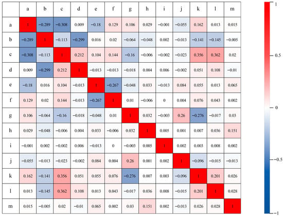
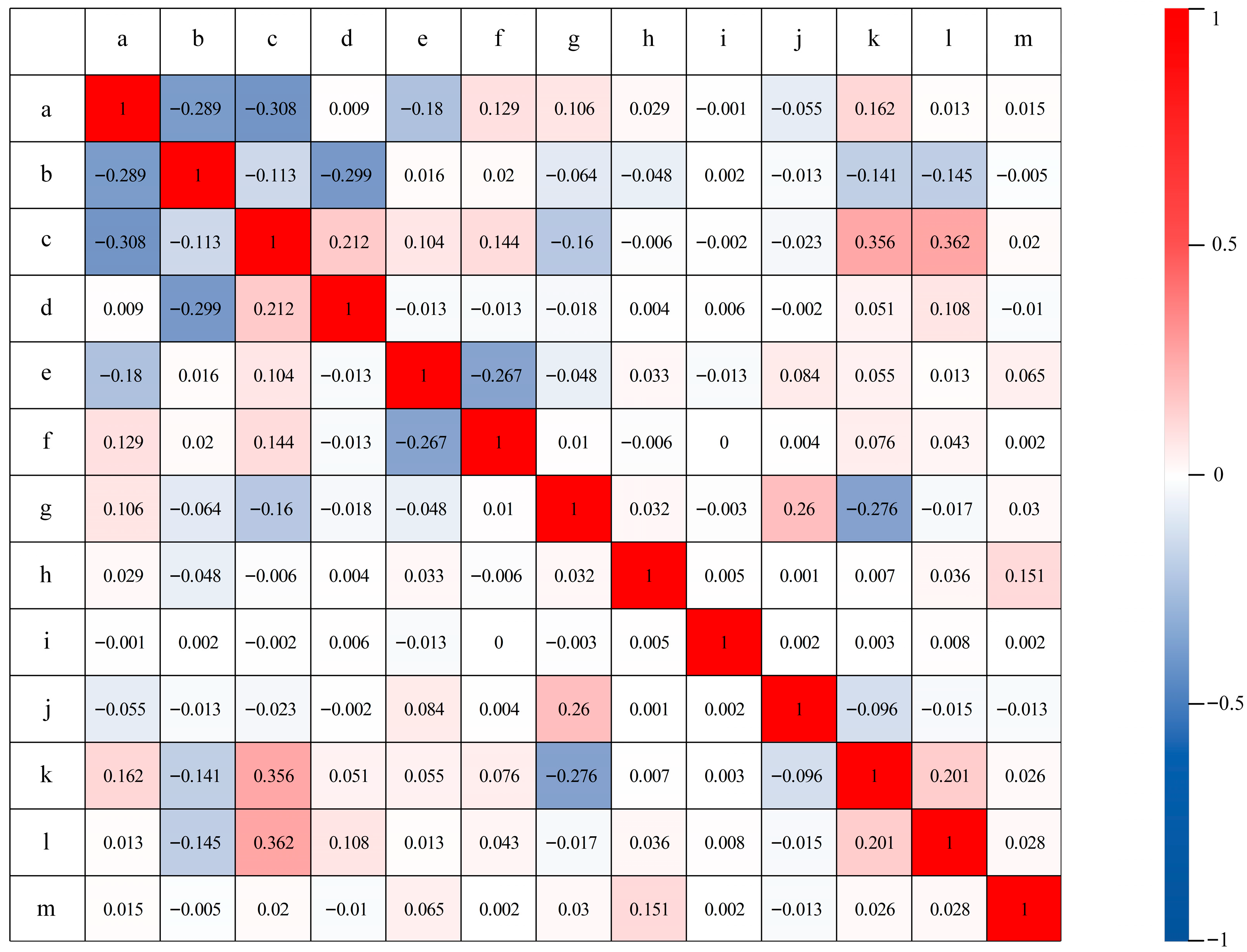
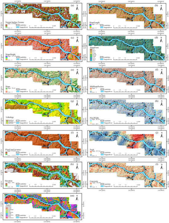
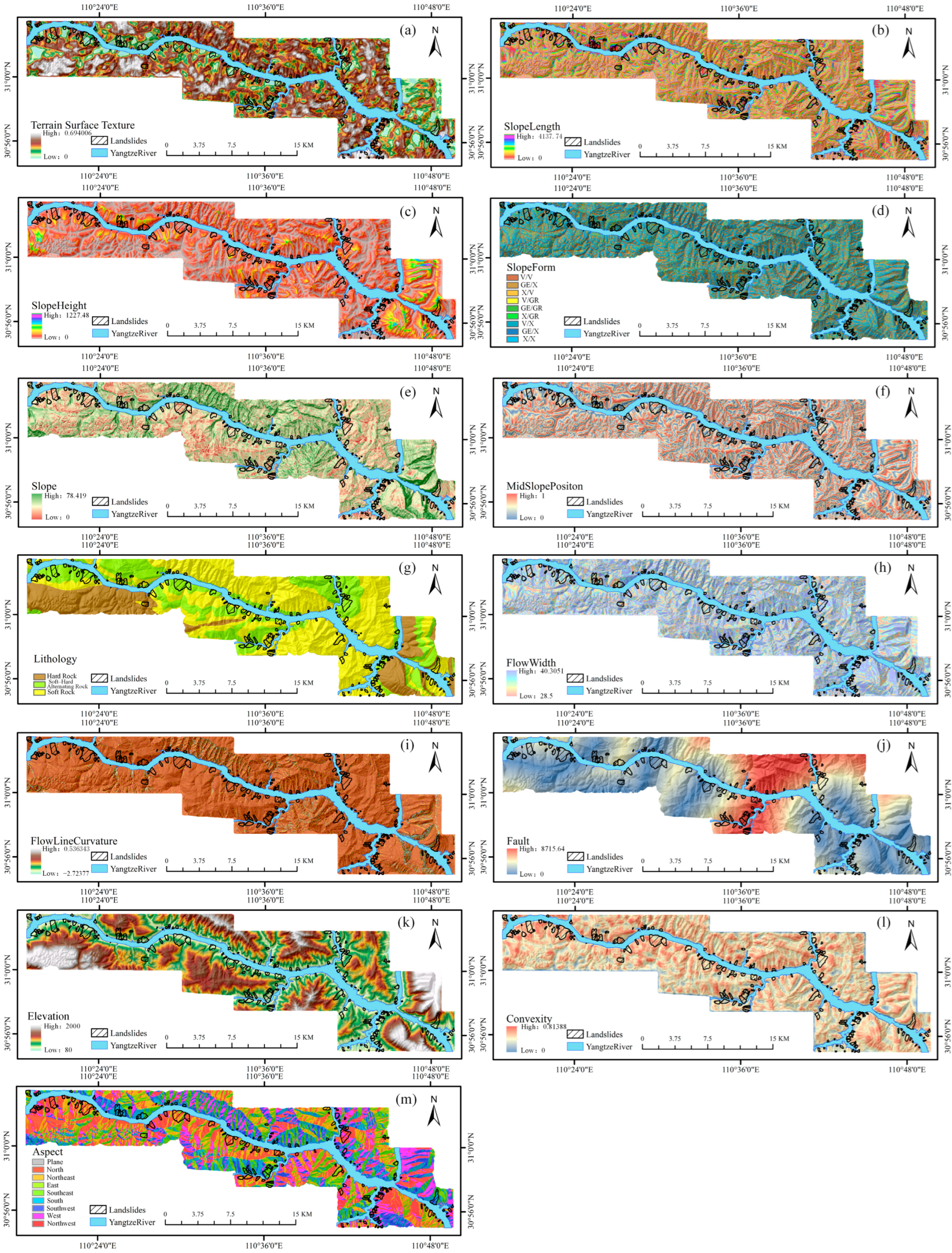
The selected factors were screened using PCC and multicollinearity analysis. Factors with a PCC value greater than 0.5 and a Variance Inflation Factor (VIF) greater than 10 were excluded. Finally, a total of 13 factors were retained for modeling, including Terrain Surface Texture, Slope Length, Slope Height, Slope Form, Slope, Mid-slope Position, Lithology, Flow Width, Flow Line Curvature, Distance to Fault, Elevation, Convexity, and Aspect. The PCC and VIF values of the screened factors are shown in Figure 4 and Table 3, respectively, and the overview diagrams of each factor are shown in Figure 5.

Figure 4. PCC values of the screened factors (a. Terrain Surface Texture, b. Slope Length, c. Slope Height, d. Slope Form, e. Slope, f. Mid-slope Position, g. Lithology, h. Flow Width, i. Flow Line Curvature, j. Distance to Fault, k. Elevation, l. Convexity, m. Aspect).

Table 3. VIF values of the screened factors.

Factors	TOL	VIF
Terrain Surface Texture	0.674	1.483
Slope Length	0.790	1.266
Slope Height	0.586	1.707
Slope Form	0.872	1.146
Slope	0.878	1.138
Mid-slope Position	0.865	1.156
Lithology	0.972	1.028
Flow Width	0.834	1.199
Flow Line Curvature	1.000	1.000
Distance to Fault	0.916	1.092
Elevation	0.725	1.379
Convexity	0.842	1.087
Aspect	0.970	1.131

Figure 5. Overview of Factors ((a) Terrain Surface Texture; (b) Slope Length; (c) Slope Height; (d) Slope Form; (e) Slope; (f) Mid-slope Position; (g) Lithology; (h) Flow Width; (i) Flow Line Curvature; (j) Distance to Fault; (k) Elevation; (l) Convexity; (m) Aspect).

4.2. Establishment of Training and Validation Datasets

The study area consists of a total of 405,967 raster cells, with 202 landslides recorded. The landslide inventory was validated using FAD, with a minimum landslide area of 2068.8 m² in the study area. The data follows a power-law distribution (α = 2.192), consistent with typical landslide statistical characteristics [51]. To reduce the impact of spatial autocorrelation in the study area on model training and evaluation, the spatial isolation sampling method under buffer constraints was adopted: a 150 m buffer zone was set around each landslide area during sampling to avoid inaccuracies in landslide boundary delineation; non-landslide samples were selected using a 3 × 3 grid window to eliminate spatial aggregation of non-landslide samples, thus ensuring spatial independence between the training set and the validation set [52]. On this basis, 70% of the landslides, namely, 141 landslide sites (corresponding to 19,589 raster cells in total), were randomly selected; a training set was constructed following a 1:1 ratio of landslide to non-landslide samples, and the remaining 30% of the landslides (61 landslide sites, corresponding to 6045 raster cells in total) were used as the validation set.

4.3. Factor Importance Results

4.3.1. Interpretability Results of Machine Learning Models

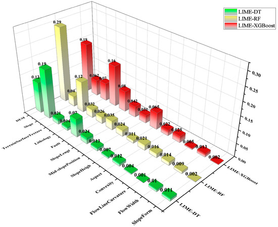
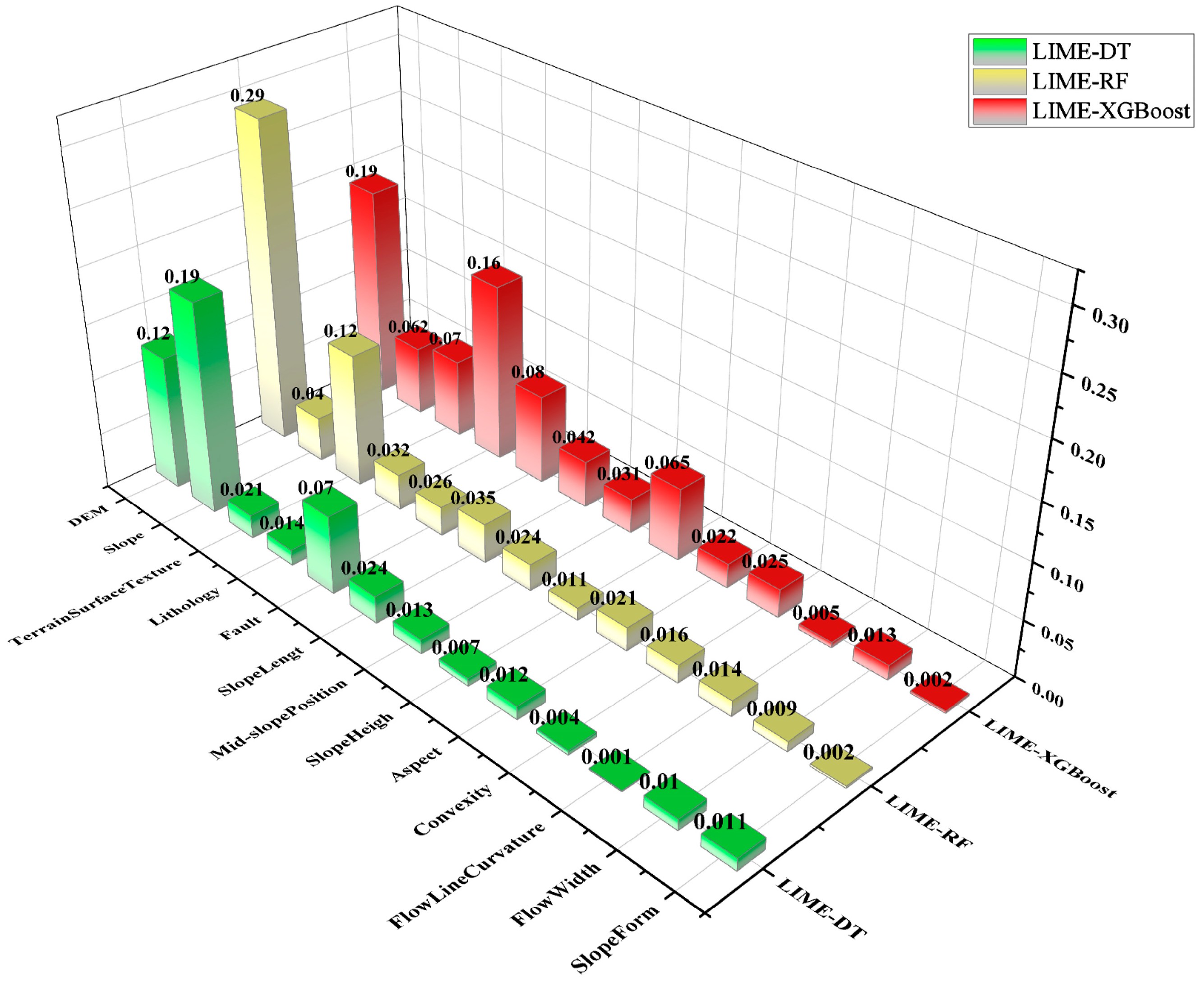
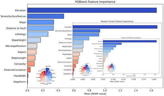
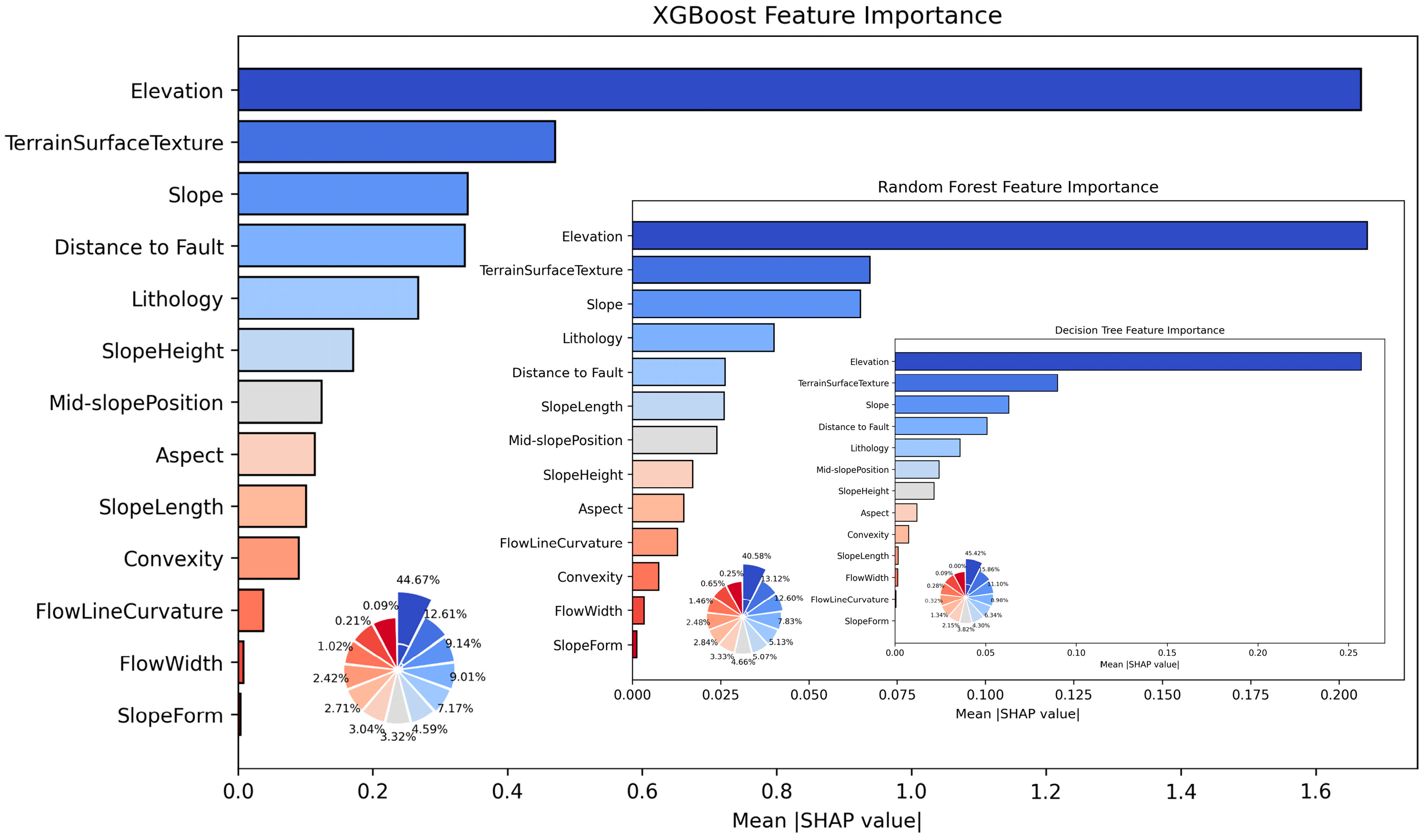
The training set was input into RF, DT, and XGBoost models for training. The trained models and their predictions were then interpreted using LIME and SHAP, yielding six sets of factor importance results (as shown in Figure 6 and Figure 7). Each set of factor importance results was ranked from high to low and scored sequentially from 1 to 13. The scores were averaged according to the interpretability method (LIME or SHAP) to generate two comprehensive factor ranking results, as shown in Table 4.

Figure 6. LIME factor importance diagram.

Figure 7. SHAP factor importance diagram.

Table 4. Ranking results of factor importance based on LIME and SHAP.

Ranking	LIME	SHAP
1	Elevation	Elevation
2	Slope	Terrain Surface Texture
3	Lithology	Slope
4	Terrain Surface Texture	Distance to Fault
5	Distance to Fault	Lithology
6	Slope Length	Mid-slope Position
7	Mid-slope Position	Slope Height
8	Aspect	Slope Length
9	Slope Height	Aspect
10	Flow Width	Convexity
11	Convexity	Flow Line Curvature
12	Flow Line Curvature	Flow Width
13	Slope Form	Slope Form

From Table 4, it can be observed that both LIME and SHAP methods consistently identify Elevation as the most important factor and Slope Form as the least important. Furthermore, by comparing the sets of the top six, top seven, and top eight factors ranked by the two methods, it is found that there is only one differing factor in each set. For instance, among the top six factors, five are shared: Elevation, Terrain Surface Texture, Slope, Distance to Fault, and Lithology; the difference lies in that the sixth factor in SHAP is Mid-slope Position, while that in LIME is Slope Length. Among the top seven factors, the first six factors—Elevation, Terrain Surface Texture, Slope, Distance to Fault, Lithology, and Mid-slope Position—are consistent between the two methods, with the differing factors being Slope Height (in SHAP) and Slope Length (in LIME). For the top eight factors, the divergent factors are Aspect and Slope Height, and each of these two factors ranks ninth in the other interpretability method.

4.3.2. Results of AUC-RFE

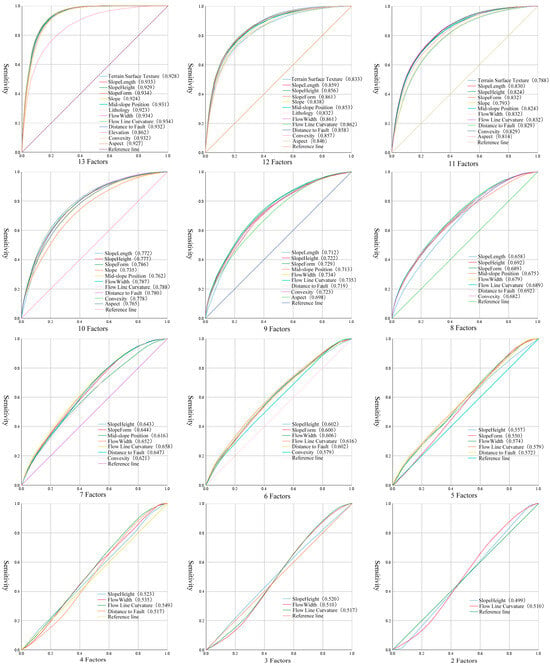
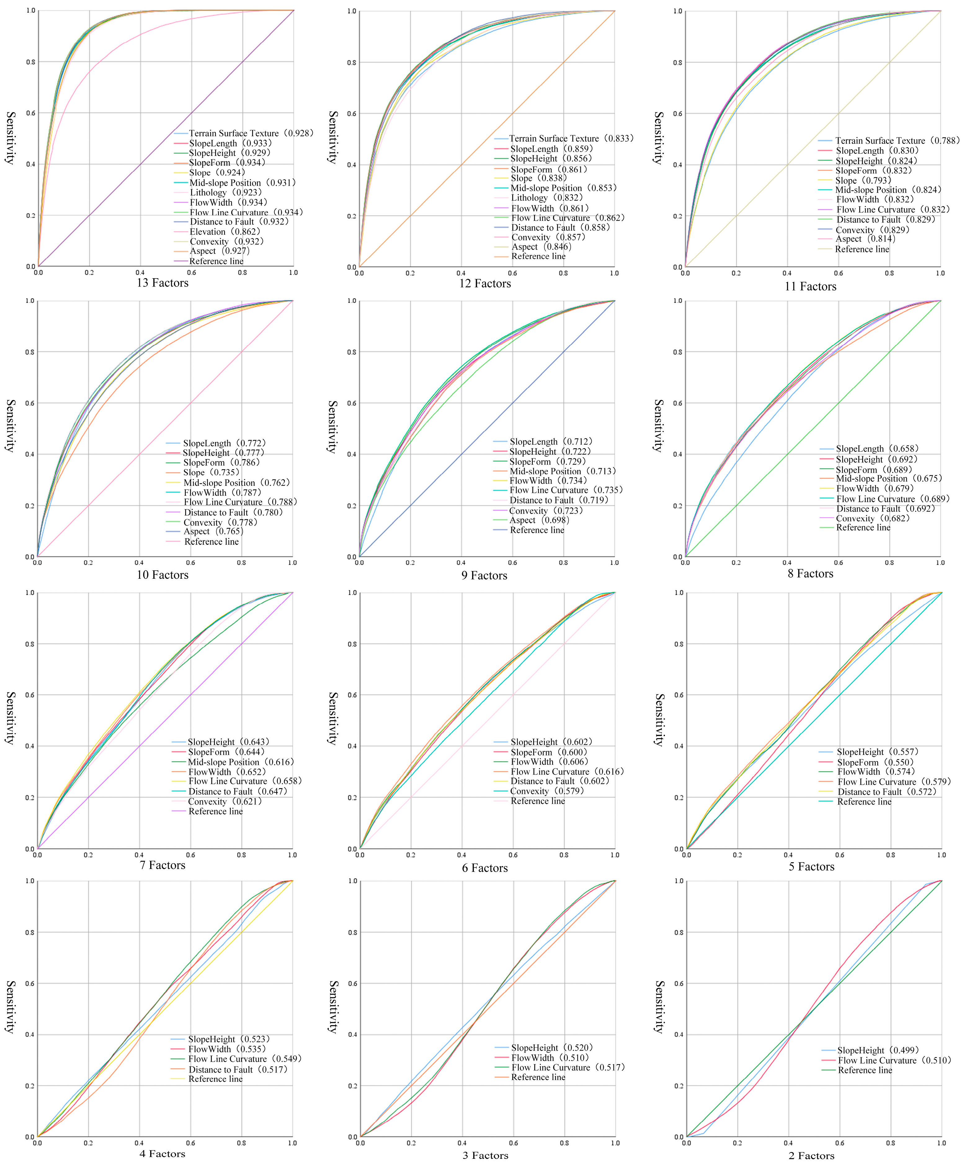
The same training set mentioned above was input into the SVM model for screening, and 13 sets of experiments were conducted with one factor removed each time. Following the method described in Section 3.2.3, the ROC curves and AUC values of the experimental results from AUC-RFE are shown in Figure 8 and Table 5.

Figure 8. AUC-RFE experimental result plots (each group named after the single removed factor).

Table 5. AUC values of each AUC-RFE experimental group.

	Experimental Group	13 Factors	12 Factors	11 Factors	10 Factors	9 Factors	8 Factors	7 Factors	6 Factors	5 Factors	4 Factors	3 Factors	2 Factors
Removed Factor (Ranking)
Elevation		0.862
Lithology		0.923	0.832
Terrain Surface Texture		0.928	0.833	0.788
Slope		0.924	0.838	0.793	0.735
Aspect		0.927	0.846	0.814	0.765	0.698
Slope Length		0.933	0.859	0.830	0.772	0.712	0.658
Mid-slope Position		0.931	0.853	0.824	0.762	0.713	0.675	0.616
Convexity		0.932	0.857	0.829	0.778	0.732	0.682	0.621	0.579
Slope Form		0.934	0.861	0.832	0.786	0.729	0.689	0.644	0.600	0.550
Distance to Fault		0.932	0.858	0.829	0.780	0.719	0.692	0.647	0.602	0.572	0.517
Flow Width		0.934	0.861	0.832	0.787	0.734	0.697	0.652	0.606	0.574	0.535	0.510
Slope Height		0.929	0.856	0.824	0.777	0.722	0.692	0.643	0.602	0.557	0.523	0.520	0.499
Flow Line Curvature		0.934	0.862	0.832	0.788	0.735	0.698	0.658	0.616	0.579	0.549	0.517	0.510

As shown in Figure 8 and Table 5, the factors were ranked according to the order in which they were sequentially removed, and the factor importance results are as follows: Elevation, Lithology, Terrain Surface Texture, Slope, Aspect, Slope Length, Mid-slope Position, Convexity, Slope Form, Distance to Fault, Flow Width, Slope Height, Flow Line Curvature.

4.4. ROC Curves and AUC Values

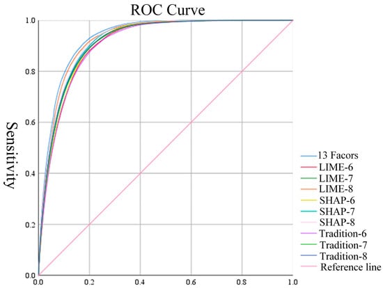
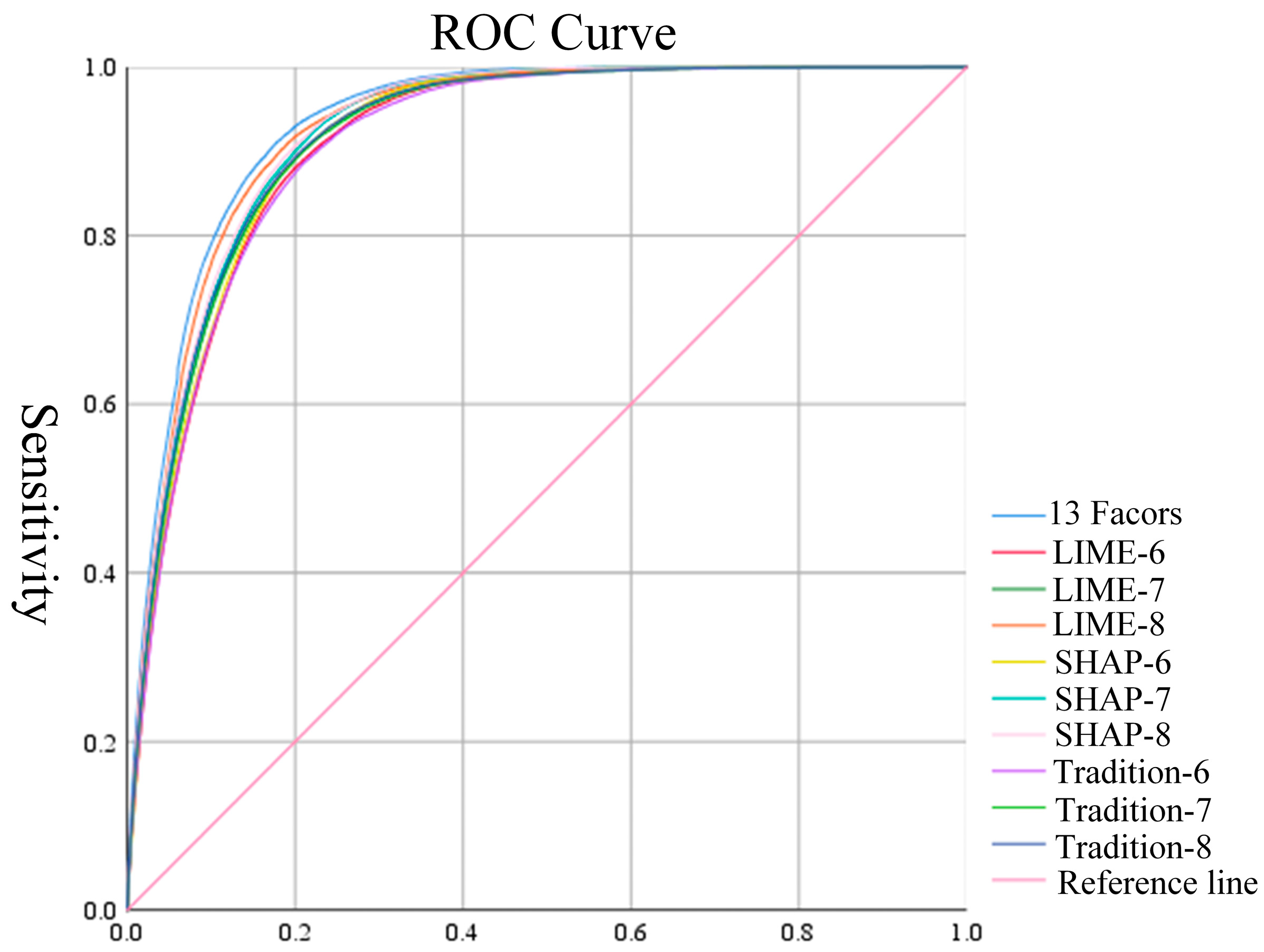
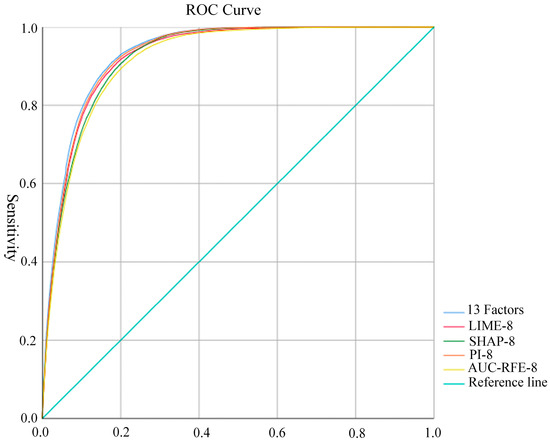
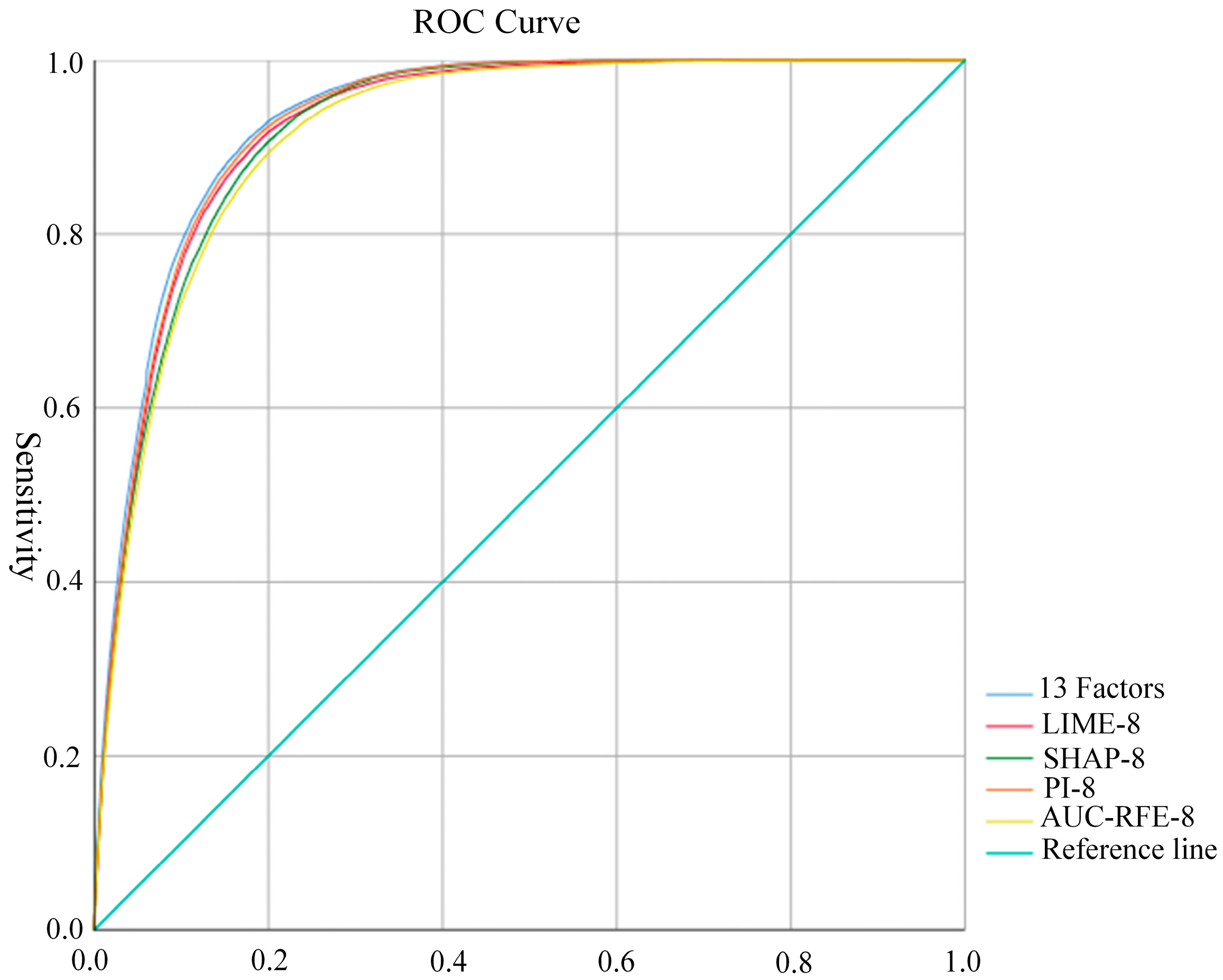
This study conducted a horizontal comparison of the factor importance rankings derived from the three methods mentioned above, while also comparing them with the results based on all 13 screened factors. SVM was selected as the validation model owing to its excellent generalization under limited labeled samples in the study area [53,54], with experiments performed using the top six, seven, and eight factors from each method [55,56,57]. The experimental results were analyzed using the evaluation methods described in Section 3.4.1. The results were evaluated using ROC curves, as shown in Figure 9. To facilitate comparison of outcomes under different conditions for the same model, the AUC values were typically selected, as shown in Table 6.

Figure 9. ROC curves.

Table 6. Area under the curve (AUC) analysis.

Statistical Test Results	Area	Standard Deviation a	Asymptotic Sig. b	Asymptotic 95% Confidence Interval
				Lower Bound	Upper Bound
13 Factors	0.934	0.001	0.000	0.933	0.935
LIME-6	0.911	0.001	0.000	0.910	0.912
LIME-7	0.917	0.001	0.000	0.916	0.919
LIME-8	0.927	0.001	0.000	0.926	0.928
SHAP-6	0.915	0.001	0.000	0.914	0.917
SHAP-7	0.922	0.001	0.000	0.921	0.923
SHAP-8	0.924	0.001	0.000	0.923	0.925
AUC-RFE-6	0.909	0.001	0.000	0.908	0.910
AUC-RFE-7	0.916	0.001	0.000	0.915	0.917
AUC-RFE-8	0.918	0.001	0.000	0.917	0.919

Note: a. under the non-parametric assumption; b. null hypothesis: actual area = 0.5.

As can be observed from Figure 9 and Table 6, with the gradual increase in the number of selected factors, the AUC values of each screening method also increase. When the top six or seven factors were used for experiments, the factors screened by SHAP yielded the highest AUC values (0.915 and 0.922), while those from AUC-RFE were the lowest (0.909 and 0.916). However, when the top eight factors were selected as the core factor set, the AUC value of the factors screened by LIME (0.927) was higher than that of SHAP and AUC-RFE (0.924 and 0.918). Furthermore, the results of these two machine learning interpretability methods showed no significant difference from those obtained using 13 screened factors (0.934), with all AUC values exceeding 0.9. This indicates that both methods are effective.

5. Discussion

As can be observed from the aforementioned experimental results, the factor combinations screened by the two machine learning interpretability methods demonstrate similar performance across all evaluation metrics compared to those derived from all 13 screened factors, and outperform the factor selection results of the AUC-RFE method. However, there are certain discrepancies in the factor importance rankings generated by the two methods, failing to achieve complete consistency. Among the top eight ranked factors, seven are identical: Elevation, Slope, Lithology, Terrain Surface Texture, Distance to Fault, Slope Length, and Mid-slope Position. The difference lies in the eighth factor—specifically, the eighth factor in both SHAP-8 and LIME-8 corresponds to the ninth most important factor in the other method.

To more accurately and scientifically identify the core factor set for landslides in the study area, in this chapter, two additional machine learning interpretability methods—PI and EBM—are incorporated into the study. The interpretability of PI is utilized to re-rank the factors, while the interaction capability of EBM is employed to quantify the importance of interactions between factors. Finally, the overall results are validated and discussed comprehensively.

5.1. Core Factor Set Screening Analysis

5.1.1. PI Factor Importance Results

Permutation Importance (PI), also known as Permutation Feature Importance, is a commonly used model-agnostic method for evaluating feature importance in machine learning. It quantifies the contribution of each feature to model predictions, thereby aiding understanding of the behavior of black-box models [58].

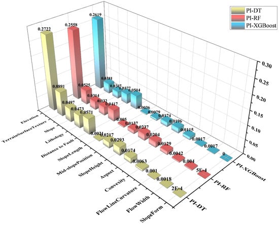
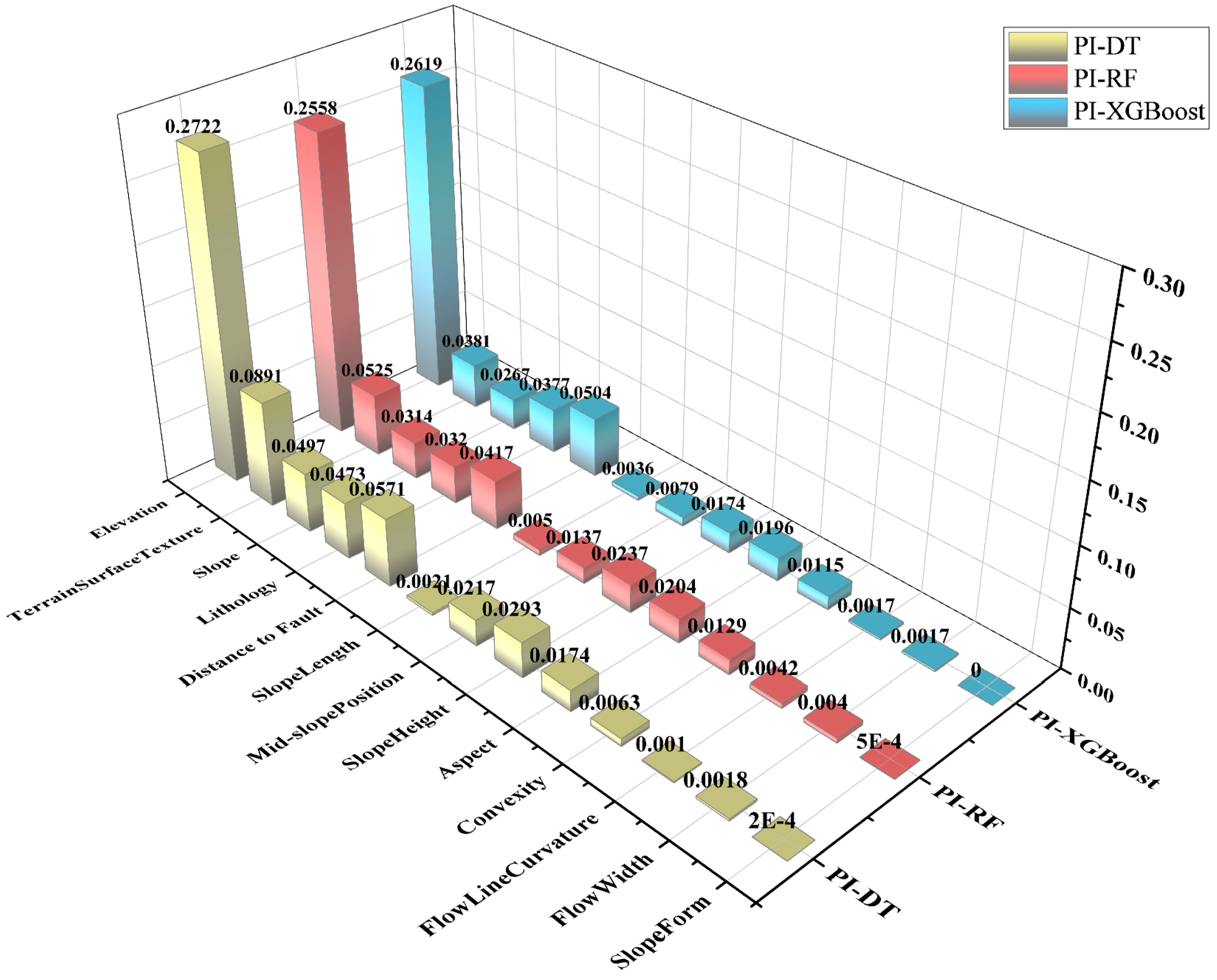
Experiments were conducted using the training set constructed and selected in Section 4.2, along with the evaluated models. The trained models were then interpreted using the Permutation Importance (PI) method, resulting in three distinct sets of factor importance results, as shown in Figure 10.

Figure 10. PI factor importance results.

Using the same method described in Section 4.3.1, the results from Figure 10 were scored to derive the factor importance rankings screened by the PI. The factor importance ranking of the PI in descending order is as follows: Elevation, Terrain Surface Texture, Distance to Fault, Slope, Lithology, Slope Height, Mid-slope Position, Aspect, Convexity, Slope Length, Flow Width, Flow Line Curvature, and Slope Form.

5.1.2. Consistency Verification of Results from Machine Learning Interpretability Methods

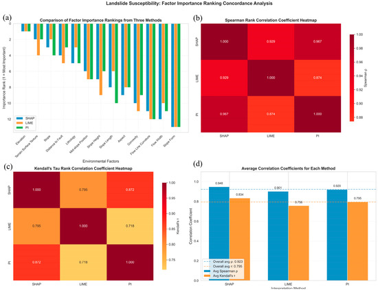
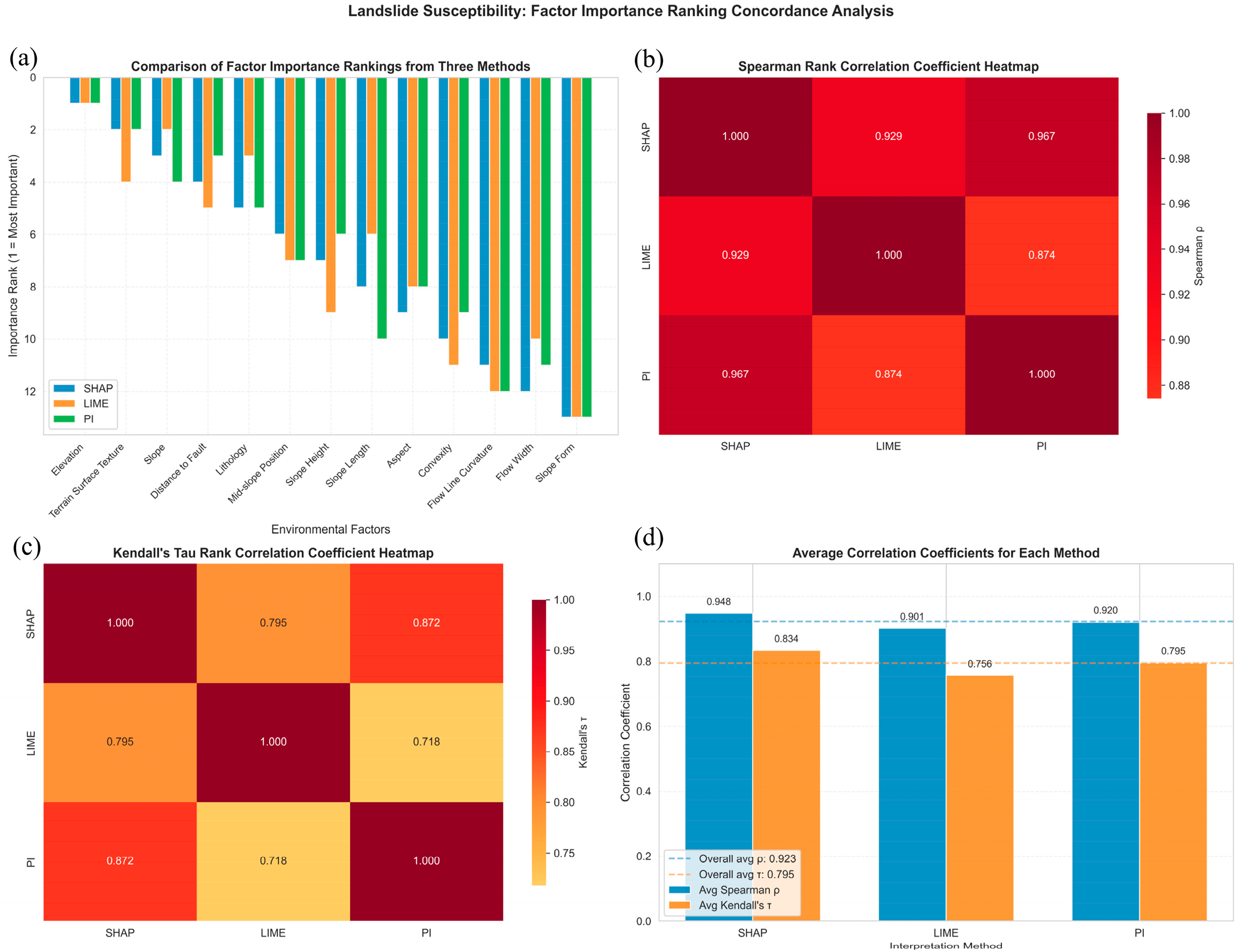
Both Spearman’s rank correlation coefficient (Spearman’s ρ) and Kendall’s tau coefficient (τ) are non-parametric statistical indices, with their value ranges both falling within [−1, 1]. Spearman’s ρ measures the monotonic correlation between two ranked variables by calculating the squared differences of their ranks. Kendall’s τ can be used to quantify the direct consistency between two ranking results. Both methods can effectively verify the reliability of the factor ranking results [59]. The factor importance results derived from LIME, SHAP and PI, along with the corresponding Spearman’s ρ and Kendall’s τ values, are shown in Figure 11.

Figure 11. Consistency analysis of results ((a) factor importance ranking from three methods; (b) Spearman’s ρ Heatmap; (c) Kendall’s τ Heatmap; (d) average correlation coefficients for each method).

It can be observed from Figure 11b–d that the ρ values between each pair of methods are all above 0.9, and the τ values are all above 0.75, indicating a high level of consistency and high similarity of results among these methods. Therefore, it is only necessary to discuss the discrepant factors among the methods. According to the results of the three methods presented in Figure 11a, six factors are shared among the top eight factors, namely, DEM, Terrain Surface Texture, Slope, Fault, Lithology and Mid-slope Position, while the discrepant ones are Slope Height, Slope Length, and Aspect.

To further clarify the importance of these three distinct factors, the factors were grouped in pairwise combinations, which are identical to the factor combinations of the aforementioned experimental groups (SHAP-8, LIME-8, and PI-8). Therefore, they are denoted as SHAP-8, LIME-8, and PI-8 groups, consistent with the aforementioned experiments, and the three core factor sets were analyzed accordingly.

5.1.3. EBM Factor Interaction Importance Results

The Explainable Boosting Machine (EBM) is an interpretable model based on generalized additive models. While ensuring prediction accuracy, it enhances interpretability, offering robust global and local explainability. Furthermore, it can capture the interactive effects between individual factors, rendering the interpretability more comprehensive and reliable [60].

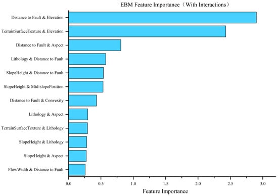
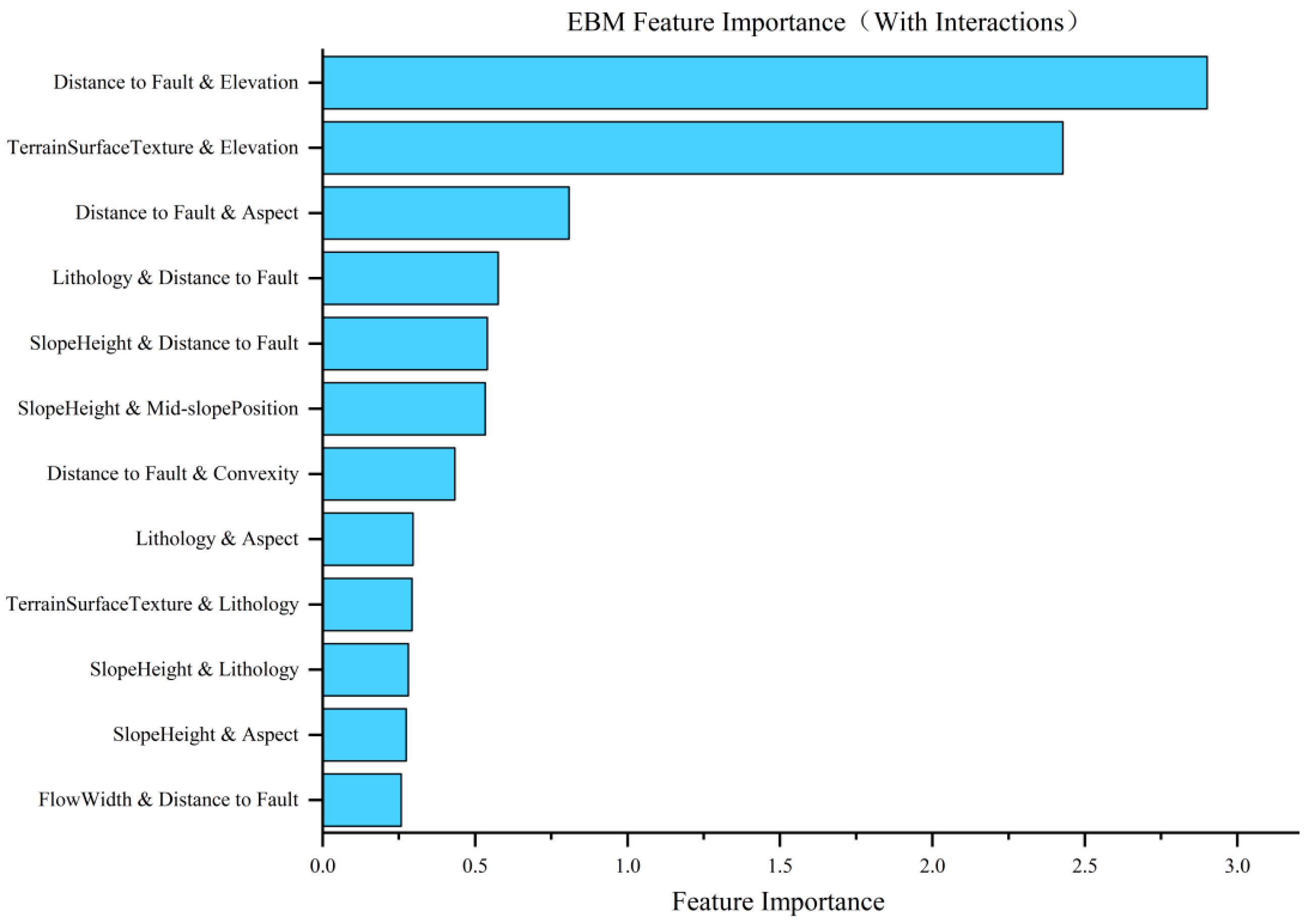
The three core factor sets mentioned above were trained using the same training set in combination with the EBM model, and the importance results of factor interactions were obtained, as shown in Figure 12.

Figure 12. EBM model factor interaction importance results.

As observed in Figure 12, the interaction between Distance to Fault and Elevation ranks first, while the interactions of Distance to Fault with Aspect and Slope Height rank third and fifth, respectively. Furthermore, it can be observed from the figure that there is no ranking for the interaction between Slope Length and other factors, indicating that the interactive effects of Slope Length with other factors are not ideal.

5.1.4. Accuracy Evaluation

(1)

ROC curves

The three core factor sets obtained in Section 5.1.1 were used for landslide susceptibility evaluation using the SVM model, with the resulting ROC curves and AUC values shown in Figure 13 and Table 7. The highest AUC value was achieved by PI-8 (0.931), differing by only 0.03 from the 13 factors (0.934), while the lowest was SHAP-8 (0.924), but both are higher than the AUC-RFE value of 0.918.

Figure 13. ROC curves.

Table 7. Area under the curve analysis.

Statistical Test Results	Area	Standard Deviation a	Asymptotic Sig. b	Asymptotic 95% Confidence Interval
				Lower Bound	Upper Bound
13 Factors	0.934	0.001	0.000	0.933	0.935
LIME-8	0.927	0.001	0.000	0.926	0.928
SHAP-8	0.924	0.001	0.000	0.923	0.925
PI-8	0.931	0.001	0.000	0.930	0.932
AUC-RFE-8	0.918	0.001	0.000	0.917	0.919

Note: a. under the non-parametric assumption; b. null hypothesis: actual area = 0.5.

(2)

Specific Category Accuracy Analysis

To enhance the readability of the landslide susceptibility evaluation results, the model prediction results were classified into five susceptibility zones—very low susceptibility, low susceptibility, moderate susceptibility, high susceptibility, and very high susceptibility—based on the intervals of 0–0.5, 0.5–0.70, 0.70–0.80, 0.80–0.90, and 0.90–1—with the results shown in Table 8. As can be observed from Table 8, among the three methods, SHAP-8 achieves the highest value of 48.80%, followed by PI-8 at 48.22%, and LIME-8 at the lowest of 47.85%. The smallest gap between the results of the 13-factor model is only 0.49%.

Table 8. Specific category accuracy analysis.

Category	Very Low (%)	Low (%)	Moderate (%)	High (%)	Very High (%)
13 Factors	0.85	9.87	18.15	30.73	49.29
LIME-8	0.90	9.89	19.44	30.57	47.85
SHAP-8	0.84	9.91	17.33	27.89	48.80
PI-8	0.85	9.89	18.95	30.69	48.22
AUC-RFE-8	0.89	9.68	18.00	30.13	48.23

(3)

Five Statistical Measures

The results of PI were analyzed using five statistical metrics, with the outcomes shown in Table 9. As shown in the table, the PI-8 group achieved the best performance (83.35%, 0.2627, 0.8956, 0.4063, and 0.4504). It outperformed both the LIME-8 and SHAP-8 groups across all metrics except recall, where its result was slightly inferior to that of the SHAP-8 group (0.8996).

Table 9. Five statistical measures.

Measures	OA	Precision	Recall	F-Measure	MCC
13 Factors	83.95%	0.2701	0.8944	0.4149	0.4578
LIME-8	83.10	0.2589	0.8896	0.4011	0.4458
SHAP-8	81.24%	0.2400	0.8996	0.3789	0.4266
PI-8	83.35%	0.2627	0.8956	0.4063	0.4504
AUC-RFE-8	80.37%	0.2310	0.8955	0.3672	0.4163

5.1.5. Result Validation

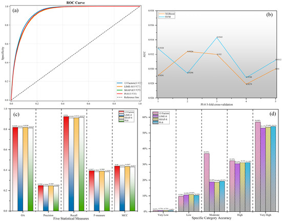
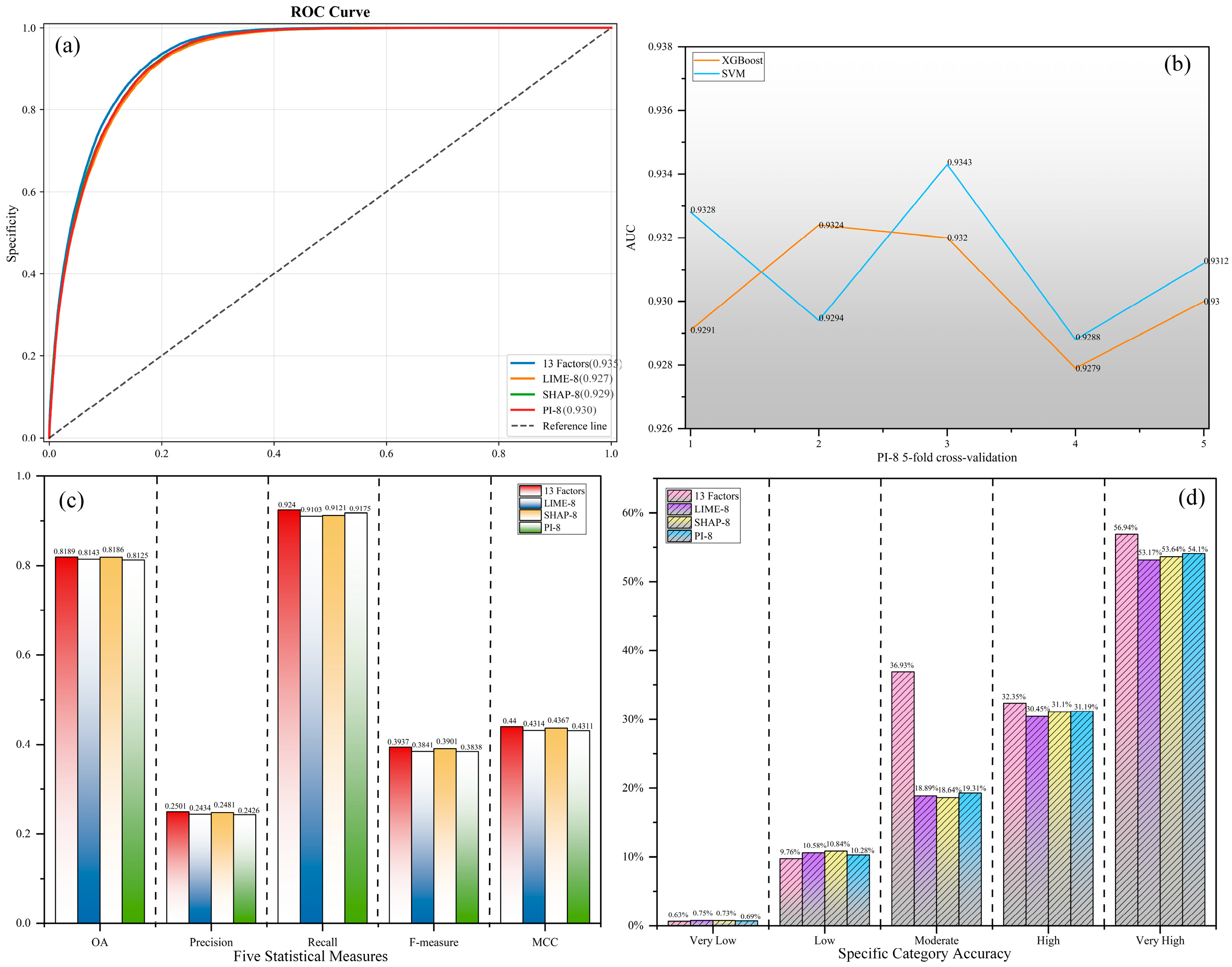
To ensure the objectivity of the results, the XGBoost model was additionally adopted for re-verification, and the five-fold cross-validation results of the PI-8 factor set are shown in Figure 14. It can be observed from Figure 14a,c,d that the AUC values, class-specific accuracies, and five statistical metrics derived from the XGBoost model are similar to those obtained with the SVM model in all aspects. The five-fold cross-validation results in Figure 14b are also consistent. Therefore, the PI-8 core factor set outperforms the other two sets.

Figure 14. XGBoost validation results ((a) ROC curve; (b) PI-8 5-fold cross-validation; (c) five statistical measures; (d) specific category accuracy).

Meanwhile, two traditional feature selection methods, namely, Information Gain (IG) and ReliefF, were selected for further comparison with the results presented above. The AUC values under different numbers of factors using Information Gain are IG-6: 0.903, IG-7: 0.907, and IG-8: 0.916, respectively. The corresponding results obtained by the ReliefF algorithm are ReliefF-6: 0.910, ReliefF-7: 0.919, and ReliefF-8: 0.919. It can be concluded that the core factor combination derived from the interpretable machine learning model still outperforms these two feature selection methods.

5.1.6. Core Factor Set Screening Results

Based on the comprehensive synthesis of all the aforementioned experiments, the AUC values of the SHAP-8 and LIME-8 groups (both containing the Slope Length factor) are inferior to that of the PI-8 group. Although the SHAP-8 group achieves a slightly higher accuracy in the extremely high susceptibility zone in the specific category accuracy analysis, it underperforms the PI-8 group across the five statistical metrics. Additionally, the interaction analysis of the EBM model in Figure 12 reveals that the interaction capability of the Slope Length factor is weaker than that of the other two distinct factors.

Therefore, considering all the results comprehensively, the number of core factors in the core factor set for the study area is determined to be eight, namely, Elevation, Slope, Terrain Surface Texture, Lithology, Distance to Fault, Mid-slope Position, Slope Height, and Aspect.

5.2. Core Factor Set Analysis

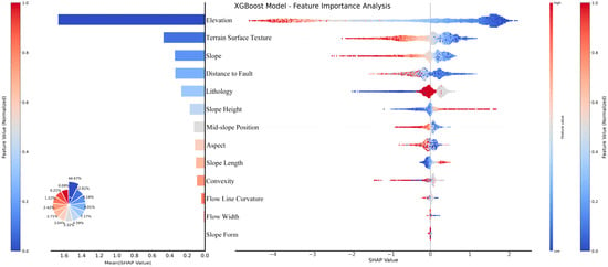
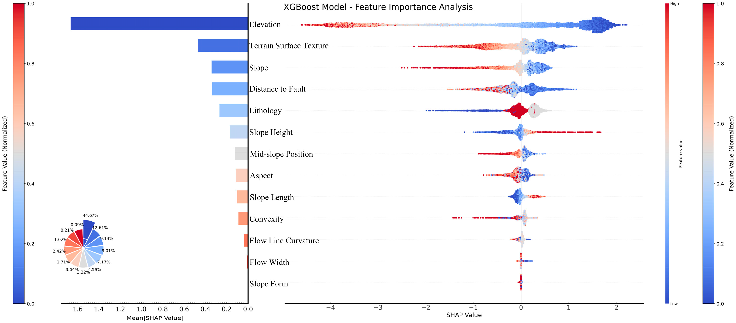
To analyze the statistical relationships between the core factor set and landslide development, machine learning models alone are insufficient to identify the influence thresholds, operational patterns of the factors within this core set, and the distribution of landslides under individual factors. Therefore, it is necessary to introduce the SHAP Beeswarm Plot to analyze the distribution characteristics of factor importance. The SHAP Beeswarm Plot can quantify the contribution of each factor to the model’s predictions. In the plot, a redder color indicates a larger feature value, while a bluer color represents a smaller feature value. The horizontal axis denotes the SHAP value: positive values signify a positive impact, and negative values indicate a negative impact, enabling an intuitive visualization of the factors’ influence on the prediction results [61]. The SHAP Beeswarm plot generated based on the XGBoost model is shown in Figure 15.

Figure 15. SHAP Beeswarm Plot.

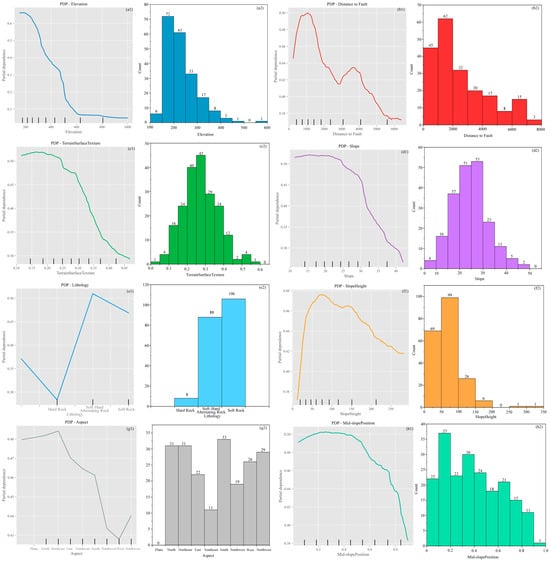
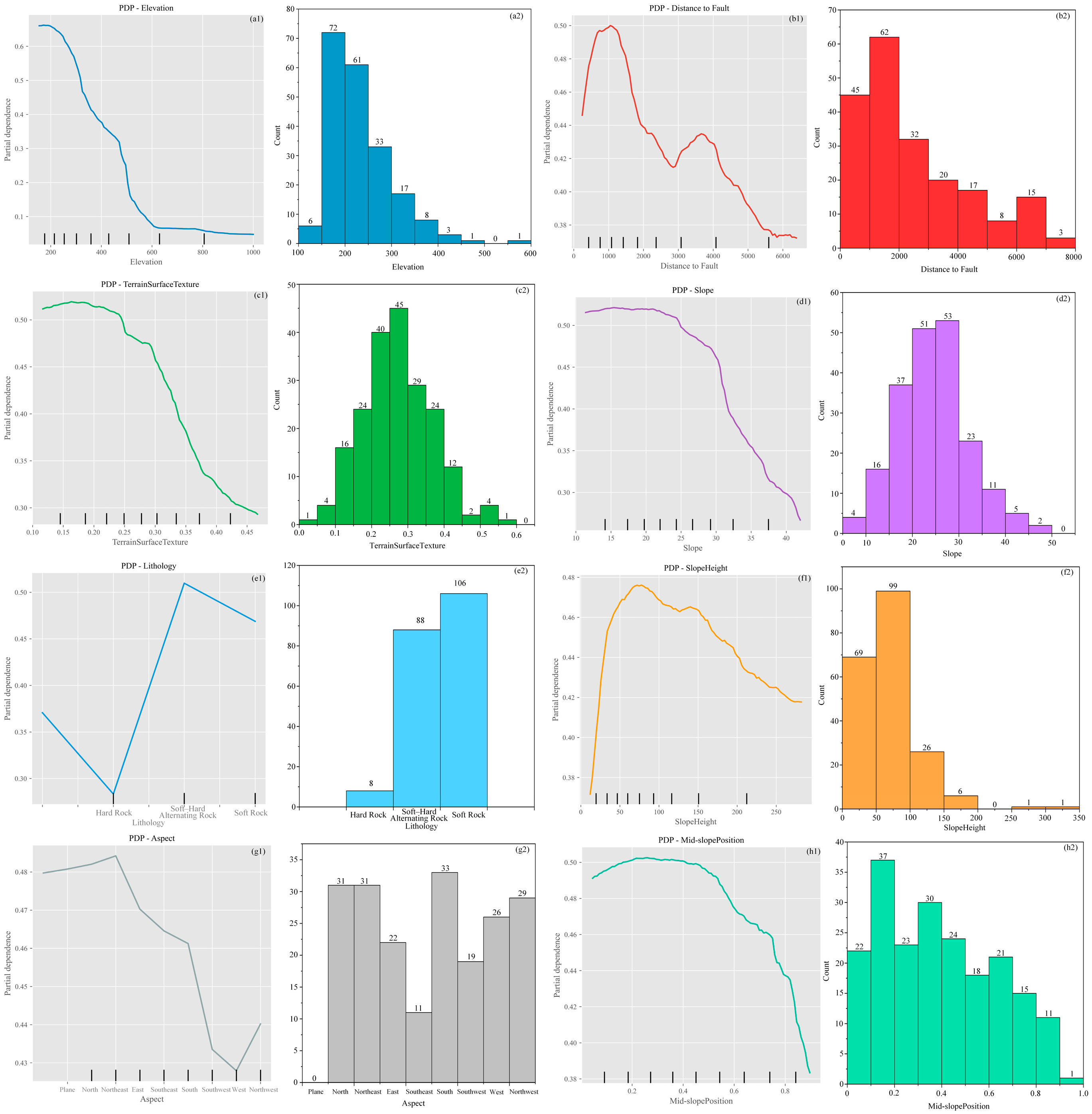
The Partial Dependence Plot (PDP) can intuitively demonstrate the relationship between single or two features and the model’s predicted outcomes, providing explanations for machine learning models and helping the user to understand how features influence the model’s predictions [62]. PDPs were generated based on the RF model, as shown in Figure 16(a1–h1). Meanwhile, to intuitively observe the distribution of landslides with respect to each factor, the central points of 202 landslides were extracted using ArcGIS 10.8. The data for the eight factors in the core factor set were then extracted and assigned to these landslide points, respectively, yielding the distribution characteristics of landslides across each factor. Finally, the landslide distribution maps were integrated with the corresponding factor-specific PDP graphs, and the results are shown in Figure 16(a2–h2). Furthermore, to explore the connections between statistical simulation results, actual landslide distribution, and geological principles, the relationships between the top-ranked factors and landslide development are shown in Table 10.

Figure 16. PDP and landslide distribution map ((a1,a2) Elevation; (b1,b2) Distance to Fault; (c1,c2) Terrain Surface Texture; (d1,d2) Slope; (e1,e2) Lithology; (f1,f2) Slope Height; (g1,g2) Aspect; (h1,h2) Mid-slope Position).

Table 10. Relationship between factors and landslides.

Factor	Statistical Relationship with Landslide Development	Geological Principle Linking to Landslide Development
Elevation	As the most influential factor, Elevation exhibits an overall negative correlation with landslide occurrence. It contributes the most to the prediction results within the range of 200–600 m, while exerting a certain inhibitory effect on landslides above 600 m, as shown in Figure 16(a1,a2).	Areas with lower elevation are typically close to rivers, resulting in high soil moisture content. In contrast, regions at higher elevation exhibit insignificant sediment accumulation [63], are generally sparsely populated with minimal human activity, and feature higher vegetation coverage and stronger soil and water conservation capacity [64,65].
Distance to Fault	As shown in Figure 16(b1,b2), Distance to Fault exerts the greatest influence on landslides within the range of 0–2500 m, with another small peak appearing around 3500 m. Overall, however, the farther the distance from the fault, the less likely landslides are to occur.	Fault structures are closely related to landslide development, and the influence of tectonic movements on landslide development decreases with increasing distance from the fault [66].
Terrain Surface Texture	As shown in Figure 16(c1,c2), Terrain Surface Texture exerts the greatest influence on landslides when its value is less than 0.40 within the study area.	It is a key indicator for measuring the complexity of the Earth’s surface: higher values typically correspond to landforms with significant relief such as mountain ridges or valleys, while lower values are associated with flat areas. Barman et al. found in their research that among the selected factors, Terrain Surface Texture ranked second in weight. Additionally, Kadavi et al. and Lee et al. also regarded it as a favorable factor [67].
Slope	As shown in Figure 16(d1,d2), for the Slope factor, the influence of gradient on landslide development is mainly concentrated within the range of 20–40°. The impact intensity in this range is higher than the landslide probability corresponding to gentler or steeper slopes.	Qiu et al. in Shaanxi Province and Liu et al. in Wenchuan discovered similar findings that landslides predominantly occurred on slopes with gradients between 30 and 40° [68,69]. Areas with gentle terrain and small slopes do not have the conditions for landslide hazards to occur, while rock wall areas with excessively steep slopes usually lack sufficient thickness of the weathered layer, making it difficult to form the material basis for landslides [70].
Lithology	As can be found, when the lithology is soft rock or soft–hard alternating rock, its influence on landslides is greater than that of hard rock. Moreover, soft–hard alternating rock is more prone to landslides than pure soft rock or hard rock, as shown in Figure 16(e1,e2).	Landslides are highly susceptible to lithology. Landslides are prone to occur when weak lithology or hard lithology is coupled with high and steep terrain, while lithology with a soft–hard alternating structure tends to form high-position and high-potential-energy initiation zones, providing the spatial conditions for the occurrence of landslide hazards [71,72].
Slope Height	Within the study area, landslides occur most frequently when slope heights are between 0 and 100 m, exhibiting a positive influence on prediction outcomes. Beyond 100 m, this influence gradually diminishes, as illustrated in Figure 16(f1,f2).	Slope height, as one of the primary factors influencing landslide development, affects stress distribution within slopes when it varies and, under certain conditions, provides potential energy for landslide initiation [73]. Zhang et al. found in their study in Sichuan Province that landslides mostly occurred within the slope height range of 0–84.55 m [74].
Aspect	As shown in Figure 16(g1,g2), the Southeast aspect contributes the least to model predictions, while the Northeast, South, and West aspects exhibit relatively higher contributions. Other aspects also influence predictions to varying degrees.	In landslide susceptibility mapping, slope aspect is a critical factor. Different aspects influence land cover, soil infiltration capacity, climate conditions, and weathering processes, leading to variations in vegetation coverage, weathering intensity, and evaporation rates, ultimately affecting landslide occurrence [75]. Additionally, the stability of geomaterials is partially governed by slope aspect, as seismic energy propagates more intensely perpendicular to fault strikes, resulting in uneven distribution of geohazards across different aspects [76].
Mid-slope Position	Slope position exhibits a segmented impact on landslide prediction. The lower and lower-middle sections, featuring stable stress conditions and dense materials, exert a steady influence on landslides with relatively low model sensitivity. In contrast, the influence on the model gradually increases in the middle and upper-middle sections, as illustrated in Figure 16(h1,h2).	Landslides predominantly develop in the upper-middle and upper sections of slopes. The most intense rock mass unloading deformation occurs in these areas, resulting in poorer stability that favors landslide initiation [77].

Through the analysis of Figure 15 and Figure 16 and Table 10, it is evident that the interpretations provided by the SHAP Beeswarm Plot and PDP are generally consistent in their overall results. These findings align well with the actual distribution of landslides under each factor within the study area. Moreover, the influence patterns of these factors on landslides are similar to those reported in previous studies, demonstrating that the core factor set derived through machine learning interpretability methods is scientifically robust and reliable.

Based on all the comprehensive results above, the top eight factors from the factor combinations obtained by each machine learning interpretability method were selected. Among them, six factors are consistent across all combinations, namely, Elevation, Slope, Terrain Surface Texture, Lithology, Distance to Fault, and Mid-slope Position. The differing factors include Slope Height, Slope Length, and Aspect. Through evaluations using ROC curves, specific category accuracy, five statistical measures, factor interaction analysis of the EBM model, SHAP Beeswarm Plot, PDPs, and landslide distribution patterns, the worst-performing factor (Slope Length) was eliminated. The core factor set for the study area was ultimately determined as Elevation, Slope, Terrain Surface Texture, Lithology, Distance to Fault, Mid-slope Position, Slope Height, and Aspect.

6. Conclusions and Prospects

6.1. Conclusions

Taking the Zigui–Badong section of the TGRA as the study case, this paper initially selected 25 landslide-related factors within the region based on previous research. After conducting PCC analysis and multicollinearity analysis, factors with a PCC value greater than 0.5 or a VIF greater than 10 were eliminated, resulting in 13 remaining factors. The SHAP, LIME, and AUC-RFE methods were employed to perform a preliminary ranking of factor importance. Synthesizing the ranking results of the three methods, the top six, seven, and eight factors from each method were selected, respectively, as candidate core factor sets for experimentation. It was found that the AUC values, specific category accuracy, and five statistical measures of the core factor sets screened by each method all increased with the increase in the number of factors. When the number of core factors in each method reached eight, the performance results were comparable to those of the original 13 factor set.

Since the eight factors screened by SHAP and LIME failed to reach a consensus, two additional methods, namely, PI and EBM, were incorporated for further analysis and discussion. After obtaining the factor importance ranking derived from the PI method, an analysis was conducted on the ranking consistency of the three methods, which revealed a high level of consistency among them. It was found that there were six common factors ranked within the top eight by all three methods, along with three pending factors. Further analysis and verification were performed using the interaction function of the EBM model, and the results indicated that the importance of Slope Length was weaker than that of the other two pending factors. After verifying and analyzing all the results, the core factor set for the study area was finally determined to consist of the following eight factors: Elevation, Slope, Terrain Surface Texture, Lithology, Distance to Fault, Mid-slope Position, Slope Height, and Aspect.

In this study, the Pearson correlation coefficient (PCC) and Variance Inflation Factor (VIF) were first employed to eliminate redundant factors. Subsequently, multiple machine learning interpretability methods were adopted to screen, verify, and analyze the core factor set within the study area, and the core factor set suitable for the study area was finally determined. This demonstrates that interpretable machine learning models are applicable to factor selection, and the ranking of factors derived from these interpretability methods exhibits more stable consistency. This study provides a reproducible approach for landslide factor screening in geologically complex areas such as the Three Gorges Reservoir Area. It also supplements the theoretical research on landslide formation in the TGRA, and offers a basis for the selection of landslide susceptibility assessment factors in the reservoir area in subsequent studies. Meanwhile, it reduces the computational cost and data acquisition difficulty of regional landslide prediction models. The clearly defined core factor system enables efficient assessment of landslide risks, provides a scientific basis for engineering prevention and control in the TGRA, and contributes to enhancing the precision and cost-effectiveness of landslide disaster prevention and control in this region.

6.2. Prospects

This study has certain limitations in the selection of prediction and validation methods, as only tree-based models and the SVM model were adopted, without considering the applicability of other models such as KNN and ANN. In future research, more diverse machine learning models will be included, and deep learning models such as CNN and neural networks will be introduced for a more comprehensive comparison. Meanwhile, various models will be used to verify the method proposed in this study.

In terms of data, the 202 landslide samples may be insufficient for deep learning model training. In the follow-up research, more landslide samples will be collected, especially newly discovered and recently occurring landslide events, to expand the sample size. In addition, detailed historical rainfall records of the study area (e.g., average annual rainfall, extreme rainfall events) will be collected, and rainfall factors will be incorporated into the factor set analysis to improve the comprehensiveness of factor selection. The interaction mechanism among core factors and their impacts on landslide occurrence will be analyzed, so as to enrich the theoretical research on landslide formation in the Three Gorges Reservoir Area.

In summary, future research will focus on method optimization, data quality improvement, and in-depth result interpretation, aiming to enhance the scientificity and practical value of the study, and provide more reliable support for landslide disaster prevention and mitigation in the Three Gorges Reservoir Area and similar regions.

References

- Zhou, D.; Zhao, Z.; Xi, W.; Zhao, X.; Chao, J. New method for landslide susceptibility evaluation in alpine valley regions that considers the suitability of InSAR monitoring and introduces deformation rate grading. Geo-Spat. Inf. Sci. 2025, 28, 565–588. [Google Scholar] [CrossRef] [Scilit]
- Sahrane, R.; Bounab, A.; El Kharim, Y.; Obda, O.; El Miloudi, Y.; Mihraje, A.I.; Ahniche, M.; El Afi, M. Landslide–Anthropogenic Interactions in Urban Areas: A Multidisciplinary Case Study from Taounate, Morocco. Geotech. Geol. Eng. 2025, 43, 238. [Google Scholar] [CrossRef] [Scilit]
- Fan, X.; Wang, X.; Fang, C.; Jansen, J.D.; Dai, L.; Tanyas, H.; Zang, N.; Tang, R.; Xu, Q.; Huang, R. Deep learning can predict global earthquake-triggered landslides. Natl. Sci. Rev. 2025, 12, nwaf179. [Google Scholar] [CrossRef] [Scilit]
- Hussain, S.; Sun, H.X.; Ali, M.; Sajjad, M.M.; Ali, M.; Afzal, Z.; Ali, S. Optimized landslide susceptibility mapping and modelling using PS-InSAR technique: A case study of Chitral valley, Northern Pakistan. Geocarto Int. 2021, 37, 5227–5248. [Google Scholar] [CrossRef] [Scilit]
- Xia, L.; Shen, J.; Zhang, T.; Dang, G.; Wang, T. GIS-based landslide susceptibility modeling using data mining techniques. Front. Earth Sci. 2023, 11, 1187384. [Google Scholar] [CrossRef] [Scilit]
- Meena, S.R.; Puliero, S.; Bhuyan, K.; Floris, M.; Catani, F. Assessing the importance of conditioning factor selection in landslide susceptibility for the province of Belluno (region of Veneto, northeastern Italy). Nat. Hazards Earth Syst. Sci. 2022, 22, 1395–1417. [Google Scholar] [CrossRef] [Scilit]
- Kincal, C.; Kayhan, H. A Combined Method for Preparation of Landslide Susceptibility Map in Izmir (Türkiye). Appl. Sci. 2022, 12, 9029. [Google Scholar] [CrossRef] [Scilit]
- Panchal, S.; Shrivastava, A.K. Landslide hazard assessment using analytic hierarchy process (AHP): A case study of National Highway 5 in India. Ain Shams Eng. J. 2022, 13, 101671. [Google Scholar] [CrossRef] [Scilit]
- Liu, X.K.; Shao, S.; Shao, S.J. Landslide susceptibility prediction and mapping in Loess Plateau based on different machine learning algorithms by hybrid factors screening: Case study of Xunyi County, Shaanxi Province, China. Adv. Space Res. 2024, 74, 192–210. [Google Scholar] [CrossRef] [Scilit]
- Zhou, J.; Tan, S.; Li, J.; Xu, J.; Wang, C.; Ye, H. Landslide Susceptibility Assessment Using the Analytic Hierarchy Process (AHP): A Case Study of a Construction Site for Photovoltaic Power Generation in Yunxian County, Southwest China. Sustainability 2023, 15, 5281. [Google Scholar] [CrossRef] [Scilit]
- Rebouh, N.; Belkendil, A.; Tout, F.; Dinar, H.; Benzid, Y.; Zeghmar, A.; Alliouche, A.; Farah, M.I.; Najar, I.A.; Khan, N.A. Landslide susceptibility assessment using hybrid geospatial, frequency ratio, and AHP models in Souk Ahras province, Northeastern of Algeria. Sci. Rep. 2026, 16, 2288. [Google Scholar] [CrossRef] [Scilit]
- Peng, L.; Sun, Y.; Zhan, Z.; Shi, W.; Zhang, M. FR-weighted GeoDetector for landslide susceptibility and driving factors analysis. Geomat. Nat. Hazards Risk 2023, 14, 2205001. [Google Scholar] [CrossRef] [Scilit]
- Yu, L.; Wang, Y. Pradhan B Enhancing landslide susceptibility mapping incorporating landslide typology via stacking ensemble machine learning in Three Gorges Reservoir, China. Geosci. Front. 2024, 15, 101802. [Google Scholar] [CrossRef] [Scilit]
- Wang, Y.; Zhang, Z.; Yu, X.; Liu, C. Landslide susceptibility assessment via the information value-coupled machine learning models. PLoS ONE 2025, 20, e0333055. [Google Scholar] [CrossRef] [Scilit] [PubMed]
- Can, R.; Kocaman, S.; Gokceoglu, C. A Comprehensive Assessment of XGBoost Algorithm for Landslide Susceptibility Mapping in the Upper Basin of Ataturk Dam, Turkey. Appl. Sci. 2021, 11, 4993. [Google Scholar] [CrossRef] [Scilit]
- Hussain, M.A.; Chen, Z.; Zheng, Y.; Zhou, Y.; Daud, H. Deep Learning and Machine Learning Models for Landslide Susceptibility Mapping with Remote Sensing Data. Remote Sens. 2023, 15, 4703. [Google Scholar] [CrossRef] [Scilit]
- Sun, D.; Gu, Q.; Wen, H.; Shi, S.; Mi, C.; Zhang, F. A Hybrid Landslide Warning Model Coupling Susceptibility Zoning and Precipitation. Forests 2022, 13, 827. [Google Scholar] [CrossRef] [Scilit]
- Ribeiro, M.T.; Singh, S.; Guestrin, C. “Why should i trust you?”: Explaining the predictions of any classifier. In Proceedings of the 22nd ACM SIGKDD International Conference on Knowledge Discovery and Data Mining-KDD’16, San Francisco, CA, USA, 13–17 August 2016; ACM Press: New York, NY, USA, 2016. [Google Scholar] [CrossRef] [Scilit]
- Yan, X.; Zhang, D.; Han, Y.; Li, T.; Zhong, P.; Ning, Z.; Tan, S. Developing a Hybrid Model to Enhance the Robustness of Interpretability for Landslide Susceptibility Assessment. ISPRS Int. J. Geo-Inf. 2025, 14, 277. [Google Scholar] [CrossRef] [Scilit]
- Alqadhi, S.; Mallick, J.; Alkahtani, M.; Ahmad, I.; Alqahtani, D.; Hang, H.T. Developing a hybrid deep learning model with explainable artificial intelligence (XAI) for enhanced landslide susceptibility modeling and management. Nat. Hazards 2023, 120, 3719–3747. [Google Scholar] [CrossRef] [Scilit]
- Bostan, T. Generating a Landslide Susceptibility Map Using Integrated Meta-Heuristic Optimization and Machine Learning Models. Sustainability 2024, 16, 9396. [Google Scholar] [CrossRef] [Scilit]
- Teke, A.; Kavzoglu, T. Exploring the decision-making process of ensemble learning algorithms in landslide susceptibility mapping: Insights from local and global explainable AI analyses. Adv. Space Res. 2024, 74, 3765–3785. [Google Scholar] [CrossRef] [Scilit]
- Lin, N.; Ding, K.; Tan, L.; Li, B.; Yang, K.; Wang, C.; Wang, B.; Li, N.; Yang, R. Dynamic landslide susceptibility mapping on time-series InSAR and explainable machine learning: A case study at Wushan in the Three Gorges Reservoir area, China. Adv. Space Res. 2025, 75, 8439–8465. [Google Scholar] [CrossRef] [Scilit]
- Wang, P.; Deng, H. The impact of different sampling strategies on landslide susceptibility assessment: An explainable hybrid BO-XGBoost model. Earth Sci. Inform. 2025, 18, 440. [Google Scholar] [CrossRef] [Scilit]
- Le, X.H.; Choi, C.; Eu, S.; Yeon, M.; Lee, G. Quantitative evaluation of uncertainty and interpretability in machine learning-based landslide susceptibility mapping through feature selection and explainable AI. Front. Environ. Sci. 2024, 12, 1424988. [Google Scholar] [CrossRef] [Scilit]
- Lv, J.; Zhang, R.; Shama, A.; Hong, R.K.; He, X.; Wu, R.Z.; Bao, X.; Liu, G.X. Exploring the spatial patterns of landslide susceptibility assessment using interpretable Shapley method: Mechanisms of landslide formation in the Sichuan-Tibet region. J. Environ. Manag. 2024, 366, 121921. [Google Scholar] [CrossRef] [Scilit]
- Song, Y.; Niu, R.; Xu, S.; Ye, R.; Peng, L.; Guo, T.; Li, S.; Chen, T. Landslide Susceptibility Mapping Based on Weighted Gradient Boosting Decision Tree in Wanzhou Section of the Three Gorges Reservoir Area (China). ISPRS Int. J. Geo-Inf. 2019, 8, 4. [Google Scholar] [CrossRef] [Scilit]
- Li, Y.; Xie, X.; Jin, B.; Chen, L.; Liang, X.; Yin, K. Comprehensive risk management of reservoir landslide-tsunami hazard chains: A case study of the Liangshuijing landslide in the Three Gorges Reservoir area. Landslides 2025, 22, 671–691. [Google Scholar] [CrossRef] [Scilit]
- Tang, H.; Wasowski, J.; Juang, C.H. Geohazards in the three Gorges Reservoir Area, China-Lessons learned from decades of research. Eng. Geol. 2019, 261, 105267. [Google Scholar] [CrossRef] [Scilit]
- Peng, B.; Wu, X. Optimizing rainfall-triggered landslide thresholds for daily landslide hazard warning in the Three Gorges Reservoir area. Nat. Hazards Earth Syst. Sci. 2024, 24, 3991–4013. [Google Scholar] [CrossRef] [Scilit]
- Fan, Z.; Wang, S.; Wang, L.; Guo, F.; Nan, F.; Hu, Y. Emergency treatment effect evaluation of rear-slope cutting and front-slope pressing on a hydrodynamic pressure landslide: A case study of the Shuping landslide in the Three Gorges Reservoir Area. Bull. Eng. Geol. Environ. 2024, 83, 38. [Google Scholar] [CrossRef] [Scilit]
- Luo, S.; Huang, D.; Peng, J.; Xie, Z.; Yang, Z.; Tomás, R. Insights into Reservoir-Triggered Landslides Development and Its Influence Factors in the Three Gorges Reservoir Area, China. J. Earth Sci. 2024, 35, 1979–1997. [Google Scholar] [CrossRef] [Scilit]
- Li, W.; Fang, Z.; Wang, Y. Stacking ensemble of deep learning methods for landslide susceptibility mapping in the Three Gorges Reservoir area, China. Stoch. Environ. Res. Risk Assess. 2021, 36, 2207–2228. [Google Scholar] [CrossRef] [Scilit]
- He, L.; Wu, X.; He, Z.; Xue, D.; Luo, F.; Bai, W.; Kang, G.; Chen, X.; Zhang, Y. Susceptibility Assessment of Landslides in the Loess Plateau Based on Machine Learning Models: A Case Study of Xining City. Sustainability 2023, 15, 14761. [Google Scholar] [CrossRef] [Scilit]
- Shahabi, H.; Ahmadi, R.; Alizadeh, M.; Hashim, M.; Al-Ansari, N.; Shirzadi, A.; Wolf, I.D.; Ariffin, E.H. Landslide Susceptibility Mapping in a Mountainous Area Using Machine Learning Algorithms. Remote Sens. 2023, 15, 3112. [Google Scholar] [CrossRef] [Scilit]
- Lin, N.; Zhang, D.; Feng, S.; Ding, K.; Tan, L.; Wang, B.; Chen, T.; Li, W.; Dai, X.; Pan, J.; et al. Rapid Landslide Extraction from High-Resolution Remote Sensing Images Using SHAP-OPT-XGBoost. Remote Sens. 2023, 15, 3901. [Google Scholar] [CrossRef] [Scilit]
- Dai, X.; Chen, J.; Zhang, T.; Xue, C. Integrated Landslide Risk Assessment via a Landslide Susceptibility Model Based on Intelligent Optimization Algorithms. Remote Sens. 2025, 17, 545. [Google Scholar] [CrossRef] [Scilit]
- Chang, Z.L.; Huang, F.M.; Huang, J.S.; Jiang, S.H.; Liu, Y.T.; Meena, S.R.; Catani, F. An updating of landslide susceptibility prediction from the perspective of space and time. Geosci. Front. 2023, 14, 101619. [Google Scholar] [CrossRef] [Scilit]
- Visani, G.; Bagli, E.; Chesani, F.; Poluzzi, A.; Capuzzo, D. Statistical stability indices for LIME: Obtaining reliable explanations for machine learning models. J. Oper. Res. Soc. 2022, 73, 91–101. [Google Scholar] [CrossRef] [Scilit]
- Sun, D.L.; Ding, Y.K.; Wen, H.J.; Zhang, F.T.; Zhang, J.Y.; Gu, Q.Y.; Zhang, J.L. SHAP-PDP hybrid interpretation of decision-making mechanism of machine learning-based landslide susceptibility mapping: A case study at Wushan District, China. Egypt. J. Remote Sens. Space Sci. 2024, 27, 508–523. [Google Scholar] [CrossRef] [Scilit]
- Lundberg, S.; Lee, S.I. A Unified Approach to Interpreting Model Predictions. Adv. Neural Inf. Process. Syst. 2017, 30, 4768–4777. [Google Scholar] [CrossRef] [Scilit]
- Halder, K.; Srivastava, A.K.; Ghosh, A.; Das, S.; Banerjee, S.; Pal, S.C.; Chatterjee, U.; Bisai, D.; Ewert, F.; Gaiser, T. Publisher Correction: Improving landslide susceptibility prediction through ensemble recursive feature elimination and meta-learning framework. Sci. Rep. 2025, 15, 5170. [Google Scholar] [CrossRef] [Scilit] [PubMed]
- Hu, L.; Yan, C. Evaluation of Landslide Susceptibility of Mangshan Mountain in Zhengzhou Based on GWO-1D CNN Model. Sustainability 2024, 16, 5086. [Google Scholar] [CrossRef] [Scilit]
- Li, X.; Li, W.; Wu, Z.; Xu, Q.; Zheng, D.; Dong, X.; Lu, H.; Shan, Y.; Zhou, S.; Yu, W.; et al. Identification and Deformation Characteristics of Active Landslides at Large Hydropower Stations at the Early Impoundment Stage: A Case Study of the Lianghekou Reservoir Area in Sichuan Province, Southwest China. Remote Sens. 2024, 16, 3175. [Google Scholar] [CrossRef] [Scilit]
- Cheng, J.; Sun, J.; Yao, K.; Xu, M.; Cao, Y. A variable selection method based on mutual information and variance inflation factor. Spectrochim. Acta Part. A Mol. Biomol. Spectrosc. 2021, 268, 120652. [Google Scholar] [CrossRef] [Scilit]
- Wang, Z.; Ma, C.; Qiu, Y.; Xiong, H.; Li, M. Refined Zoning of Landslide Susceptibility: A Case Study in Enshi County, Hubei, China. Int. J. Environ. Res. Public Health 2022, 19, 9412. [Google Scholar] [CrossRef] [Scilit]
- Yu, X.; Chen, H. Research on the influence of different sampling resolution and spatial resolution in sampling strategy on landslide susceptibility mapping results. Sci. Rep. 2024, 14, 1549. [Google Scholar] [CrossRef] [Scilit] [PubMed]
- Fang, Z.; Wang, Y.; Peng, L.; Hong, H. Integration of convolutional neural network and conventional machine learning classifiers for landslide susceptibility mapping. Comput. Geosci. 2020, 139, 104470. [Google Scholar] [CrossRef] [Scilit]
- Ferreira, Z.; Almeida, B.; Costa, A.C.; Fernandes, M.C.; Cabral, P. Insights into landslide susceptibility: A comparative evaluation of multi-criteria analysis and machine learning techniques. Geomat. Nat. Hazards Risk 2025, 16, 2471019. [Google Scholar] [CrossRef] [Scilit]
- Yu, X.; Xiong, T.; Jiang, W.; Zhou, J. Comparative Assessment of the Efficacy of the Five Kinds of Models in Landslide Susceptibility Map for Factor Screening: A Case Study at Zigui-Badong in the Three Gorges Reservoir Area, China. Sustainability 2023, 15, 800. [Google Scholar] [CrossRef] [Scilit]
- Tanyaş, H.; van Westen, C.J.; Allstadt, K.E.; Jibson, R.W. Factors controlling landslide frequency–area distributions. Earth Surf. Process. Landf. 2019, 44, 900–917. [Google Scholar] [CrossRef] [Scilit]
- Jiang, W.; Li, L.; Niu, R. Impact of Non-Landslide Sample Sampling Strategies and Model Selection on Landslide Susceptibility Mapping. Appl. Sci. 2025, 15, 2132. [Google Scholar] [CrossRef] [Scilit]
- Abdelkader, M.M.; Csámer, Á. Comparative assessment of machine learning models for landslide susceptibility mapping: A focus on validation and accuracy. Nat. Hazards 2025, 121, 10299–10321. [Google Scholar] [CrossRef] [Scilit]
- Kumar, C.; Walton, G.; Santi, P.; Luza, C. Random Cross-Validation Produces Biased Assessment of Machine Learning Performance in Regional Landslide Susceptibility Prediction. Remote Sens. 2025, 17, 213. [Google Scholar] [CrossRef] [Scilit]
- Kavzoglu, T.; Kutlug Sahin, E.; Colkesen, I. Selecting optimal conditioning factors in shallow translational landslide susceptibility mapping using genetic algorithm. Eng. Geol. 2015, 192, 101–112. [Google Scholar] [CrossRef] [Scilit]
- Ma, S.; Qiu, H.; Hu, S.; Pei, Y.; Yang, W.; Yang, D.; Cao, M. Quantitative assessment of landslide susceptibility on the Loess Plateau in China. Phys. Geogr. 2020, 41, 489–516. [Google Scholar] [CrossRef] [Scilit]
- Zhang, Y.; Zeng, Y.; Xu, P.; Liu, J.; Li, Z.; Sun, Y.; Feng, Z. Effects of combination of influencing factors on earthquake-induced landslide susceptibility assessments. Environ. Earth Sci. 2025, 84, 189. [Google Scholar] [CrossRef] [Scilit]
- Mulabbi, A.; Danoedoro, P.; Samodra, G. Integrating interpretable artificial neural networks, geomorphic plausibility and transfer learning for landslide susceptibility mapping: A case study of Pacitan, East Java. Discov. Sustain. 2025, 6, 1159. [Google Scholar] [CrossRef] [Scilit]
- Umar, I.H.; Lin, H.; Hassan, J.I. Transforming Landslide Prediction: A Novel Approach Combining Numerical Methods and Advanced Correlation Analysis in Slope Stability Investigation. Appl. Sci. 2024, 14, 3685. [Google Scholar] [CrossRef] [Scilit]
- Arslan, A.K.; Yagin, F.H.; Algarni, A.; AL-Hashem, F.; Ardigò, L.P. Combining the Strengths of the Explainable Boosting Machine and Metabolomics Approaches for Biomarker Discovery in Acute Myocardial Infarction. Diagnostics 2024, 14, 1353. [Google Scholar] [CrossRef] [Scilit] [PubMed]
- Khan, D.; Akram, W.; Ullah, S. Enhancing landslide susceptibility predictions with XGBoost and SHAP: A data-driven explainable AI method. Geocarto Int. 2025, 40, 1. [Google Scholar] [CrossRef] [Scilit]
- Yang, Y.; Ma, X.; Ding, W.; Wen, H.; Sun, D. A Novel Dataset Replenishment Strategy Integrating Time-Series InSAR for Refined Landslide Susceptibility Mapping in Karst Regions. Water 2024, 16, 2414. [Google Scholar] [CrossRef] [Scilit]
- Wei, Z.L.; Wang, D.F.; Xu, H.D.; Sun, H.Y. Clarifying the effectiveness of drainage tunnels in landslide controls based on high-frequency in-site monitoring. Bull. Eng. Geol. Environ. 2020, 79, 3289–3305. [Google Scholar] [CrossRef] [Scilit]
- Wang, H.; Xu, J.; Tan, S.; Zhou, J. Landslide Susceptibility Evaluation Based on a Coupled Informative–Logistic Regression Model—Shuangbai County as an Example. Sustainability 2023, 15, 12449. [Google Scholar] [CrossRef] [Scilit]
- Tong, D.F.; Su, A.J.; Tan, F.; Tang, J.D.; Yi, X.W. Genetic mechanism of water-rich landslide considering antecedent rainfalls; A case study of Pingyikou landslide in Three Gorges Reservoir area. J. Earth Sci. 2023, 34, 1878–1891. [Google Scholar] [CrossRef] [Scilit]
- Ali, S.; Biermanns, P.; Haider, R.; Reicherter, K. Landslide susceptibility mapping by using a geographic information system (GIS) along the China–Pakistan Economic Corridor (Karakoram Highway), Pakistan. Nat. Hazards Earth Syst. Sci. 2019, 19, 999–1022. [Google Scholar] [CrossRef] [Scilit]
- Barman, J.; Biswas, B.; Rao, K.S. A hybrid integration of analytical hierarchy process (AHP) and the multiobjective optimization on the basis of ratio analysis (MOORA) for landslide susceptibility zonation of Aizawl, India. Nat. Hazards 2024, 120, 8571–8596. [Google Scholar] [CrossRef] [Scilit]
- Qiu, H.J.; Cui, Y.F.; Hu, S.; Yang, D.D.; Pei, Y.Q.; Ma, S.Y.; Liu, Z.J. Size distribution and size of loess slidesin response to slope height and slope gradient based on field survey data. Geomat. Nat. Hazards Risk 2019, 10, 1443–1458. [Google Scholar] [CrossRef] [Scilit]
- Liu, R.; Wang, T. The relationship between three-dimensional coseismic displacement and distribution of coseismic landslides. Sci. China Earth Sci. 2023, 66, 1583–1602. [Google Scholar] [CrossRef] [Scilit]
- Fusco, F.; Mirus, B.B.; Baum, R.L.; Calcaterra, D.; De Vita, P. Incorporating the Effects of Complex Soil Layering and Thickness Local Variability into Distributed Landslide Susceptibility Assessments. Water 2021, 13, 713. [Google Scholar] [CrossRef] [Scilit]
- Chen, G.; Cai, P.; Zhan, J.; Yang, Y.; Yao, Z.; Yu, Z. Deformation Patterns and Failure Mechanisms of Soft-Hard-Interbedded Anti-Inclined Layered Rock Slope in Wolong Open-Pit Coal Mine. Appl. Sci. 2024, 14, 3082. [Google Scholar] [CrossRef] [Scilit]
- Yu, X.; Zhang, K.; Song, Y.; Jiang, W.; Zhou, J. Study on landslide susceptibility mapping based on rock–soil characteristic factors. Sci. Rep. 2021, 11, 15476. [Google Scholar] [CrossRef] [Scilit]
- Qiu, H.; Regmi, A.D.; Cui, P.; Cao, M.; Lee, J.; Zhu, X. Size distribution of loess slides in relation to local slope height within different slope morphologies. Catena 2016, 145, 155–163. [Google Scholar] [CrossRef] [Scilit]
- Zhang, J.; Qian, J.; Lu, Y.; Li, X.; Song, Z. Study on Landslide Susceptibility Based on Multi-Model Coupling: A Case Study of Sichuan Province, China. Sustainability 2024, 16, 6803. [Google Scholar] [CrossRef] [Scilit]
- Chowdhury, M.S.; Rahman, M.N.; Sheikh, M.S.; Sayeid, M.A.; Mahmud, K.H.; Hafsa, B. GIS-based landslide susceptibility mapping using logistic regression, random forest and decision and regression tree models in Chattogram District, Bangladesh. Heliyon 2024, 10, e23424. [Google Scholar] [CrossRef] [Scilit] [PubMed]
- Martino, S.; Fiorucci, M.; Marmoni, G.M.; Casaburi, L.; Antonielli, B.; Mazzanti, P. Increase in landslide activity after a low-magnitude earthquake as inferred from DInSAR interferometry. Sci. Rep. 2022, 12, 2686. [Google Scholar] [CrossRef] [Scilit] [PubMed]
- Ambrosi, C.; Strozzi, T.; Scapozza, C.; Wegmüller, U. Landslide hazard assessment in the Himalayas (Nepal and Bhutan) based on Earth-Observation data. Eng. Geol. 2018, 237, 217–228. [Google Scholar] [CrossRef] [Scilit]
Disclaimer/Publisher’s Note: The statements, opinions and data contained in all publications are solely those of the individual author(s) and contributor(s) and not of MDPI and/or the editor(s). MDPI and/or the editor(s) disclaim responsibility for any injury to people or property resulting from any ideas, methods, instructions or products referred to in the content. |
© 2026 by the authors. Licensee MDPI, Basel, Switzerland. This article is an open access article distributed under the terms and conditions of the Creative Commons Attribution (CC BY) license.