


Abstract
This study aimed to enhance the accuracy and interpretability of erosion gully classification within black soil regions by focusing on Changxing Township, Xinxing District, Qitaihe City, Heilongjiang Province as the research site. Utilizing RTK (Real-Time Kinematic) surveying technology, three-dimensional topographic data were collected for 139 actively developing erosion gullies. Key morphological parameters—including gully length, depth, gradient, average top width, average bottom width, and slope gradients on both sides—were extracted to construct interactive features. The variable set was refined through correlation analysis and variance inflation factor (VIF) diagnostics to mitigate multicollinearity. A random forest model was employed as the primary classification approach and benchmarked against logistic regression, support vector machines (SVM), decision trees, and backpropagation neural networks. To address class imbalance, a combination of class weighting, Synthetic Minority Over-sampling Technique (SMOTE), and undersampling methods was implemented. Model tuning and interpretability assessments were performed using cross-validation, grid search optimization, and SHapley Additive exPlanations (SHAP) analysis. The findings demonstrate that the random forest model achieved superior overall performance, with test set accuracy, macro-averaged F1 score, and balanced accuracy values of 0.9143, 0.8087, and 0.8427, respectively. Among imbalance handling techniques, class weighting yielded better results compared to oversampling and undersampling. Feature importance and SHAP analyses identified gully length, average crest width, and their interaction with gully depth as the principal determinants influencing gully grade classification. These results elucidate the synergistic developmental dynamics of gully longitudinal extension, vertical deepening, and lateral widening. The proposed methodology offers valuable technical support for the rapid surveying, classification, and management decision-making processes related to black soil erosion gullies.
1. Introduction
Erosion gullies represent a significant geomorphological feature indicative of the progression of slope erosion, transitioning from diffuse surface and minor channel erosion to concentrated linear erosion. They serve as a critical process unit that integrates slope runoff generation, soil denudation, sediment transport, and landscape modification [1,2,3]. In comparison to sheet erosion or shallow gully erosion, erosion gullies are distinguished by their high erosion intensity, rapid spatial expansion, pronounced terrain degradation, and challenges in management. These features not only contribute to the fragmentation of agricultural land and the depletion of soil fertility but also increase sediment connectivity within watersheds, thereby influencing downstream river sedimentation patterns, reservoir longevity, and regional ecological stability [1,4,5,6]. Because of these combined on-site and off-site effects, gully erosion is widely regarded as one of the most destructive forms of water erosion and a major obstacle to sustainable land use in agricultural watersheds [2,5,6].
The policy and environmental significance of this problem is especially evident in the black soil region of Northeast China, which is one of the country’s most important grain-producing areas. According to recent official reports and special surveys, the black soil region contains 667,000 erosion gullies, with a total gully length of 232,400 km and an affected area of 4029.57 km2; nearly 90% of these gullies are still actively developing. Erosion gullies in this region have directly occupied or destroyed approximately 4.1772 million mu of cultivated land, thereby threatening farmland continuity, mechanized farming operations, and regional food security. Since 2017, central government investment in gully control has reached CNY 13.42 billion. During the 14th Five-Year Plan period, about 33,000 gullies were treated, protecting and restoring 7.92 million mu of farmland and increasing annual grain production capacity by about 190 million jin [7]. These figures indicate that erosion gullies are not merely local geomorphic features, but a major practical constraint on cultivated-land protection, sediment control, ecological restoration, and rural development policy in Northeast China. In recent years, under the compounded influences of global environmental change and intensified anthropogenic activities, erosion gullies have demonstrated significant spatial heterogeneity and complex developmental dynamics across various climatic zones and land-use types. The processes governing their formation, expansion, and stabilization are controlled by an interplay of multiple factors, including topographic characteristics, rainfall erosivity, soil properties, vegetation cover, and human disturbances [1,2,5]. Consequently, the precise classification of erosion gully severity and the identification of their primary controlling factors are essential prerequisites for conducting comprehensive assessments of erosion development, evaluating erosion risk, and implementing effective soil and water conservation zoning strategies.
The fundamental aspect of gully classification involves delineating the variations in geometric morphology and erosion intensity across gullies at various stages of development. Conventional approaches predominantly categorize and grade gullies based on morphological metrics such as gully length, depth, width, width-to-depth ratio, or slope, supplemented by field survey expertise and geomorphological principles [1,3,8]. These methods are straightforward and user-friendly, providing substantial practical utility for regional assessments and engineering projects. Nonetheless, the evolution of erosion gullies is characterized by nonlinear and phased dynamics. Consequently, the demarcations between different classification levels are rarely defined by fixed thresholds of a single parameter; instead, they emerge from the interactive influence of multiple morphological factors [1,2,8]. In scenarios where sample variability is high, class distributions are imbalanced, or strong inter-variable correlations exist, empirical threshold-based techniques face challenges in accurately capturing complex classification boundaries. Moreover, these methods are susceptible to subjective interpretation, thereby constraining their effectiveness in quantitative identification and limiting their generalizability across different regions.
Advancements in UAV photogrammetry, high-resolution digital elevation models (DEMs), three-dimensional terrain reconstruction, and remote sensing image interpretation technologies have markedly enhanced the accuracy and efficiency of acquiring morphological information of gullies. These improvements have established a robust foundation for data-driven approaches to gully identification and classification [9,10,11,12]. In recent years, machine learning techniques have been extensively employed in the assessment of erosion gully susceptibility, prediction of spatial distribution, and automated identification, demonstrating the potential to surpass traditional statistical models in performance [13,14,15,16,17]. Comprehensive reviews suggest that algorithms such as random forests, support vector machines, gradient boosting trees, and deep learning are capable of effectively managing high-dimensional feature spaces, complex nonlinear relationships, and variable interactions, thereby exhibiting strong adaptability in gully susceptibility mapping and erosion landform identification tasks [13,14]. Notably, in erosion-prone regions, including black soil zones, loess areas, and plateau-hilly terrains, there has been a growing body of research utilizing machine learning for gully identification. This trend underscores the consistent explanatory power of topographic factors, surface morphology parameters, and geomorphological background variables in understanding gully development processes [15,16,17,18].
Among the various machine learning techniques, Random Forest has emerged as a widely utilized model in geoscientific classification and environmental risk assessment. This popularity is attributed to its robust resistance to overfitting, insensitivity to outliers and multicollinearity, and its capacity to effectively manage small sample sizes and nonlinear classification challenges [19,20,21,22]. In the context of erosion gully studies, Random Forests have demonstrated notable robustness and generalization ability in tasks such as susceptibility mapping, identification of contributing factors, and the integration of multi-source data [15,16,17,23]. When classifying gully grades, samples often exhibit complex interdependencies among variables including gully length, depth, slope, and cross-sectional width. Random Forests address this complexity by learning classification rules through ensemble learning with multiple decision trees, thereby circumventing the limitations of traditional single-threshold classification methods that rely heavily on linear boundaries and empirical criteria [19,21]. Nonetheless, Random Forests remain characteristic “black-box” models. Although they achieve high predictive accuracy and provide inherent feature importance measures, these metrics typically represent only the overall contribution of variables and do not elucidate how specific variable values affect classification outcomes. Consequently, they fail to answer the critical question of why an individual sample is assigned to a particular grade [24,25,26]. This lack of interpretability has, to some extent, constrained the effective application of model outputs in advancing the understanding of erosion processes and in informing management decisions.
The advancement of interpretable machine learning methodologies presents a novel approach to overcoming existing limitations. SHAP (SHapley Additive exPlanations), grounded in the Shapley value concept from game theory, decomposes model predictions into additive contributions attributable to individual input features, thereby facilitating both global and local interpretability [27,28]. In contrast to conventional feature importance analyses, SHAP not only ranks variable importance but also elucidates the relationship between feature values and the directionality of predictions, providing detailed explanations for the classification outcomes of individual instances [28,29,30]. In recent years, SHAP has been extensively employed across disciplines such as geosciences, environmental science, hydrological modeling, and risk assessment to elucidate the underlying mechanisms and decision-making processes of complex machine learning models [29,30,31,32,33]. Empirical evidence indicates that SHAP is particularly effective for assessing gully susceptibility, identifying soil erosion risks, and interpreting environmental drivers, thereby enhancing model interpretability and bolstering the reliability of results [18,30,34,35,36]. Recent studies in adjacent fields of environmental assessment further reinforce the value of explainable artificial intelligence (XAI). For example, Kwak and Lee [37] demonstrated that explainable machine learning can reveal how road-transport system characteristics influence groundwater quality, thereby identifying nonlinear environmental responses and key exposure thresholds. Likewise, Maurya et al. [38] showed that XAI-based workflows can improve water-quality assessment by combining predictive performance with transparent variable-level interpretation. Although these studies focus on water environments rather than erosion landforms, they underscore an important methodological principle for the present study: in environmental risk assessment and geomorphological classification, predictive accuracy alone is insufficient, and model interpretability is essential for identifying dominant controls, understanding threshold behavior, and enhancing the practical credibility of model outputs [39,40,41,42,43].
From the standpoint of research objectives, the identification of gully grades and the assessment of gully susceptibility emphasize distinct aspects. Susceptibility assessment primarily concerns the likelihood of gully formation within a specific area under defined environmental conditions. In contrast, grade identification focuses on variations in morphological structure and erosion severity among established gullies, thereby offering more direct relevance for delineating stages of erosion development, prioritizing management targets, and optimizing the allocation of conservation measures [1,5,15]. Building upon existing field-measured morphological parameters, the development of a classification model that integrates both predictive accuracy and explanatory power would not only improve the objectivity and precision of erosion gully classification but also elucidate, at the data level, the driving mechanisms by which different morphological factors influence classification outcomes. This approach would thus provide a more transparent analytical framework for research in erosion geomorphology and soil and water conservation.
This study focuses on Changxing Township, located in Xinxing District, Qitaihe City, Heilongjiang Province, as the research site. A total of 139 actively developing erosion gullies were selected as the subjects of investigation. High-precision morphological parameters of these gullies were acquired through Real-Time Kinematic (RTK) dynamic surveying. Subsequently, a feature system integrating both fundamental and interaction variables was constructed. Employing the Random Forest model as the primary analytical tool, this study compares its performance against logistic regression, support vector machines, decision trees, and backpropagation neural networks. The evaluation centers on the effects of various balancing strategies on model performance under conditions of class imbalance. Additionally, the SHapley Additive exPlanations (SHAP) method is utilized to identify key variables and elucidate their underlying mechanisms. The research seeks to address the following questions: In the context of limited sample size and class imbalance characteristic of black soil regions, which model demonstrates superior suitability for erosion gully classification? Which morphological factors and their interactions constitute the principal basis for differentiating erosion gullies across varying grades? Moreover, can the Random Forest–SHAP framework offer methodological support for interpreting the erosion gully development process and inform management strategies? The findings of this study aim to provide a theoretical foundation and technical guidance for the rapid surveying, classification, and refined management of erosion gullies in black soil areas.
2. Data Sources, Variable System, and Research Methods
2.1. Data Sources and Sample Structure
Contemporary investigations of erosion gullies predominantly utilize field surveys, remote sensing techniques, and unmanned aerial vehicle (UAV) photogrammetry to acquire sample data. While field surveys provide high precision, their spatial coverage is often limited. Conversely, remote sensing and UAV methodologies are advantageous for large-scale mapping but exhibit constraints in accurately extracting parameters such as gully depth, gradient, and slope. To elucidate the channel characteristics of erosion gullies within cold-region black soil environments, this study focused on Changxing Township, located in Xinxing District, Qitaihe City. Employing the “Erosion Gully Grading and Classification” criteria established by Heilongjiang Province, erosion gullies were primarily classified based on their area. The research utilized Real-Time Kinematic (RTK) surveying technology to capture three-dimensional coordinates of gully cross-sections, enabling the extraction of parameters including gully length, depth, gradient, average top width, average bottom width, and slope gradients on both sides. A total of 139 actively developing erosion gullies were ultimately identified and selected for mapping and analysis through field surveys. The variables utilized for the classification of erosion gullies are presented in Table 1.
Table 1.
Variable system for erosion gully classification and identification.
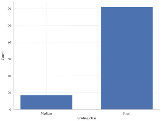
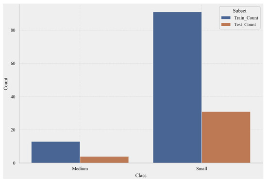
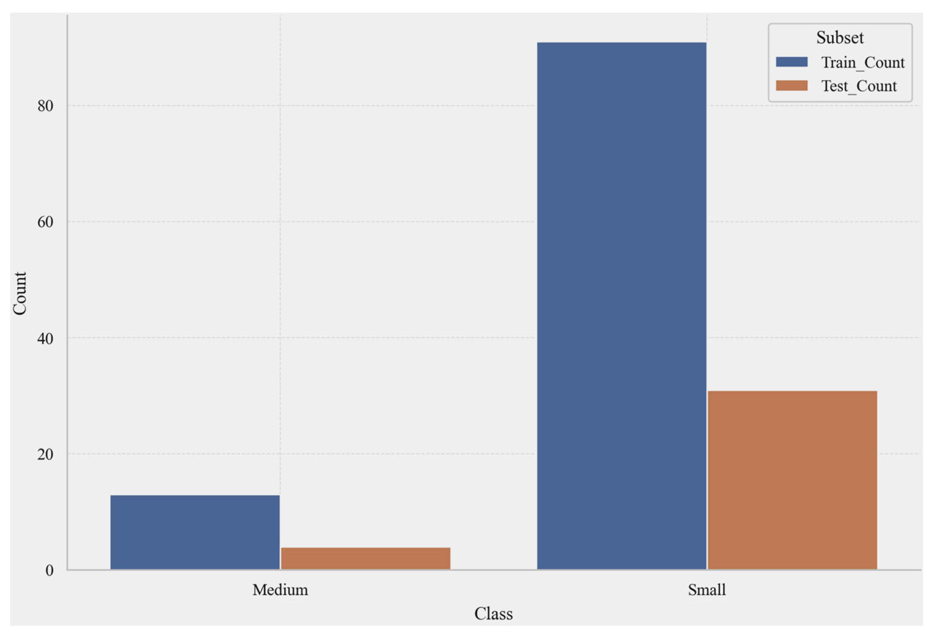
The seven variables characterize the features of erosion gullies across three dimensions: planimetric scale, longitudinal incision, and cross-sectional geometry. The dependent variable corresponds to the classification label. As presented in Table 2, the Small class constitutes 87.77% of the sample, while the Medium class comprises 12.23%.
Table 2.
Distribution of sample categories.
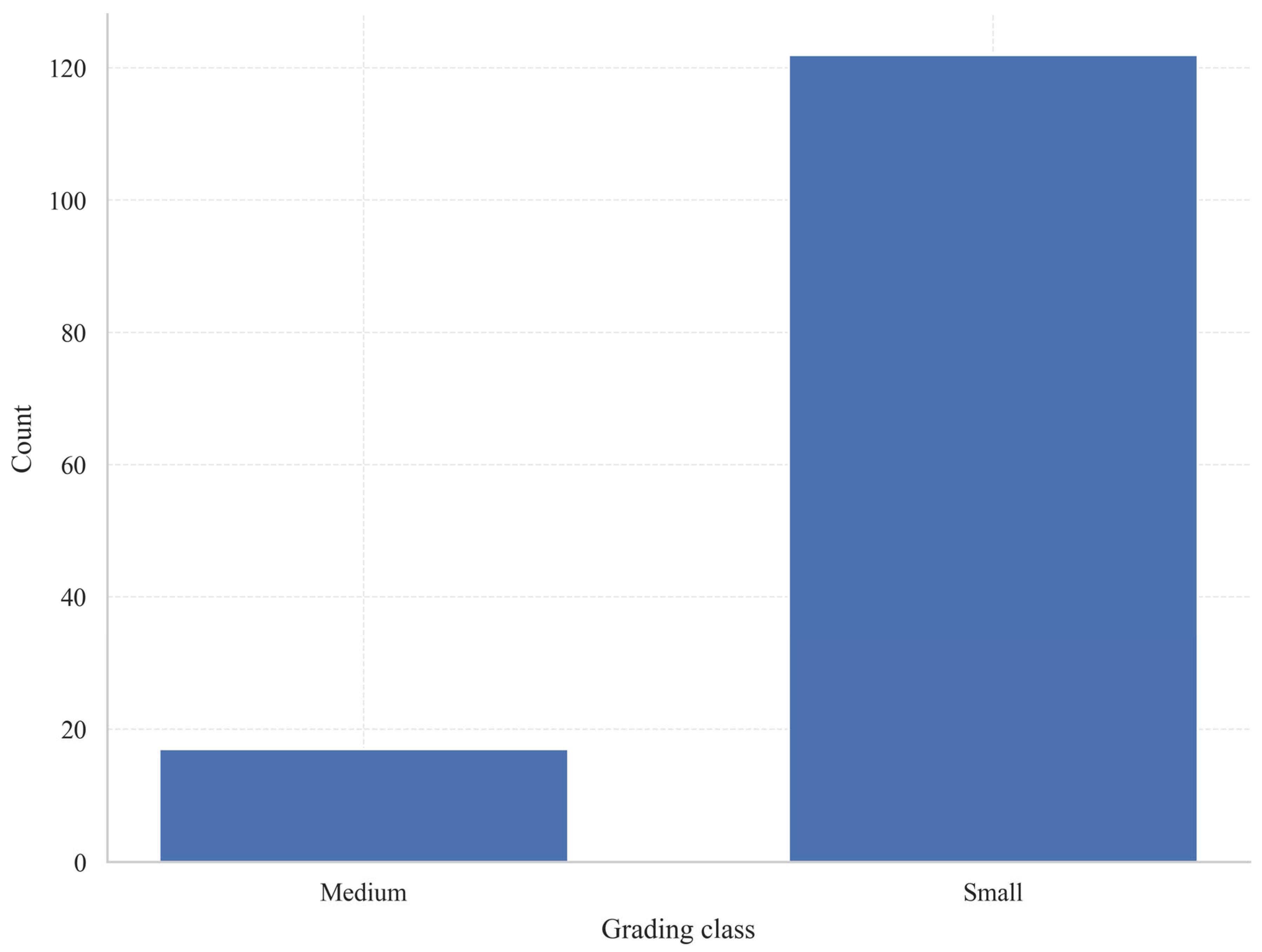
Figure 1 shows a highly imbalanced dataset, with the “Small” class constituting the overwhelming majority and the “Medium” class having relatively few samples. This structure explains why, despite the model’s high overall accuracy, special attention must still be paid to the recall and Macro-F1 performance of the “Medium” class.
Figure 1.
Distribution of erosion gully categories.
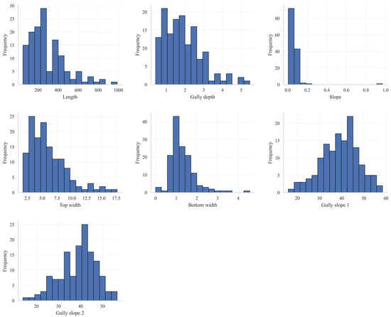
Figure 2 illustrates the frequency distribution characteristics of seven channel parameters measured across 139 erosion gullies. Generally, the majority of these parameters display skewed distributions, reflecting considerable variability among the samples. Gully lengths predominantly range from 100 to 400 m, with a minority extending beyond 800 m. Gully depths are mainly distributed between 1 and 3 m, indicating a predominance of shallow to moderately deep gullies. Gradient values are largely concentrated at the lower end of the spectrum, with only a few instances of relatively steep slopes, suggesting that the overall inclination of erosion gullies within the study area is relatively gentle. The top widths of the gullies are primarily between 3 and 8 m, whereas bottom widths mostly fall between 0.5 and 1.5 m, implying that the cross-sectional profiles typically exhibit a “wide at the top and narrow at the bottom” configuration. The slopes of the gully sides approximate a normal distribution, mainly ranging from 30° to 50°, with the second slope generally being slightly steeper than the first, indicating a degree of asymmetry in the morphological development of the gully walls. Collectively, these findings suggest that the erosion gullies in the study area are predominantly well-developed, characterized by moderate lengths, shallow depths, narrow bottoms, and relatively steep side slopes.
Figure 2.
Histograms of various characteristics.
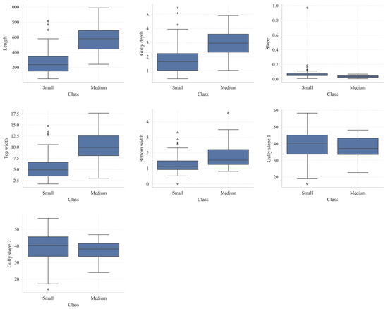
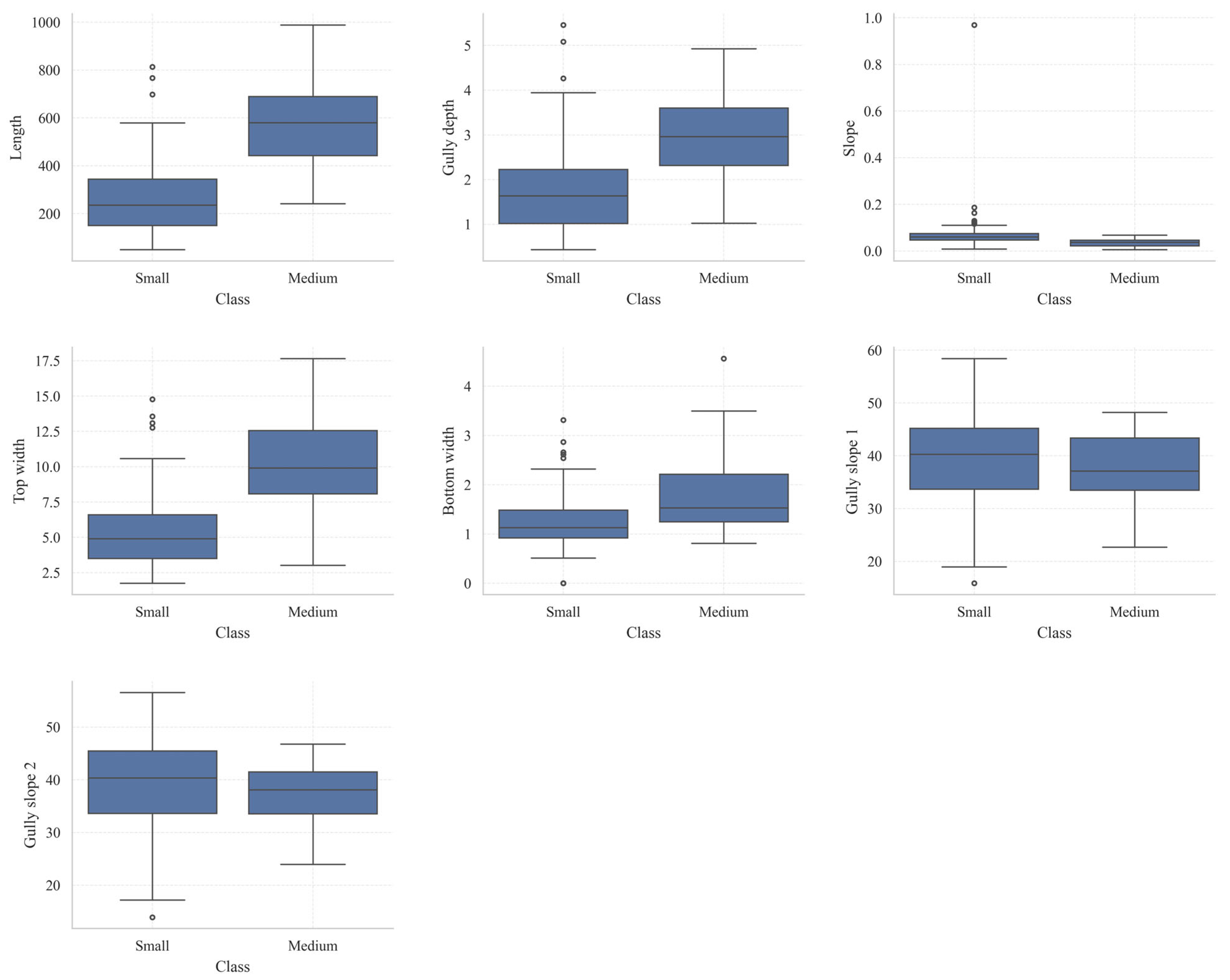
Figure 3 illustrates a comparative analysis of box-and-whisker plots depicting morphological parameters between small and medium-sized gullies. The median values for length, gully depth, top width, and bottom width are markedly greater in medium-sized gullies compared to small gullies, suggesting that as gully development progresses, the overall dimensions of the gully channel expand, with the most notable differences observed in length and top width. In terms of gradient, both categories of erosion gullies exhibit generally low values; however, small gullies demonstrate higher variability and a greater number of outliers, implying a stronger influence of local topographic conditions on some small gullies. Differences between Slope 1 and Slope 2 between the two gully types are minimal, with substantial overlap in the box plots, indicating that slope is a relatively insensitive parameter for differentiating stages of gully development. Nonetheless, the range of slope gradient variation is marginally broader for small gullies, whereas medium-sized gullies display a more concentrated distribution, reflecting a tendency toward morphological stabilization.
Figure 3.
Box-and-whisker plots of features grouped by grade.
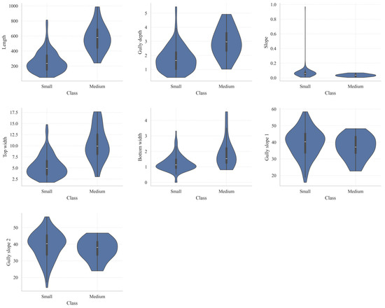
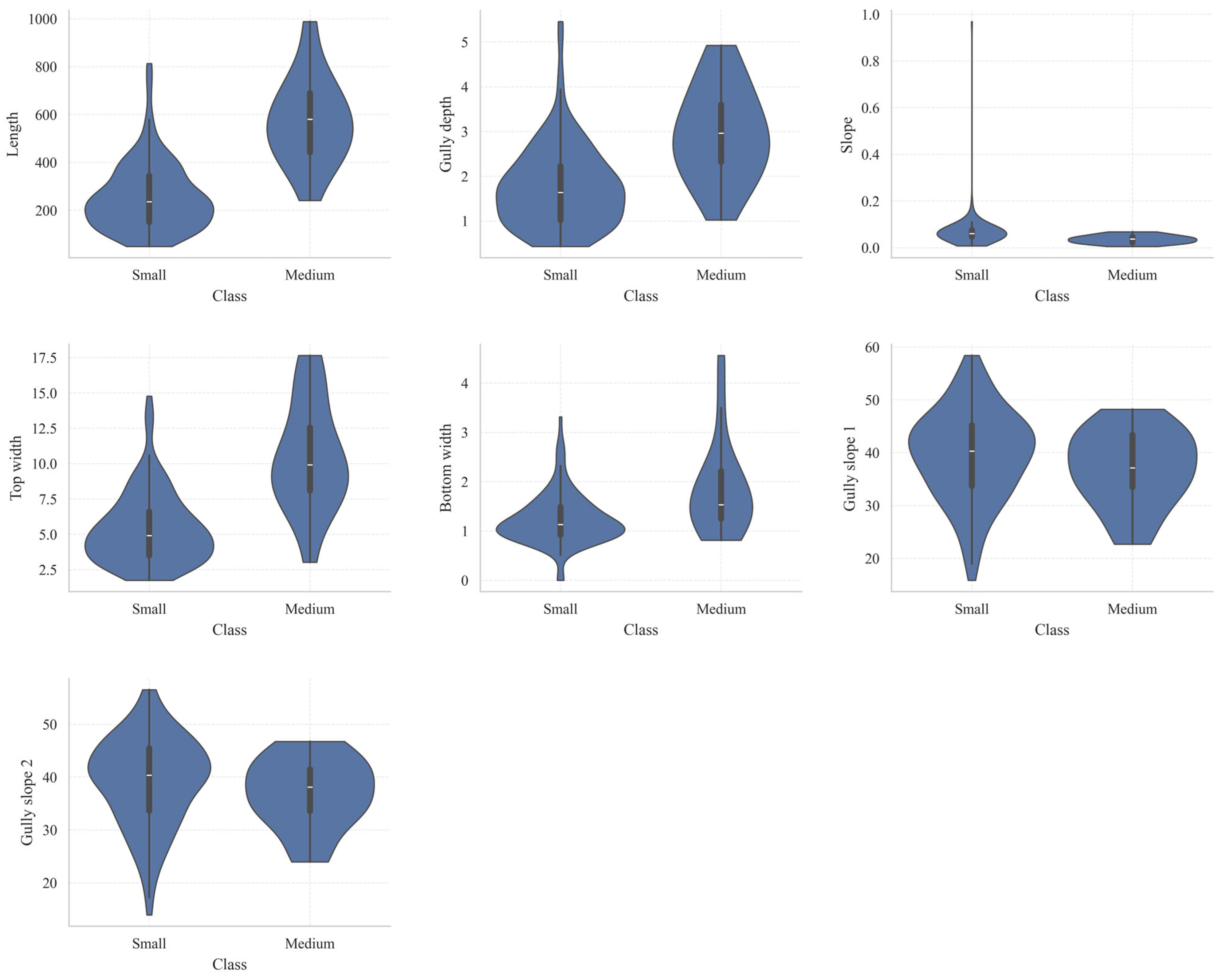
Figure 4 presents a violin plot to illustrate the differences in the distribution of morphological parameters between small and medium-sized gullies. This visualization not only highlights the median and interquartile range but also captures the density characteristics of the data. Generally, the distributions for medium-sized gullies in terms of length, gully depth, top width, and bottom width are shifted toward higher values, suggesting that as gully erosion progresses, the scale of the channels increases markedly. Notably, the differences are most pronounced in gully length and top width. The gradient values remain relatively low for both categories of gullies. Small gullies demonstrate a more dispersed distribution with a long tail extending toward higher values, implying a stronger influence of local topographic variability. In contrast, the slope angles of gully sides show minimal variation between small and medium-sized gullies, predominantly ranging from 30° to 45°. However, the distribution for small gullies is somewhat broader and more variable, whereas medium-sized gullies exhibit a more concentrated distribution, indicative of a comparatively stable morphological structure.
Figure 4.
Scatter plots of various characteristics grouped by grade.
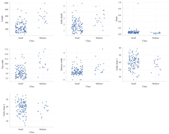
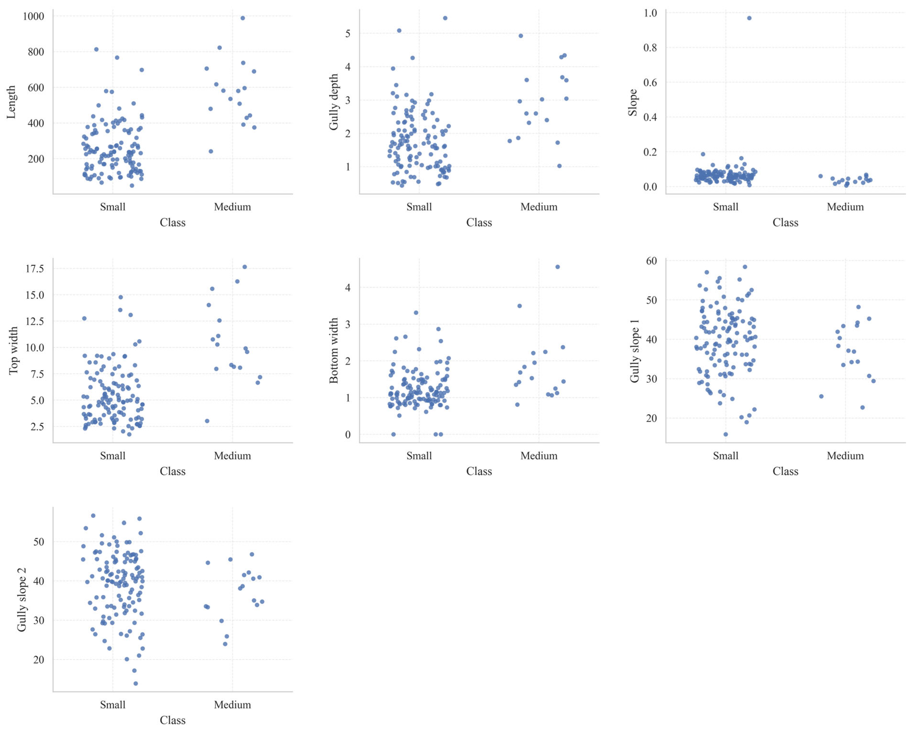
Figure 5 shows the clustered scatter plots of various characteristic parameters for erosion gullies of different grades. Overall, the number of small gully samples is significantly higher than that of medium-sized gullies, and the distribution of various indicators is more dispersed, indicating greater morphological variation and differing stages of development; medium-sized gully samples are relatively fewer, but their overall distribution for indicators such as length, gully depth, top width, and bottom width falls within a higher value range, reflecting that as gully development progresses, trends toward channel extension, downcutting, and widening become more pronounced. Specifically, the lengths of small gullies are mostly concentrated between 100 and 400 m, with depths typically ranging from 1 to 3 m; crest widths are primarily distributed between 3 and 8 m, while base widths are mostly between 0.8 and 1.8 m. In contrast, medium-sized gullies generally exhibit larger values for these parameters, with some samples reaching lengths close to 1000 m and crest widths exceeding 15 m, indicating a more advanced stage of erosion development. The gradient was generally low in both types of erosion gullies, but it fluctuated more significantly in small gullies and exhibited extreme high values, indicating that local topographic conditions had a more pronounced influence on them.
Figure 5.
Scatter-strip plot of features grouped by grade.
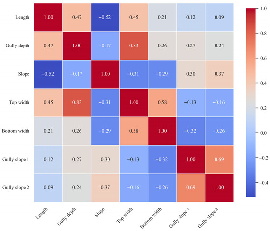
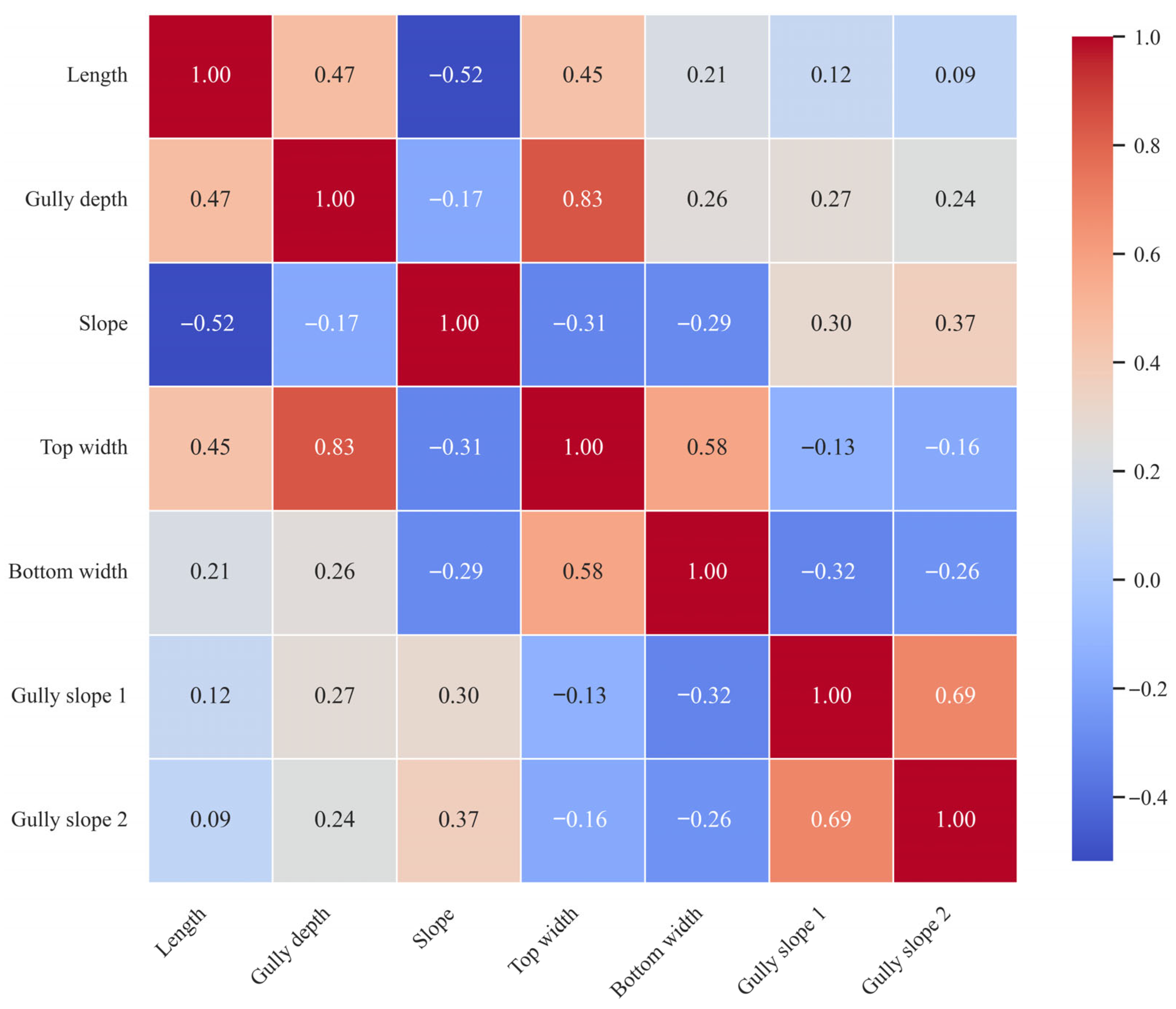
Figure 6 shows a Spearman correlation heatmap for the morphological parameters of each gully, illustrating the strength and direction of the monotonic correlations between variables. Overall, the correlation between gully depth and crest width is the strongest (r = 0.83), indicating that as a gully becomes deeper, its crest tends to widen more significantly, suggesting a strong synergistic developmental relationship between the two. Gully slope 1 and gully slope 2 also exhibit a strong positive correlation (r = 0.69), indicating that changes in slope on both sides of the gully are highly consistent. Channel length shows a moderate positive correlation with both channel depth (r = 0.47) and top width (r = 0.45), indicating that as the channel develops, an increase in length is typically accompanied by a deepening of the channel body and a widening of the top. A certain positive correlation is also observed between top width and bottom width (r = 0.58), reflecting an overall expansion trend in the channel cross-section. In contrast, the gradient showed a negative correlation with most indicators, particularly with gully length (r = −0.52), top width (r = −0.31), and bottom width (r = −0.29). This indicates that as the gradient increases, the overall scale of the gully tends to decrease, suggesting that in steep slope sections, gully development is still primarily in the initial cutting stage and has not yet fully expanded. Furthermore, the correlation between gully slope and gully length or width is generally weak, suggesting that slope gradient has a limited direct influence on gully scale.
Figure 6.
Spearman correlation heatmap.
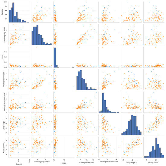
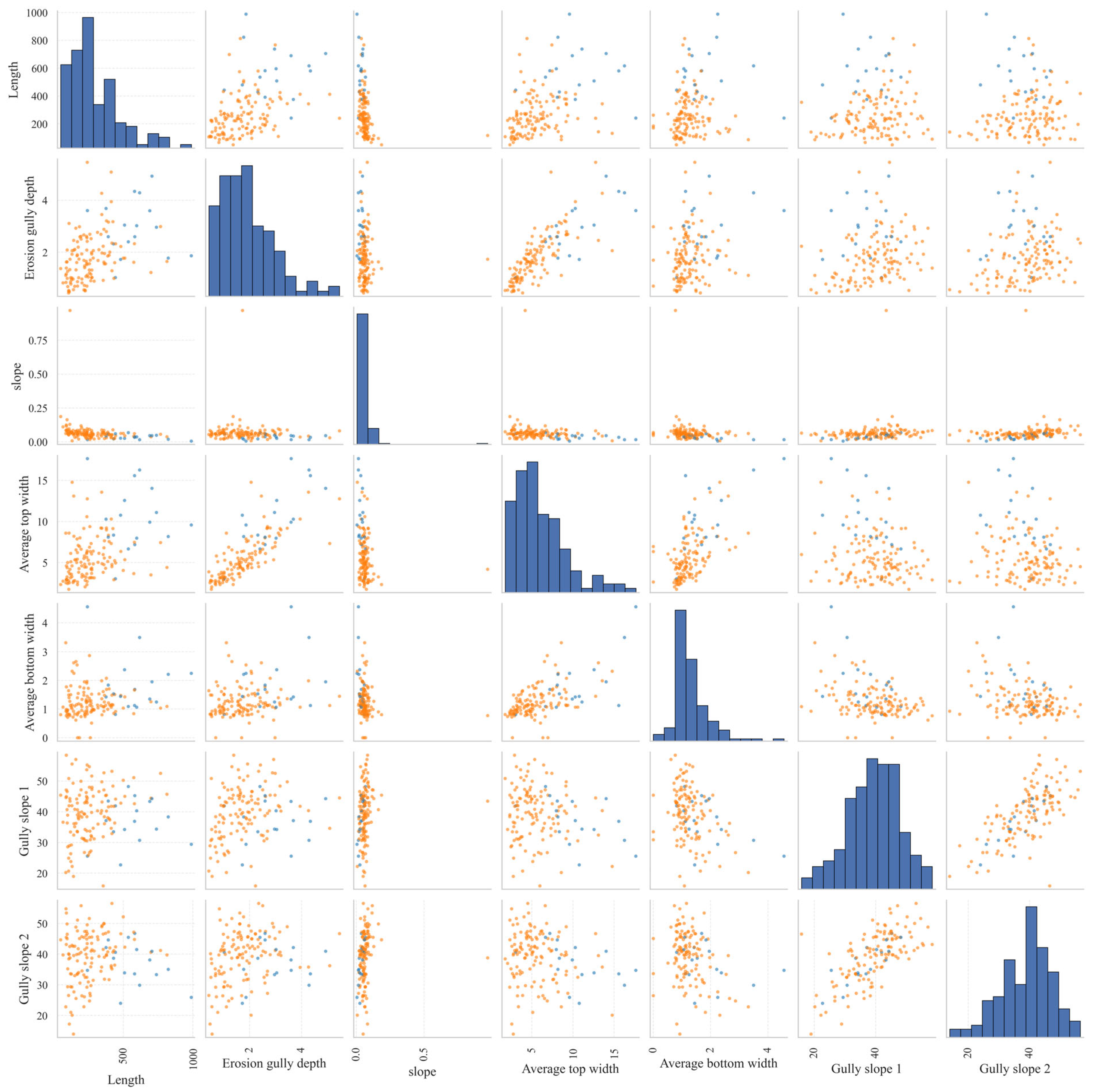
Figure 7 shows a scatter plot of the morphological parameters of each gully. The diagonal positions display the distribution characteristics of each indicator, while the off-diagonal positions reflect the correlations between pairs of parameters. Different colors are used to distinguish between different grades of erosion gullies. Length, gully depth, average top width, and average bottom width all exhibit a distinct right-skewed distribution, with most samples concentrated within a narrow range of values and a few samples exhibiting larger values. This indicates that erosion gullies in the study area are predominantly of small to medium scale, though some more extensively developed gullies are present. The scatter plot reveals a strong positive correlation between gully depth and average top width, as well as a certain positive correlation between gully length and both gully depth and top width. This indicates that during their development, erosion gullies tend to simultaneously increase in length along the channel, deepen downward, and widen laterally. The average crown width and average base width also exhibit a certain degree of coordinated variation, indicating that the expansion of the gully cross-section is holistic. In contrast, the correlation between gradient and gully length, depth, and width is weak or even shows a certain degree of negative correlation, suggesting that an increase in slope gradient does not necessarily correspond to larger-scale erosion gullies. The slopes on both sides of the gullies are primarily concentrated between 30° and 50°, and the distributions of Slope 1 and Slope 2 are similar, with a strong correlation, indicating a high degree of consistency in the morphology of both sides of the gully slopes. Although there is some overlap among samples of different grades, medium-sized gullies are generally more distributed in the high-value regions, reflecting that their developmental stage is higher than that of small gullies.
Figure 7.
Feature scatter matrix.
2.2. Descriptive Statistics and Variable Relationships
Table 3, which summarizes the descriptive statistics, reveals substantial variability in the geometric parameters of the erosion gullies. The maximum recorded Length approaches 1000, indicating the presence of gullies with markedly diverse scales within the sample. The maximum Average top width is 17.649, considerably exceeding the maximum Average bottom width of 4.560, implying that the majority of erosion gully cross-sections are characterized by a wider top and a narrower bottom. Notable differences in both magnitude and dispersion are observed among the variables. Specifically, Length, erosion gully depth, and Average top width demonstrate greater variability, suggesting that erosion gullies at various developmental stages can be effectively differentiated based on their morphological features.
Table 3.
Descriptive statistics of key variables.
2.3. Technical Approach and Modeling Process
First, the raw data underwent field standardization and missing value checks; since none of the 139 samples in this batch had missing features, the number of valid samples remained unchanged. Second, based on the seven basic morphological indicators, a set of interaction terms with clear geomorphological significance was constructed, including Length × slope, Length × Erosion gully depth, Erosion gully depth × Average top width, Erosion gully depth × Average bottom width, Average top width × Slope, and Average bottom width × Slope, to characterize the combined effects of longitudinal scale, incision capacity, lateral widening, and slope energy. Next, correlation filtering and VIF (variance inflation factor) diagnostics were performed on the basic variables and interaction terms. The final set of 8 retained variables are Length, Average top width, slope, Length × slope, Length × Erosion gully depth, Erosion gully depth × Average top width, Erosion gully depth × Average bottom width, and Average bottom width × slope. It should be emphasized that this result implies that, under the current sample conditions, retaining only the original univariate variables might compromise the ability to capture the coupled mechanisms of gully development.
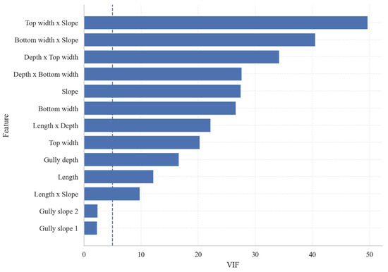
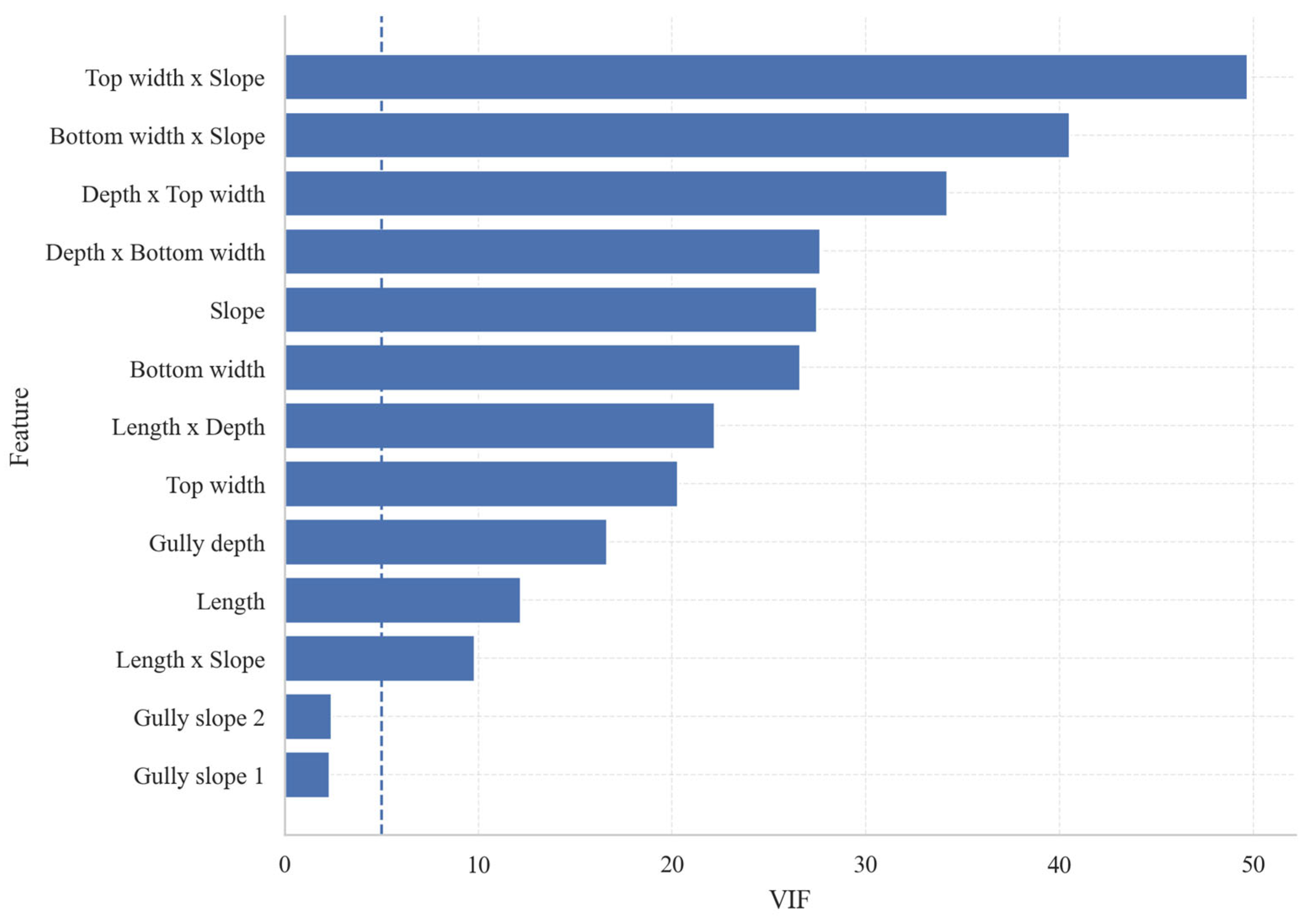
Figure 8 presents the results of the Variance Inflation Factor (VIF) test for each candidate variable, used to identify the degree of multicollinearity among features. Overall, the VIF values for most interaction terms in the figure are significantly higher than the commonly used threshold of 5 indicated by the dashed line, indicating strong correlations among these variables. Among them, Top width × Slope has the highest VIF, approaching 50, indicating the most severe information overlap with other variables; The VIF values for Bottom width × Slope, Depth × Top width, and Depth × Bottom width are also at relatively high levels, reflecting significant coupling relationships among slope, gully depth, and gully rim width. At the same time, although the VIFs for Slope, Bottom width, Length × Depth, Top width, Gully depth, and Length vary, they are generally still above or close to the warning threshold, indicating a certain degree of information redundancy between the original morphological indicators and the structural interaction terms. In contrast, the VIF for Length × Slope is close to the threshold and on the borderline of acceptability, while Gully slope 1 and Gully slope 2 are significantly below the threshold, indicating weak multicollinearity.
Figure 8.
Variance Inflation Factor (VIF) analysis of basic variables and interaction terms.
This research employed Random Forest (RF) as the primary modeling approach and conducted comparative analyses against Logistic Regression, Support Vector Machines (SVM), Decision Trees, and Backpropagation Neural Networks (BPNN) as benchmark models. Random Forest represents a prototypical ensemble learning technique applicable to both classification and regression problems. Its core mechanism involves enhancing predictive accuracy, generalization performance, and mitigating overfitting by aggregating the classification outcomes of multiple decision trees [19]. Specifically, during the training phase, Random Forest utilizes the Bootstrap sampling method to generate multiple independent training subsets through repeated sampling with replacement from the original dataset. Furthermore, at each decision tree node, rather than considering the entire feature set, a randomly selected subset of features is employed to determine the optimal split. This strategy increases the heterogeneity among base learners and diminishes the model’s dependence on any single sample distribution or feature combination. In classification scenarios, the final class assignment for a given sample is determined via majority voting across all trees, whereas in regression tasks, the predicted value is derived by averaging the outputs of the individual trees. Given its robust nonlinear modeling capacity, resilience to noise, and interpretability, Random Forest was deemed an appropriate primary model for the classification of erosion gullies in this study.
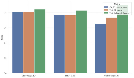
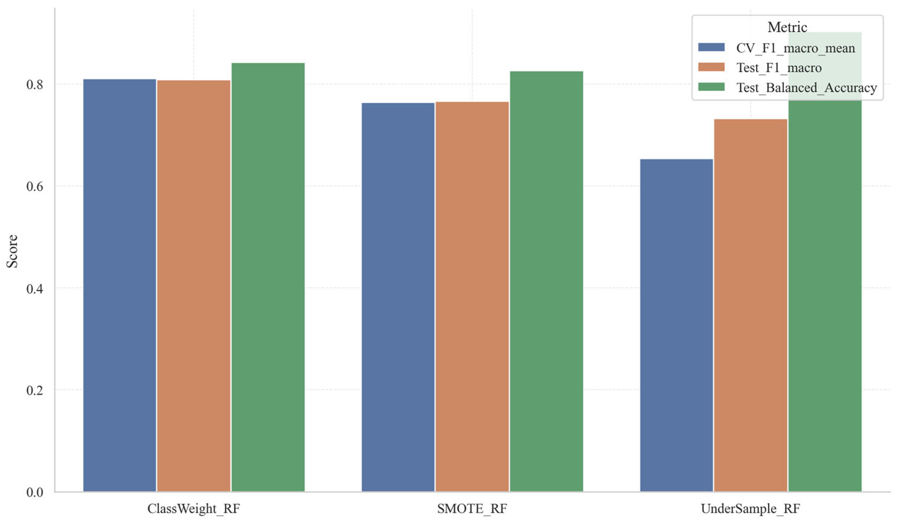
During the modeling phase, this study utilizes a stratified random sampling technique to partition the entire dataset into training and test subsets at a ratio of 75% to 25%, thereby preserving the proportional representation of categories in both subsets consistent with the overall sample distribution (see Figure 9). For the training subset, hyperparameter optimization of the Random Forest model was conducted through a grid search procedure, yielding the optimal parameter set: n_estimators = 400, max_depth = 4, min_samples_split = 14, min_samples_leaf = 4, and max_features = sqrt. This configuration suggests that by regulating tree depth and leaf node size while moderately increasing the number of base learners, the study enhances ensemble performance, achieving an optimal trade-off between model complexity and generalization capability. Furthermore, to address the issue of class imbalance and its potential adverse effects on classification outcomes, the Random Forest model incorporated a class weight balancing strategy (class_weight = balanced) during training. Figure 10 presents a comparative analysis of three class imbalance handling approaches within the Random Forest framework: ClassWeight_RF, SMOTE_RF, and UnderSample_RF. Overall, ClassWeight_RF exhibits superior comprehensive performance, as evidenced by its high cross-validation F1-macro score, test set F1-macro score, and test set Balanced Accuracy. These results indicate that adjusting class weights effectively enhances minority class recognition while maintaining model stability. SMOTE_RF ranks second in overall performance, with metrics marginally lower than those of ClassWeight_RF, suggesting that synthetic minority sample generation positively influences model performance, albeit with limited improvement. Conversely, UnderSample_RF demonstrates a substantially lower cross-validation F1-macro score. Although its test set F1-macro and Balanced Accuracy show some gains, its overall stability is compromised, implying that undersampling may diminish training efficacy due to the loss of information from the majority class. In summary, given the current context of limited sample size and class imbalance, the class weighting approach emerges as a more appropriate balancing strategy for Random Forest models compared to oversampling and undersampling techniques.
Figure 9.
Category distribution of training and test sets.
Figure 10.
Comparison of random forest classification performance under different sample balancing strategies.
To strengthen the reliability of the findings, this study refrained from assessing model performance based solely on a single training–test split. Instead, a consistent application of grid search and hierarchical cross-validation was employed across all candidate models during the training phase, with the F1-macro score designated as the principal evaluation metric. The choice of F1-macro was motivated by the presence of class imbalance within the dataset, as this metric equally weights all classes, thereby providing a more balanced assessment of the model’s overall recognition performance across both minority and majority classes. Ultimately, the Random Forest model was determined to be the most effective for this study, upon which subsequent analyses—including threshold optimization, error diagnosis, and interpretability evaluation—were conducted.
2.4. SHAP Explanation Framework
The ‘shap.TreeExplainer’ is a specialized interpretability tool within the SHAP framework, explicitly developed for tree-based models such as Random Forest, XGBoost, LightGBM, and CatBoost [36]. Grounded in Shapley value theory, it decomposes the prediction of a model for an individual instance into additive contributions from each feature, thereby quantifying the extent to which each variable positively or negatively influences the prediction. Unlike general SHAP approaches, TreeExplainer exploits the inherent structural properties of tree models, ensuring both consistency and local accuracy in its explanations while substantially enhancing computational efficiency. This makes it particularly well-suited for interpreting complex tree-based algorithms. In practical applications, ‘shap.TreeExplainer’ facilitates the computation of SHAP values for individual features at the single-sample level, enabling detailed explanations of why a model assigns a particular classification to that instance. Additionally, it can calculate the mean absolute SHAP values across the dataset to evaluate the overall importance of each feature. At the global interpretability level, visualization techniques such as summary plots, beeswarm plots, and bar charts are commonly employed to depict feature importance and illustrate the relationship between feature values and their directional contributions. At the local level, waterfall and force plots are utilized to elucidate the specific predictive rationale for representative samples. Consequently, ‘shap.TreeExplainer’ effectively transforms opaque tree-based models into transparent frameworks of feature contributions, offering essential insights for understanding variable mechanisms, validating model reliability, and supporting the interpretation of predictive outcomes.
3. Result Analysis
3.1. Model Selection Results and Overall Performance
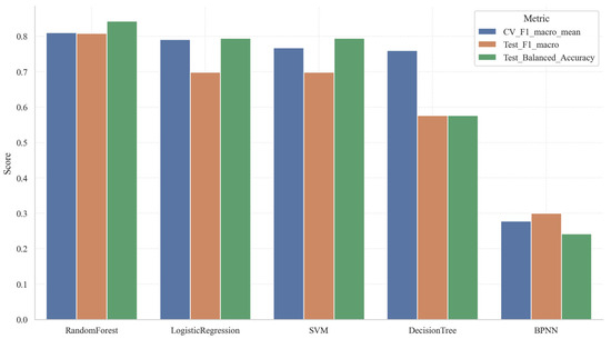
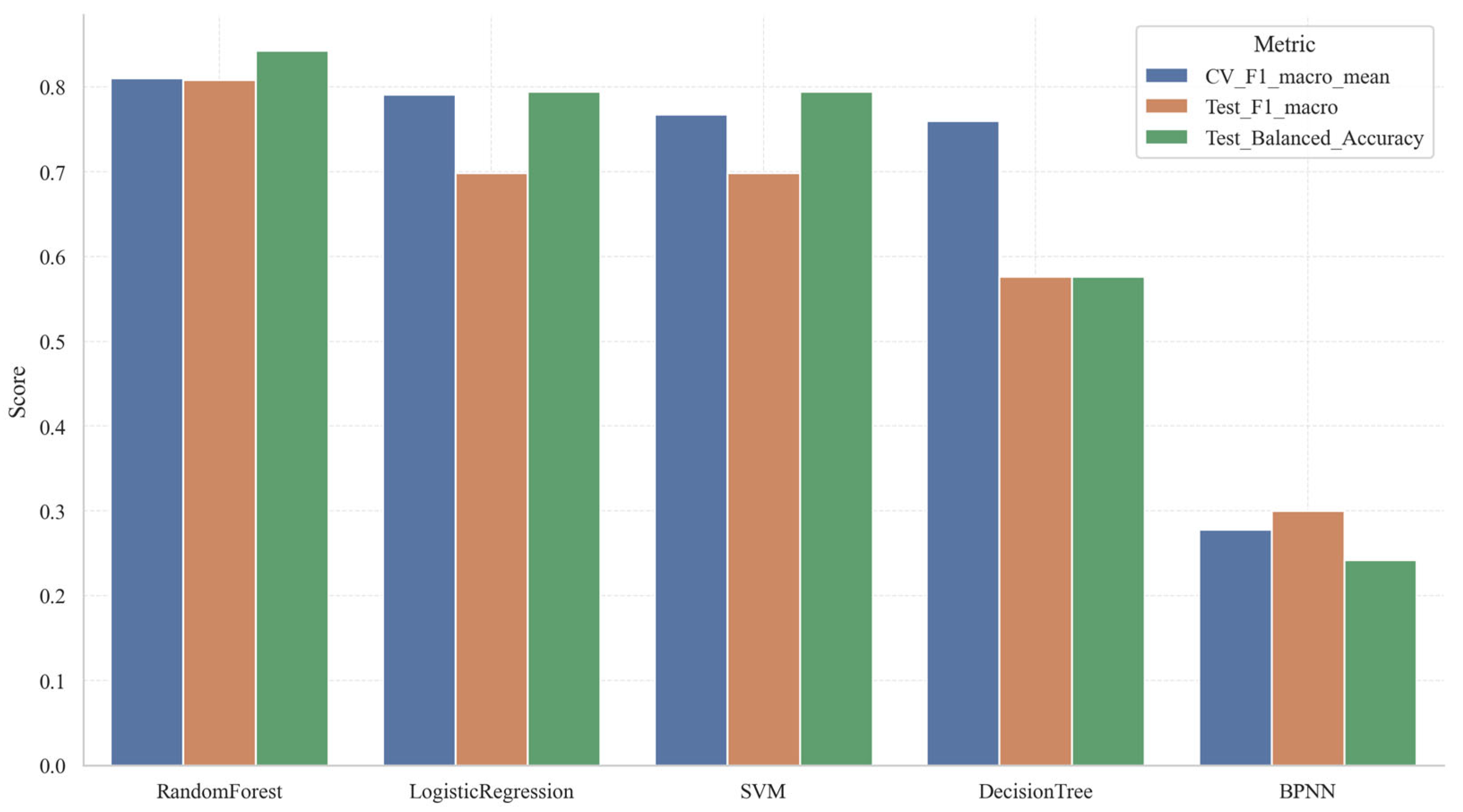
An integrated analysis of Table 4 and Figure 11 elucidates distinct hierarchical distinctions among the five candidate models with respect to cross-validation outcomes, test set performance, and aggregate scoring metrics. The Random Forest model exhibits superior overall performance, evidenced by a mean cross-validation F1 score of 0.8105, a test F1-macro score of 0.8087, a test Balanced Accuracy of 0.8427, and a test Accuracy of 0.9143. Additionally, it attains the highest composite score of 0.7953. These results suggest that the Random Forest model not only demonstrates robust multi-class classification capabilities but also maintains stability in the presence of class distribution imbalances. Logistic Regression and Support Vector Machine (SVM) models constitute the second tier of performance. Both models achieve a test F1-macro score of 0.6983, a Balanced Accuracy of 0.7944, and a test Accuracy of 0.8286. However, Logistic Regression slightly outperforms SVM, with a mean cross-validation F1 score of 0.7908 and a composite score of 0.7289, compared to SVM’s 0.7679 and 0.7176, respectively. This indicates a marginally superior overall performance for Logistic Regression. It is noteworthy that although the generalization gaps for these models are relatively small (0.0596 for Logistic Regression and 0.0681 for SVM), indicating acceptable generalization capabilities, their cross-validation standard deviations are comparatively high (0.2126 and 0.2152, respectively). This suggests sensitivity to variations in sample partitioning across different folds. The Decision Tree model presents a mean cross-validation F1 score of 0.7601, which is moderate; however, it exhibits a substantial generalization gap of 0.1992. Correspondingly, its test F1-macro and Balanced Accuracy scores decline to 0.5766, indicative of pronounced overfitting. Conversely, the Backpropagation Neural Network (BPNN) demonstrates markedly inferior performance across all metrics, with a composite score of merely 0.2678. This outcome implies that, given the limited dataset size of 139 samples, the model’s complex nonlinear architecture does not confer a significant advantage. In summary, the Random Forest model achieves the most favorable balance among accuracy, robustness, and generalization ability, and is therefore recommended as the optimal model for the present study.
Table 4.
Comparison results of candidate models.
Figure 11.
Comparison of overall performance among candidate models.
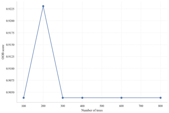
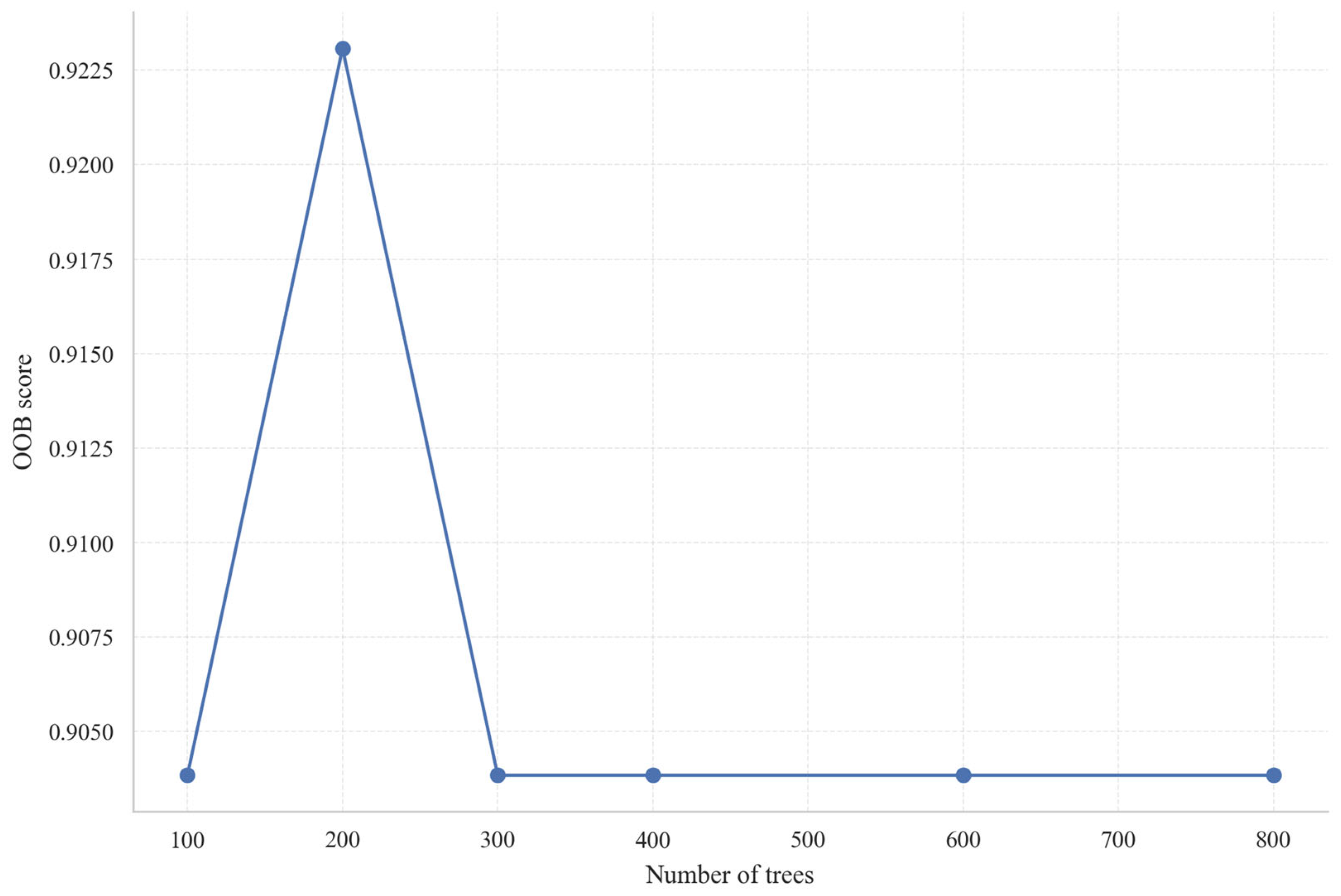
Figure 12 depicts the relationship between the number of trees in the Random Forest model and the corresponding out-of-bag (OOB) score. According to the results obtained from the single-factor variation analysis, increasing the number of trees from 100 to 200 leads to an improvement in the OOB score from approximately 0.904 to 0.923, reaching a local optimum. However, further increases in the number of trees to 300, 400, 600, and 800 result in the OOB score stabilizing around 0.904, suggesting that, based solely on the OOB curve, 200 trees provide the best out-of-bag performance, with additional trees offering negligible improvement. Nevertheless, the present study did not rely exclusively on OOB score variations of a single parameter for model selection. Instead, a grid search was conducted on the training dataset to jointly optimize multiple hyperparameters, including n_estimators, max_depth, min_samples_split, min_samples_leaf, and max_features. The optimal parameter set identified comprises n_estimators = 400, max_depth = 4, min_samples_split = 14, min_samples_leaf = 4, and max_features = sqrt. This finding indicates that although 200 trees yielded a higher OOB score when considered in isolation, the configuration with 400 trees—combined with constraints on tree depth and node splitting criteria—achieves a superior balance among model complexity, generalization capability, and stability.
Figure 12.
Random Forest OOB convergence curve.
3.2. Classification Performance
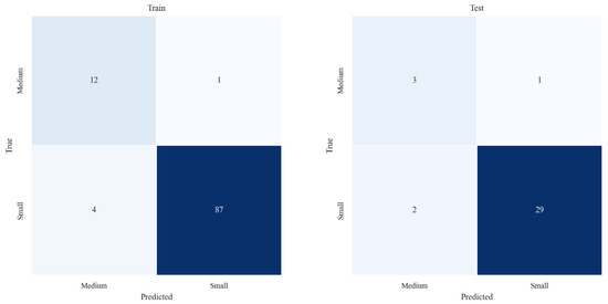
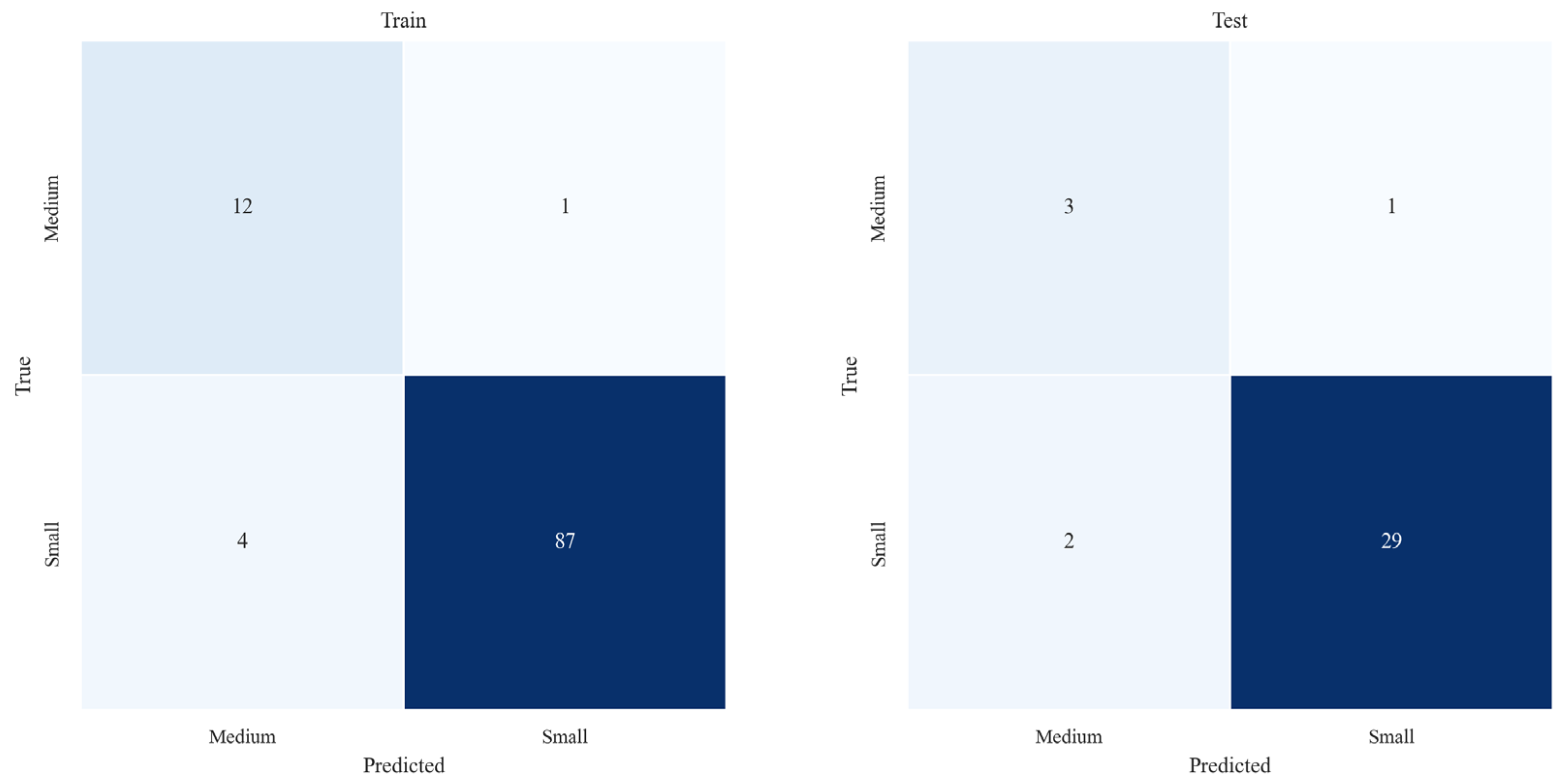
As presented in Table 5, which summarizes the classification results on the comprehensive test set, and illustrated by the confusion matrix in Figure 13, the Random Forest model exhibits robust overall recognition ability and relatively balanced discrimination across classes in the current gully classification task. The test set comprises 35 samples, of which 32 were accurately classified, yielding an overall accuracy of 0.9143. The macro-averaged Precision, Recall, and F1-score were 0.7833, 0.8427, and 0.8087, respectively, indicating that the model sustained strong performance despite the presence of class imbalance. Examination of the confusion matrix reveals that 3 out of 4 Medium class samples were correctly identified, with one misclassified as Small, resulting in a Recall of 0.7500 for the Medium class. Concurrently, the model accurately classified 29 out of 31 Small class samples, with only 2 misclassified as Medium, corresponding to Precision, Recall, and F1-score values of 0.9667, 0.9355, and 0.9508, respectively, for the Small class, thereby demonstrating highly consistent performance. For the Medium class, the Precision and F1-score were 0.6000 and 0.6667, respectively. Although these metrics are lower than those observed for the Small class, the model successfully identified the majority of Medium samples despite the limited sample size in this category, suggesting that the model possesses a notable capacity for detecting critical target classes.
Table 5.
Classification results on the test set.
Figure 13.
Confusion matrix for the Random Forest training and test sets.
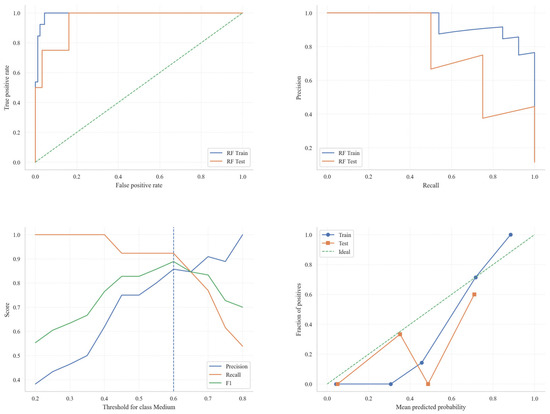
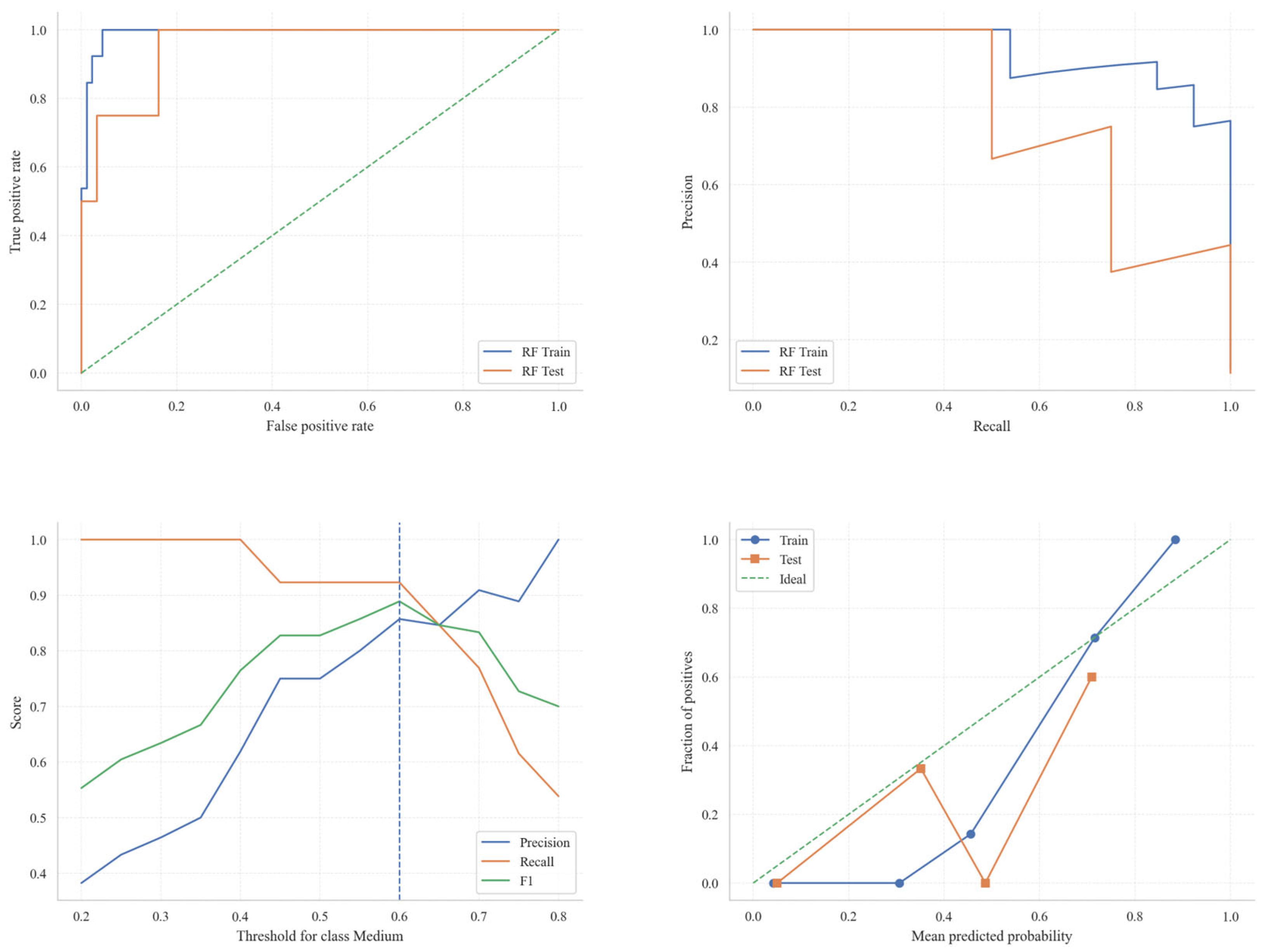
Figure 14 provides a comprehensive evaluation of the Random Forest model’s performance on both the training and test datasets, comprising four distinct subplots: the Receiver Operating Characteristic (ROC) curve, the Precision–Recall curve, the variation of Precision, Recall, and F1-score with respect to the classification threshold, and the association between predicted probabilities and the proportion of positive instances. The ROC curve (top left) depicts the model’s discriminative ability on the training and test sets. The curve corresponding to the training data (blue) closely parallels that of the test data (orange), with both curves substantially exceeding the diagonal baseline indicative of random classification. This suggests that the model exhibits robust classification performance. The Precision–Recall curve (top right) further highlights the model’s capacity to maintain high recall for the Medium class. Notably, on the test set, precision decreases at elevated recall levels, implying that the model adopts a conservative approach when identifying minority class instances, thereby accommodating the inherent class imbalance. The third subplot illustrates how Precision, Recall, and F1-score for the Medium class vary as the decision threshold changes. At a threshold value of 0.6, the model attains an optimal balance between precision and recall, with the F1-score approaching its peak, indicating that this threshold effectively mediates the trade-off between these metrics. Lastly, the bottom right graph examines the relationship between the predicted probabilities and the observed proportion of positive examples. The distribution of predicted probabilities on the test set deviates markedly from the idealized linear relationship, suggesting that positive predictions are dispersed, with some positive samples assigned relatively low probabilities. Nevertheless, an increasing trend is observed whereby higher predicted probabilities correspond to a greater proportion of positive instances.
Figure 14.
ROC, Precision–Recall, and Threshold Optimization analysis of the Random Forest model.
3.3. Algorithm Stability Analysis
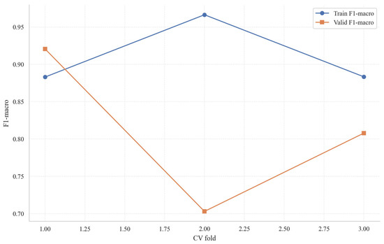
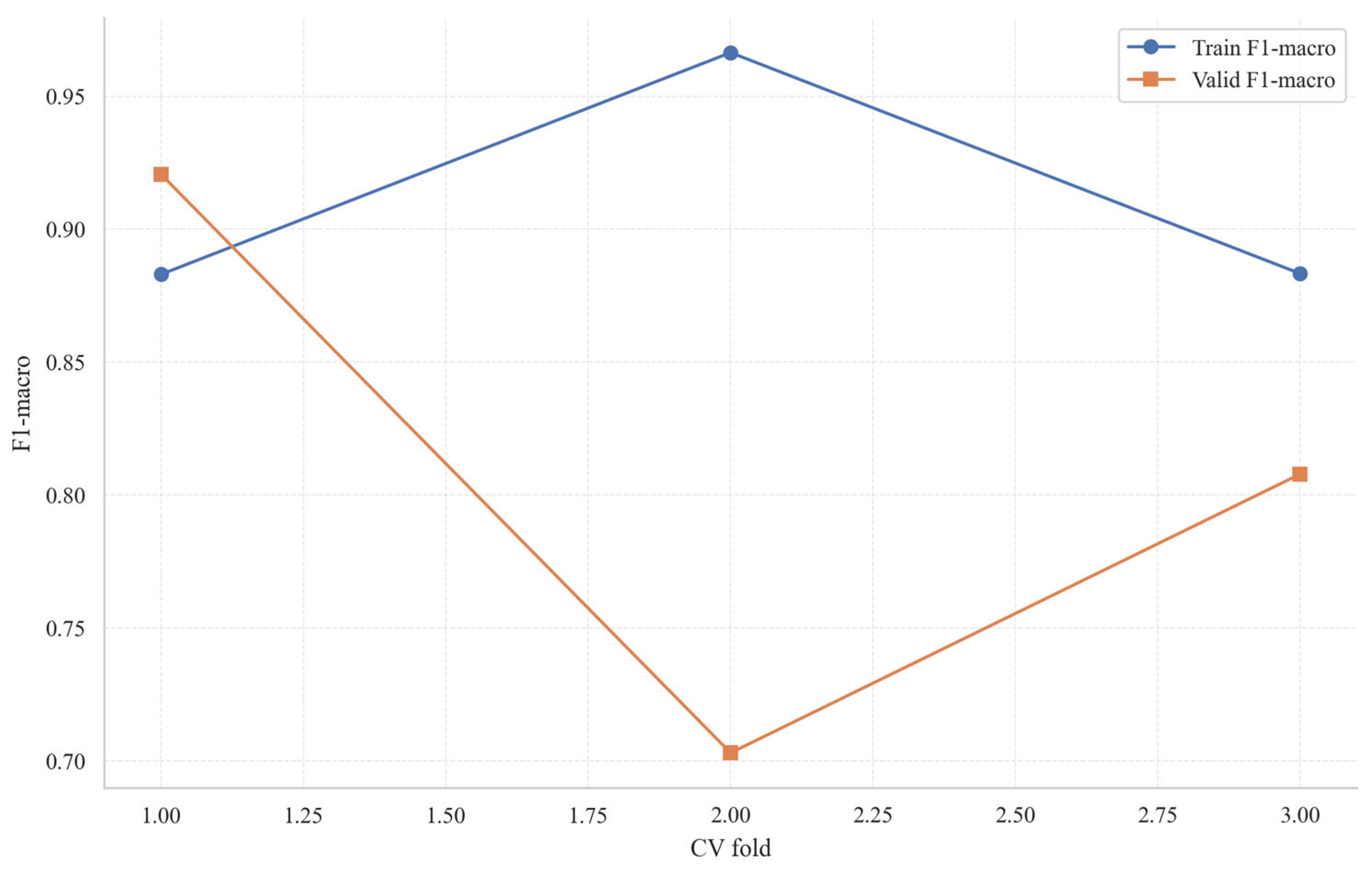
Figure 15 illustrates the outcomes of a single three-fold cross-validation procedure. The F1-macro scores obtained from the validation sets of the Random Forest model across the three folds were 0.9206, 0.7030, and 0.8079, respectively. The average F1-macro score was 0.8105, with a standard deviation of 0.1088. A marked discrepancy between the second and third folds is evident, suggesting that the model’s performance varies when samples from minority classes are allocated differently among the folds.
Figure 15.
Comparison of F1-macro scores for training and validation in each fold of the Random Forest.
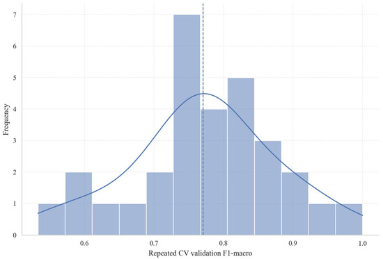
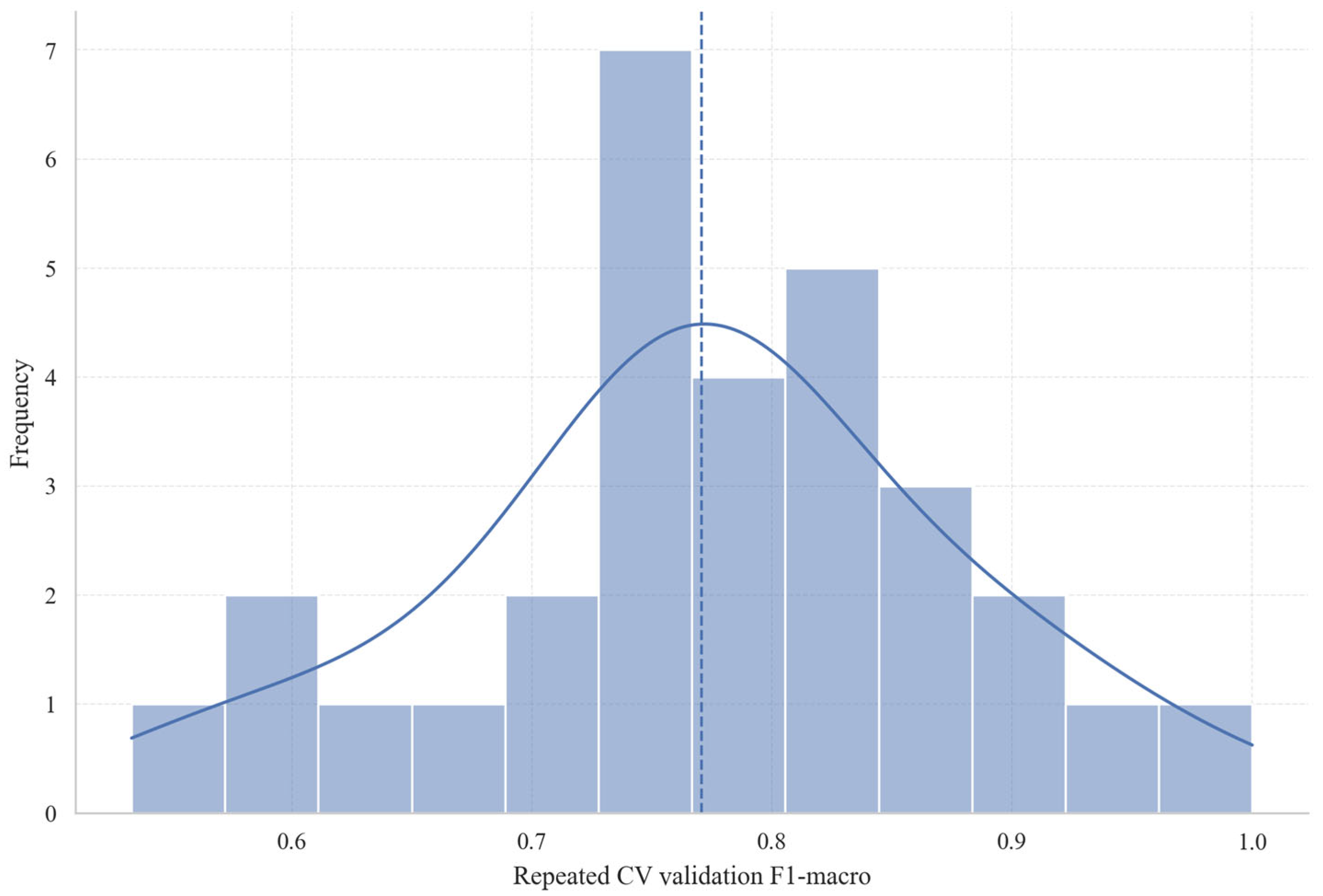
Figure 16 illustrates the distribution of F1-macro scores obtained from the Random Forest model over multiple iterations of cross-validation, thereby highlighting the consistency of the model’s performance across various validation folds. The histogram and the superimposed density curve reveal that the majority of F1-macro scores are concentrated within the range of 0.7 to 0.85, approximating a normal distribution. Performance metrics predominantly cluster in the higher score interval, with the most frequent scores falling between 0.75 and 0.8, suggesting that the model maintains a stable level of performance throughout repeated cross-validation. The blue dashed line denotes the mean F1-macro score, positioned near 0.80, which indicates a relatively balanced and robust classification performance across the validation process. Given that this average exceeds 0.7, it signifies strong predictive capability. Although certain validation folds yielded lower F1-macro scores, approaching 0.6, the overall pattern underscores the Random Forest model’s robustness and reproducibility, demonstrating its effective generalization across different data partitions.
Figure 16.
F1 distribution of the validation set under repeated hierarchical cross-validation.
4. Feature Importance and Interpretability Analysis
4.1. Comparison of Three Types of Importance Metrics
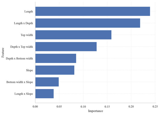
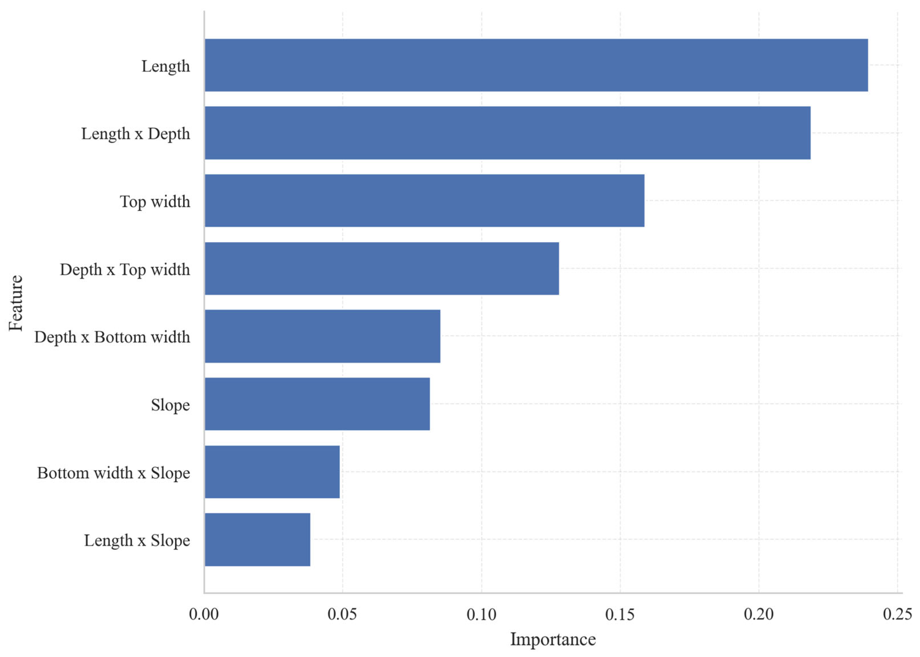
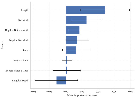
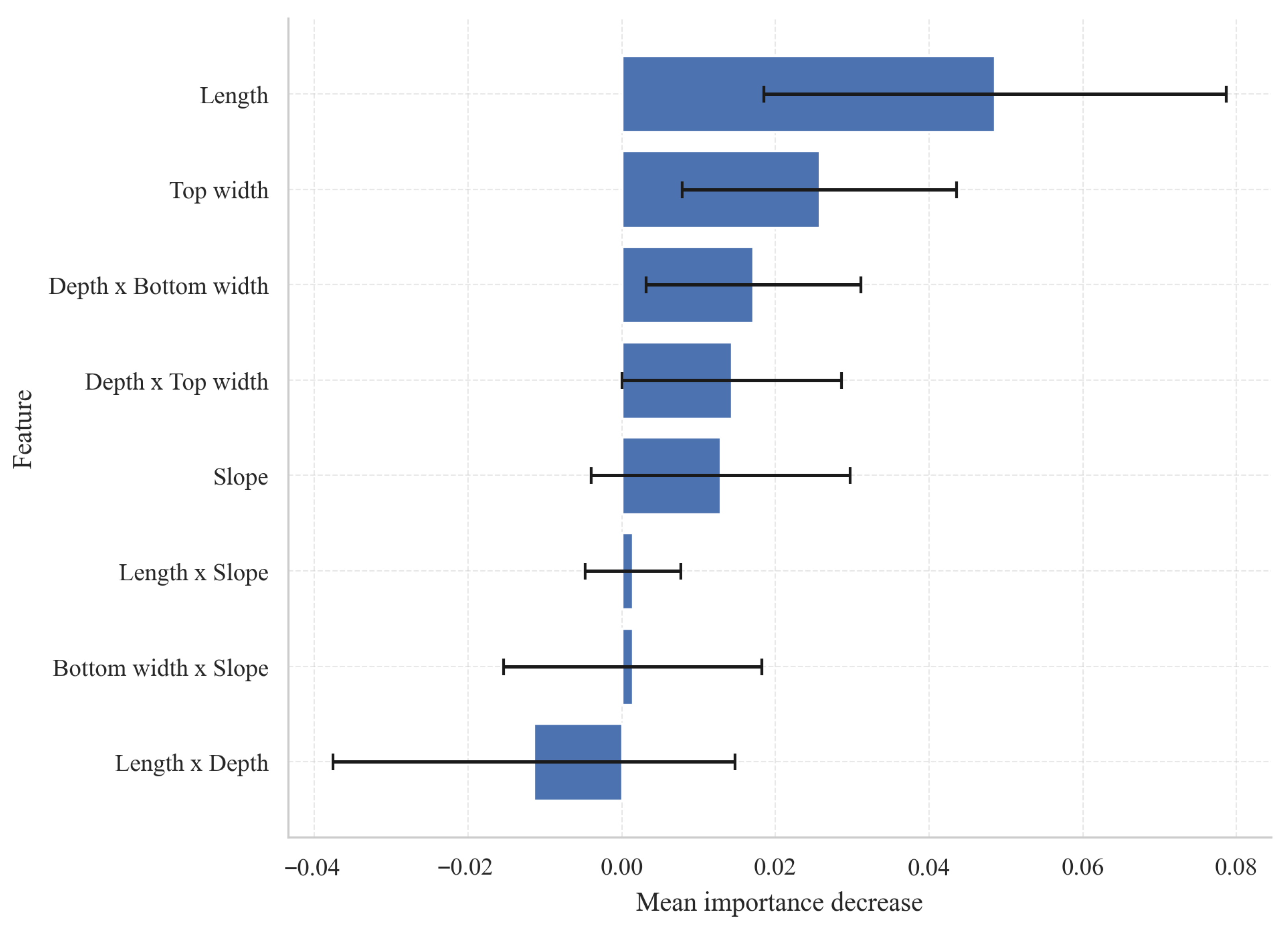
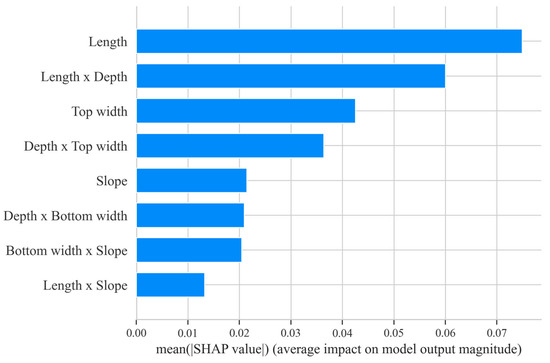
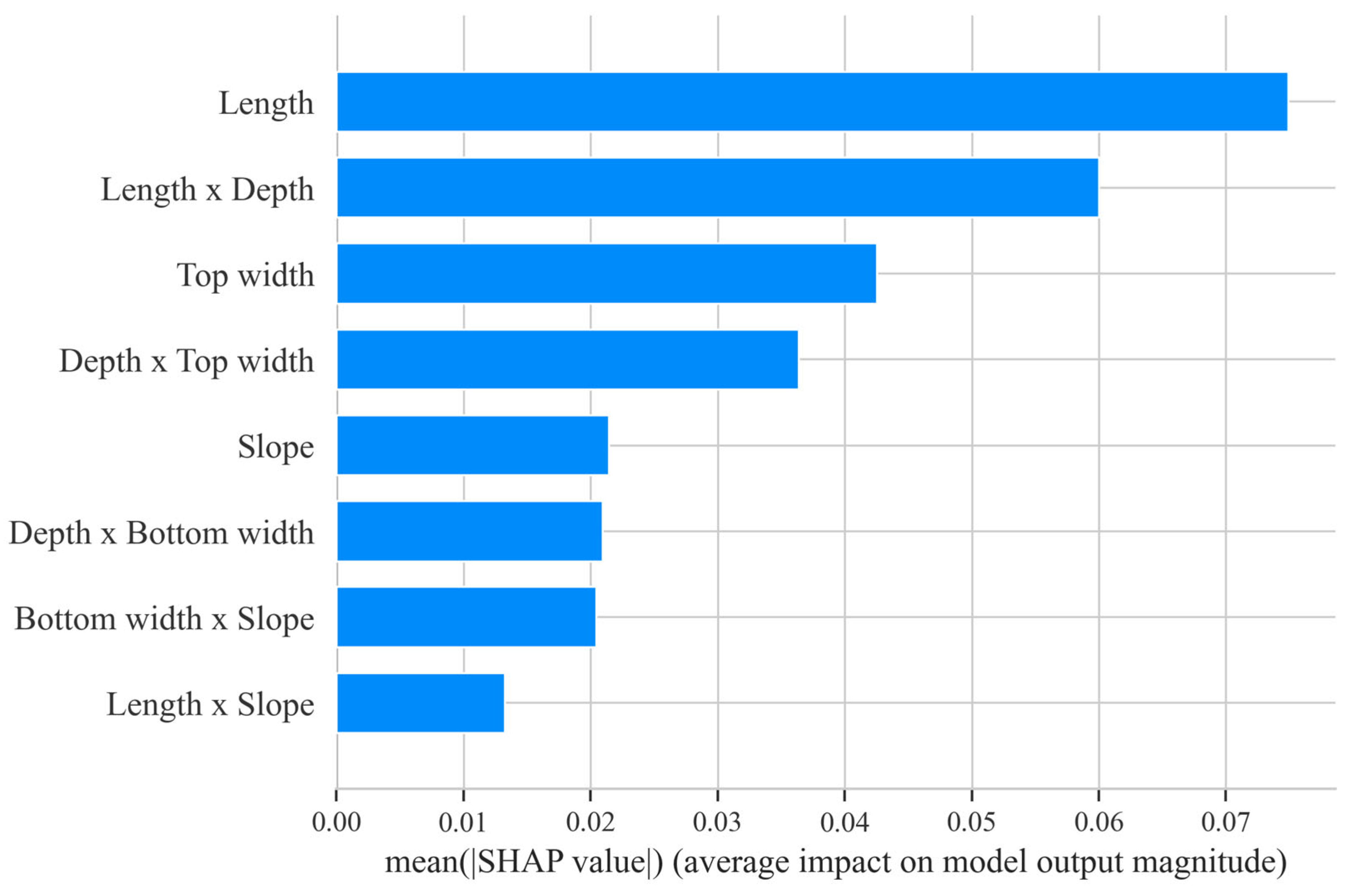
Based on the comprehensive results of various feature importance metrics (Figure 17, Figure 18 and Figure 19), Length, Length × Erosion Gully Depth, Average Top Width, and Erosion Gully Depth × Average Top Width are the core variables influencing model classification. Among these, Length performs exceptionally well across all three metrics—native importance, replacement importance, and Mean |SHAP|—indicating that gully length is a key scale factor for distinguishing erosion gully development levels. Although the replacement importance of Length × Erosion gully depth is negative, its native importance and SHAP values are high, indicating that this variable plays a strong explanatory role in the tree model structure, though its stability is slightly weaker under sample perturbation. Average top width and its interaction term with gully depth also make significant contributions, indicating that lateral widening and its coupling with the downcutting process are crucial for classification results. In contrast, the contributions of Erosion gully depth × Average bottom width, slope, Average bottom width × slope, and Length × slope are relatively low; these are auxiliary variables primarily used to supplement the combined information between slope energy and gully morphology.
Figure 17.
Importance of native features in Random Forest.
Figure 18.
Substitution importance results.
Figure 19.
SHAP global importance bar chart.
4.2. SHAP Global Interpretation
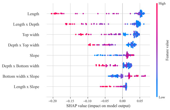
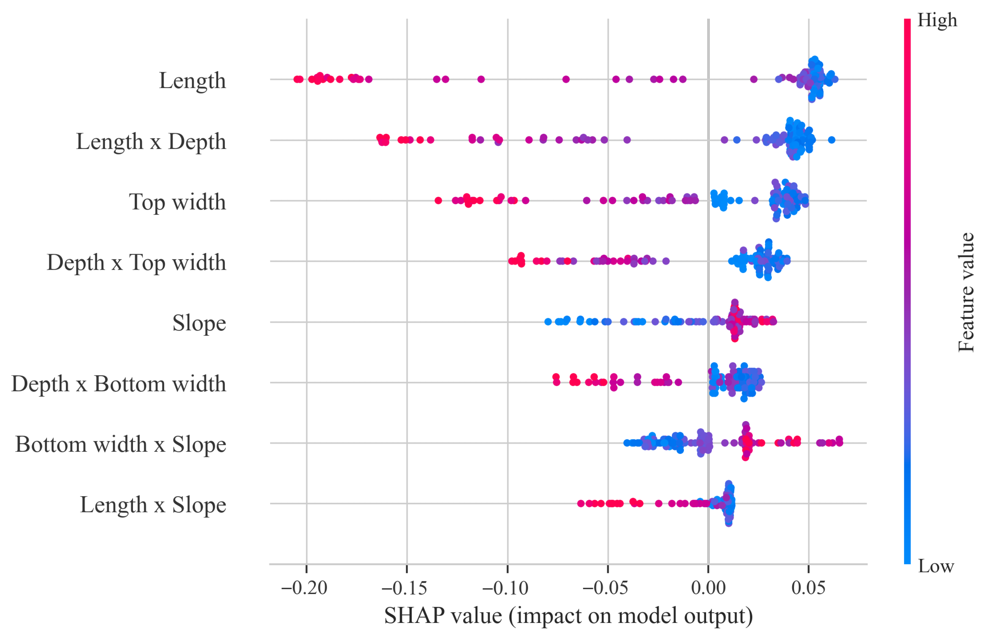
Figure 20 shows the SHAP swarm plot for the Random Forest model, illustrating the direction, strength, and inter-sample variation of each feature’s contribution to the classification results. Overall, Length, Length × Depth, Top width, and Depth × Top width rank highest, indicating that the longitudinal scale of the channel and its coupling with downward incision and lateral widening are the dominant factors influencing classification. The SHAP values on the horizontal axis represent the direction and magnitude of influence on the model’s output; the larger the absolute value, the stronger the feature’s contribution to sample discrimination. The color gradient from blue to red represents feature values ranging from low to high. It can be observed that for variables such as Length, Length × Depth, and Top width, samples with high values are predominantly distributed in the negative SHAP region, while those with low values appear more frequently in the positive region. This indicates that larger scale combinations tend to reduce the output of the current class, whereas smaller values are more likely to shift samples toward a different classification result. In contrast, the distributions for Slope, Bottom width × Slope, and Length × Slope are more concentrated, suggesting that their overall influence is relatively weaker and that they primarily serve a supplementary corrective role.
Figure 20.
SHAP Beeswarm Summary.
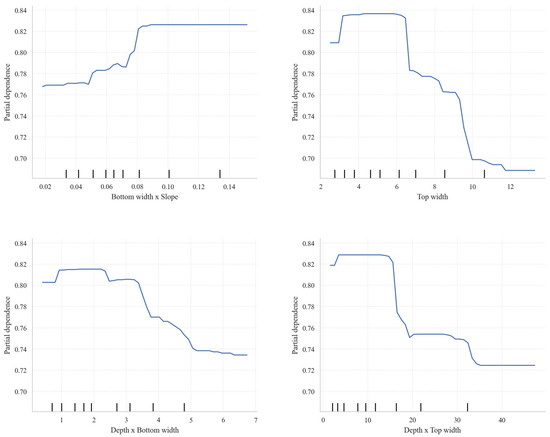
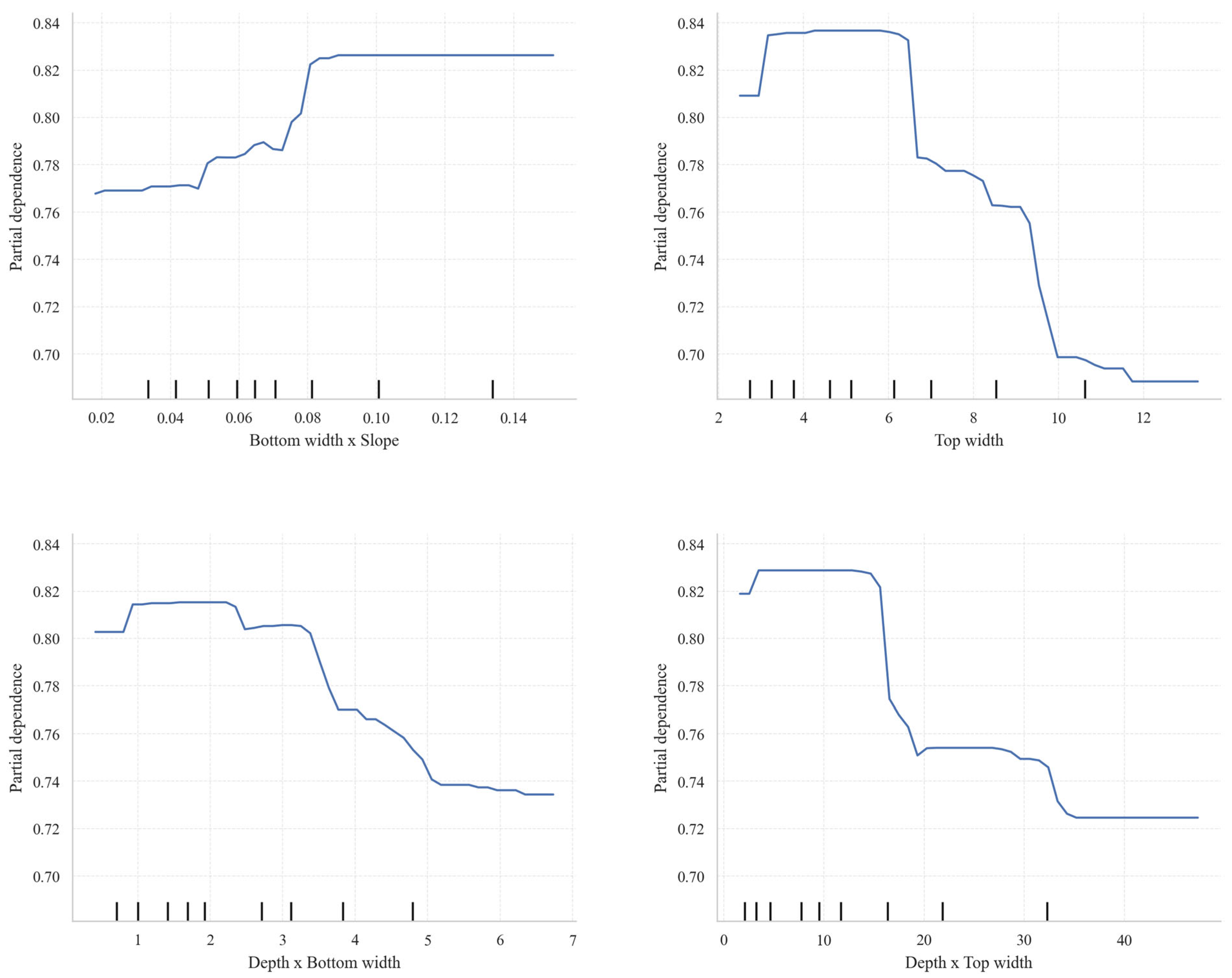
Figure 21 presents the average bias-dependence curves for the four key features, providing a more intuitive illustration of their marginal impact on the model’s output. It can be seen that Bottom width × Slope shows a clear positive correlation with the model output; after the feature value increases from a low level to approximately 0.08, the bias dependence rises from about 0.77 to around 0.83 and tends to stabilize, indicating that the promotional effect of this interaction term on class discrimination gradually saturates once it reaches a certain level. In contrast, Top width, Depth × Bottom width, and Depth × Top width all exhibit negative effects, meaning that as these variables increase, the model output continues to decrease. Among them, Top width shows the most pronounced decrease in the range of approximately 6.5 to 10, while Depth × Top width exhibits a sharp drop around 15 to 20, indicating that the model exhibits a clear threshold response to these features.
Figure 21.
Univariate PDP Plot.
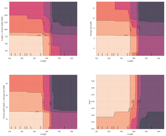
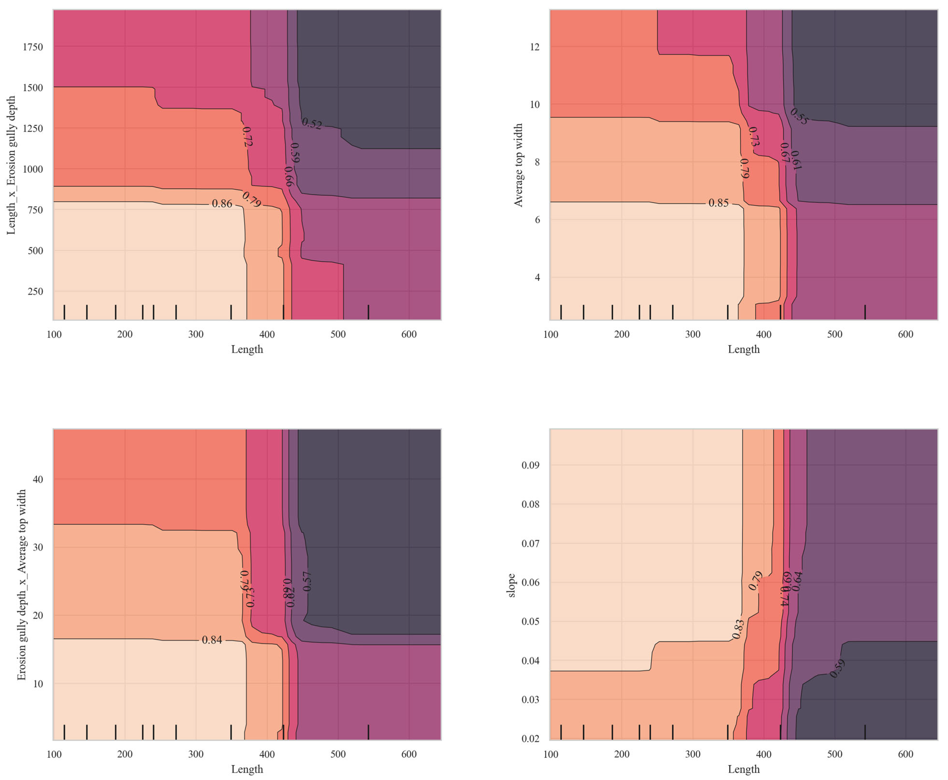
Figure 22 illustrates the two-dimensional partial dependence relationships for four sets of key feature combinations. Overall, all four figures exhibit distinct partitioning structures, indicating that the model’s response to feature combinations exhibits significant nonlinearity and threshold effects. Taking the combination of Length with other variables as an example, when Length is below approximately 380–430, the model output remains generally high; however, once this range is exceeded, the contour lines rapidly contract and the predicted values drop significantly, indicating that gully length is the primary controlling scale influencing classification. At the same time, increases in the combinations of Length × Erosion gully depth, Average top width, and Erosion gully depth × Average top width typically further drive the output downward, suggesting a synergistic inhibitory effect between gully length and gully depth or top width. In contrast, changes in the combination of slope and Length are more concentrated as a step change along the Length direction.
Figure 22.
Two-dimensional partial dependence plot.
4.3. Local Explanatory Analysis
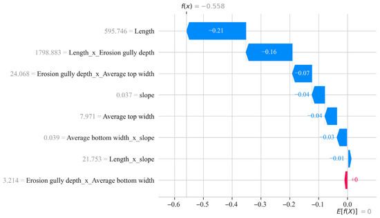
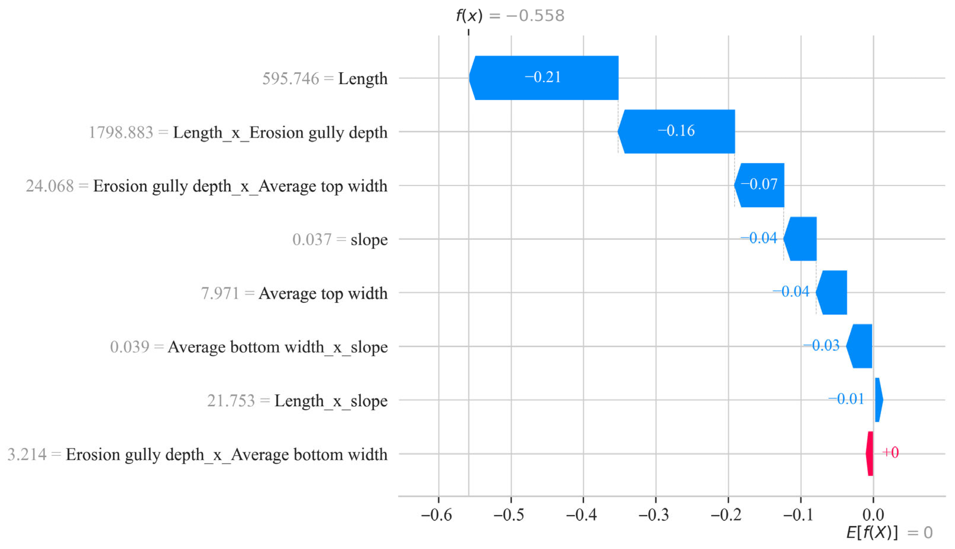
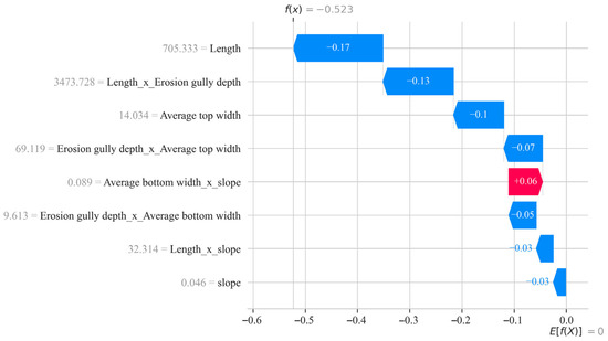
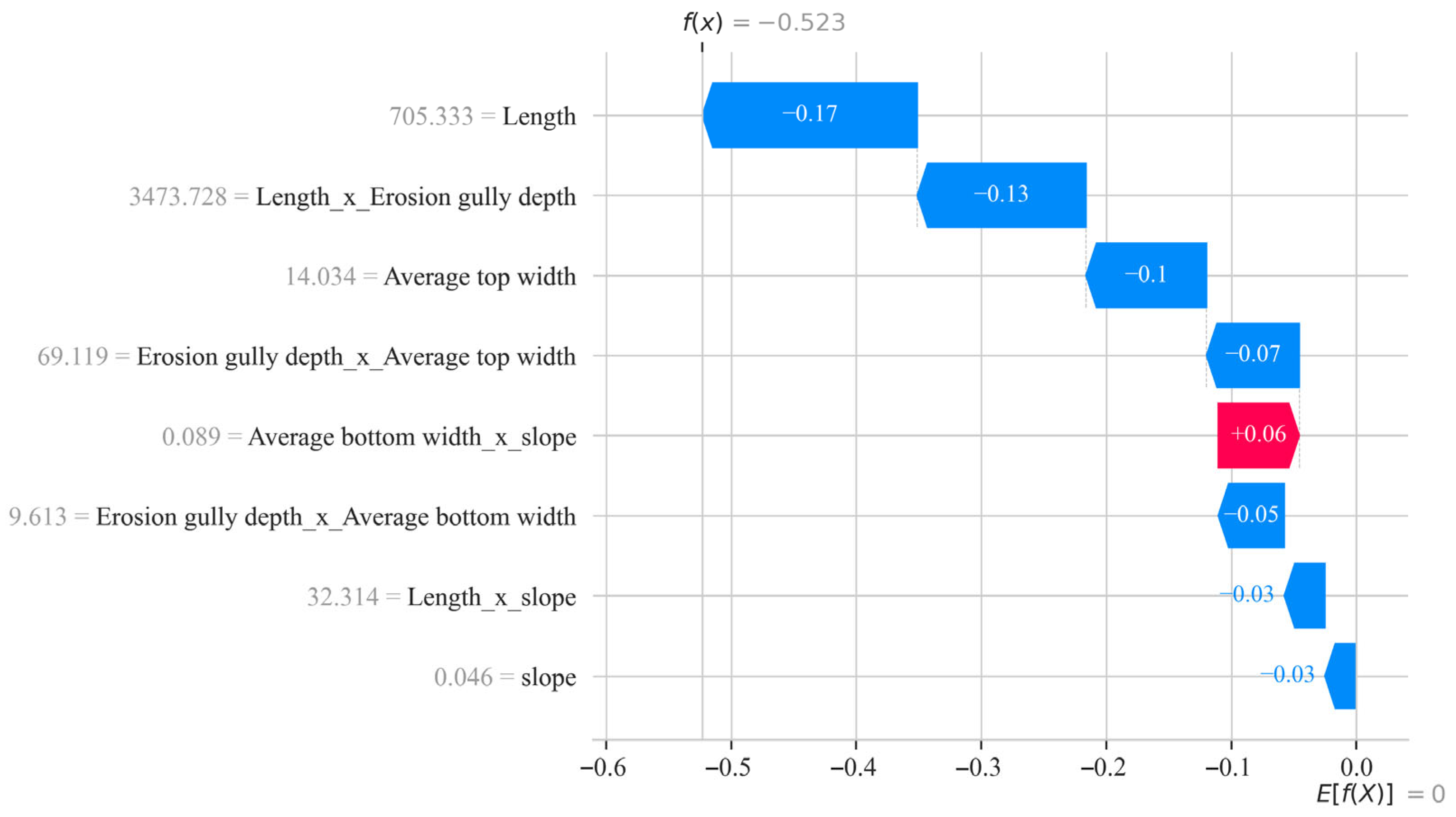
SHAP waterfall plots (Figure 23 and Figure 24) illustrate the local decision-making processes of the Random Forest model for two individual samples, indicating that the model primarily makes classification judgments by “accumulating evidence” from core-scale variables and their interaction terms. Overall, the final output values for the two samples were −0.558 and −0.523, respectively, both indicating that multiple features collectively pushed the prediction results in the same direction. Among these, Length and Length × Erosion Gully Depth were the primary negative drivers in both figures, contributing the most significantly, suggesting that gully length and its coupling with gully depth are the core determinants of the model’s classification; Average top width and Erosion gully depth × Average top width also consistently provide negative contributions, indicating that the lateral widening of the gully and its interaction with the downcutting process are equally important. In contrast, variables such as slope and Length × slope have weaker influences and primarily serve a supplementary corrective role.
Figure 23.
SHAP waterfall explanation for typical sample 1.
Figure 24.
SHAP waterfall explanation for typical sample 2.
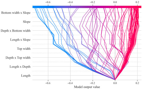
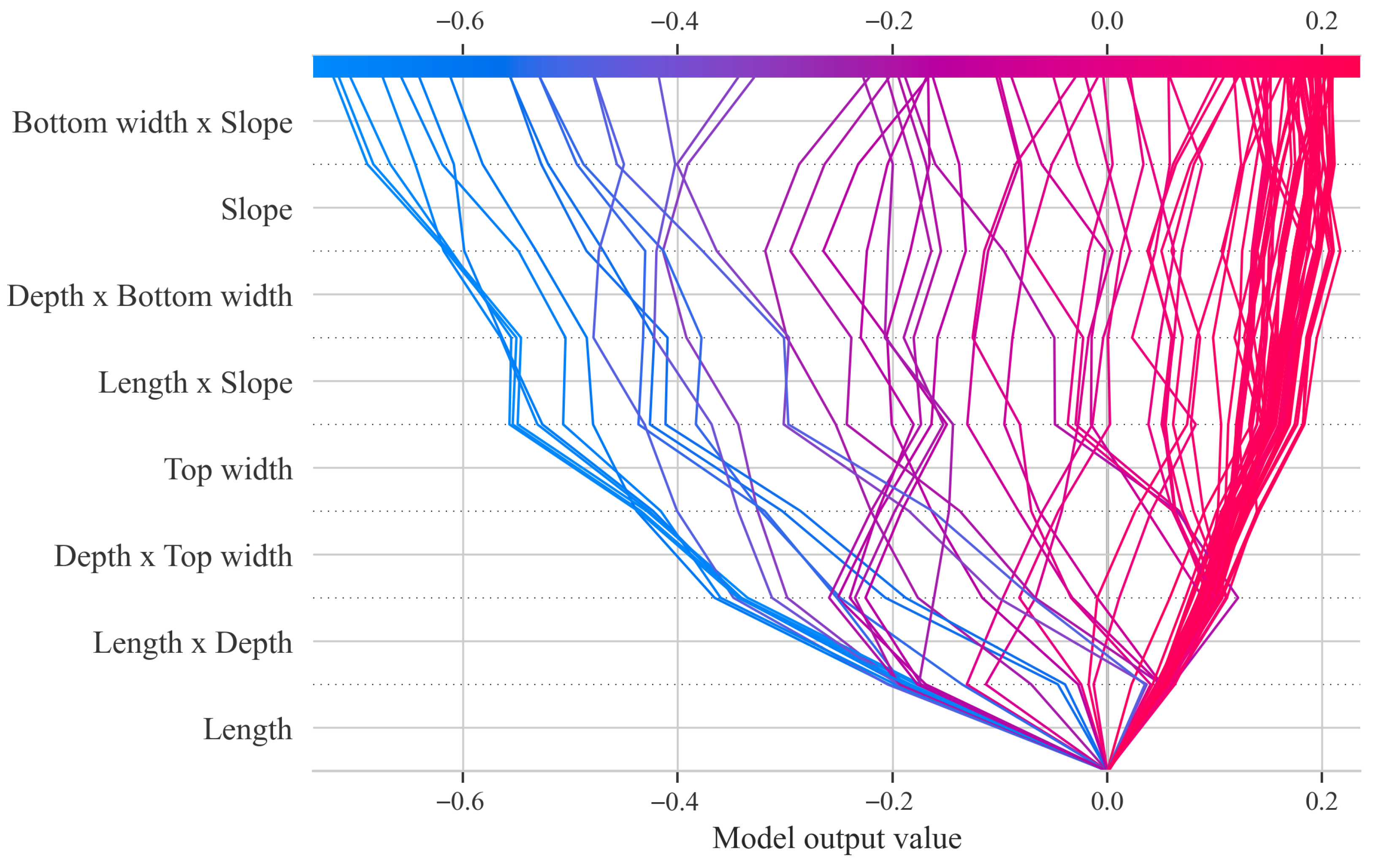
Figure 25 shows the SHAP decision tree for the Random Forest model, illustrating how the prediction path changes across multiple samples as key features are progressively applied. The horizontal axis represents the model output, the vertical axis lists features sorted by importance, and the line segments depict the process by which different samples start from a baseline value, pass through the sequential application of each feature, and ultimately reach the predicted result. Overall, Length and Length × Depth are located at the bottom of the decision path and exert the greatest influence on the majority of samples, indicating that channel length and its interaction with channel depth are the core factors influencing the model’s classification. Subsequently, features such as Depth × Top width, Top width, and Length × Slope continue to adjust the prediction direction, causing the samples to gradually diverge.
Figure 25.
SHAP Decision Path Diagram of the Random Forest Model.
5. Discussion
5.1. Geomorphological Implications of the Controlling Factors for Erosion Gully Grades
The findings of this study suggest that variations in erosion gully classifications cannot be attributed to a single morphological parameter; rather, they represent an integrated outcome of the combined influences of longitudinal extension, vertical deepening, and lateral widening of the gullies. Analyses employing Random Forest feature importance, permutation importance, and SHAP values consistently highlight that gully length, average top width, and their interaction terms with gully depth contribute substantially to classification performance. This implies that gully length and top width serve not only as critical metrics for differentiating between Small and Medium gully types but also partially embody the geomorphological progression of gully evolution from initial incision through subsequent development stages. Notably, the pronounced significance of the interaction terms Length × Erosion Gully Depth and Erosion Gully Depth × Average Top Width underscores a distinct synergistic interplay among gully elongation, vertical incision, and lateral erosion processes. Conversely, slope gradient and certain slope-related variables exhibit a comparatively limited discriminatory capacity within the present dataset, potentially due to the relatively homogeneous distribution of slope gradients across the study area. Consequently, the results are best interpreted as a characterization of the morphological determinants governing erosion gully grading. It is important to acknowledge that, as environmental background factors such as precipitation, soil characteristics, land use, and vegetation cover have not yet been incorporated, the geomorphological interpretations of controlling factors currently rest primarily on morphological statistical associations. Future integrative analyses incorporating these environmental drivers are anticipated to enhance the mechanistic understanding of erosion gully development processes.
5.2. Methodological Advantages and Limitations
The principal methodological advantage of this study resides in the integration of the robust nonlinear classification capabilities of the Random Forest algorithm with the interpretability afforded by SHAP (SHapley Additive exPlanations). This combination facilitates not only the accurate classification of erosion gully grades but also the elucidation of the key variables driving the model’s discriminative performance, including the directionality of their effects. In contrast to opaque “black-box” models that prioritize classification accuracy alone, the proposed framework is particularly well-suited for geomorphological investigations that require a balance between predictive performance and process interpretability. Furthermore, the study systematically assessed model performance through the application of cross-validation, grid search optimization, comparative analyses across multiple modeling approaches, and evaluation of different strategies for addressing class imbalance. The findings demonstrate that, given the current sample conditions, the Random Forest model outperforms logistic regression, support vector machines (SVM), decision trees, and backpropagation neural networks (BPNN) in overall performance. Additionally, the class weighting technique employed exhibits favorable comprehensive results.
Nonetheless, it is important to acknowledge that the methodological framework presented herein remains amenable to further refinement. First, limitations related to field survey conditions and the costs associated with sample collection have resulted in a relatively small sample size with an imbalanced distribution across erosion gully grades. Consequently, the model’s capacity to accurately identify minority classes and its stability across different data partitions warrant further validation using larger and more balanced datasets. Second, although the incorporation of interaction terms enhances the representation of the coupled developmental characteristics of erosion gullies, this approach may inadvertently increase feature collinearity, particularly under conditions of limited sample size. Future research could therefore benefit from the application of advanced feature selection and dimensionality reduction techniques to optimize the variable set. Finally, as the study’s samples are predominantly drawn from a single geographic region, the generalizability of the findings is primarily confined to hierarchical classification within this specific context. Extending the applicability of the results to other black soil regions or diverse topographic settings will require progressive validation through cross-regional data integration and external sample testing.
5.3. Implications for Future Research and Management Practices
The findings of this study suggest that the classification of erosion gullies is anticipated to transition from conventional empirical assessments toward a more analytical framework characterized by “multi-factor coupling and interpretable modeling.” Current investigations reveal that classification approaches relying solely on morphological parameters can achieve a considerable level of accuracy in determining erosion gully grades, while also identifying critical features such as gully length, crest width, and their interactions. This establishes a robust foundation for advancing future research from “morphological classification” to “mechanism interpretation.” Looking ahead, the integration of environmental variables—including rainfall erosive force, soil properties, land use, vegetation cover, and runoff conditions—into existing models, alongside the continuous augmentation of sample data across different grades, particularly medium- and high-grade erosion gullies, is expected to enhance model stability, interpretive depth, and regional applicability. Furthermore, the incorporation of diverse unbalanced learning strategies and cross-regional validation techniques will facilitate a more comprehensive evaluation of the model’s generalizability.
From a practical management perspective, the identification framework developed in this study offers a valuable reference for the rapid surveying and graded management of erosion gullies. By employing technical methodologies such as Real-Time Kinematic (RTK) positioning, unmanned aerial vehicle (UAV) mapping, and remote sensing interpretation, key parameters—including gully length, depth, and crown width—can be efficiently extracted, enabling preliminary classification and risk assessment. This approach holds significant practical implications for monitoring erosion gullies within the Black Soil Region, prioritizing remediation efforts, and optimizing the allocation of inspection resources. Nonetheless, under current research conditions, this method is best utilized as a complementary tool to field surveys and existing classification standards, primarily serving preliminary screening and auxiliary decision-making purposes. With future expansions in sample size, refinement of variable systems, and advancements in external validation, this framework is anticipated to assume a more prominent role in the precise monitoring and management of erosion gullies.
6. Conclusions
- (1)
- The morphological parameters of erosion gullies within the study area serve as effective indicators of gully characteristics across varying developmental stages. Notably, gully length, depth, and average crest width exhibit significant variation among different developmental levels, suggesting that alterations in erosion gully grading are predominantly reflected in scale-related attributes such as longitudinal extension, vertical incision and deepening, as well as lateral expansion. These morphological features offer a robust foundation for the classification and identification of erosion gullies.
- (2)
- Among the five evaluated models—logistic regression, support vector machines, decision trees, backpropagation neural networks, and random forests—the random forest model demonstrated superior overall performance. Specifically, its accuracy on the test set, F1-macro score, and balanced accuracy were 0.9143, 0.8087, and 0.8427, respectively. These results indicate strong classification accuracy, generalizability, and stability, rendering the random forest model particularly suitable for classifying black soil erosion gully grades.
- (3)
- In addressing challenges related to limited sample size and class imbalance, the class weight balancing strategy outperformed both SMOTE-based oversampling and undersampling techniques. This approach effectively enhanced the recognition of minority classes while preserving model stability, thereby suggesting that a random forest model incorporating class weight adjustments is better aligned with the data characteristics of this study.
- (4)
- Analyses of feature importance, permutation importance, and SHAP (SHapley Additive exPlanations) values reveal that gully length, average crest width, and interaction terms such as gully length × gully depth and gully depth × average crest width constitute the principal factors influencing gully grade classification. These findings imply that variations in gully grades are chiefly governed by the synergistic processes of gully elongation, vertical incision, and lateral widening. The integration of the Random Forest model with SHAP interpretation not only achieves high-precision grade classification but also provides an interpretable methodological framework for elucidating erosion gully development mechanisms and facilitating targeted, graded management strategies.
Author Contributions
Conceptualization, M.W.; methodology, M.H., F.W. and F.X.; software, M.H.; validation, M.W. and F.X.; formal analysis, Y.L.; investigation, Y.L. and C.W.; resources, C.W.; data curation, M.H. and F.W.; writing—original draft preparation, M.H. and F.W.; writing—review and editing, M.H., F.W., C.W. and F.X.; visualization, M.W. and Y.L.; supervision, M.W. and F.X.; project administration, M.W. and Y.L.; funding acquisition, M.W. and Y.L. All authors have read and agreed to the published version of the manuscript.
Funding
The authors are grateful for financial support by National Natural Science Foundation of China (42401175); Heilongjiang Provincial Natural Science Foundation of China (LH2023E117); Heilongjiang Provincial Research Institutes Scientific Research Business Fund Project (CZKYF2024-1-A006).
Institutional Review Board Statement
Not applicable.
Informed Consent Statement
Not applicable.
Data Availability Statement
Data will be made available on request.
Acknowledgments
Generative AI and AI-assisted technologies have been utilized exclusively during the writing phase to enhance the manuscript’s readability and linguistic quality. This technology has been employed under human oversight and management, with the authors meticulously reviewing and refining the outcomes prior to the finalization of the paper.
Conflicts of Interest
The authors declare that they have no known competing financial interests or personal relationships that could have appeared to influence the work reported in this paper.
References
- Castillo, C.; Gómez, J.A. A century of gully erosion research: Urgency, complexity and study approaches. Earth-Sci. Rev. 2016, 160, 300–319. [Google Scholar] [CrossRef] [Scilit]
- Vanmaercke, M.; Panagos, P.; Vanwalleghem, T.; Hayas, A.; Foerster, S.; Borrelli, P.; Rossi, M.; Torri, D.; Casali, J.; Borselli, L.; et al. Measuring, modeling, and managing gully erosion at large scales: A state of the art. Earth-Sci. Rev. 2021, 218, 103637. [Google Scholar] [CrossRef] [Scilit]
- Vanmaercke, M.; Poesen, J.; Van Mele, B.; Demuzere, M.; Bruynseels, A.; Golosov, V.; Bezerra, J.F.R.; Bolysov, S.; Dvinskih, A.; Frankl, A.; et al. How fast do gully headcuts retreat? Earth-Sci. Rev. 2016, 154, 336–355. [Google Scholar] [CrossRef] [Scilit]
- Borrelli, P.; Robinson, D.A.; Fleischer, L.R.; Lugato, E.; Ballabio, C.; Alewell, C.; Meusburger, K.; Modugno, S.; Schütt, B.; Ferro, V.; et al. An assessment of the global impact of 21st century land use change on soil erosion. Nat. Commun. 2017, 8, 2013. [Google Scholar] [CrossRef] [Scilit]
- Poesen, J. Soil erosion in the Anthropocene: Research needs. Earth Surf. Process. Landf. 2018, 43, 64–84. [Google Scholar] [CrossRef] [Scilit]
- Keesstra, S.D.; Bouma, J.; Wallinga, J.; Tittonell, P.; Smith, P.; Cerdà, A.; Montanarella, L.; Quinton, J.N.; Pachepsky, Y.; van der Putten, W.H.; et al. Forum paper: The significance of soils and soil science toward the realization of the UN Sustainable Development Goals (SDGs). Soil Discuss. 2016, 2016, 111–128. [Google Scholar]
- Wang, F. Preliminary Study on the Characteristics and Control Concepts of Erosion Gullies in Cold Black Soil Regions; Institute of Engineering Mechanics, China Earthquake Administration: Harbin, China, 2024. [Google Scholar]
- Li, J.; Chen, Y.; Jiao, J.; Chen, Y.; Chen, T.; Zhao, C.; Zhao, W.; Shang, T.; Xu, Q.; Wang, H.; et al. Gully erosion susceptibility maps and influence factor analysis in the Lhasa River Basin on the Tibetan Plateau, based on machine learning algorithms. Catena 2024, 235, 107695. [Google Scholar] [CrossRef] [Scilit]
- Marzolff, I.; Poesen, J. The potential of 3D gully monitoring with GIS using high-resolution aerial photography and a digital photogrammetry system. Geomorphology 2009, 111, 48–60. [Google Scholar] [CrossRef] [Scilit]
- Zhang, X.; Zhang, S.; Meng, X.; Zhang, G.; Zang, D.; Han, Y.; Ai, H.; Liu, H. Remote sensing image segmentation of gully erosion in a typical black soil area in Northeast China based on an improved DeepLabV3+ model. Ecol. Inform. 2024, 84, 102929. [Google Scholar] [CrossRef] [Scilit]
- Zhang, S.; Meng, X.; Zhang, G.; Dai, X.; Yu, Y.; Li, Y.; Zhang, X.; Liu, H. Automated gully erosion extraction in the typical black soil region of Northeast China using a deep learning approach based on multi-source remote sensing data. Catena 2026, 263, 109748. [Google Scholar] [CrossRef] [Scilit]
- Liu, B.; Yuan, Z.; Guo, J.; Wu, S.; Feng, H.; Bu, C.; Siddique, K.H. Extracting gullies using machine learning and deep learning algorithms in the loess hilly and gully region of China. Int. Soil Water Conserv. Res. 2026, 14, 100587. [Google Scholar] [CrossRef] [Scilit]
- Mohebzadeh, H.; Biswas, A.; Rudra, R.; Daggupati, P. Machine learning techniques for gully erosion susceptibility mapping: A review. Geosciences 2022, 12, 429. [Google Scholar] [CrossRef] [Scilit]
- Arabameri, A.; Tiefenbacher, J.P.; Blaschke, T.; Pradhan, B.; Bui, D.T. Morphometric analysis for soil erosion susceptibility mapping using a novel GIS-based ensemble model. Remote Sens. 2020, 12, 874. [Google Scholar] [CrossRef] [Scilit]
- Huang, D.; Su, L.; Zhou, L.; Tian, Y.; Fan, H. Assessment of gully erosion susceptibility using different DEM-derived topographic factors in the black soil region of Northeast China. Int. Soil Water Conserv. Res. 2023, 11, 97–111. [Google Scholar] [CrossRef] [Scilit]
- Mohammady, M.; Davudirad, A. Gully erosion susceptibility assessment using different machine learning algorithms: A case study of the Shazand Watershed in Iran. Environ. Model. Assess. 2024, 29, 249–261. [Google Scholar] [CrossRef] [Scilit]
- Liu, C.; Fan, H.; Wang, Y. Gully erosion susceptibility assessment using three machine learning models in the black soil region of Northeast China. Catena 2024, 245, 108275. [Google Scholar] [CrossRef] [Scilit]
- Zheng, Z.; Yan, T.; Zhao, W.; Qin, W.; Huang, C.; Wang, Y.; Li, Z. Gully erosion susceptibility assessment and SHAP interpretability analysis in sloping farmland of soil-rock dual structure area: A case study of Yimeng Mountain area, China. Geomorphology 2025, 496, 110146. [Google Scholar] [CrossRef] [Scilit]
- Breiman, L. Random forests. Mach. Learn. 2001, 45, 5–32. [Google Scholar] [CrossRef] [Scilit]
- Belgiu, M.; Drăguţ, L. Random forest in remote sensing: A review of applications and future directions. ISPRS J. Photogramm. Remote Sens. 2016, 114, 24–31. [Google Scholar] [CrossRef] [Scilit]
- Biau, G.; Scornet, E. A random forest guided tour. Test 2016, 25, 197–227. [Google Scholar] [CrossRef] [Scilit]
- Maxwell, A.E.; Warner, T.A.; Fang, F. Implementation of machine-learning classification in remote sensing: An applied review. Int. J. Remote Sens. 2018, 39, 2784–2817. [Google Scholar] [CrossRef] [Scilit]
- Li, H.; Jin, J.; Dong, F.; Zhang, J.; Li, L.; Zhang, Y. Gully erosion susceptibility prediction using high-resolution data: Evaluation, comparison, and improvement of multiple machine learning models. Remote Sens. 2024, 16, 4742. [Google Scholar] [CrossRef] [Scilit]
- Fisher, A.; Rudin, C.; Dominici, F. All models are wrong, but many are useful: Learning a variable’s importance by studying an entire class of prediction models simultaneously. J. Mach. Learn. Res. 2019, 20, 1–81. [Google Scholar]
- Nembrini, S.; König, I.R.; Wright, M.N. The revival of the Gini importance? Bioinformatics 2018, 34, 3711–3718. [Google Scholar] [CrossRef] [Scilit] [PubMed]
- Apley, D.W.; Zhu, J. Visualizing the effects of predictor variables in black-box supervised learning models. J. R. Stat. Soc. Ser. B Stat. Methodol. 2020, 82, 1059–1086. [Google Scholar] [CrossRef] [Scilit]
- Lundberg, S.M.; Lee, S.I. A unified approach to interpreting model predictions. In Proceedings of the 31st International Conference on Neural Information Processing Systems, Long Beach, CA, USA, 4–9 December 2017. [Google Scholar]
- Lundberg, S.M.; Erion, G.; Chen, H.; DeGrave, A.; Prutkin, J.M.; Nair, B.; Katz, R.; Himmelfarb, J.; Bansal, N.; Lee, S.-I. From local explanations to global understanding with explainable AI for trees. Nat. Mach. Intell. 2020, 2, 56–67. [Google Scholar] [CrossRef] [Scilit]
- Li, S.; Hai, M.; Zhang, Q.; Zhou, B.; Wang, M.; Zhao, Z. Study on an interpretable prediction model for pile bearing capacity based on SHAP and BP neural networks. Sci. Rep. 2025, 15, 28134. [Google Scholar] [CrossRef] [Scilit] [PubMed]
- Wang, N.; Zhang, H.; Dahal, A.; Cheng, W.; Zhao, M.; Lombardo, L. On the use of explainable AI for susceptibility modeling: Examining the spatial pattern of SHAP values. Geosci. Front. 2024, 15, 101800. [Google Scholar] [CrossRef] [Scilit]
- Yang, R.; Hu, J.; Li, Z.; Mu, J.; Yu, T.; Xia, J.; Li, X.; Dasgupta, A.; Xiong, H. Interpretable machine learning for weather and climate prediction: A review. Atmos. Environ. 2024, 338, 120797. [Google Scholar] [CrossRef] [Scilit]
- Lamane, H.; Mouhir, L.; Moussadek, R.; Baghdad, B.; Kisi, O.; El Bilali, A. Interpreting machine learning models based on SHAP values in predicting suspended sediment concentration. Int. J. Sediment Res. 2025, 40, 91–107. [Google Scholar] [CrossRef] [Scilit]
- Alsumaiei, A.A.; Alrumaidhi, M. Enhancing Soil Water Prediction in Arid Climates Using Multipredictor Machine-Learning Models and SHAP-Based Interpretability. J. Irrig. Drain. Eng. 2026, 152, 04025049. [Google Scholar] [CrossRef] [Scilit]
- Wang, S.; Peng, H. Multiple spatio-temporal scale runoff forecasting and driving mechanism exploration using K-means optimized XGBoost and SHAP. J. Hydrol. 2024, 630, 130650. [Google Scholar] [CrossRef] [Scilit]
- Xi, L.; Qi, Z.; Feng, Y.; Cao, X.; Zou, J.; Han, J. An explainable machine learning approach (SHAP) to assessing desertification risk and its drivers in the Ring-Tarim Basin, 1990–2020. Environ. Impact Assess. Rev. 2026, 118, 108309. [Google Scholar] [CrossRef] [Scilit]
- Mangalathu, S.; Hwang, S.; Jeon, J. Failure mode and effects analysis of RC members based on the machine-learning-based Shapley Additive Explanations (SHAP) approach. Eng. Struct. 2020, 219, 110927. [Google Scholar] [CrossRef] [Scilit]
- Kwak, K.; Lee, E.H. Impact of road transport system on groundwater quality inferred from explainable artificial intelligence (XAI). Sci. Total Environ. 2024, 917, 170388. [Google Scholar] [CrossRef] [Scilit]
- Maurya, R.; Saha, S.; Misra, B.; Chatterjee, D.; Chakraborty, S.; Sarkar, P. Employing Explainable Artificial Intelligence (XAI) for Enhanced Water Quality Assessment. In Proceedings of the 2025 International Conference on Computing, Intelligence, and Application (CIACON), Durgapur, India, 18–19 July 2025; pp. 1–5. [Google Scholar]
- Ma, Q.; Ge, W.; Arab, A.; Butscher, C.; Taherdangkoo, R. Explainable machine learning with ensemble-based uncertainty quantification for groundwater quality indices in the Ganfu Plain, China. Environ. Earth Sci. 2026, 85, 196. [Google Scholar] [CrossRef] [Scilit]
- Yang, S.; Liang, R.; Chen, J.; Wang, Y.; Li, K. Estimating the water quality index based on interpretable machine learning models. Water Sci. Technol. 2024, 89, 1340–1356. [Google Scholar] [CrossRef] [Scilit]
- Choudhary, R.; Kumar, A.; Priyadharsini, C.; Naik, M.M.; Choudhury, M.; Khan, N.A. Predicting water quality index using stacked ensemble regression and SHAP based explainable artificial intelligence. Sci. Rep. 2025, 15, 31139. [Google Scholar] [CrossRef] [Scilit]
- Zhao, Z.; Lei, Y.; Jiang, X.; Leng, Y.; Li, W.; Zhao, W. Explainable machine learning reveals drivers of ecological quality in a karst watershed: Implications for sustainable management of the Mawei river basin, China. Int. J. Digit. Earth 2026, 19, 2600876. [Google Scholar] [CrossRef] [Scilit]
- Aldrees, A.; Khan, M.; Taha, A.T.B.; Ali, M. Evaluation of water quality indexes with novel machine learning and SHapley Additive ExPlanation (SHAP) approaches. J. Water Process Eng. 2024, 58, 104789. [Google Scholar] [CrossRef] [Scilit]

Disclaimer/Publisher’s Note: The statements, opinions and data contained in all publications are solely those of the individual author(s) and contributor(s) and not of MDPI and/or the editor(s). MDPI and/or the editor(s) disclaim responsibility for any injury to people or property resulting from any ideas, methods, instructions or products referred to in the content. |
© 2026 by the authors. Licensee MDPI, Basel, Switzerland. This article is an open access article distributed under the terms and conditions of the Creative Commons Attribution (CC BY) license.