Vision-Guided Dual-Loop Control of a Truck-Mounted Electric Water Cannon for Autonomous Fire Suppression

Abstract

Fire trucks equipped with truck-mounted electric water cannons are key mobile firefighting assets for urban and industrial fire response. However, due to the inherent mechanical inertia of the cannon body, its low-frequency motion response cannot match high-frequency control commands, making the system prone to oscillations and control instability. To address this command–execution frequency mismatch, this paper proposes a decoupled dual closed-loop control architecture for truck-mounted electric water cannons on mobile fire trucks: the fast loop is used for fire-source tracking and rapid localization, while the slow loop is used for water-jet aiming alignment. In the fast loop, a 2-D quadrant positioning rule drives the pan–tilt unit to achieve rapid fire tracking and accurate centering. In the slow loop, Kalman-filter-based state estimation and delay-aligned prediction generate feedforward aiming commands; these commands are fused with error feedback and further processed through command limiting and trajectory optimization, ultimately producing smooth and executable angle references. The visual perception module ran at 58 FPS, satisfying the real-time requirement of the proposed system. In five repeated extinguishment tests under controlled open-site conditions, the proposed method successfully completed all trials and reduced the mean extinguishment time to 13.55 s, compared with 15.83 s for the incremental-PID baseline and 23.76 s for the coupled proportional baseline, while also showing smoother correction and less redundant oscillation.

1. Introduction

Fire disasters continue to cause heavy human and economic losses while exposing firefighters to severe operational hazards. According to the National Fire and Rescue Administration of China, 908,000 fires were reported nationwide in 2024, resulting in 2001 deaths, 2665 injuries, and direct property losses of RMB 7.74 billion [1]. The National Fire Protection Association (NFPA) also reported that 1,389,000 fires occurred in the United States in 2023, causing 3670 civilian deaths, 13,350 civilian injuries, and USD 23.2 billion in direct property damage [2]. Beyond civilian losses, firefighting itself remains a high-risk occupation: the NFPA estimated that 63,175 firefighters were injured in the United States in 2023 [3]. These figures highlight the practical need for firefighting systems that can reduce close-range human exposure and improve operational safety in hazardous environments.

In response, firefighting equipment has gradually evolved from fully manual operation to remote operation and partially automated systems. Kang and Lee developed a tele-operation system for an unmanned fire truck to support real-time firefighting tasks [4]. Jin and Zang proposed a remotely controlled water cannon system with an automatic operating mode [5]. Panwar et al. further reviewed automated firefighting vehicle concepts aimed at reducing direct human exposure to hazardous fire scenes [6]. These studies show a clear shift from manual firefighting equipment toward remotely operated and partially automated suppression systems.

At the engineering level, automatic water cannon technologies have also been explored in different countries and for different deployment scenarios. In China, the automatic tracking and positioning jet fire-extinguishing system has been incorporated into the national standard GB51427-2021 [7], and Xin et al. experimentally evaluated an automatic fire water cannon system for large open spaces [8]. In Japan, an autonomous fire water cannon robot has been developed for hazardous petrochemical fire scenarios [9]. In the United Kingdom, firefighting robots equipped with remotely operated or unmanned water cannons have also been used in industrial fire protection [10]. These examples demonstrate the feasibility of automatic water cannon systems in several deployment scenarios. However, they mainly involve fixed firefighting installations, dedicated robots, or industrial water cannon systems, rather than truck-mounted electric water cannons deployed on mobile fire trucks.

This study focuses on a vision-guided electric water cannon mounted on a mobile fire truck. Because of the large mechanical inertia of the truck-mounted cannon, its actuation bandwidth is insufficient to follow the high-frequency updates generated by visual feedback. Consequently, the closed loop is subject to a pronounced mismatch between perception and actuation timescales, which can induce oscillation, redundant correction, and control instability.

To address this issue, a decoupled dual-loop architecture is developed: the fast loop centers the fire source, while the slow loop regulates the water-jet impact point through delay-aware prediction, feedforward–feedback compensation, and command shaping. Based on this architecture, a vision-guided autonomous water cannon system for fire trucks is developed in this paper. The main contributions are threefold. First, a dedicated dataset is constructed to support joint detection of fire sources and water-jet impact points. Second, a dual-loop control architecture is developed to alleviate the perception–actuation bandwidth mismatch in high-inertia truck-mounted water cannons. Third, the proposed method is validated through modeling, stability analysis, field experiments, and baseline comparisons under the tested conditions. A summary of representative research on automatic firefighting water cannon systems and its relation to the present study is provided in Table 1. For convenience of reference, the principal symbols used throughout the manuscript are summarized in Table 2.

Table 1. Summary of Representative Research on Automatic Firefighting Water Cannon Systems.

Research Line	Representative Work	Technical Focus	Relation to This Study
Remote-controlled or semi-automated vehicle-based systems	Kang and Lee [4]; Jin and Zang [5]; Panwar et al. [6]	Remote firefighting; limited automation	Provides engineering background for vehicle-based firefighting automation
Robot-based or unmanned-platform autonomous systems	Fujita et al. [9]	Autonomous mobility, perception, and fire suppression	Demonstrates the feasibility of autonomous firefighting, but with different platform characteristics
Fixed automatic jet fire-extinguishing systems	Xin et al. [8]	Fixed-site automatic suppression	Shows the engineering value of automatic water cannon systems in structured scenarios
Other platform-level firefighting water-cannon applications	Kent Fire and Rescue Service [10]	Aiming and impact-point control	Provides useful control references for this study
This study	This work	Dual-loop control for truck-mounted water cannons	Focuses on truck-mounted outdoor firefighting with perception–actuation mismatch and delay effects

Table 2. Nomenclature of principal symbols used in the manuscript.

Symbol	Description	Symbol	Description
$W_{img},H_{img}$	Image width and height (px)	($x_0$, $y_0$)	Image center (px)
$B_f$	Fire bounding box	$P_f$ = ($x_f$, $y_f$)	Fire-source centroid (px)
$e_p$ = [$e_x$, $e_y{]}^T$	Pixel offset vector (px)	$e_a$ = [$e_{\varphi }$, $e_{\theta }{]}^T$	Attitude-angle deviation vector
$k_{pa}$	Local Jacobian of the calibrated bearing-angle mapping	$p_x,p_y,f$	physical pixel sizes and focal length
$x_{tol},y_{tol}$	Tolerance half-width and half-height	${\sigma }_x,{\sigma }_y$	Centroid-jitter standard deviations
$T_{sf}{,T}_{ss}$	Fast- and slow-loop sampling periods (s)	$t_k=k{T}_{ss}$	k-th sampling instant
s[k]	Estimated target state $[x,y\dot{,x},\dot{y}{]}^T$	F, H	State-transition and observation matrices
Q, R	Process- and observation-noise covariances	${\sigma }_{vision}$	Vision-noise standard deviation
$T_d$	Total equivalent delay	L	Prediction horizon, ceil (Td/$T_{ss}$)
$T_{sensor}$, $T_{comm},$ $T_{flight}$	Sensing, communication, and jet-flight delays	$D_f$	Nozzle-to-target range
(Δ$x_w$, Δ$y_w$)	Jet-impact pixel offset	(Δθ, Δϕ)	Angle deviations mapped from pixel offset
$C_r$	Empirical range coefficient	${\theta }_{ff},{\varphi }_{ff}$	Feedforward azimuth and elevation
$u_{ff},u_{fb}$	Feedforward and feedback commands	$K_p$	Proportional gain matrix
δ	Dead-zone threshold	$u_{des},u_{cmd}$	Desired and saturated commands
$u_{ref}$(t)	Smoothed reference trajectory	${\omega }_{max},{\alpha }_{max}$	Velocity and acceleration limits
Gm(s), Gm(z)	Fast-loop actuator models	$G_{act}$(s), $G_{act}$(z)	Slow-loop actuator models
R(s), R(z)	Trajectory-shaping models	$K_b$	Ballistic sensitivity gain
$M_s$, $M_t$	Sensitivity and complementary-sensitivity peaks	TP, FP, FN, APi, mAP	Detection metrics
$P_f$[k],$P_w$[k]	Fire centroid and jet-impact point	$e_p$[k]	Image-plane alignment error
${NTV}_e$	Normalized total variation of error	$r_{excess}$	Excess ripple ratio
S	Extinguishment success rate (%)	T	Extinguishment time (s)

2. Framework and Control Architecture of the Proposed Fire-Suppression System

2.1. Overall System Architecture

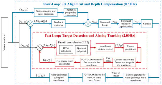
The automatic water cannon fire extinguishing system of the fire truck adopts a dual-loop control structure, including a high-frequency fire source tracking loop and a low-frequency water jet aiming loop. The overall block diagram is shown in Figure 1. The fast loop, serving as the core positioning unit, employs FG-YOLO (FSCNet + GScELAN + YOLOv8) to detect the fire source at a high update rate and outputs its pixel coordinates. The offset between the source centroid and the image center is fed to a pan–tilt controller, which continuously issues rotation commands to keep the target centered in real time. The slow-frequency jet alignment loop operates at a lower update rate and focuses on regulating and correcting the jet impact point. Using as feedback the deviation between the jet-impact pixel coordinates detected by FG-YOLO and the image center, and combining this with Kalman-filter-based fire-source state estimation and motion prediction, it forms a composite feedforward–feedback control strategy. Furthermore, by applying command limiting and trajectory optimization, the loop generates smooth angle commands matched to the water cannon’s mechanical response, thereby achieving precise and stable calibration of the jet impact point.

Figure 1. Water cannon control system block diagram.

The fast-frequency fire source tracking loop and slow-frequency water-jet alignment loop operate independently in a decoupled design: the fast loop handles rapid positioning and continuous fire source tracking, while the slow loop performs precise adjustment of the water-jet landing point. This decoupled design prevents oscillations caused by frequency mismatches between high-frequency visual signals and low-frequency mechanical actuation, thereby ensuring reliable fire detection and suppression in dynamic scenarios.

2.2. Fast Loop: Target Detection and Aiming Tracking

2.2.1. Target Detection Algorithm

The target-recognition module adopts FG-YOLO [11], a lightweight object-detection model optimized for fire and smoke detection. FG-YOLO is based on YOLOv8 and was optimized for real-time fire and smoke detection through efficient feature extraction and multi-scale fusion. In this study, we further adapt FG-YOLO to perform concurrent detection of fire sources and water-jet impact points, enabling the real-time target and impact localization required by the dual-loop control architecture.

To support concurrent detection of fire sources and water-jet impact regions, we built a self-collected dataset, namely the FWS (Fire & Water Stream) dataset. All images were acquired by the authors during controlled combustion and water-discharge experiments using the experimental platform described in Section 4.2.1. The dataset contains scenes in which fire sources and water-jet impact regions appear simultaneously under different backgrounds, illumination conditions, and target positions.

Annotation was performed using LabelImg (App Version:1.8.4) and exported in YOLO format. During training, we applied standard augmentations (e.g., horizontal flips, small rotations, brightness/contrast jitter, and Gaussian noise) and evaluated the model using precision, recall, and mAP metrics. The trained model achieved real-time inference at 58 FPS on an NVIDIA GeForce RTX 4080 (Section 4.1).

2.2.2. Aiming Tracking of Fire Sources

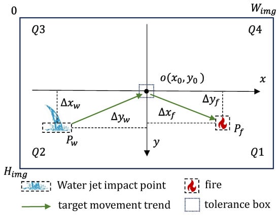
Fire tracking employs a classic image-based control scheme [12]. A two-dimensional cross coordinate system is established with the image center as the origin. Let the captured image resolution be $W_{img}\times H_{img}$. The image center $(x_0,y_0)$ is defined as the reference center, with the $x$-axis positive to the right and the $y$-axis positive downward, where

$$x_0={\displaystyle \frac{W_{img}}{2}},y_0={\displaystyle \frac{H_{img}}{2}}$$

(1)

The x-axis is directed to the right and the y-axis downward. This system divides the image into four quadrants, labeled Q₁ to Q₄ clockwise, with Q₁ located in the bottom-right, as illustrated in Figure 2.

Figure 2. Schematic Diagram of the Cross-Coordinate System.

Within the fast-frequency fire source tracking loop, the FG-YOLO model detects the fire source in each frame and outputs the bounding box coordinates:

$$B_f=\left(x_{min},y_{min},x_{max},y_{max}\right)$$

(2)

The geometric center coordinates of the fire source are calculated as:

$$P_f=\left({\displaystyle \frac{x_{min}+x_{max}}{2}},{\displaystyle \frac{y_{min}+y_{max}}{2}}\right)=(x_f,y_f)$$

(3)

The offset vector (pixel error) is defined as:

$${\mathit{e}}_p=[e_x,e_y{]}^{\top }=[x_f-x_0,y_f-y_0{]}^{\top }$$

(4)

To map the image-plane deviation to the line-of-sight angular deviation, the detected pixel coordinates are first interpreted under the calibrated pinhole camera model [13]. Let $(x,y)$ denote the undistorted image coordinates, and let $(f_x,f_y,c_{x,}{c}_y)$ be the calibrated intrinsic parameters. The corresponding line-of-sight azimuth and elevation relative to the optical axis are

$$\varphi =arctan\left({\displaystyle \frac{x-c_x}{f_x}}\right)$$

(5)

$$\theta =arctan\left({\displaystyle \frac{y-c_y}{f_y}}\right)$$

(6)

For a 3-D point $(X,Y,Z)$, the pinhole projection satisfies $x=f_{x}X/Z+c_x$ and $y=f_{y}Y/Z+c_y$. Hence,

$$\varphi =\mathrm{a}\mathrm{r}\mathrm{c}\mathrm{t}\mathrm{a}\mathrm{n} (X/Z),\theta =\mathrm{a}\mathrm{r}\mathrm{c}\mathrm{t}\mathrm{a}\mathrm{n} (Y/Z)$$

showing that, for line-of-sight centering, the bearing-angle mapping is determined by the image coordinates and calibrated intrinsics and does not require explicit depth recovery. Therefore, the fast loop does not attempt to reconstruct the 3-D fire geometry; it only centers the observed fire-source centroid in the image plane.

Around the image center, the exact mapping in Equations (5) and (6) can be linearized as a constant local Jacobian. This Jacobian is used to obtain the local pixel-to-angle relation in Equation (7) and is written explicitly in Equations (37) and (38) in Section 3.1. This local approximation is appropriate because the fast loop operates in a near-axis centering regime. The camera was calibrated offline before the experiments, providing the intrinsic parameters and a radial distortion model with three coefficients, with a mean reprojection error of 0.3286 pixel. Therefore, the Jacobian used here is derived from calibrated camera parameters rather than from an empirical proportional assumption.

It should also be noted that fire is an extended and time-varying 3-D target. In such a case, depth variation mainly affects the apparent size, contour, and centroid stability of the observed flame region, rather than the first-order mapping from image offset to line-of-sight angle. In this study, these effects are treated as visual measurement disturbances and are mitigated by low-pass filtering, the tolerance box, and the downstream jet-impact feedback loop.

After mapping the pixel error to the line-of-sight (LOS) angular error, the fast loop generates pan–tilt commands using a filtered proportional law with additional low-frequency lag shaping:

$${\mathrm{e}}_{\theta }\left(k\right)=\mathrm{J}\hspace{0.17em}{\mathrm{e}}_p\left(k\right)$$

(7)

$${\mathrm{e}}_{\theta ,f}\left(k\right)=\mathcal{F}\left\{{\mathrm{e}}_{\theta }\right(k\left)\right\}$$

(8)

To suppress frame-to-frame jitter, the LOS angular error is first filtered by a digital low-pass operator $\mathcal{F}\{\cdot \}$ [14,15]. To further improve low-frequency disturbance rejection and stiffness of the fast loop, the filtered signal $e_{\theta ,f}\left(k\right)$ is shaped by a discrete lag compensator $C_{\mathrm{l}\mathrm{a}\mathrm{g}}\left(z\right)$. Denoting the lag-filtered signal as $e_{\theta ,\mathrm{l}\mathrm{a}\mathrm{g}}\left(k\right)$, the lag network is implemented as:

$$e_{\theta ,\mathrm{l}\mathrm{a}\mathrm{g}}\left(k\right)=\beta \hspace{0.17em}{e}_{\theta ,\mathrm{l}\mathrm{a}\mathrm{g}}(k-1)+e_{\theta ,f}\left(k\right)-\alpha \hspace{0.17em}{e}_{\theta ,f}(k-1)$$

(9)

and the incremental command is generated by

$$\Delta {\theta }^{\ast }\left(k\right)=-K_p\hspace{0.17em}{e}_{\theta ,\mathrm{l}\mathrm{a}\mathrm{g}}\left(k\right)$$

(10)

where $e_p\left(k\right)$ is the pixel offset (vector), $J$ is the local Jacobian of the calibrated bearing-angle mapping, and $\mathcal{F}\{\cdot \}$ is implemented as the first-order IIR filter given in Equations (39) and (40). $K_p$ denotes the proportional gain (a diagonal matrix for the two-axis implementation).

In practical implementation, the pan–tilt unit receives command updates at discrete sampling instants and is subject to actuator constraints. Therefore, the computed increment $\Delta {\theta }^{\ast }\left(k\right)$ is processed through (i) saturation/limiting, (ii) rate constraints, and (iii) quantization to the minimum executable step, yielding the final command:

$$\Delta \theta \left(k\right)=\mathcal{Q}\left(\mathrm{s}\mathrm{a}\mathrm{t}\right(\Delta {\theta }^{\ast }\left(k\right),\Delta {\theta }_{\mathrm{m}\mathrm{a}\mathrm{x}}\left)\right)$$

(11)

where $\mathrm{s}\mathrm{a}\mathrm{t}(\cdot )$ limits the increment magnitude (equivalently enforcing the maximum safe angular velocity bound), and $\mathcal{Q}(\cdot )$ denotes quantization to the nearest multiple of the actuator’s minimum angular step.

For clarity, the quadrant-positioning rule used in the on-board implementation is an equivalent sign-only representation of the above proportional law: the quadrant determines the sign (direction) of each axis command, while the command magnitude is determined by the proportional term after filtering and limiting. The sign function is defined as:

$$\mathrm{s}\mathrm{g}\mathrm{n}(x)=\left\{\begin{array}{cc}+1,& x>0,\\ 0,& x=0,\\ -1,& x<0.\end{array}\right.$$

(12)

Accordingly, the quadrant rule is applied to select $\mathrm{s}\mathrm{g}\mathrm{n}\left(e_x\right)$ and $\mathrm{s}\mathrm{g}\mathrm{n}\left(e_y\right)$ (direction), whereas $\mid \Delta \theta \left(k\right)\mid$ is given by the proportional control magnitude.

To suppress jitter caused by detection noise, a tolerance box is defined around the image center, as shown in Figure 2. Let its half-width and half-height be $x_{\mathrm{t}\mathrm{o}\mathrm{l}}$ and $y_{\mathrm{t}\mathrm{o}\mathrm{l}}$, respectively.

These parameters are selected according to two requirements. First, the tolerance region should cover the measurement jitter, namely $x_{\mathrm{t}\mathrm{o}\mathrm{l}}\ge 3{\sigma }_x,y_{\mathrm{t}\mathrm{o}\mathrm{l}}\ge 3{\sigma }_y,$ where ${\sigma }_x$ and ${\sigma }_y$ are estimated from repeated fixed-target image measurements under the calibrated camera setup. Second, the tolerance region should not be excessively large, so that the fire source remains sufficiently close to the image center and the guidance accuracy required by the subsequent slow-loop correction is preserved.

In this study, $x_{\mathrm{t}\mathrm{o}\mathrm{l}}=60$ px and $y_{\mathrm{t}\mathrm{o}\mathrm{l}}=45$ px were adopted. These values exceed the measured centroid-jitter bounds in both directions while remaining small enough to avoid an overly loose centered state. When $\mid e_x\mid \le x_{\mathrm{t}\mathrm{o}\mathrm{l}}$ and $\mid e_y\mid \le y_{\mathrm{t}\mathrm{o}\mathrm{l}}$, the fire-source centroid is regarded as centered and the gimbal command is held. Detection continues in this aligned state without further fine adjustment until the target drifts outside the tolerance region, at which point command updates resume.

The fast-loop parameters were selected from the discrete small-signal model by balancing centering speed, low-frequency stiffness, and the bandwidth limitation imposed by the pan–tilt dynamics, sampling, and delay. The final parameter set was retained only when the closed-loop robustness and sensitivity requirements in Section 3.2.1 were satisfied. Under this implementation, the quadrant rule acts only as a directional selector outside the tolerance region rather than as a pure bang–bang switching law, thereby reducing repeated sign reversals near zero error and suppressing oscillatory behavior in the fast loop.

2.3. Slow Loop: Stabilization Control and Jet Calibration

To effectively address the dynamic mismatch between the high frequency of visual perception and the low frequency of the water cannon mechanical system, and to compensate for inherent system delays in sensing, communication, and water ballistic flight, this section proposes a slow-loop closed-loop structure with delay-aware modeling for controller design and robustness assessment. This method achieves fast, smooth, and precise control of the water cannon aiming process through target state estimation, delay prediction, command limiting, and trajectory processing [16,17,18]. The system control period is $T_{ss}$, and the following process is executed at discrete sampling instants $t_k=k{T}_{ss}$.

• State Estimation and Target Prediction

First, the observation data from the visual sensor are filtered by a Kalman filter. A Kalman filter [19] is used to obtain the smoothed estimated target state $\widehat{s}[k]$ at time k. This state includes the target’s position $(x,y)$ and velocity $(\dot{x},\dot{y})$ in the image coordinate system:

$$\widehat{s}[k]={[\widehat{x}[k],\widehat{y}[k],\widehat{\dot{x}}[k],\widehat{\dot{y}}[k]]}^T$$

(13)

where $(\widehat{x},\widehat{y})$ is the estimated position of the fire source in the image coordinate system (unit: pixels), and $(\widehat{\dot{x}},\widehat{\dot{y}})$ is its estimated velocity (unit: pixels/second).

The Kalman filter is based on a discrete constant velocity model [20]. Its state transition matrix $F$ and observation matrix $H$ are defined as:

$$s_{k+1}=F{s}_k+w_k$$

(14)

$$z_k=H{s}_k+v_k$$

(15)

$$F=[\begin{array}{cccc}1& 0& T_{ss}& 0\\ 0& 1& 0& T_{ss}\\ 0& 0& 1& 0\\ 0& 0& 0& 1\end{array}]$$

(16)

$$H=[\begin{array}{cccc}1& 0& 0& 0\\ 0& 1& 0& 0\end{array}]$$

(17)

The process noise covariance matrix $Q$ and observation noise covariance matrix $R$ are designed as follows:

$$Q=q[\begin{array}{cccc}{T}_{ss}^4/4& 0& T_{ss}^3/2& 0\\ 0& T_{ss}^4/4& 0& T_{ss}^3/2\\ T_{ss}^3/2& 0& T_{ss}^2& 0\\ 0& T_{ss}^3/2& 0& T_{ss}^2\end{array}]$$

(18)

$$R=\mathrm{diag}({\sigma }_{\mathrm{vision}}^2,{\sigma }_{\mathrm{vision}}^2)$$

(19)

Here, the process noise intensity $q={\sigma }_a^2$, and ${\sigma }_{\mathrm{vision}}$ is the standard deviation of the visual observation noise.

The state estimation error covariance matrix $P$ is initialized to a large diagonal matrix:

$$P_0=\mathrm{diag}(100{\mathrm{px}}^2,100{\mathrm{px}}^2,10(\mathrm{px}/\mathrm{s}{)}^2,10\left(\mathrm{px}/\mathrm{s}{)}^2\right)$$

(20)

Based on the current estimated state, a delay-aligned prediction is performed to obtain the image pixel coordinates $\widehat{s}[k+L]$ at the future time $t_k+T_d$. The total delay $T_d=T_{\mathrm{sensor}}+T_{\mathrm{comm}}+T_{\mathrm{flight}}$ includes sensing processing delay, communication and execution delay, and the crucial water projectile flight time. $L=\lceil T_d/T_{ss}\rceil$ is the corresponding prediction step length. Using the constant velocity motion model, the predicted values are:

$$\widehat{x}[k+L]=\widehat{x}[k]+\widehat{\dot{x}}[k]\cdot (L{T}_{ss})$$

(21)

$$\widehat{y}[k+L]=\widehat{y}[k]+\widehat{\dot{y}}[k]\cdot (L{T}_{ss})$$

(22)

The water projectile flight time $T_{\mathrm{flight}}$ is obtained by looking up a value in a table [21,22] based on the range $D_f\left[k\right]$. This table is pre-calibrated from experimental data to compensate for the effects of water flow velocity, launch angle, and air resistance.

The slow-loop controller is organized into (i) a core composite law consisting of a feedforward term from the ballistic inverse solution and a proportional feedback correction in the angle domain, and (ii) command-shaping modules (dead zone, saturation/rate limiting, and trajectory smoothing) that enforce actuator and safety constraints. In Section 3, the frequency-domain analysis is conducted for the core small-signal linear feedback path with an equivalent integer delay, while the effects of the shaping nonlinearities are assessed through time-domain verification.

2.

Feedforward–Feedback Composite Control Law

To unify the dimensions of visual observations and actuator control signals, the pixel deviation in the image plane must be mapped to the water cannon’s attitude angle deviation. Based on the camera’s pinhole model, this mapping is determined by the camera’s intrinsic parameters [13]. The angle deviation $(\Delta \theta ,\Delta \varphi )$ corresponding to the pixel offset $(\Delta x_w,\Delta y_w)$ of the water-jet impact point is calculated as follows:

$$\Delta \theta =\mathrm{a}\mathrm{r}\mathrm{c}\mathrm{t}\mathrm{a}\mathrm{n}({\displaystyle \frac{\Delta x_w\cdot p_x}{f}})$$

(23)

$$\Delta \varphi =\mathrm{a}\mathrm{r}\mathrm{c}\mathrm{t}\mathrm{a}\mathrm{n}({\displaystyle \frac{\Delta y_w\cdot p_y}{f}})$$

(24)

where $p_x,p_y$ are the physical pixel sizes, and $f$ is the camera focal length. In implementation we use the exact arctangent mapping Equations (23) and (24), while the frequency-domain model linearizes it around the operating point, yielding the constant Jacobian used in Equation (49).

The control command is composed of feedforward and feedback terms:

Feedforward term calculation: Based on the delay-aligned predicted future target state ŝ [$k+L$] and the latest available target range $D_f$[k]. The feedforward term is used to generate the initial aiming angles of the water cannon. The feedforward azimuth angle ${\theta }_{ff}\left[k\right]$ is determined from the horizontal bearing of the predicted future target centroid obtained from ŝ[k+L], while the feedforward elevation angle is obtained from the empirical inverse mapping of the horizontal distance $D_f$ from the nozzle to the target. Under the tested operating conditions, the range variation within one slow-loop interval is small; therefore, the latest measured $D_f$[k] is used as the delay-aligned range approximation for feedforward pre-aiming. Under a fixed spray operating condition on the same experimental platform, the following empirical range relation is adopted:

$$D_f=C_r\mathrm{s}\mathrm{i}\mathrm{n}\left(2\varphi \right)$$

(25)

where $C_r$ is the empirical range coefficient. This relation is used for feedforward pre-aiming under fixed operating conditions [23]. Its form is inspired by the basic functional relationship between range and launch angle in ideal projectile motion, and is used to provide an overall approximation of the effective range of the real water jet rather than a high-fidelity fluid-dynamics model. Accordingly, its inverse mapping can be explicitly written as:

$${\varphi }_{ff}=f_r^{-1}(D_f)={\displaystyle \frac{1}{2}}\mathrm{a}\mathrm{r}\mathrm{c}\mathrm{s}\mathrm{i}\mathrm{n}\left({\displaystyle \frac{D_f}{C_r}}\right)$$

(26)

where ${\varphi }_{ff}$ is the feedforward elevation angle. Since the empirical relation $D_f=C_r\mathrm{s}\mathrm{i}\mathrm{n}\left(2\varphi \right)$ yields a two-valued inverse solution for $\varphi \in (0,\pi /2)$, the low-elevation operating branch ${\varphi }_{ff}\in (0,\pi /4)$ is selected to ensure a unique definition of the feedforward elevation angle and consistency with the actual operating elevation range of the experimental platform. Under this condition, the inverse mapping is valid for $0\le D_f\le C_r$.

The empirical range coefficient $C_r$ is identified offline through a static range calibration experiment. Under fixed pump pressure, nozzle opening, and installation conditions, several representative elevation angles ${\varphi }_i$ are selected, and the corresponding horizontal impact distances $D_i$ of the steady jet are measured. The coefficient $C_r$ is then identified using the least-squares criterion:

$${\widehat{C}}_r=\mathrm{a}\mathrm{r}\mathrm{g} \underset{C_r}{\mathrm{m}\mathrm{i}\mathrm{n}}\sum _{i=1}^N{\left(D_i-C_r\mathrm{s}\mathrm{i}\mathrm{n}\left(2{\varphi }_i\right)\right)}^2$$

(27)

Its closed-form solution is:

$${\widehat{C}}_r={\displaystyle \frac{\sum _{i=1}^N{D}_i\mathrm{s}\mathrm{i}\mathrm{n}\left(2{\varphi }_i\right)}{\sum _{i=1}^N{\mathrm{s}\mathrm{i}\mathrm{n}}^2\left(2{\varphi }_i\right)}}$$

(28)

Therefore, the feedforward control input can be expressed as:

$$u_{ff}[k]=({\theta }_{ff}[k],{\varphi }_{ff}[k])$$

(29)

where ${\theta }_{ff}[k]$ is generated from the delay-aligned predicted future target state ŝ[k+L], and ${\varphi }_{ff}[k]$ is generated from the empirical inverse mapping in Equation (26). This empirical inverse mapping is used only to generate the initial elevation command of the slow loop under fixed operating conditions, and the residual modeling error is further compensated by the subsequent closed-loop correction based on jet-impact feedback.

Feedback Term Calculation: Simultaneously, based on the pixel offset $\Delta \left[k\right]=(\Delta \mathrm{x}[k],\Delta y[k]{)}^T$ between the current water-jet impact point coordinates $\left(x_w\right[k],y_w[k\left]\right)$ and the image center $(x_0,y_0)$, a proportional correction is calculated:

$$u_{fb}\left[k\right]=K_p\hspace{0.17em}\Delta \left[k\right]$$

(30)

where $K_p$ is the proportional gain matrix. The slow-loop gains were tuned in two stages [15]. An initial gain range was obtained from the approximate small-signal model by considering the desired convergence rate together with the bandwidth limitation caused by actuator inertia and loop delay. The provisional gains were then refined under the implemented actuator constraints, including dead zone, saturation, rate limiting, and command shaping. The final gains were accepted only when the resulting closed loop satisfied the prescribed robustness and sensitivity requirements.

To suppress minor jitter caused by sensor noise, a dead zone mechanism is introduced:

$$u_{fb}[k]=\{\begin{array}{cc}{K}_p\cdot \Delta \left[k\right]& \mathrm{if}\parallel \Delta \left[k\right]{\parallel }_2 > \delta \\ 0& \mathrm{if}\parallel \Delta \left[k\right]{\parallel }_2 \le \delta \end{array}$$

(31)

The dead-zone threshold is defined as $\delta =3{\sigma }_{\mathrm{v}\mathrm{i}\mathrm{s}\mathrm{i}\mathrm{o}\mathrm{n}}$, where ${\sigma }_{\mathrm{v}\mathrm{i}\mathrm{s}\mathrm{i}\mathrm{o}\mathrm{n}}$ is the standard deviation of the visual measurement noise.

Combination and Limiting: The feedforward and feedback outputs are summed to obtain the desired control command:

$$u_{\mathrm{des}}\left[k\right]=u_{ff}\left[k\right]+u_{fb}\left[k\right]$$

(32)

considering the physical limits of the water cannon actuator, the command undergoes saturation limiting to ensure the angle change per cycle does not exceed the maximum safe angular velocity ${\omega }_{\max }$ constraint:

$$\Delta u_{\max }={\omega }_{\max }{T}_{ss}$$

(33)

$$u_{\mathrm{cmd}}\left[k\right]=\mathrm{sat}\left(u_{\mathrm{des}}\right[k],u_{\mathrm{current}}\pm \Delta u_{\max })$$

(34)

here $u_{\mathrm{current}}$ is the water cannon’s current angle.

3.

Command Trajectory Smoothing

To avoid mechanical shock or overshoot caused by step-like angle commands, a trapezoidal velocity profile algorithm is used for trajectory smoothing [24]. This module takes $u_{\mathrm{cmd}}\left[k\right]$ as the target point and, based on the actuator’s maximum angular velocity ${\omega }_{\max }$ and maximum angular acceleration ${\alpha }_{\max }$ constraints, generates a smooth reference angle trajectory $u_{\mathrm{ref}}\left(t\right)$ over the interval $[t_k,t_{k+1}]$, satisfying the constraints:

$$\mid {\omega }_{\mathrm{ref}}\left(t\right)\mid \le {\omega }_{\max }$$

(35)

$$\mid {\alpha }_{\mathrm{ref}}\left(t\right)\mid \le {\alpha }_{\max }$$

(36)

Through this planner, the discrete command $u_{\mathrm{cmd}}\left[k\right]$ is converted into a continuous-time reference trajectory $u_{\mathrm{ref}}\left(t\right)$, ensuring the stability and convergence of the water cannon system.

For clarity, the principal implementation-related parameters used in the proposed fast and slow loops and their determination bases are summarized in Table 3.

Table 3. Determination Basis of Principal Control Parameters.

Parameter Group	Functional Role	Determination Basis
Calibrated bearing-angle mapping	Converts image-plane deviations into line-of-sight or attitude-angle deviations	Obtained from offline camera calibration.
Fast-loop tolerance bounds ${\epsilon }_u,{\epsilon }_v$	Define the centered region and suppress repeated switching near the image center	Chosen based on repeated fixed-target image measurements and the accuracy requirement of the slow loop.
Fast-loop controller parameters ($K_p$ low-pass filter, lag compensator$)$	Determine centering speed, low-frequency stiffness, and disturbance rejection in the fast loop	Selected from the discrete small-signal model and finalized through robustness and sensitivity screening.
Kalman filter and delay-aligned prediction parameters ($Q,R,P_0,t_f,t_f$)	Provide state estimation and prediction for the slow loop under delay	Set using the discrete constant-velocity model, visual-noise statistics, a pre-calibrated flight-time lookup table, and an equivalent total delay.
Empirical range coefficient $C_r$	Generates the feedforward elevation command for initial aiming	Identified from static range-calibration experiments using least-squares fitting.
Slow-loop feedback and actuator-constraint parameters ($K_b,\delta ,{\omega }_{\mathrm{m}\mathrm{a}\mathrm{x}},a_{\mathrm{m}\mathrm{a}\mathrm{x},}{\tau }_a$)	Realize impact-point correction under executable actuator limits	Determined from the approximate small-signal model, visual-noise statistics, and implemented actuator constraints.

3. Frequency Domain Analysis and Robustness Assessment

3.1. System Modeling and Transfer Function Derivation

(A)

Fast Loop Model

The control process of the fast loop starts from the pixel deviation between the image center and the detected fire-source centroid. As clarified in Section 2.2.2, the fast loop regulates the bearing direction of the detected centroid rather than reconstructing the full 3-D fire geometry. Under the calibrated pinhole camera model, the line-of-sight angular deviation is determined by the undistorted image coordinates and the camera intrinsics. Around the image center, this mapping is linearized as a constant local Jacobian, yielding:

$${\theta }_e\left[k\right]=k_{pa}e\left[k\right]$$

(37)

$$k_{pa}\triangleq {\displaystyle \frac{p}{f}}$$

(38)

where the Jacobian is obtained from the calibrated intrinsic parameters. Therefore, the relation used in the fast-loop model is the local Jacobian of the calibrated bearing-angle mapping around the optical axis, rather than an empirical pixel-to-angle proportional coefficient.

To enhance the system’s disturbance rejection capability, the angle error signal ${\theta }_e\left[k\right]$ is processed by a digital low-pass filter. A first-order Infinite Impulse Response (IIR) filter is used, with the transfer function:

$$F(z)={\displaystyle \frac{1-\mathsf{\gamma }}{1-\mathsf{\gamma }{z}^{-1}}},0<\mathsf{\gamma }<1$$

(39)

Its time-domain recurrence is:

$${\tilde{\theta }}_e[k]=(1-\mathsf{\gamma }){\theta }_e[k]+\gamma {\tilde{\theta }}_e[k-1]$$

(40)

This IIR filter is the digital realization of the low-pass operator $\mathcal{F}\{\cdot \}$ used in the fast-loop implementation in Section 2.2.2 (Equation (8)). The controller is designed to convert the filtered error signal into pan–tilt rotation commands. The small-signal control behavior at the end of the fast loop is modeled as a proportional controller with low-frequency lag compensation, represented by the transfer function:

$$C(z)=K_p{C}_{lag}(z)$$

(41)

$$C_{lag}(z)={\displaystyle \frac{1-\alpha z^{-1}}{1-\beta z^{-1}}}$$

(42)

where

$$\alpha =e^{-2\pi f_z{T}_{sf}}$$

(43)

$$\beta =e^{-2\pi f_p{T}_{sf}}$$

(44)

The design sets $f_p=f_z/M$ ($M>1$) to increase the controller’s static gain and disturbance rejection capability in the low-frequency region. The DC gain is then:

$$C_{lag}(1)={\displaystyle \frac{1-\alpha }{1-\beta }}\approx \mathrm{M}$$

(45)

The pan–tilt mechanism is characterized within its operating bandwidth by a second-order model:

$$G_m(s)={\displaystyle \frac{K_m{\omega }_n^2}{s^2+2\zeta {\omega }_{n}s+{\omega }_n^2}}$$

(46)

This is precisely discretized using the Zero-Order Hold (ZOH) method with sampling period $T_{sf}$, yielding the discrete transfer function:

$$G_m(z)={\displaystyle \frac{b_0+b_1{z}^{-1}}{1+a_1{z}^{-1}+a_2{z}^{-2}}}$$

(47)

where the coefficients $\{a_1,a_2,b_0,b_1\}$ are calculated from ${\omega }_n,\zeta ,K_m,T_{sf}$ using standard ZOH (exponential matrix) computations. Additionally, the visual processing delay, communication delay, and drive-related delay in the fast loop are grouped into an equivalent integer delay $z^{-N_f}$ on the sampling grid. This representation approximates the delay for discrete-time stability analysis and does not assume all delay components are constant.

Thus, the discrete open-loop transfer function for the fast loop is:

$$L(z)=C(z)F(z)k_{pa}{G}_m(z)z^{-d}$$

(48)

• (C) Slow Loop Model

The slow loop is analyzed in the angle domain using a local small-signal model around the nominal operating condition [25]. In this model, the ballistic inverse is treated as a feedforward command generator and is therefore excluded from the loop transfer function, whereas closed-loop stability is determined by the linearized feedback path. Nonlinear effects, including dead zone, saturation, and rate limits, are not incorporated into the small-signal model and are examined separately in Section 3.2.

The image-plane deviation is first mapped to the attitude-angle deviation through the camera model. Under the small-angle assumption, this mapping is linearized as:

$$H_s={\displaystyle \frac{1}{f}}$$

(49)

where $f$ denotes the equivalent focal length. This constant Jacobian is adopted as a local approximation for the near-axis correction regime considered in the slow loop.

To suppress mechanical shock from step commands, a trajectory shaper $R\left(z\right)$ is introduced. Based on the water cannon actuator’s maximum angular velocity $r_{\mathrm{m}\mathrm{a}\mathrm{x}}$ and maximum angular acceleration $a_{\mathrm{m}\mathrm{a}\mathrm{x}}$, a characteristic frequency for trajectory planning is defined:

$${\omega }_r=\sqrt{a_{\mathrm{m}\mathrm{a}\mathrm{x}}/r_{\mathrm{m}\mathrm{a}\mathrm{x}}}$$

(50)

A critically damped second-order system serves as the continuous-time prototype:

$$R(s)={\displaystyle \frac{{\omega }_r^2}{s^2+2{\omega }_{r}s+{\omega }_r^2}},{\zeta }_r=1$$

(51)

This is precisely discretized using the ZOH method with sampling period $T_{ss}$. Let $p={\omega }_r{T}_{ss}$, $\rho =e^{-p}$, the discrete transfer function becomes:

$$R(z)={\displaystyle \frac{[1-(p+1\left)\rho \right]z+[{\rho }^2+(p-1\left)\rho \right]}{z^2-2\rho z+{\rho }^2}}$$

(52)

The water cannon angle drive chain is modeled as a first-order lag in the slow loop frequency range:

$$G_{\mathrm{act}}(s)={\displaystyle \frac{1}{{\tau }_{\mathrm{act}}s+1}}$$

(53)

where ${\tau }_{\mathrm{act}}$ is the closed-loop time constant of the actuator. The corresponding ZOH discrete transfer function is:

$$G_{\mathrm{act}}(z)={\displaystyle \frac{1-e^{-T_{ss}/{\tau }_{\mathrm{act}}}}{1-e^{-T_{ss}/{\tau }_{\mathrm{act}}}{z}^{-1}}}$$

(54)

The jet ballistics maps the water cannon nozzle angle to the impact point location. Near the calibrated operating point $({\alpha }_0,D_0,\dots )$, a small-signal linearization method is used. The sensitivity gain $K_b$ of the impact point relative to the angle is computed via the forward ballistic mapping $g_{\mathrm{ang}}(\cdot )$:

$$K_b={\displaystyle \frac{g_{\mathrm{ang}}({\alpha }_0+\Delta ;D_0,\dots )-g_{\mathrm{ang}}({\alpha }_0;D_0,\dots )}{\Delta }}$$

(55)

where $\Delta ={0.1}^{°}$ is a small angle perturbation.

The total system delay consists of sensing/processing delay $T_{vis}$, communication and actuation delay $T_{com}+T_{act}$, and the range-dependent jet flight delay $T_f\left(D\right)$. Since the flight-delay component varies with target distance, the actual total delay is not strictly constant. For small-signal frequency-domain analysis, a representative delay under the tested operating range is selected and approximated as an integer multiple of the sampling period, yielding the equivalent delay factor $z^{-N}$ [26]. This approximation enables a conservative, analyzable discrete-time model for robustness assessment and does not assume exact time-invariant delay in the physical system.

Integrating the above components, the discrete open-loop transfer function for the slow loop’s feedback main path is:

$$L\left(z\right)=K_p{H}_{s}R\left(z\right)G_{\mathrm{act}}\left(z\right)K_b{z}^{-N}$$

(56)

where $K_p$ is the proportional gain.

3.2. Frequency Domain Analysis and Robustness Assessment for Fast and Slow Loops

This section evaluates the fast and slow loops in the frequency domain based on the linearized dynamics with an equivalent integer delay. The effects of actuator and command nonlinearities are assessed separately through nonlinear screening and time-domain tests.

3.2.1. Fast Loop Tracking Dynamics and Robustness

The core task of the fast loop is to achieve fast and stable tracking of the fire source target. The frequency domain analysis conclusions are as follows:

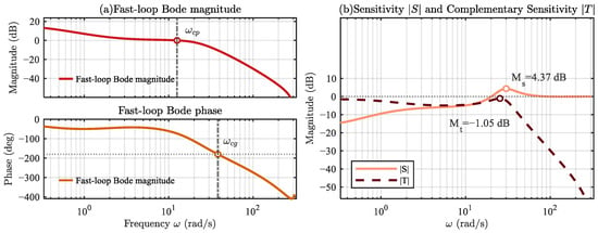
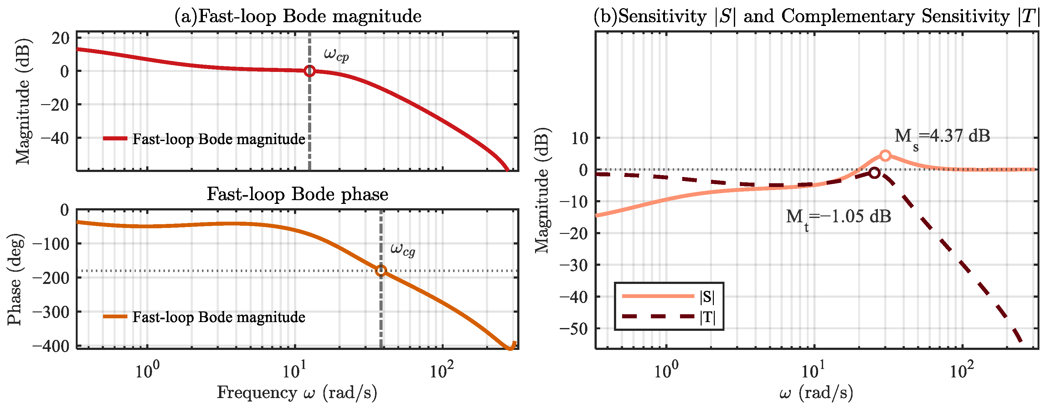
By constructing the discrete open-loop transfer function $L\left(z\right)$, the fast loop exhibits good stability characteristics. Bode plot analysis shows that the system has high DC gain within the target bandwidth, enabling rapid elimination of line-of-sight deviation.

As shown in Figure 3a, near the 0 dB crossover frequency $f_c$, the open-loop magnitude crosses 0 dB with approximately a first-order roll-off; the phase at crossover is around $-{100}^{°}$, resulting in a phase margin significantly greater than ${45}^{°}$. Thus, the system maintains sufficient stability margin even with the included sampling and transmission delays. The magnitude roll-off in the high-frequency region is faster than $-40$ dB/decade, preventing significant amplification of measurement noise. The accompanying sensitivity curve is shown in Figure 3b. The peak of $\mid S\mid$ is controlled within 6 dB, and $\mid T\mid$ shows no abnormal peaking at high frequencies, indicating that the robustness reserve in the linear domain meets the design target. The peak values of the sensitivity function $M_s$ and complementary sensitivity function $M_t$ are both kept within reasonable ranges, demonstrating the system’s good robustness to model uncertainty and avoiding excessive injection of high-frequency noise into the actuator chain. These robustness margins and sensitivity bounds were used not only for analysis, but also as acceptance criteria during controller tuning. Key parameters and Bode margin values for the fast loop are summarized in Table 4.

Figure 3. Fast loop open-loop Bode plot and sensitivity comparison plot.

Table 4. Quick metrics and implementation parameters.

Variable	GM (dB)	PM (deg)	${\mathit{\omega }}_{\mathit{c}\mathit{g}}$ (rad/s)	${\mathit{\omega }}_{\mathit{c}\mathit{p}}$ (rad/s)	${\mathit{M}}_{\mathit{s}}$ (dB)	${\mathit{M}}_{\mathit{t}}$ (dB)
Parameter	10.44	106.39	38.25	12.57	4.37	−1.05
Variable	${\mathit{T}}_{\mathit{s}\mathit{f}}$	$\mathit{\beta }$	${\mathit{K}}_{\mathit{p}}$	${\mathit{k}}_{\mathit{p}\mathit{a}}$	${\mathit{K}}_{\mathit{m}}$	$\mathit{d}$
Parameter	0.01	0.429	877	0.0012	1	1

Discrete-time stability of the linearized closed-loop system was verified using the Jury criterion. Taking the closed-loop characteristic polynomial:

$$\mathsf{\Phi }\left(z\right)=1+{\varphi }_1{z}^{-1}+\cdots +{\varphi }_n{z}^{-n}$$

(57)

$$P\left(z\right)\triangleq z^n\mathsf{\Phi }\left(z\right)=a_0{z}^n+a_1{z}^{n-1}+\cdots +a_n$$

(58)

The three necessary conditions of the Jury criterion are $\mid a_n\mid < a_0$, $P\left(1\right)>0$, $(-1{)}^{n}P(-1)>0$. Calculations yield the following:

$${\displaystyle \frac{\mid a_n\mid }{a_0}}=0.5025<1$$

(59)

$$P(1)=\sum _{k=0}^4{a}_k=0.0003135>0,$$

(60)

$${(-1)}^{n}P(-1)=\sum _{k=0}^4{a}_k{(-1)}^k=11.5404>0$$

(61)

All closed-loop poles lie within the unit circle, confirming discrete-time closed-loop stability of the linearized model.

3.2.2. Slow Loop Frequency Domain Analysis and Nonlinear Screening

To comprehensively assess the stability and reliability of the slow loop in practical engineering, this paper adopts a three-level analysis framework: linear frequency-domain margin assessment, nonlinear describing-function screening, and time-domain verification. The first level provides the local robustness baseline of the linearized feedback path, while the latter two levels are used to examine whether the dominant actuator nonlinearities may induce oscillatory behavior not captured by the linearized model.

Under the small-signal linearization assumption around the calibrated operating point, the Bode-based stability-margin analysis is first performed on the slow-loop open-loop transfer function $L\left(j\omega \right)$, providing the baseline robustness judgment for the feedback main path.

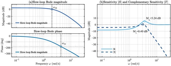
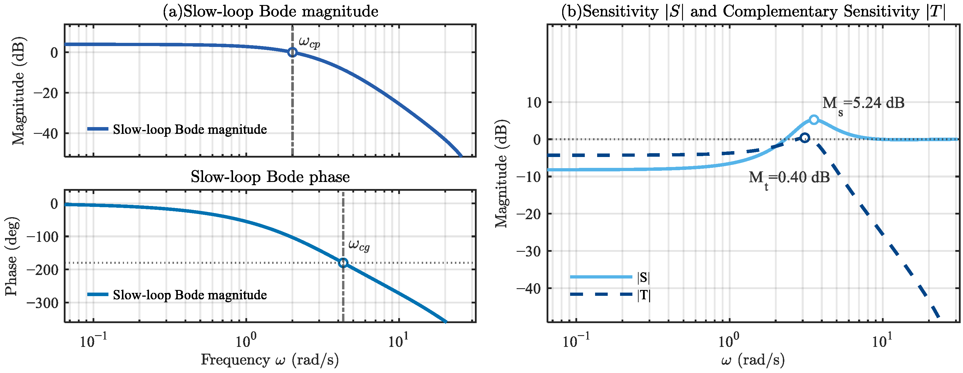
From the Bode plot in Figure 4a, it can be seen that the low frequency maintains sufficient DC gain to ensure steady-state stiffness; the mid-frequency crossover has a roll-off of approximately $-20$ to $-40$ dB/decade, with a phase margin of $\ge {40}^{°}$ at ${\omega }_{c,s}$; the high-frequency roll-off is no less than $-40$ dB/decade, avoiding the feedback of sensor noise into the actuator chain. The accompanying sensitivity curves in Figure 4b show: the peak $\mid S\mid$ is controlled within 6 dB, and $\mid T\mid$ shows no abnormal peaking at high frequencies, indicating that the linear domain robustness reserve meets the design target. Key Bode margin values are summarized in Table 5.

Figure 4. Slow loop open-loop Bode plot and sensitivity comparison plot.

Table 5. Slow loop indicators and implementation parameters.

Variable	GM (dB)	PM (deg)	${\mathit{\omega }}_{\mathit{c}\mathit{g}}$ (rad/s)	${\mathit{\omega }}_{\mathit{c}\mathit{p}}$ (rad/s)	${\mathit{M}}_{\mathit{s}}$ (dB)	${\mathit{M}}_{\mathit{t}}$ (dB)
Parameter	8.54	76.77	4.31	2.00	5.24	0.4
Variable	${\mathit{T}}_{\mathit{s}\mathit{s}}$	${\mathit{\omega }}_{\mathit{r}}$	$\mathit{f}$	${\mathit{K}}_{\mathit{p}}$	${\mathit{\tau }}_{\mathrm{act}}$	${\mathit{K}}_{\mathit{b}}$
Parameter	0.1	0.32	3494.68	5480	0.25	1

Although linear analysis provides initial stability assurance, nonlinearities present in the actual system can induce nonlinear instability phenomena such as limit cycle oscillations. Addressing the nonlinearities in the actual actuator and guidance law, a composite describing function is constructed, and the limit cycle condition is solved based on this:

$$\mid L\left(j\omega \right)N\left(A\right)\mid =1$$

(62)

$$\mathrm{a}\mathrm{r}\mathrm{g}\left(L\right(j\omega \left)N\right(A\left)\right)=-\pi$$

(63)

This paper considers three types of nonlinearities:

Dead zone $\mathrm{d}$: Uses the standard describing function:

$${\mathrm{N}}_{\mathrm{dead}}(\mathrm{A})={\displaystyle \frac{2}{\mathsf{\pi }\mathrm{A}}}(\sqrt{{\mathrm{A}}^2-{\mathrm{d}}^2}-\mathrm{d}\mathrm{a}\mathrm{r}\mathrm{c}\mathrm{c}\mathrm{o}\mathrm{s}{\displaystyle \frac{\mathrm{d}}{\mathrm{A}}}),\mathrm{A}>\mathrm{d}$$

(64)

Amplitude saturation $\pm u_{\mathrm{m}\mathrm{a}\mathrm{x}}$: Uses the classical expression $N_{\mathrm{sat}}\left(A\right)$ for a segmented sinusoidal input.

Rate limiting: Approximated by an equivalent first-order lag $N_{\dot{u}}(A,\omega )$ to account for its amplitude–frequency dependent gain compression and phase lag [27].

The composite describing function is $N(A,\omega )=N_{\mathrm{dead}}\left(A\right)N_{\mathrm{sat}}\left(A\right)N_{\dot{u}}(A,\omega )$. To avoid underestimating risk, the screening phase in this paper uses $N_{\mathrm{dead}}\cdot N_{\mathrm{sat}}$, leaving the effect of rate limiting to be covered in the time-domain review.

Discretizing on a logarithmic grid for $\omega \in [{10}^{-2},\pi /T_s)$ and a linear grid for $A\in [{0.05}^{°},{30}^{°}]$ (this paper uses $1600\times 400$ points), a dual-threshold Boolean mask is constructed:

$$\mid \hspace{0.17em}{\mid L\mid }^{-1}-N(A)\hspace{0.17em}\mid <0.02,\mid \hspace{0.17em}{\mathrm{wrap}}_{[-\pi ,\pi ]}(\mathrm{\angle }L+\pi )\hspace{0.17em}\mid <5^{°}$$

(65)

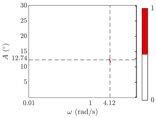
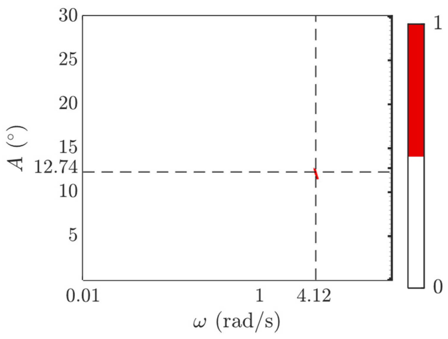
Points satisfying these conditions are marked as 1, and a candidate region Boolean map is plotted. Points satisfying these conditions are marked as 1, and a candidate region Boolean map is plotted. In Figure 5, red denotes the candidate region where both the magnitude and phase conditions in Equation (65) are simultaneously satisfied, whereas white denotes non-candidate regions.

Figure 5. Describing function limit cycle screening heat map.

Figure 5 shows that the candidate regions are very sparse, with only one prominent ‘bright spot’ solution:

$$A^{\star }\approx {12.74}^{°},{\omega }^{\star }\approx 4.12 \mathrm{rad}/\mathrm{s} (f^{\star }\approx 0.66 \mathrm{Hz},T^{\star }\approx 1.52 \mathrm{s})$$

(66)

This point is located near a strong nonlinear boundary. This result suggests a potential for small-amplitude self-oscillation when the input swing is close to ${13}^{°}$ and the frequency falls in the $0.6–0.7$ Hz region, if the nonlinear combination makes $\mid LN\mid = 1$ and the total phase is close to $-\pi$. The nonlinear constraint parameters are shown in Table 6.

Table 6. Nonlinear constraint parameter table.

Variable	$\mathit{d}$	$\pm {\mathit{u}}_{\mathbf{m}\mathbf{a}\mathbf{x}}$	$\dot{\mathit{u}}{\mathbf{\mid }}_{\mathbf{m}\mathbf{a}\mathbf{x}}\mathbf{\mid }$	Frequency Scan Range	Amplitude Scanning Range
Parameter	0.15°	10°	0.6 (rad/s)	$\omega \in [{10}^{-2},0.98\pi /T_{ss}]$ × 1600	$A\in [0.05,30]$ × 400

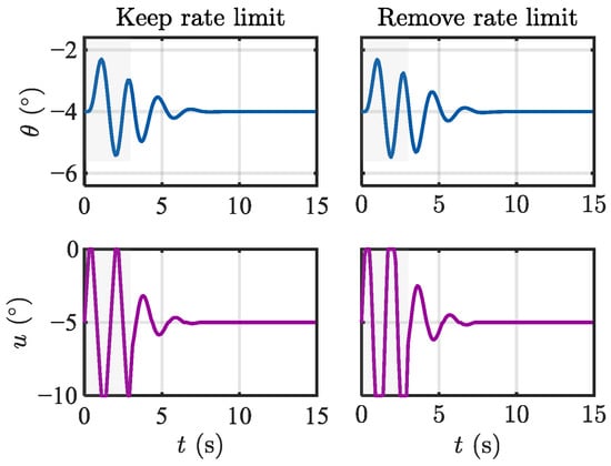
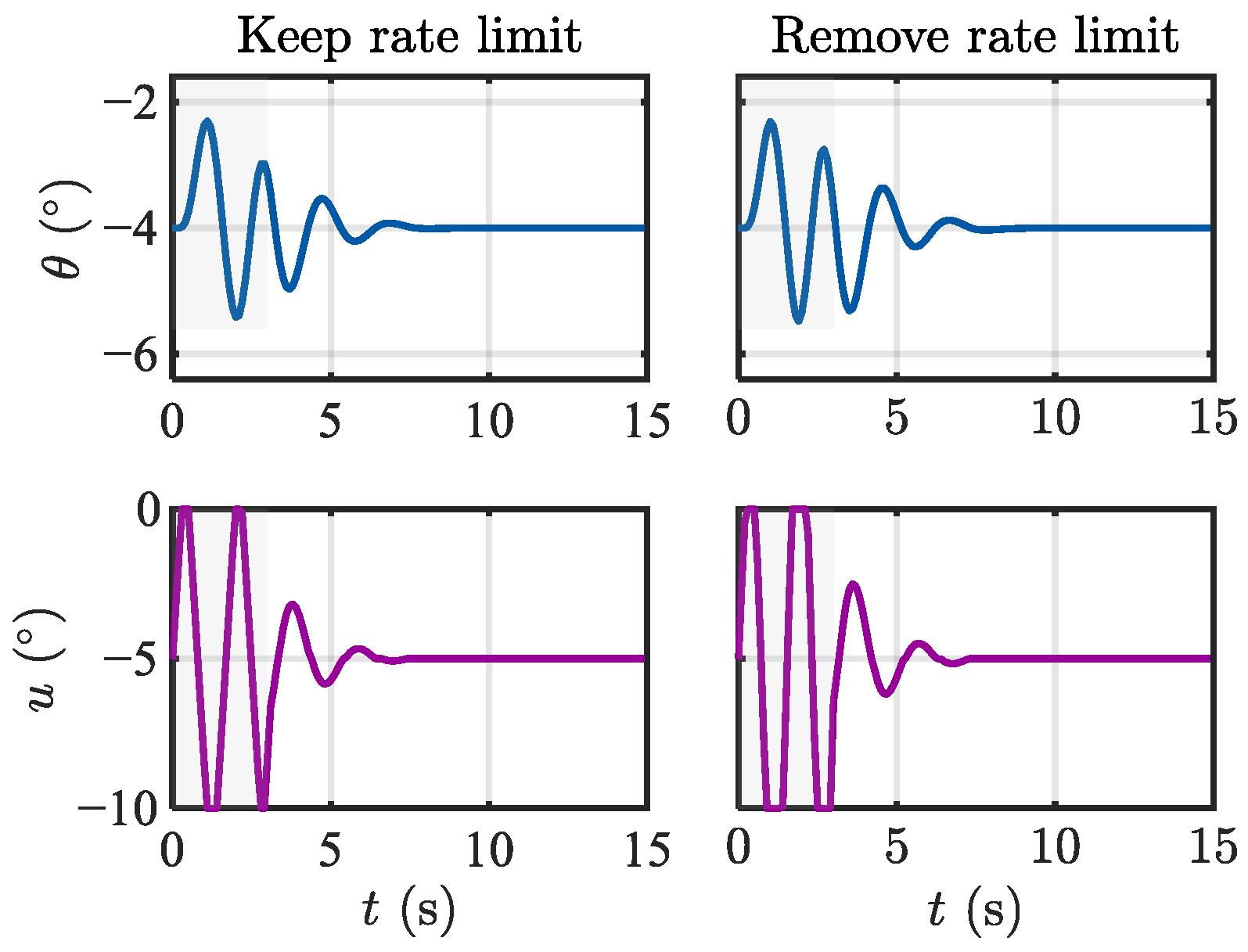
For this point, a directed excitation time-domain review was conducted: a 3-s sinusoidal excitation was injected into the closed loop just before the nonlinearities, and the free response after removing the excitation was observed under two settings: “with rate limiting” and “without rate limiting”. The results are shown in Figure 6. The envelopes of $\theta \left(t\right)$ and $u\left(t\right)$ decay rapidly in both settings, without locking into a stable oscillation, indicating that this candidate solution cannot sustain itself under the actual constraints and rate limiting.

Figure 6. Directed excitation time-domain review plot.

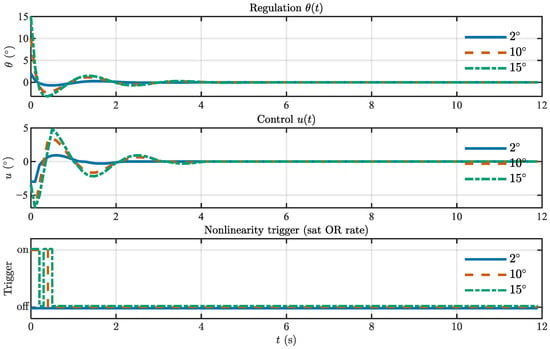
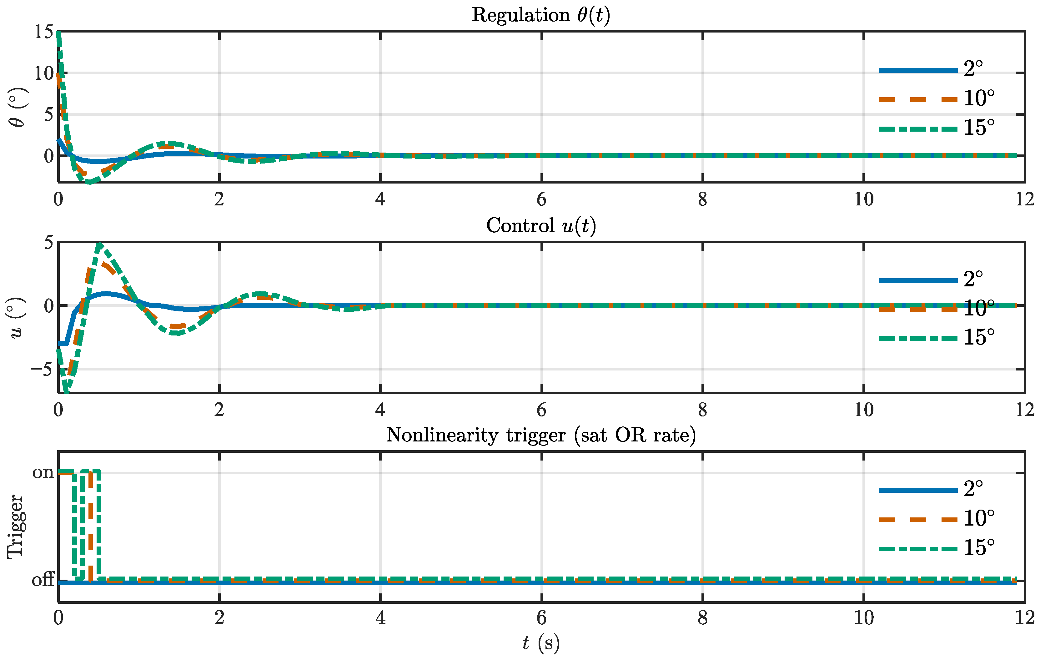
Furthermore, nulling experiments were conducted under fixed target scenarios. Figure 7 shows the response comparison for initial deviations of $2^{°}$, ${10}^{°}$, and ${15}^{°}$: the settling times are approximately 1.9 s, 2.7 s, and 2.8 s, respectively, and the maximum overshoots are about 25%, 23%, and 21%. The triggered nonlinear trajectory shows: For the $2^{°}$ case, amplitude saturation was not triggered, and rate limiting only occurred for about 0.3–0.4 s at startup; The ${10}^{°}$ and ${15}^{°}$ cases experienced brief amplitude saturation for about 0.2 s, accompanied by rate limiting for 0.4–0.5 s. Throughout the process, no narrowband self-oscillation or long-term oscillation was observed. The residual error near zero under pixel-level noise is approximately $0^{°}$.

Figure 7. Fixed-point nulling and nonlinear triggering trajectory.

The above analysis serves two purposes. First, it provides a systematic check for potential limit cycles arising from the interaction between the linear dynamics and the dominant actuator nonlinearities. Second, it verifies that the linearized model used for frequency-domain design remains a meaningful approximation of the implemented system within the intended operating envelope. The candidate limit-cycle solution suggested by the describing-function screening does not develop into sustained oscillation under the implemented constraint settings, as confirmed by the directed excitation tests and fixed-point nulling experiments. Therefore, the dominant nonlinearities do not invalidate the small-signal design within the tested operating envelope.

4. Experimental Validation and Analysis

Section 4 is designed to validate the theoretical developments in Section 2 and Section 3. Section 4.2.2 verifies the fast-loop centering and anti-jitter behavior, Section 4.2.3 validates the slow-loop delay-aware regulation and feedforward–feedback coordination during continuous extinguishment, and Section 4.3 shows that the proposed dual-loop architecture achieves smoother convergence, less redundant oscillation, and higher extinguishment efficiency than the benchmark methods.

4.1. Training and Results of the Object Detection Model

4.1.1. Dataset Construction and Augmentation

To evaluate the joint detection capability for fire sources and water-jet impact regions, we constructed a dedicated self-collected dataset named FWS (Fire & Water Stream). All images were acquired by the authors during controlled combustion and water-discharge experiments using the same experimental platform described in Section 4.2.1. The dataset contains scenes in which fire sources and water-jet impact regions appear individually or simultaneously under different backgrounds, illumination conditions, and target positions. A total of 1234 original images were collected. All images were manually annotated using LabelImg and exported in YOLO format.

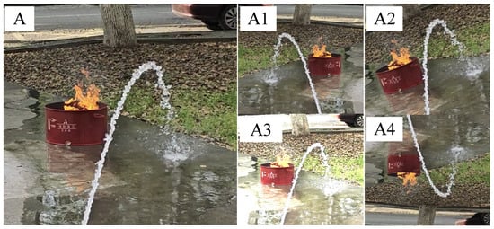
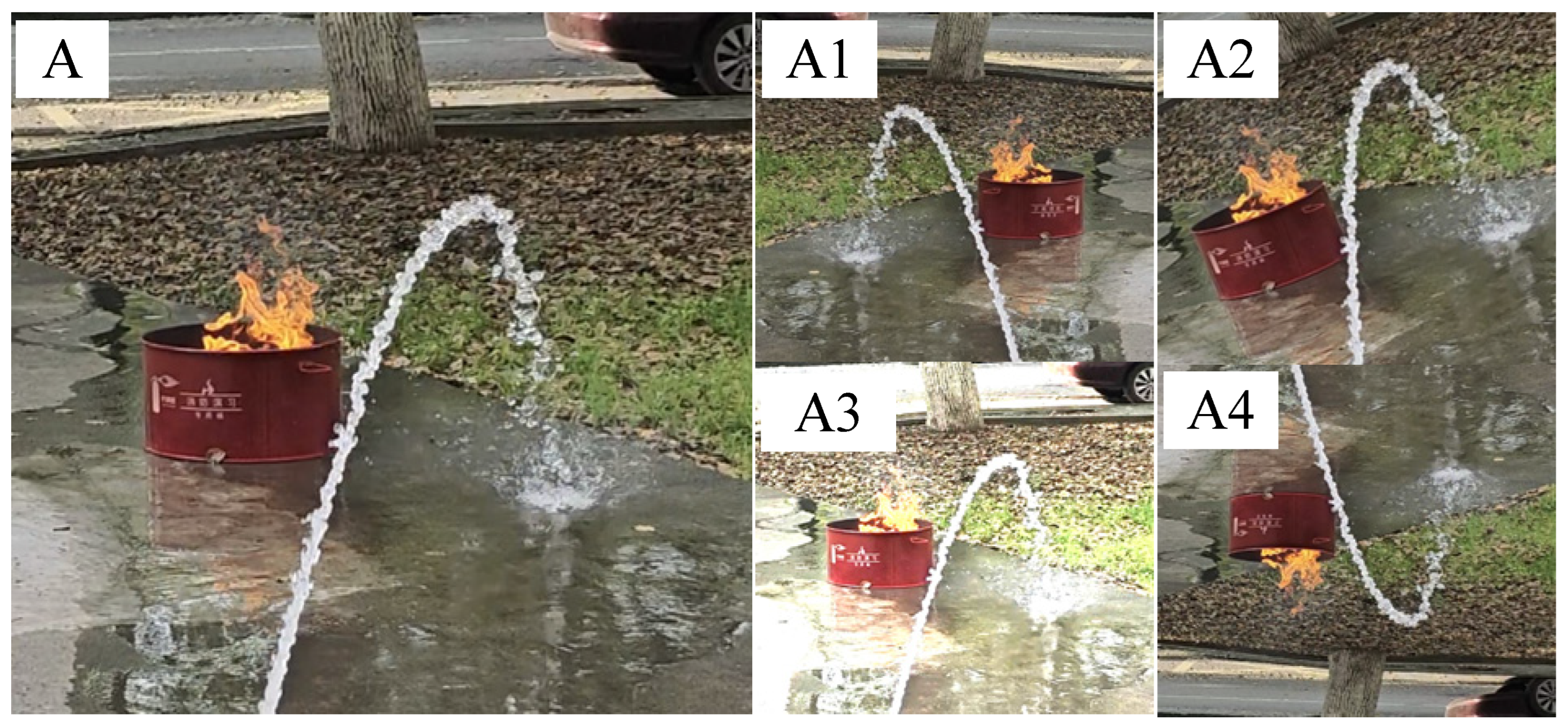
To improve robustness and reduce overfitting, standard data augmentation operations such as horizontal flipping, mirroring, and additive noise were applied, expanding the dataset to 12,396 images. The dataset was then divided into training, validation, and test sets at a ratio of 8:1:1. Figure 8 shows representative samples from our self-collected FWS dataset and their data augmentation instances, including mirroring, rotation, noise, and flipping. Here, A represents the original image, while A1, A2, A3, and A4 represent mirroring, rotation, highlighting, and vertical flipping, respectively.

Figure 8. Representative samples from the FWS dataset and data augmentation example samples.

The original FWS dataset is relatively small, and most training samples are generated by offline augmentation. Although augmentation improves robustness, it cannot replace the variability of newly collected real-scene data. Therefore, the detector is validated mainly within the data distribution covered in this study. It is expected to generalize to moderate variations similar to those represented in the dataset, but performance may degrade under larger domain shifts, such as substantially different fire scales, severe illumination changes, dense smoke, or more complex outdoor backgrounds. Future work will expand the real-scene dataset and further investigate domain adaptation when labeled data are limited [28,29].

4.1.2. Training Environment

The training environment was deployed on a Windows system with an Intel i9-13900HX CPU (Intel, Santa Clara, CA, USA), an NVIDIA GeForce RTX 4080 GPU (NVIDIA, Santa Clara, CA, USA), 10 GB of video memory, and 32 GB of system memory. The deep learning framework used was PyTorch, and TorchVision used CUDA version 12.1. The deep learning framework version was PyTorch-GPU 2.2.1+cu121, and Python version 3.8.10. The model training parameter settings are shown in Table 7.

Table 7. Training and reproducibility settings.

Parameter	Configuration	Parameter	Configuration
Input resolution	640 × 640	Epochs	500
Optimizer	SGD	Batch size	16
Weight decay	0.0005	Initial learning rate	0.001
Momentum	0.937	Learning-rate schedule	default decay
Warmup epochs	None	Training/validation/test split	8:1:1
Augmentation probability	not used (offline augmentation rather than stochastic online augmentation)	Data augmentation	horizontal flipping, mirroring, additive noise, etc.
Stopping criterion	Training ran for 500 epochs	Early stopping	not used
Split reproducibility	Fixed random seed = 0	Model selection metric	Best validation mAP50-95

4.1.3. Training Results

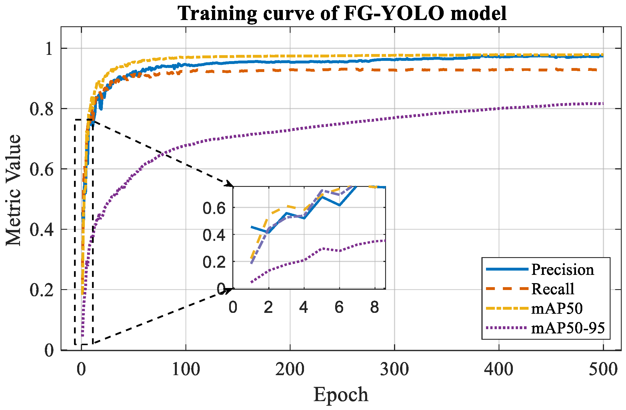
To evaluate the model’s effectiveness for the joint detection of fire sources and water-jet impact regions, standard object-detection metrics were adopted, including Precision, Recall, mean Average Precision at an IoU threshold of 0.5 (mAP50), mean Average Precision averaged over IoU thresholds from 0.50 to 0.95 (mAP50-95), and Frames Per Second (FPS). Precision is defined as the ratio of true positive detections to all positive predictions, whereas Recall is the ratio of true positive detections to all ground-truth instances. mAP is defined as the mean Average Precision over all classes, and FPS is used to measure the inference speed of the model. Let TP, FP, and FN denote the numbers of true positives, false positives, and false negatives, respectively, $N$ the number of object classes, and $A{P}_i$ the Average Precision of class $i$. Following the standard VOC/COCO evaluation definitions [30,31], Precision, Recall, and mAP are computed as follows:

$$\mathrm{P}\mathrm{r}\mathrm{e}\mathrm{c}\mathrm{i}\mathrm{s}\mathrm{i}\mathrm{o}\mathrm{n}={\displaystyle \frac{\mathrm{T}\mathrm{P}}{\mathrm{T}\mathrm{P}+\mathrm{F}\mathrm{P}}}$$

(67)

$$\mathrm{R}\mathrm{e}\mathrm{c}\mathrm{a}\mathrm{l}\mathrm{l}={\displaystyle \frac{\mathrm{T}\mathrm{P}}{\mathrm{T}\mathrm{P}+\mathrm{F}\mathrm{N}}}$$

(68)

$$\mathrm{m}\mathrm{A}\mathrm{P}={\displaystyle \frac{\sum _{\mathrm{n}=1}^{\mathrm{N}} {\int }_0^1 {\mathrm{P}\mathrm{r}\mathrm{e}\mathrm{c}\mathrm{i}\mathrm{s}\mathrm{i}\mathrm{o}\mathrm{n}}_{\mathrm{n}}\mathrm{d}\left({\mathrm{R}\mathrm{e}\mathrm{c}\mathrm{a}\mathrm{l}\mathrm{l}}_{\mathrm{n}}\right)}{\mathrm{N}}}$$

(69)

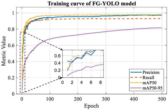
The training curves for Precision, Recall, mAP50, and mAP50-95 are shown in Figure 9, and the quantitative results are listed in Table 8. The FG-YOLO model achieved outstanding performance on the dual-detection task: for fire source detection, $\mathrm{P}\mathrm{r}\mathrm{e}\mathrm{c}\mathrm{i}\mathrm{s}\mathrm{i}\mathrm{o}\mathrm{n}$ = 97.9%, R = 92.9%, mAP50 = 97.6%, and mAP50-95 = 83.6%; for water-jet detection, $\mathrm{P}\mathrm{r}\mathrm{e}\mathrm{c}\mathrm{i}\mathrm{s}\mathrm{i}\mathrm{o}\mathrm{n}$ = 96.5%, R = 94.5%, mAP50 = 98.4%, and mAP50-95 = 79.3%. Both tasks ran at an inference speed of 58 FPS on the NVIDIA GeForce RTX 4080 GPU, satisfying real-time requirements. The model’s robust and stable recognition of water-jet landing points effectively addresses the technical challenge of synchronous fire-and-water detection in closed-loop extinguishing systems, laying a solid foundation for dynamic fire source tracking and precise firefighting.

Figure 9. Training curves of Precision, Recall, mAP50, and mAP50-95 for the FG-YOLO model.

Table 8. FG-YOLO Detection Results on the FWS Test Set.

Category	Precision (%)	Recall (%)	mAP50 (%)	mAP50-95 (%)	FPS
All	97.2	92.9	98.0	81.5	58
Fire	97.9	92.9	97.6	83.6	58
Water-jet	96.5	94.5	98.4	79.3	58

4.2. Experimental Verification of Automatic Water Cannon Fire Extinguishing System

To evaluate the system under realistic conditions, we conducted a series of controlled open-site experiments. These experiments demonstrated the system’s performance in fire-source detection, localization accuracy, and dynamic jet adjustment during simulated fire scenarios. Because no hydrant was available, we used a pump and hose attached to the cannon to simulate the jet.

4.2.1. Experimental Setup

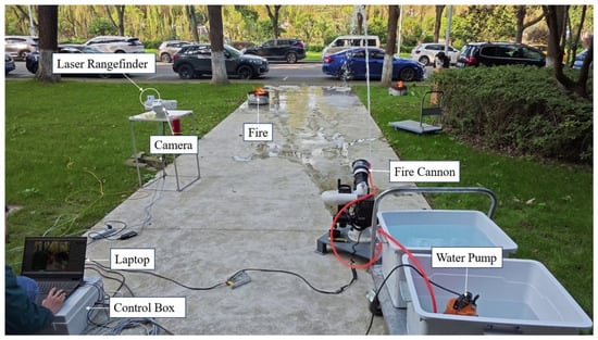
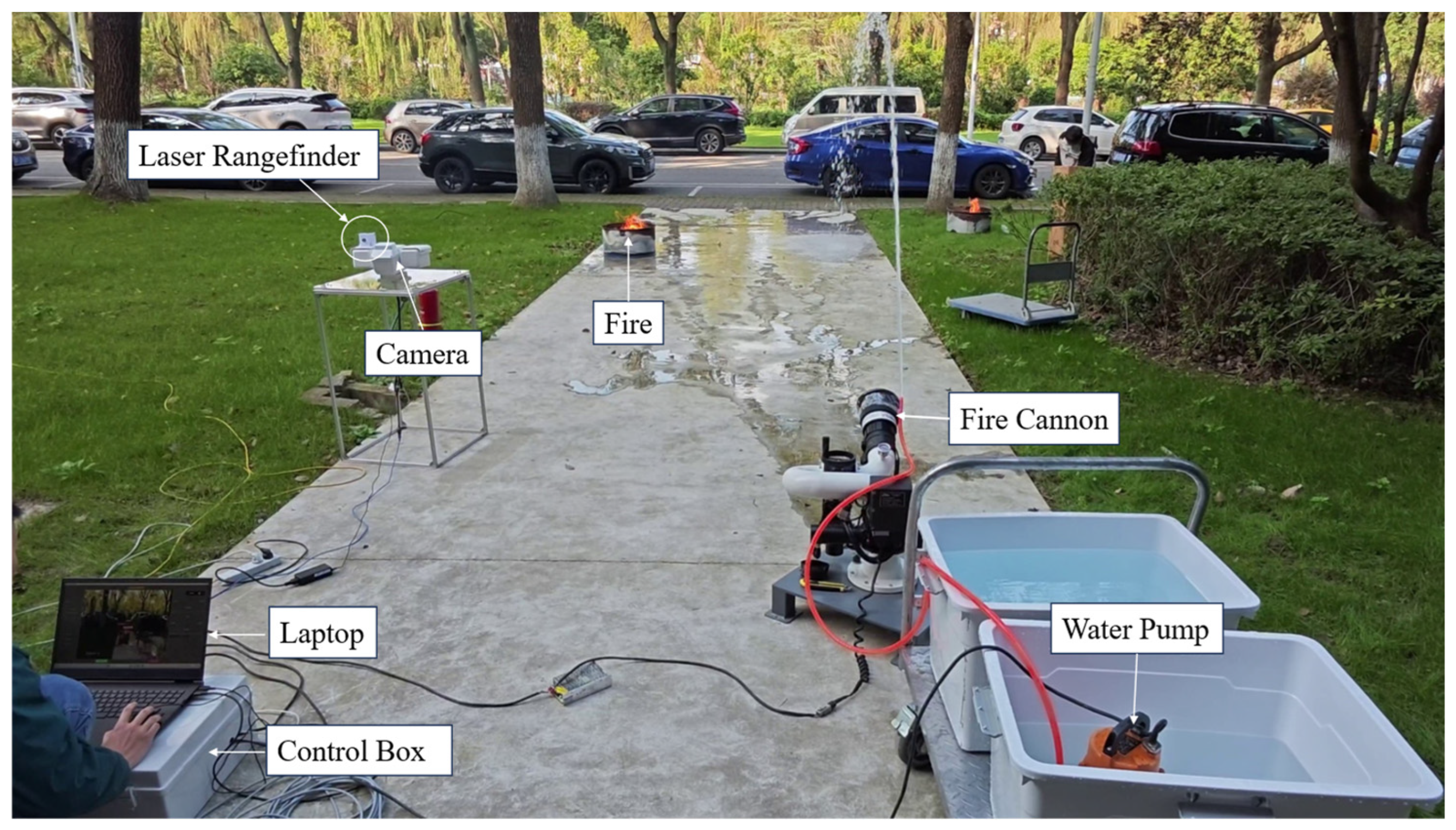
The study utilized a flat, open site with solid concrete paving to ensure stability during fire water cannon operation. The deployment layout is shown in Figure 10, with corresponding hardware specifications provided in Table 9.

Figure 10. Experimental site.

Table 9. Experimental hardware specifications.

Equipment	Model/Specification	Manufacturer (City, Country)	Key Parameters
Camera	DS-2TD5566T-7	Hikvision, Shanghai, China	Field of View: H 360°, V −90° to +90°; Resolution Ratio: 2560 × 1440.
PLC Control Box	Siemens S7-200	Siemens, Shanghai, China	Interfaces: RS-485/Ethernet; Operating Voltage: 24 V DC.
Fire Water Cannon	PSKD10/80WB-D-3680	Furuide Electronic, Shanghai, China	Horizontal: 165° each direction (330° total); Vertical: −15° to +85°.
Fire Pit	Custom Stainless-Steel	Changhong Security Factory, Shanghai, China	Diameter: 58 cm; Height: 30 cm; Fuel: Wood.
Laser Rangefinder	SW-LDS100DA	Jiuguan Measuring Instrument Co., Ltd., Shanghai, China	Range: 0.2–100 m.
Computer	17-ck2002TX	HP, Shanghai, China	CPU: i9-13900HX; GPU: RTX 4080.

4.2.2. Aiming Tracking Algorithm Test

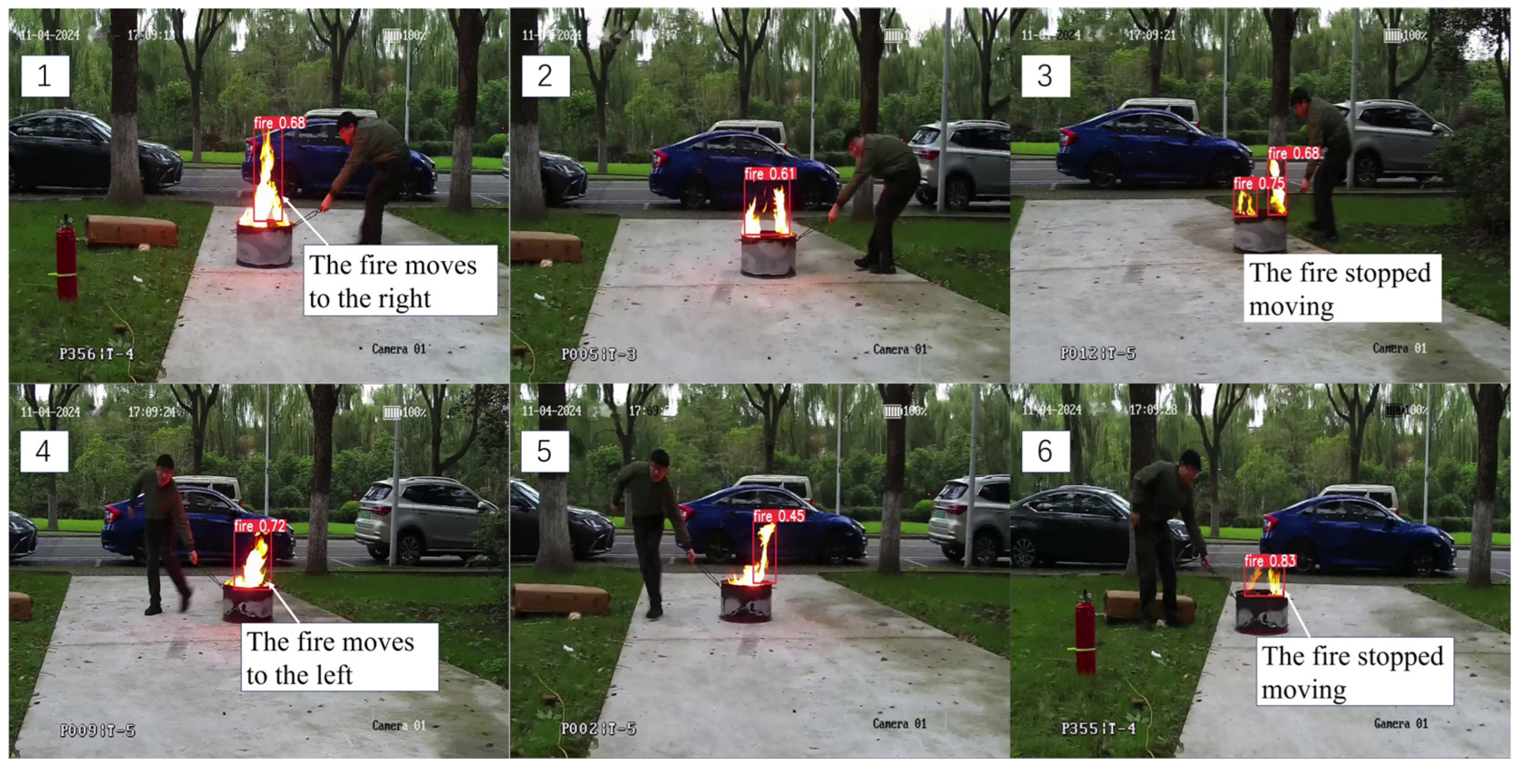
This experiment tested the system’s ability to dynamically track fire sources using visual feedback. After FG-YOLO detects a fire source, the system computes the bounding-box centroid $P_f={(x}_f,y_f)$. Using the cross-coordinate quadrant positioning algorithm (Section 2.2.2), it then generates control commands to adjust the pan–tilt unit. During the alignment phase, the controller moves the camera until the fire source’s bounding-box centroid lies inside a preset tolerance box around the image center. At that point the fire source centroid is aligned with the image center.

During the experiment, an operator moved the fire source while the system operated. As shown in Figure 11, the system successfully detected these position changes in real time and adjusted the camera accordingly. This maintained alignment between the camera and the moving fire target.

Figure 11. Aiming and tracking algorithm test. Note: Frames (1)–(3) show rightward target motion followed by stopping, and Frames (4)–(6) show leftward target motion followed by stopping; the camera is adjusted in real time to maintain target alignment.

The experiments demonstrate that the proposed aiming-and-tracking algorithm enables stable, real-time tracking of moving fire sources in dynamic environments. This provides an important directional reference for the aiming of subsequent water cannon shots.

4.2.3. Water Cannon Fire Extinguishing Experiment

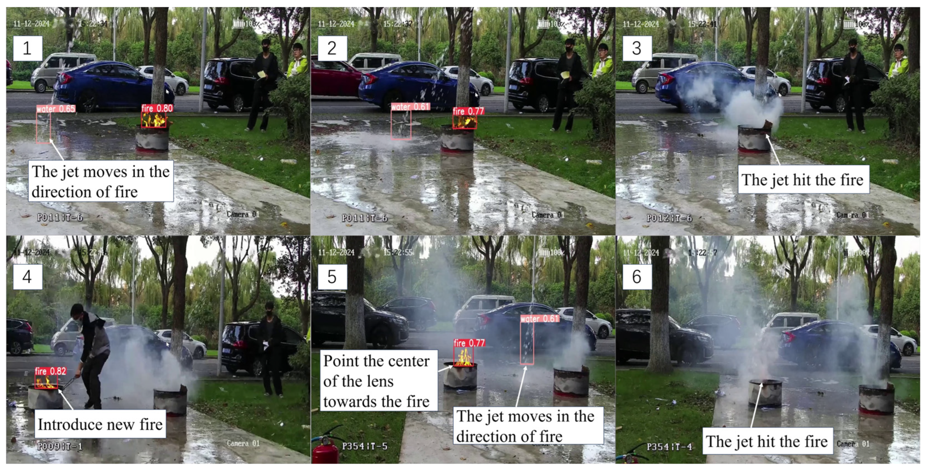
To verify the closed-loop firefighting capability of the automatic water cannon and evaluate its real-time correction of the water-jet impact point and final extinguishing effectiveness in a dynamic environment, this section designs a continuous fire suppression experiment. As shown in Figure 12, the first fire source is extinguished within 8 s, after which a second fire source is immediately ignited. The system seamlessly handles fire source re-identification, target switching, and closed-loop real-time correction of the jet impact point without control interruption or manual intervention, successfully locating and suppressing the second target within 11 s, for a total continuous mission duration of 22 s (including 3 s of re-ignition time).

Figure 12. Continuous fire extinguishing process. Note: Frames (1)–(3) show the suppression of the first fire, and Frames (4)–(6) show the introduction and suppression of the second fire.

The results indicate that the system maintains stable control and error convergence in multi-target, continuous operation scenarios, demonstrating effective sustained firefighting capability and task succession ability.

4.3. Comparative Experiments and Performance Analysis

To systematically evaluate the performance advantages of the proposed dual closed-loop control architecture, comparative experiments were conducted under identical hardware platforms, visual perception modules, and testing procedures. All experiments utilized the same fire source centroid and jet stream impact point pixel coordinates output by the visual module, with comparisons made solely based on differences in control strategies to ensure consistency in experimental conditions. The experimental environment is as described in Section 4.2.1, with consistent fire source positions and initial conditions to eliminate external variable interference.

4.3.1. Benchmark Methods and Evaluation Metrics

1.

Benchmark Methods

Three control strategies were considered in the comparative evaluation. Their main differences lie in the control architecture and the configurations of key algorithmic modules, as summarized in Table 10.

Table 10. Benchmark Controller Configurations.

Method	Command Limiting	Anti-Windup	Filtering	Prediction	Trajectory Smoothing
Baseline1	√	×	×	×	×
Baseline2	√	√	√	×	×
Ours	√	√	√	√	√

Note: √ indicates that the corresponding module is included in the controller, whereas × indicates that it is not included.

Coupled proportional baseline (Baseline 1): This benchmark represents a direct coupled control strategy in which the fire-centering error and the jet-impact correction error are combined to generate control commands without dynamic decoupling, prediction, or trajectory shaping. It is used as a simple engineering reference scheme reflecting direct error-driven control.

Incremental-PID baseline (Baseline 2): This benchmark represents a conventional engineering feedback-control scheme based on incremental PID with command limiting, basic anti-windup treatment, and filtering. It is included because PID-type controllers remain among the most widely adopted standard approaches in practical motion and process control systems.

Proposed method (Ours): The control strategy proposed in this paper is adopted. Under actuator constraints and perception–actuation frequency mismatch, it incorporates prediction, feedback correction, command limiting, and command trajectory shaping to improve convergence speed and reduce residual fluctuations.

Baseline 1 and Baseline 2 were designed as two progressively strengthened same-platform benchmarks. Baseline 1 serves as a minimal coupled error-driven reference, intended to reflect the limitations of a scheme without dynamic decoupling, prediction, or trajectory shaping. Baseline 2 was then developed from this reference by adding incremental PID regulation, basic anti-windup treatment, and filtering according to standard feedback-control practice [14,15]. This progressive benchmark construction was adopted so that the effects of dynamic decoupling, delay-aware prediction, and command-trajectory smoothing in the proposed method on overall control performance could be identified more clearly.

2.

Evaluation Metrics

To facilitate a unified description, the definition of the error signal $e_p$ is first provided. Let the fire source centroid detected in the $k$-th frame be ${\mathrm{p}}_f[k]=(x_f[k],y_f[k])$, and the jet stream impact point be ${\mathrm{p}}_w[k]=(x_w[k],y_w[k])$. The jet alignment error is defined as the pixel-wise Euclidean distance between them in the image plane:

$$e_p[k]=\parallel {\mathrm{p}}_w[k]-{\mathrm{p}}_f[k]{\parallel }_2=\sqrt{\left(x_w[k]-x_f[k]{)}^2+(y_w[k]-y_f[k]{)}^2\right.}$$

(70)

The following four key metrics are used for evaluation to objectively quantify the control system performance:

(1)

Normalized Total Variation of Error ($NT{V}_e$): To measure the average fluctuation intensity of the error during convergence, the Normalized Total Variation is defined within an evaluation window $W$:

$$NT{V}_e={\displaystyle \frac{1}{\mid W\mid -1}}\sum _{k\in W,k>k_s}\mid e_p[k]-e_p[k-1]\hspace{0.17em}\mid$$

(71)

where $e_p[k]$ is the impact point alignment error in the $k$-th frame, $k_s$ is the starting frame index of the window, and $\mid W\mid$ is the number of samples within the window. A smaller $NT{V}_e$ indicates smoother error variation and weaker jitter.

This can also be expressed as $NT{V}_e={\displaystyle \frac{T{V}_e}{\mid W\mid -1}}$, where $T{V}_e$ is the total variation. A smaller $NT{V}_e$ signifies less average fluctuation per sampling step.

(2)

Excess Ripple Ratio ($r_{excess}$): To further characterize redundant back-and-forth error oscillations, the net error change within the window is defined as:

$$Ne{t}_e=\mid e_p\left[k_e\right]-e_p\left[k_s\right]\hspace{0.17em}\mid$$

(72)

where $k_e$ is the ending frame index of the window. Let

$$T{V}_{excess}=\sum _{k\in W,k>k_s}\mid e_p[k]-e_p[k-1]\mid -Ne{t}_e$$

(73)

The excess ripple ratio is then:

$$r_{excess}={\displaystyle \frac{T{V}_{excess}}{\sum _{k\in W,k>k_s}\mid e_p\left[k\right]-e_p[k-1]\hspace{0.17em}\mid }}$$

(74)

A smaller $r_{excess}$ indicates fewer repeated oscillations. When $r_{excess}=0$, the error changes monotonically within the window.

(3)

Task Success Rate ($S$): The fire extinguishment success rate measures the reliability of the system in completing autonomous firefighting tasks. Given a total number of trials $M$ and the number of successful extinguishment trials $N$, the success rate is defined as:

$$S={\displaystyle \frac{N}{M}}\times 100\%$$

(75)

A trial was counted as successful if the system autonomously completed fire suppression under the prescribed test procedure without manual intervention; a trial was counted as failed if extinguishment could not be completed within the trial window or manual intervention was required.

(4)

Extinguishment Time $\left(T,\mu \pm SD\right)$: Extinguishment time is defined as the time from the start of autonomous control to complete fire-source extinction. Each method is evaluated in five repeated trials under the same initial conditions. The reported extinguishment time is given as mean ± standard deviation and is calculated only from successful trials; failed trials are not included in this statistic and are instead accounted for in the success rate.

For the repeated comparative experiments, the normalized total variation and excess ripple ratio were first computed for each individual trial over the same evaluation window and then summarized across the five repeated trials in the form of mean ± standard deviation. For the task success rate, the point estimate is reported together with a 95% confidence interval computed by the Wilson score interval. For extinguishment time, the value is reported as mean ± standard deviation over successful trials only.

4.3.2. Result Analysis

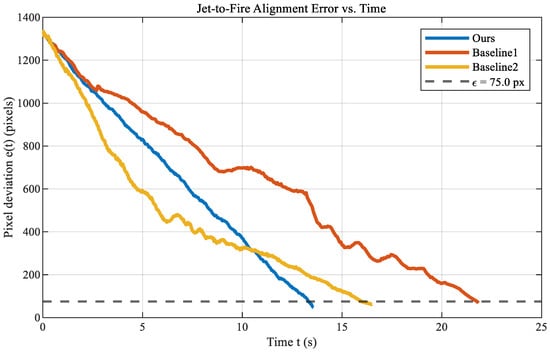
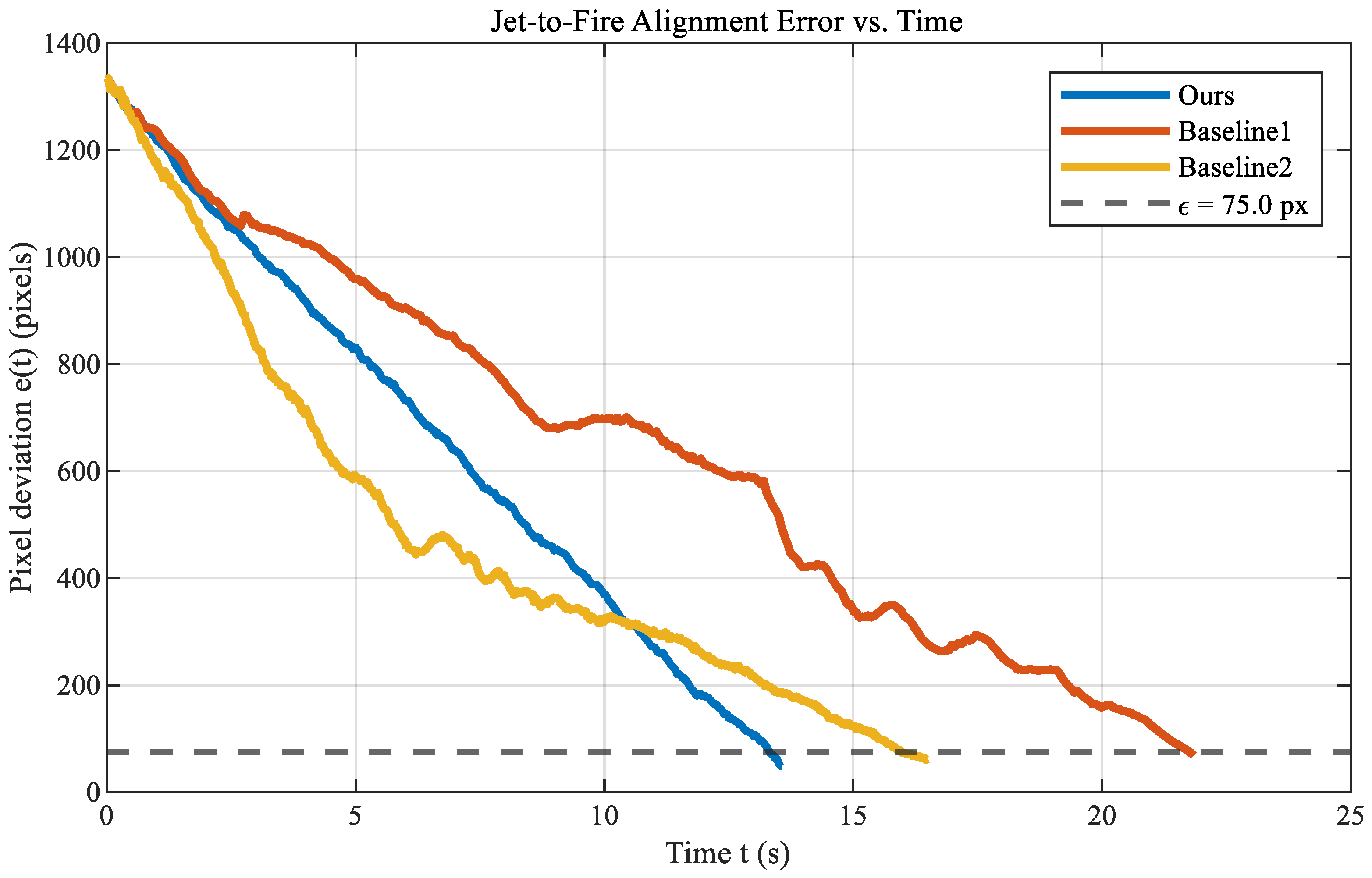
Under identical experimental conditions, each control strategy was evaluated in five repeated trials. Table 11 reports the normalized total variation and excess ripple ratio in the form of mean ± SD across repeated trials, the task success rate together with its 95% confidence interval, and the extinguishment time in the form of mean ± SD over successful trials only. The impact-point error curves for a representative trial are shown in Figure 13.

Table 11. Quantitative Comparison Results of the Three Control Strategies.

Method	$\mathit{N}\mathit{T}{\mathit{V}}_{\mathit{e}}$ (Mean ± SD)	${\mathit{r}}_{\mathbf{e}\mathbf{x}\mathbf{c}\mathbf{e}\mathbf{s}\mathbf{s}}$ (Mean ± SD)	S/% (95% CI)	T (Mean ± SD)/s
Baseline1	4.53 ± 0.23	0.37 ± 0.05	60 (23.1–88.2)	23.76 ± 2.11
Baseline2	3.89 ± 0.20	0.24 ± 0.03	100 (56.6–100)	15.83 ± 1.35
Ours	3.22 ± 0.11	0.08 ± 0.02	100 (56.6–100)	13.55 ± 0.38

Note: $NT{V}_e$ and $r_{\mathrm{e}\mathrm{x}\mathrm{c}\mathrm{e}\mathrm{s}\mathrm{s}}$ are reported as mean ± SD across the five repeated trials. Extinguishment time is reported as mean ± SD over successful trials only; failed trials are excluded from this statistic and are reflected separately by the success rate. The 95% confidence interval of the success rate is computed using the Wilson score interval.

Figure 13. Impact Point Alignment Error Variation Curves Over Time.

Based on Figure 13 and Table 11, Baseline1 showed the slowest convergence and the largest error ripple during the approach phase. The proposed method succeeded in all 5 trials, as did Baseline2, whereas Baseline1 succeeded in 3 of 5 trials. In the two failed Baseline1 trials, repeated oscillation and stagnation prevented the jet impact from remaining near the fire source within the prescribed test window.

Relative to Baseline2, the proposed method reduced the mean normalized total variation from 3.89 to 3.22 (17.2%) and the excess ripple ratio from 0.24 to 0.08 (66.7%). Relative to Baseline1, the reductions were 28.9% and 78.4%, respectively, indicating smoother convergence and fewer redundant back-and-forth corrections.

The proposed method also achieved the shortest extinguishment time, 13.55 ± 0.38 s, compared with 15.83 ± 1.35 s for Baseline2 and 23.76 ± 2.11 s for Baseline1. This corresponds to reductions of 14.4% and 43.0%, respectively. The smaller standard deviation further suggests better repeatability across repeated trials.

5. Conclusions

This study developed and experimentally validated a vision-guided dual-loop control framework for a fire-truck-mounted electric water cannon. By separating fast fire-source centering from slow jet-impact regulation, the proposed architecture addresses the perception–actuation bandwidth mismatch of high-inertia cannon systems and reduces redundant oscillation under high-rate visual feedback and actuator constraints.

In the fast loop, a lightweight visual-servoing strategy enables rapid target centering. In the slow loop, delay-aware prediction, feedback correction, and command shaping generate smooth executable pan–tilt references. Frequency-domain models were established for both loops, and the corresponding stability and robustness were evaluated under the considered delay and actuator-bandwidth constraints.

Open-site experiments, including target tracking, continuous extinguishment, and comparative tests, showed that the proposed system can autonomously track and suppress fires under the tested conditions. Compared with the benchmark controllers, it achieved smoother error convergence and shorter extinguishment time.

Overall, the results demonstrate the feasibility of the proposed dual-loop architecture under the tested conditions; however, several limitations remain. The original FWS dataset is relatively small, and much of the final training data comes from offline augmentation. The experiments were conducted mainly under controlled open-site conditions with limited fire scenarios. In addition, wind disturbance, water-pressure variation, and dynamic fire behavior were not explicitly examined, and the system was validated on an experimental platform rather than a fully integrated truck platform. Broader comparisons with other related systems have also not yet been conducted. Future work will therefore focus on expanding the real-scene dataset, increasing scenario diversity, testing on a real truck platform, and carrying out broader comparative validation under more representative conditions.

References

- Jiangsu Provincial Fire and Rescue Corps. The State Fire and Rescue Administration Held a Routine Press Conference. Available online: https://js.119.gov.cn/202501/jsxfww-menu-zxft-zxftlb_c_a9f51911e874498586b7.html (accessed on 26 January 2025). (In Chinese)
- Hall, S. Fire Loss in the United States During 2024; NFPA Research: Quincy, MA, USA, 2024; Available online: https://content.nfpa.org/-/media/Project/Storefront/Catalog/Files/Research/NFPA-Research/US-Fire-Problem/osFireLoss.pdf (accessed on 25 March 2026).
- National Fire Protection Association. United States Firefighter Injuries. Available online: https://www.nfpa.org/education-and-research/research/nfpa-research/fire-statistical-reports/firefighter-injuries-in-the-united-states (accessed on 25 March 2026).
- Kang, B.H.; Lee, S.C. Tele-operation system of unmanned fire truck for real-time fire suppression. Int. J. Internet Broadcast. Commun. 2022, 22, 1–6. [Google Scholar]
- Jin, Y.C.; Zang, C.H. A design of water cannon control system with remote control function and automatic mode. IOP Conf. Ser. Mater. Sci. Eng. 2019, 569, 042035. [Google Scholar] [CrossRef] [Scilit]
- Panwar, A.; Azam, M.; Bansal, N.; Bhateja, V.; Pal, S. Broad study on automated firefighting vehicle powered by Arduino. In Proceedings of the International Conference on Frontiers of Intelligent Computing: Theory and Applications, London, UK, 6–7 June 2024; Springer Nature: Singapore, 2024; pp. 89–101. [Google Scholar] [CrossRef] [Scilit]
- GB 51427—2021; Ministry of Housing and Urban-Rural Development, State Administration for Market Regulation. Technical Standard for Automatic Tracking and Positioning Jet Fire Extinguishing System. China Planning Press: Beijing, China, 2021. (In Chinese)
- Xin, Y.; Thumuluru, S.; Jiang, F.; Yin, R.; Yao, B.; Zhang, K.; Liu, B. An Experimental Study of Automatic Water Cannon Systems for Fire Protection of Large Open Spaces. Fire Technol. 2014, 50, 233–248. [Google Scholar] [CrossRef] [Scilit]
- Fujita, J.; Amano, H.; Ohno, K.; Tadokoro, S. Development of firefighting robot system applicable to petroleum complex fires. In Proceedings of the 2020 JSME Conference on Robotics and Mechatronics, Kanazawa, Japan, 27–30 May 2020. 2A1-A02. [Google Scholar]
- Kent Fire and Rescue Service. Firefighting Robot Deployed to Help Tackle Large Blazes. Available online: https://www.kent.fire-uk.org/news/firefighting-robot-deployed-help-tackle-large-blazes (accessed on 25 March 2026).
- Yao, J.; Lei, J.; Zhou, J.; Liu, C. FG-YOLO: An improved YOLOv8 algorithm for real-time fire and smoke detection. Signal Image Video Process. 2025, 19, 346. [Google Scholar] [CrossRef] [Scilit]
- Chaumette, F.; Hutchinson, S. Visual servo control. I. Basic approaches. IEEE Robot. Autom. Mag. 2006, 13, 82–90. [Google Scholar] [CrossRef] [Scilit]
- Zhang, Z. A Flexible New Technique for Camera Calibration. IEEE Trans. Pattern Anal. Mach. Intell. 2000, 22, 1330–1334. [Google Scholar] [CrossRef] [Scilit]
- Franklin, G.F.; Powell, J.D.; Workman, M.L. Digital Control of Dynamic Systems, 2nd ed.; Addison-Wesley: Reading, MA, USA, 1990. [Google Scholar]
- Skogestad, S.; Postlethwaite, I. Multivariable Feedback Control: Analysis and Design, 2nd ed.; Wiley: Chichester, UK, 2005. [Google Scholar]
- Wang, M.; Buticchi, G.; Li, J.; Gu, C.; Gerada, D.; Degano, M.; Xu, L.; Li, Y.; Zhang, H.; Gerada, C. Decoupled discrete current control for AC drives at low sampling-to-fundamental frequency ratios. IEEE J. Emerg. Sel. Top. Power Electron. 2022, 11, 1358–1369. [Google Scholar] [CrossRef] [Scilit]
- Deng, Y.; Léchappé, V.; Moulay, E.; Chen, Z.; Liang, B.; Plestan, F.; Han, Q.L. Predictor-based control of time-delay systems: A survey. Int. J. Syst. Sci. 2022, 53, 2496–2534. [Google Scholar] [CrossRef] [Scilit]
- Jiao, X.; Yang, Q.; Xu, B. Hybrid intelligent feedforward-feedback pitch control for VSWT with predicted wind speed. IEEE Trans. Energy Convers. 2021, 36, 2770–2781. [Google Scholar] [CrossRef] [Scilit]
- Khodarahmi, M.; Maihami, V. A review on Kalman filter models. Arch. Comput. Methods Eng. 2023, 30, 727–747. [Google Scholar] [CrossRef] [Scilit]
- Blair, W.D. Design of Nearly Constant Velocity Track Filters for Tracking Maneuvering Targets. In Proceedings of the 11th International Conference on Information Fusion, Cologne, Germany, 30 June–3 July 2008; pp. 1–7. [Google Scholar]
- Zhu, J.; Li, W.; Lin, D.; Zhao, G. Study on Water Jet Trajectory Model of Fire Monitor Based on Simulation and Experiment. Fire Technol. 2019, 55, 773–787. [Google Scholar] [CrossRef] [Scilit]
- Hou, X.; Cao, Y.; Mao, W.; Wang, Z.; Yuan, J. Models for Predicting the Jet Trajectory and Intensity Drop Point of Fire Monitors. Fluid Dyn. Mater. Process. 2021, 17, 859–869. [Google Scholar] [CrossRef] [Scilit]
- Lin, Y.; Ji, W.; He, H.; Chen, Y. Two-Stage Water Jet Landing Point Prediction Model for Intelligent Water Shooting Robot. Sensors 2021, 21, 2704. [Google Scholar] [CrossRef] [Scilit] [PubMed]
- Heo, H.-J.; Son, Y.; Kim, J.-M. A Trapezoidal Velocity Profile Generator for Position Control Using a Feedback Strategy. Energies 2019, 12, 1222. [Google Scholar] [CrossRef] [Scilit]
- Khalil, H.K. Nonlinear Systems, 3rd ed.; Prentice Hall: Upper Saddle River, NJ, USA, 2002. [Google Scholar]
- Richard, J.-P. Time-delay systems: An overview of some recent advances and open problems. Automatica 2003, 39, 1667–1694. [Google Scholar] [CrossRef] [Scilit]
- Gelb, A.; Vander Velde, W.E. Multiple-Input Describing Functions and Nonlinear System Design; McGraw-Hill: New York, NY, USA, 1968. [Google Scholar]
- Wang, S. Domain-adaptive faster R-CNN for non-PPE identification on construction sites from body-worn and general images. Sci. Rep. 2026, 16, 4793. [Google Scholar] [CrossRef] [Scilit] [PubMed]
- Wang, S. Domain adaptation using transformer models for automated detection of exterior cladding materials in street view images. Sci. Rep. 2025, 16, 2696. [Google Scholar] [CrossRef] [Scilit] [PubMed]
- Everingham, M.; Van Gool, L.; Williams, C.K.; Winn, J.; Zisserman, A. The pascal visual object classes (voc) challenge. Int. J. Comput. Vis. 2010, 88, 303–338. [Google Scholar] [CrossRef] [Scilit]
- Lin, T.Y.; Maire, M.; Belongie, S.; Hays, J.; Perona, P.; Ramanan, D.; Dollár, P.; Zitnick, C.L. Microsoft coco: Common objects in context. In Proceedings of the European Conference on Computer Vision, Zurich, Switzerland, 6–12 September 2014; Springer International Publishing: Cham, Switzerland, 2014; pp. 740–755. [Google Scholar]
Disclaimer/Publisher’s Note: The statements, opinions and data contained in all publications are solely those of the individual author(s) and contributor(s) and not of MDPI and/or the editor(s). MDPI and/or the editor(s) disclaim responsibility for any injury to people or property resulting from any ideas, methods, instructions or products referred to in the content. |
© 2026 by the authors. Licensee MDPI, Basel, Switzerland. This article is an open access article distributed under the terms and conditions of the Creative Commons Attribution (CC BY) license.