


Abstract
Unmanned aerial vehicles (UAVs) for environmental monitoring typically rely on embedded platforms with limited computational capacity, which constrains the deployment of highly accurate yet computationally demanding object-detection models. To address this challenge and enable real-time image recognition under resource limitations, this study develops three lightweight neural network architectures based on the YOLOv11 framework. The proposed designs aim to significantly reduce computational complexity and parameter count while maintaining stable and reliable detection performance, thereby improving inference efficiency and deployment flexibility on UAV platforms. YOLOv11-M is selected as the baseline model due to its favorable trade-off between detection accuracy and inference speed. Three lightweight strategies are then proposed and evaluated. First, a Ghost Convolution approach replaces portions of standard convolution with low-cost linear operations, effectively reducing both parameter size and computational overhead during feature extraction. Second, MobileNetV4 is employed as the backbone network; its optimized bottleneck structures and attention mechanisms enable substantial model compression without compromising recognition performance. Third, a MobileOne architecture with reparameterization is introduced, in which multi-branch structures enhance feature learning during training and are subsequently merged into a single-path network for inference, thereby significantly reducing computational cost and improving practical deployability.
1. Introduction
In recent years, rising global environmental awareness has drawn attention to the growing problem of waste accumulation along riverbanks and coastal regions. As socioeconomic development continues, waste generated by human activities and transported by natural water flows increasingly accumulates in these areas. Such accumulation degrades the natural landscape, reduces the quality of life for nearby communities, and poses significant risks to ecological systems. However, traditional inspection methods relying on human patrols often struggle to comprehensively monitor pollution conditions due to challenging terrains, extensive inspection areas, and limited human resources. Furthermore, these methods typically lack real-time monitoring capabilities. Recent technological advancements in unmanned aerial vehicles (UAVs) and neural network-based techniques offer promising solutions, providing faster, more efficient, and cost-effective alternatives for environmental monitoring.
Rapid technological progress has enabled widespread adoption of UAVs across a range of applications, including environmental monitoring, disaster response, traffic inspection, and agricultural analysis. As UAV-based environmental monitoring continues to expand, achieving accurate real-time image recognition under stringent onboard computational constraints has become a critical research challenge. YOLO (You Only Look Once) is among the most widely used real-time object detection algorithms, known for its high detection accuracy and efficiency. Nevertheless, its considerable computational demands create substantial obstacles for deployment on UAV-embedded platforms. These demands often lead to heavy processing loads and limited inference throughput, thereby compromising real-time performance and system stability. To overcome these challenges, the design of lightweight neural networks has emerged as a major research direction, particularly in edge computing and mobile applications. By developing more compact architectures with lower parameter counts, computational complexity can be effectively reduced, thereby improving deployment efficiency on resource-constrained devices.
Accordingly, this study adopts the YOLO algorithm as the base model and focuses on lightweight structural optimization to reduce computational complexity and memory footprint while maintaining reliable detection performance. Such an approach facilitates smooth deployment on UAV-embedded platforms and enables real-time object detection, thereby enhancing the reliability and practicality of environmental monitoring missions. More importantly, this research is not merely concerned with overcoming the technical barriers of embedded deployment; it also seeks to maximize the operational efficiency of UAVs in field applications. By enabling complex deep learning models to run effectively on platforms with limited computing resources, the proposed designs support fast, stable inference, providing a robust foundation for real-time decision-making and control. Furthermore, improved computational speed can be directly translated into enhanced mission execution: for example, in scenarios that require object detection at fixed intervals, such as one inference per meter of flight, a faster inference rate allows the UAV to fly at higher speeds without compromising recognition quality. This leads to either broader area coverage within a fixed duration or reduced mission time for a given region, ultimately boosting the overall productivity and responsiveness of UAV-based monitoring systems.
With the advancement of UAV and edge computing technologies, the efficient deployment of real-time object detection algorithms on resource-constrained devices has become a prominent research topic. To improve YOLO performance on embedded platforms, numerous studies have explored lightweight network architectures, structural optimizations, and practical deployment strategies. For example, EdgeTrim-YOLO incorporates GhostConv, DFC attention, and a structural reparameterization training strategy into the YOLO backbone, thereby reducing computational complexity and parameter count while simplifying the network architecture [1]. Other works have replaced BottleneckCSP modules with Ghost Bottleneck structures to enhance detection speed without compromising accuracy [2]. In the context of Tiny YOLO, depthwise separable convolutions have been employed to replace standard convolutions, leading to significant parameter reduction [3]. Additionally, some studies have restructured the backbone using MobileNetV2 by substituting standard convolutions with depthwise separable convolutions and integrating squeeze-and-excitation (SE) modules to strengthen feature representation [4]. Similarly, adopting ShuffleNet V2 as an alternative backbone for YOLOv5 has been shown to reduce model size while improving inference speed [5].
In addition to lightweight modules, many studies have focused on strengthening multi-scale feature extraction and fusion capabilities. A lightweight YOLO model combining CSPNet and Group Fast Spatial Pyramid Pooling (GFSPP) at the end of the backbone, along with the CBAM attention mechanism, has effectively expanded the receptive field and improved detection precision [6]. Adding YOLO detection layers to Tiny YOLO and integrating SPP, CBAM, SCFEM, Ghost modules, and additional convolutional layers have also significantly enhanced small-object detection performance [7]. YOLO-ASFF integrates an Adaptive Spatial Feature Fusion (ASFF) module, thereby improving multi-scale feature capture for tomato detection across different ripeness levels [8]. Similarly, CSL-YOLO combines CSL-Net and MidS-FPN, leveraging the CSP architecture and expansion blocks to reduce redundant computation and produce multi-scale feature maps, thereby improving detection performance [9].
Integrating attention mechanisms with context enhancement represents another key direction in the design of YOLO architectures. For instance, CSSD-YOLO integrates a CSSD module and a CA attention mechanism into YOLOv5, strengthening feature extraction in both the backbone and neck, improving localization, and reducing missed detections [10]. AM-YOLO introduces SE blocks to highlight important feature channels and employs a novel path aggregation network to integrate shallow and deep features [11] fully. Similarly, MSA-YOLOv5 employs a multi-spatial attention mechanism to balance model size and detection accuracy [12]. From an application standpoint, Cot-DCN-YOLO combines DCST, DCNv2, and the SPPCSPC module for garbage bin detection, effectively handling multi-scale variations, occlusion, and geometric distortions [13]. Integrating YOLO with MobileNetV2 for fall detection has shown superior performance compared with other lightweight classification models, such as ShuffleNet and EfficientNet [14]. POT-YOLOv8, designed for road pothole detection, applies contrast stretching, Gaussian star filtering, and Sobel edge detection to preprocess video frames, thereby enhancing detection accuracy [15]. Finally, YOLO-Ant, designed for small-object and complex-background scenarios in antenna detection, introduces DSLK-Block and DSLKVit-Block modules that combine depthwise separable convolutions with large-kernel designs to enhance feature extraction [16].
Other studies have focused on resource scheduling and loss-function optimization. For example, an adaptive YOLO detection approach dynamically adjusts frame rate and resolution based on the presence of detectable objects, thereby balancing computational load and detection performance [17]. FLF_YOLO employs FasterNet as the backbone and incorporates the LSKNet bottleneck along with a Focal-a EIoU1.5 loss function, which adaptively modifies the receptive field and enhances bounding box regression accuracy while improving inference speed [18]. To address the limitations of shallow convolutional layers and fixed kernel sizes, some approaches dynamically allocate convolution kernels based on image region information [19]. Similarly, Lira-YOLO introduces a dual-layer prediction head with residual modules to strengthen feature propagation and support multi-level decision-making [20]. In summary, existing research on YOLO lightweighting and deployment spans a wide array of strategies, including structural optimizations, feature fusion techniques, attention mechanisms, and dynamic resource allocation. These advancements establish a robust technical foundation for the practical deployment of YOLO in UAV-embedded systems and other edge platforms, enabling efficient, real-time operation.
In [21,22,23], YOLOv6, YOLOv8, YOLOv9, and YOLOv11 were successfully applied to marine debris detection. According to these papers, YOLOv11 outperforms its predecessors. YOLOv11 is a good model for debris detection and is chosen in our experiments. In our study, we focus on lightweight network construction to reduce computational time for UAV real-time implementation. In this study, the real-time UAV-based riverine waste monitoring system from our previous study [24] was employed as the experimental platform, with the YOLO algorithm serving as the core for object detection. To improve the computational efficiency and real-time performance of YOLO on embedded systems, this work builds upon YOLOv11. It introduces three enhanced architectures: replacing the backbone with MobileNetV4 and integrating MobileOne and Ghost Convolution modules to replace standard convolutions. Riverbank pollution images were systematically collected and manually annotated to create comprehensive training and testing datasets. Key training parameters—including learning rate, batch size, and the number of epochs (1500)—were kept consistent across all architectures to ensure fair comparisons. Model performance was evaluated using multiple metrics: mAP50, mAP50–95, FPS (frames per second), GFLOPs (floating-point operations per inference), and training time. These metrics provide a thorough assessment of both detection accuracy and computational efficiency for each improved architecture under resource-constrained conditions.
2. System Description
Figure 1 illustrates the architecture of the real-time image recognition system, which is organized into four logical layers: data acquisition, streaming middleware, storage/analytics, and front-end visualization. At the data acquisition layer, the UAV’s onboard computer packages camera images, GNSS coordinates, and trash detection results, and transmits them to a Kafka server via a mobile communication network. Kafka, acting as the core message broker, buffers the high-frequency data stream and distributes identical records to multiple downstream consumers without blocking upstream data transmission. Once object detection is completed onboard, the labeled images and associated metadata are published to Kafka in real time. The model’s inference performance constrains the data generation rate; the actual frame rate at which detection results are transmitted to the ground station ranges from approximately 0.3 to 0.7 frames per second (FPS), depending on the deployed model. To ensure data persistence, a Kafka Connector continuously subscribes to image and telemetry topics and writes the structured fields into MongoDB. This serves as the complete monitoring log for subsequent queries and offline analysis. The data analysis module periodically retrieves batch data from MongoDB to compute hotspot statistics and perform time-series trend analysis, thereby generating decision-support reports. For visualization, the frontend website directly subscribes to Kafka, receives the latest position and detection events, and renders them on the UAV map in real time, showing flight paths and debris distribution. The video stream is handled separately by a dedicated Kafka Video Streaming Server to prevent high-bandwidth imagery from interfering with other communication channels [24].
Figure 1.
Real-Time image recognition system.
The real-time UAV transmission system developed in this study is organized into two hierarchical layers—a control subsystem and a power subsystem. These layers are interconnected through unified data and power buses, enabling coordinated flight stabilization, image acquisition, and onboard inference. The architecture employs a master–slave architecture: the embedded platform handles AI inference and communication, whereas the Pixhawk flight controller executes high-frequency attitude loops. The two units cooperate in real time via MAVLink, while a common battery supplies both propulsion and avionics power, resulting in a lightweight, modular solution for real-time aerial image transmission, as shown in Figure 2.
Figure 2.
UAV system.
The UAV’s high-level control system is built around the NVIDIA Jetson AGX Xavier (NVIDIA Corporation, Santa Clara, CA, USA), which acts as the master node responsible for image pre-processing, object detection, packetization, and data transmission. The Xavier operates a dual-thread pipeline: one thread captures video frames, timestamps them using GNSS data, and sends them to the GPU for inference; the other encodes the annotated images and telemetry as JPEG + JSON messages and transmits them via a 4G uplink to a Kafka broker for downstream handling. To prevent voltage instability caused by propulsion system current spikes, the Xavier is powered independently by a 3S 1300 mAh Li-Po battery. A built-in watchdog monitors GPU utilisation and network latency; if performance or link quality drops below preset thresholds, the system automatically switches to a low-bandwidth mode, sending only essential metadata to ensure robust connectivity. This master–slave configuration enables the Xavier to handle perception and mission-level tasks while the Pixhawk 6X ensures real-time flight stabilisation and safety via a UART-MAVLink connection. The high-level control system transmits camera images, detection labels, GNSS coordinates, and other data to the backend Kafka server via the mobile communication uplink, enabling real-time data processing and monitoring. A Microsoft webcam captures real-time video. These images are transmitted to the NVIDIA Jetson AGX Xavier embedded platform for real-time object detection and analysis. To ensure image stability during flight, the webcam is mounted on a two-axis gimbal that reduces the impact of airframe vibrations and attitude changes on image quality. To support onboard object detection, this study integrates the NVIDIA Jetson AGX Xavier embedded platform into the UAV; a 64-bit 8-core CPU and a 512-core NVIDIA Volta GPU with dedicated Tensor Cores support its powerful AI inference capability. This configuration allows the YOLO algorithm to run directly on the aircraft, enabling real-time trash detection without relying on server-side computation. This significantly reduces transmission overhead and end-to-end latency, making the system more responsive during flight operations.
This study adopted the Pixhawk 6X (Dronecode Project, Inc., San Francisco, CA, USA) as the flight-control core because it strikes an effective balance among ecosystem support, reliability, and real-time control performance. The 6X interfaces natively with Mission Planner, QGroundControl, and the SiK 433 MHz telemetry radio, thereby eliminating additional development and driver porting overhead. Its triple IMUs and dual barometers, together with built-in sensor-health monitoring and automatic fail-over, ensure stable attitude and altitude estimation even under vigorous vibration or during long-duration missions when a single sensor path might fail—an essential requirement for field operations. An attitude-control loop frequency of 8–10 kHz accommodates the high angular accelerations and gust loads encountered by multirotors during high-dynamic inspections. In addition, the modular carrier-board design and comprehensive I/O—including PWM/DShot, CAN, UART, I2C/SPI, and dual GPS ports—simplify the wiring and electrical isolation of sensors, power supplies, and the Jetson AGX Xavier edge computer, while allowing future payload expansion without altering the core autopilot. By consolidating high-rate attitude control, fault protection, and power management on a single board, Pixhawk 6X leaves the Jetson free to perform AI inference and data transmission, prevents resource contention, and streamlines debugging, thereby ensuring stable operation of the system’s real-time image-streaming and dynamic heading-update functions.
A dual-antenna GNSS architecture built entirely with two identical u-blox multi-band receiver modules and their matched L1/L2 GNSS antennas was used. The core advantage of this configuration is its ability to provide both precise positioning and high-accuracy heading simultaneously. With two antennas forming a fixed short baseline, the system can directly resolve the baseline vector from carrier-phase differentials, yielding stable heading estimates even when the UAV is stationary or hovering. This eliminates the susceptibility of traditional magnetometers to magnetic disturbances and high-latitude anomalies. The short baseline further suppresses common-mode errors from ionospheric and tropospheric effects, enabling faster RTK convergence and reducing the likelihood of ambiguity resets—capabilities essential for rapid takeoff and real-time navigation. Using two independent u-blox receivers also introduces hardware redundancy. If signal loss or degradation occurs on one side, the system can fall back to single-point positioning and inertial heading propagation to maintain continuity. Each antenna is a u-blox multi-frequency unit equipped with integrated high-gain low-noise amplifiers (LNAs) and SAW pre-filters, designed to enhance signal quality by mitigating out-of-band interference. These antennas support GPS, GLONASS, Galileo, and BeiDou signals across both the L1 (1559–1606 MHz) and L2/L5 (1197–1249 MHz) bands. Combined with the dual-antenna configuration, this multi-band capability reduces ionospheric delays. It accelerates RTK ambiguity resolution, providing a robust and interference-resistant GNSS foundation for real-time UAV positioning and heading estimation. Figure 3 shows the hexacopter used in this study. This UAV serves as the platform for the entire real-time image recognition system, integrating multiple subsystems including flight control, sensing, computation, and communication.
Figure 3.
Hexacopter.
Apache Kafka was applied as the core of the data transmission and message queuing system to facilitate real-time data streaming between the UAV and ground systems. Kafka is an open-source, distributed messaging platform known for its high throughput, scalability, fault tolerance, and low latency, making it particularly suitable for applications involving continuous, large-scale data flows. In this system, Kafka serves as the central data hub, receiving streams of images, coordinates, and object-detection data from the UAV’s onboard platform. These data are categorized by topic and subsequently routed to multiple consumers, including the real-time monitoring website, the data storage module (MongoDB), and the backend analytics module. Kafka employs a publish-subscribe architecture with persistent storage, allowing multiple modules to consume the same data stream independently without degrading overall system performance. It also supports multithreaded processing and fault-recovery mechanisms, ensuring high processing efficiency and system stability. Overall, Kafka provides a robust, scalable data transport solution for this real-time monitoring and control system, enabling timely and reliable information exchange among system components.
MongoDB was adopted in this study as the primary data storage backend for preserving real-time monitoring data transmitted from the UAV. As an open-source, document-oriented NoSQL database, MongoDB offers high scalability, a flexible schema, and excellent write performance, making it well-suited for handling semi-structured or frequently changing data. Unlike traditional relational databases, MongoDB stores data in the BSON (Binary JSON) format, enabling efficient ingestion of diverse data types, such as real-time image annotations, GNSS coordinates, and trash-detection results received via Kafka. All records are indexed by timestamps and mission identifiers, enabling efficient querying and downstream analysis. In the proposed system, MongoDB not only provides persistent storage but also integrates with the data analysis module to support information retrieval, statistical computation, and post-training evaluation. Its support for sharding and replica sets enables horizontal scaling and fault tolerance, ensuring system robustness during high-frequency data ingestion. MongoDB is connected to the Kafka ecosystem via a Kafka Connector, which consumes messages from the trash topic and stores them in the database in near real-time. This decoupled architecture allows the UAV to transmit data asynchronously, while downstream modules access data without blocking upstream processes. On the frontend, the website subscribes directly to the Kafka trash topic to receive real-time messages regarding UAV positions and detected trash. These data are rendered on an interactive map (e.g., using Leaflet) through a Django-based web interface, enabling live display of monitoring results with minimal latency. This architecture ensures high responsiveness and timely visualization, while MongoDB serves as a persistent storage layer for offline analysis and long-term data archiving.
The YOLO model in this study was trained on a high-performance desktop workstation equipped with an AMD Ryzen 9 5900X 12-core processor (24 threads) (Supermicro, Santa Clara, CA, USA), an NVIDIA GeForce RTX 3090 GPU, and 32 GB of DDR4 RAM. This hardware configuration provides robust parallel computing and deep learning acceleration, enabling efficient training on large-scale datasets. It significantly accelerates model convergence and improves hyperparameter tuning efficiency. Stable computational resources also facilitate cross-validation across multiple experiments, thereby ensuring the accuracy and reproducibility of the training process.
3. YOLOv11 Architecture and Lightweight Assessment
3.1. YOLOv11 Architecture
The YOLO series is among the most prominent real-time object detection algorithms in computer vision. As a one-stage architecture, YOLO offers a compelling balance between detection accuracy and inference speed. YOLOv11 further enhances its multi-scale object detection capabilities through architectural improvements, delivering stronger performance in complex scenes with varied object sizes [25], as shown in Figure 4. In addition to architectural improvements, YOLOv11 adopts a scalable model design with five standard variants: YOLOv11-N (nano), S (small), M (medium), L (large), and X (extra-large). These variants are generated by applying compound scaling to the network’s depth and width, allowing users to balance accuracy, latency, and resource usage. The nano and small models are optimized for edge AI applications with strict hardware constraints, while the medium to extra-large models target performance-critical scenarios requiring higher precision. All backbone modules and lightweight strategies introduced in this study are compatible across these scale variants, offering flexibility for deployment on a wide range of platforms.
Figure 4.
YOLOv11 architecture.
The YOLOv11 model consists of three main components: (1) Backbone, (2) Neck, and (3) Head.
- (1)
- Backbone
The feature extraction network captures semantic and spatial details from input images across multiple levels. The backbone of YOLOv11 incorporates an enhanced C3K2 module to replace parts of the traditional convolutional stack, significantly improving feature-learning efficiency and information flow. Built upon the classic C3 structure, the C3K2 module integrates a variable–convolution–kernel (K) design, allowing the network to retain its lightweight nature while improving adaptability to multi-scale objects and enhancing deep semantic feature extraction. In addition, YOLOv11 employs the Spatial Pyramid Pooling–Fast (SPPF) module, which uses a recursively stacked set of single fixed-size pooling kernels to reorganize features across multiple scales. This approach effectively expands the receptive field without incurring substantial computational overhead, thereby improving the model’s global perception, particularly for large objects and complex backgrounds. At the end of the backbone, a Cross-Stage Partial Pyramid Squeeze Attention (C2PSA) module is integrated to strengthen attention to salient regions further. By combining the Cross-Stage Partial structure with the Pyramid Squeeze Attention mechanism, the C2PSA module leverages both channel-wise splitting and multi-scale spatial attention operations. This allows the model to suppress background noise and enhance the representation of semantic regions, ultimately improving detection performance in downstream tasks.
C3K2 Architecture:
The C3K2 module operates in four main stages. First, the input feature map undergoes a 1 × 1 convolution to reduce the number of channels and compress feature information, thereby lowering the computational burden and improving processing efficiency. The output is then split equally along the channel dimension into two branches: one serves as a skip connection, preserving shallow features for information reuse and gradient flow; the other passes through a two-layer Bottleneck block for deeper feature extraction. Within the Bottleneck, the C3K2 employs variable-kernel convolutions (Conv3K), which dynamically select kernel sizes (e.g., 3 × 3, 5 × 5) based on scene requirements. This strategy extends the receptive field and improves the network’s sensitivity to contextual semantics and object boundaries, which is particularly beneficial for scenes with large variability in object size or cluttered backgrounds. Finally, the outputs of the two branches are concatenated along the channel dimension, followed by a 1 × 1 convolution for feature fusion, producing a high-level representation that integrates both shallow detail and deep semantics. This structure balances information preservation and semantic enhancement, thereby facilitating subsequent feature integration and object detection. The C3K2 module combines channel compression, branched design, adaptive receptive fields, and channel reorganization strategies. It offers structural flexibility and computational efficiency, serving as a pivotal mid-level feature-extraction unit in YOLOv11, supporting multi-scale fusion and enabling real-time detection. The C3K2 architecture is shown in Figure 5, where the dotted line indicates the same boxes, and the symbol ⊕ denotes summation.
Figure 5.
C3K2 architecture.
SPPF (Spatial Pyramid Pooling–Fast) Architecture:
Originally introduced in YOLOv5, the SPPF module has been adopted in subsequent YOLO models as an efficient feature aggregation module that balances multi-scale information capture and inference speed. Its core design uses a fixed-size pooling kernel (e.g., 5 × 5) applied recursively three times to construct an expanded receptive field, thereby integrating semantic features across multiple scales. The SPPF module first compresses the channel dimensions of the input feature map using a 1 × 1 convolution, followed by three sequential max pooling operations. The resulting feature maps are concatenated along the channel axis with the original input, producing an output that encodes multi-level contextual information. Compared to traditional SPP modules—which use multiple kernel sizes (e.g., 1 × 1, 3 × 3, 5 × 5, 13 × 13) simultaneously—SPPF achieves comparable multi-scale representation with significantly reduced inference cost and memory usage. The SPPF architecture is shown in Figure 6.
Figure 6.
SPPF architecture.
C2PSA (Cross-Stage Partial Pyramid Squeeze Attention) Architecture:
The C2PSA module, introduced in YOLOv11 as a high-level feature enhancement block, integrates the CSP (Cross-Stage Partial) structure with the PSA (Pyramid Squeeze Attention) mechanism. Designed for multi-scale feature integration and semantic reinforcement, it is positioned between the backbone and neck as a semantic feature enhancement layer. The C2PSA architecture is shown in Figure 7.
Figure 7.
C2PSA architecture.
The C2PSA architecture comprises three main components: Channel Splitting structure, PSA Mechanism, and Feature Fusion and Output. The input feature map is first compressed via a 1 × 1 convolution and then split into two branches. One serves as a shortcut connection that preserves the original feature information, while the other passes through the PSA module for attention-weighted refinement of feature extraction. This design maintains essential information while enhancing targeted spatial and semantic content, avoiding information loss or over-extraction. The PSA module extracts spatial features using parallel convolution kernels of different sizes (e.g., 3 × 3, 5 × 5, 7 × 7) to capture diverse receptive fields. The resulting multi-scale feature maps are concatenated and passed to a Squeeze-and-Excitation (SE) module for channel-wise weighting. The SE module applies global average pooling and two fully connected layers to model inter-channel dependencies and uses a sigmoid function to assign importance scores to each channel. The PSA architecture is shown in Figure 8. The feature maps processed by the PSA module are concatenated with the shortcut branch and fused through a final 1 × 1 convolution, generating an enhanced representation for downstream detection tasks.
Figure 8.
PSA architecture.
- (2)
- Neck
The feature aggregation module integrates multi-scale feature maps to enhance contextual representation. It promotes cross-resolution learning by combining multi-scale fusion strategies with spatial attention mechanisms, thereby improving feature expressiveness and detection accuracy. The neck structure in YOLOv11 integrates feature maps from different stages of the network, thereby enhancing the model’s representation capacity for multi-scale objects. This component primarily combines upsampling, feature concatenation, and the C3K2 module to fuse spatial and semantic information, thereby providing discriminative features for subsequent detection heads. The process begins with the P5 layer’s deep feature map, which is upsampled to match the P4 layer’s resolution. These two feature maps are concatenated along the channel dimension and passed through a C3K2 module to integrate features. This operation reinforces high-level semantic representations while preserving mid-level spatial details. A similar process is applied to fuse the upsampled P4 feature (P4-up) with the P3 feature map, yielding a P3 feature map enriched with both semantic and localization information. Following the top-down pathway, the P3 and P4 feature maps are downsampled via convolutional layers to match the resolution of their upper-level counterparts. These downsampled features are then fused again with P4-up and P5 to form the P4-medium and P5-large feature maps. This bidirectional fusion strategy maintains semantic consistency while enhancing cross-scale complementarity, allowing the model to better adapt to variations in object position and size. Across all fusion stages, the C3K2 module plays a critical role through its variable-kernel design. Bottleneck structures provide diverse receptive fields that strengthen interactions between semantic and spatial features. This design not only preserves the localization sensitivity of shallow features but also compensates for details that may be lost in deeper semantic layers, thereby improving the completeness and discriminative power of the fused features. Overall, the neck structure in YOLOv11 strikes a balance between computational efficiency and feature quality. It ultimately outputs three feature maps—P3, P4, and P5—corresponding to small, medium, and large objects, respectively, which serve as inputs to the subsequent head module responsible for classification and localization.
- (3)
- Head
The prediction module that outputs object class probabilities and bounding box coordinates, enabling precise detection of targets across multiple scales. Figure 4 is the architecture of YOLOv11. YOLOv11 adopts a multi-scale decoupled prediction head, in which independent detection branches are constructed for each of the three feature maps—P3, P4, and P5—corresponding to different spatial resolutions. This architecture enhances the model’s ability to detect objects at various scales while maintaining a balance between real-time inference efficiency and prediction accuracy. By explicitly separating classification and regression tasks, the design reduces mutual interference between objectives, leading to more stable training and faster convergence. Each feature scale is paired with an independent decoupled detection head. The regression branch predicts the center coordinates and dimensions of bounding boxes, as well as estimates object confidence scores. Meanwhile, the classification branch focuses on predicting the object category. Both branches comprise multiple layers of lightweight convolutions, ensuring that the model meets real-time requirements even in constrained computational environments. The outputs of the two branches are eventually merged along the channel dimension to form a unified detection tensor at each prediction point. This tensor encodes bounding box coordinates, objectness confidence, and class probabilities, enabling the model to detect small (P3), medium (P4), and large (P5) objects simultaneously and adapt to diverse object sizes in complex scenes. The Head architecture is shown in Figure 9.
Figure 9.
Head architecture.
3.2. Lightweight Strategy Design
This study proposes a set of lightweight design strategies to optimize the YOLOv11 architecture, addressing the challenges posed by its original computational complexity and large parameter count when deployed on embedded devices [26]. Specifically, three structural optimization approaches are introduced and evaluated with respect to performance and efficiency. The first strategy involves integrating the Ghost Convolution module, which replaces a portion of standard convolutions with inexpensive linear operations. This technique significantly reduces the number of parameters and computational cost during feature generation while preserving essential information, thereby enhancing inference efficiency. The second strategy employs MobileNetV4 as the backbone. This architecture emphasizes channel compression and efficiency-oriented design, incorporating attention mechanisms to maintain robust feature representation. It achieves a well-balanced trade-off between lightweight design and detection accuracy. The third strategy introduces the MobileOne architecture, which employs multi-branch training and single-branch inference via reparameterization. During training, the multi-branch design enhances feature-learning capacity, whereas in the inference phase, the model is converted into a streamlined single-path network via structural reparameterization. This significantly reduces computational overhead and improves flexibility and practicality for real-world deployment.
3.2.1. Ghost Convolution in the Backbone
YOLOv11 incorporates Ghost Convolution within its backbone as the core computational unit for channel expansion and spatial compression, as shown in Figure 10. Operating in a two-stage manner, the module first generates primary semantic features using a small number of standard convolutions. These are then extended with lightweight linear operations to produce additional ghost feature maps, significantly reducing both computational complexity and parameter count. In the actual implementation, Ghost Convolution is strategically deployed across multiple critical layers, especially during the early stages of the network, where high-resolution features are processed. It is responsible for efficiently extracting edge and texture information. In downsampling stages such as P2/4, P3/8, P4/16, and P5/32, Ghost modules replace traditional 3 × 3 convolutions to achieve both spatial reduction and channel expansion. This approach not only alleviates the computational load in the most resource-intensive sections but also prevents early layers from becoming performance bottlenecks. As shown in Figure 10, Ghost Convolution modules are positioned after the C3K2 modules, serving as transition blocks between deep semantic encoding and subsequent abstraction layers. These modules are widely used in layers with 128-, 256-, 512-, and 1024-channel channels. Their simple structure and high efficiency facilitate integration into the backbone, ensuring consistency and speed throughout the feature-extraction pipeline.
Figure 10.
YOLOv11-Ghost convolution architecture.
The Ghost Convolution module is composed of two functional branches: the Primary Convolution Branch and the Cheap Operation Branch. The Primary Convolution Branch extracts the most informative and expressive core features from the input using standard convolutional operations. The cheap Operation Branch is applied to generate the remaining feature channels, and the auxiliary branch applies highly efficient operations to the core features produced by the primary branch. In this study, the auxiliary branch uses 5 × 5 depthwise convolutions, where each channel is convolved independently without cross-channel mixing. This significantly reduces computational overhead. Finally, the outputs from both branches are concatenated along the channel dimension, producing a feature map with an output shape equivalent to that of a standard convolution. The Ghost Convolution architecture is shown in Figure 11.
Figure 11.
Ghost convolution architecture.
3.2.2. MobileNet V4 in the Backbone
The original backbone of YOLOv11 is replaced with the MobileNetV4 Convolution Small architecture [27], which incorporates multiple lightweight modules and an optimized Neural Architecture Search (NAS) strategy. This structure substantially reduces the number of parameters and the overall computational complexity (GFLOPs), while maintaining high recognition accuracy. The architecture is shown in Figure 12, where the dotted boxes are the lightweight modules.
Figure 12.
YOLOv11 with MobileNetV4 architecture.
The MobileNetV4ConvSmall architecture is composed of five sequential feature extraction stages:
Stage 1: Initial Feature Extraction
The network begins with a 3 × 3 standard convolution to quickly capture low-level features such as edges and textures. It also performs initial downsampling, reducing the input size early to reduce computational cost for subsequent layers.
Stages 2 and 3: Efficient Dimensionality Reduction
These stages comprise two consecutive Fused Inverted Bottleneck (Fused IB) modules that perform both downsampling and feature transformation at high resolution. The output from Stage 3 serves as the P3 feature level in YOLOv11, representing the first semantic input for object detection.
Stage 4: Core Semantic Representation
Comprised of six Universal Inverted Bottleneck (UIB) blocks, this stage begins with an Extra Depthwise module to significantly enlarge the receptive field. It is followed by four Inverted Bottleneck layers to deepen the semantic representation and ends with a ConvNext block to enhance spatial feature mixing. The output is used as the P4 feature level in YOLOv11.
Stage 5: Deep Feature Enhancement
Another six UIBs are stacked, starting again with an Extra Depthwise module to maintain a large receptive field. The remaining blocks are standard Inverted Bottlenecks that focus on learning high-level, abstract semantics. The output is the P5 feature level, providing the most detailed features to the detection head.
As a backbone, MobileNetV4 integrates several key modules to achieve high-efficiency feature extraction. These modules have clearly defined roles and structural coherence. When combined, they effectively reduce model size and computational load while retaining strong recognition capability.
- (1)
- Fused Inverted Bottleneck (Fused IB)
This module merges the expansion (1 × 1 convolution) and depthwise convolution stages of the traditional inverted bottleneck into a single standard convolution. This simplification reduces memory usage and computational graph complexity, making it particularly suitable for early stages with high-resolution feature maps. It is employed in Stages 2 and 3.
- (2)
- Universal Inverted Bottleneck (UIB)
The UIB is a flexible and unified bottleneck structure. It extends the classic inverted bottleneck by optionally adding a Depthwise Convolution, allowing it to be instantiated into several efficient block variants:
- (3)
- Extra Depthwise Convolution (Extra DW)
Consists of two serial depthwise convolutions that increase the receptive field and network depth with minimal computational cost. This module is used at the beginning of Stages 4 and 5 to mitigate information loss from resolution reduction.
- (4)
- Inverted Bottleneck (IB)
This module performs three steps: channel expansion, depthwise convolution, and channel compression. It enables multi-scale semantic learning and the construction of spatial context. Compared to conventional convolutional stacks, the IB module expands the feature dimension before compressing it back into a compact representation. Its residual connection helps stabilize gradient flow and accelerate convergence. Due to its modularity, IB is well-suited to deep semantic modeling and serves as the primary component in Stages 4 and 5.
- (5)
- ConvNext Block
This block applies a depthwise convolution followed by channel expansion, using a larger kernel to enhance spatial feature mixing. It maintains efficiency while improving spatial abstraction and is positioned at the end of Stage 4 as a low-cost yet effective feature-integration pathway.
3.2.3. MobileOne in the Backbone
In this study, the original YOLOv11 backbone is replaced with MobileOne [28]. During training, MobileOne retains a multi-branch structure to enhance convergence and feature representation. In contrast, during inference, all branches are merged into a single 3 × 3 convolution via reparameterization, thereby improving inference speed and reducing memory consumption. The architecture is shown in Figure 13. The five-stage backbone layout is given as follows.
Figure 13.
YOLOv11 with MobileOne architecture.
Stage 1: A single 3 × 3 convolution performs downsampling and outputs 64 channels for initial feature extraction.
Stage 2: Two MobileOne blocks output 128 channels. Downsampling is enabled, the SEBlock is disabled, and four convolutional branches are used.
Stage 3: Four MobileOne blocks output 256 channels, maintaining four branches.
Stage 4: Four MobileOne blocks output 512 channels, with downsampling and SEBlock enabled.
Stage 5: Two MobileOne blocks output 512 channels, also with SEBlock enabled.
The outputs of Stages 3, 4, and 5 correspond to P3, P4, and P5 in YOLOv11, respectively. These multi-scale features are further enhanced by the SPPF and C2PSA modules before being passed to the neck and head. Figure 14 is the architecture of the MobileOne Block.
Figure 14.
MobileOne block architecture (Adapted from [28]).
Training Phase of 3 × 3 Depthwise Module, as shown in the upper left of the diagram, the 3 × 3 depthwise module consists of three branches.
BatchNorm shortcut branch: when the input and output channels are identical, and the stride equals 1, this path retains identity mapping with only a BatchNorm layer.
K parallel 3 × 3 Depthwise Conv-BN branches: these branches expand the feature learning capacity via “micro-over-parameterization”.
1 × 1 Conv-BN scaling branch: this path activates only when the main kernel size is greater than 1 to supplement local feature information.
The outputs of these three branches are summed. If configured, the sum is passed through an SEBlock for channel-wise reweighting, followed by a ReLU activation. No additional BatchNorm is inserted after this fusion. This redundant structure improves representational capacity during training and facilitates model convergence.
Training Phase of 1 × 1 Pointwise Module, as shown in the lower left of the diagram, the pointwise convolution module contains only two paths: a BatchNorm shortcut and k parallel 1 × 1 Conv-BN branches. Since the kernel size is 1, no scaling branch is needed. The outputs from all branches are aggregated and optionally passed through an SEBlock and a ReLU activation to remix channel information and strengthen nonlinearity.
- (1)
- Re-parameterization Process
Before inference, the reparameterize() function fuses the weights, biases, and BatchNorm parameters from all Conv-BN and shortcut branches into a single equivalent path. The 1 × 1 convolution weights are zero-padded to map into a 3 × 3 kernel space, and the shortcut path is equivalently converted into a kernel with a center value of 1. The result is one depthwise and one pointwise convolution kernel that are mathematically equivalent to the original multi-branch structure, ensuring no accuracy degradation during inference.
- (2)
- Inference Phase: Depthwise Separable Single-Path
As shown on the right side of the diagram, the re-parameterized inference structure retains only two convolution layers and two ReLU activations. The input first passes through the equivalent 3 × 3 depthwise convolution. If SEBlock is enabled during training, channel reweighting is applied immediately, followed by a ReLU activation. The result is then passed to the equivalent 1 × 1 pointwise convolution, and if SEBlock is enabled, a second reweighting is applied before the final ReLU activation.
Since all BatchNorm layers have been absorbed, the inference path contains no explicit BN layers, no branch synchronization, and no additional memory access overhead—fully embodying the “multi-branch during training, single-path during inference” design philosophy. In summary, this section proposed three lightweight strategies to enhance the computational efficiency of the YOLOv11 architecture for deployment on resource-constrained platforms. The integration of Ghost Convolution significantly reduces the number of parameters and FLOPs by replacing conventional convolutions with cost-effective linear operations. The adoption of MobileNet V4 Convolution Small leverages optimized bottleneck structures and attention mechanisms to balance compactness and representational depth. Meanwhile, MobileOne introduces a multi-branch training structure with single-path reparameterization for inference, offering high performance without sacrificing speed or efficiency.
3.3. Model Performance Evaluation Metrics
To comprehensively evaluate the performance and adaptability of YOLOv11 on embedded platforms, this study establishes a quantitative framework that systematically analyzes the model across three dimensions: detection accuracy, computational efficiency, and resource utilization. The evaluation primarily focuses on how different backbone architectures affect overall performance, with particular attention to variations in GFLOPs and detection accuracy. These comparisons inform the selection of the most suitable model configurations for deployment. To demonstrate the effectiveness of the proposed methods in balancing accuracy, speed, and model complexity, this section presents the corresponding evaluation criteria, including indicators of detection performance, computational cost, model size, and hardware resource demands.
3.3.1. Detection Accuracy Metrics
Sevel indices are used to compare detection accuracy.
- (1)
- Intersection-over-Union (IoU)
IoU is used to quantify the degree of overlap between the predicted bounding box and the ground truth bounding box. It serves as the fundamental criterion for determining whether a detection is correct. The calculation is defined as
where denotes the predicted box, and denotes the ground truth box. A prediction is considered a potential true positive (TP) if its IoU value exceeds a predefined threshold.
- (2)
- Confidence Score
The confidence score is a key metric for evaluating how strongly a model believes in the correctness of its predicted bounding box. It integrates two aspects: the probability that an object exists within the predicted box, and the accuracy of the box’s location. During model training, the confidence score is computed using the following formula:
where represents the predicted probability that an object exists within the bounding box (objectness score), while denotes the Intersection over Union between the predicted box and the ground truth. This score allows the model to simultaneously optimize both classification and localization performance during training. In actual inference, however, ground truth boxes are unavailable. As a result, the confidence score is typically defined as the objectness score output by the model:
- (3)
- Precision
Precision measures the proportion of correctly predicted positive instances among all predicted positives:
where TP (True Positive) refers to correctly detected objects, and FP (False Positive) refers to incorrectly predicted objects.
- (4)
- Recall
Recall quantifies the proportion of actual positive instances that are correctly detected by the model:
Here, FN (False Negative) refers to ground truth objects that the model fails to detect.
- (5)
- Average Precision (AP)
AP is defined as the area under the Precision-Recall (P-R) curve, which is generated by plotting precision and recall values across different confidence thresholds. Mathematically, it is represented as
- (6)
- Mean Average Precision (mAP)
mAP is the mean Average Precision (AP) across all object classes and serves as a key metric for evaluating the overall performance of multi-class object detection models.
where is the number of classes.
- (7)
- mAP@0.50 (mAP50)
This metric uses an IoU threshold of 0.50 to compute per-class AP, then averages the results. It reflects the model’s overall ability to detect objects regardless of precise localization.
- (8)
- mAP@0.50:0.95 (mAP50–95)
This metric averages mAP values computed at ten IoU thresholds ranging from 0.50 to 0.95 in increments of 0.05. It imposes stricter criteria on bounding box accuracy and provides a more comprehensive assessment of both detection and localization performance.
3.3.2. Computational Efficiency Metrics
Given the stringent real-time and energy efficiency requirements of embedded UAV platforms, this study introduces the following computational performance metrics for objective evaluation:
- (1)
- Frames Per Second (FPS)
FPS refers to the number of image frames the system can process per second, directly reflecting the model’s throughput. In this study, FPS is measured on the Jetson AGX Xavier platform by running inference on consecutive images and recording the total processing time . To ensure measurement stability and accuracy, the time required to load the model and the warm-up time for the first 20 frames is excluded from the calculation.
A higher FPS indicates the model is better suited to real-time image streams and high-frame-rate applications. Therefore, FPS is considered a key indicator of real-time processing capability.
- (2)
- Inference Latency
Inference latency is the average time required for a model to process a single image, measured in milliseconds (ms). It reflects the system’s responsiveness. In this study, latency is measured on the Jetson AGX Xavier, from the moment the image data is input to the model until the detection results are produced. Lower latency implies a better user experience and faster real-time system response times.
- (3)
- Floating-Point Operations (GFLOPs)
GFLOPs represent the total number of floating-point operations (in billions) required for a single forward pass of the model. This study uses the calflops tool to scan the model’s computational graph layer by layer, summing operations across all layers to obtain the final GFLOPs. GFLOPs serve as a platform-independent metric that reflects the theoretical computational complexity of a model. It enables rapid comparisons of different architectures prior to hardware deployment or selection.
3.3.3. Model Size and Resource Utilization
The model size and parameter count directly affect storage requirements and memory footprint during deployment on edge devices. To assess these aspects, this study includes the following resource-related indicators:
- (1)
- Model Size
This refers to the actual storage space occupied by the trained model file, measured in megabytes (MB). A smaller model size reduces storage burden and facilitates firmware updates during deployment.
- (2)
- Number of Parameters
This metric counts all trainable parameters within the model. It reflects not only the network’s structural complexity but also strongly correlates with runtime memory consumption.
This section compares three backbone architectures: GhostConv, MobileNet V4 Convolution Small, and MobileOne. GhostConv is designed to operate under severe resource constraints by minimizing both computational cost and parameter count. MobileNet V4 Convolution Small retains scalable depth while maintaining low FLOPs, striking a balance between compactness and semantic richness. MobileOne employs a multi-branch design combined with re-parameterization to simplify the network architecture during inference, thereby balancing accuracy and speed. By evaluating model size and total parameter count, this study quantitatively analyzes the resource demands of these three backbone types, providing a foundation for model selection and system integration in practical deployment scenarios.
4. Experiments and Results
This section aims to systematically evaluate and compare the performance of three lightweight YOLOv11 architectures: YOLOv11-GhostConv, YOLOv11-MobileNetV4, and YOLOv11-MobileOne, with the original YOLOv11 baseline model through a series of quantitative and qualitative experiments. The evaluation focuses on three core indicators: detection accuracy, computational efficiency, and model complexity. First, we provide a detailed description of the custom-built datasets, training environment, and hyperparameter settings used in this study. Next, we present the quantitative evaluation results on the test set and conduct an in-depth comparative analysis. Finally, this section demonstrates real-world field validation to verify the practical effectiveness and stability of the best-performing lightweight model when deployed on a UAV embedded platform.
4.1. Experimental Setup and Dataset Construction
To ensure fairness and reproducibility across all comparative experiments, this study standardizes the procedures for model training, inference, and data processing. All models are trained and evaluated on identical hardware configurations, datasets, training strategies, and hyperparameter settings, thereby minimizing variability caused by environmental or implementation differences.
4.1.1. Training and Inference Platforms
- (1)
- Training Platform
All YOLOv11 variant models were trained on a high-performance desktop workstation equipped with an AMD Ryzen 9 5900X twelve-core processor (24 threads), an NVIDIA GeForce RTX 3090 GPU (24 GB VRAM), and 32 GB of DDR4 memory. The operating system used was Ubuntu 20.04 LTS. For deep learning development, PyTorch 1.12 with CUDA 11.3 was used for model construction, training, and inference. This training environment provides stable and efficient GPU acceleration, ensuring consistent training performance and reproducible results across extended experimental sessions.
- (2)
- Embedded Inference Platform
To simulate real-world deployment scenarios and evaluate each model’s real-time inference capabilities in UAV applications, this study employed the NVIDIA Jetson AGX Xavier as the target embedded platform for performance testing. The device features a Volta architecture GPU with Tensor Cores, an 8-core ARM CPU, and 32 GB of LPDDR4X memory, and supports hardware-level deep learning acceleration. All models were tested under the same image resolution and preprocessing conditions. The frame rate (Frames Per Second, FPS) was measured during inference, with model loading time and the first 20 frames (warm-up phase) excluded to ensure accurate and stable recording. These test results serve as key performance indicators for evaluating model deployment on embedded systems. The hardware specifications are compared in Table 1.
Table 1.
Comparison of hardware specifications for experimental platforms.
4.1.2. Dataset and Annotation Strategy
To support the deployment of lightweight YOLOv11 models in real-world environments, this study constructed two versions of a custom garbage-detection dataset, both focused on three primary object categories: garbage, bottles, and polybags. The two versions share the same image sources and annotation process and were exported in YOLO-compatible format. The only difference lies in the treatment of background elements, specifically the inclusion or exclusion of annotations for the rock category, allowing us to investigate the influence of background interference on model learning and detection accuracy.
The first version of the dataset includes annotations for four categories: garbage (49,152 instances), bottle (14,410 instances), polybag (1730 instances), and rock (106,016 instances). Although rock is not a primary target, it was annotated as a common distractor in the background because of its visual similarity to certain types of waste. These annotations were retained to help the model distinguish between target and non-target objects. The dataset contains 3657 images and is split into an 80% training set (2925 images), a 10% validation set (366 images), and a 10% test set (366 images).
The second version of the dataset is derived directly from the first version. It retains exactly the same images and annotations for the three target classes but removes all annotations for the rock category. As a result, stone objects are implicitly treated as background during training, with no explicit labels. This design aims to assess whether the model can continue to learn to distinguish waste from visually similar, unlabeled background objects, thereby improving its tolerance to false positives and enhancing detection robustness. Aside from excluding the rock class, the annotation counts and dataset split remain identical to those in the first version.
To minimize the potential impact of data processing on model behavior, no data augmentation or preprocessing was applied to either version. This ensures that training and evaluation are conducted under consistent and comparable conditions. Subsequent experiments will evaluate the models trained on each version with respect to detection accuracy, false-positive rate, and inference efficiency, thereby informing model selection and deployment strategies. Configurations of the datasets are shown in Table 2.
Table 2.
Configurations of the number of dataset images.
4.1.3. Evaluation Metrics
This study conducts a comprehensive evaluation of all models based on the performance assessment framework defined in Section 3.3. The evaluation focuses on the following three core aspects:
- (1)
- Accuracy Metrics: The model’s detection and localization performance is measured using mAP50 and mAP50–95.
- (2)
- Efficiency Metrics: FPS and GFLOPs are used to assess the model’s real-time performance and computational complexity on embedded platforms.
- (3)
- Resource Metrics: The total number of parameters and the model file size are evaluated to estimate the deployment cost of each model.
4.2. Baseline Model and Training Strategy Selection
4.2.1. Analysis of YOLOv11 Base Architecture Selection
To establish a baseline for subsequent lightweight model design, this study systematically evaluates three official YOLOv11 variants—Small (YOLOv11-S), Medium (YOLOv11-M), and Large (YOLOv11-L). The objective is to identify the architecture that best balances detection accuracy and computational complexity, thereby providing a solid foundation for the future integration of lightweight modules. All experiments were conducted using the first version of the custom dataset (Section 4.1.2). The three model variants—YOLOv11-S, YOLOv11-M, and YOLOv11-L—were trained under identical conditions for 1500 epochs, using the same data split, hyperparameters, and training strategy to ensure comparability. The evaluation metrics focus on three aspects: detection accuracy, computational load, and training cost.
The quantitative results of the experiment are summarized in Table 3, Figure 15 and Figure 16. In terms of detection accuracy, the YOLOv11-L model achieved the highest mAP50 score at 0.735, while YOLOv11-M outperformed the others under the more stringent mAP50–95 metric, achieving a score of 0.537. The YOLOv11-S model lagged behind with scores of 0.694 and 0.479 for mAP50 and mAP50–95, respectively. Regarding computational cost, model complexity scaled with the problem size. YOLOv11-l incurred the highest computational load (86.6 GFLOPs) and training time (20.6 h), while YOLOv11-S was the most lightweight (21.3 GFLOPs). YOLOv11-M presented a balanced trade-off, with a computational load of 67.7 GFLOPs and a training time of 16.5 h. The training curves shown in Figure 15 and Figure 16 further support this trend, indicating that the m and l models achieved similarly high training accuracies, both substantially outperforming the S model.
Table 3.
Performance and complexity of YOLOv11 at different scales.
Figure 15.
mAP50 Training comparison of YOLOv11 models.
Figure 16.
mAP50–95 Training comparison of YOLOv11 models.
The analysis indicates that although the YOLOv11-L model shows a slight advantage in certain accuracy metrics, its substantial computational cost and the longest training time render it unsuitable for embedded platform applications that require rapid deployment and iteration. On the other hand, while YOLOv11-S offers the highest computational efficiency, its detection and localization precision are insufficient to meet the reliability requirements of real-world applications. In contrast, YOLOv11-M achieves the best performance under the most rigorous accuracy metric, while maintaining a moderate computational load and training cost. Considering accuracy, efficiency, and resource consumption, YOLOv11-M demonstrates the best overall trade-off and is therefore selected as the baseline architecture for subsequent lightweight design in this study.
4.2.2. Analysis of Training Dataset Selection
This experiment aims to evaluate the impact of different annotation strategies on model performance, specifically to determine whether removing annotations of background distractors—such as rocks—can enhance model robustness and reduce false positives in real-world scenarios. The comparison is conducted between two dataset versions: Dataset 1, which includes annotations for the rock class, and Dataset 2, in which rock annotations are removed. The goal is to identify the dataset version that best suits the objectives of this study. This experiment uses the YOLOv11-M architecture as the baseline model. Two training runs are conducted using Dataset 1 and Dataset 2, respectively, with all other settings—training parameters, data splits, and the number of epochs (1500)—kept constant to ensure a fair comparison. In addition to standard accuracy metrics (mAP50 and mAP50–95), this analysis introduces a robustness-oriented indicator: Rock Misclassification Count, defined as the total number of times the model incorrectly classifies rocks as any garbage category across 100 test images. This metric provides a practical measure of false positive suppression under realistic conditions.
The experimental results are presented in Table 4, Figure 17 and Figure 18. As shown in Table 4, the model trained on Dataset 2 (in which rock annotations were removed) achieved a slight improvement in mAP50, reaching 0.74, whereas its performance on the more stringent mAP50–95 metric declined slightly to 0.52. However, the two models differed clearly in a key robustness indicator. The model trained on Dataset 1 (with rock annotations) produced 11 false positives by misclassifying rocks as garbage across 100 test images. In contrast, the model trained with Dataset 2 significantly reduced such misclassifications to just 6 cases, representing a 45.5% decrease. The visual results in Figure 17 and Figure 18 further confirm this finding. As illustrated in Figure 17, the model trained on Dataset 1 not only detected the target objects but also misclassified background rocks as false positives. In contrast, the model trained with Dataset 2, as shown in Figure 18, effectively ignored background distractions and focused solely on detecting actual garbage objects. The resulting output is cleaner and more aligned with real-world application needs.
Table 4.
Impact of annotation strategy on model performance.
Figure 17.
Annotating rocks in the dataset increases false positives that misclassify rocks as garbage.
Figure 18.
Removing rock annotations reduces false positives.
The experimental results reveal a clear trade-off between the two annotation strategies. Although removing rock annotations led to a slight decrease in the strict localization accuracy metric (mAP50–95), this can be attributed to a reduction in semantic diversity within the training data, which may have slightly limited the model’s ability to learn precise bounding boxes. However, the core finding of this experiment lies in the notable improvement in model robustness. Treating rocks as implicit background rather than explicitly labeled negative samples enables the model to more effectively suppress false detections of background distractors in complex scenes. The reduction in false positives not only minimizes potential manual verification and post-processing costs but also enhances the model’s reliability in real-world applications—an advantage that far outweighs the minor loss in localization accuracy. Based on this trade-off analysis, and to ensure both practical utility and deployment efficiency, Dataset 2 is ultimately adopted as the standard training dataset for all subsequent lightweight model experiments in this study.
4.2.3. Analysis of Optimal Training Epochs
To ensure the fairness and stability of subsequent module comparison experiments, it is essential to determine an optimal number of training epochs that balances model performance with computational efficiency. This section aims to identify a training duration that allows the YOLOv11-M model to converge effectively, while avoiding unnecessary resource consumption or diminishing returns from overtraining. In this experiment, the YOLOv11-M model is trained under three different epoch settings: 1000, 1500, and 2000 epochs. All other training parameters—such as batch size, learning rate, and data split ratio—are kept constant. After training, each model is evaluated on the same test set using two standard accuracy metrics: mAP@50 and mAP@50–95.
The quantitative results of this experiment are summarized in Table 5. The data show that increasing the training epochs from 1000 to 1500 led to a slight improvement in mAP50, rising from 0.739 to 0.740, while mAP50–95 increased from 0.518 to 0.520. When the training epochs were further increased from 1500 to 2000, mAP50 declined slightly to 0.738, whereas mAP50–95 continued to improve, reaching 0.523. In terms of training time, the three settings took approximately 11.4, 15.5, and 22.7 h, respectively.
Table 5.
Model accuracy across training epochs.
Analysis shows that while training for 1000 epochs yields a reasonable baseline performance (mAP50 = 0.739), extending training to 1500 epochs yields a slight improvement in the more stringent localization metric, mAP50–95 (from 0.518 to 0.520). This suggests that additional training improves bounding box refinement and facilitates further convergence. However, when training is prolonged to 2000 epochs, the performance gain becomes marginal, with mAP50 showing a minor decline, despite a considerable increase in training time. Based on the balance between computational cost and performance improvement, training for 1500 epochs is considered a suitable configuration in this study. It provides adequate convergence without incurring unnecessary resource consumption and is therefore used as the standard setting in all subsequent experiments.
4.3. Performance Comparison and Analysis of Lightweight Models
4.3.1. Model Performance Comparison
This section evaluates the overall performance of three lightweight architectures—YOLOv11-Ghost, YOLOv11-MobileNetV4, and YOLOv11-MobileOne—against the baseline model, YOLOv11-M, in terms of accuracy, efficiency, and model complexity. All models were trained using the optimized training strategy described in Section 4.2, which employs Dataset 2 (with rock annotations removed) and trains for 1500 epochs to ensure consistency across comparisons. The detailed experimental results are summarized in Table 6 and Table 7. MobileNetV4 and MobileOne demonstrate clear advantages in training efficiency and architectural simplification compared to the baseline YOLOv11-M model. The training time was reduced from 15.5 h to 10.3 h for MobileNetV4 and from 11.1 h to 8.1 h for MobileOne, representing reductions of approximately 33.5% and 28.4%, respectively. In terms of computational complexity, both models achieved GFLOPs of 30.2 and 30.8, less than half that of YOLOv11-M. Their model sizes were also significantly smaller, with MobileOne being the most compact at 22.8 MB. In contrast, the Ghost model showed more limited improvement, with reductions in GFLOPs and parameter count of around 15–20%, reflecting a more conservative level of simplification.
Table 6.
Comprehensive performance metrics of lightweight models.
Table 7.
Inference speed on an embedded platform.
Regarding detection performance, all lightweight models achieved mAP50 results comparable to the baseline, ranging from 0.73 to 0.74. This suggests that the core object recognition capability—i.e., identifying the presence of a target—was largely unaffected by the architectural modifications. However, when evaluated using the more stringent mAP50–95 metric, differences in performance emerged. The YOLOv11-Ghost model showed a slight decrease to 0.515, while MobileNetV4 and MobileOne dropped to 0.493 and 0.503, respectively, indicating a moderate loss in localization precision. Overall, the results suggest that lightweight strategies tend to preserve detection accuracy for object presence but may entail trade-offs in bounding box localization accuracy. For applications where computational resources and real-time responsiveness are critical, and slight variations in mAP50–95 are acceptable, MobileNetV4 and MobileOne may offer practical alternatives that balance performance and efficiency.
Table 7 presents the actual inference speed of each model on the NVIDIA Jetson AGX Xavier embedded platform. The results show that both the preprocessing and postprocessing stages exhibit relatively consistent runtimes across all models, ranging from approximately 1.1 to 1.4 milliseconds. This consistency is attributable to the fact that these operations, such as image resizing and non-maximum suppression, are primarily influenced by the input image size and largely independent of the model’s internal complexity. In contrast, inference time is more directly affected by the model’s computational complexity, as measured by GFLOPs. According to Table 6, MobileNetV4 and MobileOne have roughly half the GFLOPs of the baseline YOLOv11-M model. Correspondingly, their inference times on the Xavier platform were 1439.7 ms and 1543.4 ms, respectively, which are considerably lower than the 3235.8 ms recorded for the baseline. The Ghost model falls between these two in both complexity and inference time, reflecting a moderate degree of simplification. These findings indicate a clear correlation between GFLOPs and inference speed, whereas the total number of parameters appears to have less impact on runtime. GFLOPs represent the number of floating-point operations required during a forward pass, and thus provide a more direct measure of computational cost. In the context of embedded systems, models with lower GFLOPs are generally more likely to achieve shorter inference times and may be more suitable for deployment in resource-constrained or real-time applications.
Figure 19 illustrates the relationship between detection accuracy and computational complexity for the four models developed in this study. The x-axis represents computational complexity (GFLOPs), and the y-axis indicates detection accuracy (mAP50–95), enabling a comparative analysis of the performance and efficiency of YOLOv11-M, Ghost, MobileNetV4, and MobileOne. In theory, models located in the upper-left quadrant exhibit lower computational cost and higher accuracy, which may be preferable for deployment. However, in practical scenarios, trade-offs between accuracy and efficiency are often necessary. Figure 20 is intended to analyze the balance between performance and computational cost across different lightweight strategies. The variation among models in mAP50–95 is relatively limited (approximately 0.493–0.515), indicating that lightweight modifications did not cause significant degradation in detection accuracy. In terms of computational complexity, MobileNetV4 and MobileOne exhibit about half the GFLOPs of YOLOv11-M, suggesting a notable reduction in computational cost. For applications that require consideration of resource constraints and inference speed, such models may serve as more efficient alternatives.
Figure 19.
GFLOPs mAP50–95.
Figure 20.
Frames per second (FPS).
Figure 20 presents a bar chart comparing the inference speed of the four models evaluated in this study on the NVIDIA Jetson AGX Xavier embedded platform. The x-axis represents the model names, while the y-axis indicates the number of FPS, providing a clear visualization of each model’s runtime performance on the target hardware. The results show that the lightweight architectures, MobileNetV4 and MobileOne, achieve significantly higher inference speeds than the baseline YOLOv11-M and the Ghost model, highlighting their practical advantages for deployment on resource-constrained platforms. Based on the quantitative results presented above, the baseline model and the three lightweight architectures exhibit clear trade-offs among accuracy, efficiency, and model complexity. While metrics such as mAP and GFLOPs provide objective evaluations of overall performance, they do not fully capture differences in detection behavior under real-world conditions, including missed detections and false positives. To more intuitively compare the recognition effectiveness and robustness of each model on real images, the next section presents their actual prediction results on a shared set of test images for visual analysis.
4.3.2. Detection Results of Each Model
The image data used here were all captured by a hexacopter equipped with the proposed system. The UAV maintained a flight altitude of approximately 5 m and cruised at a slow speed of 1 m per second to ensure image clarity and adequate detection coverage.
- (1)
- Robustness Comparison in Complex Riverside Environments
Figure 21, Figure 22, Figure 23 and Figure 24 present a comparison of the models’ detection stability and robustness in real-world riverside environments with complex visual backgrounds. These scenes contain significant background interference, such as grass, flowing water, and rocks that share similar colors and textures with the garbage targets, posing realistic challenges to detection accuracy. All four models successfully detected the three main garbage items in the foreground and avoided misclassifying background rocks as garbage. This indicates that even after undergoing lightweight optimization, the models retain strong generalization and robustness when deployed in actual outdoor conditions. Among the models, YOLOv11-M and the Ghost-based model achieved consistently high accuracy, producing precise bounding boxes and maintaining high confidence scores across all targets. In contrast, the MobileNetV4-based model failed to detect the garbage item in the lower-left area, suggesting potential sensitivity to partially obscured or edge-located objects. The MobileOne-based model detected the same object but with a noticeably lower confidence score. These observations align with slightly lower mAP50–95 values reported in earlier quantitative evaluations and further illustrate the trade-offs between model complexity and robustness in complex, cluttered real-world scenes.
Figure 21.
YOLOv11-M detection result in the riverside environment.
Figure 22.
Ghost detection result in the riverside environment.
Figure 23.
MobileNet v4 detection result in the riverside environment.
Figure 24.
MobileOne detection result in the riverside environment.
- (2)
- Comparison of Multi-Object and Small-Object Detection Capabilities
Figure 25, Figure 26, Figure 27 and Figure 28 illustrate the detection capabilities of each model in a scene with multiple small objects. The actual ground area of this test scene measures approximately 6.5 m by 4 m. This type of setting is particularly important for evaluating false negatives, as it provides a dense environment where small targets are more likely to be missed. In such scenarios, the performance gap among models becomes significantly pronounced. The baseline model, shown in Figure 25, and the Ghost model, shown in Figure 26, both demonstrate strong performance, successfully detecting nearly all visible bottles, plastic bags, and other trash items within the field of view. The number of detection boxes is sufficient, and confidence scores are generally high. In contrast, the MobileNetV4 model in Figure 27 exhibits clear signs of missed detections, failing to identify several smaller or visually subtle objects. Some of its predicted boxes also have low confidence scores, as low as 0.30. These outcomes align closely with its lower mAP scores in the quantitative evaluation. The MobileOne model, presented in Figure 28, performs moderately better. Although its confidence scores are slightly lower, the overall completeness and confidence of its detections are much closer to those of the Ghost model, indicating a more favorable balance between lightweight design and accuracy. These experiments further confirm that lightweight design, while beneficial for computational efficiency, can compromise detection reliability if the model fails to maintain performance on small or numerous targets. Therefore, a model that achieves both high recall and stable precision offers greater practical value for real-world deployment.
Figure 25.
YOLOv11-M detection result.
Figure 26.
Ghost detection result.
Figure 27.
MobileNet v4 detection result.
Figure 28.
MobileOne detection result.
5. Conclusions and Future Prospects
This study addresses the challenge of deploying object detection models on resource-constrained embedded platforms, such as UAVs, for real-time environmental monitoring. Focusing on network lightweighting, we developed and evaluated three optimized models based on the YOLOv11 architecture, aiming to improve inference efficiency and deployment suitability while maintaining reasonable detection accuracy. Through a systematic comparison, YOLOv11-M was selected as the baseline model due to its balanced trade-off between accuracy and model complexity. Additionally, the study found that the annotation strategy significantly affected performance. By removing labels for visually similar background distractors (e.g., rocks), the model’s false-positive rate under real-world conditions decreased by 45.5%, thereby improving detection stability. Three lightweight strategies were examined in depth: integrating Ghost Convolution, replacing the backbone with MobileNetV4, and introducing the reparameterizable MobileOne architecture. Among them, YOLOv11-MobileOne demonstrated relatively better overall performance in scenarios where real-time inference and computational efficiency are key priorities. MobileOne reduced computational complexity from 67.7 GFLOPs to 30.8 GFLOPs, representing more than a 50% reduction, thereby easing processor load and power consumption. On the NVIDIA Jetson AGX Xavier platform, the model achieved an inference rate of 0.647 FPS, more than twice that of the baseline model, thereby improving streaming and responsive tasks. Its model size, at just 22.8 MB, also allows for more flexible deployment on storage-limited devices. Although MobileOne showed a slight decline in the stricter mAP50–95 metric (0.503 compared to the baseline’s 0.520), its mAP50 remained at 0.735, indicating stable detection capability. For applications emphasizing real-time operation and deployment efficiency, this trade-off is considered acceptable. In comparison, while the Ghost model maintained accuracy more closely to the baseline, its improvements in inference speed and resource usage were relatively modest.
In summary, YOLOv11-MobileOne demonstrates a suitable balance among detection accuracy, computational efficiency, and resource consumption under the defined application context. It provides a practical reference for developing object detection systems that require both real-time performance and deployment efficiency on embedded UAV platforms. This study provides an initial solution for the lightweight design and deployment of real-time object detection models on UAV platforms. Several promising directions for future exploration remain, including model-level optimization, dataset enhancement, and system-level integration. In terms of model architecture, one potential approach is to explore hybrid designs that combine the strengths of different lightweight strategies. For example, MobileOne could serve as an efficient backbone network, while more capable feature fusion modules are introduced in the neck to compensate for the slight reduction in localization accuracy. Such a design may more effectively balance speed and precision in complex scenarios. With respect to the training dataset, future work could focus on increasing environmental diversity to improve model generalization. This includes incorporating various weather conditions, lighting variations, and different geographic locations. Expanding the range of annotated waste types could also enhance the model’s adaptability to a broader set of applications. At the system level, implementing adaptive inference mechanisms may further improve deployment efficiency. An intelligent system could dynamically switch between models based on real-time task requirements or scene complexity. For instance, during high-speed inspection missions, a faster model like YOLOv11-MobileOne could be used for broad scanning, and when a dense region of potential targets is detected, the system could switch to a more accurate model for detailed verification and classification. Collectively, these improvements are expected to enhance the system’s applicability and deployment efficiency in real-world UAV missions, offering a more flexible and effective solution for intelligent environmental monitoring.
Although the FPS of the UAV’s onboard computer is low, the UAV can transmit the processed image to the ground control center’s computer screen in real time via the Kafka video streaming system. The supervisor in the ground control center can monitor the garbage information in real time. In the experiments, to ensure that the garbage can be identified from the ground image in 2 s per frame at an altitude of 5 m, the UAV’s flight speed is set to 1 m/s. At this flight speed, the processed ground images are partially overlapped and continuously connected, with no areas missing. The proposed UAV garbage-recognition system can patrol 1 km along the riverbank or coastline in 20 min. If a more advanced onboard computer is used to replace the NVIDIA Jetson AGX Xavier platform, image processing can be performed in 1 s per frame, allowing UAV flight speed to increase and patrol distance to extend. In addition, quantization techniques, such as TensorRT INT8, will also be applied in our future work to increase FPS on the Jetson platform. Testing under varying lighting, weather, and geographic conditions will also be included.
Author Contributions
Conceptualization, X.-Y.Z. and J.-G.J.; Methodology, X.-Y.Z.; Software, X.-Y.Z.; Validation, X.-Y.Z. and J.-G.J.; Formal analysis, X.-Y.Z. and J.-G.J.; Investigation, J.-G.J.; Resources, J.-G.J.; Data curation, X.-Y.Z.; Writing—original draft, X.-Y.Z.; Writing—review & editing, J.-G.J.; Visualization, X.-Y.Z.; Supervision, J.-G.J.; Project administration, J.-G.J.; Funding acquisition, J.-G.J. All authors have read and agreed to the published version of the manuscript.
Funding
The APC was funded by the National Science and Technology Council, Taiwan.
Institutional Review Board Statement
Not applicable.
Informed Consent Statement
Not applicable.
Data Availability Statement
The original contributions presented in the study are included in the article, further inquiries can be directed to the corresponding author.
Conflicts of Interest
The authors declare no conflict of interest.
References
- Xu, J.; Pan, F.; Han, X.; Wang, L.; Wang, Y.; Li, W. EdgeTrim-YOLO: Improved Trim YOLO Framework Tailored for Deployment on Edge Devices. In Proceedings of the 2024 4th International Conference on Computer Communication and Artificial Intelligence, Xi’an, China, 24–26 May 2024; IEEE: New York, NY, USA, 2024; pp. 113–118. [Google Scholar] [CrossRef] [Scilit]
- Wu, T.H.; Wang, T.W.; Liu, Y.Q. Real-Time Vehicle and Distance Detection Based on Improved Yolo v5 Network. In Proceedings of the 2021 3rd World Symposium on Artificial Intelligence, Guangzhou, China, 18–20 June 2021; IEEE: New York, NY, USA, 2021; pp. 24–28. [Google Scholar] [CrossRef] [Scilit]
- Zhang, S.; Wu, Y.; Men, C.; Li, X. Tiny YOLO Optimization Oriented Bus Passenger Object Detection. Chin. J. Electron. 2020, 29, 132–138. [Google Scholar] [CrossRef] [Scilit]
- Sun, S.; Yang, X.; Peng, J. Yolo-Based Lightweight Object Detection with Structure Simplification and Attention Enhancement. In Proceedings of the ICASSP 2023—2023 IEEE International Conference on Acoustics, Speech and Signal Processing, Rhodes Island, Greece, 4–10 June 2023; IEEE: New York, NY, USA, 2023; pp. 1–5. [Google Scholar] [CrossRef] [Scilit]
- Lei, Y.; Wang, X.; Wang, R.; Yang, F.; An, A. A Lightweight YOLO V5 Method for Detecting Thermal Spot Defects in PV Panels in Infrared Images. In Proceedings of the 2023 China Automation Congress, Chongqing, China, 17–19 November 2023; IEEE: New York, NY, USA, 2023; pp. 5595–5600. [Google Scholar] [CrossRef] [Scilit]
- Xu, S.; Ji, Y.; Wang, G.; Jin, L.; Wang, H. GFSPP-YOLO: A Light YOLO Model Based on Group Fast Spatial Pyramid Pooling. In Proceedings of the 2023 IEEE 11th International Conference on Information, Communication and Networks, Xi’an, China, 17–20 August 2023; IEEE: New York, NY, USA, 2023; pp. 733–738. [Google Scholar] [CrossRef] [Scilit]
- Sangaiah, A.K.; Yu, F.N.; Lin, Y.B.; Shen, W.C.; Sharma, A. UAV T-YOLO-Rice: An Enhanced Tiny Yolo Networks for Rice Leaves Diseases Detection in Paddy Agronomy. IEEE Trans. Netw. Sci. Eng. 2024, 11, 5201–5216. [Google Scholar] [CrossRef] [Scilit]
- Qian, J.; Seong, M. YOLO-ASFF: A Model for Detecting Tomatoes of Different Maturities Based on Improved YOLO v5s. In Proceedings of the 2025 7th International Conference on Software Engineering and Computer Science, Suzhou, China, 21–23 March 2025; IEEE: New York, NY, USA, 2025; pp. 1–6. [Google Scholar] [CrossRef] [Scilit]
- Zhang, Y.M.; Lee, C.C.; Hsieh, J.W.; Fan, K.C. CSL-YOLO: A Cross-Stage Lightweight Object Detector with Low FLOPs. In Proceedings of the 2022 IEEE International Symposium on Circuits and Systems, Austin, TX, USA, 27 May–1 June 2022; IEEE: New York, NY, USA, 2022; pp. 2730–2734. [Google Scholar] [CrossRef] [Scilit]
- Hamzah, R.; Ang, L.; Roslan, R.; Teo, N.H.I.; Samad, K.A.; Samah, K.A.F.A. Comparing modified Yolo V5 and Faster Regional Convolutional Neural Network performance for Recycle Waste Classification. In Proceedings of the 2024 IEEE International Conference on Automatic Control and Intelligent Systems, Shah Alam, Malaysia, 29 June 2024; IEEE: New York, NY, USA, 2024; pp. 415–419. [Google Scholar] [CrossRef] [Scilit]
- Jiang, C.; Zhang, H.; Yue, Y.; Hu, X. AM-YOLO: Improved YOLOV4 based on attention mechanism and multi-feature fusion. In Proceedings of the 2022 IEEE 6th Information Technology and Mechatronics Engineering Conference, Chongqing, China, 4–6 March 2022; IEEE: New York, NY, USA, 2022; Volume 6, pp. 1403–1407. [Google Scholar] [CrossRef] [Scilit]
- Park, J.C.; Kim, M.; Kim, G.W. MSA-YOLOv5: An Improved Light-Weight YOLOv5 Model for Small Object Detection. In Proceedings of the 2024 15th International Conference on Information and Communication Technology Convergence, Jeju Island, Republic of Korea, 16–18 October 2024; IEEE: New York, NY, USA, 2024; pp. 658–663. [Google Scholar] [CrossRef] [Scilit]
- Dong, S.; Xu, W.; Zhang, H.; Gong, L. Cot-DCN-YOLO: Self-attention-enhancing YOLOv8s for detecting garbage bins in urban street view images. Egypt. J. Remote Sens. Space Sci. 2025, 28, 89–98. [Google Scholar] [CrossRef] [Scilit]
- Han, C.; Zhang, J.; Wu, H. Fall Detection System Based on YOLO Algorithm and MobileNetV2 Model. In Proceedings of the 2024 10th International Conference on Systems and Informatics, Shanghai, China, 14–16 December 2024; IEEE: New York, NY, USA, 2024; pp. 1–5. [Google Scholar] [CrossRef] [Scilit]
- Bhavana, N.; Kodabagi, M.M.; Kumar, B.M.; Ajay, P.; Muthukumaran, N.; Ahilan, A. POT-YOLO: Real-Time Road Potholes Detection Using Edge Segmentation-Based Yolo V8 Network. IEEE Sens. J. 2024, 24, 24802–24809. [Google Scholar] [CrossRef] [Scilit]
- Tang, X. YOLO-Ant: A Lightweight Detector via Depthwise Separable Convolutional and Large Kernel Design for Antenna Interference Source Detection. IEEE Trans. Instrum. Meas. 2024, 73, 1–18. [Google Scholar] [CrossRef] [Scilit]
- Irham, A.; Kurniadi; Yuliandari, K.; Fahreza, F.M.A.; Riyadi, D.; Shiddiqi, A.M. AFAR-YOLO: An Adaptive YOLO Object Detection Framework. In Proceedings of the 2024 ASU International Conference in Emerging Technologies for Sustainability and Intelligent Systems, Manama, Bahrain, 28–29 January 2024; IEEE: New York, NY, USA, 2024; pp. 594–598. [Google Scholar] [CrossRef] [Scilit]
- Jia, B.; Ao, N.; Wang, X.; Zhao, X.; Xiong, B. FLF_YOLO: An Efficient and Lightweight Network for Small Target Detection in Aerial Photography. In Proceedings of the 2024 7th International Conference on Advanced Algorithms and Control Engineering, Shanghai, China, 1–3 March 2024; IEEE: New York, NY, USA, 2024; pp. 1497–1500. [Google Scholar] [CrossRef] [Scilit]
- Wu, L.; Wang, Y.; Jiang, J.; Guo, C. Research on the application of an improved deep convolutional neural network in image recognition. In Proceedings of the 2020 International Conference on Virtual Reality and Intelligent Systems, Zhangjiajie, China, 18–19 July 2020; IEEE: New York, NY, USA, 2020; pp. 470–472. [Google Scholar] [CrossRef] [Scilit]
- Long, Z.; Suyuan, W.; Zhongma, C.; Jiaqi, F.; Xiaoting, Y.; Wei, D. Lira-YOLO: A lightweight model for ship detection in radar images. J. Syst. Eng. Electron. 2020, 31, 950–956. [Google Scholar] [CrossRef] [Scilit]
- Jing, Y.; Ding, Y.; Wang, X.; Khairuddin, A.S.M. An Improved YOLOv11 Network for Marine Debris Detection in Underwater Environment. Sci. Rep. 2026, 16, 7074. [Google Scholar] [CrossRef] [Scilit] [PubMed]
- Qiao, G.; Yang, M.; Wang, H. An Annotated Dataset and Benchmark for Detecting Floating Debris in Inland Waters. Sci. Data 2025, 12, 385. [Google Scholar] [CrossRef] [Scilit] [PubMed]
- Đuraš, A.; Wolf, B.J.; Ilioudi, A.; Palunko, I.; De Schutter, B. A Dataset for Detection and Segmentation of Underwater Marine Debris in Shallow Waters. Sci. Data 2024, 11, 921. [Google Scholar] [CrossRef] [Scilit] [PubMed]
- Liao, Y.-H.; Juang, J.-G. Real-Time UAV Trash Monitoring System. Appl. Sci. 2022, 12, 1838. [Google Scholar] [CrossRef] [Scilit]
- Khanam, R.; Hussain, M. Yolov11: An overview of the key architectural enhancements. arXiv 2024, arXiv:2410.17725. [Google Scholar] [CrossRef] [Scilit]
- Ultralytics. Tips for Best Training Results. GitHub. Available online: https://github.com/ultralytics/yolov5/wiki/Tips-for-Best-Training-Results (accessed on 3 March 2025).
- Qin, D. MobileNetV4: Universal models for the mobile ecosystem. In European Conference on Computer Vision, 2024. Proceedings of the 18th European Conference, Milan, Italy, 29 September–4 October 2024; Springer: Cham, Switzerland, 2024; pp. 78–96. [Google Scholar]
- Vasu, P.K.A.; Gabriel, J.; Zhu, J.; Tuzel, O.; Ranjan, A. Mobileone: An improved one millisecond mobile backbone. In Proceedings of the IEEE/CVF Conference on Computer Vision and Pattern Recognition 2023, Vancouver, BC, Canada, 17–24 June 2023; IEEE: New York, NY, USA, 2023; pp. 7907–7917. [Google Scholar]
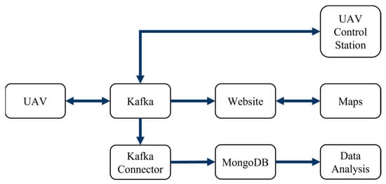
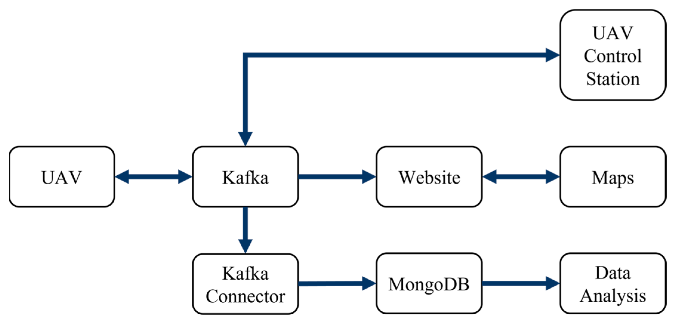
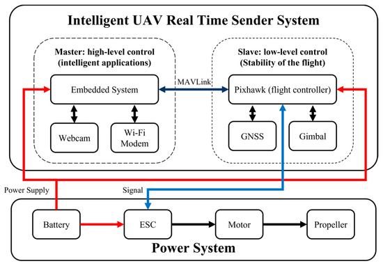
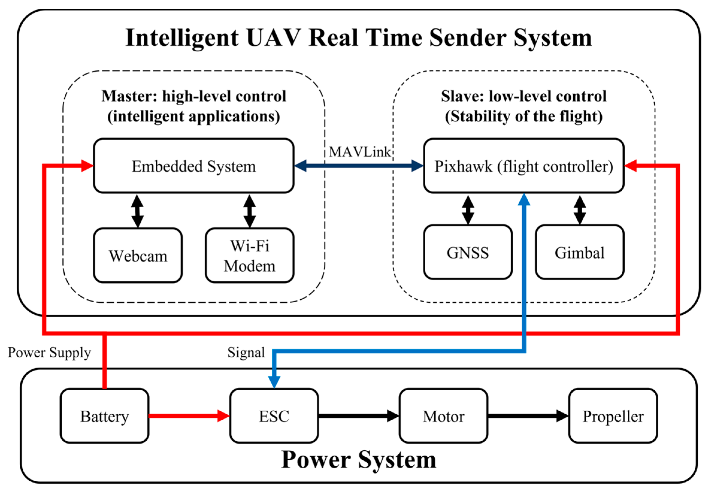
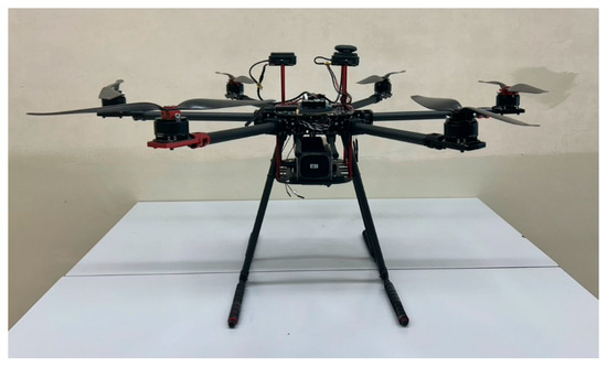
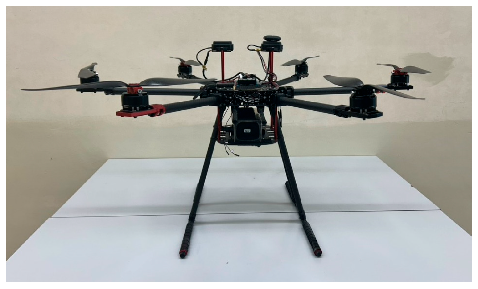
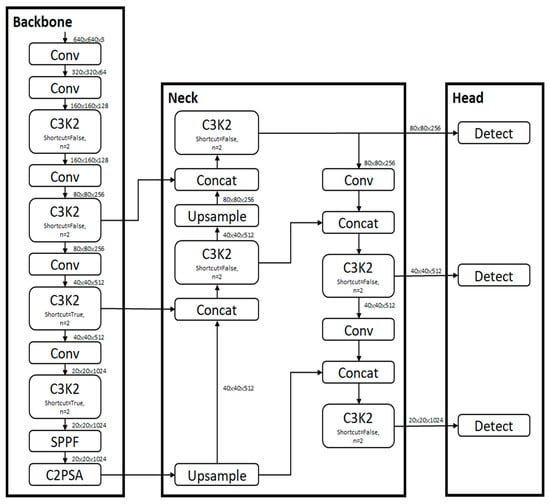
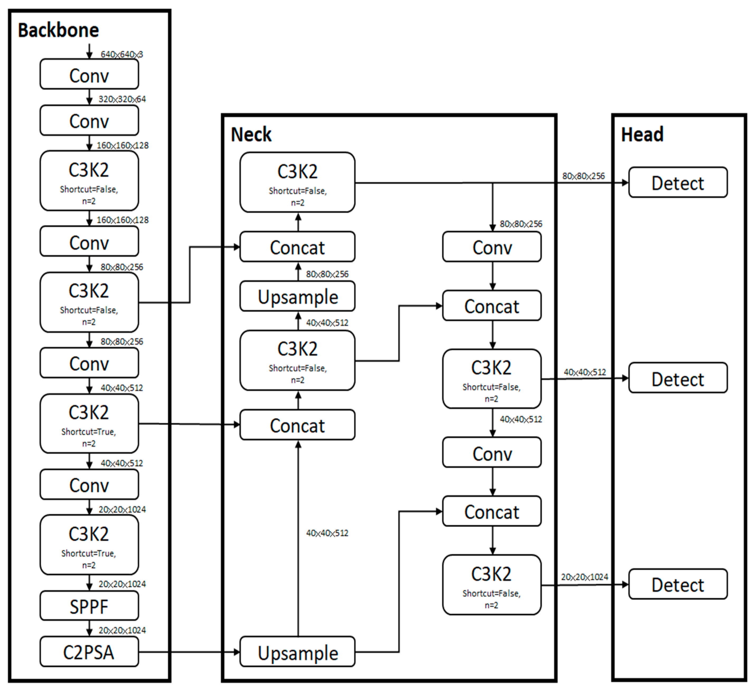
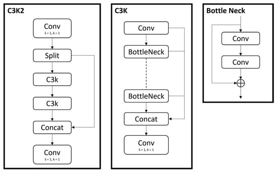
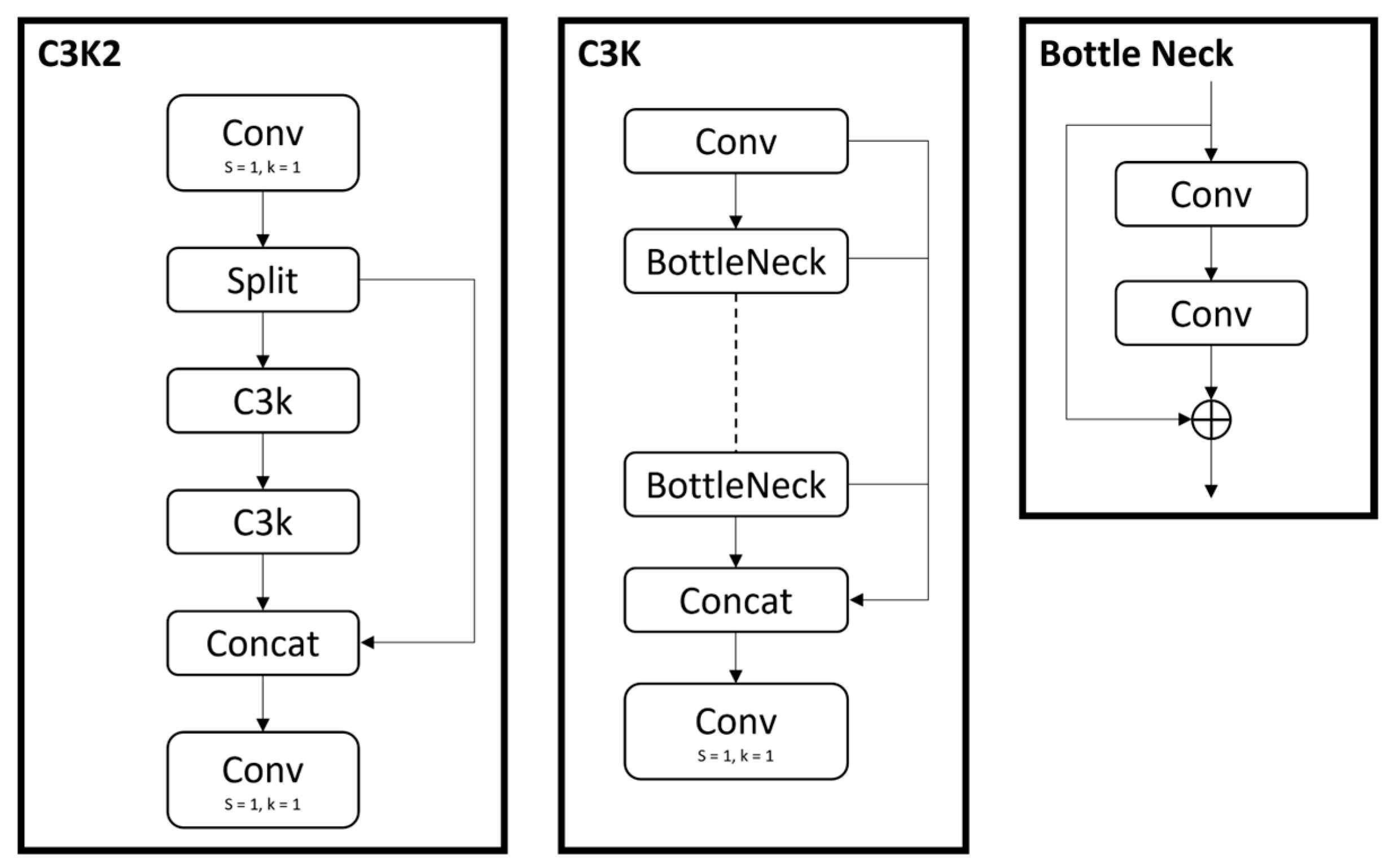
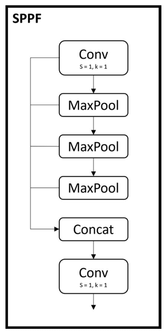
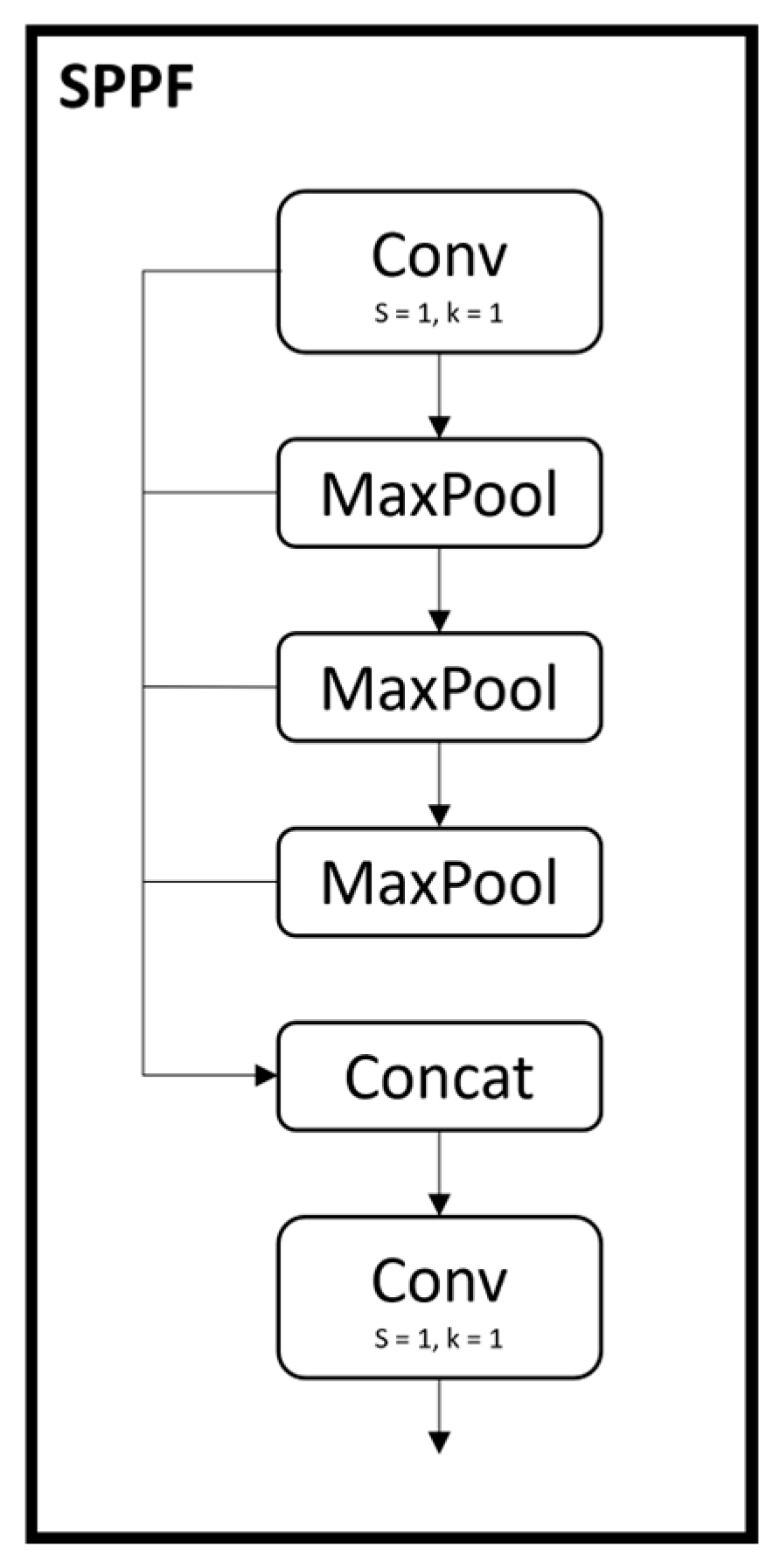
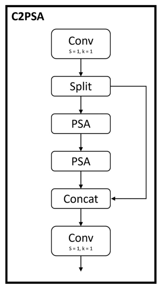
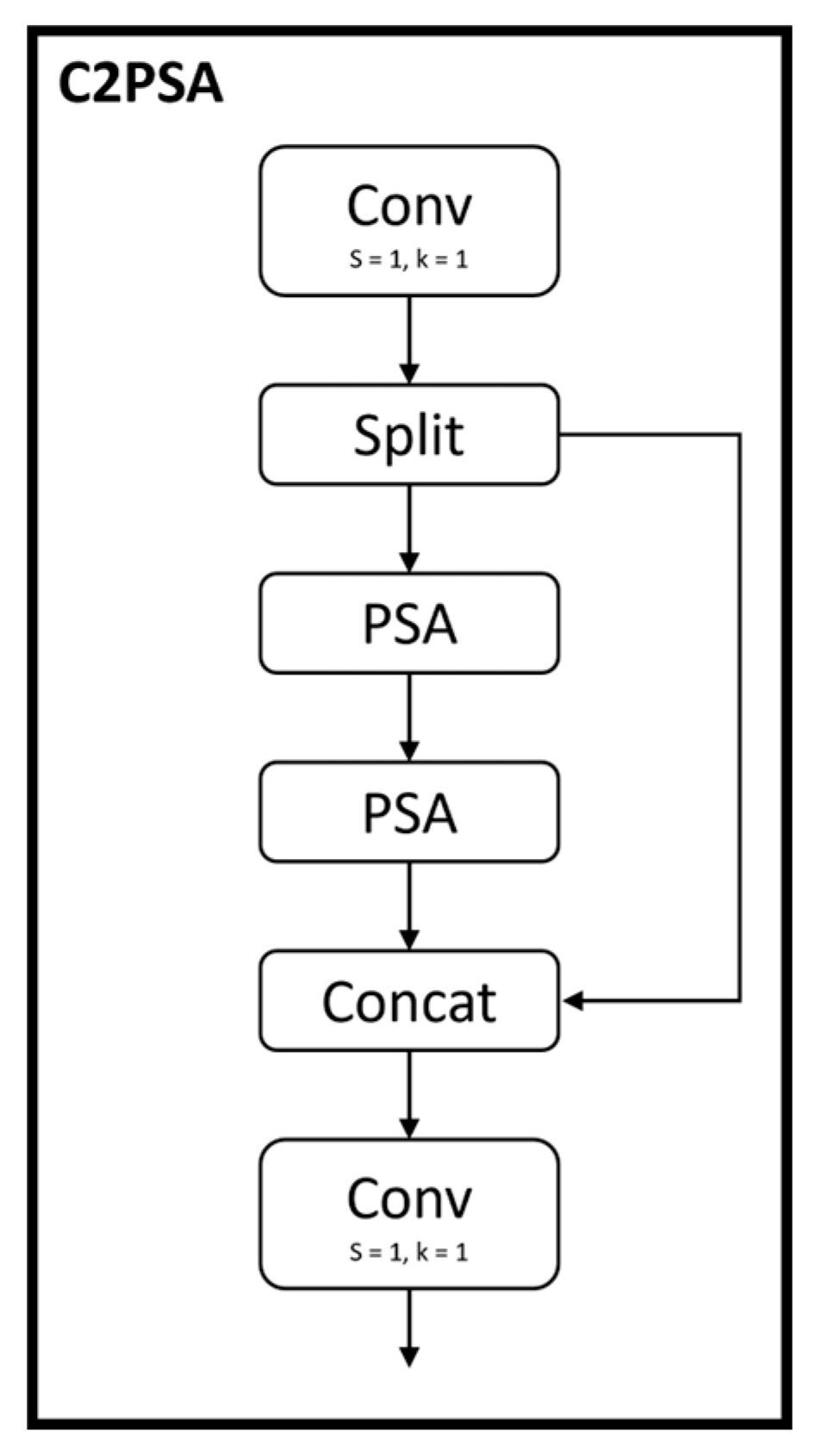
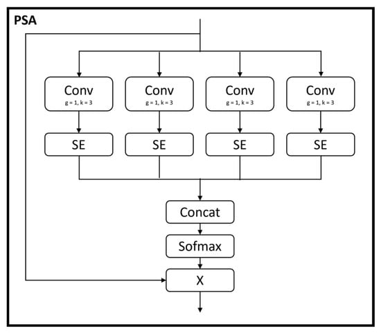
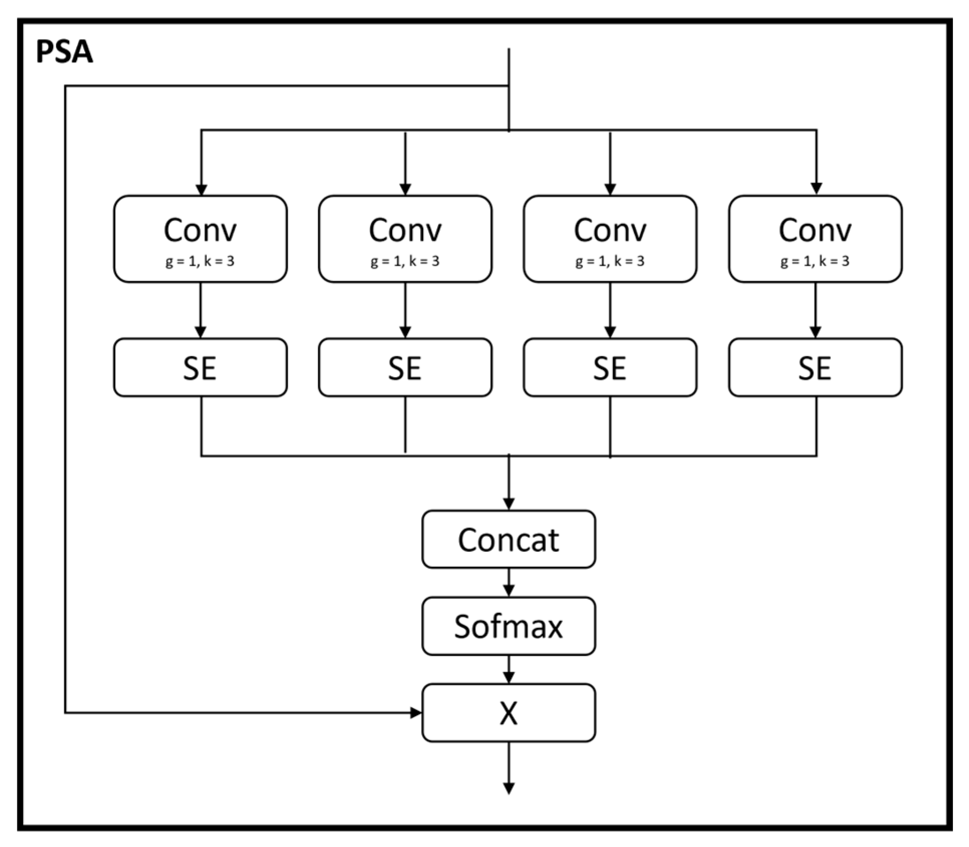
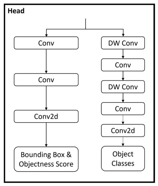
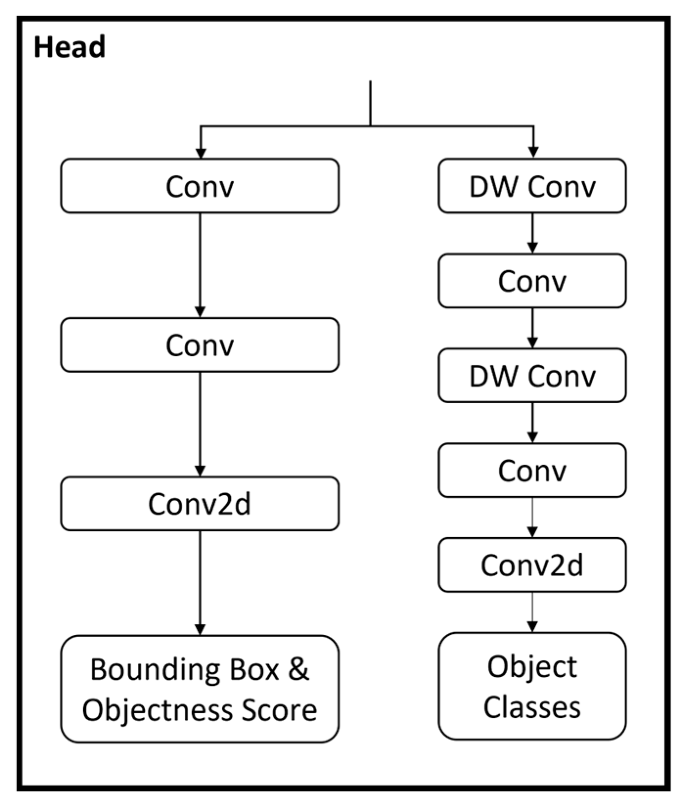
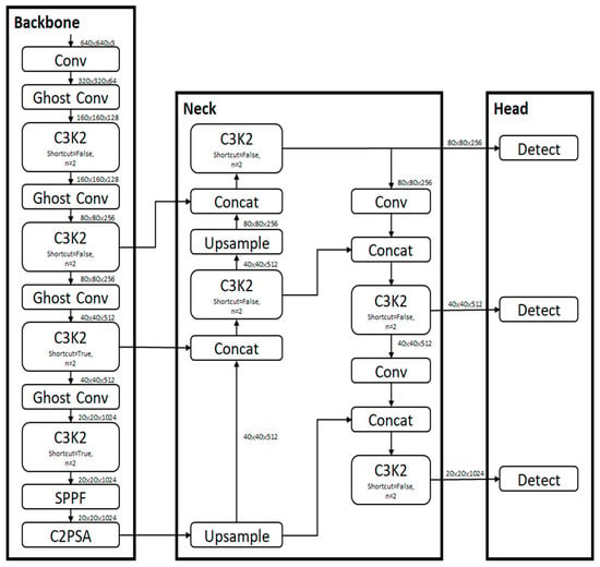
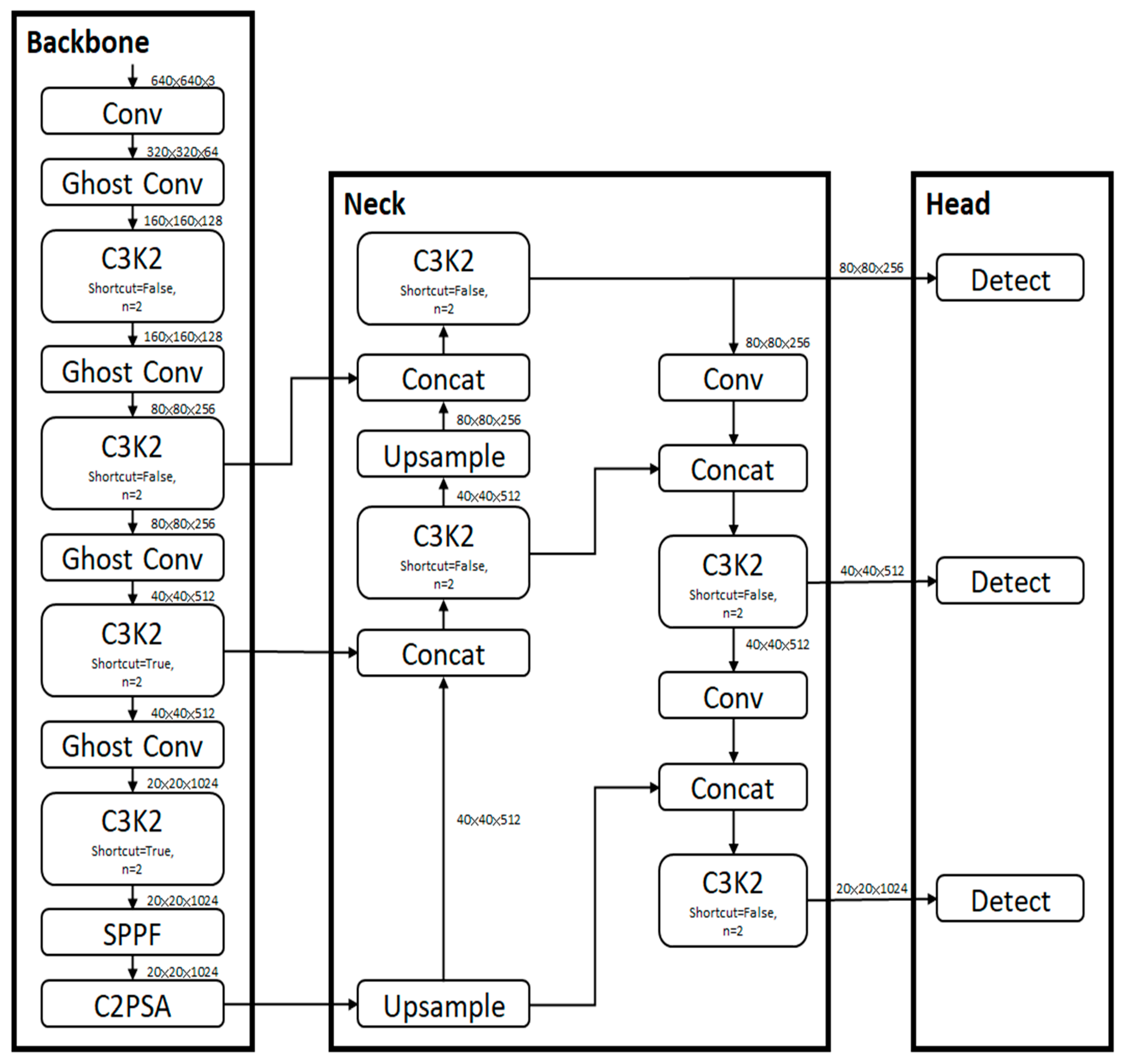
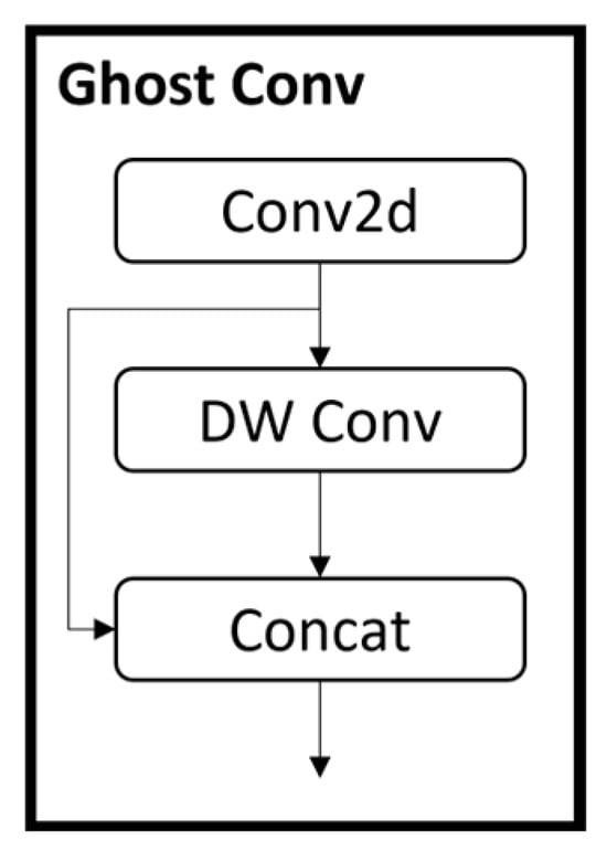
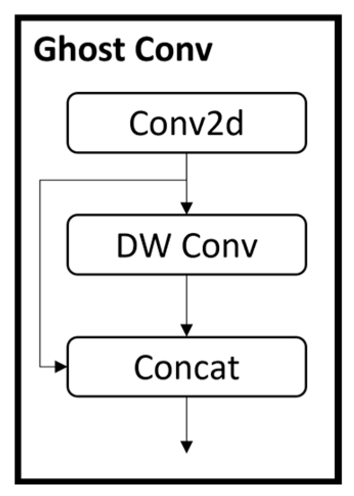
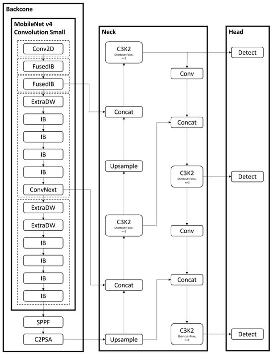
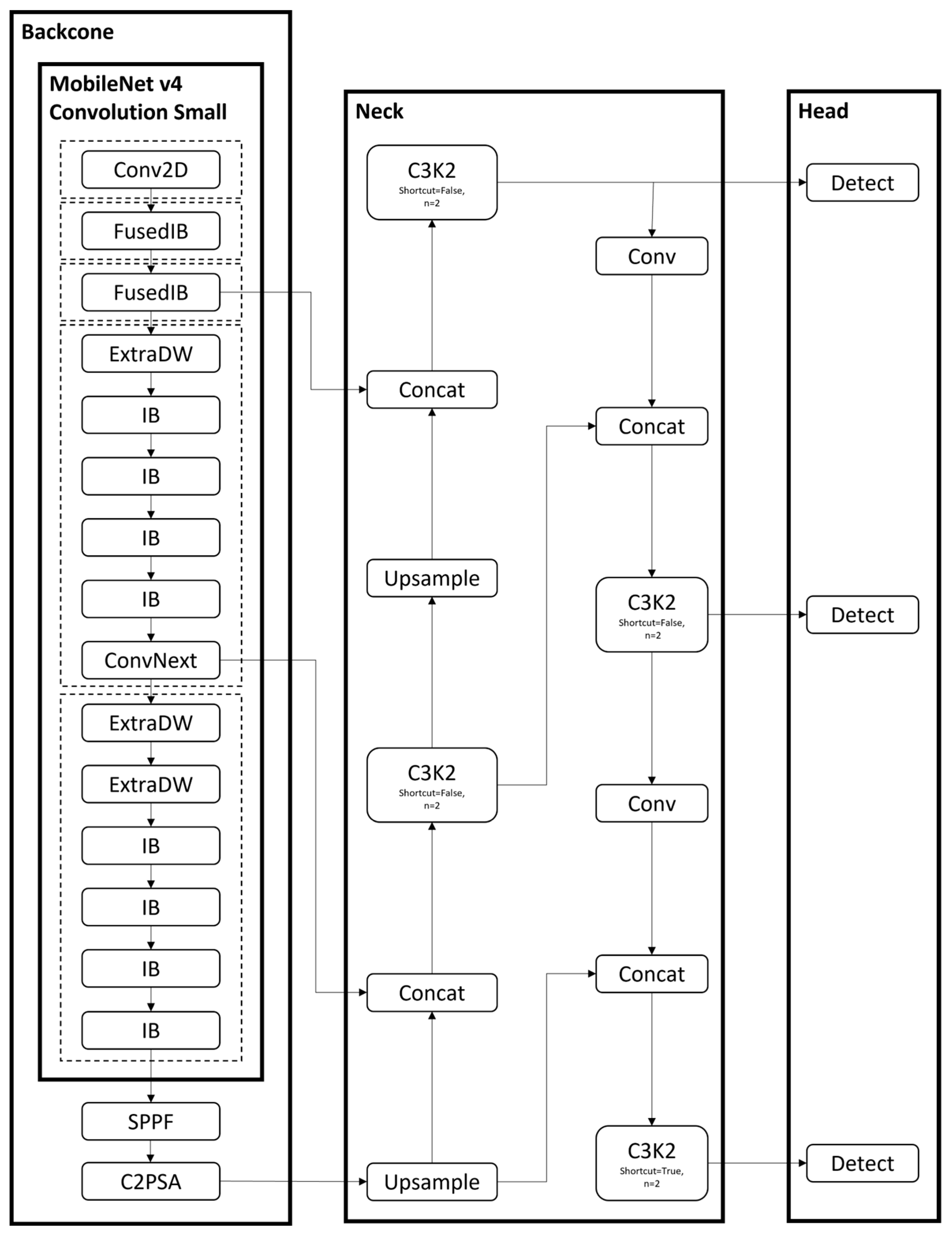
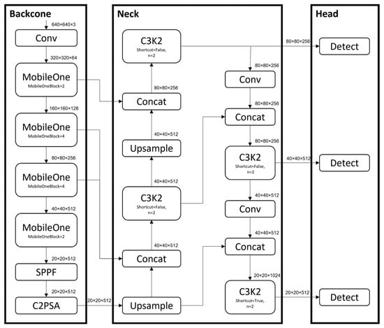
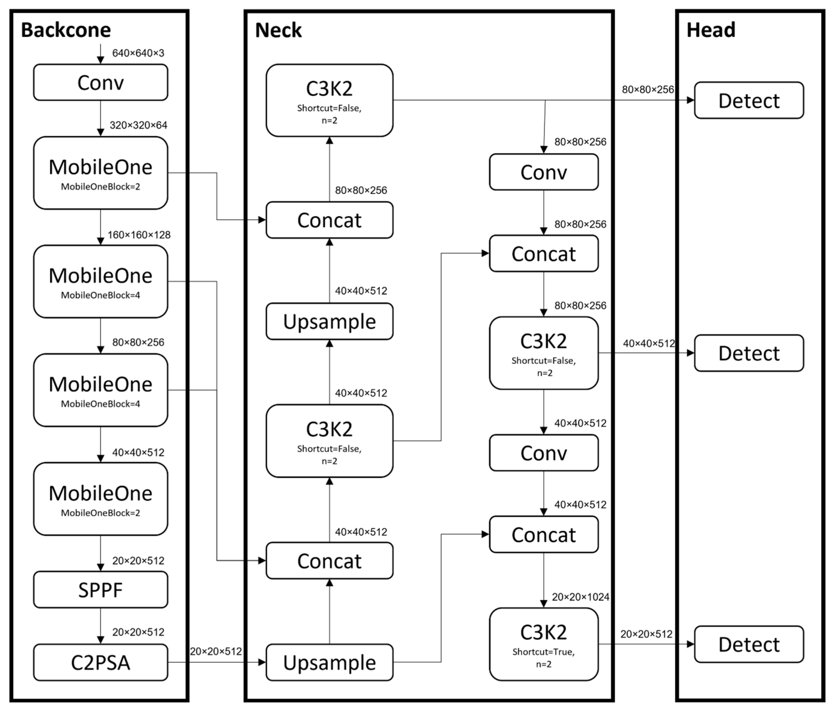
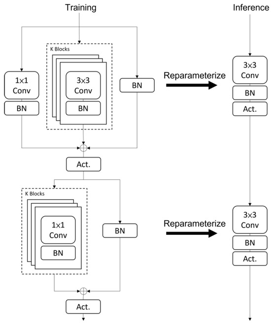
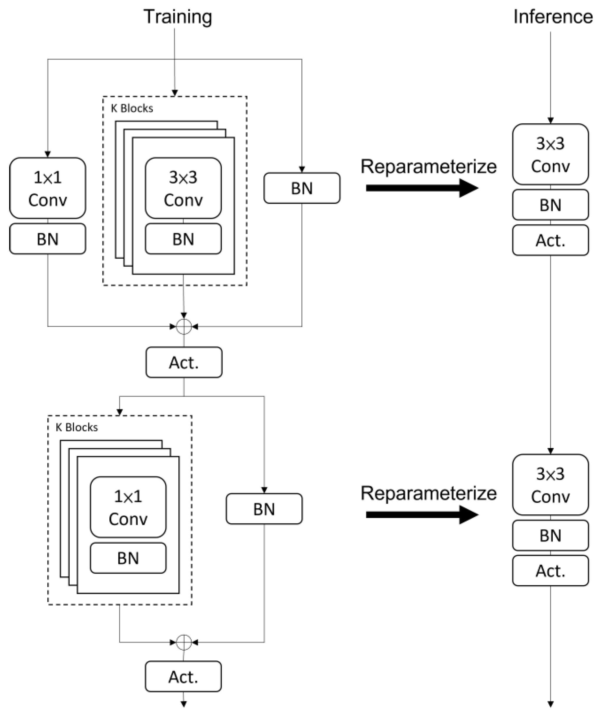
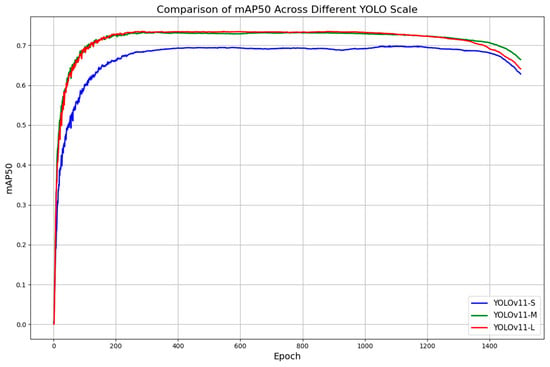
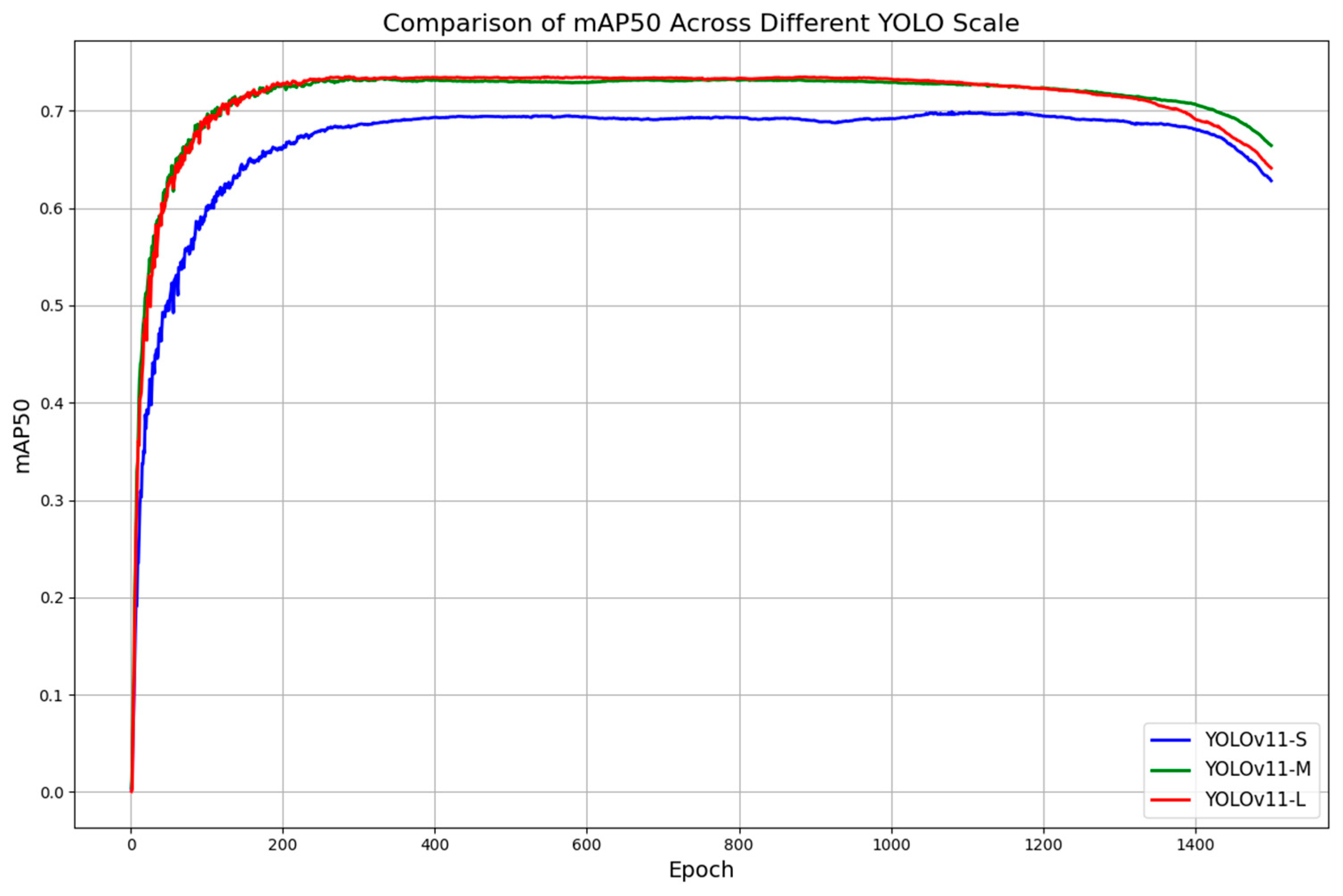
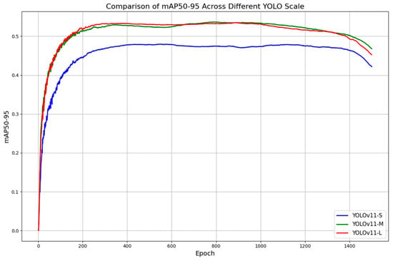
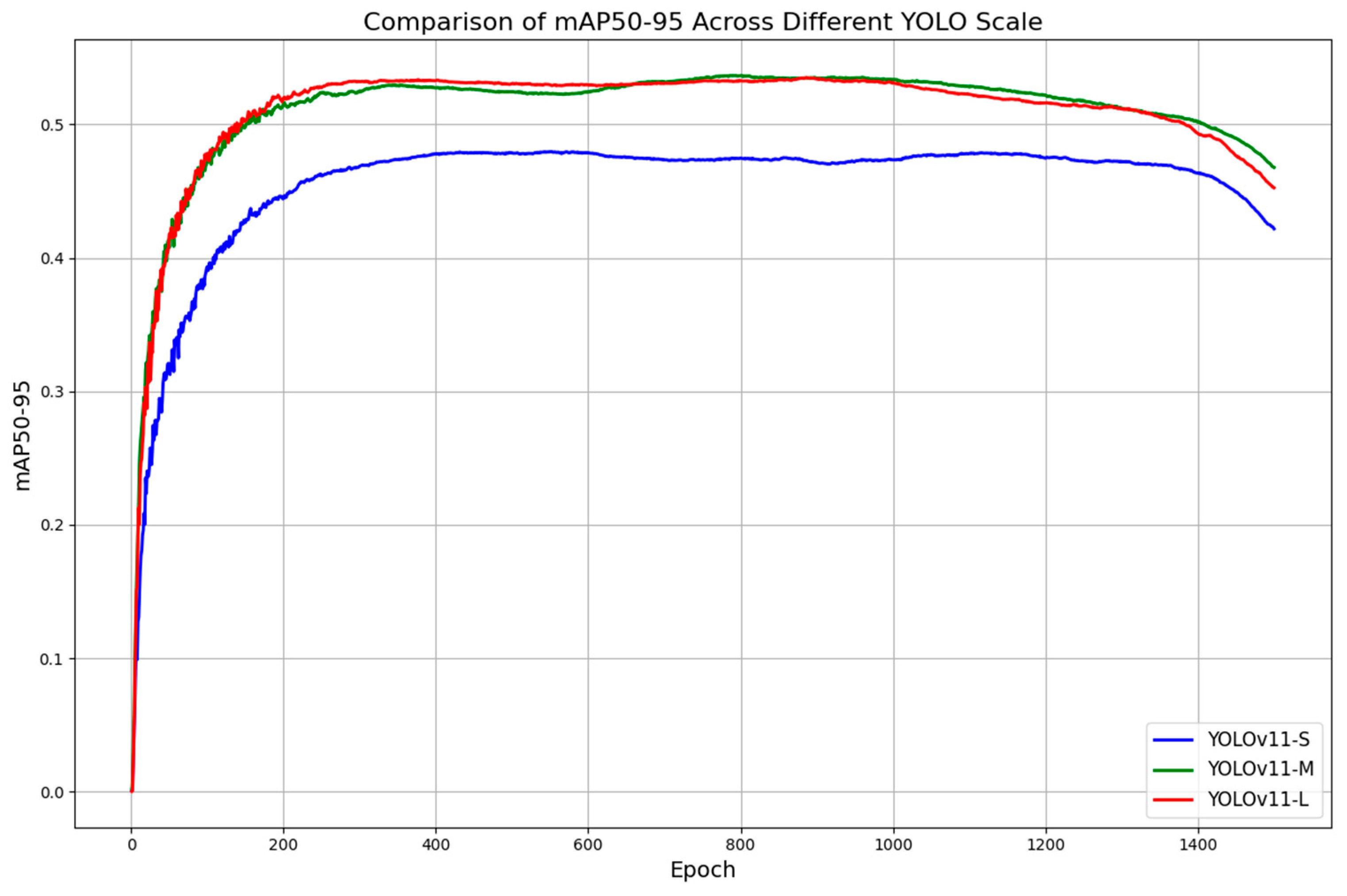
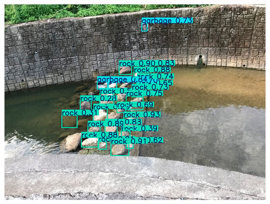
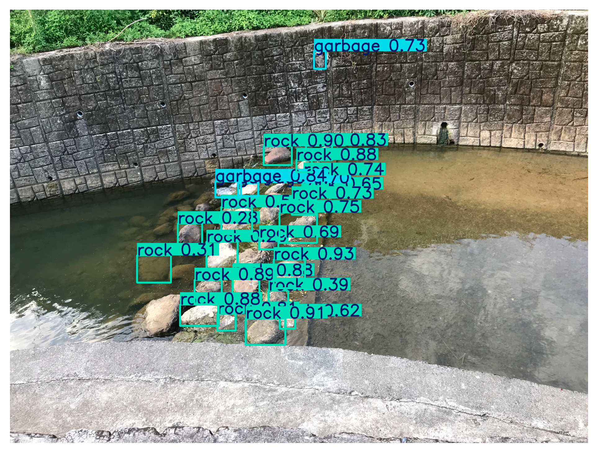
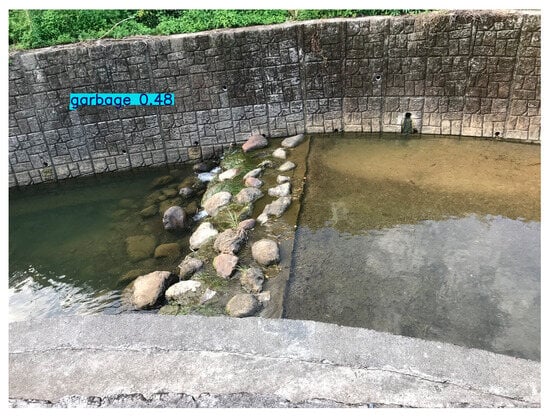
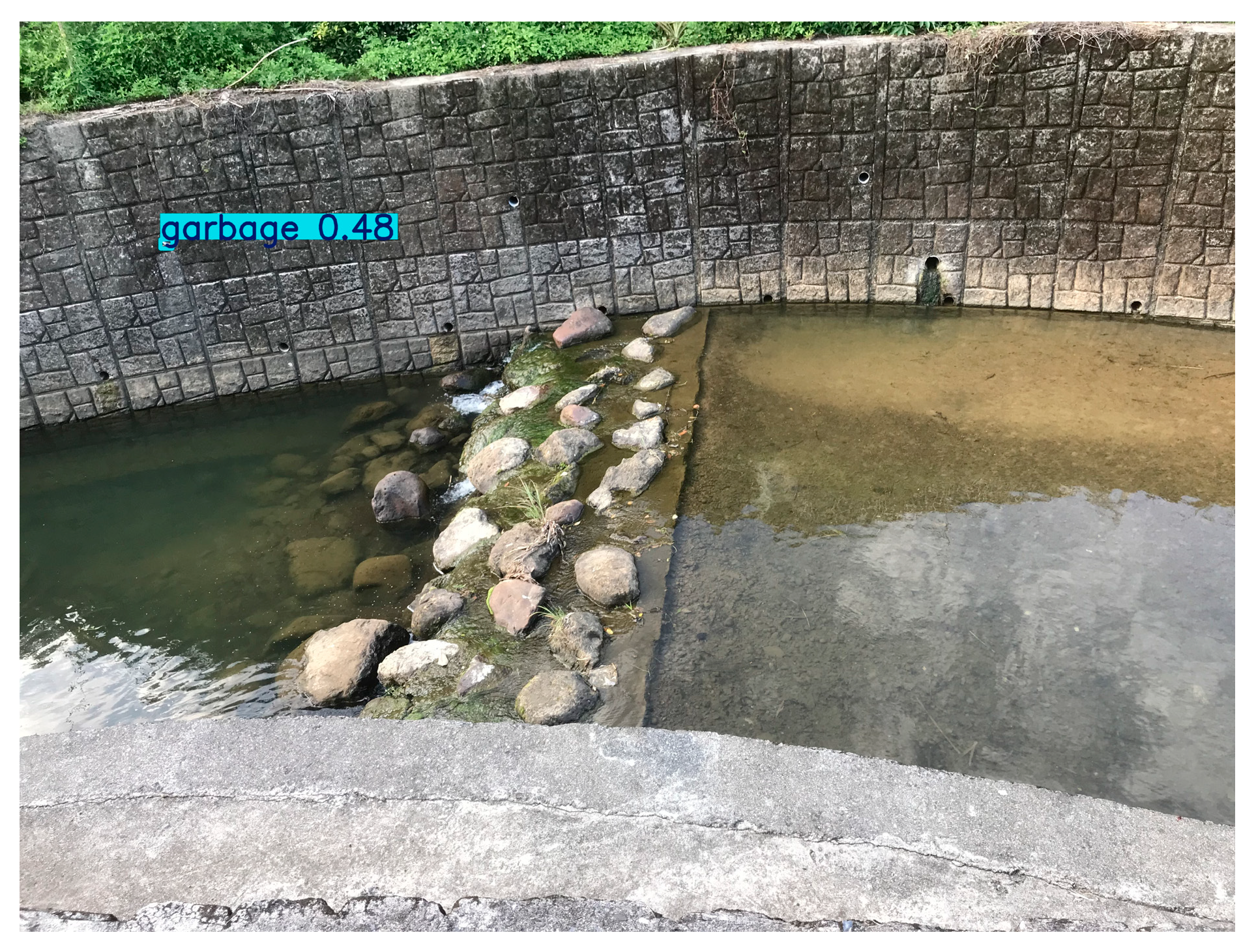
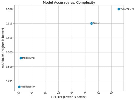
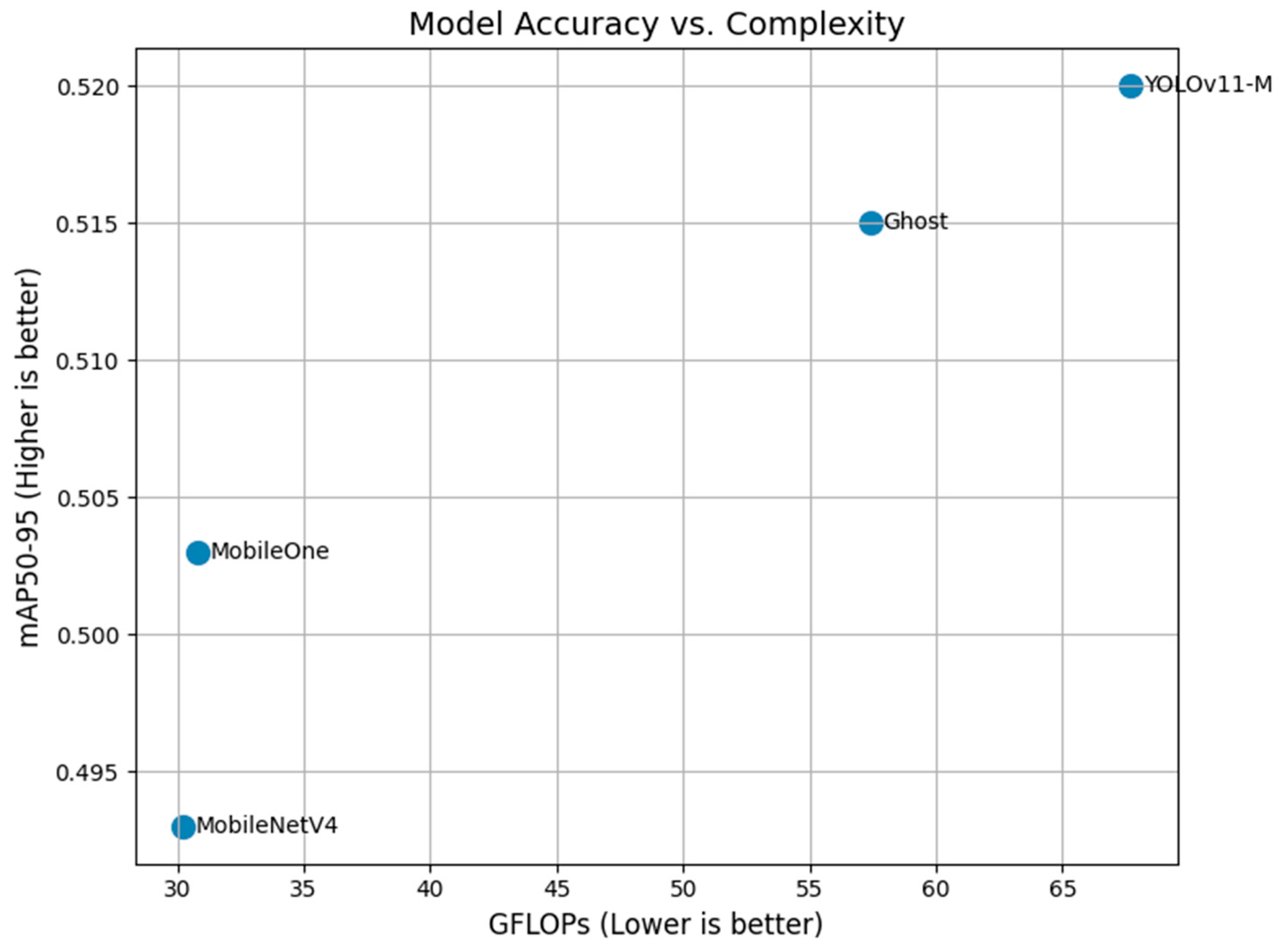
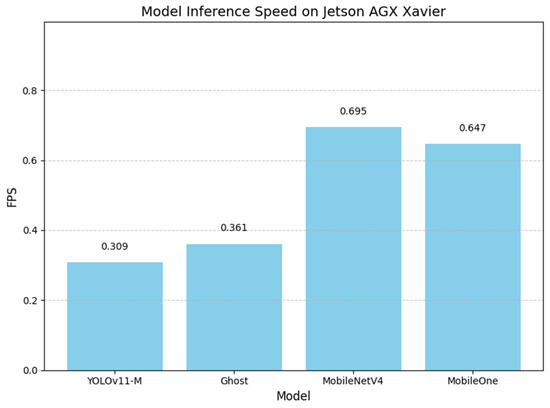
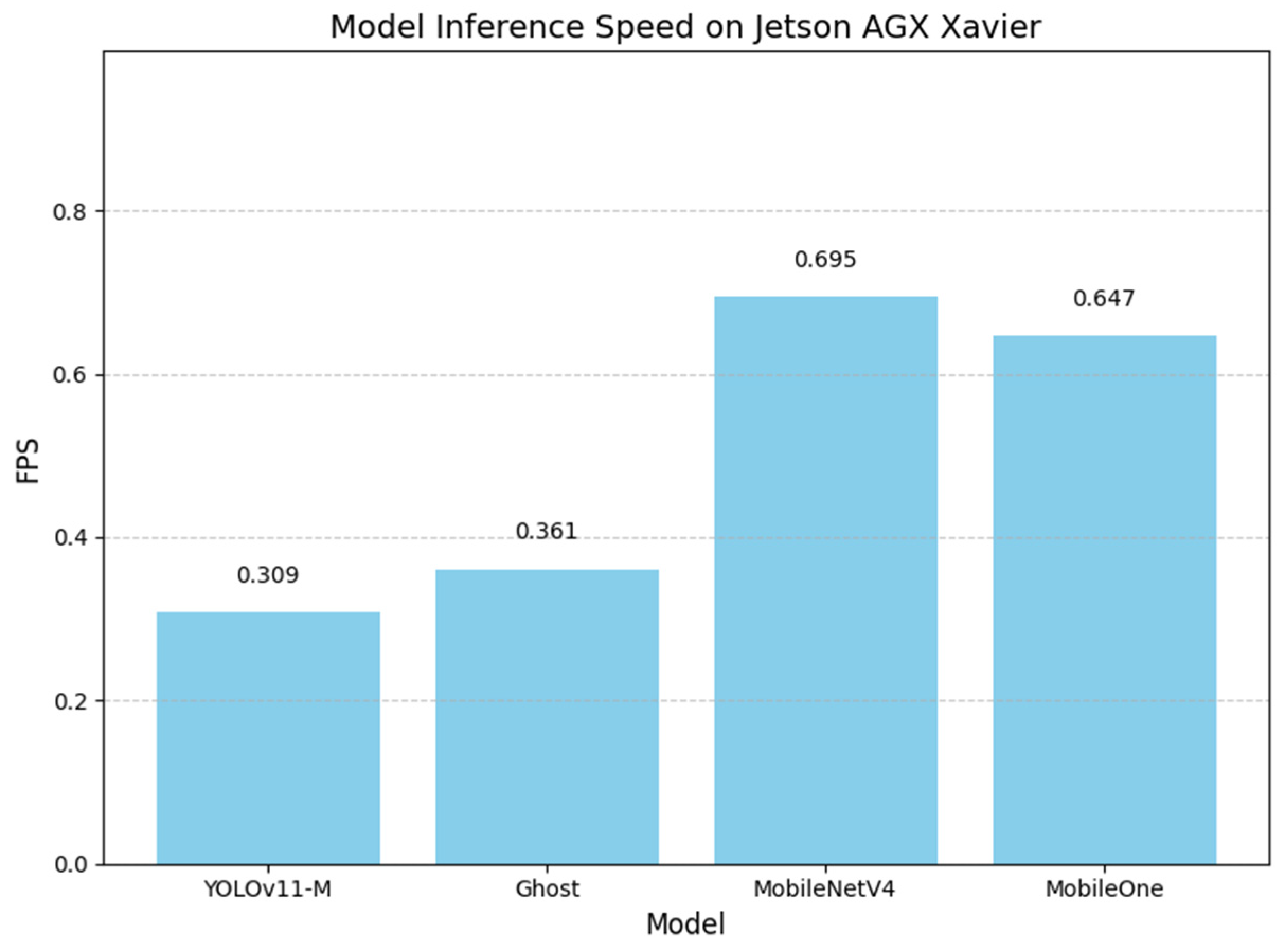
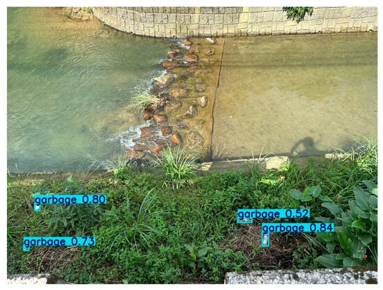
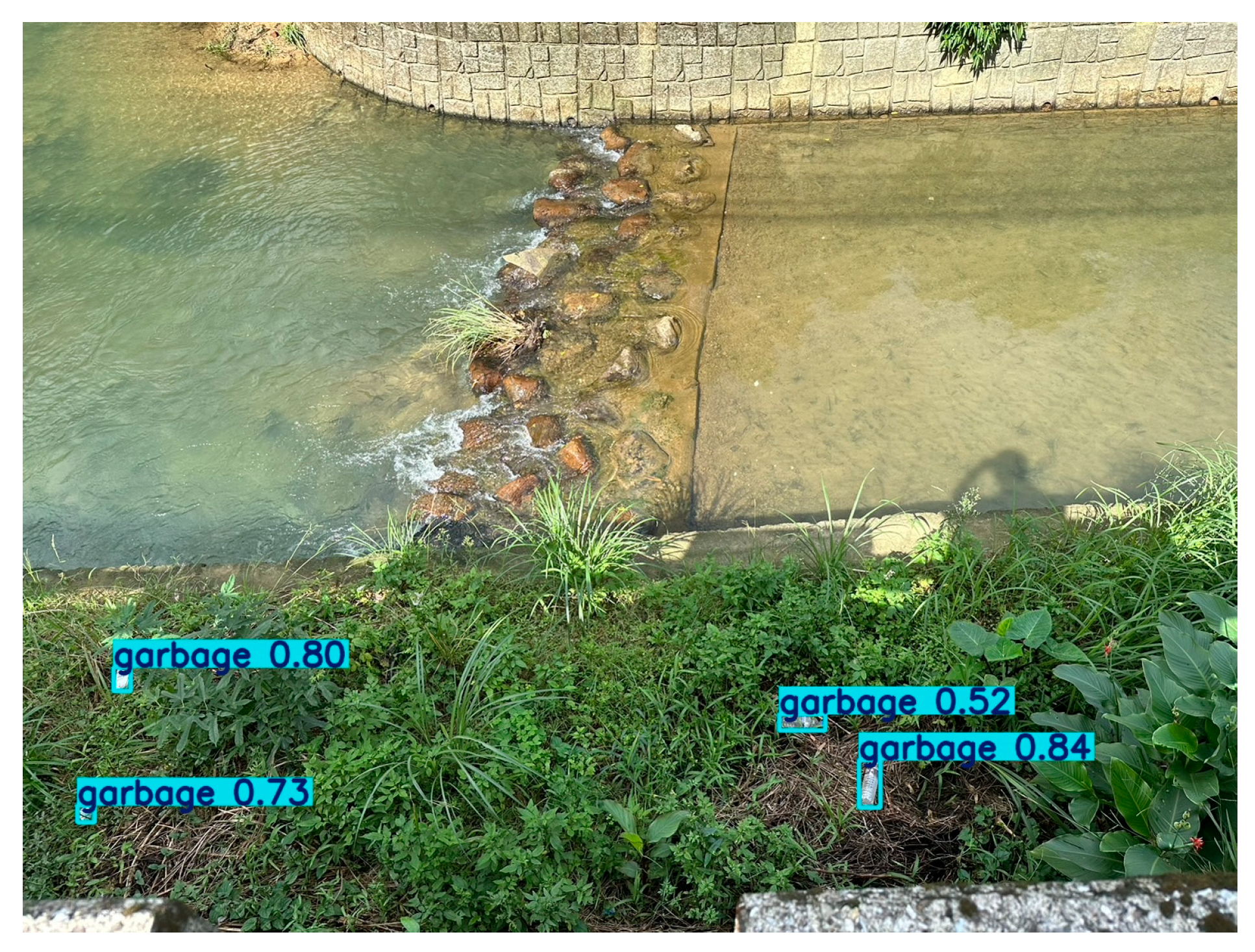
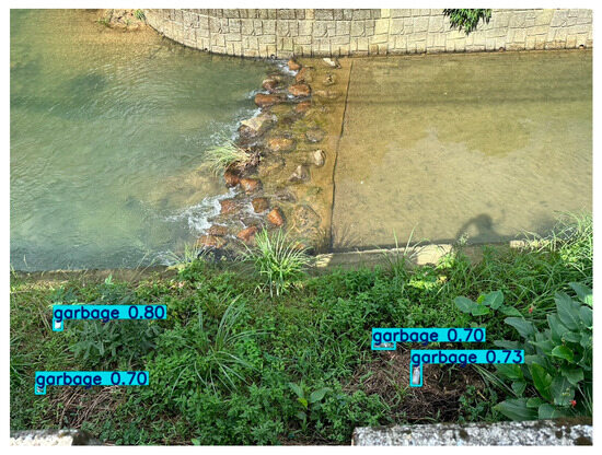
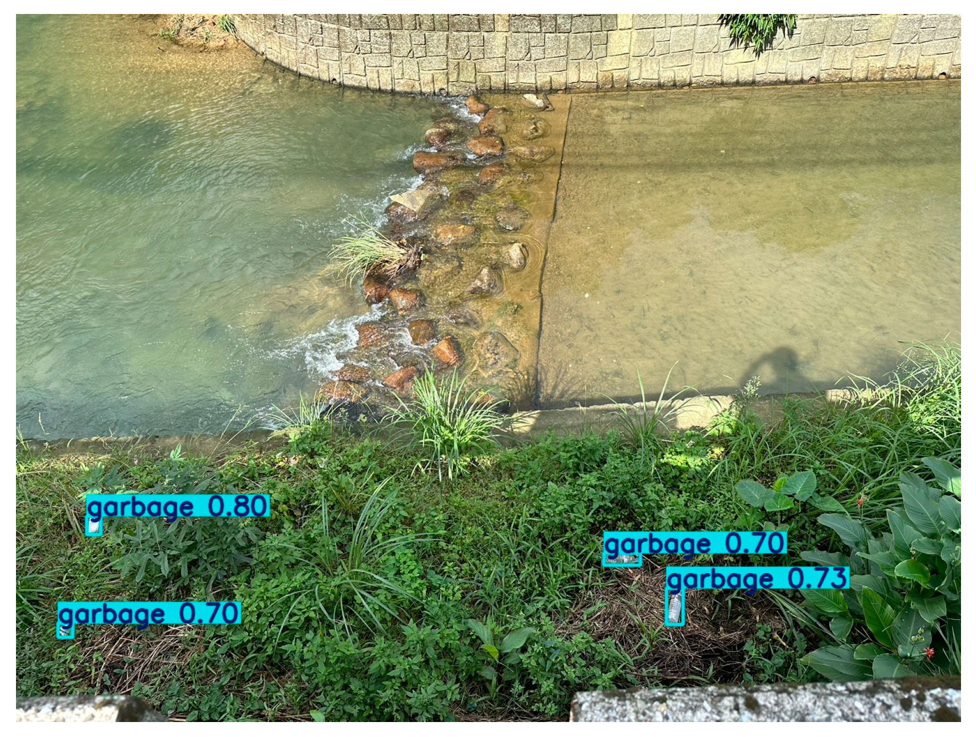
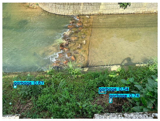
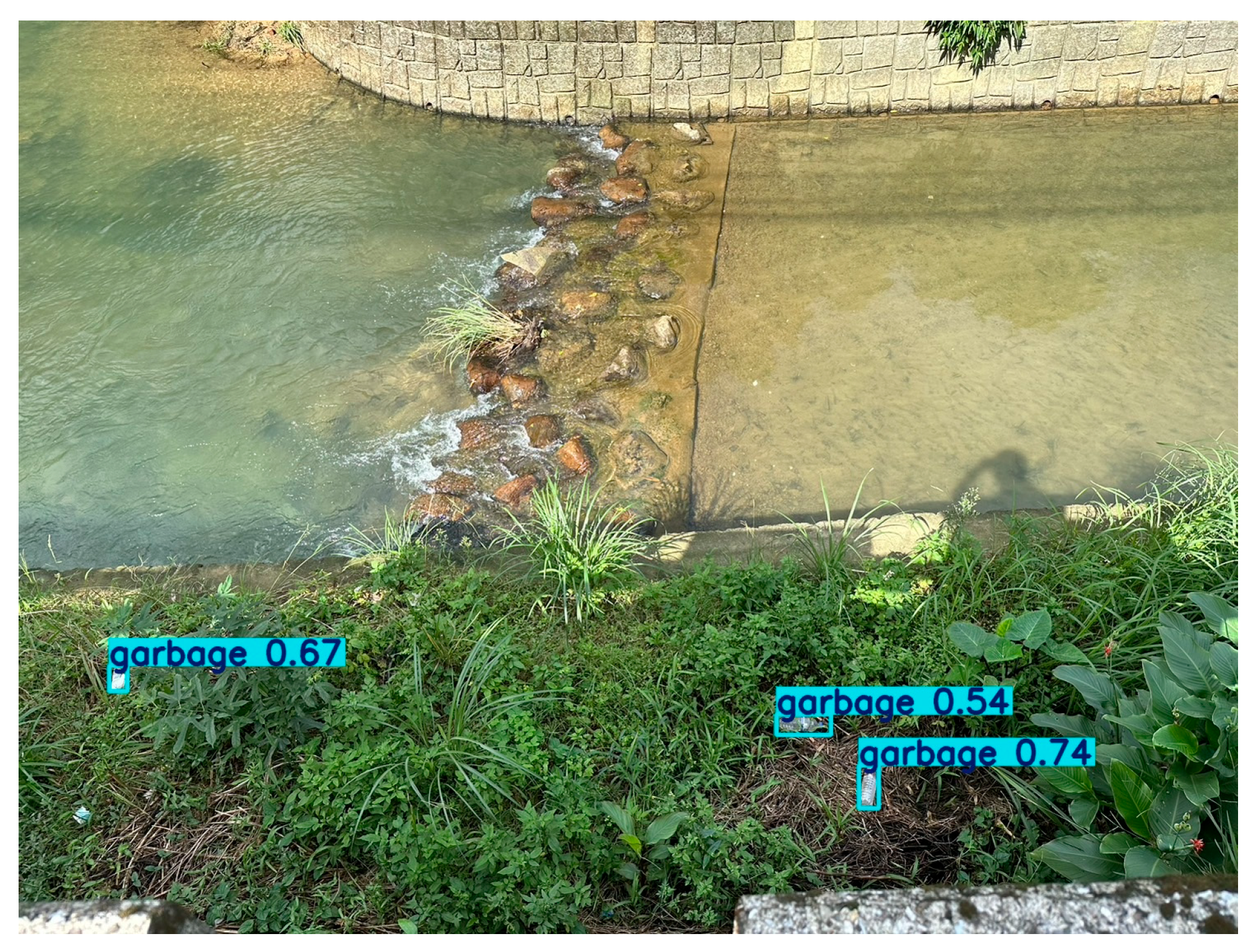
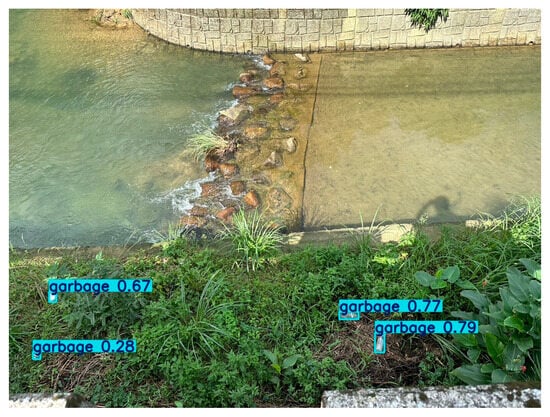
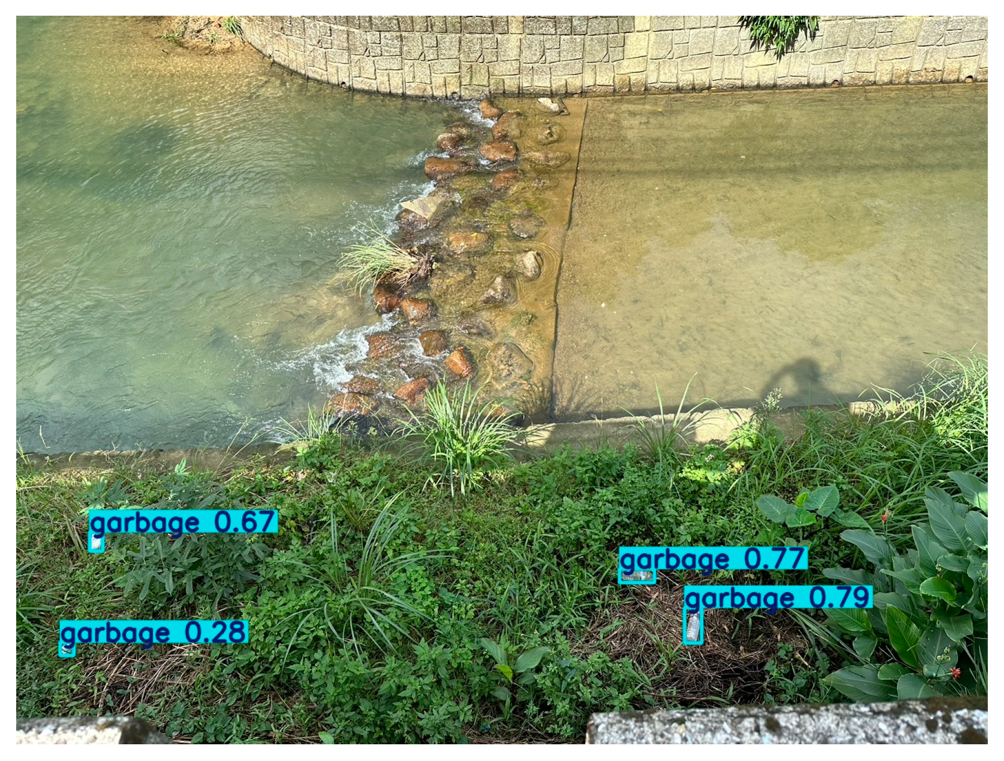
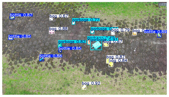
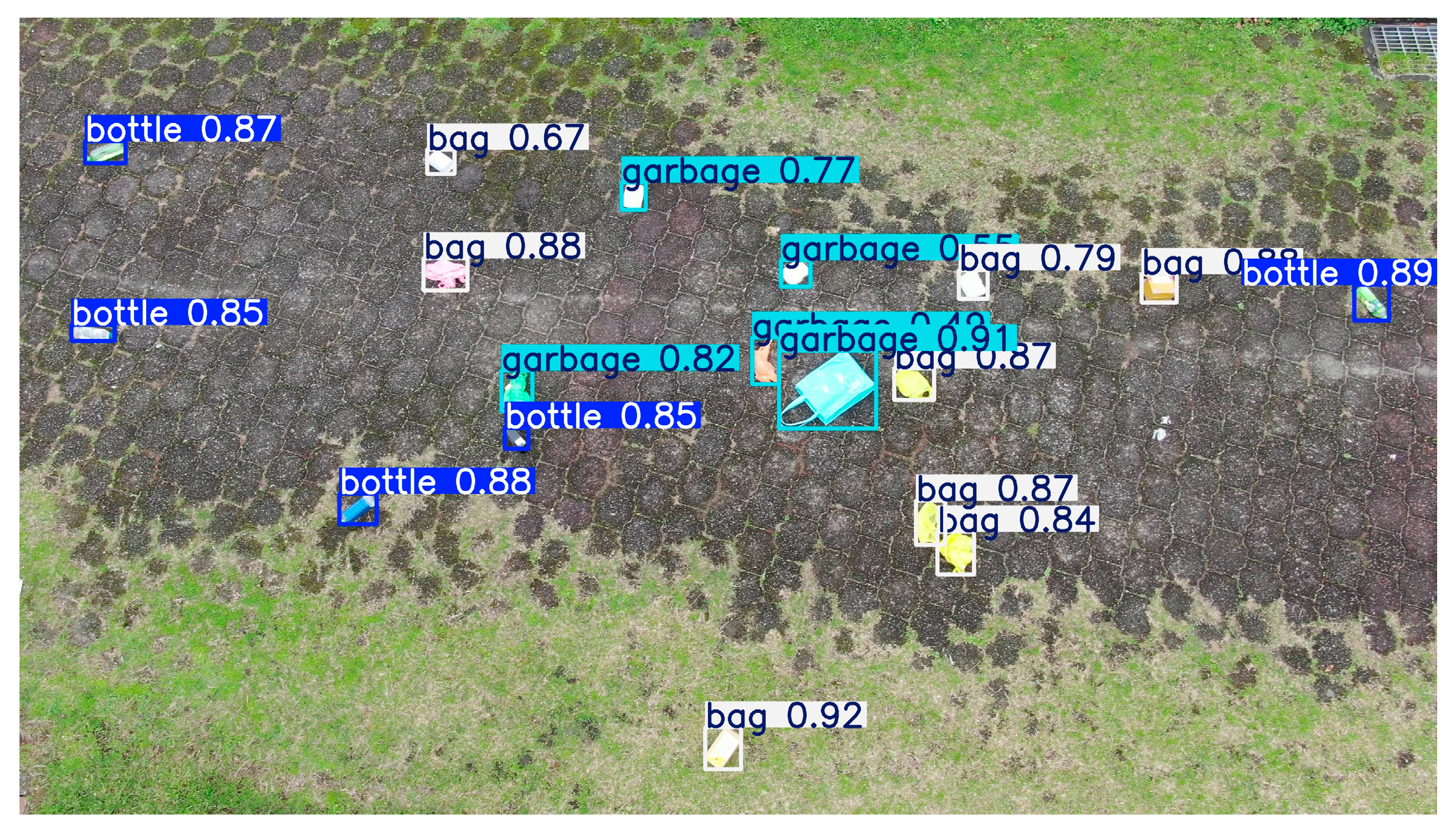
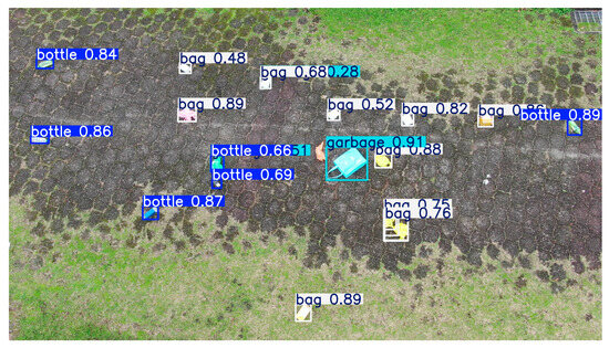
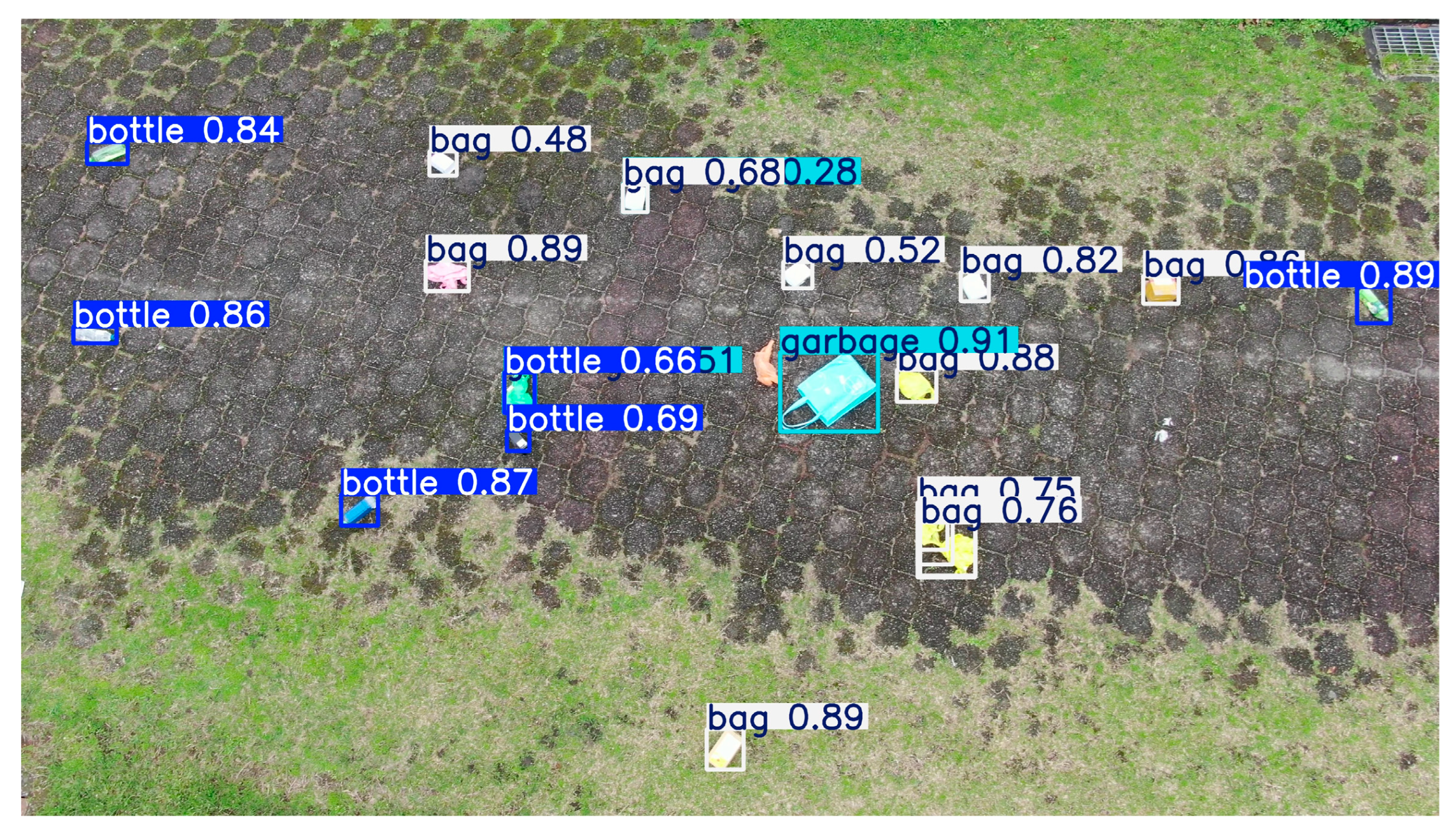
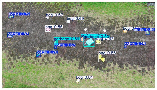
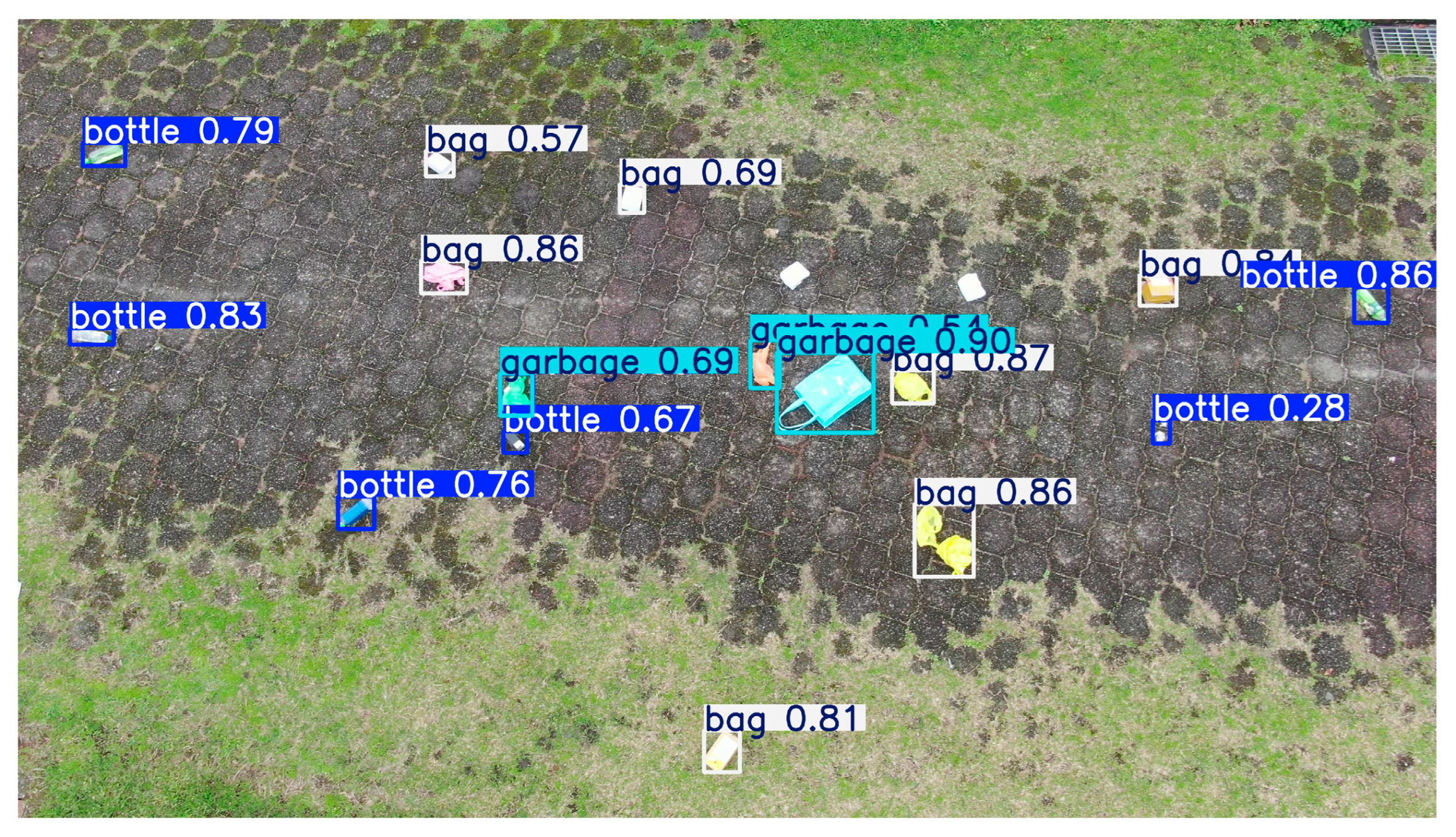
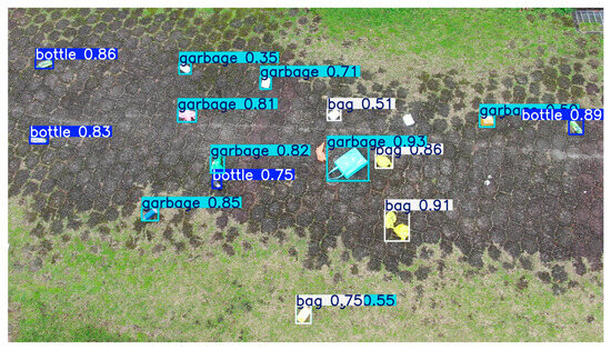
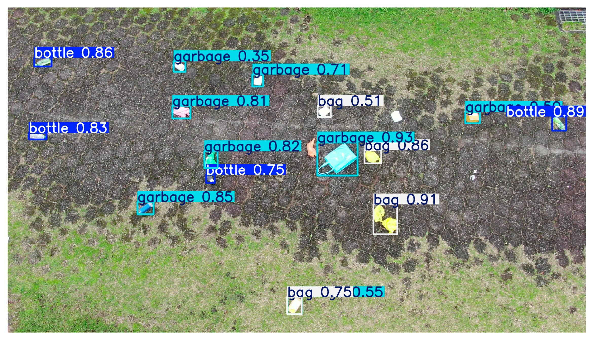

Disclaimer/Publisher’s Note: The statements, opinions and data contained in all publications are solely those of the individual author(s) and contributor(s) and not of MDPI and/or the editor(s). MDPI and/or the editor(s) disclaim responsibility for any injury to people or property resulting from any ideas, methods, instructions or products referred to in the content. |
© 2026 by the authors. Licensee MDPI, Basel, Switzerland. This article is an open access article distributed under the terms and conditions of the Creative Commons Attribution (CC BY) license.