


Abstract
The presence of silica in iron ore concentrate can have significant negative impacts on the efficiency and quality of steel production. As such, providing engineers with early and reliable information about the purity of iron ore concentrate is crucial for smooth mining operations. This paper reports on the development of a long short-term memory (LSTM) network and an ensemble data interpolation technique to enhance quality prediction in the froth flotation process of an iron ore mine. Our results demonstrate the ability of our model to accurately predict the silica content of iron ore concentrate on a minute-by-minute basis, as well as the ability to forecast hours in advance.
1. Introduction
Silica (SiO2) content is a critical quality variable in iron ore products and is routinely constrained within narrow specification windows, reflecting both downstream process constraints and market value-in-use adjustments. Industry index methodologies explicitly incorporate silica in product definitions and price normalization, e.g., high-grade products may specify silica in the low-percent range, while benchmark fines and pellets are still bounded by silica base/max ranges that are economically meaningful at the scale of 1% SiO2. In practical beneficiation operations, such constraints translate into grade-control objectives where shifts in silica can move production between value classes, motivating rapid detection and control actions when silica trends drift toward a limit [1,2].
Despite the importance of silica, continuous direct measurement can be difficult and costly in many plants, and laboratory assays introduce discontinuity and delay. A broad process-control literature on inferential sensors (soft sensors) emphasizes that real-time estimation of key quality variables is often required for advanced monitoring and control, while offline or slow analyzer measurements can degrade control performance. In mineral processing specifically, soft sensors have become a recurring theme as plants pursue tighter quality control and higher automation, and reviews of machine learning in mineral processing highlight flotation as a major application area while cautioning against overpromising without robust validation [3,4].
Flotation circuits can exhibit dynamics on minute-scale residence times, especially in intensified or pneumatic machines. Industrial residence-time studies report mean residence times on the order of a few minutes for some flotation cells (4–5 min), and the flotation literature includes cases where equivalent metallurgical performance is associated with markedly different residence-time requirements (tens of minutes in conventional circuits versus a few minutes in intensified cells). These timescales support the practical value of high-frequency estimation for advisory control and disturbance response, even when the reference assay for silica is less frequent [5].
In recent years, the mining industry has undergone significant modernization in many areas through the integration of advanced technologies such as machine learning (ML) methods. Deep learning (DL) models, such as long short-term memory (LSTM) networks, have shown promising results in various industries because of their ability to process large datasets, reveal patterns, and make accurate predictions.
This study presents a DL-based framework that pairs an LSTM network with an ensemble data interpolation technique for quality prediction in the froth flotation process of an iron ore mine. The framework enables real-time monitoring of silica content in the concentrate and forecasting of future levels. By providing engineers with this valuable information, the proposed solution aims to enhance the decision-making processes, leading to more efficient, sustainable, and environmentally friendly steel production.
2. Literature Review
In the context of ironmaking, iron is produced from iron ore using reducing agents in a blast furnace. Studies have shown that the presence of trace elements like silica in iron ore concentrate leads to higher consumption of reducing agents [6], meaning that ores with higher silica content are less efficiently processed for steel production and increase the overall production cost due to the higher energy consumption. This understanding was furthered in another study that found that reducing the silica content of the ore is beneficial for increasing the capacity utilization of blast furnaces, thereby decreasing fuel consumption and increasing output [7].
The challenges posed by high silica contents in ore concentrate extend beyond poor energy efficiency. One study showed how the presence of silica can enhance the formation of potentially harmful spinel inclusions in steel, which occurs through the reduction of magnesium and calcium oxide in slag [8]. Another study further highlighted this issue through a discussion of the detrimental effects of silica-rich oxide inclusions in stainless steel, such as reduced impact toughness and the promotion of stress corrosion cracking [9].
High silica content, especially when combined with increased austenitizing temperatures, leads to a significant increase in core hardness [10]. However, this is accompanied by a marked decrease in fracture toughness and wear resistance. Conversely, for steel with low silica contents, an increase in core hardness does not sacrifice but rather enhances fracture toughness and significantly improves wear resistance. In a related study, a linkage was established between the composition of concrete and its structural integrity, finding a decrease in compressive strength with an increase in steel slag content, which often contains varying levels of silica [11].
The environmental repercussions of mining and processing activities that produce materials with high silica contents are also noteworthy. One study identifies the environmental hazards posed by tailings, which are often contaminated with silica or other impurities. These tailings are typically stored as slurries in ponds confined behind dams or impoundments, with around 3500 active tailings impoundments reported globally in 2000 [12].
A promising avenue for addressing the operational and environmental challenges posed by mining operations lies in adopting digital technologies, particularly ML approaches. Several studies highlight the potential of ML in optimizing mining operations, from truck dispatch systems to the selection of mining equipment and process flowsheets, enhancing productivity and safety [13,14,15]. The use of ML models, particularly support vector machines and deep learning models, has been gaining traction since 2018, with applications ranging from mineral exploration to the automation of decision support systems [16,17].
Several studies emphasize the transformative impact of integrating neural networks and reinforcement learning in mining operations, marking a significant leap toward achieving operational autonomy with intelligence [18,19]. Another study further advocated for the application of ML in extracting and analyzing extensive mineralogical data, a critical need given the global demand for raw materials and the complexities of ore deposits [20]. Another study focused on predicting impurity levels in ore concentrate, facilitating corrective actions [21].
3. Materials and Methods
3.1. Dataset Information
This research employs a dataset of information collected over the span of seven months, from March to September, during the froth flotation phase of a mining process [22]. This data includes quality metrics of iron ore pulp prior to being fed into the flotation plant, variables that impact the final quality of ore, process data including the level and airflow inside the flotation columns, and the final measurements of quality upon completion of the flotation process. In total, the dataset consists of 737,454 data points across 24 features. These features are detailed in Table 1.
Table 1.
Feature information.
3.2. Data Preprocessing
Preprocessing is an important step in any ML process as it can help prevent any issues that may be present in the data prior to the application of a ML model. The mining data used in this research underwent several phases of preprocessing prior to work beginning on the LSTM model. The various stages of preprocessing are outlined below.
The first issue that was addressed dealt with the timestamps of the data collected. The first set of data was collected from March 10 to March 16, but there existed a gap between this first set of data and the rest of the collected data, which spanned from March 29 to September 9. Gaps in time series data can negatively impact data analysis and can lead to incorrect results [23] so this gap needs to be addressed before the LSTM model can be applied. To correct this issue, the 26,814 data points between March 10 and March 16 were removed from the dataset, so March 29 became the new starting point of the dataset, which then consisted of 710,640 data points.
The second issue to be corrected was a syntaxial one, where the data set used commas instead of periods to indicate decimal numbers. To properly process the data, the values needed to be read numerically so, to fix this issue, the commas were simply replaced with periods. Another important issue lay in how the data was collected. In the original dataset, the data for the quality measurements of the iron ore, both prior to and after the froth flotation process, were collected on an hourly basis, while all the data for the environmental and process variables were collected every twenty seconds. This led to the values in the columns representing the raw and processed materials being repeated every twenty seconds until the hour changed, a cycle that continued until the end of the data collection process. To fix this issue, the entire dataset was down sampled to only include the first set of values from every hour, taking the total number of data points in the dataset from 710,640 to 3948.
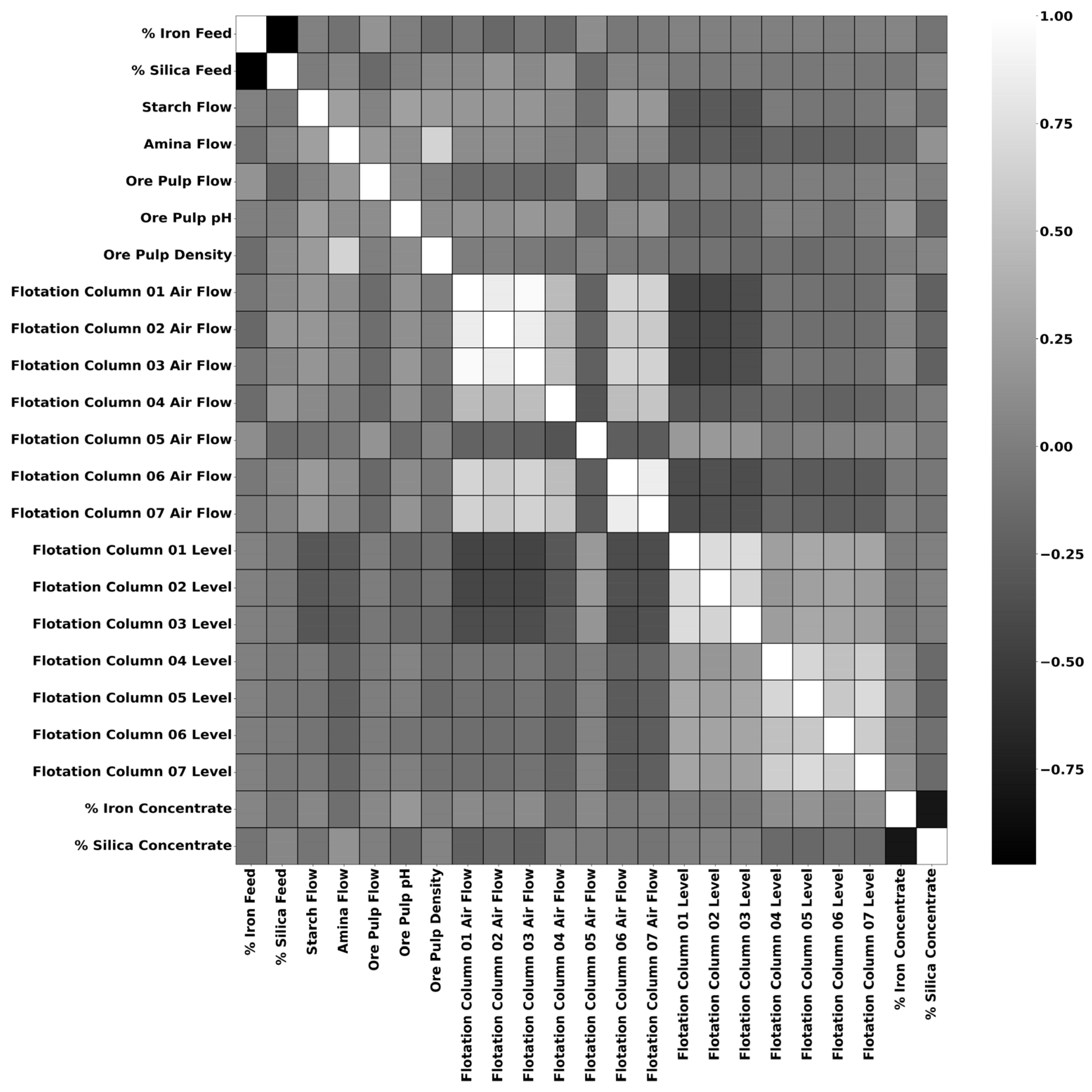
The next stage of preprocessing was feature selection, which is a method of selecting relevant features in a way that results in simpler and more comprehensible models [24]. There are many different methods for performing feature selection, including correlation-based methods, which is the approach employed in this research. Correlation-based feature selection is based on the central hypothesis that a good feature set contains features that are highly correlated with the class but not each other [25]. A correlation matrix showing the correlations between the features of the mining dataset is shown in Figure 1.
Figure 1.
Correlation matrix for the features of the dataset.
From the correlation matrix, it is apparent that the ‘% Iron Concentrate’ and ‘% Silica Concentrate’ features are highly correlated. To prevent issues related to redundancy, overfitting, and interpretability, one of these features need to be removed from the dataset. Since the objective of this research is to determine the amount of silica in iron ore concentrate, the ‘% Iron Concentrate’ feature was selected for removal.
As a final note in this section, we would like to highlight how our preprocessing and LSTM followed by ensemble data interpolation methodology improves upon existing methods of iron ore concentrate modeling. While silica measurements in our dataset are collected hourly, the flotation process itself is continuous and influenced by process variables (e.g., airflow, reagent dosage, pulp density, and column levels) that are recorded at much higher frequencies (every 20 s). These variables can induce changes in separation performance on much shorter time scales than the measurement interval.
In practice, operators must make timely adjustments to maintain product quality and recovery. Relying solely on hourly laboratory measurements introduces a delay that can limit the effectiveness of control actions. The goal of our approach is therefore not to replace laboratory measurements, but to provide higher-resolution estimates of silica content between sampling intervals. The interpolation step allows us to align the prediction output with the time scale of process dynamics, enabling near real-time monitoring and more responsive decision-making.
3.3. LSTM Network
An artificial neural network (ANN) is a powerful ML model that is inspired by the human brain, consisting of layers of interconnected nodes or “neurons”. ANNs process information by transmitting signals through these nodes, each weighted and adjusted during learning phases to improve accuracy. The layers of an ANN include an input layer that receives data, hidden layers for processing, and an output layer that delivers the result. ANNs are widely used in various applications, from image and speech recognition to natural language processing and predictive analytics, due to their flexibility and capability in handling diverse and complex tasks. There are many variations of ANNs, but they can be largely classified into two broad categories: feedforward neural networks (FNNs) and recurrent neural networks (RNNs).
FNNs are characterized by a unidirectional data flow, where information moves linearly from the input layer through hidden layers and finally to the output layer without any feedback loops. This straightforward architecture makes them ideal for tasks like classification and pattern recognition, where input-output relationships are direct. Meanwhile, RNNs are designed to handle sequential data, featuring loops in their architecture that allow information to persist. This looping mechanism enables RNNs to process inputs in context, making them well-suited for time-series analysis, natural language processing, and any task where understanding the sequence of data is crucial.
While generally very capable of handling sequential data, an existing problem with RNN architectures is the vanishing gradient problem, which occurs when gradients become increasingly small, which prevents the weights of the network from being updated. LSTM networks seek to address this issue through their unique structure, which includes memory cells and three types of gates: input, forget, and output gates. These components work in unison to regulate the flow of information, allowing the network to retain important long-term information while discarding irrelevant data. This architecture enables LSTMs to capture long-range dependencies, making them significantly more effective in handling tasks involving long sequences compared to traditional RNNs.
The literature surrounding purity prediction using ML methods shows that LSTM networks are an effective method for forecasting purity [26]. For the initial experiments performed in this research project, an LSTM network was constructed that was made up of two LSTM layers followed by a fully connected Dense layer. The two LSTM layers consisted of 16 memory cells each, and during the training process, data was split into training, validation, and testing sets containing 2764, 394, and 790 samples, respectively, in 70/10/20 split. The results of the initial experiment forecasting ahead for one hour for different epoch counts are shown in Table 2. The performance of the model is evaluated by the following metrics:
Table 2.
Results for one-hour forecast with differing epoch counts—Experiment 1.
- Mean Absolute Error (MAE): The measure of errors between paired observations expressing the same phenomenon.
- Root Mean Squared Error (RMSE): The square root of the mean squared error (MSE).
Once the initial results were obtained, focus shifted to the optimization of the network. Optimization is a crucial task in the construction of LSTM networks, as with any neural network. It facilitates the proper operation of the network and aids in model generalization and efficiency. The results of an experiment evaluating the performance of various commonly used neural network optimizers are given in Table 3. The experiment consisted of two tests, the first was run with 50 epochs with a batch size of 64, and the second test re-examined the best-performing optimizers from the first test using 100 epochs and a batch size of 16.
Table 3.
Results for one-hour forecast with differing epoch counts – Experiment 2.
The results show that in the first test, the RMSprop, Nadam, and Adam optimizers performed the best, while the Adam optimizer performed slightly better. In the second test, when comparing these three optimizers with different epochs and batch configurations, Adam again outperformed both other optimizers. While there was a general increase in error rates in the second test, likely due to the reduced batch size and increased epochs, the consistent performance of Adam reinforces its effectiveness in network optimization.
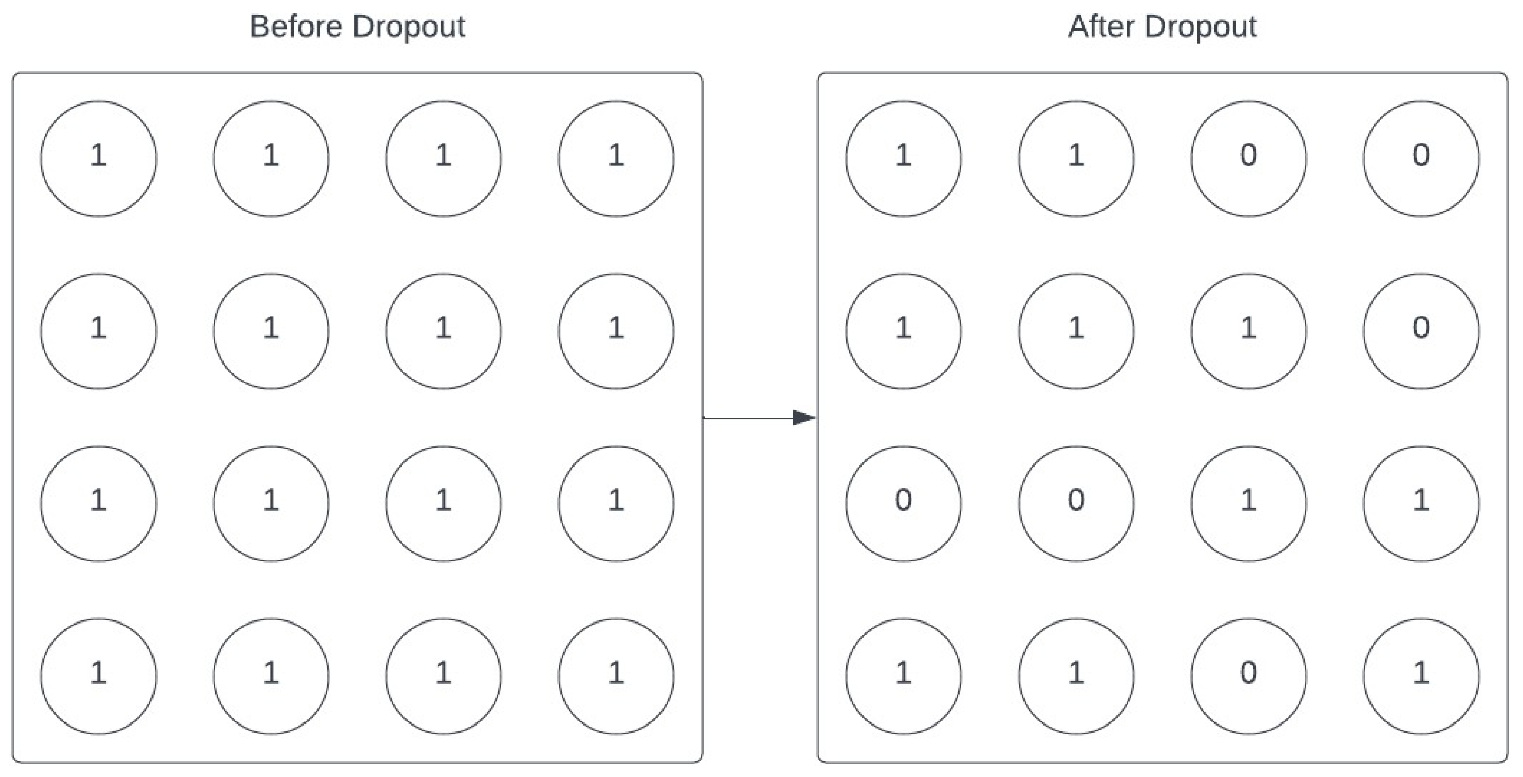
After the best optimizer was identified, the next series of experiments dealt with the architecture of the network itself, specifically regarding the addition of dropout layers to the network. In an LSTM network, and neural networks in general, dropout layers play a crucial role in mitigating overfitting and enhancing model generalization. Overfitting is a common challenge in LSTM networks due to their complex architectures and capacity to remember long-term dependencies. A dropout layer in an LSTM network functions by randomly deactivating a certain fraction of neurons in the network during the training phase. This process is visualized in Figure 2.
Figure 2.
Dropout visualization.
The effect of dropout in LSTMs is slightly different from traditional FNNs due to the recurrent connections. In LSTMs, dropout is usually applied only to non-recurrent connections, preserving the network’s ability to learn long-term dependencies. This selective application of dropout helps in regularizing the network without disrupting the flow of gradients through time. By randomly dropping out a subset of neurons, the LSTM network is forced to learn more robust features that are not reliant on the presence of specific neurons, thereby reducing the model’s sensitivity to particular neuron weights. This approach effectively simulates several different network architectures, promoting the development of a more generalized model. The results of varying dropout values are reported in Table 4. When the training is complete, the dropout layer is deactivated, allowing the full network to be utilized in the prediction phase. In addition to MAE and RMSE, the efficacy of the dropout layers is evaluated by the following metrics:
Table 4.
Results for one-hour forecast with differing epoch counts—Experiment 3.
- Mean Absolute Percentage Error (MAPE): A measure of prediction accuracy of a forecasting method, where the accuracy is typically expressed as a ratio.
- Mean Squared Error (MSE): The average squared distance between estimated values and the actual value.
- Coefficient of Determination (R2): The proportion of the variation in the dependent variable that is predictable from the independent variable(s).
The results show that the baseline model, without any dropout layers, establishes a benchmark for comparison. It exhibits a moderate balance across all metrics. However, the presence of relatively higher error rates suggests the potential for overfitting, highlighting the need for regularization. Introducing a dropout layer after the first LSTM layer shows varied effects. The dropout rate of 30% achieves the lowest MAE (47.04%) and MAPE (21.24%), indicating a slight improvement in predictive accuracy compared to the baseline. However, as the dropout rate increases to 50%, the errors slightly increase, implying a threshold beyond which increasing the dropout rate is counterproductive.
In the third test, using a dropout rate of 30% in a dropout layer after the second LSTM layer yields the best MAE (46.59%) and MAPE (21.52%) across all configurations, suggesting a more effective regularization than the first LSTM layer. However, using a dropout rate of 40% yields the best MSE (49.08%), RMSE (70.05%), and R2 (63.48%). Because the 40% dropout rate improves on three of the five metrics compared to a dropout rate of 30%, 40% is deemed the best-performing dropout rate for this test.
The combination of dropout layers after both LSTM layers does not significantly enhance performance. The configuration with 20% and 40% dropout rates results in an R2 score of 62.70%, which is lower than the highest achieved in the third test. This suggests that simultaneous dropout in both layers might not be as effective as selective dropout in either layer. Applying different dropout rates for the first layer, while keeping a constant 40% for the second, shows that higher dropout rates in the first layer led to increased errors. This indicates a diminishing return with higher dropout rates, especially when combined with a constant high dropout rate in the second layer.
The results of using different activation functions is shown In Table 5. For the first layer, the ReLU activation function shows relatively moderate MAE, MAPE, and R2 scores, indicating a balanced performance. Sigmoid, however, results in higher errors and lower R2 scores, suggesting less efficacy in this context. The Softmax function significantly underperforms, indicating its unsuitability for the first LSTM layer. The Softplus and Softsign functions perform comparably to ReLU, with Softsign showing slightly better results in some instances. The Tanh, SELU, and ELU functions exhibit a good balance between error metrics and R2 scores, with Tanh and ELU slightly outperforming SELU. The exponential activation function shows moderate performance but is not among the top performers.
Table 5.
Results of using different activation function configurations in the LSTM network.
Since ELU was the most effective activation function for the first layer, the second test simply demonstrates the efficacy of ELU for the second layer as well, before moving onto the third test, which examines alternative activation functions for the second layer.
Similar to the first test, ReLU demonstrated balanced performance, whereas sigmoid showed significantly higher errors. Both Softmax and Softplus continue to underperform in the second layer, with high errors and low R2 scores. Softsign, however, shows a notable improvement in the second layer, offering one of the best balances between the error metrics and R2 score. Tanh and SELU performed moderately well but without significant improvements over Softsign or ELU. The exponential function exhibited the poorest performance in the second layer, with the highest errors and lowest R2 score.
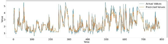
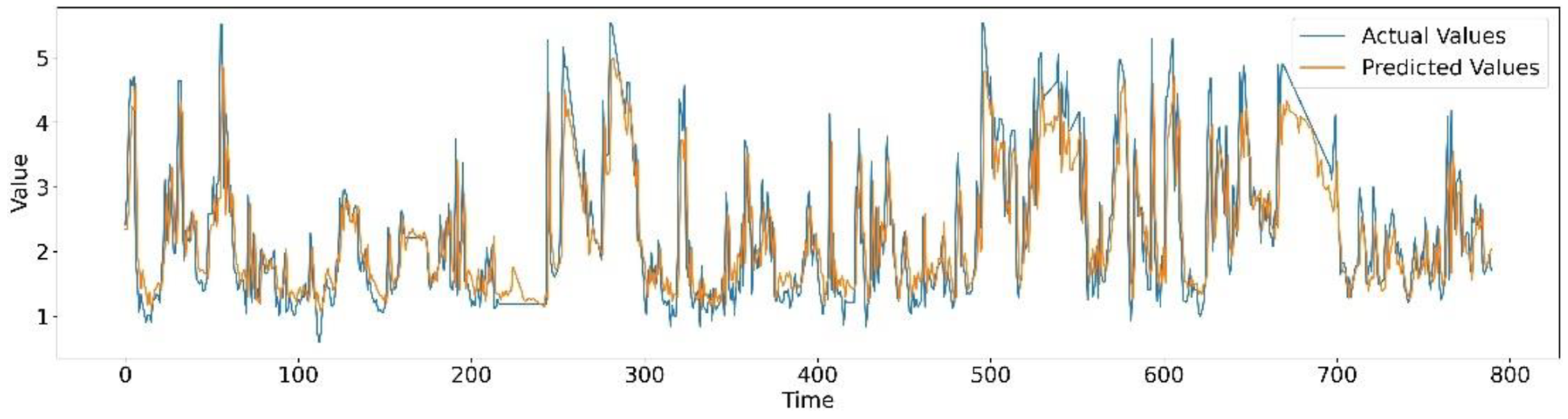
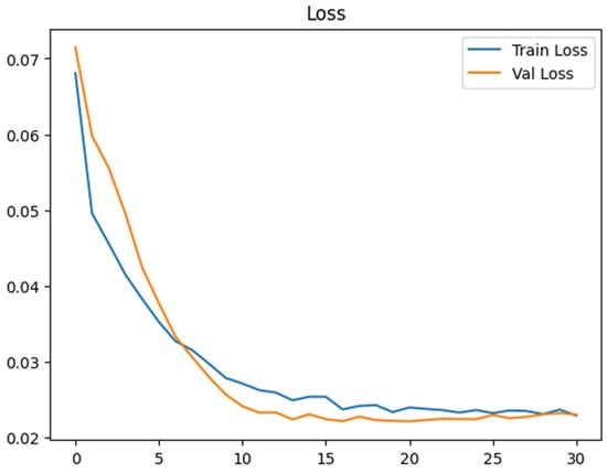
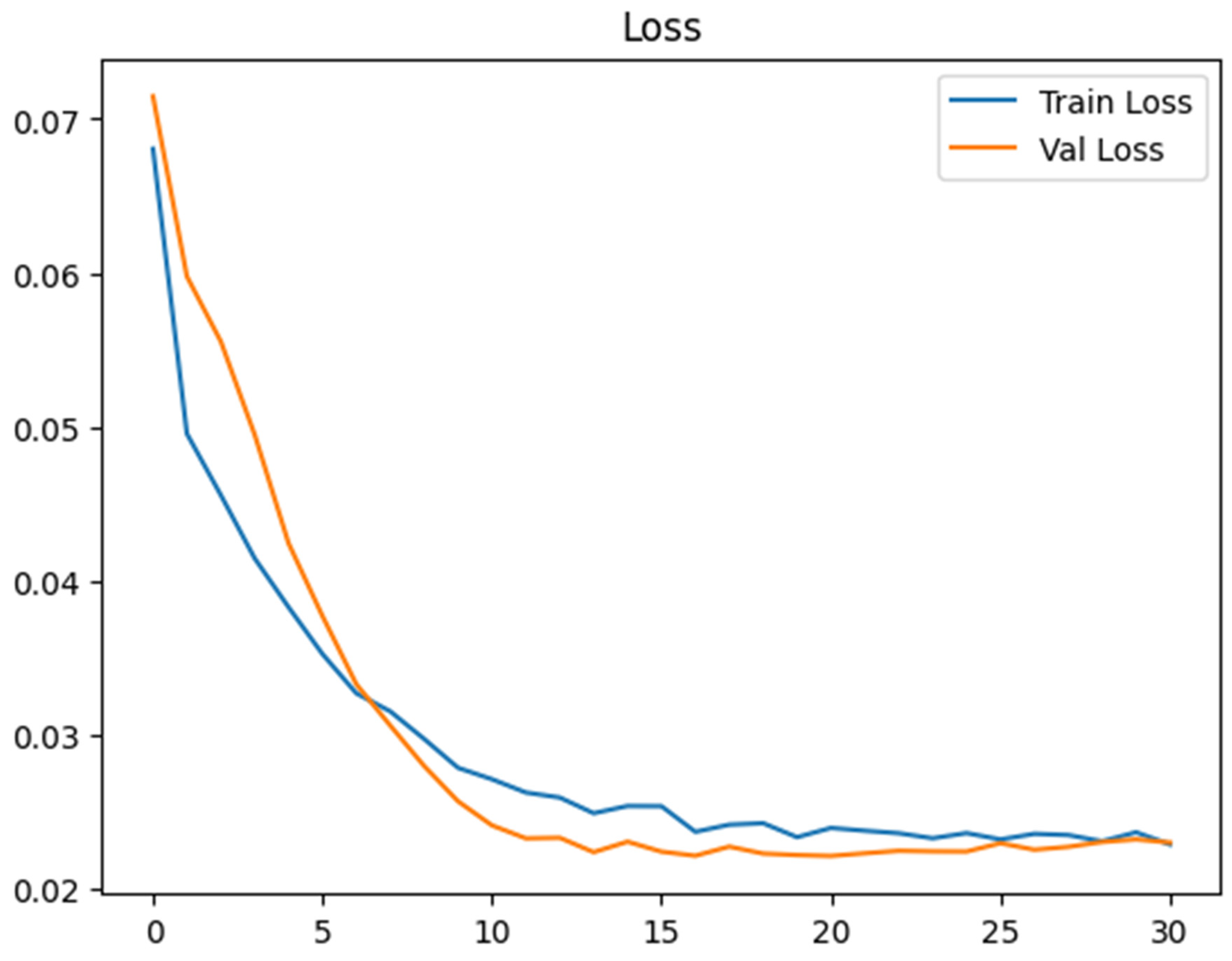
The final architecture of the LSTM network used in this study is shown in Figure 3. The predictive accuracies of the LSTM network compared to relevant baselines are listed in Table 6. The predicted versus actual values for silica content forecasting are shown in Figure 4. Figure 5 shows the training and validation curves for the final LSTM model.
Figure 3.
Final architecture of the LSTM network.
Table 6.
Accuracy metrics for the LSTM network vs. relevant baselines.
Figure 4.
Predicted vs. actual results over the span of hours.
Figure 5.
Training and validation curves for the LSTM model.
3.4. Data Interpolation
Once the results for predicting the silica content of the iron ore concentrate using the LSTM network were obtained, the focus shifted to predicting the silica content on a minute-by minute basis. Because the values for the purity of the concentrate in our dataset were recorded on an hourly basis, we interpolated the data to obtain values by minute. Data interpolation is a method for constructing new data points based on the range of a discrete set of known data points. The interpolation techniques used in this study are discussed below.
3.4.1. PCHIP Interpolation
The Piecewise Cubic Hermite Interpolating Polynomial (PCHIP) interpolation technique is a mathematical method for estimating data points within the range of a discrete set of known data points. Unlike other interpolation methods that may introduce unwanted oscillations or may not preserve the monotonicity of the data, PCHIP is designed to produce an interpolated curve that is smooth and visually appealing, while preserving the shape and trends of the data. This makes it particularly useful in cases where preserving data trends is important.
PCHIP achieves this using piecewise cubic polynomials between each pair of data points. These polynomials are determined in such a way that the interpolation is not only smooth, but also has continuous first derivatives, ensuring a smooth transition between segments. One key feature of PCHIP is its ability to maintain the monotonicity of the data; that is, if the data is increasing or decreasing, the interpolated curve will also increase or decrease between those data points, preventing the introduction of false local extrema.
In mathematical terms, given a set of data points (xi, y1) for i = 0, 1, …, n, PCHIP finds a cubic polynomial for the interval [xi, xi+1] that satisfies the following conditions:
- The polynomial passes through the data points at the ends of its interval;
- The first derivatives of the polynomials are continuous across the data points, ensuring that the curve is smooth;
- The monotonicity and convexity between each pair of data points are preserved in the interpolated curve.
PCHIP interpolation is widely used in applications where it is important to avoid overshooting and oscillations that can occur with other interpolation methods, such as spline interpolation, particularly when dealing with monotonic or nearly monotonic data. It is a popular choice in engineering, finance, and data visualization tasks, in which the accuracy of the trend is crucial.
3.4.2. Cubic Interpolation
Cubic spline interpolation is a form of spline interpolation in which piecewise cubic polynomials are used to interpolate a set of data points. This is a popular method for creating a smooth curve through a set of discrete points. The main goal of cubic spline interpolation is to obtain an interpolant that is smooth and continuous up to its second derivative across the entire range of data.
In more detail, suppose there is a set of n + 1 data points (x0, y0), (x1, y1), …, (xn, yn), where x0 < x1 < … < xn. Cubic spline interpolation seeks to find a cubic polynomial Si(x) for each interval [xi, xi+1], i = 0, 1, …, n − 1, such that:
- The spline interpolates the data points.
- The spine is continuous.
- The first and second derivatives of the spline are continuous across the range.
- Additional conditions are needed at the boundaries to determine the spline uniquely.
Cubic spline interpolation ensures a smooth, continuous curve that has a visually appealing form and is widely used in various applications, such as computer graphics, data interpolation, numerical simulation, and in any scenario where a smooth approximation of data is desirable.
3.4.3. Ensemble Interpolation
We present a simple ensemble interpolation technique that combines the PCHIP and cubic spline interpolation methods. For a given set of data points, we first independently performed both PCHIP and cubic spline interpolations to obtain two separate interpolating functions. Our ensemble method then computes the arithmetic mean of the PCHIP and cubic spline interpolants at each point in the domain to produce the final interpolated values. This straightforward averaging approach leverages the strengths of both methods, with PCHIP excelling at preserving the shape and monotonicity of the original data, whereas cubic splines tend to generate smoother interpolants. By taking the mean, our ensemble interpolation technique strikes a balance between faithful representation of the data trends and smoothness of the interpolating curve.
3.4.4. Evaluation of the Interpolation Techniques
To measure how our ensemble technique compares to the PCHIP and cubic spline techniques, we evaluated the performance based on several standard statistical tests and values:
- t-test: A type of statistical analysis used to compare the averages of two groups and determine whether the differences between them are more likely to arise from random chance.
- F-test: A statistical test used to compare the variances of two samples or the ratio of variances between multiple samples.
- Kolmogorov–Smirnov test: A nonparametric test of the equality of continuous one-dimensional probability distributions that can be used to compare a sample with a reference probability distribution or to compare two samples.
- t-statistic: The ratio of the departure of the estimated value of a parameter from its hypothesized value to its standard error.
- F-statistic: Used to determine if the tested data has an F-distribution under the true null hypothesis and true customary assumptions about the error term.
- Kolmogorov–Smirnov statistic: Quantifies the distance between the empirical distribution function and the cumulative distribution function of the reference distribution.
- p-value: The probability of obtaining test results at least as extreme as the result actually observed under the assumption that the null hypothesis is correct.
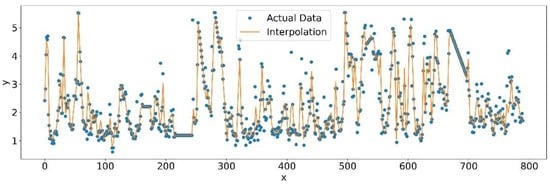
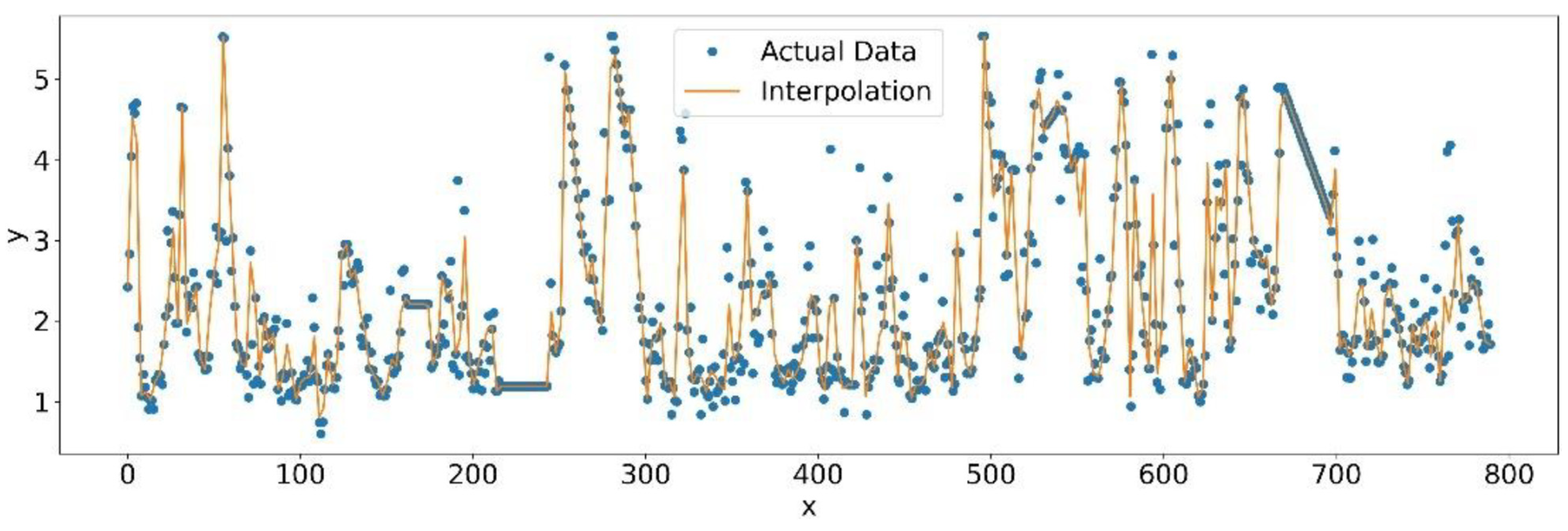
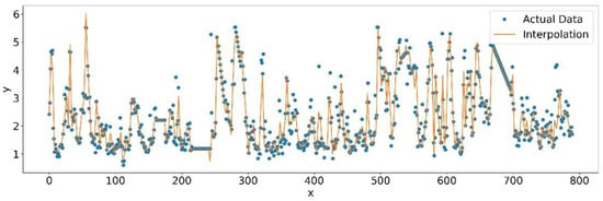
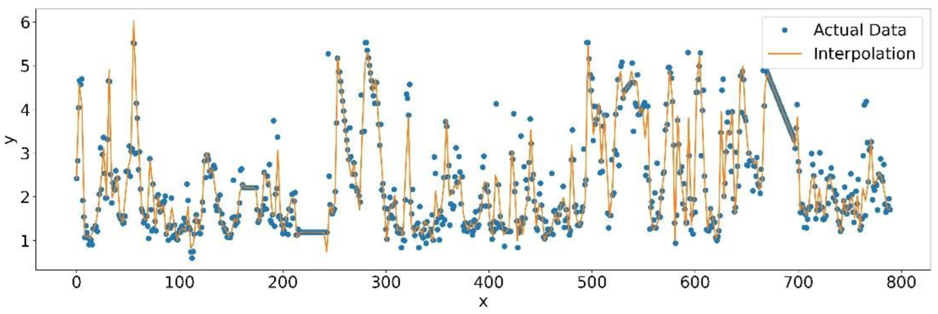
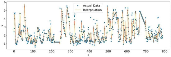
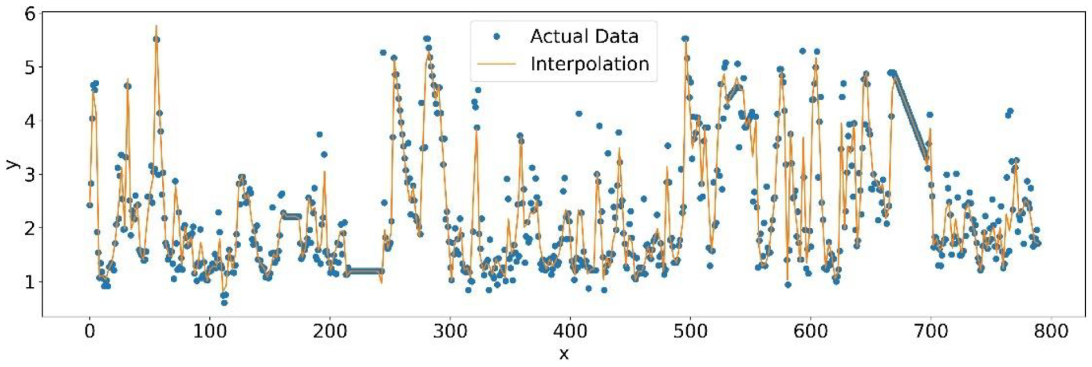
The results of these tests are listed in Table 7. Visualization of the interpolations are shown in Figure 5, Figure 6, Figure 7 and Figure 8.
Table 7.
Statistical analysis of the interpolation techniques.
Figure 6.
PCHIP interpolation results.
Figure 7.
Cubic spline interpolation results.
Figure 8.
Ensemble interpolation results.
The results show that our ensemble interpolation technique performs marginally better on both measured variables for the Kolmogorov–Smirnov test compared to PHIP and cubic spline while achieving a better t-statistic during the t-test than PCHIP, a better F-statistic during the F-test than cubic spline, and a better p-value during the F-test compared to PCHIP. However, the relatively high p-values observed across the t-test, F-test, and Kolmogorov–Smirnov test suggest that there is no statistically significant difference between the interpolation outputs at conventional significance levels. Instead, the findings suggest that the ensemble method provides a balanced interpolation that preserves the desirable properties of both PCHIP (trend preservation and monotonicity) and cubic splines (smoothness) while maintaining performance comparable to each individual method. This makes the ensemble approach a robust and reliable alternative, particularly in applications where stability and consistency across interpolation strategies are desirable.
4. Conclusions
In this study, we demonstrated the use of an LSTM network to capture and learn temporal patterns in mining data, enabling the prediction of silica content with high accuracy. The addition of the ensemble data interpolation technique further refines these predictions, ensuring that the model can operate effectively on a minute-by-minute basis despite the original hourly data frequency. This capability is crucial for operational decision-making, allowing for more precise control over the mining process and mitigation of potential issues related to ore quality.
The ensemble method introduced in this study offers a novel approach to data interpolation by balancing the strengths of both PCHIP and cubic spline methods. This ensures the preservation of data trends and smoothness, which is essential for accurate forecasting of silica content. Our comparisons with traditional interpolation methods validated the superiority of the ensemble technique in this context.
The combined use of an LSTM network and ensemble interpolation technique demonstrates the potential of machine learning applications in mining processes. Our approach not only enhances the prediction accuracy of important quality metrics, such as silica content, but also contributes to the broader goals of improving operational efficiency, reducing environmental impacts, and ensuring the sustainability of mining operations. Future work could explore the application of these techniques to other mining processes and the integration of additional predictive factors, potentially opening new avenues for optimization and control in the mining industry.
Author Contributions
Conceptualization, J.O.-M., T.W., K.J., C.I. and A.A.; methodology, T.W.; software, T.W.; validation, T.W. and G.B.; formal analysis, T.W. and G.B.; investigation, T.W.; resources, J.O.-M. and K.J.; data curation, T.W.; writing—original draft preparation, J.O.-M., T.W., K.J., C.I., A.A. and G.B.; writing—review and editing, J.O.-M., K.J., C.I. and A.A.; visualization, T.W.; supervision, J.O.-M. and K.J.; project administration, J.O.-M. and K.J.; funding acquisition, J.O.-M. and K.J. All authors have read and agreed to the published version of the manuscript.
Funding
This research received no external funding.
Institutional Review Board Statement
Not applicable.
Informed Consent Statement
Not applicable.
Data Availability Statement
The data utilized in this study were derived from the following resources available in the public domain: https://www.kaggle.com/datasets/edumagalhaes/quality-prediction-in-a-mining-process (accessed on 1 September 2024).
Conflicts of Interest
The authors declare no conflicts of interest.
References
- Fastmarkets. Iron Ore Indices: Methodology and Price Specifications—November 2025; Fastmarkets: London, UK, 2025. [Google Scholar]
- S&P Global Commodity Insights. Specifications Guide: Global Iron Ore; S&P Global Inc.: London, UK, 2024. [Google Scholar]
- Khatibisepehr, S.; Huang, B.; Khare, S. Design of inferential sensors in the process industry: A review of Bayesian methods. J. Process. Control. 2013, 23, 1575–1596. [Google Scholar] [CrossRef] [Scilit]
- McCoy, J.T.; Auret, L. Machine learning applications in minerals processing: A review. Miner. Eng. 2019, 132, 95–109. [Google Scholar] [CrossRef] [Scilit]
- Pural, Y.E. Developing a data-driven soft sensor to predict silicate impurity in iron ore flotation concentrate. Physicochem. Probl. Miner. Process. 2023, 59, 5. [Google Scholar] [CrossRef] [Scilit]
- Oda, J.; Akimoto, K.; Tomoda, T.; Nagashima, M.; Wada, K.; Sano, F. International comparisons of energy efficiency in power, steel, and cement industries. Energy Policy 2012, 44, 118–129. [Google Scholar] [CrossRef] [Scilit]
- Mei, Y.; Cheng, S.; Niu, Q.; Xu, W.; Ge, J. A review on transfer mechanism and influence factors of silicon in blast furnace. Ironmak. Steelmak. 2020, 47, 246–262. [Google Scholar] [CrossRef] [Scilit]
- Todoroki, H.; Mizuno, K. Effect of silica in slag on inclusion compositions in 304 stainless steel deoxidized with aluminum. ISIJ Int. 2004, 44, 1350–1357. [Google Scholar] [CrossRef] [Scilit]
- Lou, X.; Andresen, P.L.; Rebak, R.B. Oxide inclusions in laser additive manufactured stainless steel and their effects on impact toughness and stress corrosion cracking behavior. J. Nucl. Mater. 2018, 499, 182–190. [Google Scholar] [CrossRef] [Scilit]
- Podgornik, B.; Žužek, B.; Kafexhiu, F.; Leskovšek, V. Effect of Si content on wear performance of hot work tool steel. Tribol. Lett. 2016, 63, 5. [Google Scholar] [CrossRef] [Scilit]
- Singh, H. Effect of silica fume on steel slag concrete. Int. J. Innov. Res. Eng. Manag. 2022, 9, 35–40. [Google Scholar] [CrossRef] [Scilit]
- Birat, J.-P. Society, materials, and the environment: The case of steel. Metals 2020, 10, 331. [Google Scholar] [CrossRef] [Scilit]
- Ristovski, K.; Gupta, C.; Harada, K.; Tang, H.-K. Dispatch with confidence: Integration of machine learning optimization and simulation for open pit mines. In Proceedings of the 23rd ACM SIGKDD International Conference on Knowledge Discovery and Data Mining (KDD ’17), Halifax, NS, Canada, 13–17 August 2017. [Google Scholar]
- Lee, C.; Kim, S.-M.; Choi, Y. Case analysis for introduction of machine learning technology to the mining industry. Tunn. Undergr. Space 2019, 29, 1–11. [Google Scholar]
- Zelinska, S. Machine learning: Technologies and potential application at mining companies. E3S Web Conf. 2020, 166, 03007. [Google Scholar]
- Jung, D.; Choi, Y. Systematic review of machine learning applications in mining: Exploration, exploitation, and reclamation. Minerals 2021, 11, 148. [Google Scholar] [CrossRef] [Scilit]
- Fu, Y.; Aldrich, C. Deep learning in mining and mineral processing operations: A review. IFAC-Pap. 2020, 53, 11920–11925. [Google Scholar] [CrossRef] [Scilit]
- Paduraru, C.; Dimitrakopoulos, R. Responding to new information in a mining complex: Fast mechanisms using machine learning. Min. Technol. 2019, 128, 129–142. [Google Scholar] [CrossRef] [Scilit]
- Ali, D.; Frimpong, S. Artificial intelligence, machine learning and process automation: Existing knowledge frontier and way forward for mining sector. Artif. Intell. Rev. 2020, 53, 6025–6042. [Google Scholar] [CrossRef] [Scilit]
- Jooshaki, M.; Nad, A.; Michaux, S. A systematic review of the application of machine learning in exploiting mineralogical data in mining and mineral industry. Minerals 2021, 11, 816. [Google Scholar] [CrossRef] [Scilit]
- Chetan Kumar, G.S.; Kavana, K.M. Iron ore quality prediction using machine learning. Int. J. Sci. Res. Eng. Manag. 2022, 6, 1–5. [Google Scholar]
- Quality Prediction in a Mining Process. Kaggle. Available online: https://www.kaggle.com/datasets/edumagalhaes/quality-prediction-in-a-mining-process/ (accessed on 2 March 2026).
- Khayati, M.; Lerner, A.; Tymchenko, Z.; Cudré-Mauroux, P. Mind the gap: An experimental evaluation of imputation of missing values techniques in time series. Proc. VLDB Endow. 2020, 13, 768–782. [Google Scholar] [CrossRef] [Scilit]
- Li, J.; Cheng, K.; Wang, S.; Morstatter, F.; Trevino, R.P.; Tang, J.; Liu, H. Feature selection: A data perspective. ACM Comput. Surv. 2017, 50, 1–45. [Google Scholar] [CrossRef] [Scilit]
- Hall, M.A. Correlation-Based Feature Selection for Machine Learning. Ph.D. Thesis, The University of Waikato, Hamilton, New Zealand, 1999. [Google Scholar]
- Pu, Y.; Szmigiel, A.; Apel, D.B. Purities prediction in a manufacturing froth flotation plant: The deep learning techniques. Neural Comput. Appl. 2020, 32, 13639–13649. [Google Scholar] [CrossRef] [Scilit]



Disclaimer/Publisher’s Note: The statements, opinions and data contained in all publications are solely those of the individual author(s) and contributor(s) and not of MDPI and/or the editor(s). MDPI and/or the editor(s) disclaim responsibility for any injury to people or property resulting from any ideas, methods, instructions or products referred to in the content. |
© 2026 by the authors. Licensee MDPI, Basel, Switzerland. This article is an open access article distributed under the terms and conditions of the Creative Commons Attribution (CC BY) license.