


Abstract
The adjustable speed hydro-generating unit has a complex three-phase alternating current excitation structure. The existing rotor winding short circuit (RWSC) fault diagnosis methods are generally difficult to use to locate the fault location and identify the severity of the fault. Therefore, an offline diagnosis method for the internal RWSC of an adjustable speed hydro-generating unit is proposed in this paper. Firstly, after the unit is shut down, the low-voltage pulse signal is repeatedly injected into the rotor winding by the pulse generator. By comparing and analyzing the voltage response characteristics under different types of short circuit faults, an identification method of rotor winding short circuit fault type and fault phase based on detecting the reverse polarity sub-spike is proposed. Furthermore, the short circuit fault point can be accurately located by combining ensemble empirical mode decomposition (EEMD) with the Teager energy operator (TEO). Finally, the fault factor is constructed based on the area between the characteristic waveform and the zero line, and the quantitative evaluation of the severity of the short circuit fault is realized based on this. The effectiveness of the proposed fault diagnosis and location method is verified by the simulation results.
1. Introduction
Pumped storage is a clean and flexible regulating power source with the best economy and the most large-scale development potential, which can provide important assistance for the realization of the “double carbon” strategic goal and the construction of new power systems [1,2]. Compared with the constant speed hydro-generating unit, the adjustable speed hydro-generating unit based on alternating current excitation has the advantages of a wider operating range and higher efficiency, which can more effectively absorb new energy power generation and improve the anti-interference ability of the power grid [3,4].
The adjustable speed hydro-generating unit uses three-phase alternating current excitation, and its rotor winding structure, short circuit fault type, and fault characteristics are more complicated than those of the constant speed hydro-generating unit [5]. When the rotor winding of an adjustable speed hydro-generating unit is short circuited, it is easy to have problems such as rising winding temperature and abnormal vibration of the unit. In severe cases, it may even burn the rotor winding [6,7]. Therefore, accurate diagnosis of the rotor winding short circuit (RWSC) fault, fault location, and fault degree are of great significance to shorten the troubleshooting time and improve the safety and stability of the unit [8].
The existing RWSC fault diagnosis methods of adjustable speed hydro-generating units can be broadly categorized into two types: one type is the online diagnosis method, and the other type is the offline diagnosis method, which have their own advantages and disadvantages. For the online diagnosis method, reference [9] realized the protection of rotor winding short circuit based on the total effective value of stator zero sequence transverse differential current harmonics, but this method has the risk of misoperation when a short circuit fault occurs inside the stator winding. In reference [10], the total effective value of the stator transverse differential current harmonics is combined with the ratio differential protection to realize the rotor winding short circuit protection. However, this method has a risk of failure to operate for some small-shorted-turn faults and a few large-shorted-turn faults. Reference [11] used the zero-sequence current component to realize the detection and location of the ITSC of the rotor winding. However, it is insensitive to minor winding faults, which may lead to missed detection. Reference [12] proposed a rotor winding fault diagnosis and location method based on current residuals, but its location accuracy is low, and the location of the fault coil cannot be determined.
For the offline diagnosis method, reference [13] proposed to apply the recurrent surge oscillography (RSO) to the offline detection of the ITSC fault of the generator rotor winding. In reference [14], the fault feature set is combined with the residual BP neural network to establish the mapping relationship between the fault feature and the fault location, and the transformer short circuit fault diagnosis is realized. However, the application scenario of the above method is relatively simple, and it is mostly applied to the ITSC fault diagnosis of generators or transformers, which is not suitable for an adjustable speed hydro-generating unit with three-phase alternating current excitation of rotor winding. Reference [15] combined the convolutional neural network with the transformer architecture to realize the fault diagnosis of the doubly-fed induction generator. However, this method requires a large number of training samples, and the engineering practice is weak. In Reference [16], rotor winding fault detection is realized by injecting voltage into the rotor winding through the rotor-side inverter. However, this method focuses on the fault diagnosis of small-capacity doubly fed wind turbines, and it is difficult to apply to large-capacity adjustable speed hydro-generating units. Reference [17] adopts the frequency response analysis method to realize the fault diagnosis of rotor winding. However, it has weak anti-interference ability, which may lead to misjudgment in engineering practice. For this reason, reference [18] improved the traditional RSO and proposed a maximum spike time difference detection method suitable for adjustable speed hydro-generating units. However, this method may cause misjudgment of the fault type when the fault location is near to the neutral point. The advantage of the offline diagnosis method is the fault location and fault degree identification after the fault shutdown [19,20]. It should be noted that there is no conflict between offline diagnosis and online diagnosis. Offline diagnosis is a functional extension of online diagnosis, and the two should be applied together [21].
Therefore, this paper proposes an RSO suitable for the rotor winding structure of an adjustable speed hydro-generating unit. This method can not only accurately identify the internal short circuit fault type of the rotor winding, but also accurately locate the fault location. This method is implemented in the environment where the unit is completely disconnected from the power grid, and there is no power frequency electrical signal or strong electromagnetic interference. Only by injecting low-voltage pulses into the rotor winding and collecting the port voltage response can the internal short circuit fault type of the rotor winding be accurately identified and the severity of the fault can be evaluated. At the same time, the ensemble empirical mode decomposition (EEMD) algorithm and the Teager energy operator (TEO) algorithm can filter out clutter and noise interference and amplify the transient characteristics of fault traveling waves [22,23,24,25]. It can also effectively resist the influence of non-ideal conditions such as acquisition error and winding parameter dispersion, ensure the accuracy and stability of fault location, and realize the accurate locking of fault location, with excellent robustness and anti-interference ability [26,27,28,29,30]. It should be noted that for serious short circuit faults, the existing relay protection can only trip quickly after the fault occurs, avoiding the expansion of the fault and damage to the unit’s equipment [31]. However, due to the limitation of the principle, it is impossible to distinguish the fault type and accurately locate the fault location. The rotor winding structure of a large-capacity adjustable speed hydro-generating unit is complex, and the lack of accurate fault information will lead to a long maintenance cycle, high cost, and significant downtime loss [32]. The method proposed in this paper can not only greatly shorten the maintenance time and reduce economic losses but also support fault root cause analysis and preventive operation and maintenance, which effectively makes up for the shortcomings of existing methods and relay protection and has outstanding engineering practical value [33].
The rest of this paper is organized as follows: Section 2 aims at the problem that the existing offline diagnosis method is difficult to apply directly to an adjustable speed hydro-generating unit; a fault diagnosis method based on the detection of the reverse polarity sub-spike is proposed in combination with the structural characteristics of the rotor winding of adjustable speed hydro-generating unit. Section 3 presents an accurate fault location method for internal RWSC faults in adjustable speed hydro-generating units, based on the combination of EEMD and the TEO. In Section 4, considering that the spread of traveling waves in the winding is attenuated, which will cause a certain degree of distortion of the characteristic waveform, a fault factor is proposed to quantitatively evaluate the short circuit fault based on the area between the characteristic waveform and the zero line. Section 5 presents the conclusions.
2. Internal RWSC Identification Method
2.1. Analysis of Internal RWSC Fault Diagnosis Principle
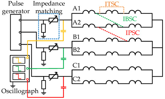
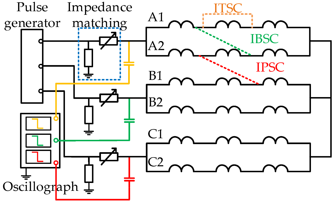
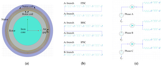
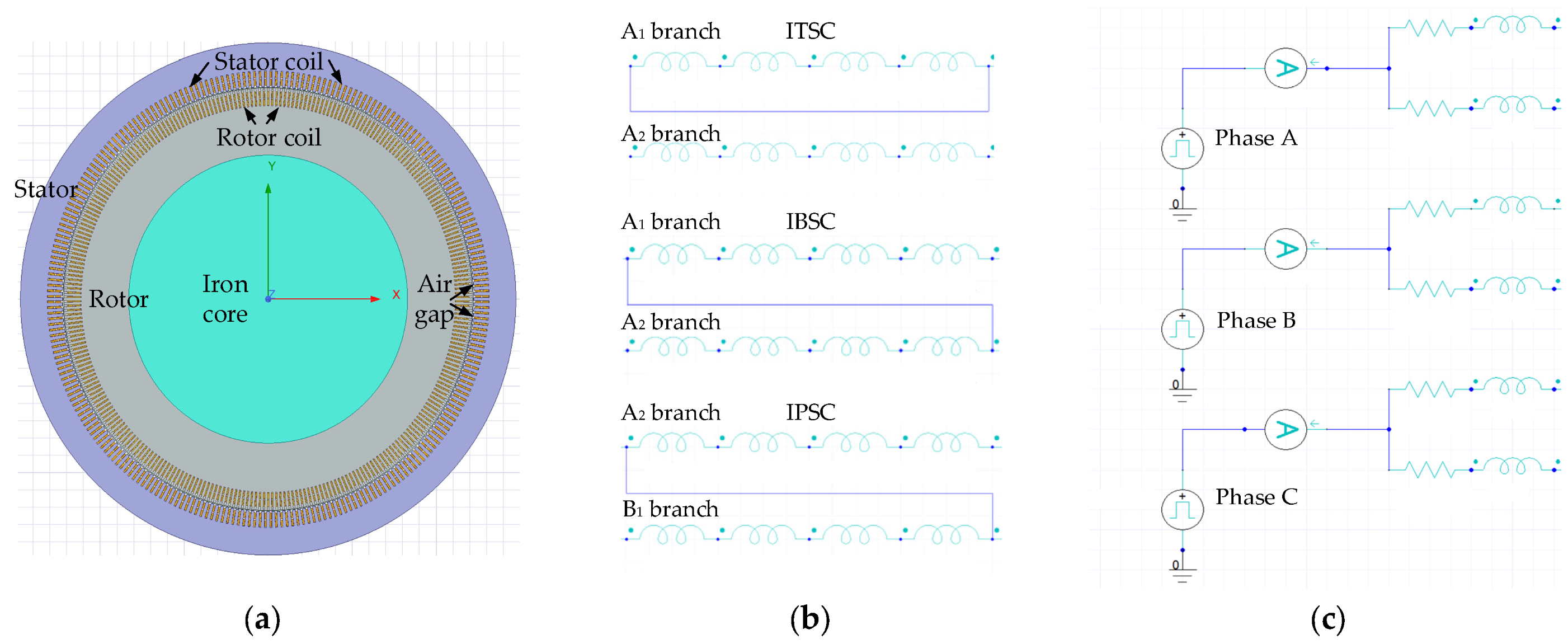
Taking the adjustable speed unit of a 300 MW hydro-generating power station as an example, the detailed parameters are shown in Table 1. The internal RWSC fault has three types: ITSC, inter-branch short circuit (IBSC), and inter-phase short circuit (IPSC), as shown in Figure 1. The rotor of the adjustable speed unit adopts three-phase alternating current excitation. Each phase contains two branches, and the branches are in parallel structures. Each branch contains 49 coils, and the coils are in a series structure. The length of each coil is 10.500 m, and the form of the winding is dual-layer ripple winding. The RWSC fault model of an adjustable speed hydro-generating unit is established and simulated in ANSYS Maxwell 2022 R2. The unstructured adaptive grid scheme and the second-order tetrahedral element are used to model. The grid sensitivity analysis shows that the simulation results can effectively eliminate the interference of grid density. The details of simulation modeling are shown in Figure 2. The finite element model of the motor can take into account the key factors such as electromagnetics and structure through refined multiphysical field modeling and consider the coupling effect between different phase windings and the influence of coupling between windings on the wave process. It should be noted that the coil length is composed of a straight line effective section embedded in the core slot with a length of 10 m and an end connection section at both ends of the winding with a length of 0.5 m. The fault length in the modeling and expression in this paper specifically refers to the total length of the straight line effective section in the slot of all series windings that are short circuited. The nomenclature of symbols used in this paper is specified in Table A1 of Appendix A.
Table 1.
Simulation model parameters.
Figure 1.
RSO diagnosis diagram of an adjustable speed hydro-generating unit.
Figure 2.
Schematic diagram of simulation modeling: (a) Top view of motor used in simulation; (b) Setting method of short circuit fault; (c) Injected pulse.
After the unit is shut down, the pulse signal is repeatedly injected into the rotor winding by the pulse generator, and each time it is injected into two different phases three times. Specifically, inject into phases A and B, inject into phases B and C, and inject into phases A and C, and set signal acquisition points at the ends of each phase. Based on the traveling wave theory, the catadioptric process of the signal will occur when the pulse signal impedance is discontinuous at the short circuit point. In this scheme, the characteristic curve is obtained by calculating the difference of the voltage response waveform of the two phases injected each time, and there are three characteristic curves. Then, the internal RWSC is identified according to the obtained characteristic curve. Because the rotor structure of the adjustable speed hydro-generating unit is three-phase symmetrical, the three characteristic curves obtained during normal operation are all zero lines.
2.2. Response Characteristics of ITSC
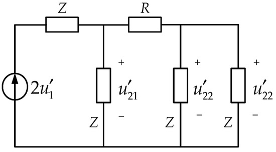
The ITSC point can be regarded as a resistance R (short circuit fault resistance); two parallel lines with the same wave impedance Z are connected on each side of it. Based on Peterson’s law and combined with the ITSC fault, the equivalent circuit shown in Figure 3 can be obtained. The forward wave is refracted and reflected at two fault points at the same time. The relationship between the reflected wave voltage, the refracted wave voltage, and the forward wave is shown in Equations (1)–(3).
where is the forward wave voltage; and are the reflected wave voltage and the refracted wave voltage of at the short circuit point of the near injection side; is the refracted wave voltage at the short circuit point of the far injection side.
Figure 3.
ITSC equivalent circuit.
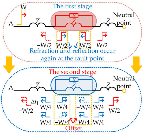
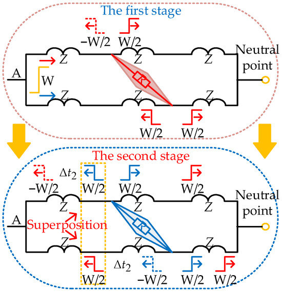
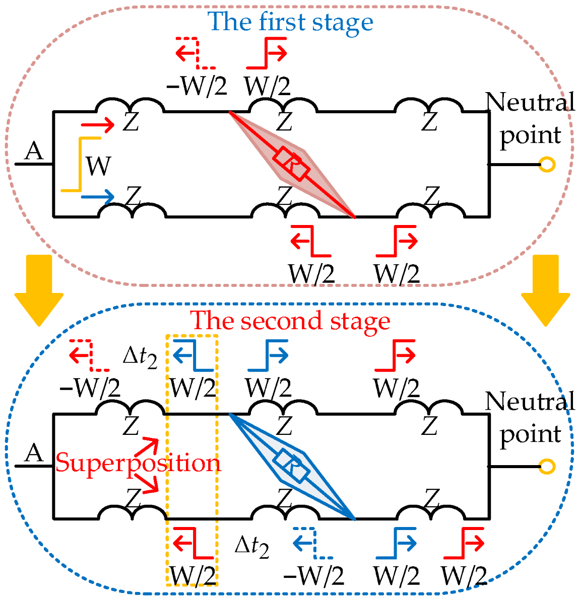
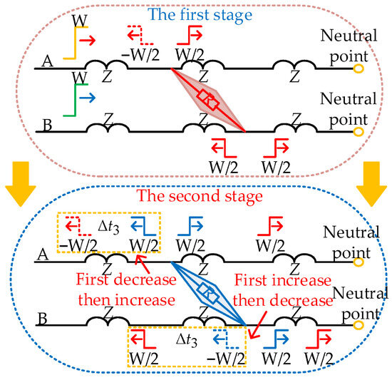
Considering that the fault resistance R is usually lower than the wave impedance Z in the RWSC fault, this will be more apparent in the situation of IPSC. Therefore, , , can be approximately obtained. The branch of the fault-free point in the non-fault phase and the fault phase is omitted, and the catadioptric process of the wave during the ITSC is shown in Figure 4, where “W” represents the amplitude of the incident wave. Taking the ITSC fault of phase A as an example, the pulse is injected into phases A and B. The catadioptric process of phase A injection pulses at the fault point can be separated into two stages.
Figure 4.
Catadioptric diagram of wave in ITSC.
The positive half-period square wave pulse is taken as an example for analysis. In the first stage, the pulse injected in phase A is refracted and reflected when it reaches the short circuit point of the near injection side, generating a negatively polarized reflected wave with an amplitude of 1/2 of the incident wave and three positively polarized refracted waves with an amplitude of 1/2 of the incident wave. After passing through (the travel time of the wave along the short circuited winding), the process enters the second stage. The two refracted waves generated in the short circuited winding during the first stage simultaneously reach the short circuit point near the injection side and the short circuit point far from the injection side, respectively, and undergo the aforementioned refraction and reflection again. The reflected and refracted waves are identical in amplitude but opposite in polarity, leading to mutual offset. As a result, two refracted waves persist in the second stage, traveling toward the winding head end and the neutral point.
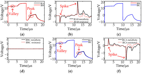
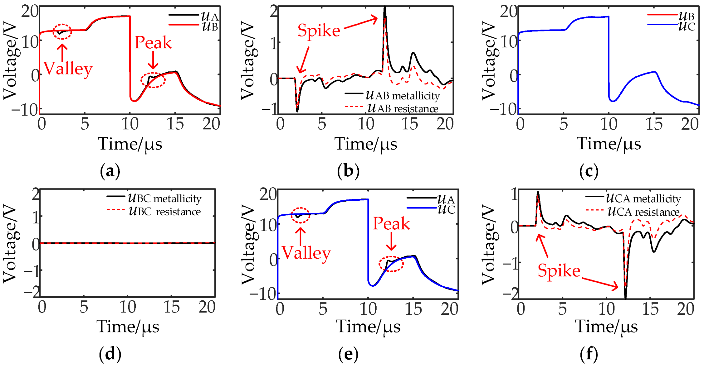
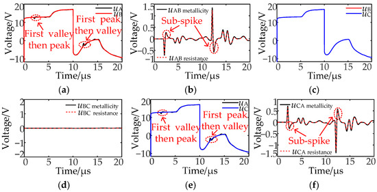
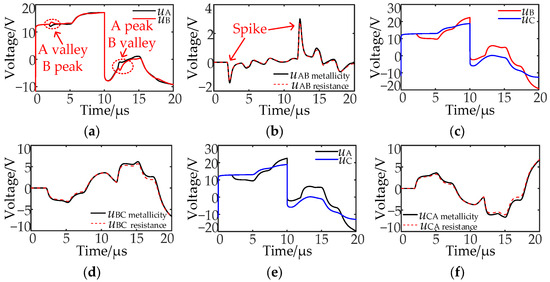
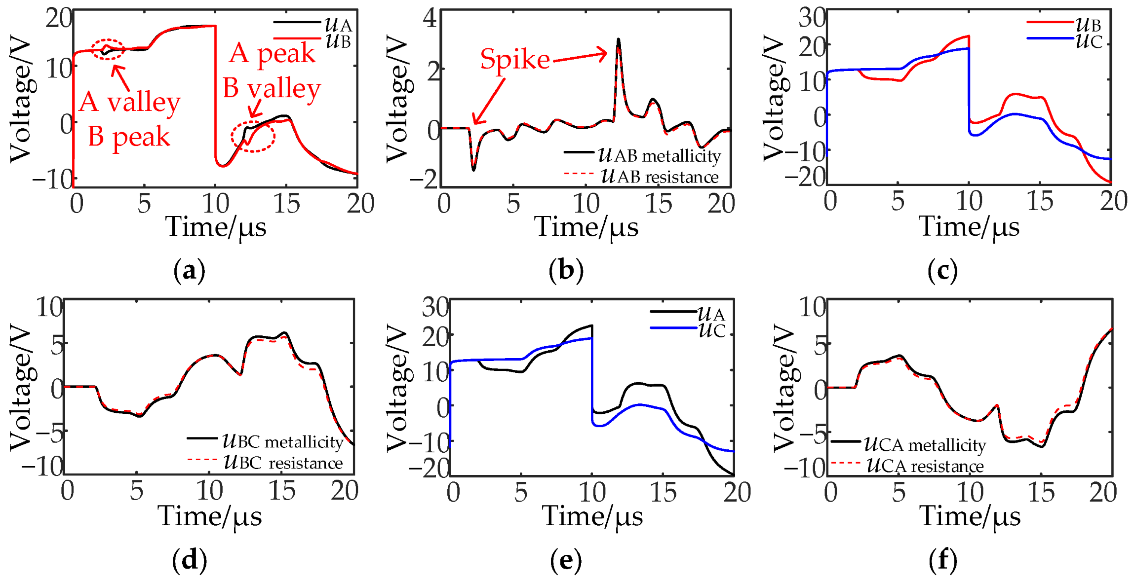
When the pulse is injected into phases A and B or phases A and C, the reflected wave generated by the phase A injection pulse in the first stage is negative polarity, followed by two second-stage refraction waves. The amplitude of the wave synthesized by the two is equal in magnitude to that of the reflected wave, with opposite polarity, and the time lag is . It can be seen from Figure 4 that the misalignment of the two waveforms causes the voltage response waveform of phase A to first decrease and then increase, forming a valley, as shown in Figure 5a,e. On the contrary, when the square wave is in its negative half cycle, it will form a peak. When there is a valley or a peak in the voltage response waveform, there will be a spike in the characteristic waveform. The spike is a point or region with a local maximum value.
Figure 5.
Voltage response characteristics of ITSC: (a) uA and uB; (b) uAB; (c) uB and uC; (d) uBC; (e) uA and uC; (f) uCA.
2.3. Response Characteristics of IBSC
Taking the IBSC of phase A as an example, the pulse is injected into phases A and B. The catadioptric process of the fault phase injection pulse at the fault point is also divided into two stages, and the sound phase is omitted. The catadioptric process is shown in Figure 6. Taking the positive half cycle of a square wave as an example for analysis. In the first stage, the positive half-cycle square wave pulse injected in phase A will reach the short circuit point on the near injection side and undergo a catadioptric process, the number of refracted and reflected waves generated and their relationship with the forward wave are the same as those of the ITSC described before. After passing through (the travel time of the wave between the two branch short circuit points), the process enters the second stage. The injection pulse reaches the far injection side short circuit point from the other branch and undergoes the same catadioptric process.
Figure 6.
Catadioptric diagram of a wave in IBSC.
When the pulse is injected into phases A and B or phases A and C, the negative polarity reflected wave generated by the phase A injection pulse in the first stage will be first detected. After , the positive refraction waves generated in the first and second stages towards the winding head end will arrive at the detection point at the same time. After a further , the negative reflection wave generated in the second stage will also reach the first end, and the amplitude of each catadioptric wave is 1/2 of the incident wave. Therefore, the phase A voltage response waveform will first decrease, then increase, and then decrease, and each change is separated , as shown in Figure 7a,e, valley and peak appear one after another. The situation is the opposite when the square wave is in its negative half-cycle. When the valley and the peak appear one after another, the characteristic waveform will first appear as a spike, followed by a reverse polarity sub-spike. The reverse polarity sub-spike refers to the first local extreme point that appears immediately after the main spike, which is opposite to the polarity of the main spike. When the pulse is injected into phases B and C, uB is the same as uC, and uBC is a zero line.
Figure 7.
Voltage response characteristics of IBSC: (a) uA and uB; (b) uAB; (c) uB and uC; (d) uBC; (e) uA and uC; (f) uCA.
2.4. Response Characteristics of IPSC
Taking the IPSC between phases A and B as an example, the pulse is injected into phases A and B, and the catadioptric process of the wave is also divided into two stages. The branches without fault points in the non-fault phase and the fault phase are omitted, and the catadioptric process is shown in Figure 8.
Figure 8.
Catadioptric diagram of wave in IPSC.
Taking the positive half cycle of the square wave as an example for analysis. In the first stage, the phase A pulse first reaches the short circuit point near the injection side, and refraction occurs, which is similar to the above-mentioned IBSC. After passing through (the travel time of the wave between the two phase short circuit points), the process enters the second stage, and the phase B pulse will reach the short circuit point on the far injection side and refract and reflect. The phase A voltage response waveform will first decrease and then increase, and there will be a valley; the phase B voltage response waveform will first increase and then decrease, and there will be a peak, as shown in Figure 9a. The situation is the opposite when the square wave is in its negative half-cycle.
Figure 9.
Voltage response characteristics of IPSC: (a) uA and uB; (b) uAB; (c) uB and uC; (d) uBC; (e) uA and uC; (f) uCA.
When the pulse is injected into phases B and C or phases A and C, the fault phase injection pulse will occur multiple refractions and reflections at the two fault points and the neutral point. Thus, the voltage response waveforms of the fault phase and non-fault phase exhibit a significant difference; the amplitude of the characteristic waveform uBC and uCA is larger than the amplitude of the characteristic waveform uAB.
2.5. Internal RWSC Fault Type Identification
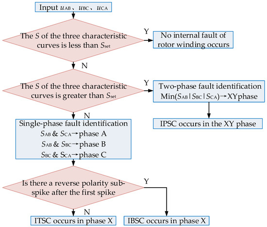
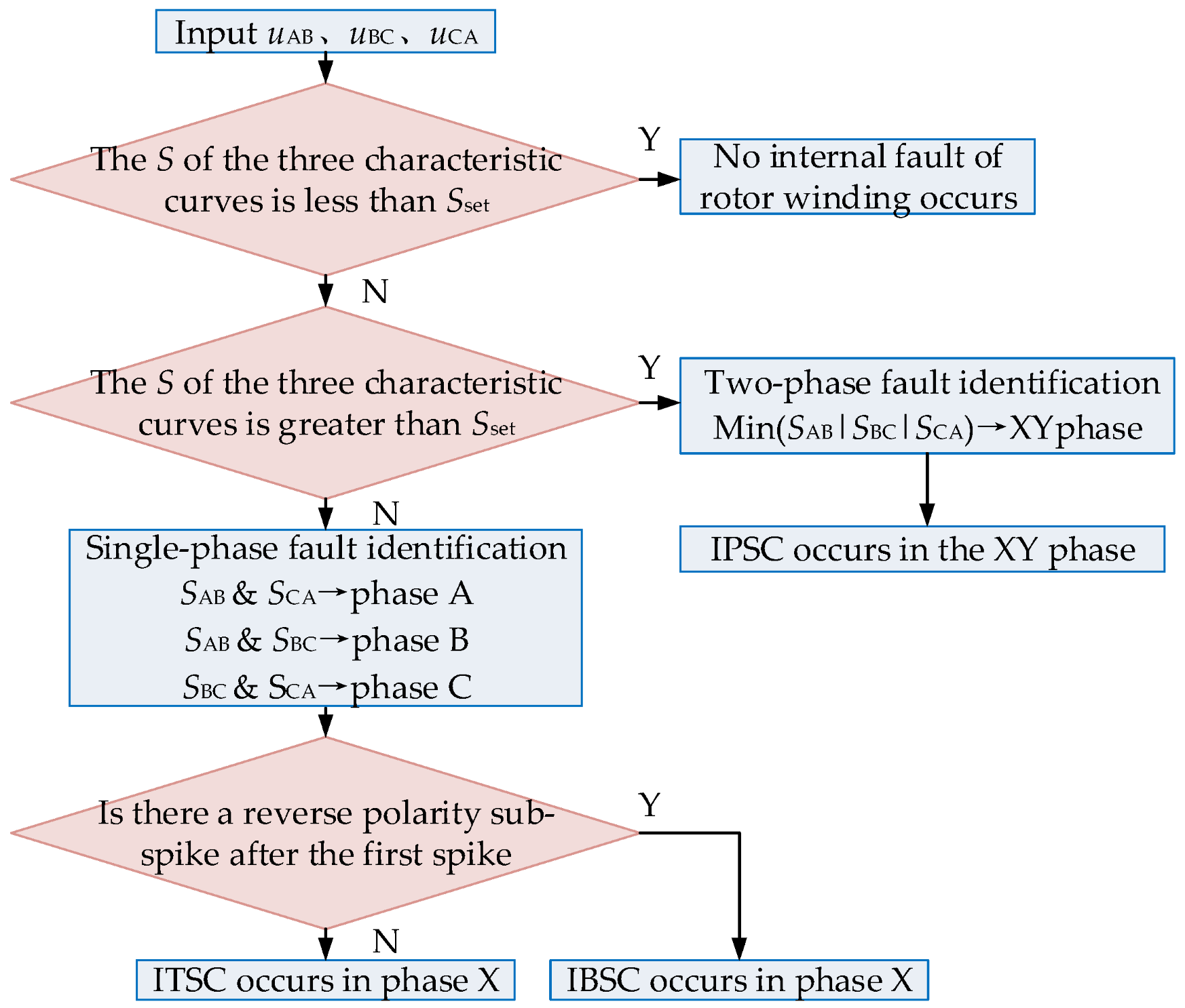
When the RWSC fault occurs, the fault characteristics of the IPSC are obvious, and it is easy to distinguish it from the ITSC and the IBSC. The fault characteristics of the ITSC and the IBSC are very close, and it is difficult to distinguish them. Therefore, this paper adopts the area enclosed by the characteristic waveform and the zero line as the fault factor and proposes a fault type identification method based on detecting the reverse polarity sub-spike. The specific process is shown in Figure 10, and Equations (4) and (5) are the calculation and setting methods of fault identification parameters, respectively.
where u(t) is the characteristic waveform, ts is the start time of u(t), te is the end time of u(t), S is the fault identification parameter, and its unit is V·μs.
where Sset is the setting value of the fault identification parameter, k is the setting coefficient and 0 < k ≤ 1; G is the amplitude of the injected pulse. To ensure the correct identification of the fault type under remote high resistance fault conditions in practical engineering, k is set to 0.025 in this paper, i.e., the setting value Sset is 0.5 V·μs.
Figure 10.
Process of RWSC fault type identification method.
To avoid the missed diagnosis of the remote high resistance fault when the set value Sset is too large, the fault misdiagnosis occurs when the set value Sset is too small. Equation (6) can be used for sensitivity verification.
where q is the minimum fault identification sensitivity; Smin is the minimum value among the calculated fault identification parameters that are greater than Sset. In general, q > 1.2 can ensure the correct identification of the fault type under the remote high resistance fault.
(1) Determine the number of S in the three characteristic curves greater than Sset. If the S of the three characteristic curves is less than Sset, there is no fault in the rotor winding.
(2) If the S of the three characteristic curves is greater than Sset, the type of fault can be judged as the IPSC, and the two phases corresponding to the one with the smallest S among the three characteristic curves are the faulty phases.
(3) If the above two judgments are not satisfied, there must be only two characteristic curves with S greater than Sset. The one phase shared by the two is the fault phase, and the fault type is ITSC or IBSC.
(4) For the two characteristic curves with S greater than Sset, if the first spike is not immediately followed by a sub-spike of opposite polarity, the fault is determined as an ITSC; otherwise, it is determined as an IBSC.
The calculated value of S under a remote high resistance fault is shown in Table 2. It can be seen that the method proposed in this paper can accurately identify the fault phase and fault type by judging the number of S calculated values greater than Sset even under the harsh conditions that the fault point is 400 m away from the winding head end and the fault resistance is 200 Ω, which proves the effectiveness of the fault identification method proposed in this paper.
Table 2.
The calculated value of S under a remote high resistance fault.
The calculated value of S under a remote high resistance fault is shown in Table 2. According to Equation (6), the minimum fault identification sensitivity can be calculated to be 2.188 under the harsh condition that the fault point is 400 m away from the winding head end and the fault resistance is 200 Ω. The fault phase and fault type can be accurately identified, which proves the effectiveness of the fault identification method.
3. Fault Location
3.1. Fault Location Algorithm
On the basis of fault type identification, accurate fault location enables field maintenance personnel to rapidly identify the fault and implement corresponding treatment measures. To this end, this paper develops an EEMD-TEO-based fault location method.
As a modified empirical mode decomposition method, EEMD introduces Gaussian white noise in multiple decomposition processes, taking advantage of its statistical property with uniform frequency distribution. In each round of decomposition, different white noise with the same amplitude is added to change the extremum characteristics of the signal. Subsequently, the corresponding intrinsic mode function (IMF) obtained from multiple empirical mode decompositions (EMDs) is averaged to offset the introduced white noise, thereby effectively suppressing the generation of mode aliasing [34,35,36,37]. The number of decomposition layers of EEMD used in this paper is 10; the noise intensity is 0.100 times the original signal; the average number of sets is 100. The decomposition steps are as follows:
(1) Set the overall average number of times as N.
(2) A new signal is constructed by introducing white noise that follows the standard normal distribution into the original signal.
where ni(t) is the Gaussian white noise added in the ith time; x(t) is the original signal; xi(t) is the additional noise signal of the ith test, .
(3) The obtained signal with noise is decomposed by EMD, and the form of the sum of each IMF is obtained.
where ci,j(t) is the jth IMF obtained by the decomposition of the ith time after adding white noise, ri(t) is the residual function, which represents the average trend of the signal, M is the number of IMFs.
(4) Steps (2) and (3) are repeated N times, and white noise signals with different amplitudes are introduced in each decomposition to obtain a set of IMFs.
(5) By using the principle that the statistical average value of the uncorrelated sequence is zero, the corresponding IMFs are averaged to obtain the final IMF after EEMD decomposition.
where cj(t) is the jth IMF of EEMD decomposition and r(t) is the final residual function, , .
TEO is a nonlinear difference operator, which has a small amount of computation, high time resolution, and good adaptive ability to the instantaneous change of the signal. Corresponding to the continuous signal y(t), the definition of TEO is shown in Equation (11).
where is the first derivative of the continuous signal, and is the second derivative of the continuous signal.
The TEO definition of the discrete signal y(n) is shown in Equation (12).
where y(n − 1) and y(n + 1) are the front and back sequence values of the signal y(n).
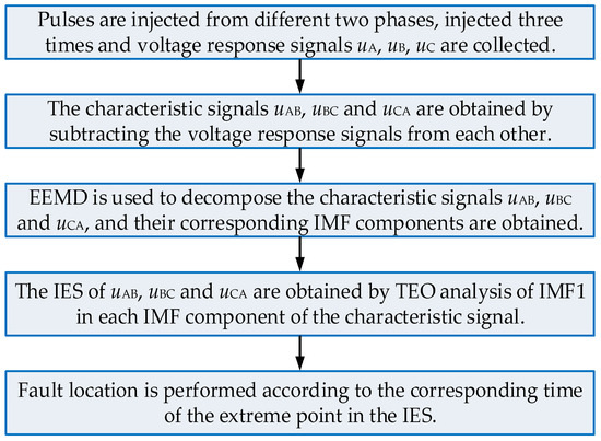
Since TEO only needs three adjacent sample data to obtain the signal source energy at any instant and enables real-time tracking of the waveform variations of the measured signal, which it is suitable for rapid detection and local analysis of the signal [38,39,40]. The high frequency component obtained by EEMD decomposition of the characteristic waveform is IMF1. Because IMF1 is more sensitive to fault information, TEO selects to process IMF1 and obtains its instantaneous energy spectrum (IES). The extreme point in the IES corresponds to the moment when the injection pulse reaches the impedance discontinuity point and returns to the signal acquisition point. Accurate fault location can be realized according to this moment. Figure 11 is the flow chart of fault location using EEMD-TEO.
Figure 11.
Fault location flow chart.
The specific steps of fault location using EEMD-TEO are as follows:
(1) Pulses are injected from two different phases, injected three times, and voltage response signals uA, uB, and uC are collected.
(2) The characteristic signals uAB, uBC, and uCA are obtained by subtracting the voltage response signals from each other.
(3) EEMD is used to decompose the characteristic signals uAB, uBC, and uCA respectively, and their corresponding IMF components are obtained.
(4) The instantaneous energy spectra of uAB, uBC, and uCA are obtained by TEO analysis of IMF1 in each IMF component of the characteristic signal.
(5) Fault location is performed according to the corresponding time of the extreme point in the IES.
3.2. ITSC Fault Location
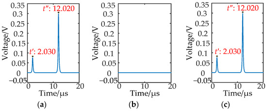
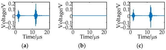
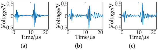
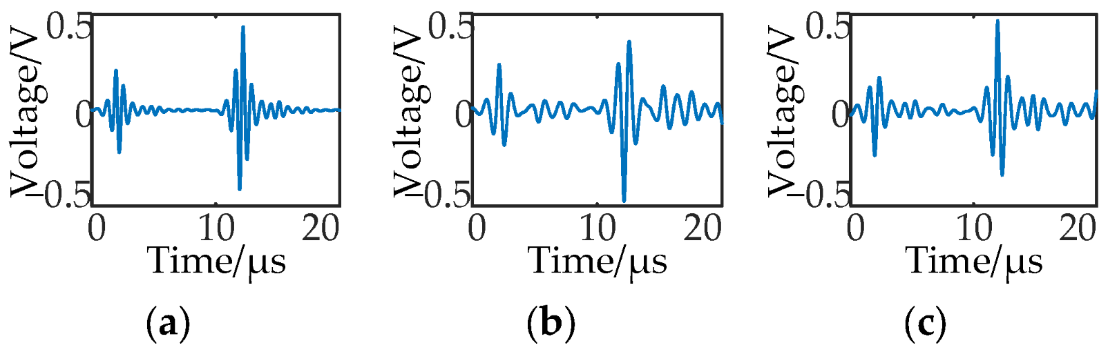
Firstly, the metal ITSC of phase A is set up, and the short circuit point of the near injection side is 200 m, and the short circuit point of the far injection side is 220 m. Then the pulse injection method mentioned above is used to obtain three ITSC characteristic waveforms, and EEMD decomposition is carried out to obtain the IMF1 of the ITSC characteristic waveform shown in Figure 12. The Teager energy value is calculated to obtain the IES of the IMF1 of the ITSC characteristic waveform shown in Figure 13.
Figure 12.
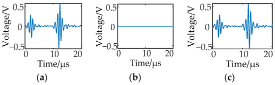
The IMF1 of the characteristic waveform of ITSC: (a) The IMF1 of uAB; (b) The IMF1 of uBC; (c) The IMF1 of uCA.
Figure 13.
IES of IMF1 of ITSC: (a) IES of IMF1 of uAB; (b) IES of IMF1 of uBC; (c) IES of IMF1 of uCA.
Because phase A is the fault phase, the characteristic waveform uBC is a zero line, and the IMF1 and its IES obtained by the corresponding decomposition are also a zero line. The maximum point of the IES obtained by the IMF1s of uAB and uCA is the time when the positive and negative half-cycle square wave pulse of the fault phase reaches the fault point from the winding head end and returns to the winding head end.
Combining Equation (13) with the corresponding time instants of the maximum points in the IES of the characteristic waveforms uAB and uCA, the distances between the fault point and the winding head end can be obtained, respectively. Then, the average value of the two distances calculated from the IES can be taken to reduce the random error.
where l is the distance between the fault point and the winding head end; ν is the traveling wave velocity, and its value is 206.419 m/μs; and are the times taken by the positive and negative half-cycle square wave pulses to reach the fault point from the winding head end and return to the winding head end; and T is the period of the injected square wave pulse, which is 20 μs.
According to Figure 13, the two Teager energy maxima of the IMF1s of the characteristic waveforms uAB and uCA are both 2.030 μs and 12.020 μs at this time. Then the distance between the fault point and the winding head end is 208.999 m.
When the ITSC of phase A occurs and the pulse is injected into phases A and B or phases A and C, there are two fault points in the injection circuit. At this time, due to the influence of multiple catadioptric processes of traveling waves, the fault point is located 208.999 m from the winding head end, which is close to the midpoint of the short circuit point of the near injection side and the short circuit point of the far injection side, 210 m. The results of ITSC fault location under different fault locations and short circuit resistances are shown in Table 3.
Table 3.
ITSC fault location results.
From Table 3, it can be seen that the ITSC fault location result is always close to the midpoint of the short circuit point near the injection side and the short circuit point at the far injection side. The maximum absolute error is 3.058 m, which is not more than 1-turn coil length. Accurate fault location can still be realized when the short circuit resistance is 50 Ω.
3.3. IBSC Fault Location
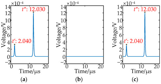
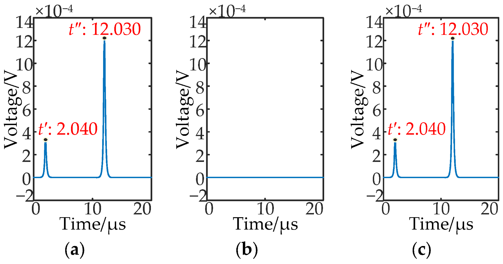
The metallic IBSC occurs in phase A, and the short circuit points of the near injection side and the far injection side are 200 m and 220 m. The IMF1 and its IES of the IBSC characteristic waveform are shown in Figure 14 and Figure 15.
Figure 14.
The IMF1 of the characteristic waveform of IBSC: (a) The IMF1 of uAB; (b) The IMF1 of uBC; (c) The IMF1 of uCA.
Figure 15.
IES of IMF1 of IBSC: (a) IES of IMF1 of uAB; (b) IES of IMF1 of uBC; (c) IES of IMF1 of uCA.
According to Figure 15, it can be seen that the two Teager energy maximum values of the IMF1s of the characteristic waveforms uAB and uCA are 2.040 μs and 12.030 μs. Then, the distance between the fault point and the winding head end at this time can be obtained from Equation (13). It is 210.031 m, and the fault location point is close to the midpoint of the near injection side short circuit point and the far injection side short circuit point, which is the same as that of the ITSC. The results of IBSC fault location under different fault locations and short circuit resistances are shown in Table 4.
Table 4.
IBSC fault location results.
It can be seen from Table 4 that the maximum absolute error of the location result is 4.090 m when the IBSC occurs, which is not more than 1-turn coil length. Accurate fault location can still be realized when the short circuit resistance is 50 Ω.
3.4. IPSC Fault Location
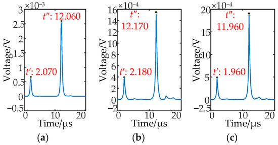
The metal IPSC occurs between phases A and B. The short circuit point of the near injection side is set to 200 m on a branch of phase A, and the short circuit point of the far injection side is set to 220 m on a branch of phase B. The IMF1 and its IES of the IPSC characteristic waveform are shown in Figure 16 and Figure 17, respectively. When the pulses are injected into two different phases, the corresponding time of the maximum point is different. The distance between the fault point and the winding head end can be obtained from Equation (13).
Figure 16.
The IMF1 of the characteristic waveform of IPSC: (a) The IMF1 of uAB; (b) The IMF1 of uBC; (c) The IMF1 of uCA.
Figure 17.
IES of IMF1 of IPSC: (a) IES of IMF1 of uAB; (b) IES of IMF1 of uBC; (c) IES of IMF1 of uCA.
The two Teager energy maximum values of the IMF1s of the characteristic waveforms uAB, uBC, and uCA are 2.070 μs and 12.060 μs, 2.180 μs and 12.170 μs, and 1.960 μs and 11.960 μs. The distance between the fault point and the winding head end under the three injection modes is 213.128 m, 224.481 m, and 202.291 m.
Because phases A and B are the fault phases, when the pulses are injected into phases A and B, there are two fault points in the injection circuit. The traveling wave catadioptric process has a great influence on the fault location so that the fault location is close to the midpoint of the short circuit points of the near injection side and the far injection side. When the pulse is injected into phases A and C or phases B and C, there is only one fault point in the injection circuit. At this time, the traveling wave catadioptric process has little effect on the fault location, and two fault points can be accurately located. The results of IPSC fault location under different fault locations and short circuit resistances are shown in Table 5.
Table 5.
IPSC fault location results.
It can be seen from Table 5 that the maximum absolute errors of the near injection side location results and the far injection side location results are 2.291 m and 8.471 m, respectively, which are not more than 1-turn coil length. Accurate fault location can still be realized when the short circuit resistance is 50 Ω.
3.5. Robustness Analysis of Fault Location Method
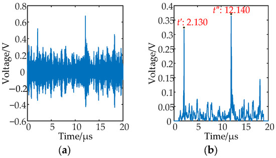
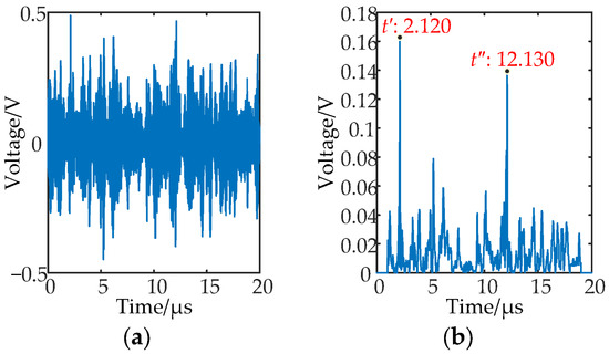
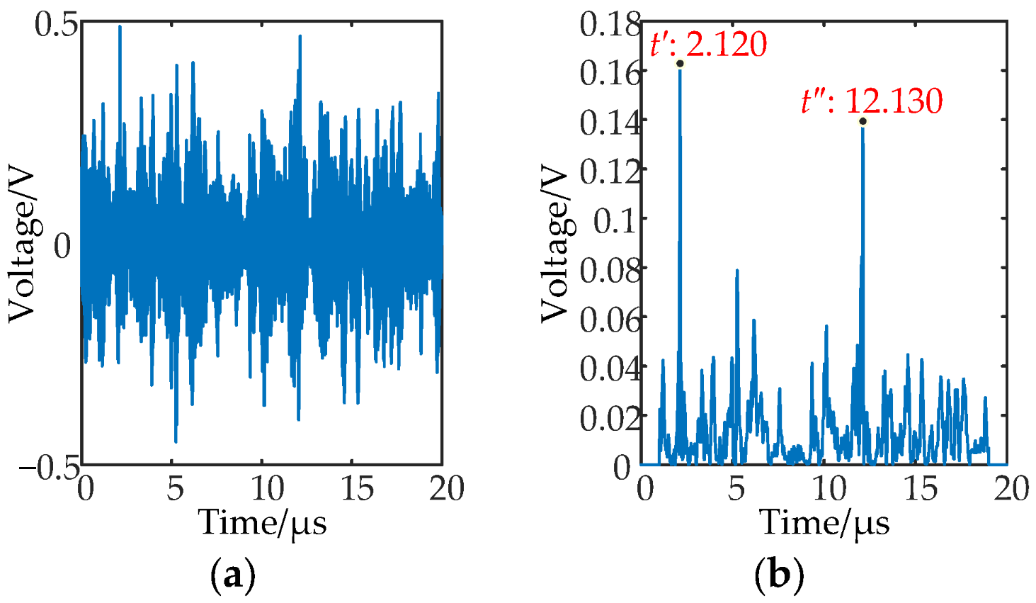
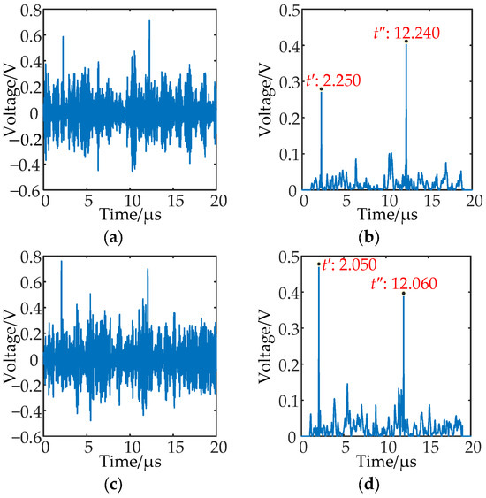
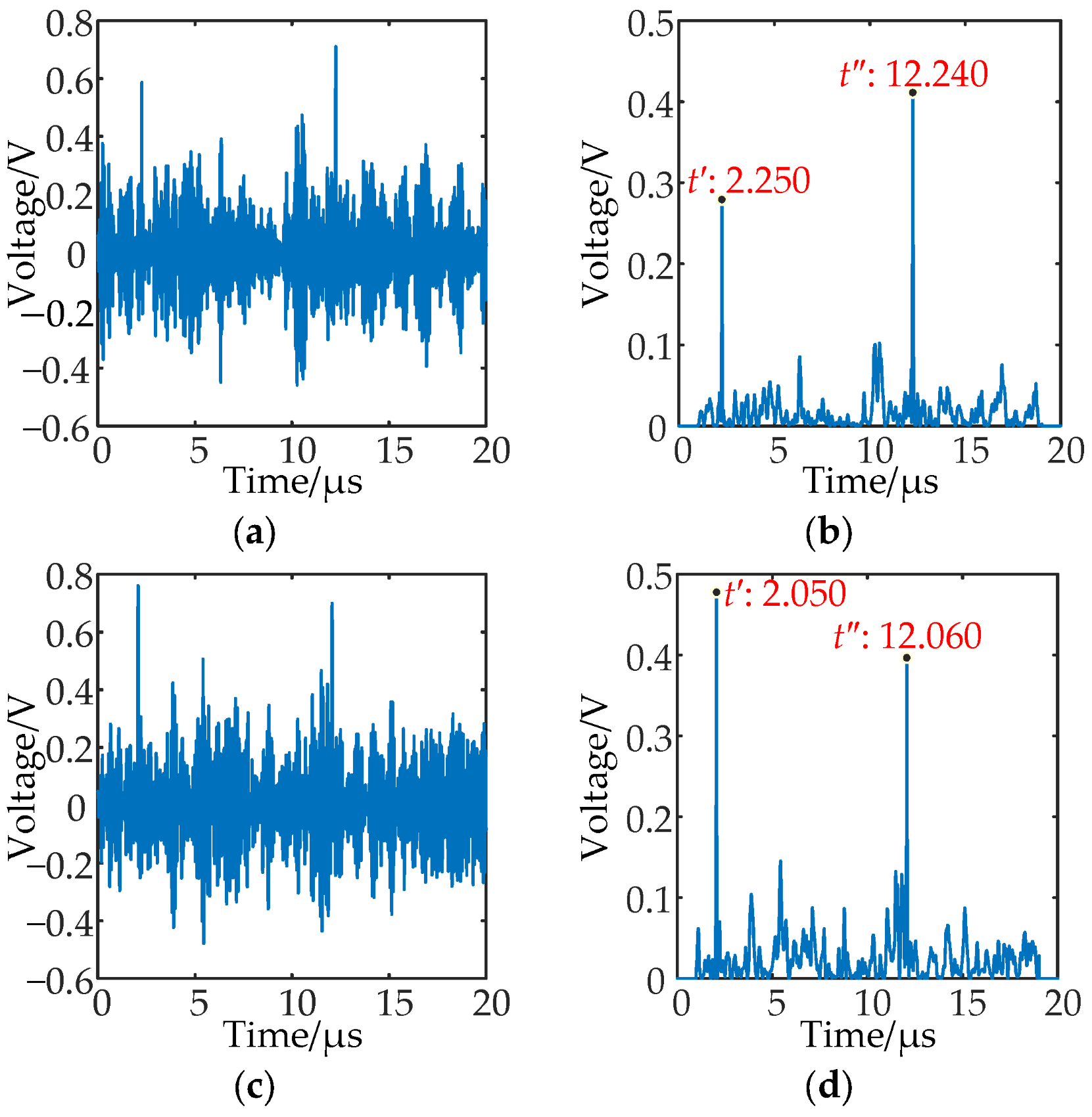
The short circuit point of the near injection side and the short circuit point of the far injection side under the ITSC and the IBSC are set to be 200 m and 220 m from the winding head end of phase A, respectively. Under the IPSC, the short circuit point of the near injection side is 200 m from the winding head end of phase A, and the short circuit point of the far injection side is 220 m from the winding head end of phase B. In order to simulate the real operating conditions of the project site, the short circuit resistance in the above fault scenarios is set to 50 Ω; the Gaussian white noise with a signal-to-noise ratio of 20 dB is superimposed on the voltage response waveform to simulate the background noise of the field acquisition equipment, and the time offset of +10 sampling points is superimposed to simulate the acquisition error caused by the trigger lag of the acquisition system. At the same time, in the simulation model, the random deviation of +15% is added to the unit length inductance and ground capacitance of the rotor winding to simulate the parameter dispersion characteristics caused by winding processing and installation tolerance, long-term operation insulation aging, and vibration deformation. The ITSC and the IBSC select the IES of the IMF1 of the characteristic waveform uAB for fault location, as shown in Figure 18 and Figure 19. The IES of the IMF1 of the characteristic waveforms uBC and uCA is selected for fault location, as shown in Figure 20.
Figure 18.
The location result of ITSC under multiple compound interferences: (a) The IMF1 of uAB; (b) IES of IMF1 of uAB.
Figure 19.
The location result of IBSC under multiple compound interferences: (a) The IMF1 of uAB; (b) IES of IMF1 of uAB.
Figure 20.
The location result of IPSC under multiple compound interferences: (a) The IMF1 of uBC; (b) IES of IMF1 of uBC; (c) The IMF1 of uCA; (d) IES of IMF1 of uCA.
The fault location can be obtained by substituting the corresponding time of the maximum point in the figures into Equation (13). The location results of ITSC and IBSC under multiple compound interferences are 220.352 m and 219.320 m, and the location errors are 10.352 m and 9.320 m. The location results of the IPSC are 231.705 m and 212.096 m, and the location errors are 11.705 m and 12.096 m. Although the fault location error under multiple compound interference is increased compared with that without interference, the location error is still less than the length of the 2-turn coil, and the location results are close to the fault region.
In summary, the fault location method proposed in this paper can still accurately locate the fault location under multiple compound interferences and has excellent anti-interference ability, strong robustness, and good engineering applicability.
4. Short Circuit Fault Severity Discrimination
The longer the length of the short circuited winding (hereinafter referred to as the fault length) of the RWSC fault, the higher the short circuited potential and the greater the impact on the generator. Therefore, the fault length is usually regarded as the criterion for judging the severity of the short circuit fault. For IPSC, the fault location method described above can locate the near injection side short circuit point and the far injection side short circuit point, and then the fault length can be obtained. For ITSC or IBSC, only the midpoint of the short circuit point near the injection side and the short circuit point at the far injection side can be located. In order to obtain the specific location of the two short circuit points at this time, it is necessary to judge the severity of the short circuit fault to obtain the fault length.
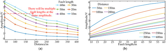
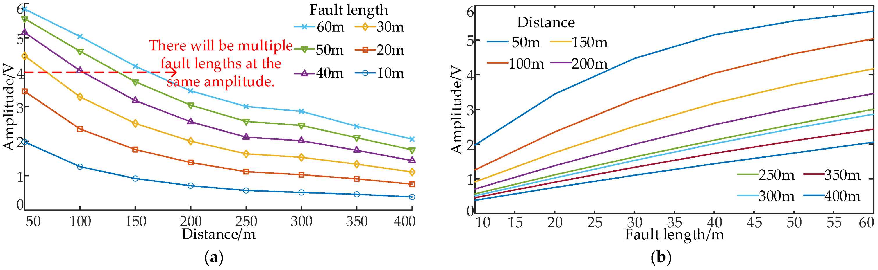
The rotor winding of an adjustable speed hydro-generating unit can be regarded as a lossy transmission line; the traveling wave must be accompanied by attenuation and deformation during the transmission process, which leads to a certain degree of distortion of the characteristic waveform. When the ITSC or IBSC occurs in phase A of the rotor winding, the pulse is injected into two different phases, and the distance from the fault point to the winding head end and the fault length are changed to obtain the variation curve of the characteristic waveform amplitude with these two factors. Because the fault phase is the A phase, when the pulse is injected into phases B and C, the characteristic waveform is a zero line. When the pulse is injected into phases A and C or phases A and B, the amplitude of the characteristic waveform is the same. Therefore, only the curve of the amplitude with the distance from the fault point to the winding head end and the curve of the amplitude with the fault length are given when the pulse is injected into phases A and B, as shown in Figure 21.
Figure 21.
Amplitude change curve: (a) Curve of amplitude changing with fault location; (b) Curve of amplitude changing with fault length.
It can be observed that the amplitude of the characteristic waveform decreases as the distance from the fault point to the winding head end increases, following an exponential decay pattern. When the fault location is the same, the longer the fault length, the larger the amplitude of the characteristic waveform. When the amplitude is used as the evaluation criterion of fault severity, it is greatly affected by the distance from the fault point to the winding head end. Under the same amplitude, there may be multiple fault lengths, which cannot effectively distinguish the severity of the fault.
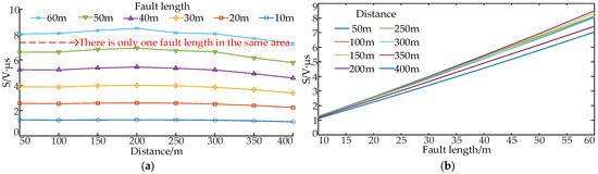
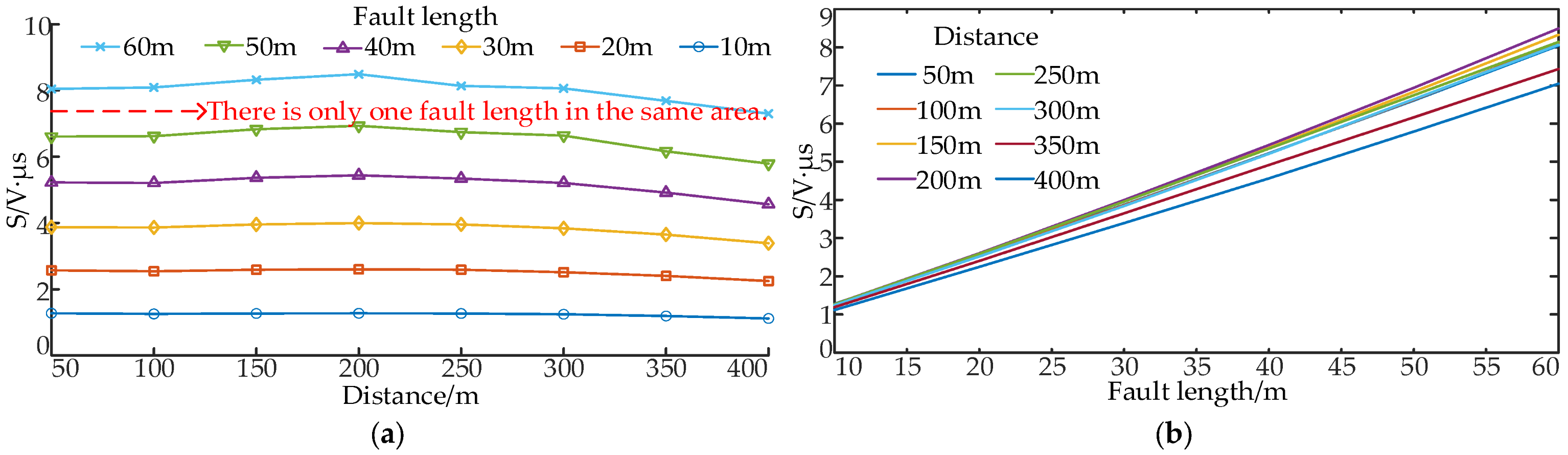
To eliminate the influence of the distance from the fault point to the winding head end on the severity of the fault, this paper uses the area S in Equation (4) as the fault factor to describe the severity of the fault. When the ITSC occurs, the pulse is injected into phases A and B, and the area changes with the distance from the fault point to the winding head end, and the area changes with the fault length, as shown in Figure 22.
Figure 22.
Area change curve: (a) Curve of area changing with fault location; (b) Curve of area changing with fault length.
Compared with the method of measuring the severity of the fault with the amplitude of the characteristic waveform, it is more stable to use the area as the fault factor to judge the severity of the fault. It is not affected by the distance from the fault point to the winding head end, and only one fault length will appear under the same area. This area has a strong linear positive correlation with the fault length. The longer the fault length, the greater the number of fault turns, the larger the fault area, and the more severe the fault. After calculation, the linear correlation coefficients under different fault lengths are all greater than 0.990. Therefore, it can be used as a fault factor to measure the severity of the fault more effectively. It should be noted that the fault location method proposed in this paper only needs to obtain the propagation wave velocity of the injected pulse in the rotor winding of the adjustable speed hydro-generating unit in advance to determine the fault location. Combined with the determined fault location and the calculated fault factor, the fault length can be accurately converted according to the relationship between the fault factor and the fault length, so as to realize the quantitative evaluation of the fault severity. In summary, the method proposed in this paper does not need to rely on the exclusive design data of the unit and can be adapted to different types and different parameters of the adjustable speed hydro-generator units.
5. Conclusions
In this paper, a new offline diagnosis method for the internal RWSC of an adjustable speed hydro-generating unit is proposed. The main conclusions are as follows.
(1) The internal RWSC fault type and fault phase identification method are proposed. The characteristic waveforms of the internal RWSC of an adjustable speed hydro-generating unit are analyzed, and the fault characteristics under different short circuit faults are summarized. A fault-type identification method based on detecting the reverse polarity sub-spike is proposed. The minimum fault identification sensitivity of the identification method under the remote high resistance fault is 2.188, which can effectively and accurately distinguish the fault phase and fault type.
(2) A method of combining EEMD and TEO is proposed for fault location. The results show that for the ITSC and IBSC, the midpoint of the near injection side short circuit point and the far injection side short circuit point can be located. For IPSC, both the near injection side short circuit point and the far injection side short circuit point can be located. The location error under various short circuit types does not exceed the length of the 1-turn coil of the rotor winding. Although the location error of this method under multiple compound interferences increases slightly, it can still accurately locate the fault location under various fault types, and the location error does not exceed the length of the 2-turn coil of the rotor winding, which has strong robustness.
(3) Aiming at ITSC and IBSC faults, a fault factor is proposed to measure the severity of the fault by using the characteristic waveform of the fault phase and the area enclosed by the zero line. The results show that the method can eliminate the influence of the distance from the fault point to the winding head end on the fault severity discrimination, and the linear correlation coefficients under different fault lengths are all greater than 0.990, which has higher reliability and meets the engineering needs.
Although the method proposed in this paper can realize the accurate diagnosis and location of the internal RWSC of the large-capacity adjustable speed hydrogenerator unit, the ANSYS Maxwell high-precision simulation model based on the real parameters of the unit can fully verify the effectiveness of the method. However, the field experiment of the unit needs destructive transformation of the winding, which will cause irreversible damage to the equipment and have safety risks. The bench experiment is limited by the high cost and long cycle of the customized winding, so the field and bench entity experiments have not been carried out. In the future, the author will actively promote the construction of the experimental bench and the experimental test of the field unit and combine the measured data to optimize the performance of the method and improve the engineering adaptability.
Author Contributions
Conceptualization, J.Q. and K.W.; methodology, J.Q. and K.W.; software, K.W. and Y.W.; validation, J.Q., K.W. and Y.W.; formal analysis, Q.L., X.Y. (Xin Yin) and W.J.; investigation, W.J. and X.Y. (Xianggen Yin); resources, Y.W. and X.Y. (Xin Yin); data curation, Q.L. and X.Y. (Xianggen Yin); writing—original draft preparation, J.Q. and K.W.; writing—review and editing, J.Q. and K.W.; visualization, Q.L., X.Y. (Xin Yin), W.J., and X.Y. (Xianggen Yin); supervision, Q.L., X.Y. (Xin Yin), W.J., and X.Y. (Xianggen Yin); project administration, J.Q. and Y.W.; funding acquisition, J.Q. All authors have read and agreed to the published version of the manuscript.
Funding
This research was funded by the National Natural Science Foundation of China, grant number 52507099, and the Science Research Project of Hebei Education Department, grant number BJ2026149.
Institutional Review Board Statement
Not applicable.
Informed Consent Statement
Not applicable.
Data Availability Statement
The original contributions presented in the study are included in the article, further inquiries can be directed to the corresponding author.
Conflicts of Interest
Author Qinghui Lu was employed by the Jinan Power Supply Company, State Grid Shandong Electric Power Company. The remaining authors declare that the research was conducted in the absence of any commercial or financial relationships that could be construed as a potential conflict of interest.
Appendix A
Table A1.
Nomenclature of symbols.
References
- Li, Y.; Song, F.; Guo, W. Transient Characteristics and Operation Regulation of Grid-Connected Variable Speed Pumped Storage-Wind-Solar Hybrid Power System. Energy Sci. Eng. 2024, 13, 416–433. [Google Scholar] [CrossRef] [Scilit]
- Chen, Y.H.; Xu, W.; Liu, Y.; Bao, Z.; Mao, Z.X.; Rashad, E.M. Modeling and Transient Response Analysis of Doubly-Fed Variable Speed Pumped Storage Unit in Pumping Mode. IEEE Trans. Ind. Electron. 2023, 70, 9935–9947. [Google Scholar] [CrossRef] [Scilit]
- Deng, Y.W.; Wang, P.F.; Morabito, A.; Feng, W.F.; Mahmud, A.; Chen, D.Y.; Hendrick, P. Dynamic Analysis of Variable-Speed Pumped Storage Plants for Mitigating Effects of Excess Wind Power Generation. Int. J. Electr. Power Energy Syst. 2022, 135, 107453. [Google Scholar] [CrossRef] [Scilit]
- Chen, Y.H.; Xu, W.; Liu, Y.; Rashad, E.M.; Bao, Z.; Jiang, J.C.; Mao, Z.X. Reduced-Order System Frequency Response Modeling for the Power Grid Integrated With the Type-II Doubly-Fed Variable Speed Pumped Storage Units. IEEE Trans. Power Electron. 2022, 37, 10994–11006. [Google Scholar] [CrossRef] [Scilit]
- Hu, J.; Tao, D.; Sun, Y. Analysis of Operating Characteristics of Variable Speed Pumped Storage Motor-Generator. IEEE Access 2023, 11, 52117–52128. [Google Scholar] [CrossRef] [Scilit]
- Bai, J.; Gui, L.; Li, R. Multi-Loop Model Based Internal Fault Analysis of Variable Speed Pumped Hydro Machines. IEEE Trans. Energy Convers. 2025, 39, 2728–2741. [Google Scholar] [CrossRef] [Scilit]
- Alam, M.; Payami, S. Diagnosis of Interturn Short-Circuits in SRMs by High-Frequency Switching of Phases Amid Low-Torque Unaligned Rotor Positions. IEEE Trans. Ind. Electron. 2023, 70, 7537–7546. [Google Scholar]
- Doorwar, A.; Bhalja, B.R.; Malik, O.P. Novel Approach for Synchronous Generator Protection Using New Differential Component. IEEE Trans. Energy Convers. 2023, 38, 180–191. [Google Scholar] [CrossRef] [Scilit]
- Li, J.; Niu, H.; Zhu, Y.; Xing, K.; Gui, L. Main Protection for Rotor Windings of Large AC Excitation Variable-Speed Pumped Storage Units Optimized Design. Hydropower Pumped Storage 2025, 11, 59–64. [Google Scholar]
- Bai, J.; Gui, L.; Liu, M.; Li, Y.; Gao, C.; Cao, T.; Yan, Y. Performance Analysis of New Main Protection Scheme for Rotor Winding of Variable Speed Pumped Storage Units. Electr. Power 2024, 57, 208–217. [Google Scholar]
- Aziz, M.S.; Zhang, J.Z.; Ruzimov, S.; Huang, X. Detection and Localization of Rotor Winding Inter-Turn Short Circuit Fault in DFIG Using Zero-Sequence Current Component Under Variable Operating Conditions. Sensors 2025, 25, 2815. [Google Scholar] [CrossRef] [Scilit] [PubMed]
- Ma, C.W.; Zhang, B.J.; Song, W.S.; Jia, Z.; Huang, W.Q.; Huang, J.C. A Stationary-Frame Residual-Current-Based ITSC Localization Method for Induction Motors Considering Effect of Different Faulty Phase. IEEE J. Emerg. Sel. Top. Power Electron. 2025, 13, 1710–1720. [Google Scholar] [CrossRef] [Scilit]
- Sun, H.; Liu, C.; Fu, Y. Application of detection technology based on traveling wave theory in rotor winding fault diagnosis. Electr. Eng. 2022, 43–45+50. [Google Scholar] [CrossRef]
- Jin, Y.S.; Wu, H.; Zheng, J.F.; Zhang, J.; Liu, Z. Power Transformer Fault Diagnosis Based on Improved BP Neural Network. Electronics 2023, 12, 3526. [Google Scholar] [CrossRef] [Scilit]
- Khoshbakht, S.; Moosavi, S.M.; Cruz, S.M.A. Hybrid CNN-Transformer Approach for Rotor Interturn Short-Circuit Fault Detection in Doubly Fed Induction Generators at Synchronous Speed. IET Electr. Power Appl. 2025, 19, e70123. [Google Scholar] [CrossRef] [Scilit]
- Battulga, B.; Shaikh, M.F.; Lee, S.B.; Osama, M. Inverter-Embedded Detection of Rotor Winding Faults in Doubly Fed Induction Generators for Wind Energy Applications. IEEE Trans. Energy Convers. 2023, 38, 646–652. [Google Scholar] [CrossRef] [Scilit]
- Senobari, R.K.; Kakolaki, S.E.H.; Sadeh, J. Comprehensive experimental study on a wound-rotor asynchronous machine fault detection through frequency response analysis. Int. J. Electr. Power Energy Syst. 2025, 170, 110852. [Google Scholar] [CrossRef] [Scilit]
- Lu, Q.; Yin, X.; Qiao, J. Short circuit fault identification and diagnosis analysis of rotor winding for variable speed pumped storage unit. Energy Rep. 2022, 8, 34–43. [Google Scholar] [CrossRef] [Scilit]
- Wang, D.; Yu, D.; Gao, H. Frequency Modification Algorithm-Based Traveling Wave Fault Location Approach for Overhead Transmission Lines with Structural Changes. Prot. Control Mod. Power Syst. 2025, 10, 1–12. [Google Scholar] [CrossRef] [Scilit]
- Shu, H.; Liu, H.; Tang, Y. Fault Identification Method for Measured Travelling Wave of Transmission Line Based on CSCRFAM-Transformer. Prot. Control Mod. Power Syst. 2025, 10, 69–82. [Google Scholar] [CrossRef] [Scilit]
- Luo, J.; Liu, Y.; Cui, Q. Single-ended Time Domain Fault Location Based on Transient Signal Measurements of Transmission Lines. Prot. Control Mod. Power Syst. 2024, 9, 61–74. [Google Scholar] [CrossRef] [Scilit]
- Chen, Y.B.; Cui, H.S.; Huang, C.W.; Hsu, W.T. Improving Transmission Line Fault Diagnosis Based on EEMD and Power Spectral Entropy. Entropy 2024, 26, 806. [Google Scholar] [CrossRef] [Scilit] [PubMed]
- Zhou, F.; Sun, Q.; Wang, Y.; Wang, W. A Fault Diagnosis Method Based on the Transmission Characteristics of Bearing Vibration in Multi-Axis Systems. Electr. Eng. 2025, 107, 14915–14933. [Google Scholar] [CrossRef] [Scilit]
- Tang, T.; Li, X.; Zeng, X.; Zhou, Y.; Yuan, K.; Bi, L. Accurate Detection Method of Traveling Wave Shape Based on EEMD and L1 Norm Regularization. Int. J. Electr. Power Energy Syst. 2024, 159, 110008. [Google Scholar] [CrossRef] [Scilit]
- Wang, Y.; Xie, L.; Liu, F.; Yu, K.; Zeng, X.; Bi, L.; Tang, X. Fault Location Method for Distribution Network Considering Distortion of Traveling Wavefronts. Int. J. Electr. Power Energy Syst. 2024, 159, 110065. [Google Scholar] [CrossRef] [Scilit]
- Sarangi, S.; Biswal, C.; Sahu, B.K.; Samanta, I.S.; Rout, P.K. Fault Detection Technique Using Time-Varying Filter-EMD and Differential-CUSUM for LVDC Microgrid System. Electr. Power Syst. Res. 2023, 219, 109254. [Google Scholar] [CrossRef] [Scilit]
- Sarangi, S.; Sahu, B.K.; Rout, P.K. High-Impedance Fault Identification and Location by Using Mode Decomposition Integrated Adaptive Multi-Kernel Extreme Learning Machine Technique for Distributed Generator-Based Microgrid. Electr. Eng. 2023, 105, 383–406. [Google Scholar] [CrossRef] [Scilit]
- Zhang, M.G.; Zhao, W.Y.; Li, P.C. Two-Terminal Fault Combination Location Method on MMC-HVDC Transmission Lines Based on Ensemble Empirical Mode Decomposition. Energy Rep. 2023, 9, 987–995. [Google Scholar] [CrossRef] [Scilit]
- Zhang, Z.Y.; Cao, W.H.; Hu, W.K. An Improved EEMD-GCC Method for Pipeline Leak Detection and Localization with Maglev Vibration Detector. Measurement 2025, 252, 117244. [Google Scholar] [CrossRef] [Scilit]
- Xie, L.; Luo, L.; Ma, J.; Li, Y.; Zhang, M.; Zeng, X.; Cao, Y. A Novel Fault Location Method for Hybrid Lines Based on Traveling Wave. Int. J. Electr. Power Energy Syst. 2022, 141, 108102. [Google Scholar] [CrossRef] [Scilit]
- Babak, V.; Babak, S.; Zaporozhets, A. Statistical Assessment of Diagnostic Parameters. In Statistical Diagnostics of Electric Power Equipment; Springer: Cham, Switzerland, 2025; Volume 573, pp. 145–179. [Google Scholar]
- Bebars, A.D.; Eladl, A.A.; Abdulsalam, G.M.; Badran, E.A. Internal Electrical Fault Detection Techniques in DFIG-Based Wind Turbines: A Review. Prot. Control Mod. Power Syst. 2022, 7, 18. [Google Scholar] [CrossRef] [Scilit]
- Jiang, W.L.; Murray, S.K.; Zaman, M.S.; De Vleeschouwer, H.; Moens, P.; Roig, J.; Trescases, O. An Integrated GaN Overcurrent Protection Circuit for Power HEMTs Using SenseHEMT. IEEE Trans. Power Electron. 2022, 37, 9314–9324. [Google Scholar] [CrossRef] [Scilit]
- Liu, F.; Xie, L.; Yu, K.; Wang, Y.; Zeng, X.; Bi, L.; Liu, F.; Tang, X. A Novel Fault Location Method Based on Traveling Wave for Multi-Branch Distribution Network. Electr. Power Syst. Res. 2023, 224, 109753. [Google Scholar] [CrossRef] [Scilit]
- Wan, W.L.; Qin, Z.; Deng, M.G.; Liu, Y. A New Traveling Wave Location Method for Wide Area Power Grid Based on Fault Line Trust Region and Second Path Traveling Wave. Electr. Power Syst. Res. 2025, 245, 111581. [Google Scholar] [CrossRef] [Scilit]
- Yu, D.C.; Zhou, N.C.; Liao, J.Q.; Wang, Q.G.; Lyu, Y.Z. Modified VMD Algorithm-Based Fault Location Method for Overhead-Cable Hybrid Transmission Line in MTDC System. IEEE Trans. Instrum. Meas. 2024, 73, 3517711. [Google Scholar] [CrossRef] [Scilit]
- Zeng, R.C.; Zhang, L.L.; Wu, Q.H. Fault Location Scheme for Multi-Terminal Transmission Line Based on Frequency-Dependent Traveling Wave Velocity and Distance Matrix. IEEE Trans. Power Deliv. 2023, 38, 3980–3990. [Google Scholar] [CrossRef] [Scilit]
- Liu, Z.J.; Li, D.Y.; Liu, H.W.; Dai, J.; Li, P.C.; Zhang, C.L.; Feng, F.; Li, M. A Fault Traveling Wave Localization Method for Distribution Networks Based on Improved Wavelet Threshold Denoising and ICEEMDAN-TEO. Energy Rep. 2026, 15, 109116. [Google Scholar] [CrossRef] [Scilit]
- Cao, J.Y.; Wang, Y.W.; Wu, L.J.; Zhao, Y.M.; Wang, L. A Single-End Location Method for Small Current Grounding System Based on the Minimum Comprehensive Entropy Kurtosis Ratio and Morphological Gradient. Appl. Sci. 2025, 15, 3539. [Google Scholar] [CrossRef] [Scilit]
- Zeng, R.C.; Wu, Q.H.; Zhang, L.L. Two-Terminal Traveling Wave Fault Location Based on Successive Variational Mode Decomposition and Frequency-Dependent Propagation Velocity. Electr. Power Syst. Res. 2022, 213, 108768. [Google Scholar] [CrossRef] [Scilit]

Disclaimer/Publisher’s Note: The statements, opinions and data contained in all publications are solely those of the individual author(s) and contributor(s) and not of MDPI and/or the editor(s). MDPI and/or the editor(s) disclaim responsibility for any injury to people or property resulting from any ideas, methods, instructions or products referred to in the content. |
© 2026 by the authors. Licensee MDPI, Basel, Switzerland. This article is an open access article distributed under the terms and conditions of the Creative Commons Attribution (CC BY) license.