DDR-PINN: A Dynamic Domain–Gradient Reweighting Physics-Informed Neural Network

Abstract

Physics-informed neural networks (PINNs) solve partial differential equations (PDEs) by embedding physical conditions as soft penalties into the loss function. However, the coexistence of multiple loss components often leads to gradient conflicts, degrading convergence and solution accuracy. To address this issue, we propose a dynamic domain–gradient loss reweighting PINN (DDR-PINN). The proposed method introduces a dual-residual reweighting mechanism based on gradient variations, where adaptive weights are derived from the L2 norm of the dot product between loss gradients and residuals. These weights are further normalized through a nonlinear hyperbolic tangent transformation, enabling dynamic and balanced reweighting of interior, initial, and boundary domain losses throughout training. Extensive numerical experiments on PDEs with both Dirichlet and Neumann boundary conditions demonstrate that the DDR-PINN consistently outperforms the standard PINN, APINN, and VI-PINN with the fewest trainable parameters.

1. Introduction

In recent years, machine learning (ML) has achieved remarkable advancements, driven by rapid growth in data availability and computational power. As a representative data-driven approach, traditional ML technology extracts knowledge from massive datasets. However, its effectiveness is often constrained by the availability of high-quality labeled data and the limited interpretability of model mechanisms [1,2]. In contrast, physics-driven approaches rely on explicit governing equations and expert knowledge [3], which frequently lead to complex modeling processes and limited generalization performance. Therefore, the concept of physics-informed machine learning (PIML) has emerged as a promising framework that embeds prior physical knowledge into ML models, enabling accurate solutions for physical problems under limited or even data-free conditions [4,5]. Physics-Informed Neural Networks (PINNs) constitute a key research direction within PIML [6]. By incorporating partial differential equations (PDEs), boundary and initial conditions into the loss function, PINNs leverage automatic differentiation to approximate PDE solutions [7,8]. Owing to their mesh-free nature and flexibility, nowadays, PINNs have been successfully applied across a wide range of scientific and engineering fields, including materials science [9], mechanics [10,11], energy [12,13], and related fields [14,15,16].

Despite these advantages, PINNs continue to face several critical challenges, including high computational complexity, slow convergence, and limited training stability [17,18]. These issues primarily arise from the composite structure of the PINN loss function, which simultaneously incorporates interior PDE and boundary condition residuals. Training discrepancies in scale and numerical characteristics often lead to conflicting gradients and oscillatory convergence [19]. To address these challenges, researchers have conducted extensive efforts. Focused on critical regions or physical conditions, adjusting sampling or training strategies makes PINNs more effective. The DP-PINN+ [20] is a novel training framework for PINNs, which divides the training process into two phases based on specific time points. The DSAIS-PINN [21] makes PINNs focus on high-loss regions based on dynamic seed importance sampling. Meanwhile, architecture improvements can fully utilize the inherent potential of PINNs to strengthen the overall solving capability. The Deeper-PINN [22] alleviates the pathologies of PINN initialization by mapping features into a high-dimensional space with element multiplication. Causal PINNs [23] incorporate ResNet blocks into the architecture for mapping identity into residuals, making PINNs consistent with physical causal constraints. Furthermore, the loss function optimization can more directly mitigate conflicts and convergence challenges. The S-PINN [24] introduces a new loss function based on residuals of conserved quantities to alleviate conflicts in multi-layer co-optimization. VI-PINNs [25] output mean and variance, and incorporate the modified negative log-likelihood loss to achieve fast training. As discussed above, although PINN studies related to strategy adjustment and architectural optimization have achieved notable progress, they fail to fundamentally resolve the conflict among loss components, and convergence issues still exist in PDEs with complex boundary conditions or source terms.

To further alleviate convergence conflicts, extensive work has been developed on loss weight adjustment. The APINN [26] dynamically adjusts weights based on multi-task learning tasks. AdaPW [27] focuses on high-error sampling points by updating the weight distribution of PDE residuals and training status. BRDR-Weighting PINNs [28] balance residuals and learning rates to scale the original loss. The FPINN [29] computes Caputo fractional derivatives and outputs numerical solutions. The GVW-PINN [30] adaptively tunes weights based on the variance of gradients, which is constrained by the two-stage training strategy. The IPD-PINN adopts partial derivatives as branch neural networks for convergence guidance but raises model complexity [31]. Above all, the weight adjustment of PINNs is mainly focused on residuals and learning efficiency. However, the PINNs are the approximate approaches to the exact solutions for PDEs, and errors exist inevitably. Thus, the PINN should focus on regions with a high residual change rate, and those with large residuals. Importantly, though raising accuracy, most weight-adjusted PINN methods introduce additional hyperparameters, which complicate the modeling process.

To address these issues, we propose a dynamic domain reweighting-guided PINN (DDR-PINN) based on fusing gradients and residuals, aiming to alleviate potential conflicts between loss terms and accelerate the convergence of PINNs. Unlike existing adaptive PINNs focused on the residuals of the solution function, we guide PINNs via the gradient, which directly affects the partial derivatives in PDEs and shortens the error propagation path. The gradients and residuals are combined into the loss function to guide the PINN to converge towards regions with high variation intensity and large residuals. The main contributions of this paper are summarized as follows:

• We propose a reweighting PINN without additional hyperparameters and trainable parameters, which alleviates loss term conflicts among the interior, initial, and boundary domains, achieving superior convergence stability and accuracy for PDE solving.
• We design different loss functions for Dirichlet and Neumann boundary conditions, to distinguish between derivative loss and solution loss, extending the applicability of the DDR-PINN across diverse application scenarios.
• We conduct comprehensive experiments on different PDEs, including 1D, 2D and 3D cases. The results show that the proposed DDR-PINN achieves the highest accuracy compared with the standard PINN, APINN, and VI-PINN with the fewest trainable parameters.

The structure of this paper is organized as follows: Section 2 introduces the relevant concepts of PDEs and the standard PINN. In Section 3, we describe the proposed DDR-PINN and its loss function. Section 4 details the experimental setup and compares the results of different PINNs in six inhomogeneous PDEs. In Section 4 and Section 5, we discuss and summarize the main conclusions.

2. Related Work

2.1. Partial Differential Equations

The general form of the PDE is mathematically formulated as follows:

$$\left\{\begin{array}{l}\mathcal{H}\left(u\left(X,t\right)\right)=f\left(X,t\right),X\mathrm{ϵ}\mathrm{\Omega },tϵ\left(t_0,\infty \right)\hfill \\ \mathcal{B}\left(u\left(X,t\right)\right)=g\left(X,t\right),X\mathrm{ϵ}\partial \mathrm{\Omega },tϵ\left(t_0,\infty \right)\hfill \\ \mathcal{T}\left(u\left(X,t\right)\right)=h\left(X,t\right),X\mathrm{ϵ}\mathrm{\Omega },{t=t}_0\hfill \end{array}\right.,$$

(1)

where $X={\left(x,y,\cdots ,z\right)}^T\in \Omega$ denotes the space coordinate point, and $\mathrm{\Omega }$ is a bounded domain in ${ℝ}^N$ with boundary $\mathrm{\partial }\Omega$, $t$ denotes the time point, and $t_0$ is the initial time. $\mathcal{H}$, $\mathcal{B}$ and $\mathcal{T}$ are differential operators in the interior, boundary and initial domains, $u\left(X,t\right)$ is the unknown solution function of the PDE, $f\left(X,t\right)$, $g\left(X,t\right)$ and $h\left(X,t\right)$ are known functions. The inhomogeneous PDE refers to $f\left(X,t\right)$ characterized by a nonzero source term, corresponding to the source term of the physical problems. Furthermore, the initial condition can be regarded as a special type of boundary condition, and the boundary conditions are imposed to ensure the uniqueness of the solution to the PDE.

2.2. Physics-Informed Neural Networks

The architecture of the standard PINN is based on a multi-layer perceptron (MLP), which takes spatiotemporal coordinates as input. And $\widehat{u}$ denotes the output solution value of the PINN.

$${\mathcal{L}}_r={\displaystyle \frac{1}{N_r}}{\displaystyle \sum _{k=1}^{N_r}{\left[\mathcal{H}\left({\widehat{u}}_k\right)-f\left(X_k,t_k\right)\right]}^2},$$

(2)

$${\mathcal{L}}_b={\displaystyle \frac{1}{N_b}}{\displaystyle \sum _{k=1}^{N_b}{\left[\mathcal{B}\left({\widehat{u}}_k\right)-g\left(X_k,t_k\right)\right]}^2},$$

(3)

$${\mathcal{L}}_i={\displaystyle \frac{1}{N_i}}{\displaystyle \sum _{k=1}^{N_i}{\left[\mathcal{T}\left({\widehat{u}}_k\right)-h\left(X_k,t_0\right)\right]}^2},$$

(4)

$${\mathcal{L}}_t={\mathcal{L}}_r+{\mathcal{L}}_b+{\mathcal{L}}_i+{\mathcal{L}}_o,$$

(5)

where ${\mathcal{L}}_r$, ${\mathcal{L}}_b$ and ${\mathcal{L}}_i$ are loss terms in the interior, boundary and initial domain, and ${\mathcal{L}}_t$ is the total loss of PINNs. ${\mathcal{L}}_o$ denotes the additional loss, including the data loss if the observational data are available, and the additional boundary-derivative loss in the Neumann boundary condition.

3. Methodology

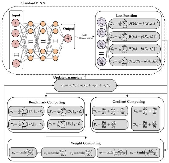
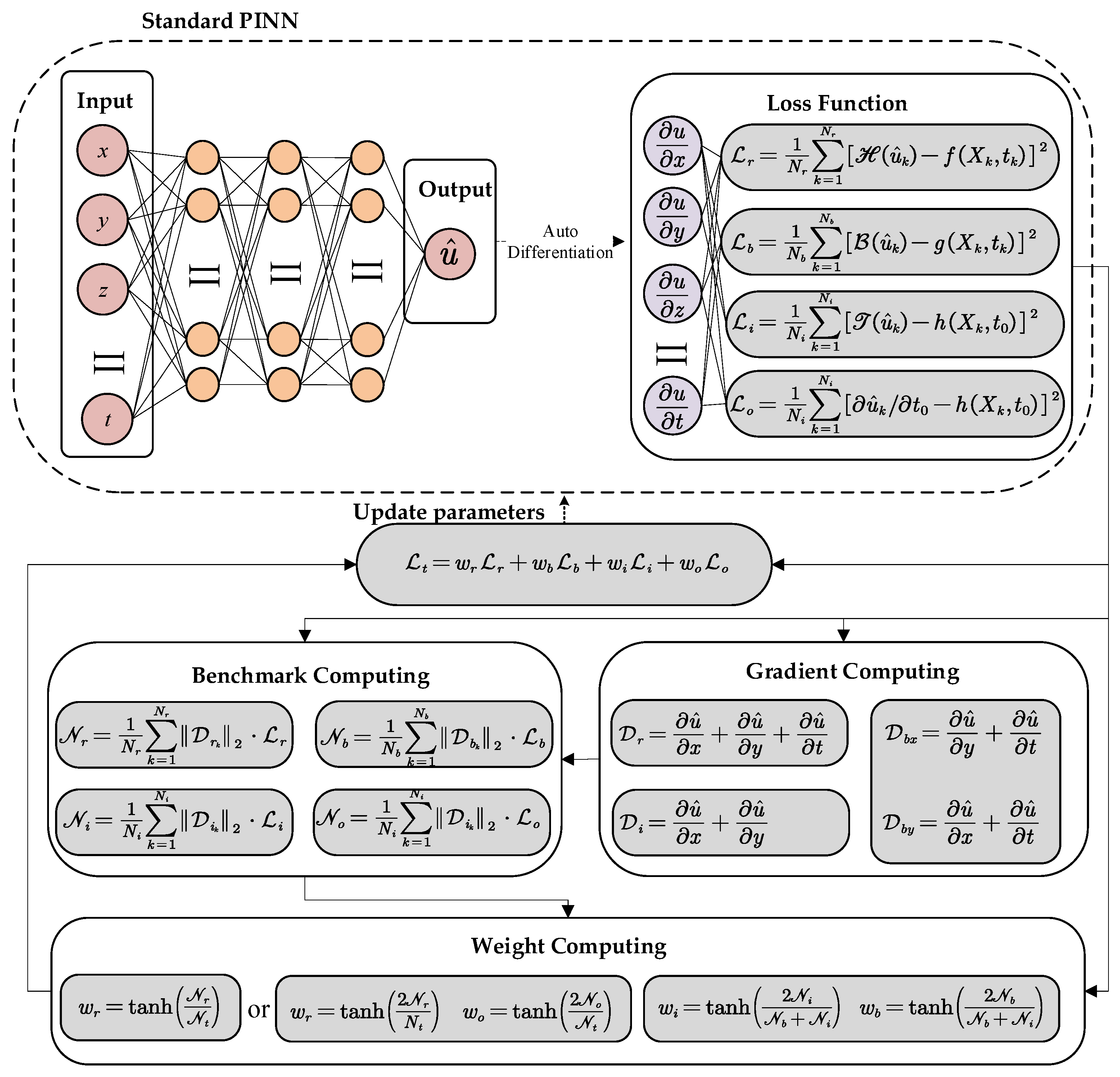
As illustrated in Figure 1, the DDR-PINN extends the standard PINN framework by computing the dot product between the gradient and unit vectors in different domains. The dot product of the gradient and the unit vector simultaneously reflect both the direction and magnitude of the projection of the solution function, but it is limited by convergence fluctuations. To avoid introducing extra training conflicts, we use the hyperbolic tangent function to map the L₂ norm to the $(0,1)$ within each domain, and finally obtain the weights for each loss term.

Figure 1. The framework of DDR-PINN.

The gradient of $\widehat{u}=\mathcal{N}\left(u\left(x,t\right);\lambda \right)$ is as follows:

$$\nabla \widehat{u}=\left({\displaystyle \frac{\partial \widehat{u}}{\partial X}},{\displaystyle \frac{\partial \widehat{u}}{\partial t}}\right).$$

(6)

For example, when considering a two-dimensional PDE, Equation (6) can be expressed as follows:

$$\nabla \widehat{u}=\left({\displaystyle \frac{\partial \widehat{u}}{\partial x}},{\displaystyle \frac{\partial \widehat{u}}{\partial y}},{\displaystyle \frac{\partial \widehat{u}}{\partial t}}\right).$$

(7)

Here, the gradient is represented as a vector. Since the dot product can be interpreted as the projection of one vector onto another multiplied by its magnitude, we compute the dot product between the solution $\nabla \widehat{u}$ and the unit vector, to quantify the variation intensity of the gradient along the direction of the unit vector. Furthermore, as the $\partial \widehat{u}/\partial x=0,\partial \widehat{u}/\partial y=0$ on the boundary domain, and $\partial \widehat{u}/\partial t=0$ on the initial domain, the dot product results in the interior domain, boundary domain, and initial domain are as follows:

$${\mathcal{D}}_r={\displaystyle \frac{\partial \widehat{u}}{\partial x}}+{\displaystyle \frac{\partial \widehat{u}}{\partial y}}+{\displaystyle \frac{\partial \widehat{u}}{\partial t}},$$

(8)

$${\mathcal{D}}_{bx}={\displaystyle \frac{\partial \widehat{u}}{\partial y}}+{\displaystyle \frac{\partial \widehat{u}}{\partial t}},$$

(9)

$${\mathcal{D}}_{by}={\displaystyle \frac{\partial \widehat{u}}{\partial x}}+{\displaystyle \frac{\partial \widehat{u}}{\partial t}},$$

(10)

$${\mathcal{D}}_i={\displaystyle \frac{\partial \widehat{u}}{\partial x}}+{\displaystyle \frac{\partial \widehat{u}}{\partial y}},$$

(11)

where ${\mathcal{D}}_r$, ${\mathcal{D}}_i$ are dot product results in the interior, initial domain, and ${\mathcal{D}}_{bx}$, ${\mathcal{D}}_{by}$ are dot products in the $x$ boundary and $y$ boundary, respectively. Then, ${\mathcal{D}}_b={\left[{\mathcal{D}}_{bx,}{\mathcal{D}}_{by}\right]}^{\mathrm{T}}$.

To ensure that residual information directly influences the weights without misleading effects, we directly multiply the square of the residual by the average of the L₂ norm of the dot product. The aim of the square term is to amplify high residuals and attenuate low residuals, guiding the PINN convergence.

$${\mathcal{N}}_r={\displaystyle \frac{1}{N_r}}{\displaystyle \sum _{k=1}^{N_r}\Vert {\mathcal{D}}_{r_k}{\Vert }_2}\cdot {\mathcal{L}}_r,$$

(12)

$${\mathcal{N}}_b={\displaystyle \frac{1}{N_b}}{\displaystyle \sum _{k=1}^{N_b}\Vert {\mathcal{D}}_{b_k}{\Vert }_2}\cdot {\mathcal{L}}_b,$$

(13)

$${\mathcal{N}}_i={\displaystyle \frac{1}{N_i}}{\displaystyle \sum _{k=1}^{N_i}\Vert {\mathcal{D}}_{i_k}{\Vert }_2}\cdot {\mathcal{L}}_i,$$

(14)

$${\mathcal{N}}_t={\mathcal{N}}_r+{\mathcal{N}}_b+{\mathcal{N}}_i,$$

(15)

where ${\mathcal{N}}_r$, ${\mathcal{N}}_b$, ${\mathcal{N}}_i$ are the gradient-residual benchmark in interior, boundary and initial domains, respectively.

Here is the Dirichlet boundary example. To unify the magnitude of the weights and distinguish the PDE residual from the solution residual, we adopt two different equations for computing the PDE and boundary weights. The number of sampling points, as well as the magnitude of residuals and fluctuations in the interior domain, are typically much larger than those on the boundary. And the interior residual corresponds to the PDE loss, rather than a solution-value loss. Therefore, we use the overall proportion of interior domain samples as the baseline value for weighting. In contrast, the boundary and the initial domain loss both represent solution residuals, thus we treat them as a unified group. Finally, we apply a tanh transformation as a nonlinear smoothing to improve the situation that the basic raw proportions lead to large fluctuations. Meanwhile, the variation in tanh is relatively small within the interval $[0,0.5]$, so we multiply the baseline value of the boundary and initial terms by a constant 2. The weights of loss terms under the Dirichlet boundary are as shown in Equations (16)–(18).

$$w_r=\tan \mathrm{h}\left({\displaystyle \frac{{\mathcal{N}}_r}{{\mathcal{N}}_t}}\right),$$

(16)

$$w_b=\tan \mathrm{h}\left({\displaystyle \frac{2{\mathcal{N}}_b}{{\mathcal{N}}_b+{\mathcal{N}}_i}}\right),$$

(17)

$$w_i=\tan \mathrm{h}\left({\displaystyle \frac{2{\mathcal{N}}_i}{{\mathcal{N}}_b+{\mathcal{N}}_i}}\right),$$

(18)

$${\mathcal{L}}_t=w_r{\mathcal{L}}_r+w_b{\mathcal{L}}_b+w_i{\mathcal{L}}_i,$$

(19)

where $w_r$, $w_r$, and $w_r$ are the weights of ${\mathcal{L}}_r$${\mathcal{L}}_r$${\mathcal{L}}_r$ respectively.

For the Neumann boundary condition, it involves the derivative of the solution function. For instance, the constraints of the wave equation include the initial velocity. And the residual of the initial velocity corresponds to the partial derivative of the solution with respect to the independent variable. Thus, the initial velocity loss can be aligned with the PDE loss. Furthermore, we multiply the baseline value of the PDE loss and the initial velocity loss by a constant of 2 so that they are the same as other loss weights. The weights of loss terms under the Neumann boundary condition are given as follows:

$${\mathcal{N}}_o={\displaystyle \frac{1}{N_i}}{\displaystyle \sum _{k=1}^{N_i}\Vert {\mathcal{D}}_{i_k}{\Vert }_2}\cdot {\mathcal{L}}_o$$

(20)

$${\mathcal{L}}_o={\displaystyle \frac{1}{N_i}}{\displaystyle \sum _{k=1}^{N_i}{\left[\partial {\widehat{u}}_k/\partial t_0-h\left(X_k,t_0\right)\right]}^2}$$

(21)

$${\mathcal{N}}_t={\mathcal{N}}_r+{\mathcal{N}}_b+{\mathcal{N}}_i+{\mathcal{N}}_o$$

(22)

$$w_r=\tan \mathrm{h}\left({\displaystyle \frac{2{\mathcal{N}}_r}{N_t}}\right),$$

(23)

$$w_o=\tan \mathrm{h}\left({\displaystyle \frac{2{\mathcal{N}}_o}{{\mathcal{N}}_t}}\right),$$

(24)

$${\mathcal{L}}_t=w_r{\mathcal{L}}_r+w_b{\mathcal{L}}_b+w_i{\mathcal{L}}_i+w_o{\mathcal{L}}_o,$$

(25)

where ${\mathcal{N}}_t={\mathcal{N}}_r+{\mathcal{N}}_b+{\mathcal{N}}_i+{\mathcal{N}}_o$, and ${\mathcal{N}}_o={\displaystyle \frac{1}{N_i}}{\displaystyle \sum _{k=1}^{N_i}\Vert {\mathcal{D}}_{i_k}{\Vert }_2}\cdot {\mathcal{L}}_o$. Taking the wave equation as an example, the initial velocity restricts the partial derivative of the solution function in the initial domain with respect to t and the loss fluctuation of the solution function is still reflected in the initial domain. Thus, we still adopt ${\mathcal{D}}_{i_k}$ for this part. Meanwhile, the additional loss term corresponds to the mean squared residual of the initial velocity ${\mathcal{L}}_o={\displaystyle \frac{1}{N_i}}{\displaystyle \sum _{k=1}^{N_i}{\left[\partial {\widehat{u}}_k/\partial t_0-h\left(X_k,t_0\right)\right]}^2}$.

4. Experiments

To evaluate the performance of the DDR-PINN, six PDEs covering 1D, 2D and 3D cases of two typical physical scenarios, heat equations and wave equations, are solved in experiments. In accordance with practical application requirements, all PDEs are inhomogeneous to characterize the existence of external or interior disturbance factors. The DDR-PINN is compared with three representative PINNs: the standard PINN [32] serves as the general benchmark, the APINN [26] as the benchmark for weight-optimized PINNs, and the VI-PINN [25] as the benchmark for loss function-optimized PINNs.

4.1. Setup

All PINNs adopted the same network architecture with 3 hidden layers with 30 neurons per layer, and the activation function is tanh. The optimizer is Adam. In addition, since PINNs sample different spatiotemporal points for the discretization of training and evaluation in the process of solving PDEs, the randomness of sampling and training may lead to unfair discrepancies among different experimental PINNs. To eliminate this potential unfairness, network parameters were initialized with the same random seed. To raise training efficiency, we adopt a step decay learning rate strategy where the initial learning rate is set to 0.001, and it is halved every 2000 training epochs. For each case, we present the exact solution and compare the solutions computed by the PINNs. All input coordinate points are randomly sampled within the domains, with the specific sampling sizes of the training set detailed in Table 1. The sampling ratio across distinct domains is kept consistent with that of the training set. There are 1000 points extracted from the test set to monitor model performance, which are exclusively used for mean squared error (MSE) evaluation. All PINNs were trained on an NVIDIA RTX 3060 graphics card. The Compute Unified Device Architecture (CUDA) library of the Graphics Processing Unit (GPU) was utilized to accelerate the computational speed, and the machine learning framework PyTorch 2.5.1 was adopted to construct the PINN frameworks.

Table 1. Hyperparameter settings for different PDEs. Here, N_r, N_b, N_i, N_t are the number of sampling points in the interior domain, boundary, initial, and test domain. $\lambda$ is the hyperparameter of the modified negative log-likelihood in VI-PINN. N_a is the hyperparameter of updating learning speed in APINN. The $\lambda$ and N_a are consistent with the original reference setting. Here 1D-H denotes the heat equation under 1D condition, and 1D-W denotes the wave equation under 1D condition. Similarly, the others with prefix 2D and 3D are heat equations and wave equations under 2D and 3D conditions.

PDEs	Epochs	Sampling Points				$\mathbf{VI-PINNs}(\mathit{\lambda }$)	APINN (Na)
		Nr	Nb	Ni	Nt
1D-H	1 × 104	2 × 103	2 × 102	2 × 102	5 × 103	2 × 10−3	50
1D-W	1.5 × 104	2 × 103	2 × 102	2 × 102	5 × 103	5 × 10−5	50
2D-H	2 × 104	2 × 103	4 × 102	2 × 102	5 × 103	2 × 10−3	50
2D-W	2 × 104	2 × 103	4 × 102	2 × 102	5 × 103	5 × 10−5	50
3D-H	2.5 × 104	3 × 103	6 × 102	3 × 102	1 × 104	2 × 10−3	50
3D-W	2.5 × 104	3 × 103	6 × 102	3 × 102	1 × 104	5 × 10−5	50

4.2. Evaluation Metrics

We adopted two metrics, the MSE and L₂-error (L₂), and trainable parameters to evaluate the performance of all PINNs.

$$MSE={\displaystyle \frac{1}{N}}{\displaystyle \sum _{i=1}^N{\left(u_i-\widehat{u}\right)}^2},$$

(26)

$$L_2-Error={\displaystyle \frac{\left|\right|u-\widehat{u}|{|}_2}{\left|\right|u|{|}_2}},$$

(27)

where $\left|\right|\cdot \left|\right|$ is the L2 norm. The evaluation results were as shown in Table 2.

Table 2. MSE and L2-error of different PDEs. Here, par is short for trainable parameters. Here 1D-H denotes the heat equation under 1D condition, and 1D-W denotes the wave equation under 1D condition. Similarly, the others with prefix 2D and 3D are heat equations and wave equations under 2D and 3D conditions.

PDEs	Standard PINN			VI-PINN			APINN			DDR-PINN
	MSE	L2	Par	MSE	L2	Par	MSE	L2	Par	MSE	L2	Par
1D-H	1.22 × 10−4	2.71 × 10−2	2911	1.00 × 10−5	7.94 × 10−3	2022	3.10 × 10−5	1.38 × 10−2	1981	6.00 × 10−6	6.2 × 10−3	1981
1D-W	1.48 × 10−4	5.29 × 10−2	2911	1.15 × 10−4	4.67 × 10−2	2012	1.32 × 10−3	1.58 × 10−1	1981	3.80 × 10−5	2.69 × 10−2	1981
2D-H	1.79 × 10−4	7.14 × 10−3	2941	7.10 × 10−5	4.49 × 10−3	2042	7.25 × 10−4	1.44 × 10−2	2011	5.00 × 10−5	3.76 × 10−3	2011
2D-W	2.29 × 10−4	5.79 × 10−1	2941	1.71 × 10−4	5.01 × 10−1	2042	2.31 × 10−4	5.82 × 10−1	2011	1.55 × 10−4	4.77 × 10−1	2011
3D-H	9.34 × 10−3	1.23 × 10−1	2971	2.86 × 10−3	6.82 × 10−2	2072	3.47 × 10−3	7.51 × 10−2	2041	1.37 × 10−3	4.71 × 10−2	2041
3D-W	9.10 × 10−5	5.18 × 10−1	2971	7.70 × 10−5	4.76 × 10−1	2072	9.80 × 10−5	5.37 × 10−1	2041	7.60 × 10−5	4.71 × 10−1	2041

4.3. 1D Heat Equation

The heat equation is a typical case of parabolic PDEs, and its solution can describe the time-dependent temperature distribution. The case with a source term is as follows:

$$u_t+u_x=0.005u_{xx}+2\pi \left(1-x\right)\cos \left(2\pi t\right)-\sin \left(2\pi t\right),xϵ\left[0,1\right],tϵ\left[0,2\right],$$

(28)

$$\left\{\begin{array}{l}u\left(0,t\right)=\sin \left(2\pi t\right)\hfill \\ u\left(1,t\right)=0\hfill \\ u\left(x,0\right)=0\hfill \end{array}\right.,$$

(29)

$$u\left(x,y\right)=\left(1-x\right)\sin \left(2\pi t\right),xϵ\left[0,1\right],tϵ\left[0,2\right].$$

(30)

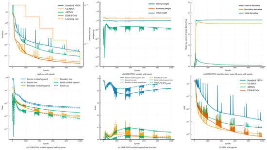
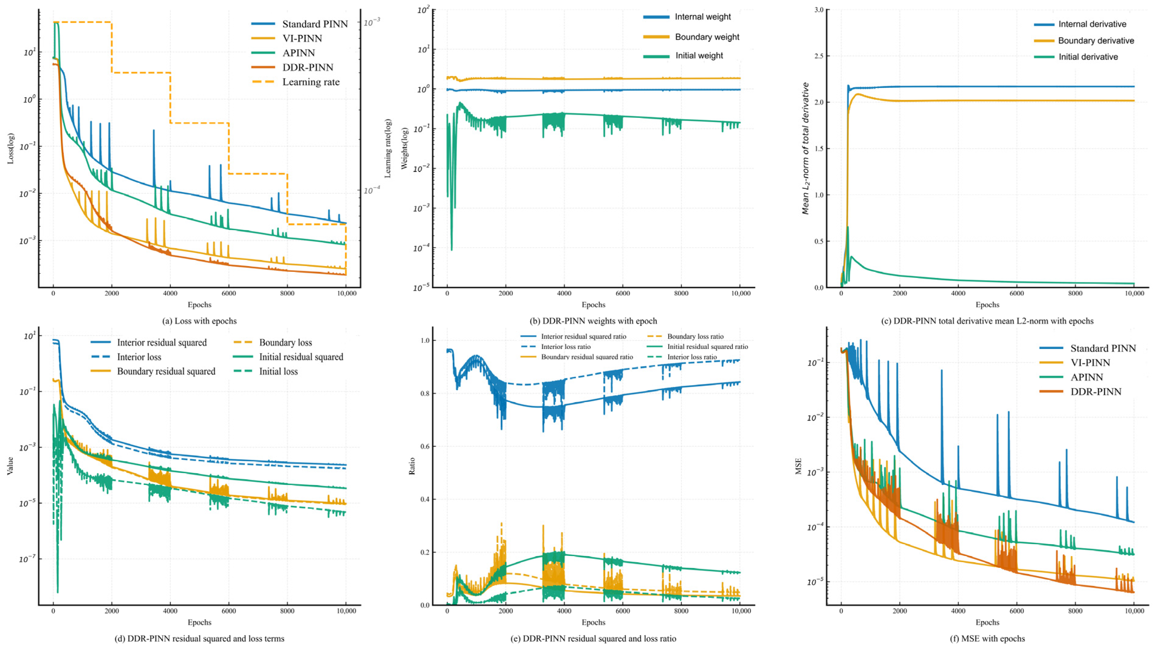
In Figure 2a, the DDR-PINN achieves faster convergence, showing the smallest fluctuation. It can be clearly observed from Figure 2d that the primary parts causing fluctuations in the DDR-PINN are the boundary and initial domain. The value of the loss term becomes much smoother after the product operation between squared residuals and adaptive weights in Figure 2b. In Figure 2c, it can be seen that the variation in the mean L₂ norm of the total derivative is relatively stable, except that the initial derivative domain undergoes a brief period with intense fluctuation in the early stage. Figure 2e shows that the proportional changes between residuals squared and loss, revealing that the interior domain dominates, followed by the boundary domain and the initial domain.

Figure 2. The process of PINNs for solving 1D heat equation: (a) all PINN loss, (b) DDR-PINN weights and learning rate with epochs, (c) DDR-PINN total derivative mean L2-norm, (d) DDR-PINN loss terms and residual values, (e) DDR-PINN loss ratio and residual ratio, (f) all PINNs MSE in the test set.

As illustrated in Figure 3, the exact solution exhibits distinct spatiotemporal evolution characteristics. Since dimensionless data are typically used in solving PDEs, negative values in the solution indicate temperatures below the reference value. In terms of extreme error values, the APINN performs the best, with a maximum absolute error of 0.018, and both the VI-PINN and DDR-PINN have 0.02. The errors of the DDR-PINN are uniformly distributed, and extreme errors occur with lower frequencies across the entire spatiotemporal domain, without exhibiting an obvious tendency for errors to increase with time.

Figure 3. The PINN solutions of the 1D heat equation: (a) standard PINN solution, (b) VI-PINN solution, (c) APINN absolute error, (d) DDR-PINN solution, (e) standard PINN absolute error, (f) VI-PINN absolute error, (g) APINN absolute error, (h) DDR-PINN absolute error.

4.4. 1D Wave Equation

The wave equation is a typical case of hyperbolic equations, which is used to describe the spatiotemporal distribution of various wave phenomena. To reflect the periodic variation in the equation, we selected one and a half periods in the time dimension. To adapt to the second-order characteristics of the wave equation and ensure the fairness of comparative experiments, we increased the number of epochs to 15,000, so that all PINNs can fully converge.

$${\displaystyle \frac{{\partial }^{2}u}{\partial t^2}}={\displaystyle \frac{{\partial }^{2}u}{\partial x^2}}+{\pi }^{2}x\left(1-x\right)\cos \left(\pi t\right)-2\cos \left(\pi t\right)+2,tϵ\left[0,3\right],xϵ\left[0,1\right].$$

(31)

$$u\left(0,t\right)=u\left(1,t\right)=u\left(x,0\right)=u{\left(0,x\right)}_t=0,$$

(32)

where the $u{\left(0,x\right)}_t$ denotes the initial velocity, which is a necessary condition for the wave equation to have a unique solution.

$$u\left(t,x\right)=x\left(1-x\right)\left[1-\cos \left(\pi t\right)\right],tϵ\left[0,3\right],xϵ\left[0,1\right].$$

(33)

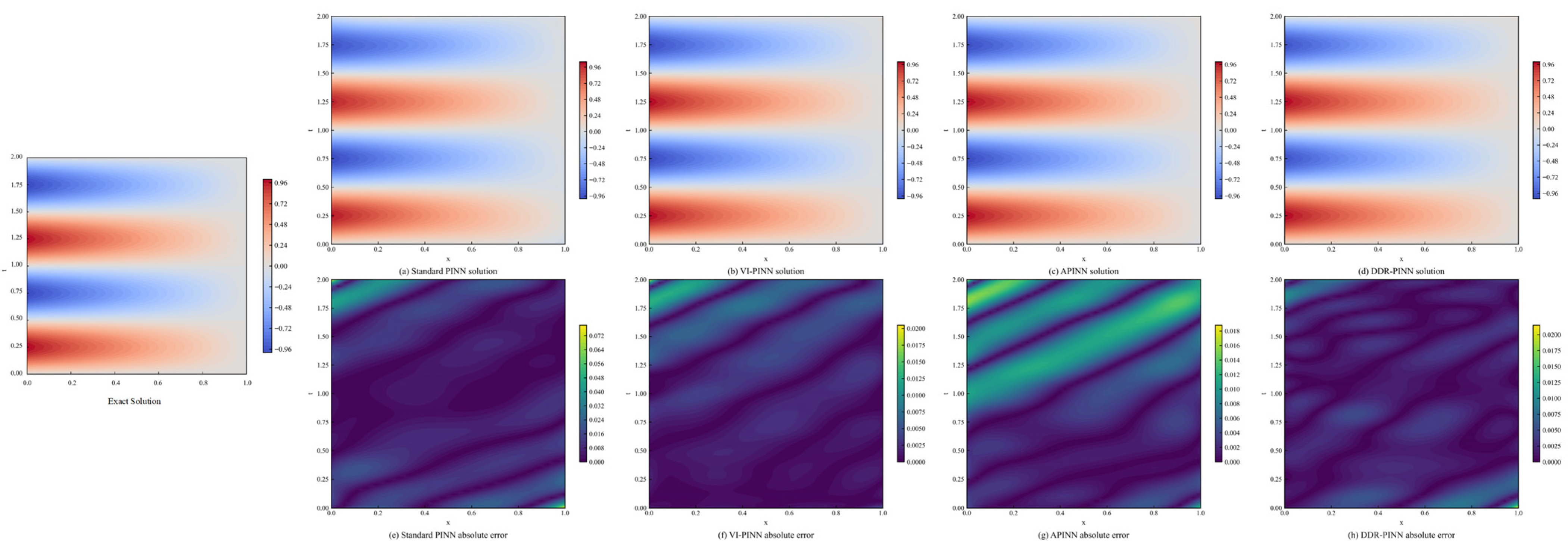
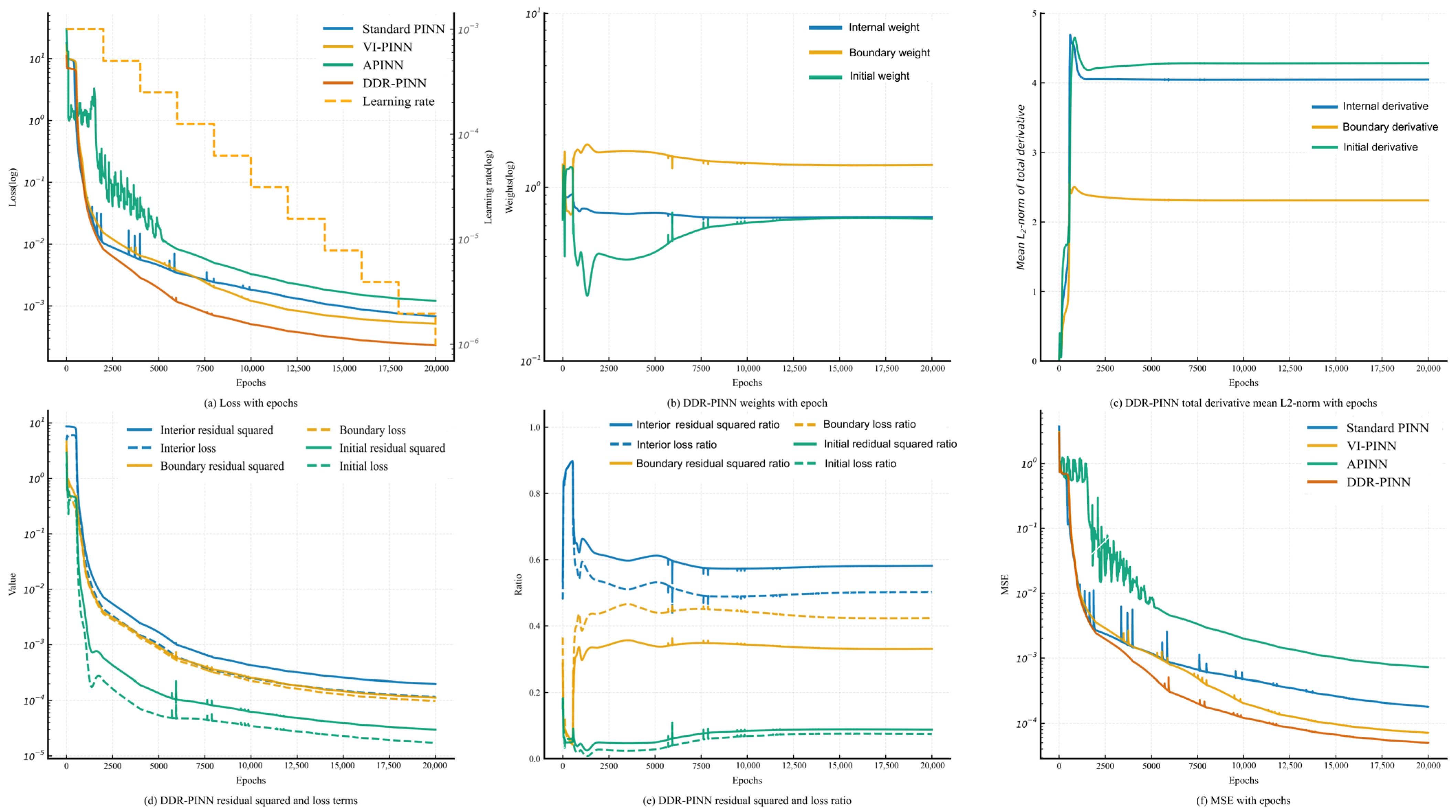
As observed in Figure 4a, DDR-PINNs exhibit a relatively fast convergence process with minor fluctuations. It should be noted that, according to the analysis of Figure 4b, after 4000 epochs, the weights of the initial domain, boundary domain, and interior domain tend to stabilize. Therefore, the residuals of the boundary and initial domains, as well as the PDE residuals of the interior domain, are the main components contributing to the loss. As can be clearly observed in Figure 4d, the reweighting of the DDR-PINN exerts a significant impact on the initial domain. In contrast, the interior domain and boundary domain are barely affected. Finally, as can be observed in Figure 4f, after 3000 training iterations, the DDR-PINN performs the best among all PINNs and maintains its leading position consistently.

Figure 4. The process of PINNs for solving 1D wave equation: (a) all PINN loss, (b) DDR-PINN weights and learning rate with epochs, (c) DDR-PINN total derivative mean L2-norm, (d) DDR-PINN loss terms and residual values, (e) DDR-PINN loss ratio and residual ratio, (f) all PINNs MSE in the test set.

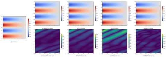
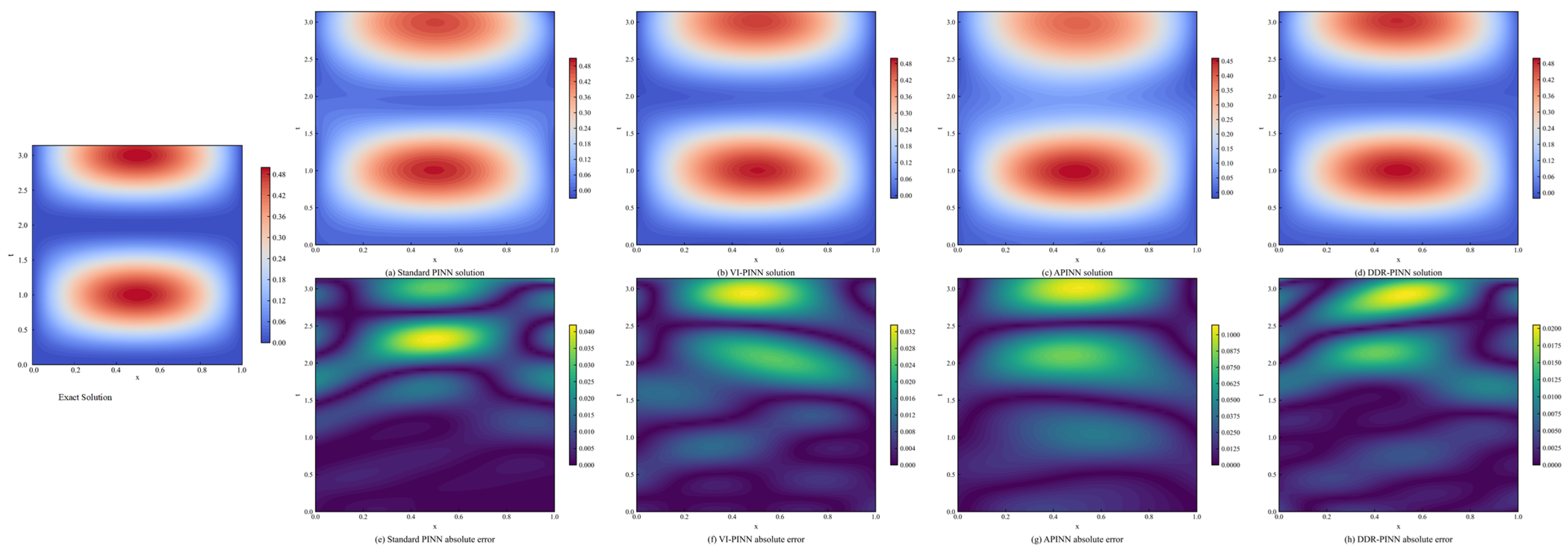
As shown in Figure 5, the exact solution of the 1D wave equation exhibits distinct peaks and valleys. According to the exact solution, the period of the 1D wave equation is 2, so the solution shows obvious periodicity over time within the time interval [0, 2] at the same spatial point. Meanwhile, the solution also presents fluctuation phenomena with spatial variation and is symmetric about x = 0.5 at the same time point. Figure 5 also presents the 1D wave equation solution absolute errors of different PINNs. The maximum value of the absolute error is 0.1, occurring in the APINN, while the maximum value of the absolute error in the DDR-PINN is 0.02. Overall, the absolute errors of all PINNs exhibit a tendency to expand with the increase in time, reaching the maximum at the upper time boundary. And the solution also attains local minima at the moments of period transition (t = 2).

Figure 5. The PINN solutions of the 1D wave equation: (a) standard PINN solution, (b) VI-PINN solution, (c) APINN absolute error, (d) DDR-PINN solution, (e) standard PINN absolute error, (f) VI-PINN absolute error, (g) APINN absolute error, (h) DDR-PINN absolute error.

4.5. 2D Heat Equation

The 2D heat transfer conduction–diffusion equation exhibits convection effects in two directions. Additionally, we set a time-varying heat source and boundary conditions:

$${\displaystyle \frac{\partial u}{\partial t}}+0.2{\displaystyle \frac{\partial u}{\partial x}}+0.1{\displaystyle \frac{\partial u}{\partial y}}=0.1({\displaystyle \frac{{\partial }^{2}u}{\partial x^2}}+{\displaystyle \frac{{\partial }^{2}u}{\partial y^2}})+S,tϵ\left[0,2\right],x,yϵ\left[0,1\right],$$

(34)

where the $S=y^2\cos \left(t\right)-0.4\pi \sin \left(2\pi x\right)+0.4{\pi }^2\cos \left(2\pi x\right)+0.2\left(1-y\right)\left[1-\sin \left(t\right)\right]$.

$$\left\{\begin{array}{l}u\left(0,y,t\right)=u\left(1,y,t\right)=y^2\sin \left(t\right)-y^2+3\hfill \\ u\left(x,0,t\right)=\cos \left(2\pi x\right)+2\hfill \\ u\left(x,1,t\right)=\cos \left(2\pi x\right)+\sin \left(t\right)+1\hfill \\ u\left(x,y,0\right)=\cos \left(2\pi x\right)-y+2\hfill \end{array}\right.,$$

(35)

$$u\left(x,y,t\right)=\cos \left(2\pi x\right)+y^2\sin \left(t\right)-y^2+2,tϵ\left[0,2\pi \right],x,yϵ\left[0,1\right].$$

(36)

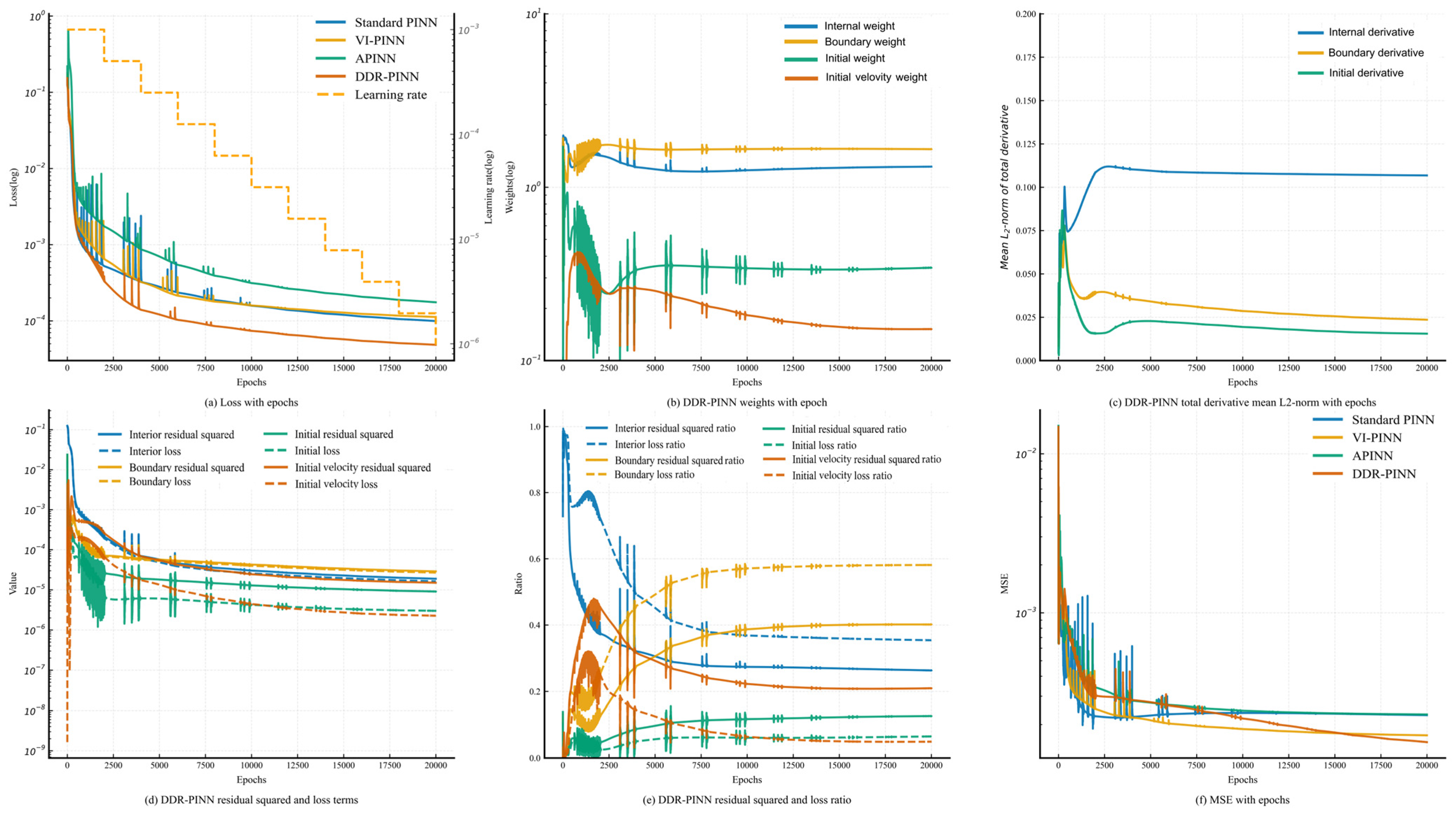
To solve the 2D PDE, we increased the number of training iterations to 20,000 again to ensure all of the PINNs fully converge. As shown in Figure 6a, the DDR-PINN still exhibits the best convergence stability and speed during the loss reduction process. In Figure 6c, the overall solution process is dominated by the interior domain, with the boundary domain ranking second by a narrow margin to the interior domain and the initial domain exerts a minor influence. Figure 6d illustrates that the influence of the interior domain and initial domain is reduced while the boundary domain is maintained after reweighting, resulting in the interior domain and boundary domain being basically at the same loss magnitude. This indicates that the PDE solution is significantly affected by the boundary, which is consistent with the complex boundary condition given above. As reflected in Figure 6f, the solution accuracy of both the APINN and the standard PINN fluctuates generally, while the VI-PINN and DDR-PINN show smaller fluctuations, and the DDR-PINN achieves the highest solution accuracy.

Figure 6. The process of PINNs for solving 2D heat equation: (a) all PINN loss, (b) DDR-PINN weights and learning rate with epochs, (c) DDR-PINN total derivative mean L2-norm, (d) DDR-PINN loss terms and residual values, (e) DDR-PINN loss ratio and residual ratio, (f) all PINNs MSE in the test set.

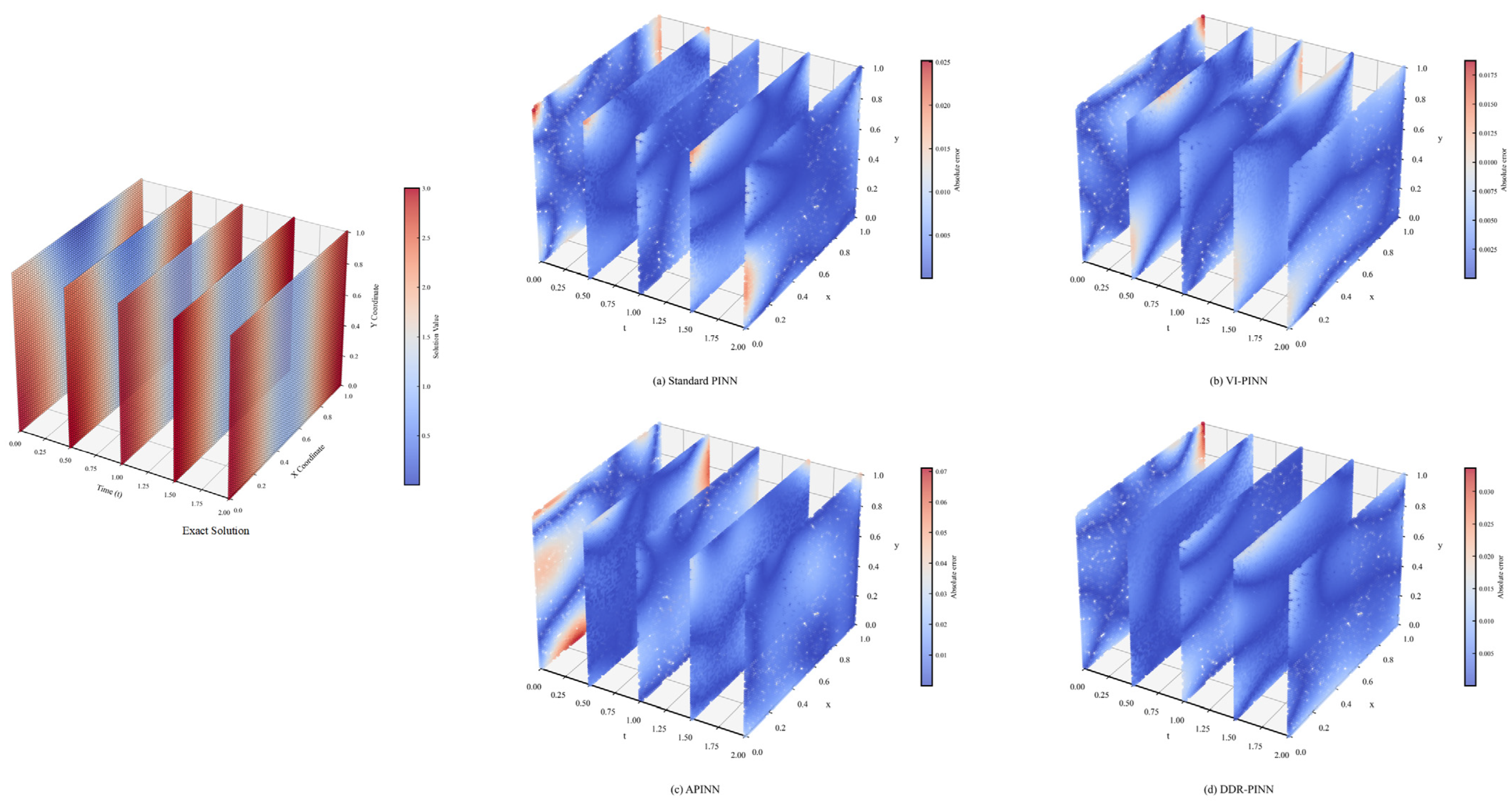
As illustrated in Figure 7, the exact solution of the 2D heat equation is visualized at 5 time slices, which are $t=\left[0,0.5,1,1.5,2\right]$. It can be seen that at each time slice, both the upper and lower boundaries of the solution exhibit periodic variations, while the left and right boundaries undergo constant heating. Additionally, with the passage of time, heat diffuses from the boundaries toward the center. It should be noted that the evaluation metric is calculated over the full-time domain, and only 5 time points are displayed here for clarity. The maximum absolute error is 0.07, occurring in the APINN, while the VI-PINN achieves the smallest maximum absolute error of 0.0175. For the standard PINN and DDR-PINN, their maximum absolute errors are 0.025 and 0.030, respectively. In terms of error distribution, the absolute errors of all PINNs are mainly concentrated in the boundary domain. For the DDR-PINN, the absolute errors are mainly concentrated on the right boundary at the initial time, with few errors distributed at other time points, demonstrating overall excellent solution accuracy.

Figure 7. The absolute error of PINN solutions for the 2D heat equation: (a) standard PINN solution absolute error, (b) VI-PINN solution absolute error, (c) APINN solution absolute error, (d) DDR-PINN solution absolute error.

4.6. 2D Wave Equation

To simulate practical application requirements, the 2D wave equation has a source term, and both initial conditions and initial velocity are 0, which is consistent with the conventional conditions of the wave equation:

$${\displaystyle \frac{{\partial }^{2}u}{\partial t^2}}={\displaystyle \frac{{\partial }^{2}u}{\partial x^2}}+{\displaystyle \frac{{\partial }^{2}u}{\partial y^2}}+\sin \left(\pi x\right)\sin \left(\pi y\right)\sin \left({\displaystyle \frac{\sqrt{2}}{2}}\pi t\right),tϵ\left[0,2\sqrt{2}\right],x,yϵ\left[0,1\right].$$

(37)

$$\left\{\begin{array}{l}u\left(0,y,t\right)=u\left(1,y,t\right)=u\left(x,0,t\right)=u\left(x,1,t\right)=u\left(x,y,0\right)=0\hfill \\ u{\left(x,y,0\right)}_t=0\hfill \end{array}\right.,$$

(38)

where the $u{\left(x,y,0\right)}_t$ denotes the initial velocity.

$$u\left(x,y,t\right)={\displaystyle \frac{2}{3{\pi }^2}}\sin \left(\pi x\right)\sin \left(\pi y\right)\left[\sin \left({\displaystyle \frac{\sqrt{2}}{2}}\pi t\right)-{\displaystyle \frac{1}{2}}\sin \left(\sqrt{2}\pi t\right)\right],tϵ\left[0,2\sqrt{2}\right],xϵ\left[0,1\right],yϵ\left[0,1\right].$$

(39)

As shown in Figure 8a, compared with the 2D heat equation, the losses of all PINNs when solving the 2D wave equation exhibit more intense fluctuations during the training process. The DDR-PINN exhibits the fastest and most stable loss reduction. According to Figure 8e, with the increase in epochs, the loss proportion of the interior domain and initial velocity decreases, while the loss proportion of the boundary and initial domain increases, resulting in a final situation that the boundary domain loss dominates, then the interior domain loss follows, and the loss of the initial domain and initial velocity are rank last with a similarly small magnitude. Based on analysis of Figure 8d, the reweighting of the DDR-PINN exerts the most significant influence on the initial conditions, including the initial domain and initial velocity, which reduces their values of the loss term. The reason is that both their derivative weights and residual values are relatively low.

Figure 8. The process of PINNs for solving the 2D wave equation: (a) all PINN loss, (b) DDR-PINN weights and learning rate with epochs, (c) DDR-PINN total derivative mean L2-norm, (d) DDR-PINN loss terms and residual values, (e) DDR-PINN loss ratio and residual ratio, (f) all PINNs MSE in the test set.

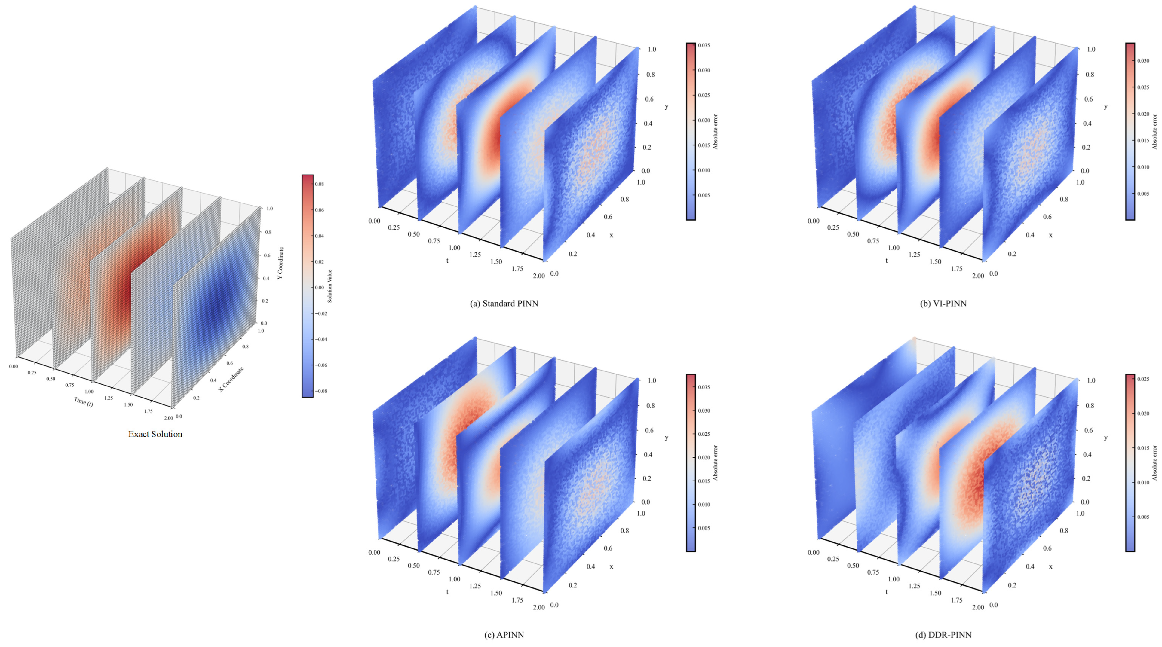
Figure 9 presents the exact solution of the 2D wave equation. For clarity of observation, we also selected 5 time slices $t=\left[0,0.5,1,1.5,2\right]$ to visualize. Since both the boundary and initial conditions are zero, the exact solution contains numerous zero-value domains. Meanwhile, it can be observed that the solution fluctuates between positive and negative values, exhibiting distinct oscillatory characteristics. Since the boundary conditions are zero, the errors are primarily focused on the central position of the interior domain. The DDR-PINN achieves the smallest maximum absolute error, 0.025. In terms of the temporal distribution, the absolute errors of the standard PINN, VI-PINN, and ACPINN are mainly concentrated at $t=\left\{0.5,1\right\}$, while the DDR-PINN’s errors are concentrated at $t=\left\{1,1.5\right\}$. Additionally, the DDR-PINN’s error is significantly smaller than that of the other PINNs at $t=2$.

Figure 9. The absolute error of PINN solutions for 2D wave equation: (a) standard PINN solution absolute error, (b) VI-PINN solution absolute error, (c) APINN solution absolute error, (d) DDR-PINN solution absolute error.

4.7. 3D Heat Equation

The heat source of the 3D heat equation is time-varying and periodically distributed in space.

$${\displaystyle \frac{\partial u}{\partial t}}+0.2{\displaystyle \frac{\partial u}{\partial x}}+0.1{\displaystyle \frac{\partial u}{\partial y}}+0.05{\displaystyle \frac{\partial u}{\partial z}}=0.1({\displaystyle \frac{{\partial }^{2}u}{\partial x^2}}+{\displaystyle \frac{{\partial }^{2}u}{\partial y^2}}+{\displaystyle \frac{{\partial }^{2}u}{\partial z^2}})+S,tϵ\left[0,2\pi \right],x,y,zϵ\left[0,1\right],$$

(40)

$$\left\{\begin{array}{l}{S}_1=\cos \left(t\right)-0.4\pi \sin \left(2\pi x\right)\cos \left(2\pi y\right)\cos \left(2\pi z\right)\hfill \\ S_2=-0.2\pi \cos \left(2\pi x\right)\sin \left(2\pi y\right)\cos \left(2\pi z\right)\hfill \\ S_3=-0.1\pi \cos \left(2\pi x\right)\cos \left(2\pi y\right)\sin \left(2\pi z\right)\hfill \\ S_4=1.2{\pi }^2\cos \left(2\pi x\right)\cos \left(2\pi y\right)\cos \left(2\pi z\right)\hfill \end{array}\right.,$$

(41)

where the $S=S_1+S_2+S_3+S_4$. The case boundary condition and exact solution are as follows:

$$\left\{\begin{array}{l}u\left(0,y,z,t\right)=u\left(1,y,z,t\right)=\cos \left(2\pi y\right)\cos \left(2\pi z\right)+\sin \left(t\right)\\ u\left(x,0,z,t\right)=u\left(x,1,z,t\right)=\cos \left(2\pi x\right)\cos \left(2\pi z\right)+\sin \left(t\right)\\ u\left(x,y,0,t\right)=u\left(x,y,1,t\right)=\cos \left(2\pi x\right)\cos \left(2\pi y\right)+\sin \left(t\right)\\ u\left(x,y,0\right)=\cos \left(2\pi x\right)\cos \left(2\pi y\right)\cos \left(2\pi z\right)\end{array}\right.$$

(42)

$$u\left(x,y,z,t\right)=\cos \left(2\pi x\right)\cos \left(2\pi y\right)\cos \left(2\pi z\right)+\sin \left(t\right),tϵ\left[0,2\pi \right],x,y,zϵ\left[0,1\right].$$

(43)

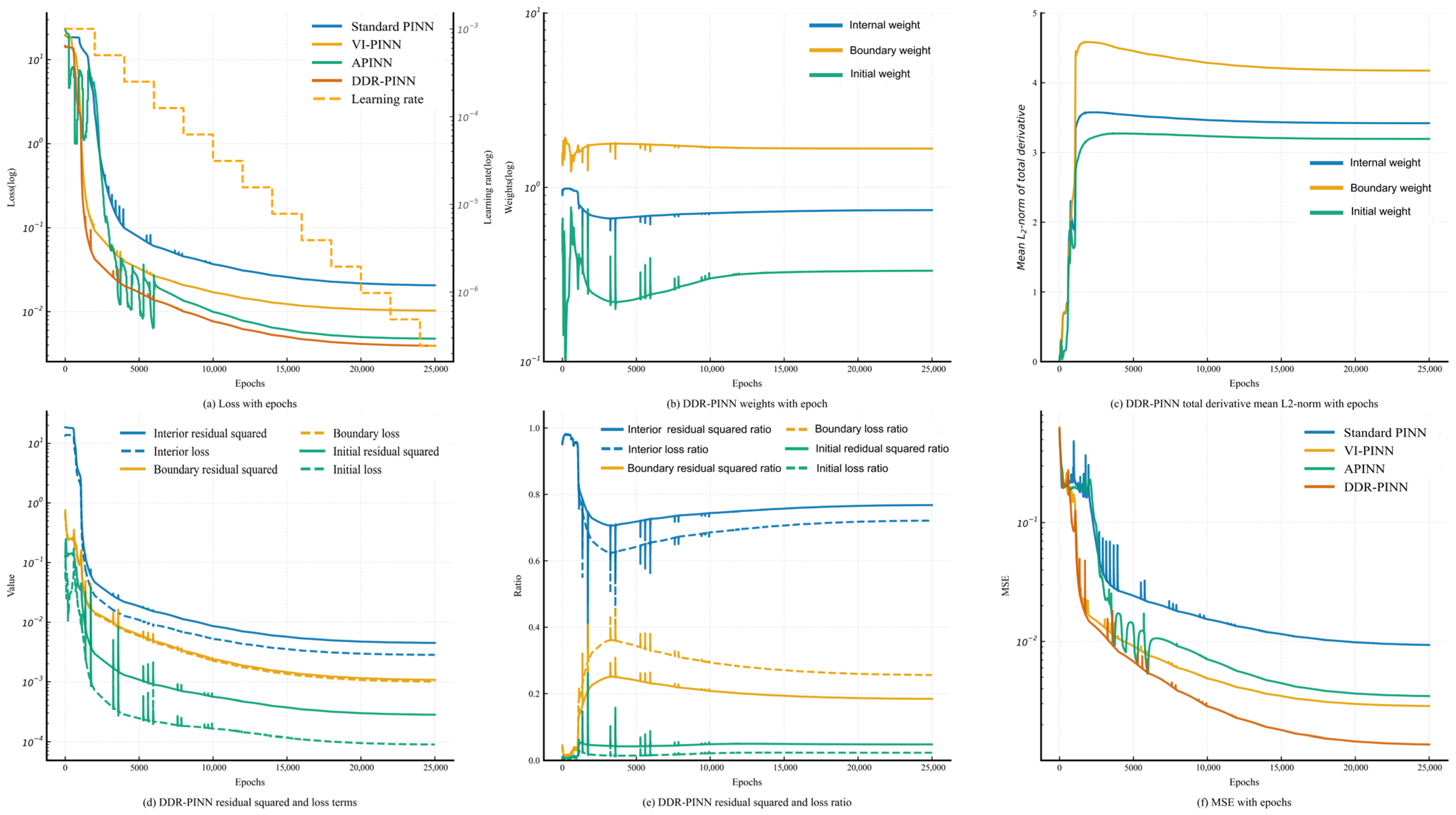
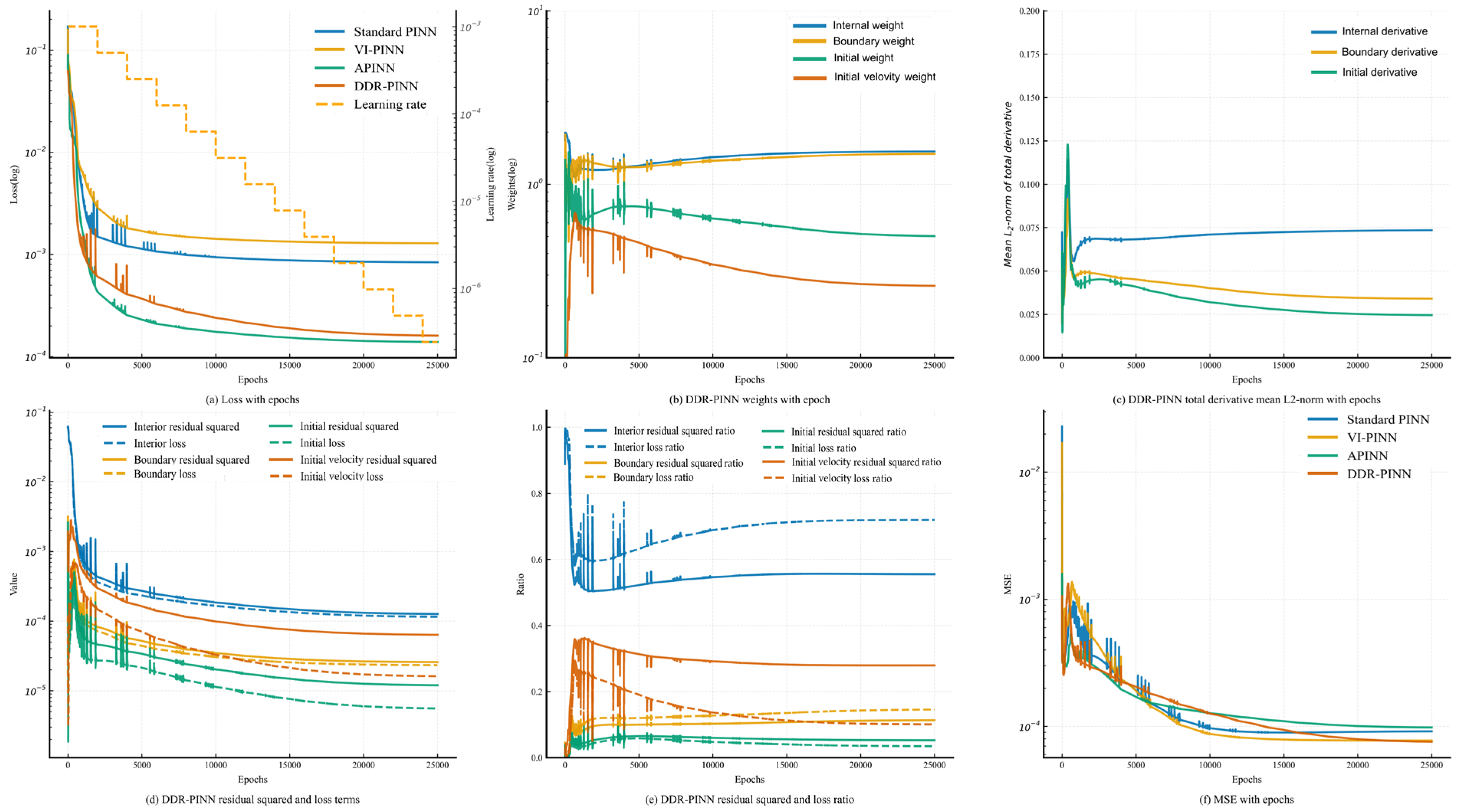
Figure 10 illustrates the solution process of the 3D heat equation. The number of epochs is increased to 25,000 for the stable convergence of PINNs. As shown in Figure 10a, the DDR-PINN exhibits the fastest convergence rate and superior stability, while the APINN delivers insufficient performance during training and in testing. We attribute this to the fact that multi-task learning fails to effectively balance the loss terms when dealing with multiple varying boundaries. This also demonstrates that if conflicts among loss terms are not alleviated adequately, the solution accuracy and efficiency will be significantly dropped, even resulting in a performance inferior to the standard PINN.

Figure 10. The process of PINNs for solving 3D heat equation: (a) all PINN loss, (b) DDR-PINN weights and learning rate with epochs, (c) DDR-PINN total derivative mean L2-norm, (d) DDR-PINN loss terms and residual values, (e) DDR-PINN loss ratio and residual ratio, (f) all PINNs MSE in the test set.

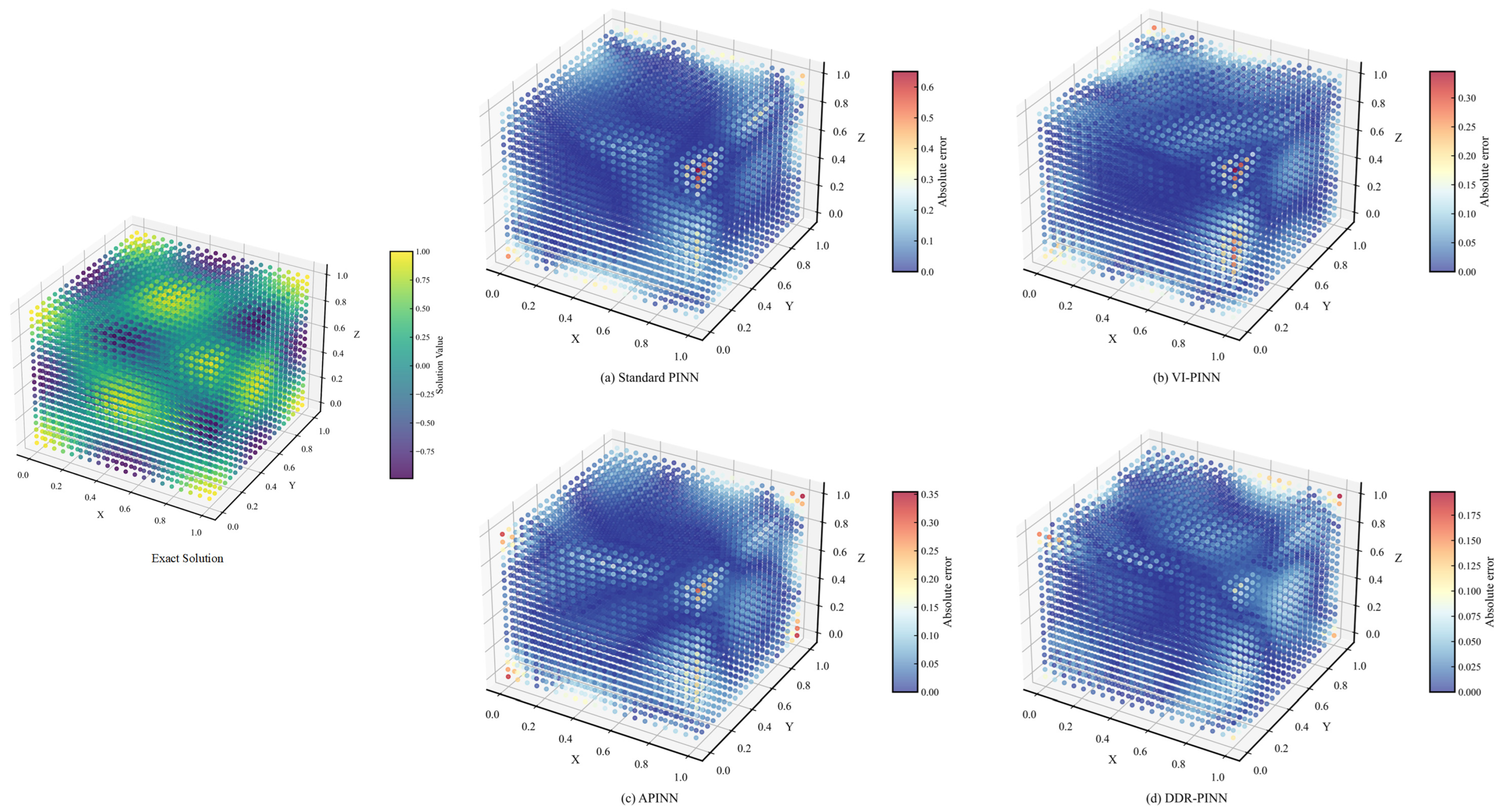
Figure 11 shows the exact solution and the results of PINNs for the 3D heat equation. Due to visualization constraints, we have only drawn the results at the intermediate time step (t = π). The solution of the PDE at the intermediate time step exhibits significant fluctuations with a maximum value of 1 and a minimum value of 0.75. The absolute errors of the DDR-PINN are relatively low, ranging from [0, 0.075]. The maximum absolute error is 0.6, located in the standard PINN, while the DDR-PINN achieves the smallest maximum absolute error of 0.175. Large errors of all PINNs are distributed at the boundaries, especially at the boundary intersections.

Figure 11. The absolute error of PINN solutions for 3D heat equation (t = π): (a) standard PINN solution absolute error, (b) VI-PINN solution absolute error, (c) APINN solution absolute error, (d) DDR-PINN solution absolute error.

4.8. 3D Wave Equation

The 3D wave equation is modified from the 2D wave equation. The boundary conditions include the Neumann boundary condition, the initial velocity, and Dirichlet conditions. The source term exhibits sinusoidal fluctuations spatiotemporally:

$${\displaystyle \frac{{\partial }^{2}u}{\partial t^2}}={\displaystyle \frac{{\partial }^{2}u}{\partial x^2}}+{\displaystyle \frac{{\partial }^{2}u}{\partial y^2}}+{\displaystyle \frac{{\partial }^{2}u}{\partial z^2}}+S,tϵ\left[0,\sqrt{2}\right],x,y,zϵ\left[0,1\right]$$

(44)

where $S=-\sin \left(\pi x\right)\sin \left(\pi y\right)\sin \left(\pi z\right)\sin \left(\sqrt{2}\pi t\right)$.

$$\left\{\begin{array}{l}u\left(0,y,z,t\right)=u\left(1,y,z,t\right)=0\hfill \\ u\left(x,0,z,t\right)=u\left(x,1,z,t\right)=0\hfill \\ u\left(x,y,0,t\right)=u\left(x,y,1,t\right)=0\hfill \\ u\left(x,y,z,0\right)=0\hfill \\ u{\left(x,y,z,0\right)}_t={\displaystyle \frac{\sqrt{3}-\sqrt{2}}{\pi }}\sin \left(\pi x\right)\sin \left(\pi y\right)\sin \left(\pi z\right)\hfill \end{array}\right.$$

(45)

$$u(x,y,z,t)={\displaystyle \frac{1}{{\pi }^2}}\mathrm{s}\mathrm{i}\mathrm{n}\left(\pi x\right)\mathrm{s}\mathrm{i}\mathrm{n}\left(\pi y\right)\mathrm{s}\mathrm{i}\mathrm{n}\left(\pi z\right)\left[\mathrm{s}\mathrm{i}\mathrm{n}\right(\sqrt{3}\pi t\left)-\mathrm{s}\mathrm{i}\mathrm{n}\right(\sqrt{2}\pi t\left)\right],tϵ[0,\sqrt{2}],x,y,zϵ[0,1]$$

(46)

As shown in Figure 12a, the APINN exhibits the fastest and most stable loss reduction, followed by the DDR-PINN, and then the standard PINN and VI-PINN in the process of solving the 3D wave equation. However, the APINN fails to achieve satisfactory solution accuracy on the test set. Similarly to the 3D heat equation, the multi-task mechanism of the APINN results in a degraded generalization ability. Relatively, the DDR-PINN has a slower convergence rate in the early stage. According to Figure 12b, we think the reason is that the large weight fluctuations of the DDR-PINN in the early stage lead to slow model learning efficiency. As the number of epochs increase, both the convergence rate and accuracy of the DDR-PINN are improved.

Figure 12. The process of PINNs for solving 3D wave equation: (a) all PINN loss, (b) DDR-PINN weights and learning rate with epochs, (c) DDR-PINN total derivative mean L2-norm, (d) DDR-PINN loss terms and residual values, (e) DDR-PINN loss ratio and residual ratio, (f) all PINNs MSE in the test set.

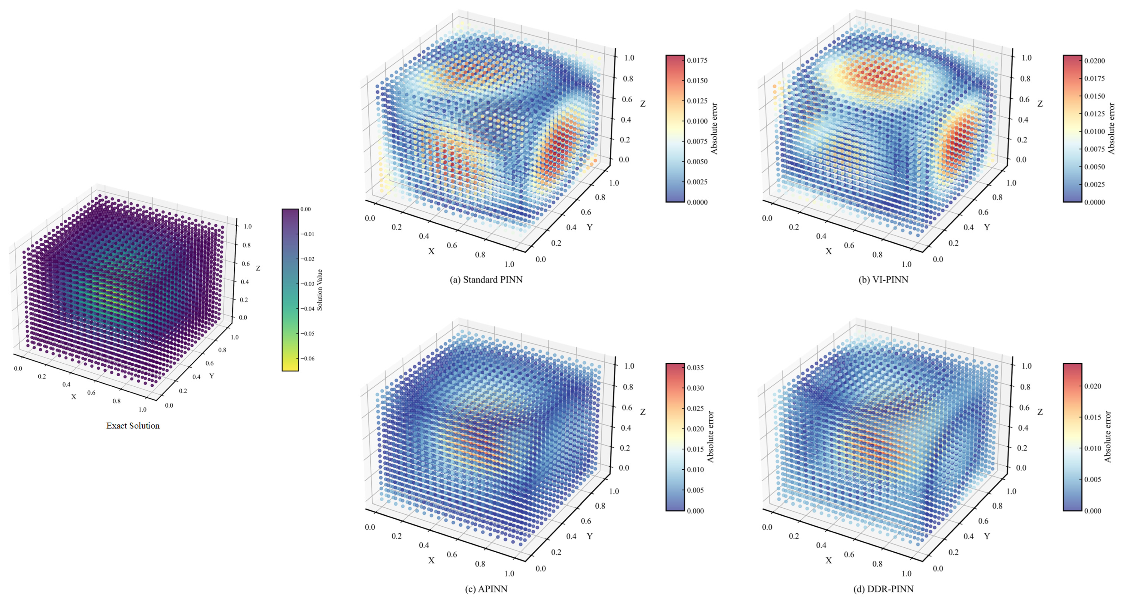
Figure 13 presents the exact solution of the 3D wave equation at the intermediate time step (t = $\sqrt{2}/2$). It can be clearly observed that there are relatively high disturbance values in the interior domain, while the boundary values are zero, which is consistent with the Dirichlet boundary conditions. The APINN achieves the highest accuracy in the boundary solution, followed by the DDR-PINN. The maximum absolute error 0.035 occurs in the APINN, indicating that the APINN focuses on improving boundary accuracy but lacks sufficient learning for the interior domain, guided by a multi-task learning mechanism. Among PINNs, the DDR-PINN achieves the optimal balance solution accuracy between the interior and boundary domains, thus achieving higher accuracy on the test set.

Figure 13. The absolute error of PINN solutions for the 3D wave equation at the intermediate time step (t = √2/2): (a) standard PINN solution absolute error, (b) VI-PINN solution absolute error, (c) APINN solution absolute error, (d) DDR-PINN solution absolute error.

5. Discussion

In this section, we discuss the improvement, limitation and future work of the DDR-PINN.

• The DDR-PINN directly reveals the primary part affecting convergence from the interior domain, boundary domain, and initial domain in the process of solving various dimension PDEs, explicitly providing a useful reference for focusing on domains characterized by high residuals and strong variations.
• As research on PINNs advances, the algorithm complexity and the number of parameters deserve more attention. The DDR-PINN offers a viable pathway for solving high-order PDEs with complex geometric boundaries with enhanced solution accuracy, while the number of trainable parameters are regulated effectively.
• The limitation lies in the performance of boundary value solving. Due to the oscillatory nature of the wave equation, gradients undergo drastic variations in the transition region between the interior domain and the boundary domain. Although we employed the hyperbolic tangent function for optimization, relatively large errors still persist in the 2D wave equation, which indicates that the DDR-PINN still has room for improvement in handling variable boundary conditions.

In summary, the DDR-PINN demonstrates distinct advantages specifically in scenarios characterized by strong differences between boundary conditions and governing equations with specific parameter requirements, whereas the drastic fluctuations in gradients undermine the stability of the solution process. In future work, we will attempt to further explore the latent space correlation between gradients and solution functions. By establishing a bidirectional mapping relationship between partial derivatives and spatiotemporal coordinates, the convergence of PINNs would be faster and more stable. Furthermore, the development of lightweight and modularized reweighted PINNs will also constitute a key direction for our subsequent investigations.

6. Conclusions

This study proposes the DDR-PINN, which innovatively integrates residual information and solution gradients for reweighting, guiding the PINN to focus on domains with large residuals and intense fluctuations. Then, the DDR-PINN is applied to solve heat equations and wave equations in six inhomogeneous PDEs, with Dirichlet and Neumann boundary conditions. The main conclusions of this paper are as follows:

• DDR exhibits excellent generalization capability, achieving an MSE that outperforms other benchmark PINNs by 40.00%, 29.58%, and 52.10%, with the dimension from 1D to 3D when solving the inhomogeneous heat equation. For the inhomogeneous wave equation, it outperforms other benchmark PINNs by 66.96, 9.36%, and 1.30%.
• Incorporating gradient-based reweighting proves to be effective in alleviating conflicts among loss terms. Across all experiments, the DDR-PINN exhibits noticeably faster convergence, together with a more stable fluctuation magnitude and frequency than other PINNs.
• The DDR-PINN fully leverages the inherent automatic differentiation and residual mechanisms of the PINN framework, without additional hyperparameters for tuning, while exerting favorable control over the volume of trainable parameters.

This study also reveals a significant correlation between loss term conflicts and learning rate adjustments during PDE solving with PINNs, and that the appropriate addition of nonlinear transformations in PINNs exerts a positive effect. This provides directions for PINN-related work, and we will further explore the use of learning rates and gradient-based methods to address loss term conflicts in PINNs.

References

- Gong, Y.; Liu, G.; Xue, Y.; Li, R.; Meng, L. A Survey on Dataset Quality in Machine Learning. Inf. Softw. Technol. 2023, 162, 107268. [Google Scholar] [CrossRef] [Scilit]
- Han, H.; Wu, Y.; Wang, J.; Han, A. Interpretable Machine Learning Assessment. Neurocomputing 2023, 561, 126891. [Google Scholar] [CrossRef] [Scilit]
- Wu, Y.; Sicard, B.; Gadsden, S.A. Physics-Informed Machine Learning: A Comprehensive Review on Applications in Anomaly Detection and Condition Monitoring. Expert Syst. Appl. 2024, 255, 124678. [Google Scholar] [CrossRef] [Scilit]
- Karniadakis, G.E.; Kevrekidis, I.G.; Lu, L.; Perdikaris, P.; Wang, S.; Yang, L. Physics-Informed Machine Learning. Nat. Rev. Phys. 2021, 3, 422–440. [Google Scholar] [CrossRef] [Scilit]
- Meng, C.; Griesemer, S.; Cao, D.; Seo, S.; Liu, Y. When Physics Meets Machine Learning: A Survey of Physics-Informed Machine Learning. Mach. Learn. Comput. Sci. Eng. 2025, 1, 20. [Google Scholar] [CrossRef] [Scilit]
- Luo, K.; Zhao, J.; Wang, Y.; Li, J.; Wen, J.; Liang, J.; Soekmadji, H.; Liao, S. Physics-Informed Neural Networks for PDE Problems: A Comprehensive Review. Artif. Intell. Rev. 2025, 58, 323. [Google Scholar] [CrossRef] [Scilit]
- Song, Y.; Zhang, A. From Black Box to Physically Interpretable: Trustworthy Computing for AI-Driven Decision-Making and Control. J. Autom. Intell. 2025. [Google Scholar] [CrossRef] [Scilit]
- Oneto, L.; Ridella, S.; Anguita, D. Informed Machine Learning: Excess Risk and Generalization. Neurocomputing 2025, 646, 130521. [Google Scholar] [CrossRef] [Scilit]
- Vairo, T.; Cademartori, D.; Clematis, D.; Asensio, A.M.; Barbucci, A.; Carpanese, M.P. A Physics-Informed Neural Network (PINN) Predicting the Performance of Air Electrodes for Solid Oxide Cells: A Pilot-Scale Demonstration on Four Microstructures. Int. J. Hydrogen Energy 2025, 176, 151322. [Google Scholar] [CrossRef] [Scilit]
- Zhou, Y.; Song, H. Data-Driven Enhanced Rough Contact Mechanics: PINN Estimation of Gap Distribution across Length Scales for Partial Contacts. Tribol. Int. 2026, 214, 111100. [Google Scholar] [CrossRef] [Scilit]
- Luo, D.; Mo, H.; Li, Q.; Jin, X. Solution of Stress and Deformation Field and Inversion of Material Parameter for Gravity Dams Based on Physics-Informed Neural Networks. J. Comput. Sci. 2025, 89, 102613. [Google Scholar] [CrossRef] [Scilit]
- Roozbahani, M.S.; Soltani, M.; Sayah, M.R.; Shamloo, A.; Hannani, S.K. Design and Optimization of Heat Transfer Channel Using Physics-Informed Neural Networks (PINN) and Deep Gaussian Processes. Therm. Sci. Eng. Prog. 2025, 66, 104012. [Google Scholar] [CrossRef] [Scilit]
- Kütük, M.; Yücel, H. Energy Dissipation Preserving Physics Informed Neural Network for Allen–Cahn Equations. J. Comput. Sci. 2025, 87, 102577. [Google Scholar] [CrossRef] [Scilit]
- Chen, J.; Shi, Y.; Yu, Y. A C-PINN Method for Structural Seismic Response Modeling. Structures 2025, 82, 110422. [Google Scholar] [CrossRef] [Scilit]
- Sundar, R.; Lucor, D.; Sarkar, S. Sequential Learning Based PINNs to Overcome Temporal Domain Complexities in Unsteady Flow Past Flapping Wings. J. Fluids Struct. 2025, 139, 104421. [Google Scholar] [CrossRef] [Scilit]
- Zhou, X.; Li, Z.; Liu, X.; Wang, Y.; Liang, N.; Zhong, Z. Physics-Informed Neural Network (PINN) for Predicting the Temperature Field in High Geothermal Tunnels. Tunn. Undergr. Space Technol. 2026, 169, 107265. [Google Scholar] [CrossRef] [Scilit]
- Wang, Y.; Qiu, X.; Pei, Q.; Wang, J.; Zhang, P.; Bai, X. FAMAW-PINN: A Physics-Informed Neural Network Integrating Adaptive Loss Weighting with Firefly-Inspired Adaptive Point Movement. J. Comput. Phys. 2025, 542, 114363. [Google Scholar] [CrossRef] [Scilit]
- Wang, S.; Yu, X.; Perdikaris, P. When and Why PINNs Fail to Train: A Neural Tangent Kernel Perspective. J. Comput. Phys. 2022, 449, 110768. [Google Scholar] [CrossRef] [Scilit]
- Cao, F.; Guo, X.; Dong, X.; Yuan, D. WbPINN: Weight Balanced Physics-Informed Neural Networks for Multi-Objective Learning. Appl. Soft Comput. 2025, 170, 112632. [Google Scholar] [CrossRef] [Scilit]
- Yan, D.; He, L. DP-PINN+: A Dual-Phase PINN Learning with Automated Phase Division. J. Comput. Sci. 2025, 90, 102637. [Google Scholar] [CrossRef] [Scilit]
- Feng, W.; Hu, M.; Huang, R.; Tang, C.; Huang, S.; Lv, J. DSAIS-PINN: Dynamic Seeds Allocation Importance Sampling for Physics-Informed Neural Networks. Neurocomputing 2025, 648, 130578. [Google Scholar] [CrossRef] [Scilit]
- Jiang, F.; Hou, X.; Ye, J.; Xia, M. Deeper-PINNs: Unlocking the Power of Deep Physics-Informed Neural Networks. Appl. Soft Comput. 2025, 185, 114048. [Google Scholar] [CrossRef] [Scilit]
- Fan, M.-H.; Zhao, J.-H.; Ding, L.; Ma, X.-Y.; Fu, R.-L. Predicting Nonlinear Dynamic Systems by Causal Physics-Informed Neural Networks with ResNet Blocks. Neurocomputing 2025, 656, 131589. [Google Scholar] [CrossRef] [Scilit]
- Yang, T.; Qian, Z.; Hang, N.; Liu, M. S-PINN: Stabilized Physics-Informed Neural Networks for Alleviating Barriers between Multi-Level Co-Optimization. Comput. Methods Appl. Mech. Eng. 2025, 447, 118348. [Google Scholar] [CrossRef] [Scilit]
- Shan, B.; Li, Y.; Huang, S.-J. VI-PINNs: Variance-Involved Physics-Informed Neural Networks for Fast and Accurate Prediction of Partial Differential Equations. Neurocomputing 2025, 623, 129360. [Google Scholar] [CrossRef] [Scilit]
- Gao, B.; Yao, R.; Li, Y. Physics-Informed Neural Networks with Adaptive Loss Weighting Algorithm for Solving Partial Differential Equations. Comput. Math. Appl. 2025, 181, 216–227. [Google Scholar] [CrossRef] [Scilit]
- Li, W.; Wang, H.; Guan, H.; Zhou, R.; Zhang, C.; Tao, D. AdaPW: An Adaptive Point-Weighting Method for Training Physics-Informed Neural Networks. Comput. Math. Appl. 2025, 198, 255–273. [Google Scholar] [CrossRef] [Scilit]
- Chen, W.; Howard, A.A.; Stinis, P. Self-Adaptive Weights Based on Balanced Residual Decay Rate for Physics-Informed Neural Networks and Deep Operator Networks. J. Comput. Phys. 2025, 542, 114226. [Google Scholar] [CrossRef] [Scilit]
- Zhang, J.; Zhao, Y.; Tang, Y. Adaptive Loss Weighting Auxiliary Output FPINNs for Solving Fractional Partial Integro-Differential Equations. Phys. D Nonlinear Phenom. 2024, 460, 134066. [Google Scholar] [CrossRef] [Scilit]
- Zhang, L.; Liu, Q.; Zhang, R.; Yue, L.; Ding, Z. A Gradient-Variance Weighting Physics-Informed Neural Network for Solving Integer and Fractional Partial Differential Equations. Appl. Sci. 2025, 15, 11137. [Google Scholar] [CrossRef] [Scilit]
- Wang, L.; Lin, Y.; Yan, X.; Shao, Y.; Xu, Z.; Yang, C.; Fan, H.; Xie, Y.; Zheng, C. Modeling of Distributed Parameter Systems Based on Independent Partial Derivative-Physics-Informed Neural Network. Neurocomputing 2025, 642, 130396. [Google Scholar] [CrossRef] [Scilit]
- Raissi, M.; Perdikaris, P.; Karniadakis, G.E. Physics-Informed Neural Networks: A Deep Learning Framework for Solving Forward and Inverse Problems Involving Nonlinear Partial Differential Equations. J. Comput. Phys. 2019, 378, 686–707. [Google Scholar] [CrossRef] [Scilit]
Disclaimer/Publisher’s Note: The statements, opinions and data contained in all publications are solely those of the individual author(s) and contributor(s) and not of MDPI and/or the editor(s). MDPI and/or the editor(s) disclaim responsibility for any injury to people or property resulting from any ideas, methods, instructions or products referred to in the content. |
© 2026 by the authors. Licensee MDPI, Basel, Switzerland. This article is an open access article distributed under the terms and conditions of the Creative Commons Attribution (CC BY) license.