Generalized Dynamic Security Region of Grid-Following and Grid-Forming Converter-Based Systems by Basin of Attraction Method

Abstract

With renewable integration and zero-carbon microgrids achieving 100% penetration, converter-dominated systems exhibit millisecond-timescale transient synchronization, which challenges existing physical cognitive methods and cognitive methodology with the synchronous generator (SG). In this paper, in order to quantificationally analyze the transient synchronization, a unified framework has been proposed that combines the generalized participation factor (GPF) method and basin of attraction (BOA) boundary analysis using the manifold approach. According to the GPF and BOA analyses, the fourth-order models are essential for accurate stability quantification, with synchronization controls (PLL, VSG, and droop control) contributing greater than 70% to transient dynamics versus about 20% from power-balance interactions. Further, the dynamic security region (DSR) is redefined by two typologies. Type 1 DSR maps stability in active-power injection space, and Type 2 DSR (generalized DSR) delineates limits in the controllable parameter space. The estimation procedures are proposed for these two types of DSRs by the BOA method. Finally, electromagnetic transient simulations and critical clearing time validation are employed for fidelity verification of models and estimation approaches. To sum up, the proposed novel framework enables systematic DSR estimations for renewable-rich power systems, empowering grid operators to optimize converter-controllable parameters and system operation conditions.

1. Introduction

Under the background of carbon-peaking-neutrality goals and the new-type power system construction, converter-based renewable resources have continuously developed and been utilized, mainly including wind and photovoltaic resources. In China, the installed capacity of renewables has accounted for approximately 42% of the total. At the macroscale, the power system has been gradually governed by converter-based power generation with the continuous increase in renewable generation installation [1,2,3]. At the microscale, there have emerged zero-carbon microgrids (green electricity−hydrogen interaction industrial estate) with a high proportion of renewable energy (wind, solar, and hydrogen energy), even reaching as high as 100% [4]. Different from classical systems dominated by the synchronous generator (SG), the timescale of the transient synchronization has reduced to the millisecond level for renewable-rich systems, which poses a great challenge to stability analyses and stabilization control [5,6].

For converter-based generation, the dynamics have been determined by the control strategies and control parameters of the converter. Synchronization strategies have categorized these systems into two representative types: grid-following (GFL) and grid-forming (GFM) converters [7]. The GFL converters tracked the phase of the voltage at the point of common connection (PCC) by the phase-locked loop (PLL) to achieve synchronization with the grid. The GFM converter achieved synchronization by the virtual synchronous generator (VSG) control, drop control, etc. It has been designed by simulating the dynamic characteristics of the SG. Consequently, modeling and quantitative analyses of the GFL and GFM converter-based systems have been crucial for the transient synchronization stability of renewable-rich power systems.

Over the past century, for the SG, pioneers have constructed fifth-order models (sub-transient, transient, and synchronous dynamics) and third-order models (transient and synchronous dynamics), as well as the swing equation depicting synchronous dynamics for the SG based on the physical dynamic characteristics [8]. Analogized to the SG, the transient reduced-order models of the GFL and GFM converter have been established. For GFL converters, the prevalent 2nd-order model that only considers the dynamics of the PLL has been established by ignoring the voltage control loops and the current control loops. As the 2nd-order model is similar to the swing equation, classical stability analysis methods have been adopted to analyze the transient synchronization mechanism of the GFL converter-based system, such as the energy function and equal area criterion (EAC) [9,10,11,12,13]. However, the equivalent damping of the GFL converters was state-dependent and could be positive or negative during the dynamic processes. The indefinite damping could lead to the analysis results being sometimes conservative and sometimes optimistic. Thus, the energy function and EAC method may be unsuitable for quantification analyses, e.g., the estimation of the basin of attraction (BOA) [14]. For GFM converters, as VSG was designed to simulate the SG’s dynamics, most studies directly omitted the role of other control loops, and thus derived a 2nd-order model, which was completely consistent with the classical swing equation. In this respect, based on the 2nd-order model, the existing research studied the transient synchronization stability of GFM converters by applying classical methods, including the energy function, EAC, phase portraits, etc. [15,16,17,18]. Meanwhile, similarities and differences have been addressed in the transient synchronization between GFM and GFL converters [13,19]. However, the existing studies for the GFM converter have not considered the dynamics of the DC capacitor. What is more, the effects of diverse control loops on transient synchronous behaviors have not yet been fully uncovered. Thus, the widely used 2nd-order equation was overly simplified and cannot fully describe the transient synchronization behaviors of the GFM converter. It was unsuitable for quantification analyses.

Consequently, both GFL converters and GFM converters achieved synchronization through controls, which was fundamentally different from the SG, which was the electromechanical−magnetic conversion apparatus. The timescale separation was not obvious and was greatly affected by the controller’s parameters, and thus, the couplings between each loop cannot be ignored. In addition, the converter includes two synchronous control structures (GFL and GFM), and the outer control strategies were also not the same. Therefore, the physical functions and coupling characteristics of diverse control loops in the converters are still unclear. Reduced-order models have not yet been constructed for quantification analyses of transient synchronization.

Taking the BOA analysis as the foundation and going further, the dynamic security region (DSR) analysis and its estimation have been widely studied and applied in the engineering practice within the SG-dominated power system [20,21,22]. The DSR and BOA can be seen as sister concepts. The BOA depicted the stable region with the state variables. Correspondingly, the DSR was defined in the space composed of the active power of the SG that can be adjusted for power [20]. It has been an important tool for dispatchers to prevent the development and expansion of transient accidents. The DSR of the GFL converter system was preliminarily studied in [23]. Recently, a practical DSR model has been proposed by a physical and data-driven method, which was focused on the SG-dominated power grid [24]. Therefore, the literature has paid attention to transient synchronization mechanism analysis, while the quantification analyses and DSR estimation have been overlooked for converter-based systems.

To overcome these obstacles, the DSRs for renewable-rich power systems have been enriched and redefined by the BOA analysis. The main contributions and novelties of this article can be summarized as follows:

(1) Unified reduced-order modeling. For GFL and GFM converter-based systems, the reduced-order models have been uniformly established by the generalized participation factor and the manifold methods. Analyses reveal that the synchronization control loops, including the PLL, VSG, and droop control, govern transient synchronization as the primary mechanism, with power-balance dynamics acting as the secondary dominant factor.

(2) Boundaries of the BOA approximation. The boundaries of BOAs are approximated via the manifold method. Based on the BOA analyses, model fidelity is validated through cross-verification of dominant state variables and BOA analyses. Synthesizing results from BOA geometry, large-signal trajectory, and critical clearing time validation, the 4th-order models are proven essential for precise DSR approximation in both GFL and GFM systems.

(3) DSR concept formulation. Extending classical SG-dominated paradigms, two DSR typologies have been established for renewable-rich power systems. Among them, Type 1 DSR delineates security boundaries in the active power plane of the converter. Meanwhile, Type 2 DSR encapsulates stability limits within the parametric space of dominant control loops (e.g., PLL, VSG, and droop control).

The remainder of this paper is structured as follows. Section 2 establishes the reduced-order models uniformly by generalized participation factor analysis. Then, the BOA analysis is conducted in Section 3, separately for the GFL and GFM converter-based systems. In Section 4, two types of DSR are defined and approximated, and simulation validation is also conducted. Finally, discussions and conclusions are given in Section 5 and Section 6, respectively.

2. Unified Modeling of GFL and GFM Converter Systems Based on CUEP

In the literature, transient synchronous stability can be intuitively formalized as follows: The system maintains stability if its post-fault state trajectory is located within the stability domain of the after-fault system. Thus, transient stability assessment does not require precise estimation of the full stability domain of the stable equilibrium point after a fault, but focuses on the stability boundary of the area near the exit point (the intersection point between the fault trajectory and the boundary of the BOA). Therefore, precise estimation of the stability domain near the CUEP becomes of great importance. Therefore, this section first introduces a generalized participation factor (GPF) analysis method based on the controlling unstable equilibrium point (CUEP). Thus, the reduced-order models can be established both for GFL and GFM converter-based systems, which can be used to estimate boundaries of the BOA and DSR.

2.1. Generalized Participation Factor Analysis Method Based on the Manifold of CUEP

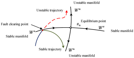
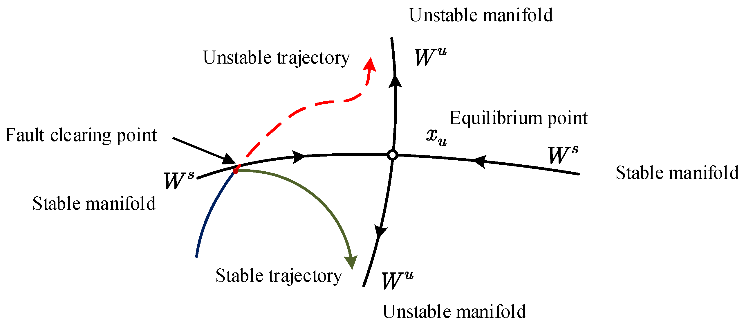
The exit point is located on the CUPE’s stable manifold, where the fault trajectory intersects the stable manifold of CUPE. Crucially, the unstable manifold of the CUEP represents the instability direction and mode of the system, as shown in Figure 1. In Figure 1, the relationships of stable trajectories, unstable trajectories, unstable equilibrium points, and exit points are visualized. In Figure 1, the green solid line represents the stable trajectory while the red dashed line depicts the unstable trajectory. It can be seen that the unstable trajectory is approaching the unstable manifold of the CUEP. Thus, the unstable manifold at CUEP determines the instability mode of the system. Although the unstable manifold does not describe the exact post-fault trajectory, the during-fault trajectory approaches it as time goes by. By studying the local manifolds of the nonlinear system linearized at the CUEP, the dominant transient stability behaviors of the system can be revealed. Consequently, state variables that exhibit strong correlation with this instability mode (the unstable manifold) can be identified as key variables and control loops governing the system’s transient synchronization dynamics.

Figure 1. Schematic showing the stable/unstable trajectories and CUEP’s stable/unstable manifolds. The arrow indicates the direction of the trajectory’s change over time.

The linear form of a general dynamic system at CUEP can be obtained by linearizing, namely, the following:

$${\displaystyle \frac{\mathrm{d}\Delta \mathbf{x}}{\mathrm{d}t}}=\mathbf{J}\Delta \mathbf{x}$$

(1)

where J is the Jacobian matrix. d(·)/dt denotes the differentiating operator. Δ denotes the Laplace operator. The right eigenvector z and left eigenvector y^T of the unique unstable eigenvalue μ can be derived as:

$$\mathbf{J}\mathbf{z}=\mu \mathbf{z}, {\mathbf{y}}^{\mathrm{T}}\mathbf{J}=\mu {\mathbf{y}}^{\mathrm{T}}$$

(2)

In this respect, the generalized participation factor of each state variable (p_k) on the unstable eigenvalue can be defined as:

$$p_k={\displaystyle \frac{y_k{z}_k}{\mathbf{y}\mathbf{z}}}$$

(3)

where y_k and z_k separately represent the left and right eigenvectors associated with the unique unstable eigenvalue μ.

From the physical interpretation of the generalized participation factor, the magnitude of each state variable’s participation factor for the positive eigenvalue directly quantifies its contribution to the unstable manifold, thereby indicating its role in system instability. By evaluating the generalized participation factor of the unstable equilibrium point, we can identify state variables or control loops critical to transient synchronization. Correspondingly, reduced-order models can be further constructed for quantitative analyses of the transient synchronization stability. While the computational procedures for the generalized and classical participation factors share methodological commonalities, three fundamental distinctions exist. Firstly, the classical participation factor derives from the stable equilibrium point, whereas the generalized participation factor operates at the CUPE. Secondly, for the physical interpretation, the classical participation factor measures the contribution of each state variable to the stability manifold of the stable equilibrium point. The generalized participation factor quantifies the contribution of each state variable to the unstable manifold. Thirdly, the classical participation factor analysis (modal analysis) addresses the small-signal stability, while the proposed generalized participation factor targets the large-signal stability. To sum up, the proposed CUEP-based method fundamentally differs in application and physical interpretation. As the computation procedures of the generalized and classical participation factors are the same, the sensitivity of the proposed generalized participation factors algorithm meets the requirements.

Following this, the proposed method is applied to determine dominant control loops and establish mathematical equations for the GFL and GFM converter-based systems under different control structures. For the GFL converters, the voltage control and active/reactive power control are analyzed. For the GFM converters, the VSG and droop control are mainly considered. It should be emphasized that hierarchical reduced-order models for SGs have been derived using the singular perturbation theory, which is valid based on the fact of timescale separation. For converter-based apparatuses, the timescales of various control loops depend on their PI gains, which leads to deep couplings between different controls. The couplings invalidate the timescale separation prerequisite, rendering the singular perturbation theory inapplicable for converter stability analysis.

2.2. Reduced-Order Model of the GFL Converter

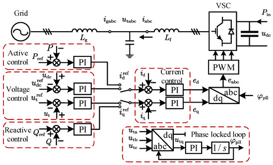
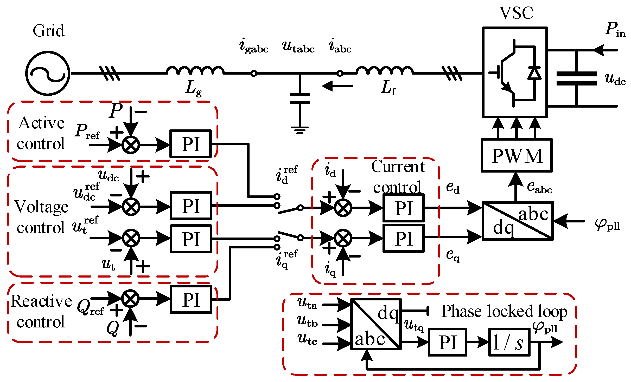
The topology of the GFL converter system and its controls are depicted in Figure 2. On the DC side, the active power P_m generated by the machine-side converter is transmitted to the grid-side VSC through capacitor C. On the AC side, the grid-side converter is connected to the grid through the filter inductor L_f, filter capacitor C_f, and grid inductor L_g. Within PLL control, the q-axis component U_tq of the terminal voltage U_t is always zero, ensuring that the d-axis of the dq rotating coordinate system is always in the same direction as the terminal voltage U_t. The converter on the grid side is mainly composed of control loops such as voltage/power (outer loops) control, alternating current (inner loop) control, and PLL control. According to the functions and targets of outer control loops, they can mainly be divided into two categories: the voltage control and power control. The voltage outer loop controls the input terminal voltage and DC voltage, while the power outer loop controls the active and reactive power input. The point is that they both output active and reactive current references, namely $i_{\mathrm{d}}^{\mathrm{ref}}$ and $i_{\mathrm{q}}^{\mathrm{ref}}$. The alternating current control (ACC) controls the output current of the converter according to the given active and reactive current references, outputs the modulated voltages e_d and e_q, and then generates the trigger signal through the abc coordinate transformation and modulation.

Figure 2. Schematic showing the GFL converter-based system and its controls.

For the GFL converter with voltage outer loop control, the nonlinear model incorporates terminal voltage control (TVC), DC capacitor dynamics, direct voltage control (DVC), PLL, ACC, and line capacitor and inductor dynamics. Select the integrator output of all PI controllers and the DC voltage u_dc as state variables, and the state-space model can be obtained, namely, as follows:

$$\left\{\begin{array}{l}\dot{\phi }=x_{\mathrm{pll}}+k_{\mathrm{ppll}}{u}_{\mathrm{tq}},{\dot{x}}_{\mathrm{pll}}=k_{\mathrm{ipll}}{u}_{\mathrm{tq}}\\ {\dot{x}}_{\mathrm{dvc}}=k_{\mathrm{idvc}}(u_{\mathrm{dc}}-u_{\mathrm{dc}}^{\mathrm{ref}}),{\dot{u}}_{\mathrm{dc}}=(P_{\mathrm{in}}-P_{\mathrm{e}})/(C_{\mathrm{dc}}{u}_{\mathrm{dc}})\\ {\dot{x}}_{\mathrm{tvc}}=k_{\mathrm{itvc}}(u_{\mathrm{td}}-u_{\mathrm{td}}^{\mathrm{ref}})\\ {\dot{x}}_{\mathrm{acc}1}=k_{\mathrm{iacc}}(i_{\mathrm{d}}^{\mathrm{ref}}-i_{\mathrm{d}}),{\dot{x}}_{\mathrm{acc}2}=k_{\mathrm{iacc}}(i_{\mathrm{q}}^{\mathrm{ref}}-i_{\mathrm{q}})\end{array}\right.$$

(4)

In Equation (4), φ and x_pll respectively represent the angle and frequency output of the PLL control; x_dvc and x_tvc respectively represent DVC and TVC integrator outputs; x_acc1,2 represent the d- and q-axis controller integrator outputs of ACC. P_in and P_e separately denote the input and electromagnetic powers; C_dc denotes the DC-side capacitance; u_dc and ${\mathrm{u}}_{\mathrm{dc}}^{\mathrm{ref}}$ separately denote the DC-side voltage and its reference. u_td and $u_{\mathrm{td}}^{\mathrm{ref}}$ separately denote the d-axis component and its reference of the terminal voltage U_t; u_tq denotes the q-axis component of the terminal voltage U_t; i_d and i_q separately denote the d-axis and q-axis components of the line current i_abc. For PI gains, k_ppll and k_ipll separately denote PI gains of the PLL, k_pdvc and k_idvc separately denote PI gains of the DVC, k_ptvc and k_itvc separately denote PI gains of the terminal voltage control (TVC), and k_pacc and k_iacc separately denote PI gains of the ACC. The dynamics of the line capacitor and inductor can be expressed in the matrix form, namely, as follows:

$$\left\{\begin{array}{l}{\displaystyle \frac{\mathrm{d}}{\mathrm{d}t}}\left[\begin{array}{c}{i}_{\mathrm{d}}\\ i_{\mathrm{q}}\end{array}\right]=\left[\begin{array}{cc}{\displaystyle \frac{{\omega }_0}{L_{\mathrm{f}}}}& \\ & {\displaystyle \frac{{\omega }_0}{L_{\mathrm{f}}}}\end{array}\right]\left[\begin{array}{c}{e}_{\mathrm{d}}\\ e_{\mathrm{q}}\end{array}\right]-\left[\begin{array}{cc}1& \\ & 1\end{array}\right]\left[\begin{array}{c}{u}_{\mathrm{td}}\\ u_{\mathrm{tq}}\end{array}\right]+\left[\begin{array}{cc}& {\omega }_0+\omega \\ -({\omega }_0+\omega )& \end{array}\right]\left[\begin{array}{c}{i}_{\mathrm{d}}\\ i_{\mathrm{q}}\end{array}\right]\\ {\displaystyle \frac{\mathrm{d}}{\mathrm{d}t}}\left[\begin{array}{c}{u}_{\mathrm{td}}\\ u_{\mathrm{tq}}\end{array}\right]=\left[\begin{array}{cc}{\displaystyle \frac{{\omega }_0}{C_{\mathrm{f}}}}& \\ & {\displaystyle \frac{{\omega }_0}{C_{\mathrm{f}}}}\end{array}\right]\left[\begin{array}{c}{i}_{\mathrm{d}}\\ i_{\mathrm{q}}\end{array}\right]-\left[\begin{array}{cc}1& \\ & 1\end{array}\right]\left[\begin{array}{c}{i}_{\mathrm{gd}}\\ i_{\mathrm{gq}}\end{array}\right]+\left[\begin{array}{cc}& {\omega }_0+\omega \\ -({\omega }_0+\omega )& \end{array}\right]\left[\begin{array}{c}{u}_{\mathrm{td}}\\ u_{\mathrm{tq}}\end{array}\right]\\ {\displaystyle \frac{\mathrm{d}}{\mathrm{d}t}}\left[\begin{array}{c}{i}_{\mathrm{gd}}\\ i_{\mathrm{gq}}\end{array}\right]=\left[\begin{array}{cc}{\displaystyle \frac{{\omega }_0}{L_{\mathrm{g}}}}& \\ & {\displaystyle \frac{{\omega }_0}{L_{\mathrm{g}}}}\end{array}\right]\left[\begin{array}{c}{u}_{\mathrm{td}}\\ u_{\mathrm{tq}}\end{array}\right]-\left[\begin{array}{cc}1& \\ & 1\end{array}\right]\left[\begin{array}{c}{u}_{\mathrm{gd}}\\ u_{\mathrm{gq}}\end{array}\right]+\left[\begin{array}{cc}& {\omega }_0+\omega \\ -({\omega }_0+\omega )& \end{array}\right]\left[\begin{array}{c}{i}_{\mathrm{gd}}\\ i_{\mathrm{gq}}\end{array}\right]\end{array}\right.$$

(5)

where i_d,q and i_gd,q represent the d- and q-axis components of the line current respectively; u_td,q represents the d- and q-axis components of the voltage at the PCC point. u_gd,q represents the d- and q-axis components of the grid voltage. The algebraic variables in Equation (5) satisfy:

$$\left\{\begin{array}{l}{i}_{\mathrm{d}}^{\mathrm{ref}}=k_{\mathrm{pdvc}}(u_{\mathrm{dc}}-u_{\mathrm{dc}}^{\mathrm{ref}})+x_{\mathrm{dvc}},i_{\mathrm{q}}^{\mathrm{ref}}=k_{\mathrm{ptvc}}(u_{\mathrm{td}}-u_{\mathrm{td}}^{\mathrm{ref}})+x_{\mathrm{tvc}}\\ e_{\mathrm{d}}=k_{\mathrm{pacc}}(i_{\mathrm{d}}^{\mathrm{ref}}-i_{\mathrm{d}})+x_{\mathrm{acc}1},e_{\mathrm{q}}=k_{\mathrm{pacc}}(i_{\mathrm{q}}^{\mathrm{ref}}-i_{\mathrm{q}})+x_{\mathrm{acc}2}\end{array}\right.$$

(6)

Furthermore, solving the steady-state algebraic equations derived from setting the right-hand sides of Equations (4) and (5) to zero yields two equilibrium points. Based on the theory of small-signal stability analysis, the equilibrium point x₀ with phase φ₀ between 0 and π/2 is the stable equilibrium point (all eigenvalues are located in the left half-plane), while x_u with phase between π/2 and π is the unstable equilibrium point (there exist right half-plane eigenvalues). The analytical formulations of equilibrium points are provided in Appendix A. Critically, for a single converter system, only one unstable equilibrium point (UEP) exists, consequently serving as the CUEP. In multi-converter systems, there exists multiple unstable equilibrium points associated with diverse instability modes. In this respect, the CUEP can be determined by combining the fault trajectories and BOA.

Following this, the dominant control loops of the GFL converter-based system with the voltage outer loop control are analyzed by using the proposed generalized participation factor method. As similar timescales (associated with the bandwidth) of different control loops could deepen the couplings of dynamic behaviors, the bandwidths of control loops are changed to make the cases general. Thus, without loss of generality, multiple groups of parameters are selected under various conditions. The parameter sets spanning diverse operating conditions have been evaluated, establishing conclusions with demonstrated robustness and applicability. Taking case 1 as the benchmark, case 2 increases the grid inductance L_g for a weak grid. Cases 3 and 4 respectively reduce and increase the PI parameters of the PLL, that is, decrease and increase the PLL bandwidth. Case 5 reduces the PI parameters of ACC, namely, decreasing the ACC bandwidth. Correspondingly, it can deepen the couplings between the ACC and other controls. Case 6 increases the PI parameters of TVC. Similarly, it can deepen the couplings between the TVC and ACC. The specific parameters can be found in Appendix B.

Table 1 shows generalized participation factors of state variables relative to the unstable manifold under six cases. Dominance of the state variable can be revealed by combining these cases. In case 1, PLL states (φ and x_pll) and power-balance states (x_dvc and u_dc) collectively contribute 93% (0.63 + 0.30) of system dynamics, while the sum of the other state quantities is only 0.07. This pattern persists in Cases 2–6 (rows 3–7), where the six-case average (row 8) confirms 90% dominance by PLL synchronization and power-balance dynamics (DC capacitor plus DVC). Furthermore, the generalized participation factor of the PLL is around 0.6, and the participation factor of the power-balancing stage is around 0.3. Consequently, PLL dynamics primarily govern transient synchronization stability, while power-balance dynamics act as a secondary yet non-negligible contributor. Crucially, control loop dominance constitutes a context-dependent concept, analogous to engineering thresholds for small-signal perturbations (typically ±10% of nominal values). When the generalized participation factor exhibits order-of-magnitude disparities (e.g., 90% vs. 10%), the state variables exceeding 90% generalized participation factor dominance dictate the system’s instability dynamic behaviors.

Table 1. Generalized participation factors of the GFL converter with voltage outer control loops.

No.	PLL States	Power-Balance States	Sum	Sum of the Rest
No. 1	0.63	0.30	0.93	0.07
No. 2	0.62	0.29	0.91	0.09
No. 3	0.56	0.38	0.94	0.06
No. 4	0.68	0.22	0.90	0.10
No. 5	0.57	0.24	0.81	0.19
No. 6	0.63	0.32	0.95	0.05
Mean value	0.62	0.29	0.91	0.09

Therefore, control loop dominance can be ranked by generalized participation factor values of different state variables. State variables φ and x_pll are associated with dynamics of the PLL, and x_dvc and u_dc are associated with dynamics of the DVC and DC capacitor. Meanwhile, x_dvc is associated with dynamics of the TVC. State variables x_acc1,2 are associated with dynamics of the ACC. Thus, two models can be derived. One is a 4th-order equation with higher precision considering DVC, capacitance dynamics, and PLL, as follows:

$$\left\{\begin{array}{l}\dot{\phi }=x_{\mathrm{pll}}+k_{\mathrm{p},\mathrm{pll}}{u}_{\mathrm{tq}}\\ {\dot{x}}_{\mathrm{pll}}=k_{\mathrm{ipll}}{u}_{\mathrm{tq}}\\ {\dot{u}}_{\mathrm{dc}}=(P_{\mathrm{in}}-P_{\mathrm{e}})/(C_{\mathrm{dc}}{u}_{\mathrm{dc}})\\ {\dot{x}}_{\mathrm{dvc}}=k_{\mathrm{idvc}}(u_{\mathrm{dc}}-u_{\mathrm{dc}}^{\mathrm{ref}})\end{array}\right.$$

(7)

where φ and x_pll respectively represent the angle and frequency outputs of the PLL; x_dvc and x_tvc respectively represent DVC and TVC integrator outputs; P_in and P_e separately denote the input and electromagnetic powers. u_dc and ${\mathrm{u}}_{\mathrm{dc}}^{\mathrm{ref}}$ separately denote the DC-side voltage and its reference. k_idvc denotes the integral gain of the DVC. u_tq denotes the q-axis component of the terminal voltage U_t. In Equation (7), algebraic variables satisfy:

$$\left\{\begin{array}{l}{i}_{\mathrm{dref}}=k_{\mathrm{p},\mathrm{dvc}}(u_{\mathrm{dc}}-u_{\mathrm{dcref}})+x_{\mathrm{dvc}}\\ u_{\mathrm{tq}}={\displaystyle \frac{{\omega }_0{L}_{\mathrm{g}}{i}_{\mathrm{d}}^{\mathrm{ref}}-U_{\mathrm{g}}\sin \phi +x_{\mathrm{pll}}{L}_{\mathrm{g}}{i}_{\mathrm{d}}^{\mathrm{ref}}}{(1-k_{\mathrm{p},\mathrm{pll}}{L}_{\mathrm{g}}{i}_{\mathrm{d}}^{\mathrm{ref}}-{\omega }_0{L}_{\mathrm{g}}{\omega }_0{C}_{\mathrm{f}})}}\\ u_{\mathrm{td}}=1\\ P_{\mathrm{e}}=u_{\mathrm{td}}{i}_{\mathrm{d}}^{\mathrm{ref}}+u_{\mathrm{tq}}{i}_{\mathrm{q}}^{\mathrm{ref}}\end{array}\right.$$

(8)

For the simpler equation, it only considers PLL dynamics, namely, the following:

$$\left\{\begin{array}{l}\dot{\phi }={\displaystyle \frac{k_{\mathrm{ppll}}({\omega }_0{L}_{\mathrm{g}}{i}_{\mathrm{d}}^{\mathrm{ref}}-U_{\mathrm{g}}\sin \phi +x_{\mathrm{pll}}{L}_{\mathrm{g}}{i}_{\mathrm{d}}^{\mathrm{ref}})}{1-k_{\mathrm{ppll}}{L}_{\mathrm{g}}{i}_{\mathrm{d}}^{\mathrm{ref}}-{\omega }_0{L}_{\mathrm{g}}{\omega }_0{C}_{\mathrm{f}}}}+x_{\mathrm{pll}}\\ {\dot{x}}_{\mathrm{pll}}={\displaystyle \frac{k_{\mathrm{ipll}}({\omega }_0{L}_{\mathrm{g}}{i}_{\mathrm{d}}^{\mathrm{ref}}-U_{\mathrm{g}}\sin \phi +x_{\mathrm{pll}}{L}_{\mathrm{g}}{i}_{\mathrm{d}}^{\mathrm{ref}})}{1-k_{\mathrm{ppll}}{L}_{\mathrm{g}}{i}_{\mathrm{d}}^{\mathrm{ref}}-{\omega }_0{L}_{\mathrm{g}}{\omega }_0{C}_{\mathrm{f}}}}\end{array}\right.$$

(9)

where φ and x_pll respectively represent the angle and frequency outputs of the PLL. C_f denotes the filter capacitance, ω₀ denotes the angular speed of the power frequency, and equals 2π × 50 Hz. Compared with Equation (7), Equation (9) offers significant advantages over Equation (7) in both simplicity and physical interpretability. Its structure has certain similarities with the swing equation of the SG, which has been addressed in the literature [9,10,11,12,13].

For the GFL converter with power controls, the state-space model considers the dynamics of the active power control (APC), reactive power control (RPC), PLL, ACC, and LCL filter. The controller dynamics are described by Equation (10), and the line dynamics are the same as those in Equation (5):

$$\left\{\begin{array}{l}\dot{\phi }=x_{\mathrm{pll}}+k_{\mathrm{p},\mathrm{pll}}{u}_{\mathrm{tq}},{\dot{x}}_{\mathrm{pll}}=k_{\mathrm{i},\mathrm{pll}}{u}_{\mathrm{tq}}\\ {\dot{x}}_{\mathrm{apc}}=k_{\mathrm{i},\mathrm{apc}}(P_{\mathrm{ref}}-P_{\mathrm{e}}),{\dot{x}}_{\mathrm{rpc}}=k_{\mathrm{i},\mathrm{rpc}}(Q_{\mathrm{ref}}-Q_{\mathrm{e}})\\ {\dot{x}}_{\mathrm{acc}1}=k_{\mathrm{i},\mathrm{acc}}(i_{\mathrm{d}}^{\mathrm{ref}}-i_{\mathrm{d}}),{\dot{x}}_{\mathrm{acc}2}=k_{\mathrm{i},\mathrm{acc}}(i_{\mathrm{q}}^{\mathrm{ref}}-i_{\mathrm{q}})\end{array}\right.$$

(10)

where the x_apc and x_rpc are the integrator outputs of APC and RPC, respectively. The algebraic equation is similar to Equation (6).

Without losing generality, six groups of parameters under different conditions are examined to evaluate robustness by changing bandwidths of control loops. Case 1 serves as the baseline configuration, while case 2 increases the grid inductance L_g for the weak grid. Cases 3 and 4 respectively decrease and increase PI gains for the APC to weaken or deepen the couplings between the APC and other controls. Case 5 reduces the PI gains for RPC. Case 6 lowers ACC bandwidth through PI gain reduction to deepen couplings between the ACC and other controls. As shown in Table 2, the generalized participation factors of PLL states (φ and x_pll) collectively reach 0.95, whereas power loop states (x_apc and x_rpc) contribute merely 0.02. Crucially, across parameter perturbations in Cases 2–6, for the GFL VSC under the power outer loop control, the PLL dynamic participation factor accounts for about 90% of all dynamics, demonstrating that synchronization mechanisms governed by PLL dominate transient instability regardless of control parameter variations or grid impedance changes. Therefore, for the GFL VSC controlled by the power loop, the 2nd model that only considers the dynamics of the PLL can fully describe its dynamics. The equation is completely consistent with Equation (9).

Table 2. Generalized participation factors of the GFL converter with power outer control loops.

No.	PLL States	Power-Balance States	Sum	Sum of the Rest
No. 1	0.95	0.02	0.97	0.03
No. 2	0.91	0.04	0.95	0.05
No. 3	0.94	0.03	0.97	0.03
No. 4	0.95	0.01	0.96	0.04
No. 5	0.95	0.03	0.98	0.02
No. 6	0.87	0.02	0.89	0.11
Mean value	0.93	0.03	0.96	0.04

To sum up, for the GFL converter with voltage outer control, the 4th-order model, incorporating both phase synchronization and power-balance dynamics, accurately captures the original system’s behaviors. In the meantime, the 2nd-order equation isolating the PLL provides basic fidelity for transient analysis. For the power controls, the power-balance dynamics exhibit negligible influence on the transient behaviors (smaller than 5%), while the synchronization loop dominates (greater than 90%). In this respect, the 2nd-order model suffices to characterize system transient synchronous dynamics.

2.3. Reduced-Order Model of the GFM Converter

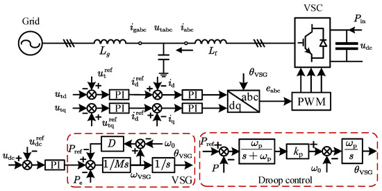
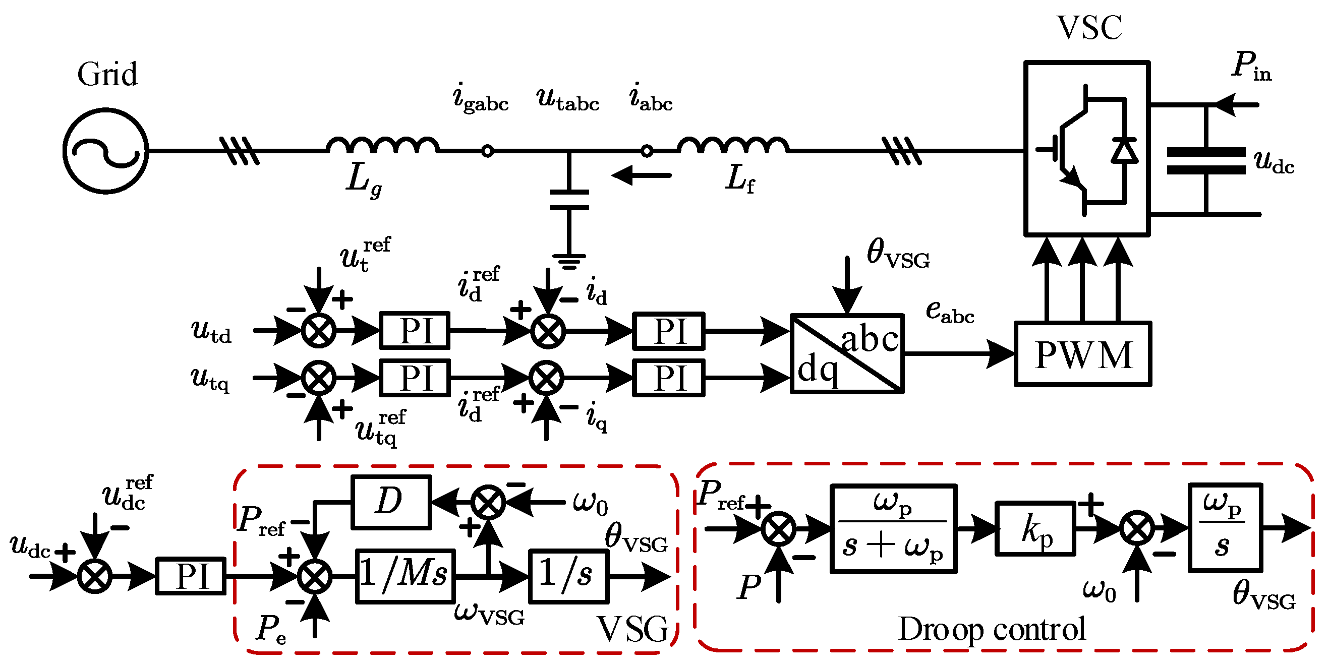
Figure 3 presents the topology and control architecture of the GFM converter-based system, featuring VSG and droop control implementations. Controls of the GFM converter mainly consist of two core branches, including angle generation and internal potential generation. Among them, the angle generation branch is implemented by the VSG, droop controls, and droop controls with the additional filter. For the internal potential generation branch, it typically applies voltage controls.

Figure 3. Schematic showing the GFM converter controlled by VSG and droop control.

Considering the VSG, DVC, and ACC control loops, the dynamics of the converter controller can be described by Equation (11), and the dynamics of the line are the same as Equation (5):

$$\left\{\begin{array}{l}\dot{\delta }=\omega ,M\dot{\omega }=P_{\mathrm{ref}}-P_{\mathrm{e}}-D\omega \\ {\dot{x}}_{\mathrm{dvc}}=k_{\mathrm{i},\mathrm{dvc}}(u_{\mathrm{dc}}-u_{\mathrm{dc}}^{\mathrm{ref}}),{\dot{u}}_{\mathrm{dc}}=(P_{\mathrm{in}}-P_{\mathrm{e}})/(C_{\mathrm{dc}}{u}_{\mathrm{dc}})\\ {\dot{x}}_{\mathrm{tvc}1}=k_{\mathrm{i},\mathrm{tvc}}(u_{\mathrm{td}}^{\mathrm{ref}}-u_{\mathrm{td}}),{\dot{x}}_{\mathrm{tvc}2}=k_{\mathrm{i},\mathrm{tvc}}(u_{\mathrm{tq}}^{\mathrm{ref}}-u_{\mathrm{tq}})\\ {\dot{x}}_{\mathrm{acc}1}=k_{\mathrm{i},\mathrm{acc}}(i_{\mathrm{d}}^{\mathrm{ref}}-i_{\mathrm{d}}),{\dot{x}}_{\mathrm{acc}2}=k_{\mathrm{i},\mathrm{acc}}(i_{\mathrm{q}}^{\mathrm{ref}}-i_{\mathrm{q}})\end{array}\right.$$

(11)

where δ and ω respectively represent the angle and frequency of the VSG output. M and D represent inertia and damping values of the VSG control, and x_tvc1 and x_tvc2 represent the integrator output of the TVC. Algebraic variables in Equation (11) satisfy:

$$\left\{\begin{array}{l}{P}_{\mathrm{ref}}=k_{\mathrm{p},\mathrm{dvc}}(u_{\mathrm{dc}}-u_{\mathrm{dc}}^{\mathrm{ref}})+x_{\mathrm{dvc}},P_{\mathrm{e}}=u_{\mathrm{td}}{i}_{\mathrm{d}}+u_{\mathrm{tq}}{i}_{\mathrm{q}}\\ i_{\mathrm{dref}}=k_{\mathrm{p},\mathrm{tvc}}(u_{\mathrm{td}}-u_{\mathrm{td}}^{\mathrm{ref}})+x_{\mathrm{tvc}1},i_{\mathrm{qref}}=k_{\mathrm{p},\mathrm{tvc}}(u_{\mathrm{tq}}-u_{\mathrm{tq}}^{\mathrm{ref}})+x_{\mathrm{tvc}2}\\ e_{\mathrm{d}}=k_{\mathrm{p},\mathrm{acc}}(i_{\mathrm{d}}^{\mathrm{ref}}-i_{\mathrm{d}})+x_{\mathrm{acc}1},e_{\mathrm{q}}=k_{\mathrm{p},\mathrm{acc}}(i_{\mathrm{q}}^{\mathrm{ref}}-i_{\mathrm{q}})+x_{\mathrm{acc}2}\end{array}\right.$$

(12)

where P_ref is the power reference value output of the DVC.

As shown in Figure 3, the mathematical models for the droop control with first-order low-pass filtering and VSG control exhibit complete equivalence. The structural identity enables parameter mapping through Equation (13), namely, as follows:

$$\left\{\begin{array}{l}M=1/(k_{\mathrm{p}}{\omega }_{\mathrm{p}})\\ D=1/{\omega }_{\mathrm{p}}\end{array}\right.$$

(13)

Similarly, six parameter sets are examined by changing the bandwidths of control loops. Case 1 serves as the baseline for the typical condition. Case 2 increases the grid inductance L_g for the weak grid. Case 3 and Case 4 respectively increase and decrease the VSG inertia constant. Case 5 reduces PI gains of ACC and, accordingly, reduces the ACC bandwidth, which can deepen the couplings between the ACC and other controls. Case 6 increases PI gains of the TVC, namely, accelerating the response speed of the TVC, which can deepen couplings between the TVC and other controls.

As quantified in Table 3 (Case 1, row 2), the generalized participation factors of the VSG states (δ and ω) collectively reach 0.76, while power-balance states x_dvc and u_dc contribute 0.15. These dynamics account for 91% of system behaviors, with non-dominant states comprising only 0.09. Results of the other five cases are shown in rows 3 to 7 of Table 3. Across the six test cases, the generalized participation factors of the VSG and power-balance states (DVC plus DC capacitor) constitute about 90% of the total participation factors, confirming their dominance in transient synchronization. Specifically, the VSG states exhibit about 70% participation, establishing them as the primary drivers of phase synchronization. Power-balance states contribute about 20% participation, indicating a secondary but non-negligible role.

Table 3. Generalized participation factors of the GFM converter.

No.	VSG States	Power-Balance States	Sum	Sum of the Rest
No. 1	0.76	0.15	0.91	0.09
No. 2	0.73	0.19	0.92	0.08
No. 3	0.77	0.12	0.89	0.11
No. 4	0.80	0.15	0.95	0.05
No. 5	0.76	0.15	0.91	0.09
No. 6	0.79	0.17	0.96	0.04
Mean value	0.77	0.16	0.92	0.08

By ranking control loops via generalized participation factors, two mathematical models can be derived. One is the 4th-order equation with higher precision, integrating DVC, capacitor dynamics, and VSG control, namely, as follows:

$$\left\{\begin{array}{l}\dot{\delta }=\omega \\ M\dot{\omega }=P_{\mathrm{ref}}-P_{\mathrm{e}}-D\omega \\ {\dot{u}}_{\mathrm{dc}}={\displaystyle \frac{1}{C_{\mathrm{dc}}{u}_{\mathrm{dc}}}}(P_{\mathrm{in}}-P_{\mathrm{e}})\\ {\dot{x}}_{\mathrm{dvc}}=k_{\mathrm{idvc}}(u_{\mathrm{dc}}-u_{\mathrm{dc}}^{\mathrm{ref}})\end{array}\right.$$

(14)

where physical interpretations of variables and parameters can be found in Equations (11) and (12). In Equation (14), the algebraic variables satisfy:

$$\left\{\begin{array}{l}{P}_{\mathrm{ref}}=k_{\mathrm{pdvc}}(u_{\mathrm{dc}}-u_{\mathrm{dc}}^{\mathrm{ref}})+x_{\mathrm{dvc}}\\ P_{\mathrm{e}}={\displaystyle \frac{U_{\mathrm{t}}{U}_{\mathrm{g}}}{{\omega }_0{L}_{\mathrm{g}}}}\sin \delta \end{array}\right.$$

(15)

The other one is a 2nd-order equation with a lower order of equation, only considering the dynamics of the VSG, as shown in Equation (16). Crucially, Equation (16) exhibits similar mathematical forms to the SG rotor swing equation. The mathematical equivalence enables direct transplantation of classical transient synchronization stability approaches, such as EAC, energy function, etc.

$$\left\{\begin{array}{l}\dot{\delta }=\omega \\ M\dot{\omega }=P_{\mathrm{ref}}-{\displaystyle \frac{U_{\mathrm{t}}{U}_{\mathrm{g}}}{{\omega }_0{L}_{\mathrm{g}}}}\sin \delta -D\omega \end{array}\right.$$

(16)

where U_t and U_g separately denote amplitudes of the PCC and grid voltages. Definitions of other variables and parameters can be found above.

3. Basin of Attraction Estimation of Converter-Based Systems

This section compares BOAs of converter-based systems by different order models. Meanwhile, the boundaries are also numerically calculated by the electromagnetic transient (EMT) simulation method for verification. EMT simulations are conducted in MATLAB/Simulink 2023a with a 0.1 ms time step (@ode45 function). Computations are performed on a Win 11 (64-bit) laptop with 32 GB RAM, Intel^® Core^™ Ultra 9 285H CPU processor (Santa Clara, CA, USA). Meanwhile, EMT simulations are also conducted using RTLAB 2024.1.4 (@ode4 function, 0.1 ms time step) on a workstation for cross-verification.

3.1. Estimation of the BOA by the Method of Linear Hyperplane and Quadratic Hypersurface

According to the boundary of BOA theory, the BOA’s boundaries are composed of the stable manifolds of all unstable equilibrium points located on the boundaries. Meanwhile, precisely estimating the BOA’s boundary near CUEP can provide an accurate judgment on the dominant transient stability behavior of the system. The quadratic approximation of the boundary near CUEP can be derived by the manifold method [25], namely, as follows:

$$F(\mathbf{x})={\mathbf{y}}_1^{\mathrm{T}}(\mathbf{x}-{\mathbf{x}}_{\mathrm{u}})+{\displaystyle \frac{1}{2}}{(\mathbf{x}-{\mathbf{x}}_{\mathrm{u}})}^{\mathrm{T}}\mathbf{Q}(\mathbf{x}-{\mathbf{x}}_{\mathrm{u}})$$

(17)

where y₁ is the left eigenvector of the unstable eigenvalue μ. Superscript T represents matrix transposition. x represents the row vector composed of all state variables. Row vector x_u represents the unstable equilibrium point of the system. In Equation (17), the quadratic coefficient matrix Q equals:

$$\mathbf{Q}={\mathbf{V}}_{\mathrm{c}}^{-1}[{(\mathbf{C}\otimes {\mathbf{I}}_n+{\mathbf{I}}_n\otimes \mathbf{C})}^{-1}{\mathbf{V}}_{\mathrm{c}}(\mathbf{H})]$$

(18)

where ⊗ represents the Kronecker product. V_c represents the column-stack mapping operation of the matrix, and ${\mathbf{V}}_{\mathbf{c}}^{\mathbf{-}\mathbf{1}}$ denotes the inversion of V_c. I_n is an N-dimensional identity matrix. Coefficient matrices C and H are variables required in the calculation process (have no definite physical meaning) and separately equal:

$$\mathbf{C}=(\mu {\mathbf{I}}_n/2-{\mathbf{J}}^{\mathrm{T}}), \mathbf{H}={\displaystyle \sum _{i=1}^n{y}_i{\mathbf{H}}_i}$$

(19)

where H_i is the Hessian matrix, and element y_i is the i-th element of the left eigenvector y₁. Meanwhile, the linear approximation is further obtained by ignoring the quadratic item, namely, as follows:

$$F(\mathbf{x})={\mathbf{y}}_1^{\mathrm{T}}(\mathbf{x}-{\mathbf{x}}_{\mathrm{u}})$$

(20)

Following this, the numerical and estimated BOAs are compared by different order models. More detailed calculation procedures can be found in [25].

3.2. Comparisons of BOAs

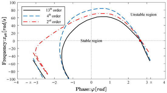
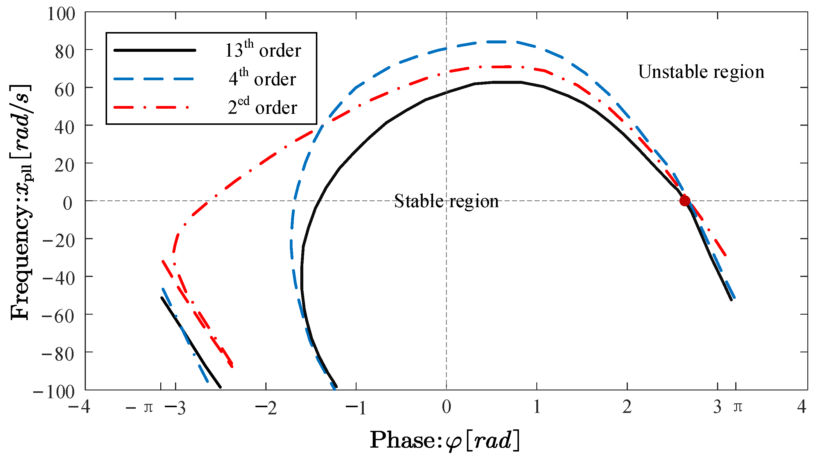
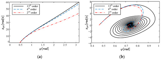
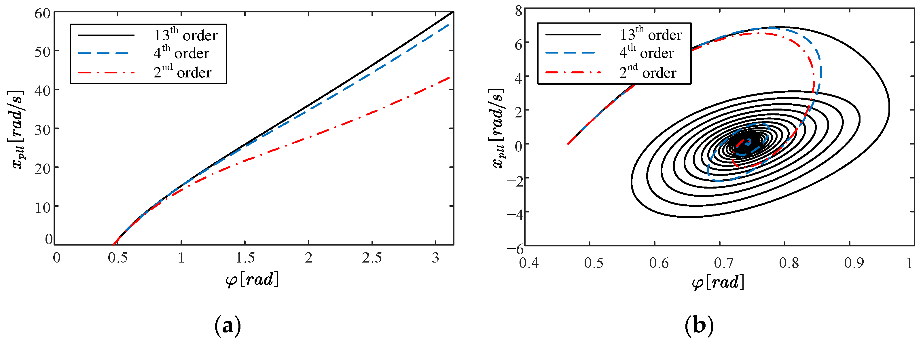
Firstly, the BOAs of GFL converter-based systems by different order models are compared. As shown in Figure 4, the black solid, blue dot dashed, and red dashed lines denote the boundaries of BOAs by 13th-, 4th-, and 2nd-order models on the φ-x_pll plane, respectively. The horizontal coordinate represents the periodic phase angle of the PLL, ranging from −π to π. The vertical coordinate represents the PLL output frequency. Crucially, the 4th-order model accurately approximates the full-order model’s stability boundary. Meanwhile, it can be seen that the differences between the boundaries of the full-order, 4th-order, and 2nd-order models are small in the first quadrant. It should be noted that the fault trajectory is generally located in the first quadrant, and thus the intersection between the fault trajectory and the BOA is generally located in the first quadrant. The BOA in the first quadrant can be seen as the most critical region.

Figure 4. BOAs of different order models for the GFL converter with voltage control.

Furthermore, for the hyperplane in the φ-x_pll plane, the tangent hyperplane based on the full-order model satisfies:

$$\begin{array}{l}0.6585\phi +0.0069x_{\mathrm{pll}}+0.2362x_{\mathrm{dvc}}+0.6686u_{\mathrm{dc}}+0.1736x_{\mathrm{tvc}}+0.1205x_{\mathrm{acc}1}\\ +0.0885x_{\mathrm{acc}2}+0.0037i_{\mathrm{d}}+0.0027i_{\mathrm{q}}+0.0049u_{\mathrm{td}}+0.0025u_{\mathrm{tq}}+0.0186i_{\mathrm{gd}}-0.1037i_{\mathrm{gq}}=0\end{array}$$

(21)

where the coefficients of the tangent hyperplane are calculated based on a group of typical parameters.

Meanwhile, the tangent hyperplane based on the 4th-order model satisfies:

$$0.6101\phi +0.0064x_{\mathrm{pll}}+0.2747x_{\mathrm{dvc}}+0.7432u_{\mathrm{dc}}=0$$

(22)

For the tangent hyperplane based on the 2nd-order model, it satisfies:

$$0.9999\phi +0.0147x_{\mathrm{pll}}=0$$

(23)

Combining Equation (22)–(24), for the coefficient of state variables φ and x_pll (marked by red), it can be seen that the 4th-order model can depict the full-order model well. In addition, it can be seen that the dominant parameters of the 4th-order model are similar to those of the full-order model.

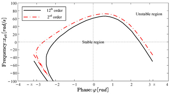
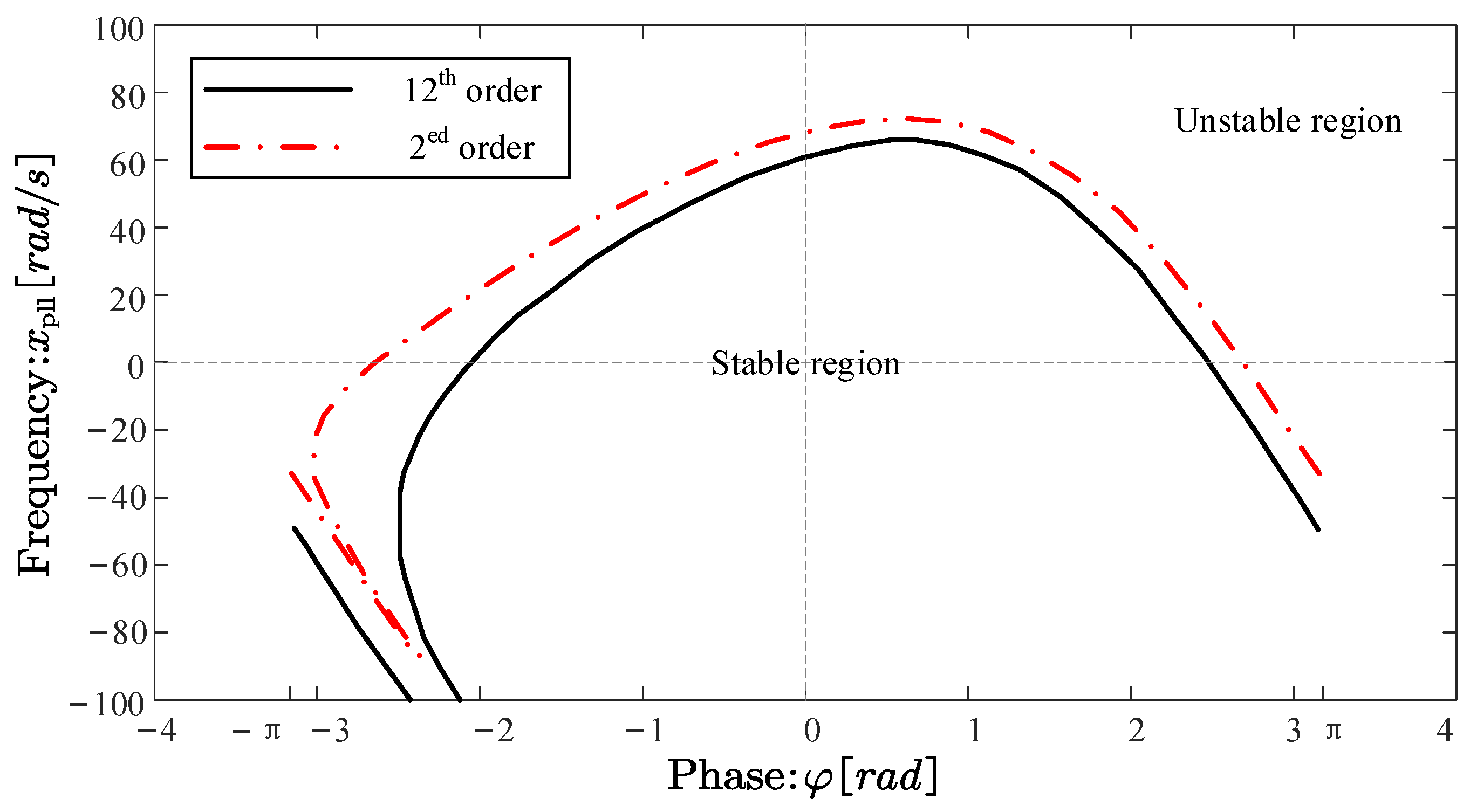
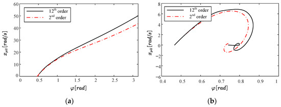
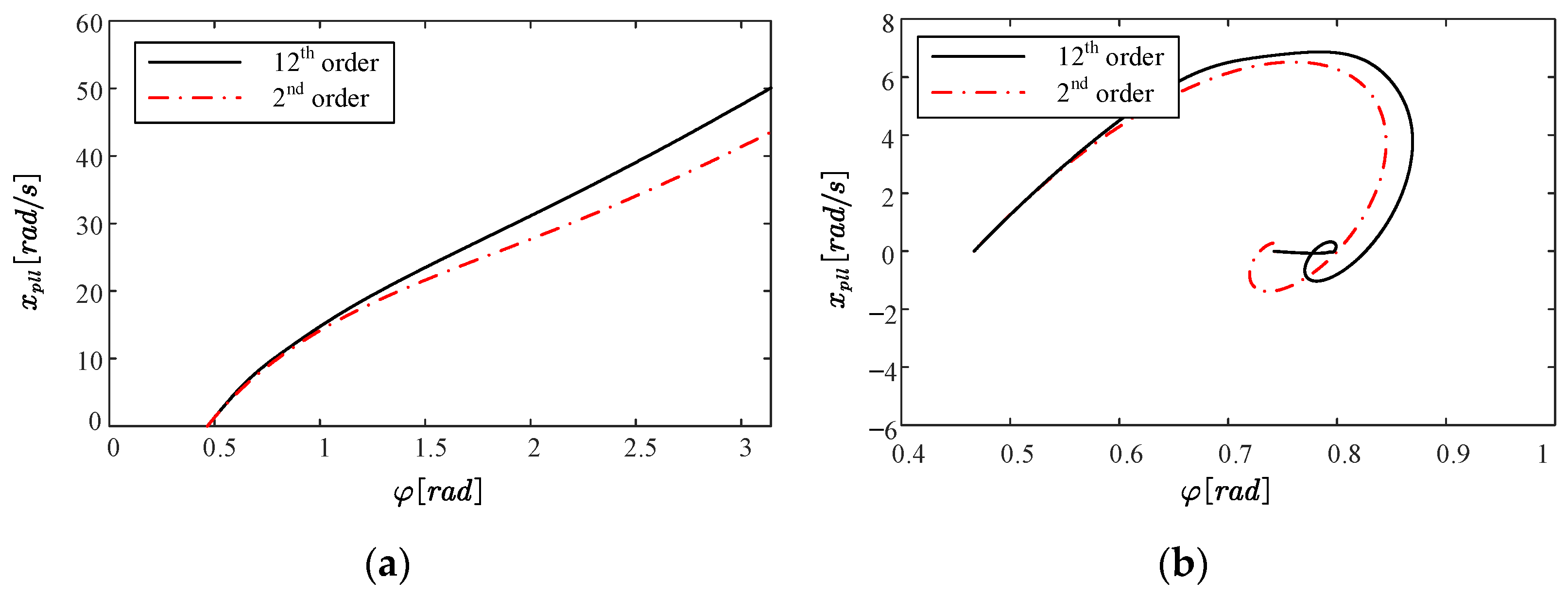
For the GFL converter-based systems with power control, the BOAs by different order models are compared in Figure 5, where the horizontal coordinate represents the phase angle of the PLL, and the vertical coordinate represents the PLL output frequency. In Figure 5, the black solid and red dashed lines separately denote the boundaries of BOAs by 12th- and 2nd-order models. It can be seen that the boundary of the 2nd-order model can depict that of the full-order model well in the first quadrant. Furthermore, for the hyperplane in the φ-x_pll plane, the tangent hyperplane based on the full-order model satisfies:

$$\begin{array}{l}0.1176x_{\mathrm{apc}}+0.5203x_{\mathrm{rpc}}+0.8390\phi +0.0117x_{\mathrm{pll}}+0.0444x_{\mathrm{acc}1}+0.0100x_{\mathrm{acc}2}\\ +0.0009i_{\mathrm{d}}+0.0002i_{\mathrm{q}}+0.0048u_{\mathrm{td}}+0.0010u_{\mathrm{tq}}+0.0011i_{\mathrm{gd}}-0.0967i_{\mathrm{gq}}=0\end{array}$$

(24)

Figure 5. BOAs of different order models for the GFL converter with power control.

For the hyperplane based on the 2nd-order model, it is the same as Equation (24).

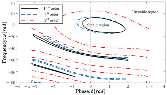
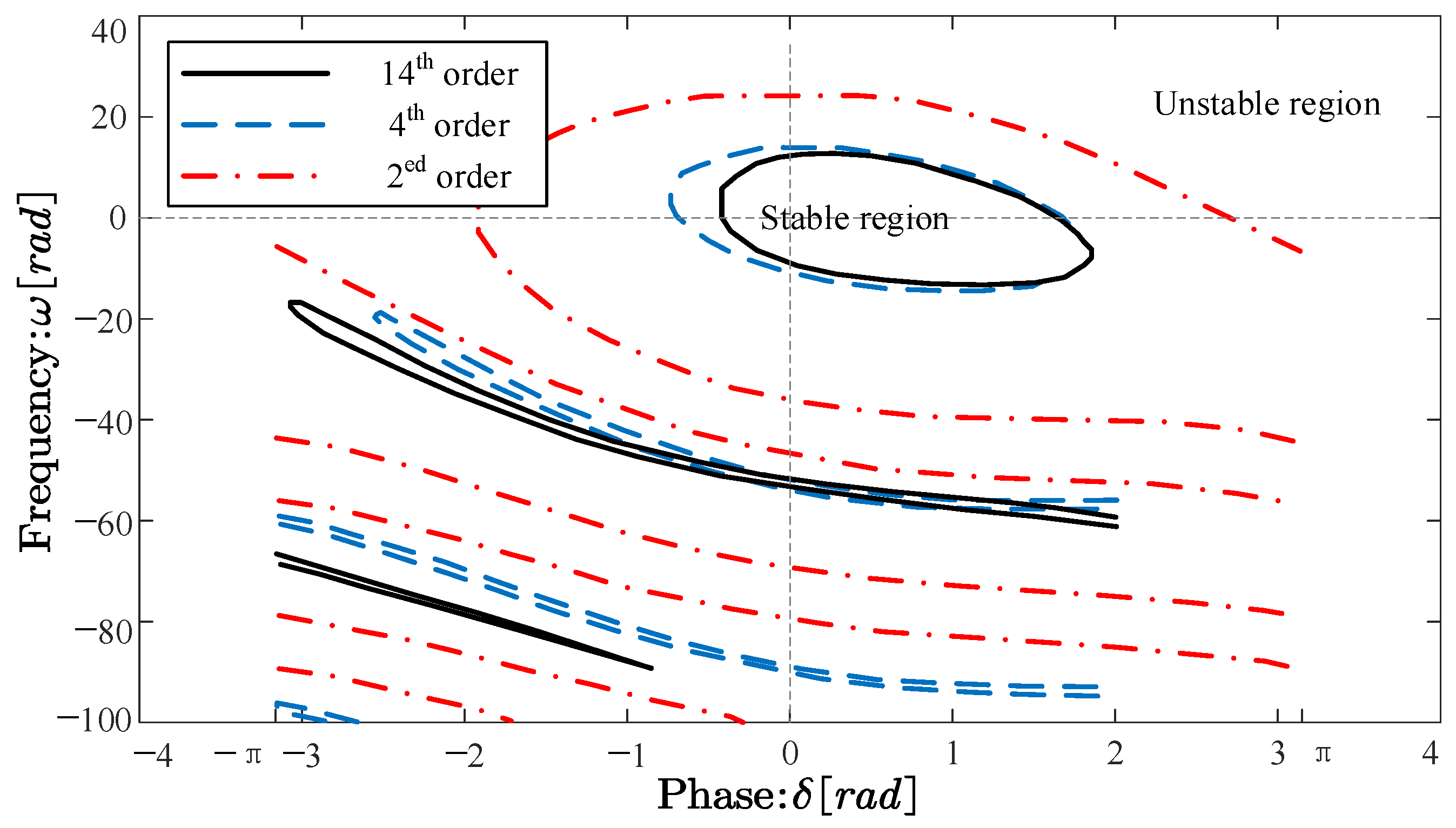
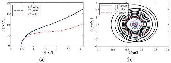
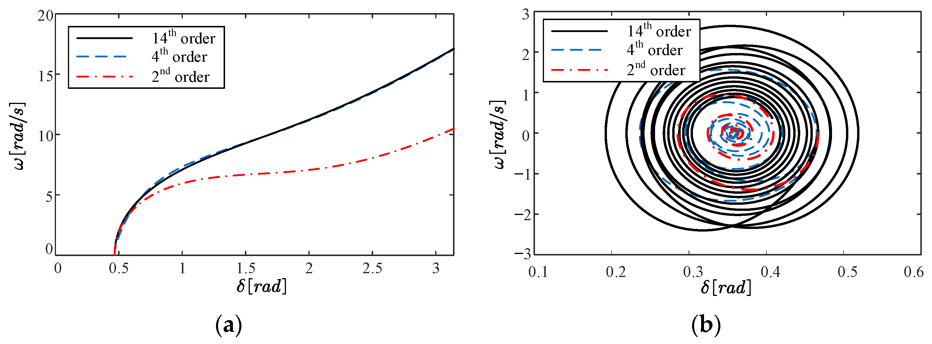
For the GFM converter-based systems, the boundaries of different regions are illustrated in Figure 6 in the δ-ω plane. The horizontal coordinate represents the phase angle of the VSG, which is periodic and ranges from −π to π. The vertical coordinate represents the VSG output frequency. As shown in Figure 6, the black solid, blue dot dashed, and red dashed lines denote the boundaries of BOAs by 14th-, 4th-, and 2nd-order models, respectively. Meanwhile, when state variables are within the BOA, the system can converge to the stable equilibrium point. On the contrary, the system can diverge when the state variables are outside the BOA. Crucially, differences between boundaries of the full order and 4th order are small, while the 2nd model has certain errors.

Figure 6. BOAs of different order models for the GFM converter with VSG or droop control.

For the tangent hyperplane in the δ-ω plane, it can be formulized as:

$$\begin{array}{l}0.9057\delta +0.0512\omega +0.3727x_{\mathrm{dvc}}+0.1559u_{\mathrm{dc}}-0.0317x_{\mathrm{tvc}1}+0.1116x_{\mathrm{tvc}2}-0.0006x_{\mathrm{acc}1}\\ +0.0022x_{\mathrm{acc}2}-0.000i_{\mathrm{d}}+0.000i_{\mathrm{q}}+0.0010u_{\mathrm{td}}+0.0002u_{\mathrm{tq}}+0.0040i_{\mathrm{gd}}-0.0202i_{\mathrm{gq}}=0\end{array}$$

(25)

Meanwhile, the tangent hyperplane by the 4th-order model equals:

$$0.9071\delta +0.0519\omega +0.3848x_{\mathrm{dvc}}+0.1626u_{\mathrm{dc}}=0$$

(26)

And, for the tangent hyperplane based on the 2nd-order model, it satisfies:

$$0.9979\delta +0.0643\omega =0$$

(27)

Thus, based on the coefficients of state variables δ and ω (marked by red), it can be seen that the 4th-order model can depict the full-order model well. In addition, it can be seen that the dominant parameters of the 4th-order model are similar to those of the full-order model.

3.3. Comparisons of Phase Trajectories Under Different Large-Signal Disturbances

In addition to the boundaries of BOAs, the fault trajectories are another determining factor for the justification of transient stability. By the phase trajectory method, the phase trajectories of the GFL VSC in the φ-ω_pll plane under different large-signal disturbances are depicted in Figure 7, where Figure 7a,b show separately the voltage dip and increase in grid impedance. As shown in Figure 7, for the GFL converter controlled by the voltage outer loop, the fourth-order equation can describe the dynamics in the transient process of the original higher-order equation well. Compared with the 4th-order equation, the 2nd-order equation has a slight error, but it can basically describe the transient dynamic process of the original equation.

Figure 7. Phase diagram curves of different order models for the GFL converter with voltage controls. (a) U_g dips to 0.30 p.u. (b) L_g increases to 0.75 p.u.

As shown in Figure 8, the phase diagram curves of different order models are separately depicted for the GFL converter with power controls, separately for the voltage dip and increase in the grid impedance.

Figure 8. Phase diagram curves of different order models for the GFL converter with power controls. (a) U_g dips to 0.30 p.u. (b) L_g increases to 0.75 p.u.

As shown in Figure 9, the phase diagram curves of different order models are separately depicted for the GFL converter with power controls, separately for the voltage dip and increase in the grid impedance. Among them, the phase trajectory of the 4th-order equation after the fault is almost exactly the same as that of the original equation, and the transient phase trajectory of the 2nd-order equation is also basically close to that of the original equation.

Figure 9. Phase diagram curves of different order models for the GFM converter with VSG or droop control. (a) U_g dips to 0.30 p.u. (b) L_g decreases to 0.20 p.u.

3.4. Comparison of Critical Clearing Times (CCTs)

The critical clearing time (CCT) and angle (CCA) are important criteria for quantifying the transient stability margin in power systems. The CCT can be estimated by determining the intersection point of the during-fault trajectory and the boundary of the BOA (Section 3.1). Thus, this section compares the errors between the CCT estimated by different models and the CCT obtained by electromagnetic transient (EMT) simulation, thereby proving the accuracy of the dominant link and the equation obtained. This type of disturbance only affects the system trajectory during the fault and has no impact on the stable domain of the system after the fault. Therefore, in this section, the infinite-bus voltage U_g drops from 1.0 p.u. to 0.7 p.u. and then returns to 1.0 p.u. as the test scenario for the simulation analysis. The CCT obtained through multiple tests of EMT simulation (dichotomy) is taken as its benchmark value. For the simulation-based method, the CCT is determined through iterative EMT simulations. In detail, multiple simulation tests are conducted to determine whether the system can remain stable after the chosen clearing time. After multiple simulation tests, the CCT can be narrowed within a certain range by the dichotomy.

For the GFL converter-based system under the voltage outer loop, the CCT obtained through EMT simulation is 0.0962 s. Based on the full-order model, the 4th-order model, and the 2nd-order model, the specific calculation results of the fault CCT obtained by linear and square estimation are shown in Table 4. It can be seen that the difference between the CCT estimated based on the 4th-order model (considering four state variables) and that estimated by the full-order model (considering all state quantities) is relatively small, and the increase in estimation error is not significant. Among them, the linear estimation shows that the difference between the two is only 0.0019 s (1.98%), and the quadratic estimation shows that the difference between the two is 0.0045 s (4.68%). For the 2nd-order equation, that is, only considering the two state variables of the PLL control link (i.e., φ and x_pll), the error between the estimated CCT and the CCT obtained based on the full-order model is relatively small. Among them, the linear estimation shows that the difference between the two is 0.0092 s, and the quadratic estimation shows that the difference between the two is 0.0023 s. Compared with the 4th-order model, the estimation error of the 2nd-order model has increased. As the boundaries of BOAs are estimated by linear and quadratic hypersurfaces, estimated CCTs still have errors when the full-order model is applied. When the EAC method based on the 2nd-order model is applied, the estimated CCT is 0.0835 s with 13.20% relative errors (conservative).

Table 4. Comparison of CCTs calculated by different order models of GFL converter with voltage controls.

Model Order	Linear [s]	Error [%]	Quadratic [s]	Error [%]
Full order	0.1051	9.25	0.1011	5.09
Forth order	0.1070	11.23	0.1056	9.77
Second order	0.1143	18.81	0.1034	7.48

Consequently, it can be considered that the 4th-order model demonstrates structural fidelity in capturing the transient stability boundary of the original system, while the 2nd-order model offers computational simplicity.

For the GFL VSC under the power outer loop, the CCT obtained through EMT simulation is 0.3897 s. Based on the full-order model and the 2nd-order model, the specific calculation results of the fault CCT obtained by using linear estimation and quadratic estimation are shown in Table 5. It can be seen that the error of estimating CCT based on the 2nd-order equation is less than 5%. Meanwhile, for linear estimation, the difference between the CCT obtained based on the full-order equation and the 2nd-order equation is 0.0162 s. For the quadratic estimation, the difference between the two is 0.0244 s. In conclusion, it can be considered that the 2nd-order equation can well-describe the boundary of the transient stability domain of the GFL converter-based system under the control of the power outer loop.

Table 5. Comparison of CCTs calculated by different order models of GFL converter with power controls.

Model Order	Linear [s]	Error [%]	Quadratic [s]	Error [%]
Full order	0.3900	0.08	0.4207	7.95
Second order	0.4062	4.23	0.3963	1.69

For the GFM converter-based system, the CCT obtained through EMT simulation is 1.0986 s. Based on the full-order model, the 4th-order model, and the 2nd-order model, the specific calculation results of the fault CCT obtained by linear and quadratic estimation are shown in Table 6. Among them, the difference between the CCT estimated based on the 4th-order model (considering four state variables) and that estimated by the full-order model (considering all state variables) is relatively small, and the increase in estimation error is not significant. The difference between the linear estimates of the two is only 0.0167 s (1.52%), and the difference between the quadratic estimates is 0.0105 s (0.96%). For the 2nd-order equation, namely, only considering the two state variables of the PLL control link (i.e., δ and ω), the difference between the estimated CCT obtained and the CCT obtained based on the full-order model is relatively small. Among them, the difference between the linear estimations of the two is 0.0595 s (5.42%), and the difference between the quadratic estimations is 0.0514 s (4.68%). Compared with the 4th-order model, the error of the CCT obtained by the 2nd-order equation has increased. Therefore, the 4th-order equation can describe the boundary of the transient stability domain of the original system quite well. Although the error of the 2nd-order equation is slightly larger, it can basically reflect the boundary of the stable domain of the higher-order system.

Table 6. Comparison of CCTs calculated by different order models of GFM converter.

Model Order	Linear [s]	Error [%]	Quadratic [s]	Error [%]
Full order	1.1818	7.57	1.1756	7.01
Forth order	1.1985	9.09	1.1651	6.05
Second order	1.2413	12.99	1.2270	11.69

In conclusion, the 4th-order model achieves 95% boundary fidelity in characterizing BOAs of original converter systems. By combining results of BOA geometry, large-signal trajectory sensitivity, and CCT validation, the 4th-order model proves essential for precise DSR approximation, both for GFL and GFM converter-based systems. Meanwhile, for computation burden, employing reduced-order models to determine intersections between fault trajectories and the BOA alleviates computational overhead. Specifically, the computational efficiency has significantly improved for multi-converter systems by reduced-order models, which can be further studied in the future.

4. Definition and Approximation of Generalized Dynamic Security Region of Converter-Based Systems

The dynamic security region (DSR) of the power system is a powerful tool for power grid planning and online operation in engineering practice. It has been well-developed and applied worldwide. DSR is of great significance for dispatchers to prevent the development and expansion of transient accidents. For SG-dominated systems, due to local reactive power compensation, DSR is traditionally defined within the active power injection space of adjustable SGs, representing the set of active power values ensuring transient stability under given fault scenarios. However, with renewable generation displacing SGs as the primary power source, the definition of DSR should be enriched and redefined.

Transient synchronization stability refers to the ability of the grid to maintain synchronism following voltage dips or short-circuit faults. Meanwhile, if the system can maintain transient stability after a given fault (e.g., short-circuit faults are cleared by the relay after 0.1 s), it is said that the operating state (active power injections) is dynamically secure. In SG-dominated systems, DSR is a set composed of SG’s active powers, and is formally defined as:

$${\Omega }_{DSR}=\{u:\varphi (u)\in B(x_{\mathrm{s}}(u))\}$$

(28)

where u is the active power injections of the SG. ϕ(u) represents the state variables at the moment of fault clearance. B(x_s(u)) represents the BOA of the stable equilibrium point x_s.

4.1. Type 1 Dynamic Security Region

Borrowed from the SG-dominated system, Type 1 DSR is also defined in the space of active power injections, i.e., the d-axis active current reference $i_{\mathrm{d}}^{\mathrm{ref}}$ of the converter. Therefore, Type 1 DSR of the converter-based system can be formalized as:

$${\Omega }_{\mathrm{DSR}}=\{i_{\mathrm{d}}^{\mathrm{ref}}:\varphi (i_{\mathrm{dref}})\in B(x_{\mathrm{s}}(i_{\mathrm{d}}^{\mathrm{ref}}))\}$$

(29)

where ϕ(u) represents the state variables at the moment of fault clearance. B(x_s(u)) represents the BOA of the stable equilibrium point x_s. In this respect, for the power system composed of SGs and converters, Type 1 DSR should be constituted by the reference values of the active power of the SG and the active current of the converter.

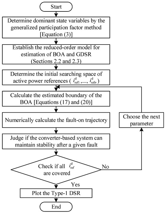
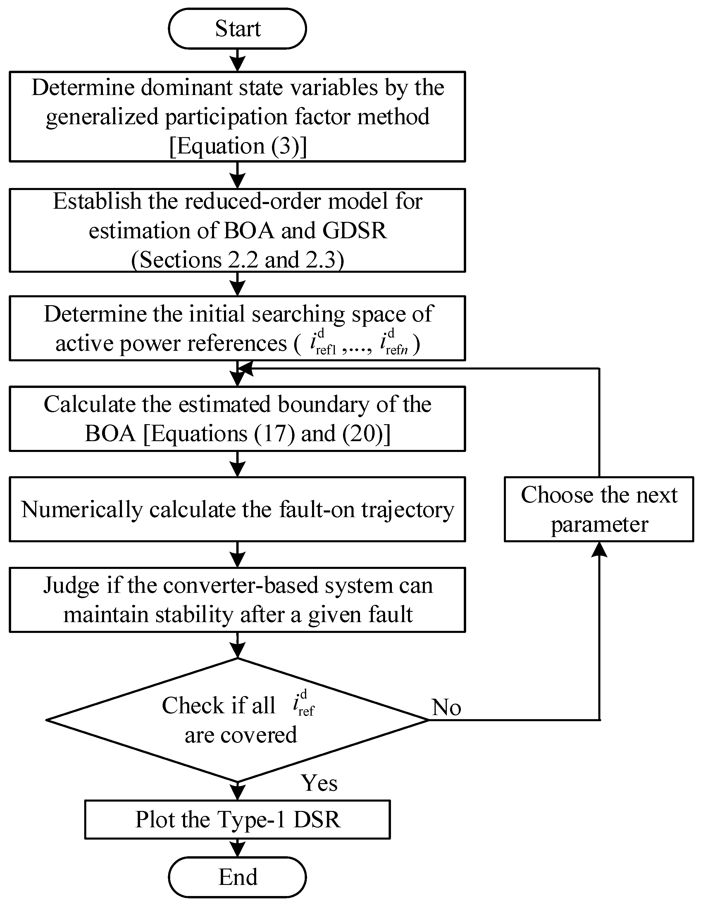
In detail, the procedure of Type 1 DSR estimation consists of six steps, as shown in Figure 10. Firstly, the dominant state variables of the converter-based system should be determined by the proposed GPF method, as shown in Equation (3) in Section 2. Secondly, according to the determined state variables, the reduced-order model can be established, as shown in Section 2.2 and Section 2.3, where typical GFL and GFM converters are studied. The dominant state variables and reduced-order models of converters with novel controls can be similarly analyzed following the proposed method in Section 2. Thirdly, an initial searching parameter space of Type 1 DSR is determined according to its normal value, where the searching space is composed of the active current reference values $i_{\mathrm{d}}^{\mathrm{ref}}$ of converters. Fourthly, the boundary of BOA under the given $i_{\mathrm{d}}^{\mathrm{ref}}$ is estimated by the manifold method, as shown in Equations (17) and (20), and Section 3. Following this, the fault-on trajectory of converter-based systems is numerically calculated further for stability determination. Finally, judge if the converter-based systems can maintain stability after a given fault. After examining all $i_{\mathrm{d}}^{\mathrm{ref}}$ in the initial searching space, Type 1 DSR can be illustrated in the space of active power injections.

Figure 10. The procedure of the proposed Type 1 DSR approximation method.

For the GFL converter-based system, there exists a maximum d-axis current reference value $i_{\mathrm{dref}}^{\max }$, which enables the system to maintain transient stability under the given fault. Generally, the fault can be cleared by the relay after 4–5 cycles (0.08–0.1 s for 50 Hz) in engineering practice. In this respect, when U_g dips to 0.70 p.u., the maximum $i_{\mathrm{dref}}^{\max }$ is shown in Table 7 based on the EMT simulation method and the quadratic approximation. As shown in the third row of Table 7, the maximum $i_{\mathrm{dref}}^{\max }$ obtained based on the quadratic approximation is 0.98 p.u., when U_g dips to 0.7 p.u. and recovers to 1.0 p.u. after 0.1 s. Meanwhile, the EMT simulation result is 0.89 p.u., with an absolute error of 0.09 and a relative error of 10.11%. Therefore, the quadratic approximation can provide a relatively accurate DSR estimate for a single VSC system.

Table 7. Estimated $i_{\mathrm{dref}}^{\max }$ under different clearing times for the GFL converter-based system with voltage controls.

Clearing Time [s]	EMT [p.u.]	Quadratic [p.u.]	Absolute Error [s]	Relative Error [%]
0.08 (4 cycle)	0.95	1.03	0.08	8.42%
0.10 (5 cycle)	0.89	0.98	0.09	10.11%
0.12 (6 cycle)	0.85	0.93	0.08	9.41%

For the GFL converter-based system with power control, the maximum $i_{\mathrm{dref}}^{\max }$ is shown in Table 8 based on the EMT simulation method and the quadratic approximation when U_g dips to 0.55 p.u. and recovers to 1.0 p.u. after 0.1 s. As shown in the third row of Table 8, the maximum $i_{\mathrm{dref}}^{\max }$ obtained based on the quadratic approximation is 0.97 p.u., while the EMT simulation result is 0.89 p.u., with an absolute error of 0.08 s and a relative error of 8.99%.

Table 8. Estimated $i_{\mathrm{dref}}^{\max }$ under different clearing times for the GFL converter-based system with power controls.

Clearing Time [s]	EMT [p.u.]	Quadratic [p.u.]	Absolute Error [s]	Relative Error [%]
0.08 (4 cycle)	0.96	1.03	0.07	7.29%
0.10 (5 cycle)	0.89	0.97	0.08	8.99%
0.12 (6 cycle)	0.84	0.90	0.06	7.14%

For the GFM converter-based system with power control, the maximum $i_{\mathrm{dref}}^{\max }$ is shown in Table 9 based on the EMT simulation method and the quadratic approximation when U_g dips to 0.10 p.u. and recovers to 1.0 p.u. after 0.1 s. As shown in the third row in Table 9, the maximum $i_{\mathrm{dref}}^{\max }$ obtained based on the quadratic approximation is 0.92 p.u. while the EMT simulation result is 0.85 p.u., with an absolute error of 0.07 s and a relative error of 8.24%.

Table 9. Estimated i_dref under different clearing times for the GFM converter-based system.

Clearing Time [s]	EMT [p.u.]	Quadratic [p.u.]	Absolute Error [s]	Relative Error [%]
0.08 (4 cycle)	0.91	0.98	0.07	7.70%
0.10 (5 cycle)	0.85	0.92	0.07	8.24%
0.12 (6 cycle)	0.80	0.86	0.06	7.50%

4.2. Type 2 Dynamic Security Region (Generalized Dynamic Security Region)

As the SG can only regulate its active power to improve the stability margin of the system, the classical DSR is defined in the space of active power injection. Converter-dominated systems exhibit multidimensional controllability through power setpoints and control parameters. Inspired by this, according to the controllable parameters, Type 2 DSR (GDSR) is defined in the space of controllable parameters, namely, as follows:

$${\Omega }_{\mathrm{DSR}}=\{k_{\mathrm{controlled}}:\varphi (i_{\mathrm{dref}})\in B(x_{\mathrm{s}}(k_{\mathrm{controlled}}))\}$$

(30)

where k_controlled can be chosen as k_ppll, k_ipll, M, D, etc. Thus, for the power system composed of the SG and converter or 100% converter-based systems, there exists Type 2 DSR, which consists of controllable parameters. What is more, existing parameter-space stability regions address small-signal stability and wideband oscillations, whereas the proposed Type 2 DSR targets large-signal (transient) synchronization. In other words, the controllable parameters can affect the trainset stability of the converter-based system. On the one hand, the system can maintain transient stability after a given fault when the controllable parameters are within the DSR. On the other hand, the system can be adjusted for transient stability by changing the controllable parameters.

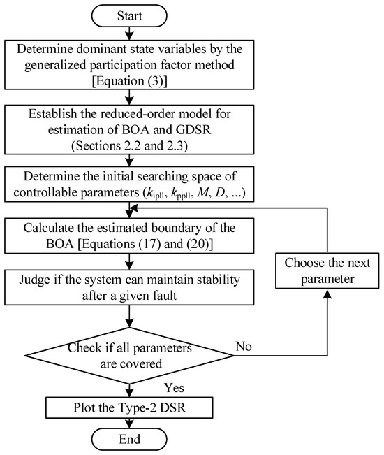
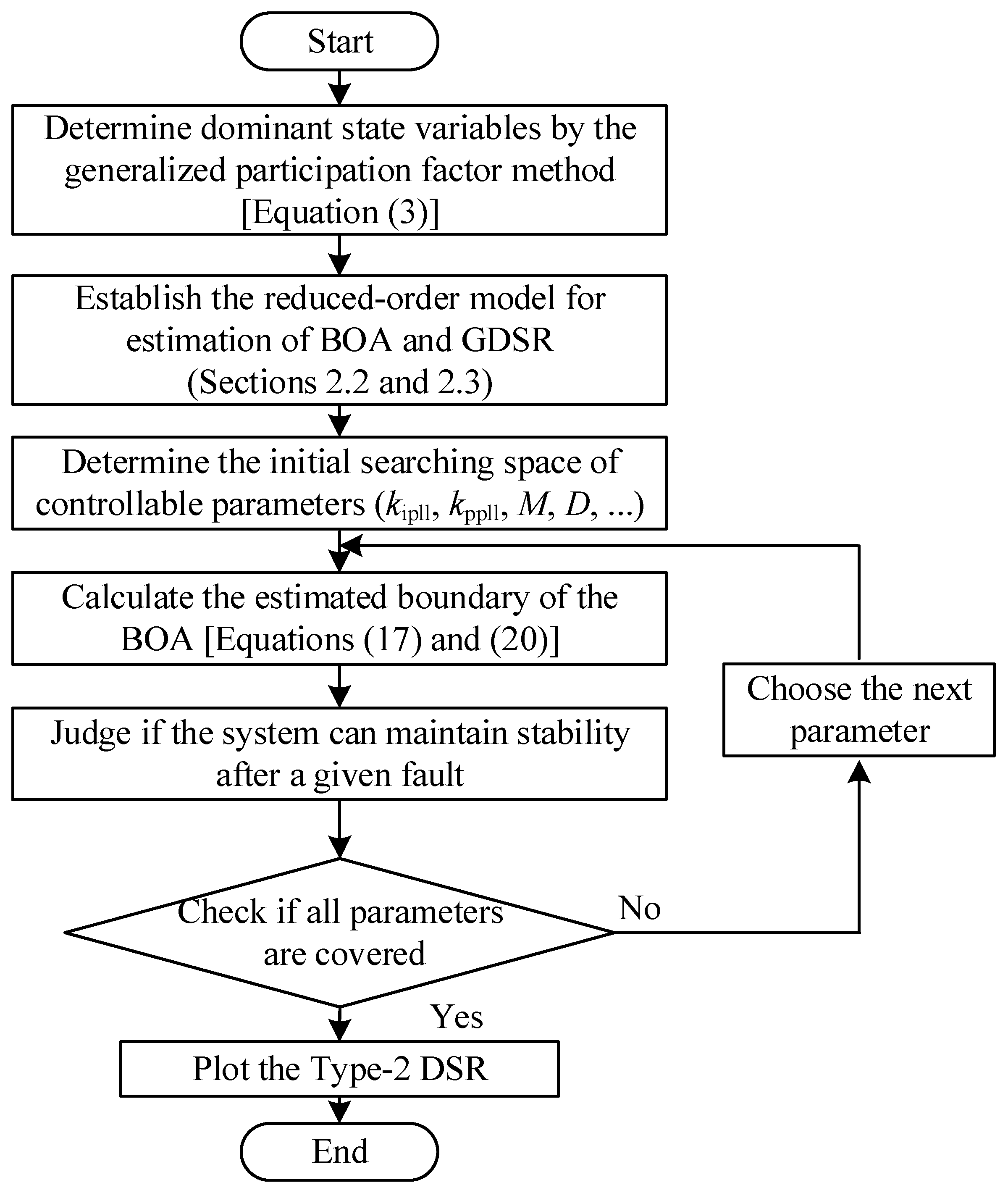
The estimation of Type 2 DSR comprises five sequential steps analogous to the methodology in Section 4.1. As illustrated in Figure 11, the procedure of Type 2 DSR estimation consists of six steps, which similarly initiate the identification of dominant state variables of the converter-based system. Secondly, a reduced-order model is constructed based on the identified state variables, as shown in Section 2. Thirdly, the initial search parameter space, encompassing controllable parameters of dominant control loops (e.g., k_ppll, k_ipll, M, D, etc.), is then defined. Fourthly, the boundary of BOA is estimated under specified parameter sets using the method of manifold [Equations (17) and (20)]. Fifthly, judge whether the converter-based systems can maintain transient synchronous stability after a given fault. After examining all the parameters, Type 2 DSR can be delineated within the controllable domain.

Figure 11. The procedure of the proposed Type 2 (GDSR) approximation method.

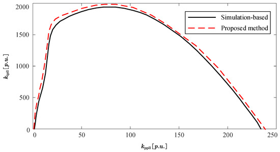
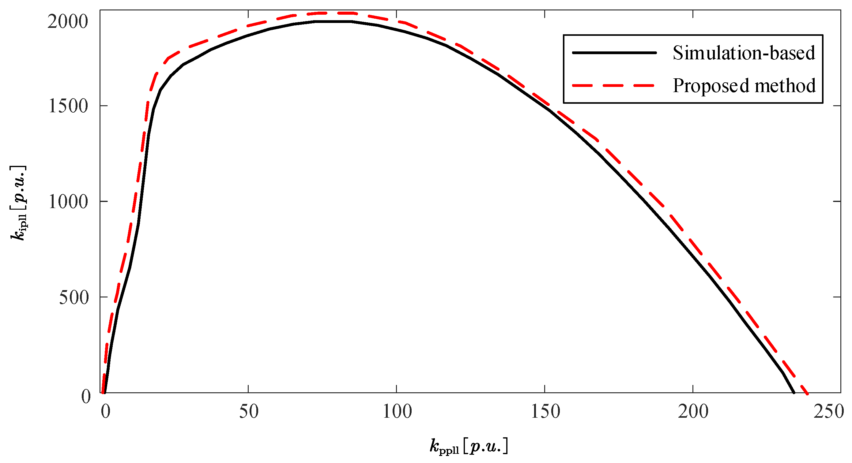
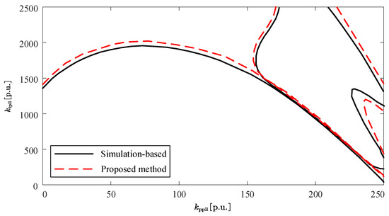
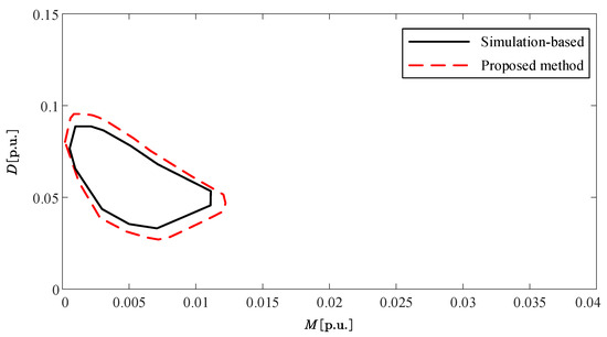
To validate the accuracy and effectiveness of the proposed method for estimating the GDSR, results are compared with the proposed method and the EMT simulation method, as shown in Figure 12, Figure 13 and Figure 14. Crucially, the converter-based system maintains transient stability under given faults if and only if its parameter set resides within Type 2 DSR. As shown in Figure 12, DSRs determined by the simulation-based approach and proposed method are separately denoted by black solid and red dashed lines, where the horizontal coordinate represents the PLL’s proportional gain k_ppll, and the vertical coordinate represents the PLL’s integral gain k_ipll. Both PI gains of the PLL are in per-unit values (p.u.). In detail, the convert-based system can maintain stability after the given fault when the parameter set (k_ppll and k_ipll) is within Type 2 DSR, where the given fault is such that the grid voltage dips to 0.70 p.u. and recovers after 0.10 s (five cycles). It can be seen that there is consistency between boundaries in simulation-based and proposed approaches. The mean relative error is smaller than 10% with optimistic estimation.

Figure 12. Comparison of DSRs by the simulation-based (solid line) and proposed method (dashed line) for the GFL converter with voltage control.

Figure 13. Comparison of DSRs in the simulation-based (solid line) and proposed methods (dashed line) for the GFL converter with power control.

Figure 14. Comparison of DSRs by the simulation-based and proposed method for the GFM converter.

Figure 13 quantitatively compares DSRs derived from simulation-based approaches (black solid lines) and the proposed method (red dashed lines) for the GFL converter-based system conducted under power control configuration, where the horizontal coordinate represents the PLL’s proportional gain k_ppll, and the vertical coordinate represents the PLL’s integral gain k_ipll. For physical interpretation, the convert-based system can maintain stability after the given fault when the parameter set (k_ppll and k_ipll) is within Type 2 DSR, where the given fault is that the grid voltage dips to 0.55 p.u. and recovers after 0.10 s (five cycles). Meanwhile, it can be seen that there is consistency between boundaries in these two approaches, while the proposed method gives optimistic estimations.

Figure 14 compares DSR for the GFM converter-based system via the simulation-based (black solid lines) and proposed method (red dashed lines). In Figure 14, the horizontal coordinate represents the VSG’s inertia M, and the vertical coordinate represents the VSG’s damping D. Both the inertia and damping are in per-unit values (p.u.). For the physical interpretation, the convert-based system can maintain stability after the given fault when the parameter set (M and D) is within Type 2 DSR, where the given fault is that the grid voltage dips to 0.10 p.u. and recovers after 0.10 s (five cycles). Similarly, there exists a small difference between boundaries in the two approaches.

In power system operations, the DSR provides two critical functions for system operators. Firstly, as the power grid is constantly confronted with various disturbances and faults, the operating state undergoes continuous changes. Thus, power grid operators can determine whether the current operating state of the power grid is secure and whether the power grid has a sufficient stability margin based on the pre-calculated DSR. Secondly, when stability margins degrade below safety thresholds, the DSR can guide grid operators to adjust the active power of generators and controllable parameters to enhance the security margin. For instance, operators can adjust the current operating state (including power injections and controllers’ parameters) to the geometric center of the DSR.

For Type 1 DSR, the estimated maximum $i_{\mathrm{dref}}^{\max }$ can be set as the limitation of the active power injection of the renewable generation. For application, when setting the operating condition of the power system, including the economic operation and dispatching control of the power system, etc., the Type 1 DSR provides the operating boundary for active injection. For Type 2 DSR, the stability margin can be improved by adjusting the controllable parameters. Taking Figure 12 as an example, the stability margin is small with the parameter set (k_ppll =50, k_ipll = 2000), which is critically unstable. It consists of the results in Table 7. In this respect, the system has sufficient stability margin with the parameter set (k_ppll =100, k_ipll = 1000), which is located at the geometric center of the DSR. As for Figure 13, the parameter set (k_ppll =100, k_ipll = 1000) is roughly located at the geometric center of the Type 2 DSR. As for Figure 14, the parameter set (M = 0.005, D = 0.06) is roughly located at the geometric center of the Type 2 DSR.

5. Discussion

The classic DSR is defined in the space of active power injections, while renewable-rich power systems necessitate expanded security paradigms that accommodate the higher-dimensional controllability of converter-based resources, including PI gains of dominant control loops (PLL and VSG). It is worthwhile have the following discussions.

Firstly, the proposed framework comprehensively analyzes the existing typical control strategies, including the GFL converter within power and voltage controls, and the GFM converter within the VSG and droop control. As the proposed approach is based on the general nonlinear systems and manifold theory, the methodology remains extensible to emerging strategies. Several novel control strategies can be studied in the future, such as virtual oscillator control or hybrid architectures.

Secondly, Type 1 and 2 DSRs of converter-based systems are estimated via BOA analysis using the manifold method. As the proposed approaches are based on the general differential equation and nonlinear dynamics, the approach applies beyond single-converter infinite-bus systems. For the heterogeneous multi-converter multi-bus system, the proposed approaches are still effective, while two key issues should be addressed. One is the determination of the CUPE. For a single-converter system, the only unstable equilibrium point is just the CUEP, while there exist multiple unstable equilibrium points for networked multi-converter systems. The CUEP of the multi-converter system can be determined by combining the fault trajectory and BOA, which is more complex than the single-converter system. The other one is the estimation of the BOA. For the BOA estimation of the multi-converter system, a more novel method can be adopted to estimate boundaries of the BOA and DSR to reduce the error, such as an AI-driven method, machine learning, etc.

Thirdly, unlike conventional model-order reduction techniques (e.g., the singular perturbation theory), the proposed method eliminates reliance on timescale separation. The timescale separation in the SG is natural, including sub-transient, transient, and synchronous states. By the singular perturbation theory, reduced-order models of the SG can be established. On the contrary, the timescales of various control loops depend on PI gains, which leads to deep couplings between different controls. The separation of timescale is not valid for renewable-rich systems.

Fourthly, the developed DSR framework provides grid operators with a powerful stability assessment tool. It enables operators to comprehensively evaluate the current operating state of the power system. By characterizing Type 1 and 2 DSR boundaries, operators can gain a clear understanding of the stability margin and the potential risks associated with the current operation condition. However, at present, the article does not provide specific methods on how to control and adjust the grid based on the proposed DSR. In light of the proposed DSRs, it is highly advisable to conduct further research on control strategies. These strategies should focus on adjusting controllable parameters. Additionally, they should also involve the adjustment of active power references. By precisely tuning these factors, it is expected to enhance the stability of the power grid, reduce the probability of instability events, and improve the overall performance and reliability of the grid operation. Further studies on control strategies can bridge the gap between the theoretical DSRs and engineering practice.

6. Conclusions

In summary, the article establishes a novel DSR framework for converter-based systems, advancing both methodological and conceptual foundations. Methodologically, two novel approaches are proposed for DSR approximation. For modeling, the generalized participation factor method is proposed for identifying dominant state variables and establishing reduced-order models in Section 2. For estimating boundaries, the linear and quadratic hypersurfaces are proposed to estimate the boundary of BOA by the manifold method. Conceptually, two kinds of DSR typologies are established by extending paradigms of SG-dominated power systems. Type 1 DSR reconceptualizes active power injection space as the active-current reference space of converters. Type 2 DSR is newly defined and encapsulates stability limits within the controllable parameter space of dominant control loops (e.g., PLLs, VSG). Together, these two kinds of DSRs extend the controllable dimensions of the renewable-rich system and provide grid operators with a quantitative tool to optimize converter control parameters when ensuring transient stability. Meanwhile, GFL and GFM converters are both analyzed by the proposed framework to validate their effectiveness.

References

- Tse, C.K.; Huang, M.; Zhang, X.; Liu, D.; Li, X.L. Circuits and Systems Issues in Power Electronics Penetrated Power Grid. IEEE Open J. Circuits Syst. 2020, 1, 140–156. [Google Scholar] [CrossRef] [Scilit]
- Li, X.; Zheng, J.; Liu, Y.; Zhou, X.; Yu, H.; Zhu, J.; Guo, L.; Wang, C. Small-Signal Synchronous Stability Analysis for 100% Power Electronics-Based Power System with Distributed Grid-Forming Converters. J. Mod. Power Syst. Clean Energy 2025. early access. [Google Scholar]
- Zhan, X.; Li, J.; Li, Z.; Gan, D. Parametric transient stability analysis using renormalization group approach. Int. J. Electr. Power Energy Syst. 2025, 172, 111326. [Google Scholar] [CrossRef] [Scilit]
- Kabalan, M.; Singh, P.; Niebur, D. Large Signal Lyapunov-Based Stability Studies in Microgrids: A Review. IEEE Trans. Smart Grid 2017, 8, 2287–2295. [Google Scholar] [CrossRef] [Scilit]
- Hu, J.; Guo, Z.; Zhu, J.; Kurths, J.; Hou, Y.; Du, B.; Wu, Z.; Zhao, G.; Liu, Y.; Xin, K.; et al. Electromagnetic Dynamic Stability Analysis of Power Electronics-Dominated Systems Using Eigenstructure-Preserved LTP Theory. Nat. Commun. 2025, 16, 6852. [Google Scholar] [CrossRef] [Scilit]
- Sajadi, A.; Kenyon, R.; Hodge, B. Synchronization in Electric Power Networks with Inherent Heterogeneity Up to 100% Inverter-Based Renewable Generation. Nat. Commun. 2022, 13, 2490. [Google Scholar] [CrossRef] [Scilit]
- Wang, X.; Taul, M.G.; Wu, H.; Liao, Y.; Blaabjerg, F.; Harnefors, L. Grid-synchronization stability of converter-based resources-An overview. IEEE Open J. Ind. Appl. 2020, 1, 115–134. [Google Scholar] [CrossRef] [Scilit]
- Kundur, P. Power System Stability and Control; McGraw-Hill: Columbus, OH, USA, 1994. [Google Scholar]
- Hu, Q.; Fu, L.; Ma, F.; Ji, F. Large Signal Synchronizing Instability of PLL-Based VSC Connected to Weak AC Grid. IEEE Trans. Power Syst. 2019, 34, 3220–3229. [Google Scholar] [CrossRef] [Scilit]
- Ma, R.; Zhang, Y.; Zhan, M.; Cao, K.; Liu, D.; Jiang, K.; Cheng, S. Dominant Transient Equations of Grid-Following and Grid-Forming Converters by Controlling-Unstable-Equilibrium-Point-Based Participation Factor Analysis. IEEE Trans. Power Syst. 2024, 39, 4818–4834. [Google Scholar] [CrossRef] [Scilit]
- Xu, H.; Zhan, M. Transient Synchronization Stability Analysis and Assessment of DFIG System Under Severe Faults. IEEE Trans. Power Electron. 2026, 41, 3894–3911. [Google Scholar] [CrossRef] [Scilit]
- Guo, J.; Zhai, D.; Li, X.; Wang, Z. Nonlinear Modeling and Transient Stability Analysis of Grid-Connected Voltage Source Converters during Asymmetric Faults Considering Multiple Control Loop Coupling. Appl. Sci. 2024, 14, 7834. [Google Scholar] [CrossRef] [Scilit]
- Fu, X.; Sun, J.; Huang, M.; Tian, Z.; Yan, H.; Iu, H.H.-C.; Hu, P.; Zha, X. Large-Signal Stability of Grid-Forming and Grid-Following Controls in Voltage Source Converter: A Comparative Study. IEEE Trans. Power Electron. 2021, 36, 7832–7840. [Google Scholar] [CrossRef] [Scilit]
- Ma, R.; Li, J.; Kurths, J.; Cheng, S.; Zhan, M. Generalized Swing Equation and Transient Synchronous Stability with PLL-Based VSC. IEEE Trans. Energy Convers. 2022, 37, 1428–1441. [Google Scholar] [CrossRef] [Scilit]
- He, X.; Duarte, J.; Häberle, V.; Dörfler, F. Aggregate Grid-Forming Control of Distributed Energy Resources. IEEE Trans. Smart Grid 2026. early access. [Google Scholar]
- Yang, J.; Tse, C.K.; Huang, M.; Fu, X. Homoclinic bifurcation of a grid-forming voltage source converter. IEEE Trans. Power Electron. 2021, 36, 13176–13187. [Google Scholar] [CrossRef] [Scilit]
- Qu, Q.; Xiang, X.; Xin, K.; Liu, Y.; Li, W.; He, X. Transient Stability Analysis of Hybrid GFL-GFM System Considering Various Damping Effects. IEEE Trans. Ind. Electron. 2025, 72, 13334–13347. [Google Scholar] [CrossRef] [Scilit]
- Luo, C.; Ma, X.; Liu, T.; Wang, X. Controller-saturation-based transient stability enhancement for grid-forming inverters. IEEE Trans. Power Electron. 2023, 38, 2646–2657. [Google Scholar] [CrossRef] [Scilit]
- Li, Y.; Gu, Y.; Green, T.C. Revisiting grid-forming and grid-following inverters: A duality theory. IEEE Trans. Power Syst. 2022, 37, 4541–4554. [Google Scholar] [CrossRef] [Scilit]
- Kaye, R.; Wu, F. Dynamic security regions of power systems. IEEE Trans. Circuits Syst. 1982, 29, 612–623. [Google Scholar] [CrossRef]
- Xue, A.; Wu, F.F.; Lu, Q.; Mei, S. Power system dynamic security region and its approximations. IEEE Trans. Circuits Syst. I Regul. Pap. 2006, 53, 2849–2859. [Google Scholar] [CrossRef] [Scilit]
- Yu, Y.; Liu, Y.; Qin, C.; Yang, T. Theory and Method of Power System Integrated Security Region Irrelevant to Operation States: An Introduction. Engineering 2020, 6, 754–777. [Google Scholar] [CrossRef] [Scilit]
- Ma, R.; Zhan, M. Transient Stability Assessment and Dynamic Security Region in Power Electronics Dominated Power Systems. In Proceedings of the 2022 IEEE International Conference on Power Systems Technology (POWERCON), Kuala Lumpur, Malaysia, 12–14 September 2022; IEEE: New York, NY, USA, 2022; pp. 1–6. [Google Scholar]
- Ren, J.; Zeng, Y.; Qin, C. Practical Dynamic Security Region Model: A Hybrid Physical Model-Driven and Data-Driven Approach. IEEE Trans. Power Syst. 2025, 40, 728–739. [Google Scholar] [CrossRef] [Scilit]
- Yee, H.; Spalding, B.D. Transient Stability Analysis of Multimachine Power Systems by the Method of Hyperplanes. IEEE Trans. Power Appar. Syst. 1977, 96, 276–284. [Google Scholar] [CrossRef] [Scilit]
Disclaimer/Publisher’s Note: The statements, opinions and data contained in all publications are solely those of the individual author(s) and contributor(s) and not of MDPI and/or the editor(s). MDPI and/or the editor(s) disclaim responsibility for any injury to people or property resulting from any ideas, methods, instructions or products referred to in the content. |
© 2026 by the authors. Licensee MDPI, Basel, Switzerland. This article is an open access article distributed under the terms and conditions of the Creative Commons Attribution (CC BY) license.