Multi-Weather Visibility Retrieval Method Using WRF-Chem and CALIPSO

Abstract

Atmosphere visibility (VIS) is important for flight safety. Deriving VIS with high accuracy is a task in the field of atmospheric science. Although ground-based observation is ideal for VIS measurement, large-scale VIS observations must rely on satellite data. In this paper, we propose a new method to retrieve VIS with high accuracy using the aerosol products of the Cloud-Aerosol Lidar and Infrared Pathfinder Satellite Observations (CALIPSO) and Himawari-8. The Weather Research and Forecasting model coupled with Chemistry (WRF-Chem) was used as the simulation tool. In our method, we used the techniques of data integration and Kriging interpolation in the VIS retrieval for the first time. It was demonstrated that our results of VIS have high accuracy. Our method is useful in aerosol characterization and atmosphere monitoring.

1. Introduction

Atmospheric visibility (VIS), defined as the maximum horizontal distance for target discernment under natural light, is a key indicator of atmospheric transparency [1]. Acquiring visibility data with high spatiotemporal resolution is of great importance for various fields, including weather monitoring, environmental assessment, and transportation. Particularly in safety-critical sectors such as aviation and marine navigation, visibility serves as a vital decision-making parameter [2]. This study aims to develop a general-purpose, novel methodology for retrieving surface visibility with enhanced accuracy, the outcomes of which could provide a more reliable data foundation for applications in these and other related domains.

By considering human visual contrast thresholds, Koschmieder established a relationship between VIS and the aerosol extinction coefficient (AEC), providing the foundation for visibility research. Currently, visibility measurements are mainly based on human observation and visibility meters [3], which are inadequate for large-scale low-visibility events. Utilizing the relationship between the AEC and Aerosol Optical Depth (AOD), and applying Koschmieder’s equation, satellite-derived AOD can estimate ground-level visibility, overcoming these limitations. Previous studies mainly used MODIS AOD data, with researchers like Sun et al. [4,5] achieving correlation coefficients of 0.448–0.689. In contrast to polar-orbiting satellites like MODIS, the new-generation geostationary satellite Himawari-8 (H8) enables near-real-time and effective monitoring of aerosols [6]. Utilizing machine learning algorithms, Tang et al. [7] have successfully retrieved high-accuracy AOD data from Himawari-8 observations.

Xu et al. [8] developed a linear mixed-effects model combining H8 AOD data and ground observations, achieving a correlation coefficient of 0.82 between retrieved and observed visibility. However, this method requires multiple random trials and is only applicable within specific spatiotemporal limits. It is worth noting that AOD represents the aerosol concentration throughout the entire vertical atmospheric column, and variations in optical properties and aerosol composition can lead to differing extinction abilities at various altitudes. Consequently, the accurate measurement of aerosol optical parameters is crucial for reliable visibility retrieval [9]. The aforementioned methods do not fully account for the vertical distribution of aerosols.

Aerosol scale height (ASH), derived from AEC profiles, is a key parameter reflecting the vertical aerosol distribution. CALIPSO is one of the few satellites capable of observing AEC profiles accurately [10]. While many studies define ASH as the height at which AEC, exhibiting exponential decay, reaches ${\displaystyle \frac{1}{\mathrm{e}}}$ of its surface value [11], research by Sun et al. [12,13] suggests that AEC may not always follow this pattern. Thus, it is necessary to classify and fit different aerosol profiles. However, CALIPSO’s long orbital period limits its high spatiotemporal resolution, so model simulations are often used to fill gaps [14]. Zang et al. [15] applied data assimilation in WRF-Chem to simulate a northern China pollution event, showing good agreement with CALIPSO. Zhang et al. [16] used CALIPSO data to correct ASH simulated by the Goddard Earth Observing System of atmospheric chemistry (GEOS-Chem), achieving a correlation of 0.5 with observed visibility. Visibility is determined by the combined effects of multi-scale weather systems and atmospheric pollution processes, which include complex chemical reactions [17]. Concurrently, meteorological conditions, such as humidity, significantly influence both the vertical distribution of aerosol particles and their AECs [18]. Chen et al. [19] analyzed the relationship between AOD and visibility over 22 clear-sky days, assuming a constant ASH of 1.3 km, with a correlation of 0.76. Zong et al. [20], using the Interagency Monitoring of Protected Visual Environments (IMPROVE) extinction coefficient algorithm and WRF-Chem, simulated the distribution of visibility during winter fog and haze events in Jiangsu, improving the regional visibility simulation and prediction.

In summary, most visibility studies neglect vertical aerosol distribution, and ASH calculation methods are often overly simplistic. Additionally, the influence of meteorological conditions on aerosol distribution is insufficiently considered. This study uses satellite data and the WRF-Chem model, applying Kriging interpolation for spatial data integration, to retrieve and estimate near-surface visibility under different meteorological conditions, with ASH as a key parameter. The results are validated against ground-based visibility observations.

2. Data Sources for VIS Retrieval

2.1. Study Area

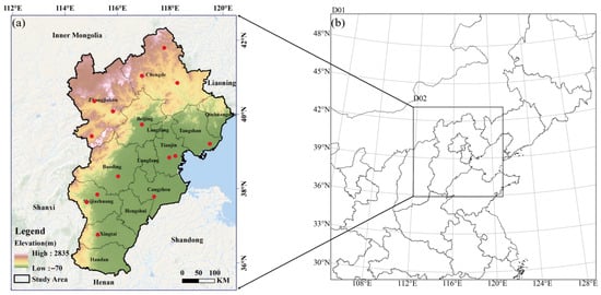
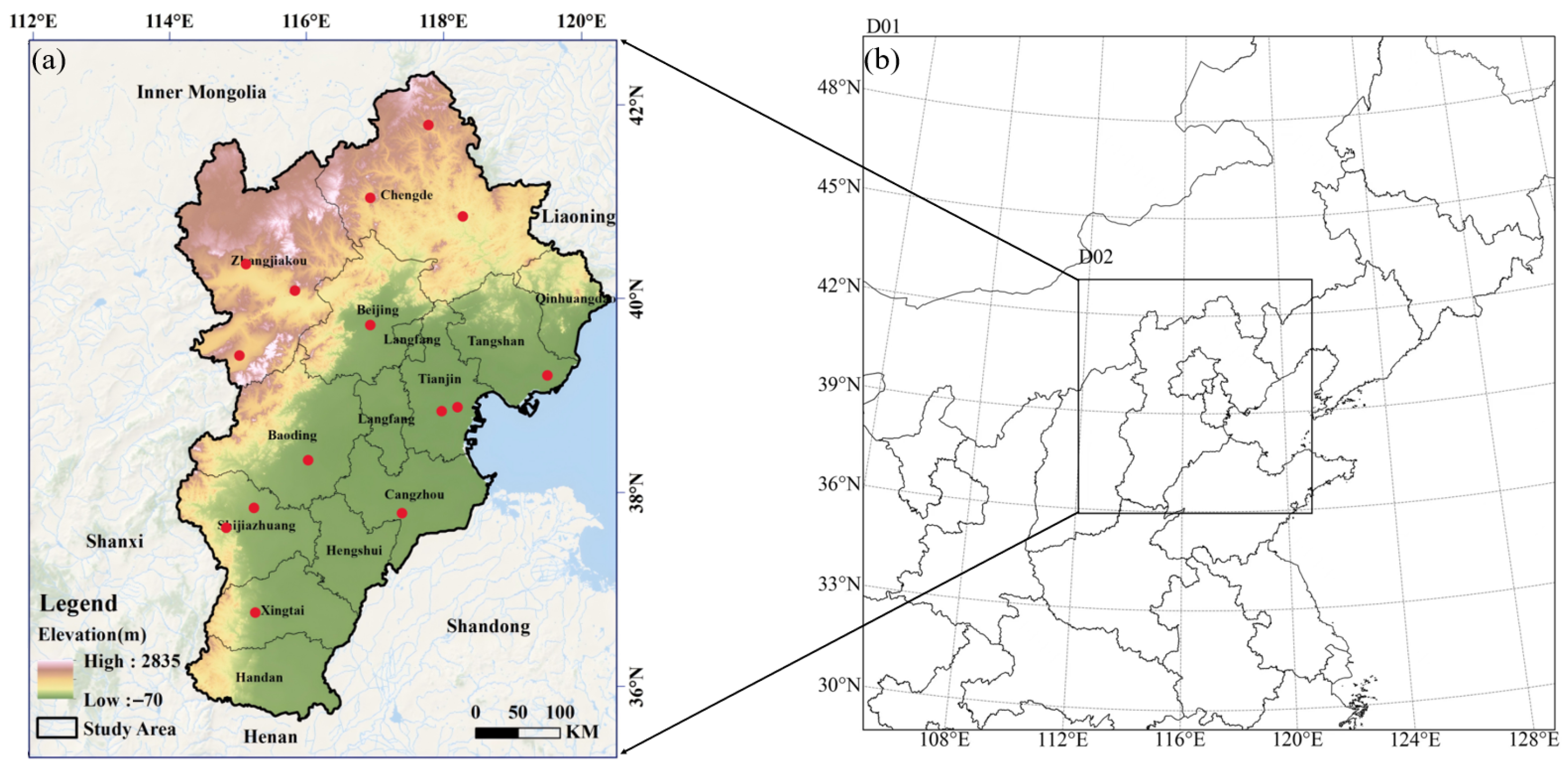
Figure 1a shows the study area in the North China Plain, situated along the eastern coast of China (between longitudes 113° E and 120° E, and latitudes 35° N and 43° N). This area encompasses Beijing, Tianjin, and 11 cities in Hebei Province.

Figure 1. Study area. (a) Topographic overview of the Beijing-Tianjin-Hebei (BTH) region; (b) simulated area. The red dots in (a) indicate the locations of surface meteorological stations. The nested domains D01 and D02 in (b) represent the outer and inner simulation areas of the WRF-Chem model, respectively.

2.2. Observed AOD Data

This study employs the Himawari-8 Level-3 (L3) aerosol product (Version 3.1), which is generated using the enhanced spatiotemporal algorithm developed by Kikuchi et al. [21]. This product has temporal and spatial resolutions of 1 h and 5 km, respectively, and provides AOD data at a wavelength of 500 nm. We specifically employed the AOD_L2_Mean parameter, operated by the Japan Meteorological Agency (JMA) and distributed by the Japan Aerospace Exploration Agency (JAXA) (Tsukuba, Japan), which represents the mean value aggregated from all available Level-2 retrievals within each grid cell over a one-hour interval. To ensure data fidelity, only pixels with high-confidence quality assurance flags (categorized as “good” or “Very good”) were selected for subsequent analysis. After converting the wavelength to 550 nm, AOD data within a radius of 20 km centred around each ground-based meteorological station were extracted as a compromise to achieve both adequate spatial coverage and reliable pixel aggregation, and the average value was considered the AOD value for the station.

2.3. Observed AEC Data

CALIPSO data are categorised into five levels: L0, L1A, L1B, L2, and L3. In this study, the vertical distribution of aerosols was characterized using the CALIPSO Level 2 (L2) 5 km Aerosol Profile product “CAL_LID_L2_05kmAPro”, which provides the AEC at 532 nm. The dataset has a horizontal resolution of 5 km, and the vertical resolution varies with altitude: 60 m from −0.5 to 20.2 km, and 180 m from 20.2 to 30.1 km. Considering that aerosols are mainly concentrated in the boundary layer, only data below 10 km were considered in our analysis.

Rigorous quality control was applied to ensure data reliability. Profiles were retained only if they met all of the following criteria: (1) the CAD_Score was less than −20 (indicating high confidence in aerosol detection); (2) the Extinction_QC_532 flag was 0 or 1 (denoting a valid retrieval with a constrained lidar ratio); and (3) the Atmospheric_Volume_Description confirmed the presence of aerosol (bits 1–3 = 3 and bits 10–12 ≠ 0). Additionally, pixels where the Extinction_Coefficient_532 or its Uncertainty field was flagged as invalid (−9999) were excluded.

2.4. Simulated AEC Data

The WRF-Chem model is a regional chemical transport model, which includes a wide range of physical and chemical parameterizations, enabling accurate representation of atmospheric conditions. It is widely used in air quality modeling applications.

In this study, the model’s initial meteorological fields and lateral boundary conditions are derived from the National Centers for Environmental Prediction (NCEP) Global Forecast System’s Final (FNL) reanalysis data, with a spatial resolution of 1° × 1° and a temporal interval of 6 h. Anthropogenic emissions were sourced from the Multi-resolution Emission Inventory for China (MEIC) developed by Tsinghua University (http://www.meicmodel.org/index.html, accessed on 20 April 2024). The study employs WRF-Chem version 4.1 with a two-nested grid configuration, as shown in Figure 1b. The model is centered at (116.7° E, 39.7° N), with the first grid (D01) having a horizontal resolution of 27 km, covering the North China Plain and northeastern China. The second grid (D02) has a horizontal resolution of 9 km, covering the entire BTH region. The model has 32 vertical layers from the surface to 100 hPa. To accurately resolve vertical aerosol gradients—key for near-surface visibility retrieval—the vertical resolution is finest near the ground. The lowest several layers have thicknesses on the order of 10–20 m, with layer depth increasing approximately logarithmically with height. Given the computational cost and the level of aerosol detail required, the MOSAIC-4bin chemical mechanism [22] is employed to simulate aerosols.

2.5. Surface Visibility Observation Data

The surface visibility observation data from Ground-based meteorological stations within the study area were obtained from the National Oceanic and Atmospheric Administration (NOAA) Global Open Data Repository. To meet user demands for rapid data access and application, NOAA consolidated more than 100 distinct data sources and over 30,000 stations into a comprehensive global archive of surface climate data, known as the Integrated Surface Database (ISD) [23]. VIS data, with 3-hourly measurements, were used to calculate daily average VIS values for stations (marked by red dots in Figure 1) for comparison.

3. VIS Retrieval Method Based on WRF-Chem and CALIPSO

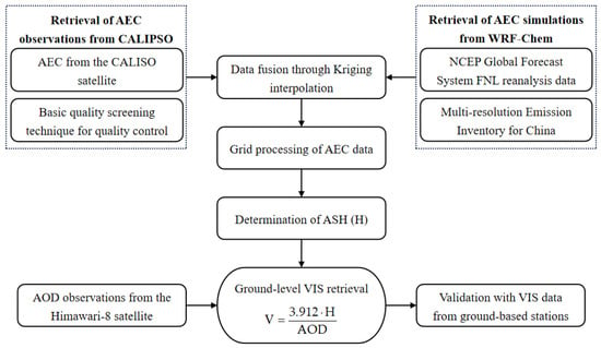
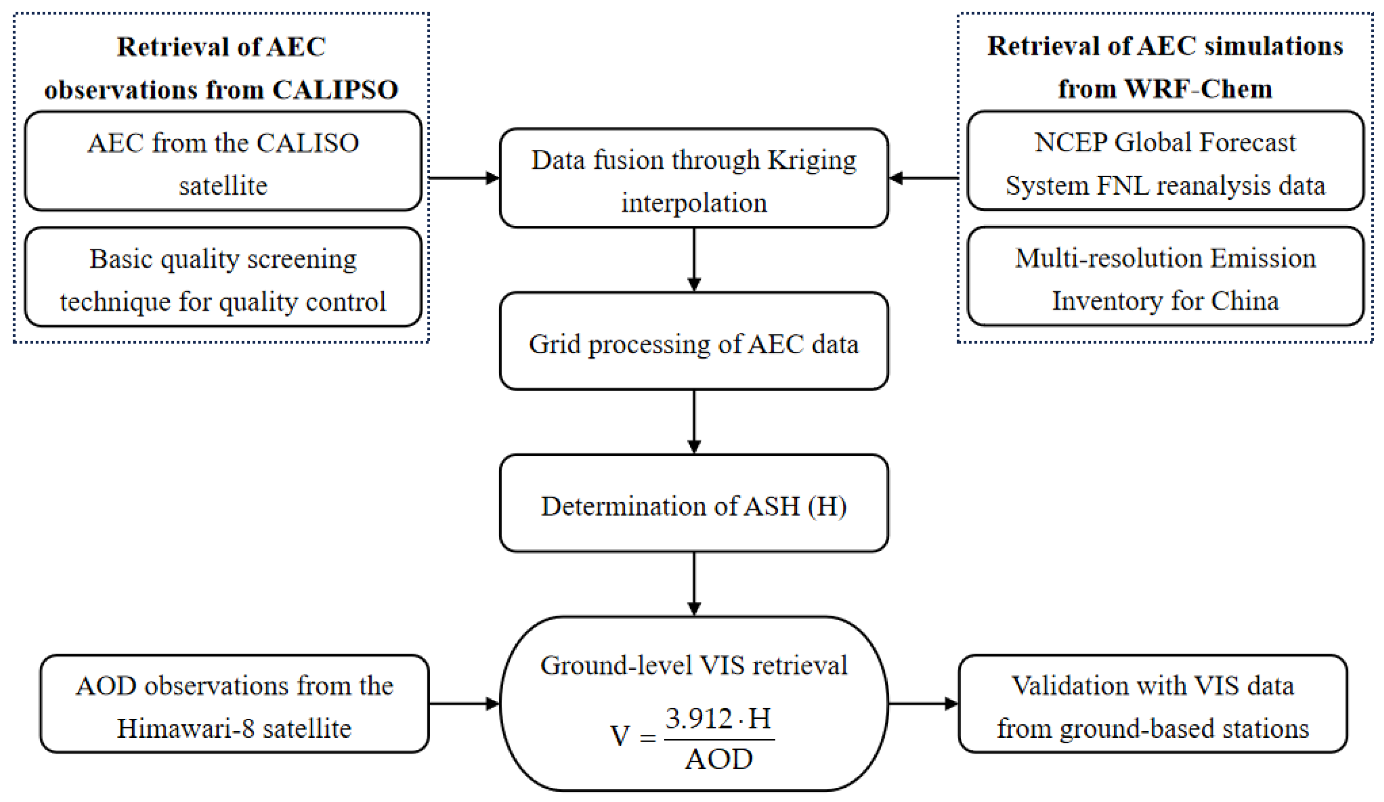
In this study, we propose a novel method for retrieving VIS using observed AEC from CALIPSO, simulated AEC from WRF-Chem, and observed AOD from Himawari-8, as shown in Figure 2. For the first time, Kriging interpolation is applied to fuse CALIPSO and WRF-Chem outputs, ensuring accurate AEC values with high spatial resolution. ASHs under various meteorological conditions are derived from AEC profiles and used for VIS retrieval.

Figure 2. Algorithm process.

3.1. Data Merger Method Based on Kriging Interpolation

Kriging interpolation, a spatial interpolation method based on statistical principles, estimates unknown AEC values by utilizing the spatial correlation between data points and their spatial relationships. This method enables more accurate and intuitive retrieval of AEC distribution at desired geographic coordinates. The estimation process for sampling points is as follows.

$${\widehat{\mathrm{x}}}_0={\displaystyle \sum _{\mathrm{b}=1}^{\mathrm{n}}{\mathrm{w}}_{\mathrm{b}}{\mathrm{x}}_{\mathrm{b}}}$$

(1)

where ${\widehat{\mathrm{x}}}_0$ is the estimated result for the sampling point, $\mathrm{n}$ is the total number of AEC sampling points, ${\mathrm{x}}_{\mathrm{b}}$ is the AEC at a known sampling point, and ${\mathrm{w}}_{\mathrm{b}}$ is the weight assigned to ${\mathrm{x}}_{\mathrm{b}}$, derived from the constraints of unbiased estimation and the optimized objective function. The equations are expressed as

$$\mathrm{E}\left({\widehat{\mathrm{x}}}_0-{\mathrm{x}}_0\right)=0$$

(2)

$$\mathrm{J}=\mathrm{V}\mathrm{a}\mathrm{r}\left({\widehat{\mathrm{x}}}_0-{\mathrm{x}}_0\right)$$

(3)

where $\mathrm{E}$ is the expected value, $\mathrm{J}$ is the optimized objective function, $\mathrm{V}\mathrm{a}\mathrm{r}$ is the variance, and ${\mathrm{x}}_0$ is the true value of ${\widehat{\mathrm{x}}}_0$.

To determine an appropriate data sampling density and accurately represent AEC values in the study area, a semi-variance function is used to assess the spatial correlation between sampling points.

$${\mathrm{r}}_{\mathrm{b}\mathrm{j}}={\displaystyle \frac{1}{2}}\mathrm{E}\left[{\left({\mathrm{x}}_{\mathrm{b}}-{\mathrm{x}}_{\mathrm{j}}\right)}^2\right]$$

(4)

where ${\mathrm{x}}_{\mathrm{j}}$ is the AEC at the ${\mathrm{j}}^{\mathrm{t}\mathrm{h}}$ sampling point within the region, excluding point $\mathrm{b}$. A larger value of ${\mathrm{r}}_{\mathrm{b}\mathrm{j}}$ indicates a stronger degree of correlation between the two variables in space. The expression for weight ${\mathrm{w}}_{\mathrm{b}}$ can be calculated using the following equation.

$$\left[\begin{array}{cccc}{\mathrm{r}}_{11}& {\mathrm{r}}_{12}& \dots & {\mathrm{r}}_{1\mathrm{n}}\\ {\mathrm{r}}_{21}& {\mathrm{r}}_{22}& \dots & {\mathrm{r}}_{2\mathrm{n}}\\ ⋮& ⋮& \ddots & ⋮\\ {\mathrm{r}}_{\mathrm{n}1}& {\mathrm{r}}_{\mathrm{n}2}& \dots & {\mathrm{r}}_{\mathrm{n}\mathrm{n}}\end{array}\right]\left[\begin{array}{c}{\mathrm{w}}_1\\ {\mathrm{w}}_2\\ ⋮\\ {\mathrm{w}}_{\mathrm{n}}\end{array}\right]=\left[\begin{array}{c}{\mathrm{r}}_{10}\\ {\mathrm{r}}_{20}\\ ⋮\\ {\mathrm{r}}_{\mathrm{n}0}\end{array}\right]$$

(5)

During the data interpolation and merger process, based on the AEC values from CALIPSO, the corresponding AEC values from WRF-Chem simulations within 30 m above and below the CALIPSO sampling points are extracted. These are then fused to form the AEC sampling set for this height layer. The Matheron model is used to fit the semi-variance function of the sampling set [24], enabling the determination of the AEC distribution pattern. The equation is expressed as follows.

$$\mathrm{y}\left(\mathrm{h}\right)=\left\{\begin{array}{l}{\mathrm{C}}_0 , \mathrm{h}=0\\ {\mathrm{C}}_0+\mathrm{C}\left({\displaystyle \frac{3\mathrm{h}}{2\mathrm{a}}}+{\displaystyle \frac{{\mathrm{h}}^3}{2{\mathrm{a}}^3}}\right) , 0<\mathrm{h}\le \mathrm{a}\\ {\mathrm{C}}_0+\mathrm{C} , \mathrm{h}>\mathrm{a}\end{array}\right.$$

(6)

where $\mathrm{y}\left(\mathrm{h}\right)$ is the fitted result of the semi-variance function; $\mathrm{h}$ is the distance between any two sampling points; $\mathrm{a}$ is the range threshold, indicating the extent of variation in the variogram in the horizontal direction; ${\mathrm{C}}_0$ is the nugget effect, which represents the variance when the distance is zero and reflects potential spatial variability at very short distances; and ${\mathrm{C}}_0+\mathrm{C}$ is the sill, which is the stable value of the variogram beyond the range and is used to assess the magnitude of regional variable fluctuations.

The same procedure is repeated for the AEC sampling set of each height layer, generating multiple smoothed interpolation surfaces. This results in the AEC distribution for each height layer corresponding to the CALIPSO sampling points in the study area. Subsequently, linear interpolation is applied to transfer the AEC values to uniform grid points, ultimately obtaining the vertical AEC profiles for the ground-based monitoring stations in the study area.

3.2. Basic Principles of VIS Retrieval

Studies have demonstrated that the number concentration of aerosol particles exponentially decreases with height. Assuming that the chemical composition and spectral distribution of aerosol particles remain constant with altitude, the scattering characteristics of these particles depend solely on their number density [25]. Consequently, the variation of the AEC with height can be expressed as

$$\mathrm{\sigma }\left(\mathrm{z}\right)=\mathrm{\sigma }\left(0\right)\exp \left(-{\displaystyle \frac{\mathrm{z}}{\mathrm{H}}}\right)$$

(7)

where $\mathrm{z}$ is the height, $\mathrm{\sigma }\left(\mathrm{z}\right)$ is the AEC at $\mathrm{z}$, and $\mathrm{H}$ is the ASH. AOD can be expressed as the integral of the AEC over a specific vertical layer [26], allowing the total atmospheric AOD to be represented as

$$\mathrm{AOD}={\displaystyle {\int }_0^{\infty }\mathrm{\sigma }\left(\mathrm{z}\right)}\mathrm{d}\mathrm{z}={\displaystyle {\int }_0^{\infty }\mathrm{\sigma }\left(0\right)\exp \left(-\frac{\mathrm{z}}{\mathrm{H}}\right)}\mathrm{d}\mathrm{z}=\mathrm{\sigma }\left(0\right)\mathrm{H}$$

(8)

According to the Koschmieder equation, the relationship between VIS and AEC can be expressed as

$$\mathrm{V}={\displaystyle \frac{-\ln \mathrm{\epsilon }}{\mathrm{\sigma }\left(0\right)}}$$

(9)

where $\mathrm{\epsilon }$ is the threshold of human visual perception, typically set at 0.02. Then, VIS can be expressed as

$$\mathrm{V}={\displaystyle \frac{3.912\cdot \mathrm{H}}{\mathrm{AOD}}}$$

(10)

3.3. Classified ASH Calculation Method

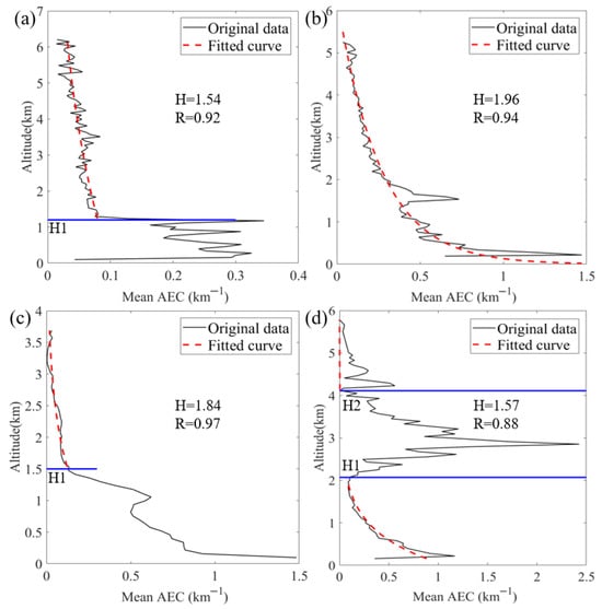
Analysis of AEC vertical distributions under different weather conditions revealed that some profiles follow exponential decay with height, while others do not. Chen et al. [27] also observed varying AEC distributions when calculating AOD using ground-based Lidar and proposed multiple methods for calculating ASH. In this study, we adopted their approach, calculating ASH based on the specific characteristics of different profiles, as shown in Figure 3.

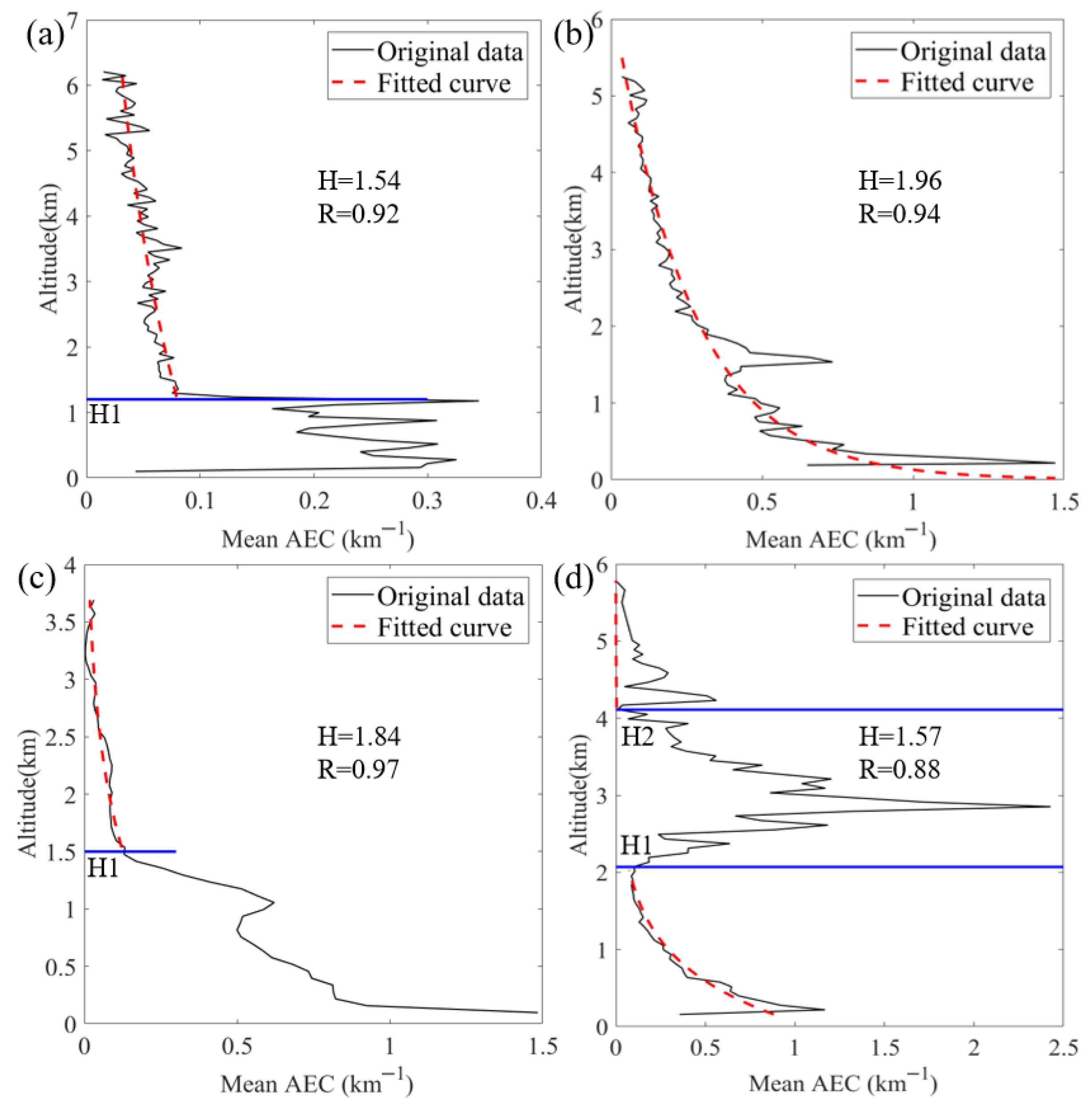
Figure 3. Fitting of different AEC profiles. (a) Uniform base type, (b) exponential decay type, (c) piece-wise decay type, and (d) unimodal type. In all subfigures, H is the ASH and R is the correlation coefficient. The blue lines in (a,c) denote distinct characteristic heights (H1), respectively, representing the top of the uniform layer and the change point in decay rate. In (d), the two blue lines mark the base (H1) and top (H2) of the AEC peak.

In Figure 3a, we observed that the AEC is well-mixed within the boundary layer, whereas an exponential decay occurs above it. For this profile, a piece-wise fitting approach is employed, expressed as follows.

$$\mathrm{\sigma }\left(\mathrm{z}\right)=\left\{\begin{array}{l}\mathrm{\sigma }\left(0\right) , \mathrm{z}<{\mathrm{H}}_1\\ \mathrm{\sigma }\left({\mathrm{H}}_1\right)\exp \left(-{\displaystyle \frac{\left(\mathrm{z}-{\mathrm{H}}_1\right)}{{\mathrm{H}}^{\prime }}}\right) , \mathrm{z}\ge {\mathrm{H}}_1.\end{array}\right.$$

(11)

where ${\mathrm{H}}_1$ is the height of the uniformly mixed aerosol layer, and ${\mathrm{H}}^{\prime }$ is the ASH calculated from the AEC profile that follows the exponential decay. The ASH is determined as $\mathrm{H}={\mathrm{H}}_1+{\mathrm{H}}^{\prime }$. The fit above ${\mathrm{H}}_1$ has a correlation coefficient of 0.92.

In Figure 3b, the AEC profile shows an exponential decay with height, allowing for direct fitting and ASH calculations using Equation (7), resulting in a correlation coefficient of 0.94.

In Figure 3c, due to pollution below a certain height layer, the AEC exhibits inconsistent decay rates across different height layers. A layered fitting approach is also applied to address this issue.

$$\mathrm{\sigma }\left(\mathrm{z}\right)=\left\{\begin{array}{l}\mathrm{\sigma }\left(\mathrm{z}\right) , \mathrm{z}<{\mathrm{H}}_1\\ \mathrm{\sigma }\left({\mathrm{H}}_1\right)\exp \left(-{\displaystyle \frac{\left(\mathrm{z}-{\mathrm{H}}_1\right)}{{\mathrm{H}}^{\prime }}}\right) , \mathrm{z}\ge {\mathrm{H}}_1.\end{array}\right.$$

(12)

To calculate the ASH, the portion above ${\mathrm{H}}_1$ can initially be fitted using an exponential model to obtain $\mathrm{\sigma }\left({\mathrm{H}}_1\right)$ and ${\mathrm{H}}^{\prime }$. The ASH value is determined by dividing the total AOD of both portions by the near-surface AEC, expressed as follows.

$$\mathrm{H}={\displaystyle \frac{\mathrm{\sigma }\left({\mathrm{H}}_1\right){\mathrm{H}}^{\prime }+{\displaystyle {\int }_0^{{\mathrm{H}}_1}\mathrm{\sigma }\left(\mathrm{z}\right)}\mathrm{d}\mathrm{z}}{\mathrm{\sigma }\left(0\right)}}$$

(13)

In Figure 3d, the AEC exhibits a peak at a certain height, with the remaining portion decaying exponentially with height, resulting in a unimodal profile. The variation of the extinction coefficient with height can be expressed as follows.

$$\mathrm{\sigma }\left(\mathrm{z}\right)=\left\{\begin{array}{l}\mathrm{\sigma }\left(0\right)\exp \left(-{\displaystyle \frac{\mathrm{z}}{{\mathrm{H}}^{\prime }}}\right) ,\mathrm{z}<{\mathrm{H}}_1\\ \mathrm{\sigma }\left(\mathrm{z}\right) ,{\mathrm{H}}_1\le \mathrm{z}<{\mathrm{H}}_2\\ \mathrm{\sigma }\left(0\right)\exp \left(-{\displaystyle \frac{\mathrm{z}}{{\mathrm{H}}^{\prime }}}\right) ,\mathrm{z}\ge {\mathrm{H}}_2\end{array}\right.$$

(14)

The ASH ${\mathrm{H}}^{\prime }$ for the portion of the AEC that follows the exponential decay model is first determined. The unimodal portion, when subtracted from the exponentially fitted portion, reflects the outcome resulting from the accumulation of aerosols. The integral of this portion is then calculated, divided by the near-surface AEC, and added to obtain the ASH for the entire aerosol layer, as expressed.

$$\mathrm{H}={\displaystyle \frac{{\displaystyle {\int }_{{\mathrm{H}}_1}^{{\mathrm{H}}_2}\mathrm{\sigma }\left(\mathrm{z}\right)}\mathrm{d}\mathrm{z}-{\displaystyle {\int }_{{\mathrm{H}}_1}^{{\mathrm{H}}_2}\mathrm{\sigma }\left(0\right)}\exp \left(-\frac{\mathrm{z}}{{\mathrm{H}}^{\prime }}\right)\mathrm{d}\mathrm{z}}{\mathrm{\sigma }\left(0\right)}}+{\mathrm{H}}^{\prime }$$

(15)

4. VIS Retrieval Results and Analysis

4.1. AEC Comparison and Merger

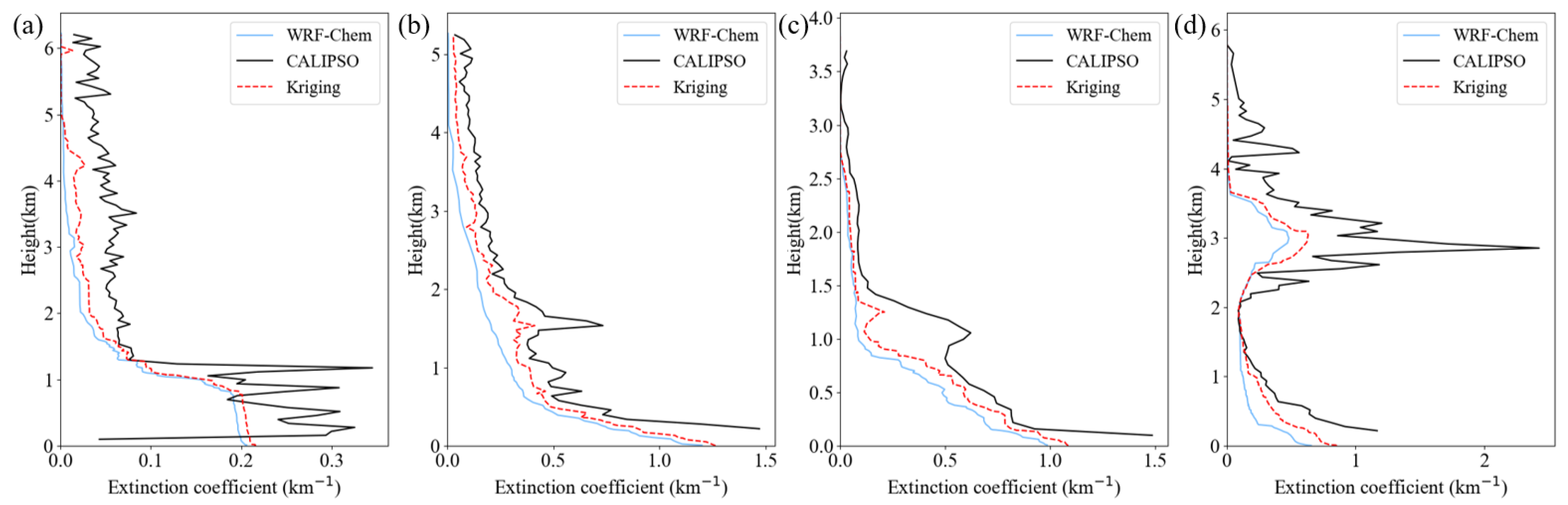
To explore varying meteorological conditions, we selected four weather events: clear weather, sandstorm, haze, and pollution from fireworks. For each event, CALIPSO AEC values were averaged and smoothed. WRF-Chem was used to simulate the three-dimensional aerosol distribution over a three-day period surrounding each event. The simulated AEC values were averaged within a 0.5 h window before and after the satellite’s passage. Figure 4 presents the AEC values from both sources.

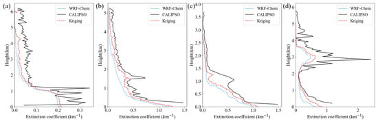
Figure 4. Vertical profiles of AEC. (a) Clear weather, (b) sandstorm, (c) haze, and (d) pollution from the discharge of fireworks and firecrackers.

As shown in Figure 4, AEC values from both data sources exhibit notable correlation under different meteorological conditions, with similar vertical trends. Model simulations are smoother but generally show slightly lower values compared to satellite observations. On 2 August 2020, the study area experienced clear weather with good air quality. Figure 4a shows relatively low AEC values, not exceeding 0.35 km⁻¹, with the highest values near the surface. On 16 April 2021, a spring sandstorm in the BTH region caused a significant increase in AEC, as shown in Figure 4b, with surface values exceeding 1 km⁻¹. On 19 October 2020, during the autumn haze season, Figure 4c shows pollution concentrated below 1.5 km, with AEC above this height approaching zero. The AEC decreased with altitude below 1.5 km, exhibiting higher values near the surface, exceeding 1.4 km⁻¹. While there are slight discrepancies between model simulations and satellite observations, the overall trends are consistent. On 25 January 2020, during the Chinese Lunar New Year, fireworks increased aerosol concentrations, exacerbated by high-pressure weather conditions, leading to a typical pollution episode [28]. Figure 4d shows an elevated AEC near the surface, with a peak around 3 km, likely due to multi-scale atmospheric processes. During the daytime on New Year’s Eve, fireworks-emitted aerosols were well-mixed within the convective boundary layer. After sunset, surface radiative cooling established a stable nocturnal boundary layer that suppressed vertical diffusion near the surface. However, a significant portion of the previously elevated aerosols remained aloft in the residual layer above. Winds within the residual layer are often stronger, enabling horizontal long-range transport of these aerosols. Additionally, the launch height of large professional fireworks, the collective thermal buoyancy from intensive burning, and potential gas-phase secondary aerosol formation during transport may have contributed to the elevated aerosol layer.

Considering the nonlinear distribution of AEC across height layers, three metrics—correlation coefficient (CORR, representing the goodness-of-fit between simulated and observed AEC profiles), root mean square error (RMSE), and mean fractional error (MFE)—are used to quantify the improvement in AEC simulation by integrating CALIPSO data. The formulas for these metrics are provided, where S, O, and N represent the simulated results, observed results, and the number of samples, respectively. The results are shown in Table 1.

$$\mathrm{C}\mathrm{O}\mathrm{R}\mathrm{R}={\displaystyle \frac{{\displaystyle \sum _{\mathrm{i}=1}^{\mathrm{N}}\left({\mathrm{S}}_{\mathrm{i}}-\overline{\mathrm{S}}\right)}\cdot \left({\mathrm{O}}_{\mathrm{i}}-\overline{\mathrm{O}}\right)}{\sqrt{{\displaystyle \sum _{\mathrm{i}=1}^{\mathrm{N}}{\left({\mathrm{S}}_{\mathrm{i}}-\overline{\mathrm{S}}\right)}^2}}\cdot \sqrt{{\displaystyle \sum _{\mathrm{i}=1}^{\mathrm{N}}{\left({\mathrm{O}}_{\mathrm{i}}-\overline{\mathrm{O}}\right)}^2}}}}$$

(16)

$$\mathrm{R}\mathrm{M}\mathrm{S}\mathrm{E}=\sqrt{{\displaystyle \frac{1}{\mathrm{N}}}{\displaystyle \sum _{\mathrm{i}=1}^{\mathrm{N}}{\left({\mathrm{S}}_{\mathrm{i}}-{\mathrm{O}}_{\mathrm{i}}\right)}^2}}$$

(17)

$$\mathrm{M}\mathrm{F}\mathrm{E}={\displaystyle \frac{1}{\mathrm{N}}}{\displaystyle \sum _{\mathrm{i}=1}^{\mathrm{N}}\left|\frac{{\mathrm{S}}_{\mathrm{i}}-{\mathrm{O}}_{\mathrm{i}}}{\left({\mathrm{S}}_{\mathrm{i}}+{\mathrm{O}}_{\mathrm{i}}\right)/2}\right|}$$

(18)

Table 1. AEC error analysis before and after interpolation.

Weather Conditions	WRF-Chem Simulation			Kriging Interpolation
	CORR	RMSE	MFE	CORR	RMSE	MFE
Clear	0.86	0.06	0.48	0.89	0.05	0.32
Sandstorm	0.95	0.18	0.74	0.97	0.12	0.41
Haze	0.91	0.20	0.86	0.93	0.15	0.45
Fireworks	0.83	0.44	0.96	0.82	0.38	0.54
Mean	0.89	0.22	0.76	0.90	0.18	0.43

All three metrics improved under the four meteorological conditions, with the highest correlation observed during dust weather. This enhancement is likely due to the distinct particle characteristics of dust, where the extinction coefficient follows an exponential decay. The proposed algorithm effectively addresses model uncertainties in such conditions. For fireworks and firecracker conditions, the CORR slightly decreased, likely due to the complex nature of fireworks particles. However, both the RMSE (from 0.44 to 0.38) and MFE (from 0.96 to 0.54) showed significant improvement, demonstrating the method’s effectiveness.

4.2. ASH Calculation and Point-to-Point VIS Comparison

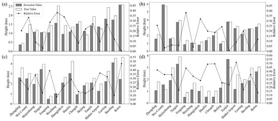
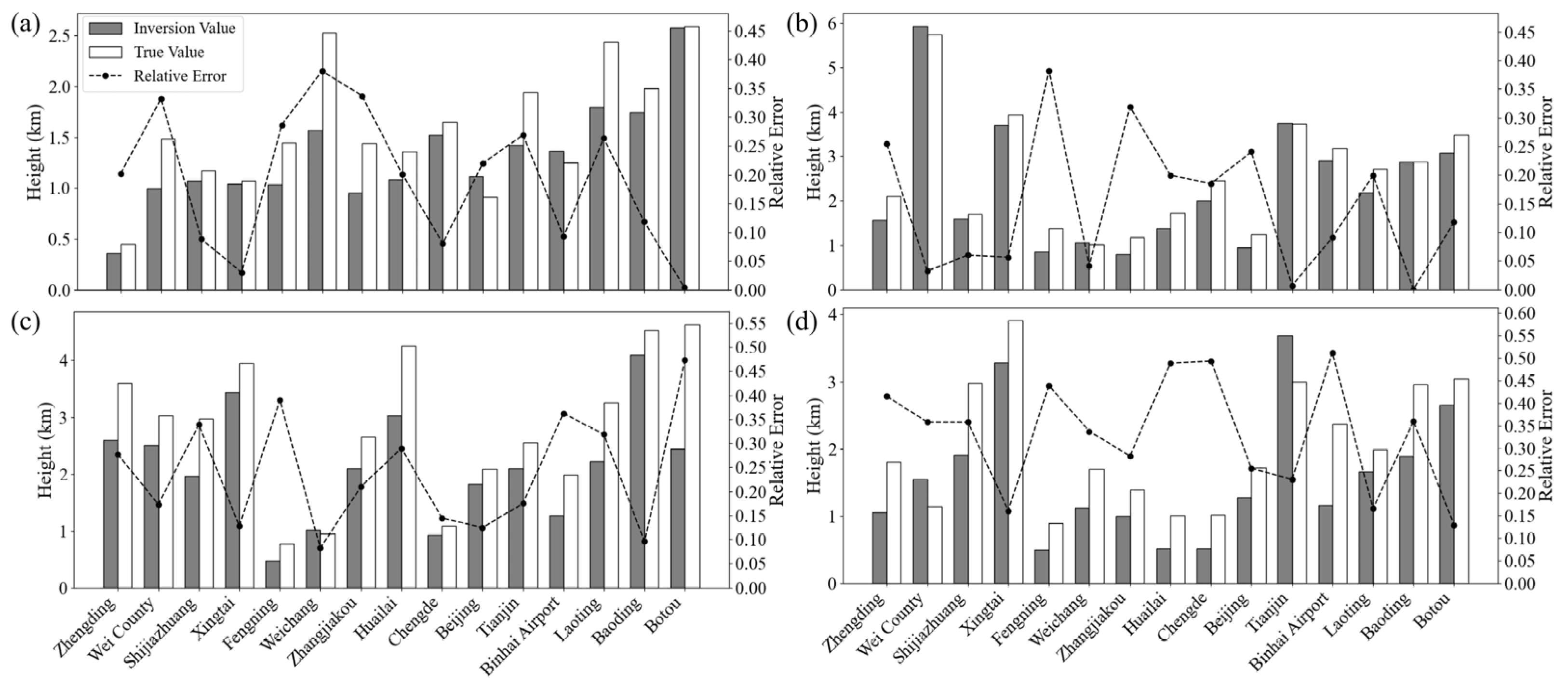
When analyzing the retrieval of ASH values, the VIS observations from the ground-based meteorological stations were regarded as accurate values, from which the true ASH values were calculated using Equation (10). By applying the ASH calculation method outlined in Section 3.3 and utilizing the interpolated AEC profiles, the retrieved ASH values for 15 stations within the study area were calculated. These values are compared with the true values, as shown in Figure 5.

Figure 5. Point-to-point comparison of ASHs. (a) Clear weather, (b) sandstorm, (c) haze, and (d) discharge of fireworks and firecrackers. In all subplots, “True value” refers to the ASH calculated using Equation (10) under the assumption that the surface visibility observed at meteorological stations is accurate, while “Inversion value” denotes the ASH derived by applying the retrieval method described in Section 3.3 to the interpolated aerosol extinction coefficient profiles.

As shown in Figure 5, the ASH retrieval values align well with the true values across different meteorological conditions. Under clean weather, the average relative error is 19%, with a minimum of 8%, confirming the reliability of the ASH method. For light pollution conditions (e.g., dust and haze), the average relative error is around 24%. Even during more polluted events like fireworks, the error can be as low as 13%, with an average of 30%. These results highlight the algorithm’s robustness. Figure 6 compares the atmospheric VIS derived from the retrieved ASH values with ground-based observations.

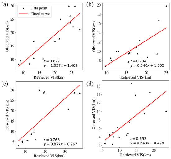
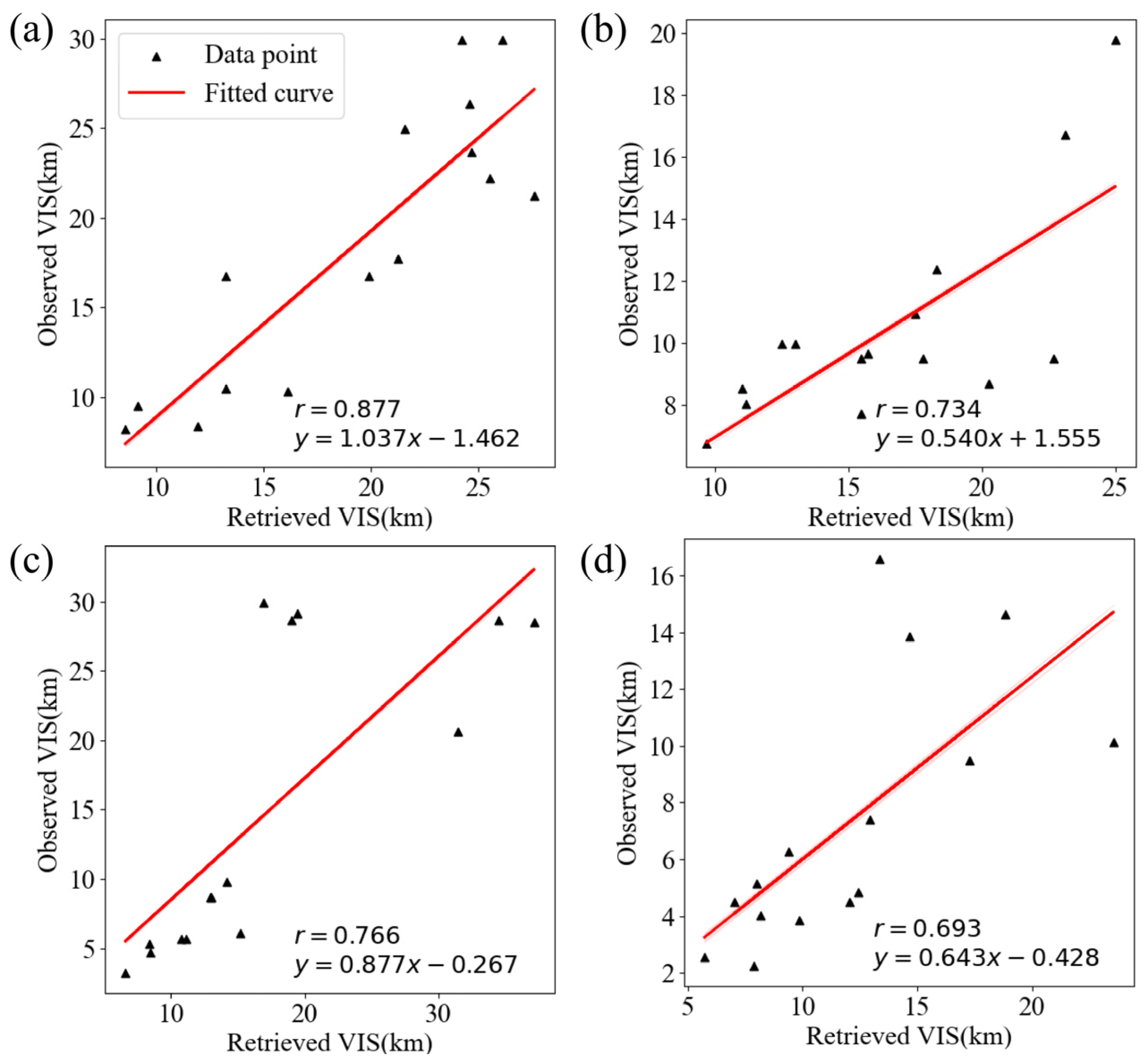
Figure 6. Retrieved VIS. (a) Clear weather, (b) sandstorm. (c) haze, and (d) discharge of fireworks and firecrackers.

The CORR between the retrieved and observed VIS ranges from 0.69 to 0.87, which directly measures the algorithm’s accuracy, showing generally favorable retrieval results. The highest CORR of 0.87 occurs under clear weather, where low aerosol concentrations and uniform distribution allow satellite-derived AOD to effectively reflect ground-level VIS. In sandstorms and haze, the CORR is 0.73 and 0.76, respectively, as higher aerosol concentrations and more complex atmospheric compositions complicate ASH calculation and AOD-to-VIS conversion. For fireworks-induced pollution, the CORR drops to 0.69 due to high aerosol concentrations, complex compositions, and intricate optical and vertical distribution characteristics. Chen et al. [27] also noted that the ASH fitting method’s accuracy diminishes under severe pollution, contributing to larger visibility retrieval errors.

Across different meteorological conditions, the retrieval algorithm proposed in this study exhibits robust performance, providing valuable insights for atmospheric research and VIS observation. The experimental findings highlight the importance of carefully considering both meteorological factors and the vertical distribution of aerosols when conducting VIS retrievals to improve the accuracy of the results.

5. Discussion

5.1. Interpreting Retrieval Performance Across Weather Scenarios

The point-to-point validation yielded CORR values ranging from 0.69 to 0.87. This range confirms that weather type is a critical factor influencing retrieval performance, with results showing a distinct stratification across the scenarios studied. The variation is fundamentally attributed to the differing degrees of complexity in aerosol loading, vertical distribution, and the associated uncertainties in both satellite remote sensing and chemical transport modeling for each scenario.

Clear conditions (CORR = 0.87) exhibited the highest accuracy. This superior performance stems primarily from low and horizontally homogeneous aerosol loading. Under such ideal circumstances, the foundational assumptions of satellite AOD retrieval algorithms and chemical transport models are most valid, resulting in minimal errors in both the AOD input data and the simulated vertical profiles. Consequently, this allows for a more accurate estimation of the Aerosol Scale Height (ASH) and a more reliable conversion to visibility.

Sandstorm events (CORR = 0.73) showed robust but moderated performance. Although the aerosol vertical profile in such events often approximates an exponential decay—which is favorable for ASH fitting—retrieval accuracy is constrained by challenges intrinsic to dust aerosols. Key among these are the uncertainties in dust optical properties (e.g., due to non-sphericity and variable refractive index) and potential inaccuracies in the model’s dust emission and transport schemes. These factors introduce errors that propagate into the fused aerosol extinction coefficient (AEC) field.

Haze episodes (CORR = 0.76) presented greater complexity, leading to a noticeable decline in correlation. This performance drop reflects the intricate nature of fine particulate pollution. Aerosols during haze are frequently dominated by hygroscopic species, whose size and extinction efficiency increase with humidity. Furthermore, haze conditions often coincide with stable atmospheric stratification and a shallow boundary layer, which challenge the model’s ability to accurately simulate the vertical confinement and concentration of pollutants near the surface.

Fireworks pollution (CORR = 0.69) posed the most significant challenge, as evidenced by the lowest CORR. The errors are attributed to a confluence of factors: (a) the unique, elevated unimodal vertical structure (with a peak near 3 km) starkly deviates from conventional decay assumptions; (b) the aerosol composition is chemically complex and transient, lacking well-defined optical parameters in standard models; and (c) the intense, highly localized emission sources are difficult for a regional-scale model like WRF-Chem to capture precisely. These elements collectively amplify the uncertainties in both the ASH derivation and the final AOD-to-visibility conversion.

5.2. Limitations and Future Perspectives

It is important to note a key limitation of the current validation dataset: the number of observed very low-visibility samples was scarce within the selected case studies. Nonetheless, the fireworks and haze cases, representing our relatively lowest visibility events, provide valuable qualitative insights. The increased errors in these scenarios are likely tied to the heightened sensitivity of the AOD-to-visibility conversion to aerosol microphysical properties (e.g., hygroscopic growth in haze, composition of firework plumes) under high loading conditions, which are not fully captured by the current generalized ASH parameterization. Future work must prioritize expanding the validation dataset to include more extreme low-visibility cases to properly address this gap.

Furthermore, a systematic low bias was observed in WRF-Chem simulated AEC compared to satellite observations, suggesting that implementing dynamic bias correction could mitigate this discrepancy. Enhancing the resolution of the meteorological initial and boundary conditions would also improve the model’s accuracy in simulating vertical pollutant transport. Regarding spatial representativeness, the current framework employs a 20 km radius to aggregate satellite AOD, which is suitable for regional-scale retrieval but may smooth out localized features critical for point-specific applications like aviation. To bridge this gap, future research should test the sensitivity of retrievals to smaller spatial scales and explore the integration of higher-resolution, localized data sources to better capture fine-scale visibility variations near critical infrastructure such as airports. Looking forward, translating this general-purpose retrieval framework into operational tools constitutes a logical next step. This would entail application-specific adaptations, such as recalibration using the ICAO standard contrast threshold (ε = 0.05) for aviation, incorporating aerosol-type-specific optical parameters, and rigorous validation against categorical observations.

6. Conclusions

This study developed a novel surface visibility retrieval framework by constructing a high-resolution extinction field through Kriging-based fusion of CALIPSO vertical profiles and WRF-Chem simulations, combined with Himawari-8 AOD data. The research confirms that accurately characterizing the vertical distribution of aerosols is key to improving retrieval precision. By classifying AEC profiles into multiple types to dynamically estimate the ASH, the method effectively overcomes the limitations of traditional approaches that rely on constant ASH or simplified exponential decay assumptions. The framework demonstrates robust applicability across diverse weather conditions, achieving correlation coefficients between retrieved and ground-observed visibility of 0.69–0.87 under four typical scenarios. Meanwhile, error analysis during complex pollution episodes points the way for future refinement, as cases such as haze and fireworks reveal that incorporating aerosol-type-specific optical parameters and hygroscopicity corrections will be essential for further optimizing algorithm performance. It should be noted that while CALIPSO data are crucial for developing and validating the fusion algorithm in this study, the envisioned near-real-time operational application would primarily rely on the high-frequency Himawari-8 observations and WRF-Chem forecast fields, without the need for concurrent CALIPSO overpasses. In summary, this work provides a reliable technical framework for high-accuracy, operational regional visibility monitoring and lays a methodological foundation for developing specialized meteorological services in fields such as aviation safety.

References

- Watson, J.G. Visibility: Science and regulation. J. Air Waste Manag. Assoc. 2002, 52, 628–713. [Google Scholar] [CrossRef] [Scilit] [PubMed]
- Kulkarni, R.; Jenamani, R.K.; Pithani, P.; Konwar, M.; Nigam, N.; Ghude, S.D. Loss to Aviation Economy Due to Winter Fog in New Delhi during the Winter of 2011–2016. Atmosphere 2019, 10, 198. [Google Scholar] [CrossRef] [Scilit]
- Zhou, S.D.; Ma, Z. Influence of optical path collimation on measurement of long baseline transmission visibility meter. J. Appl. Opt. 2016, 37, 87–90. [Google Scholar]
- Sun, J.; Shu, J.; Lu, X.Q.; Duan, Y.S.; Chen, J.P. Shanghai aerosol characteristics and application of MODIS aerosol product to retrieval visibility. Environ. Pollut. Control 2007, 29, 5. (In Chinese) [Google Scholar]
- Zhang, H.; Deng, X.L.; Shi, C. Application of MODIS aerosol products in monitoring visibility. Environ. Sci. Technol. 2015, 38, 7. (In Chinese) [Google Scholar]
- Tan, Y.H.; Wang, Q.; Zhang, Z.Y. Assessing spatiotemporal variations of AOD in Japan based on Himawari-8 L3 V31 aerosol products: Validations and applications. Atmos. Pollut. Res. 2022, 13, 101439. [Google Scholar] [CrossRef] [Scilit]
- Tang, C.; Shi, C.; Letu, H.; Yin, S.; Nakajima, T.; Sekiguchi, M.; Xu, J.; Zhao, M.; Ma, R.; Wang, W. Development of a hybrid algorithm for the simultaneous retrieval of aerosol optical thickness and fine-mode fraction from multispectral satellite observation combining radiative transfer and transfer learning approaches. Remote Sens. Environ. 2025, 319, 114619. [Google Scholar] [CrossRef] [Scilit]
- Xu, L.X.; Fei, Y.; Li, L.L. Inverse calculation of visibility in Henan Province based on Hiwamari-8 satellite AOD products. J. Shaanxi Meteorol. 2020, 36–41. (In Chinese) [Google Scholar] [CrossRef]
- Zhang, Y.; Han, Y. Direct measurement techniques for atmospheric aerosol: Optical and chemical properties review. Sci. China Earth Sci. 2025, 68, 3454–3481. [Google Scholar] [CrossRef] [Scilit]
- Winker, D.M.; Tackett, J.L.; Getzewich, B.J.; Liu, Z.; Vaughan, M.A.; Rogers, R.R. The global 3-D distribution of tropospheric aerosols as characterized by CALIOP. Atmos. Chem. Phys. 2013, 13, 3345–3361. [Google Scholar] [CrossRef] [Scilit]
- Penndorf, R.B. The Vertical Distribution of Mie Particles in the Troposphere. J. Atmos. Sci. 1954, 11, 245–247. [Google Scholar] [CrossRef] [Scilit]
- Sun, X.J.; Zhou, Y.B.; Zhang, R.W.; Zhou, J.H.; Li, H.R. Influences of extinction coefficient profile on the estimation of Slant Visual Range. Atmos. Environ. 2015, 122, 484–492. [Google Scholar] [CrossRef] [Scilit]
- Yang, T.; Li, J.; Wang, Z.; Zhang, Z.; Wang, X.; Gbaguidi, A. Vertical Distribution of the Aerosol Optical Characteristics during the 2008 Beijing Olympic Games. Clim. Environ. Res. 2010, 15, 602–608. [Google Scholar]
- Lin, J.T.; van Donkelaar, A.; Xin, J.Y.; Che, H.Z.; Wang, Y.S. Clear-sky aerosol optical depth over East China estimated from visibility measurements and chemical transport modeling. Atmos. Environ. 2014, 95, 258–267. [Google Scholar] [CrossRef] [Scilit]
- Zang, Z.L.; You, W.; Ye, H.C.; Liang, Y.F.; Li, Y.; Wang, D.C.; Hu, Y.W.; Yan, P. 3DVAR Aerosol Data Assimilation and Evaluation Using Surface PM2.5, Himawari-8 AOD and CALIPSO Profile Observations in the North China. Remote Sens. 2022, 14, 4009. [Google Scholar] [CrossRef] [Scilit]
- Zhang, Y.; Li, J. Retrieval of surface visibility using satellite-based aerosol measurements. Acta Sci. Nat. Univ. Pekin. 2020, 56, 231–241. (In Chinese) [Google Scholar]
- Zhou, Z.H.; Liu, Y.L.; Zhang, W.J.; Fu, R. Surface Visibility Retrieval with Observations from the Medium Resolution Spectral Imager (MERSI) Onboard the FY-3A Meteorological Satellite. AIP Conf. Proc. 2013, 1531, 396–399. [Google Scholar] [CrossRef] [Scilit]
- Wang, M.; Yu, J.; Bai, L.; Zhou, Y. Optical properties of ensemble of complex externally mixed aerosol particles under different relative humidity conditions. Acta Phys. Sin. 2025, 74, 064203. [Google Scholar] [CrossRef] [Scilit]
- Chen, J.J.; Sheng, L.F.; Zheng, Y.X. The correlation analysis of aerosol optical depth, aerosol index and visibility in Qingdao spring 2006. Period. Ocean Univ. China (Nat. Sci. Ed.) 2010, 40, 10–16. (In Chinese) [Google Scholar]
- Zong, P.; Zhu, Y.; Wang, H.; Liu, D. WRF-Chem simulation of winter visibility in Jiangsu, China, and the application of a neural network algorithm. Atmosphere 2020, 11, 520. [Google Scholar] [CrossRef] [Scilit]
- Kikuchi, M.; Murakami, H.; Suzuki, K.; Nagao, T.M.; Higurashi, A. Improved Hourly Estimates of Aerosol Optical Thickness Using Spatiotemporal Variability Derived from Himawari-8 Geostationary Satellite. IEEE Trans. Geosci. Remote Sens. 2018, 56, 3442–3455. [Google Scholar] [CrossRef]
- Zaveri, R.A.; Easter, R.C.; Fast, J.D.; Peters, L.K. Model for Simulating Aerosol Interactions and Chemistry (MOSAIC). J. Geophys. Res. Atmos. 2008, 113, 29. [Google Scholar] [CrossRef] [Scilit]
- Smith, A.; Lott, N.; Vose, R. The Integrated Surface Database: Recent Developments and Partnerships. Bull. Am. Meteorol. Soc. 2011, 92, 704–708. [Google Scholar] [CrossRef] [Scilit]
- Matheron, G. Principles of geostatistics. Econ. Geol. 1963, 58, 1246–1266. [Google Scholar] [CrossRef] [Scilit]
- Ding, H.X. Lidar Observations of Tropospheric Aerosols in the Urban Area of Suzhou. Master’s Thesis, Soochow University, Suzhou, China, 2004. (In Chinese) [Google Scholar]
- Coakley, J.A., Jr.; Yang, P. Atmospheric Radiation: A Primer with Illustrative Solutions; Wiley-VCH: Berlin, Germany, 2014; pp. 81–82. [Google Scholar]
- Chen, S.S.; Xu, Q.S.; Xu, C.D.; Yu, D.S.; Chen, X.W. Calculation of whole atmospheric aerosol optical depth based on micro-pulse Lidar. Acta Opt. Sin. 2017, 37, 9. (In Chinese) [Google Scholar] [CrossRef] [Scilit]
- Gao, Q.X.; Wang, N.; Gao, W.K.; Gao, W.O.; Li, Y.X.; Fu, J.F.; Dai, J.Q. Analysis of two atmospheric heavy pollution processes in Beijing-Tianjin-Hebei and surrounding areas during the Spring Festival of 2020. J. Environ. Eng. Technol. 2020, 10, 14. (In Chinese) [Google Scholar]
Disclaimer/Publisher’s Note: The statements, opinions and data contained in all publications are solely those of the individual author(s) and contributor(s) and not of MDPI and/or the editor(s). MDPI and/or the editor(s) disclaim responsibility for any injury to people or property resulting from any ideas, methods, instructions or products referred to in the content. |
© 2026 by the authors. Licensee MDPI, Basel, Switzerland. This article is an open access article distributed under the terms and conditions of the Creative Commons Attribution (CC BY) license.