


Abstract
Forecasting post-seismic landslide displacement is challenged by the difficulty in distinguishing short-term acceleration from creep and the risk of spatiotemporal leakage. To address this, an interpretable deep-learning framework is developed, integrating SBAS-InSAR time series with an Attention-enhanced Gated Recurrent Unit (Attention-GRU). Prior to modeling, a multi-stage preprocessing strategy, including empirical mode decomposition, is applied to mitigate noise and delineate active deformation zones. Unlike standard architectures, the model’s temporal attention mechanism adaptively amplifies critical precursory acceleration phases. Furthermore, a strict landslide-object-based partitioning strategy is employed to rigorously mitigate spatiotemporal leakage. The framework was evaluated in the Le’an Town landslide cluster using multi-source data. Targeting identified hazardous regions, the method achieved an R2 of 0.93 and reduced MAPE by 42.7% relative to the SVR baseline. This reflects a location-specific predictive capability, within active zones rather than regional generalization. SHapley Additive exPlanations (SHAP) further confirmed the model captures physical relationships, such as sensitivity to 25–35° slopes and vegetation degradation. Ultimately, the proposed framework offers a transparent, physically interpretable tool for operational hazard mitigation.
1. Introduction
Landslides in seismically active mountainous regions represent complex geomorphic systems driven by the nonlinear coupling of internal geological damage and external hydrometeorological triggers [1,2,3]. This complexity is particularly pronounced in post-seismic environments, where earthquake-induced rock mass shattering leaves slopes in a state of heightened susceptibility for decades, as evidenced by long-term observations following the 2008 Wenchuan and 2013 Ya’an earthquakes [4,5,6]. In these fragile landscapes, the “post-seismic effect” creates a hazard environment characterized by delayed deformation, extensive ground fracturing, and persistent sediment supply [7,8,9]. While the socioeconomic impact of these geohazards is profound, the scientific challenge lies in accurately predicting the temporal onset of catastrophic failure. Reliable forecasting requires capturing the subtle transition from steady-state creep to rapid acceleration, a task complicated by the inherent nonlinearity of deformation trajectories and the diverse lag effects of environmental drivers such as extreme rainfall [10,11,12] and vegetation degradation [13,14].
To monitor these inaccessible and high-risk terrains, Space-borne Interferometric Synthetic Aperture Radar (InSAR), particularly the Small Baseline Subset (SBAS) technique, has become the standard for reconstructing historical surface deformation with millimeter-level precision [15,16,17]. Recent applications have further expanded the utility of SBAS-InSAR beyond simple monitoring, demonstrating its efficacy in mapping subsidence susceptibility in tectonically active zones [18,19], extracting hydro-mechanical parameters for slope stability models [20,21], and identifying broad-scale deformation patterns [22]. However, a critical gap persists between retrospective monitoring and prospective forecasting: InSAR products are descriptive by nature, documenting past displacement, whereas early warning requires predictive models capable of extrapolating future states. To bridge this gap, recent advancements have increasingly integrated InSAR time series with deep learning architectures, such as Gated Recurrent Units (GRU) and Long Short-Term Memory (LSTM) networks [23,24,25]. These models have demonstrated superior capability in capturing sequential dependencies compared to traditional static regression methods (e.g., SVR, Random Forest), offering a promising pathway for data-driven hazard mitigation [26,27,28].
Despite the proliferation of deep learning applications in landslide forecasting, the operational validity of current frameworks faces certain architectural and methodological challenges. A limitation in standard recurrent models is their tendency to assign uniform computational importance to all historical time steps [29,30]. This design may not fully align with the kinematic reality of slope failure, where short-term acceleration phases contain disproportionately higher precursory value than prolonged quiescent periods, potentially leading to the dilution of critical warning signals [31,32]. While attention mechanisms have been introduced to address this temporal weighting issue, a conceptual and operational gap remains regarding how these models are validated within complex spatial environments. Compounding this is the lack of mechanistic transparency in multi-source fusion strategies. Environmental variables are frequently integrated via direct feature concatenation, which may obscure physical coupling mechanisms, such as root reinforcement or stress concentration. Perhaps the most pervasive yet under-discussed issue concerns the validation protocols employed for data-driven models. The majority of existing studies, including many utilizing advanced attention modules, utilize random data partitioning, where samples from the same landslide body are arbitrarily split between training and testing sets. As highlighted by recent critiques, this practice introduces potential spatiotemporal information leakage, allowing models to memorize spatial autocorrelations rather than generalizing deformation patterns [33,34]. Consequently, models that achieve exceptionally high accuracy metrics in experimental settings may face challenges when applied to spatially unseen slopes. Therefore, our methodology fundamentally differs from existing attention-based InSAR approaches by integrating the attention mechanism within a rigorous spatiotemporal partitioning framework, ensuring the model learns robust precursory features rather than memorizing spatial leakage.
To transcend these limitations, this research establishes an interpretable deep learning framework that couples SBAS-InSAR time-series analysis with an Attention-enhanced Gated Recurrent Unit (Attention-GRU). Distinct from conventional approaches, the proposed architecture integrates an adaptive temporal attention mechanism designed to dynamically amplify the weights of critical acceleration phases preceding instability, thereby aligning the model’s focus with the kinematic characteristics of landslide evolution. Addressing the issue of data leakage, a strict landslide-object-based partitioning strategy is implemented. By isolating training and testing datasets by spatial units, this protocol ensures that the model is evaluated on its ability to generalize to new geological entities, providing a realistic assessment of operational transferability. Furthermore, this study moves beyond accuracy metrics to validate the physical consistency of the model. Through SHapley Additive exPlanations (SHAP) dependence analysis, the framework quantifies the marginal contributions of geomorphic drivers, verifying whether the learned relationships, such as the nonlinear sensitivity to slope gradients or the destabilizing effects of vegetation degradation, conform to established rock mechanics theories. Validated in the Le’an Town landslide cluster, a representative post-seismic region, this work aims to transform landslide displacement forecasting from an opaque regression task into a transparent, physically interpretable diagnostic tool suitable for robust early warning applications.
2. Materials and Methods
2.1. Study Area and Data Sources
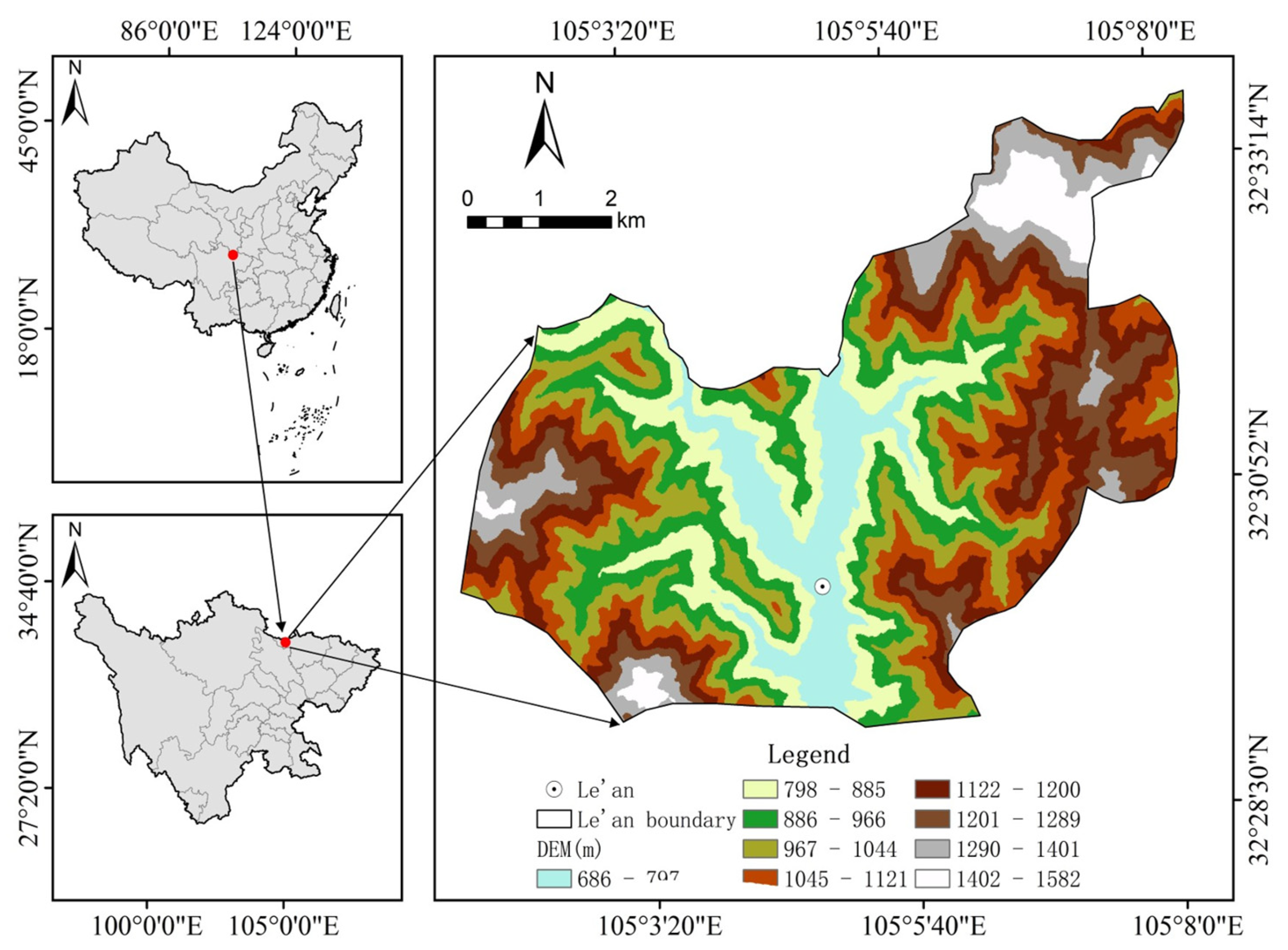
Le’an Town (32°30′–32°33′ N, 105°03′–105°08′ E), situated within Guangyuan City, Sichuan Province, represents a typical high-risk geological environment in Southwestern China (Figure 1). Located at the tectonic junction of the Longmen and Micang Mountain ranges, the region is characterized by dramatic topographic relief and complex geological structures. This area is not only influenced by long-term tectonic activities, evidenced by the extensive ground deformation following the 2008 Wenchuan (Mw 7.9) and 2013 Ya’an (Mw 6.6) earthquakes, but is also significantly driven by seasonal climatic factors. This post-seismic setting provides an ideal testbed for validating data-driven models, as recent global assessments demonstrate the superior capacity of deep-learning frameworks in characterizing earthquake-triggered landslide susceptibility and evolution [35].
Figure 1.
Location map of the study area.
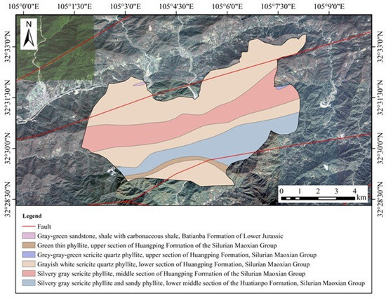
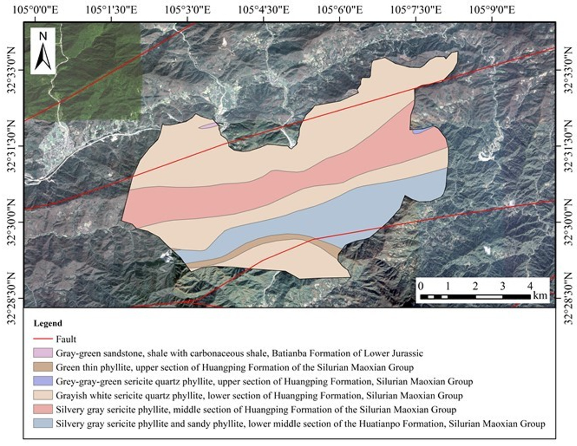
The lithological setting is highly heterogeneous, comprising karst-dominated Paleozoic limestone interbedded with tectonically fractured Mesozoic slate (Figure 2), which creates a fragile substrate prone to instability. To scientifically quantify the environmental context of landslide development, multi-dimensional spatio-temporal features including topographic slope, aspect, surface roughness, and the Normalized Difference Vegetation Index (NDVI), were extracted and analyzed. Statistical assessments indicate that active landslides exhibit significant spatial clustering, particularly in steep sectors with gradients ranging from 25° to 40°. Furthermore, deformation rates show a distinct non-linear correlation with rainfall-induced NDVI fluctuations, suggesting that vegetation dynamics serve as a proxy for subsurface hydrological saturation. This prior feature analysis based on multi-source environmental factors provides essential static physical constraints for the deep-learning model.
Figure 2.
Geology map of the study area.
2.2. Data Acquisition and Processing Strategy
2.2.1. SBAS-InSAR Processing and Time-Series Generation
Surface deformation sequences were retrieved using the Small Baseline Subset (SBAS) InSAR technique applied to Sentinel-1A ascending orbit datasets (Table 1 and Table 2). To ensure orbit consistency, the dataset was strictly limited to Sentinel-1A acquisitions derived from the same ascending track and identical relative orbit number throughout the entire observation period. This constraint guarantees uniform viewing geometry, thereby distinguishing actual displacement from potential geometric biases caused by multi-orbit mixing.
Table 1.
Sentinel-1A satellite image information.
Table 2.
Sentinel-1A acquisition dates and perpendicular baselines used for SBAS-InSAR processing. Although the acquisitions are not evenly spaced in time, continuous deformation time series were reconstructed using SVD.
To minimize decorrelation effects in this vegetated mountainous region, interferometric pairs were selected based on rigorous baseline constraints. Specifically, the maximum perpendicular baseline was restricted to 150 m, and the maximum temporal baseline was limited to 48 days (Figure 3). Given a set of N SAR images, a total of M differential interferograms were generated. The relationship between the number of images and interferograms satisfies the condition defined in Equation (1).
For the j-th differential interferogram (where j = 1,…,M, the unwrapped phase difference
can be mathematically decomposed into distinct signal components, as formulated in Equation (2).
where , , , and represent deformation phase, topographic phase, satellite orbit error, atmospheric delay phase, and noise, respectively.
Figure 3.
SBAS-InSAR space–time baseline diagram. (Right) Time–baseline plot. (Left) Time–position plot. The SBAS-InSAR network configuration comprising all 118 Sentinel-1A acquisition dates.
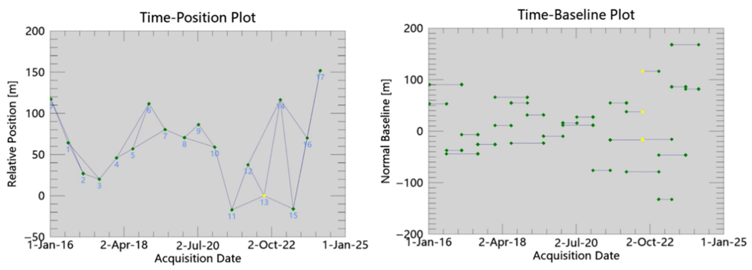
To effectively mitigate the noise component () and address vegetation challenges, a dual-stage coherence filtering strategy was implemented: initially applying a global coherence threshold of 0.35 to ensure phase unwrapping reliability, followed by a refined mean temporal coherence threshold of 0.25 to maximize spatial sampling within landslide bodies [36]. Building on this, the interferometric network incorporates all 118 Sentinel-1A scenes, where the Singular Value Decomposition (SVD) algorithm was employed to jointly invert phase information. Crucially, to explicitly calibrate the systematic orbital and atmospheric errors ( and ), the unwrapped phases were constrained using displacement data from three stable GNSS benchmarks. This calibration strategy effectively aligned the InSAR baseline with the geodetic reference, yielding a high correlation (R2 > 0.90) and a Root Mean Square Error (RMSE) of 4.2 mm between the SBAS-InSAR and GNSS time series. This quantitative consistency confirms the reliability of the retrieved deformation field, demonstrating that residual phase errors were effectively suppressed.
As shown in Figure 3, the final interferometric network incorporates all 118 Sentinel-1A scenes. Although the strict temporal baseline limit reduced redundancy in certain intervals, this configuration effectively excluded low-quality pairs affected by vegetation decorrelation. Crucially, the network remains fully connected, allowing the Singular Value Decomposition (SVD) to jointly invert the phase information. This approach minimizes error propagation through global optimization, ensuring reliable time-series retrieval for all 118 epochs without relying on excessive interferogram redundancy.
2.2.2. Multi-Source Data Preprocessing and Dataset Construction
Following the extraction of the 91 representative monitoring points, the generated raw displacement sequences underwent a standardized preprocessing pipeline. To effectively mitigate high-frequency atmospheric artifacts and stochastic noise while preserving kinematic trends, a 3-point moving-average filter was applied (Equation (3)).
where dt denotes the smoothed displacement at time t, dt−1, dt, and dt+1 represent the original SBAS-InSAR cumulative displacement at time steps t − 1, t, and t + 1, respectively.
While this linear smoothing enhances the signal-to-noise ratio, ensuring it does not over-smooth critical non-linear deformation features is crucial. To address this, Empirical Mode Decomposition (EMD) was employed as a complementary non-linear spectral analysis tool. EMD decomposed the complex displacement time series into Intrinsic Mode Functions (IMFs) to characterize the multi-scale temporal structure of the deformation. This decomposition validated that the high-frequency components suppressed by the 3-point moving average corresponded primarily to noise (comparable to the first IMF), whereas the critical non-linear trends essential for the deep-learning model were preserved. This hybrid approach, combining linear filtering with non-linear spectral validation, ensures the integrity of the landslide kinematic data.
To capture the complex triggering mechanisms of landslide deformation, each sample is represented by a 10-dimensional feature vector. This vector integrates dynamic triggering factors (including SBAS-InSAR cumulative displacement, synchronized NDVI, and daily cumulative precipitation) alongside static geomorphic constraints (slope, aspect, curvature, roughness, geomorphic unit, lithology, and land use). Crucially, the NDVI time series underwent atmospheric correction (FLAASH) and cloud masking (CFMask). To achieve strict spatiotemporal alignment with the 118 Sentinel-1A acquisition dates, NDVI records were temporally resampled using a cubic spline function F(t) (Equations (4) and (5)).
where tSAR denotes the SAR acquisition dates, and F(t) is the piecewise cubic polynomial constructed from the available Landsat NDVI observations NDVIL at times tk, ensuring second-order continuity (C2) across the time series. Spatially, the data were resampled to the same 30 m resolution via bilinear interpolation.
To construct a unified feature vector for the deep-learning model, multi-source variables were concatenated at each time step. To facilitate model convergence and eliminate dimensional heterogeneity, Z-score normalization was applied to all continuous features as shown in Equation (6).
where x denotes the original feature value, z is the standardized (z-score normalized) value, and μ and σ are the mean and standard deviation computed exclusively from the training set. These parameters were subsequently applied to the validation and test sets, strictly preventing statistical leakage from the test set (future data) and ensuring a realistic evaluation of the model’s generalization capability.
Although the number of spatially independent landslide objects is limited to 91, the effective dataset for model training was significantly expanded using a sliding window strategy (window length = 12, step = 1), resulting in a total of 9737 sequences. It is acknowledged that these augmented sequences exhibit temporal dependence due to the overlapping windows. Therefore, to strictly prevent data leakage, a chronological partitioning strategy is employed that ensures zero temporal overlap between the training and testing phases. This guarantees that the model learns complex temporal evolution patterns without exploiting the dependencies between overlapping sequences for prediction.
2.3. Integration of Environmental Variables
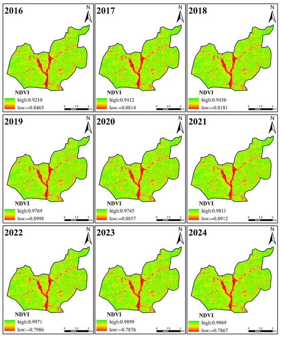
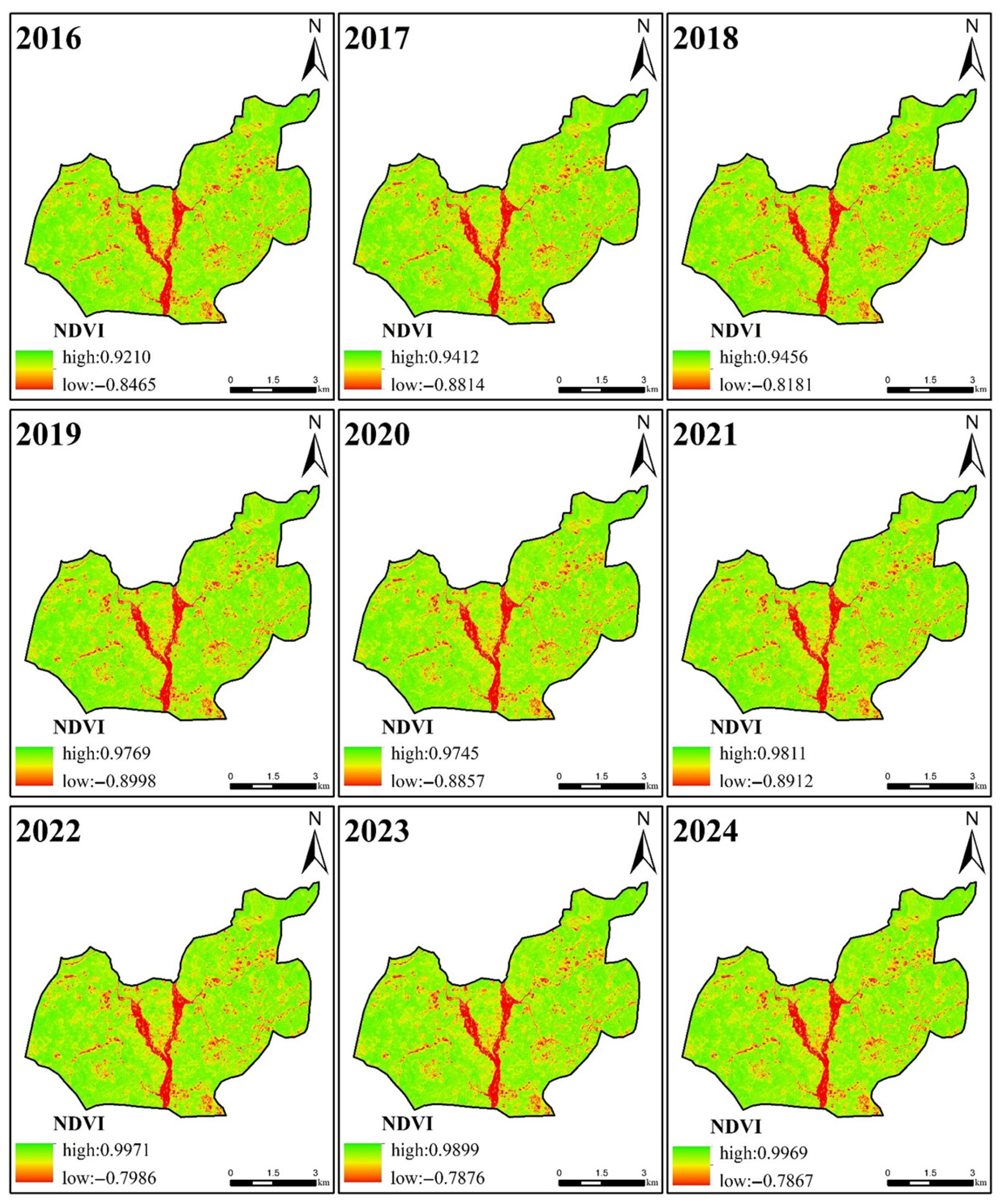
To account for external factors influencing slope stability, multi-source environmental data were incorporated into the prediction framework [37]. The Normalized Difference Vegetation Index (NDVI) was extracted from multi-temporal images corresponding to the SBAS-InSAR observation periods. After atmospheric correction and resampling to match the SAR resolution, NDVI time series were utilized to represent vegetation coverage dynamics and potential anthropogenic disturbances (Figure 4). Areas showing persistent NDVI decline were identified as proxies for deforestation or surface modification, offering auxiliary information for interpreting deformation mechanisms.
Figure 4.
Normalized difference vegetation index (NDVI) analysis.
To construct the multi-dimensional feature vector, static topographic factors (slope, aspect) were integrated alongside the vegetation metrics. Given the inconsistency in spatial resolutions (30 m DEM vs. InSAR pixels), all static factors were resampled using bilinear interpolation. Additionally, land-use classification data, derived from satellite imagery via the Support Vector Machine (SVM) algorithm, were included to quantify human-induced changes [38].
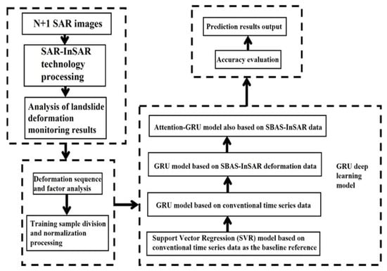
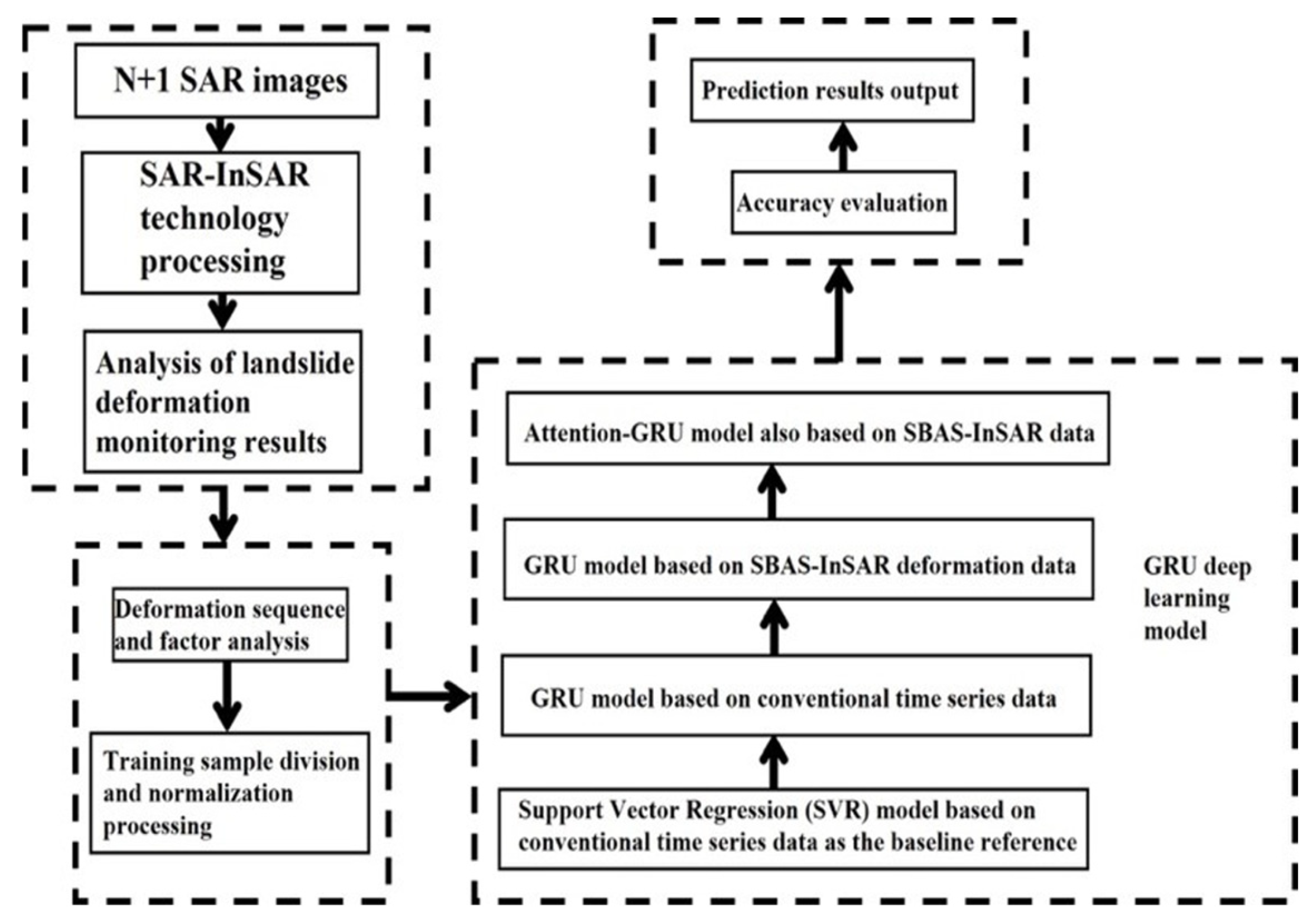
Regarding meteorological factors, it is important to clarify that while rainfall patterns were analyzed to support the qualitative interpretation of deformation trends (e.g., seasonal responses), precipitation data were excluded from the predictive input matrix in this specific implementation. This exclusion allows the assessment to focus strictly on the coupling between geodetic displacement and eco-geomorphic changes. Finally, all selected features underwent Z-score normalization to accelerate the convergence of the deep-learning model, forming the final input tensor for the Attention-GRU method (Figure 5).
Figure 5.
Overview of the experimental workflow, illustrating the parallel application of the baseline SVR model and the proposed Attention-GRU framework to SBAS-InSAR-derived displacement time series and auxiliary environmental data.
2.4. Deformation Zone Identification and Dataset Partitioning
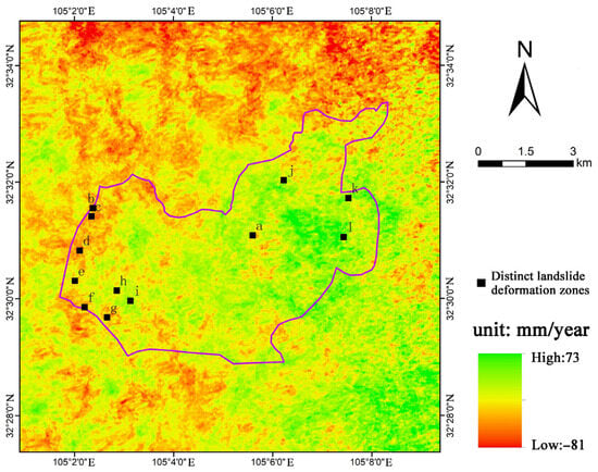
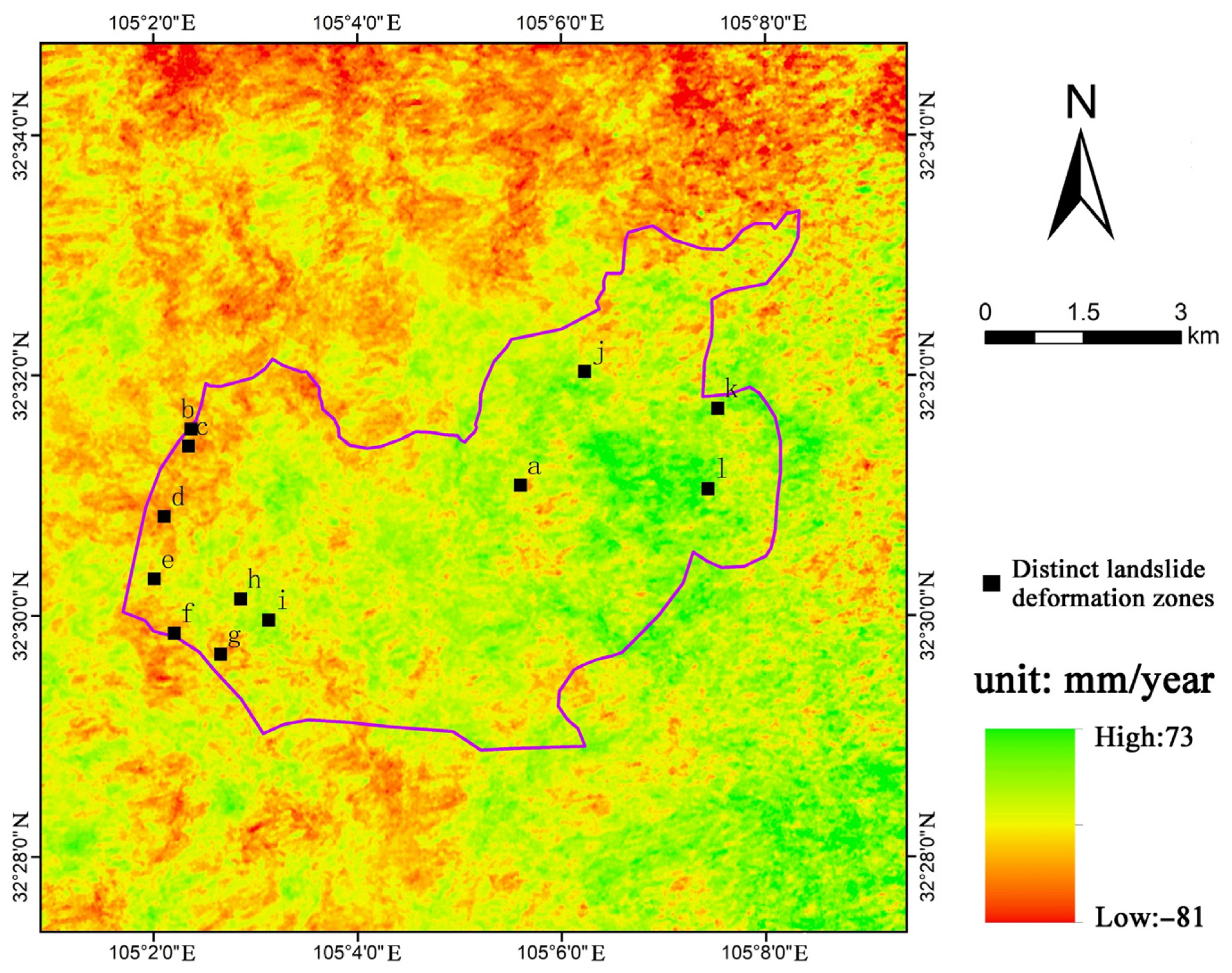
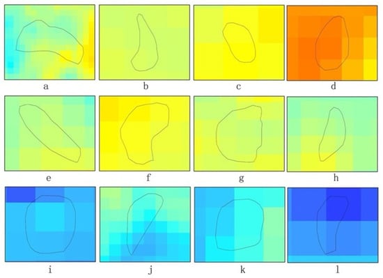
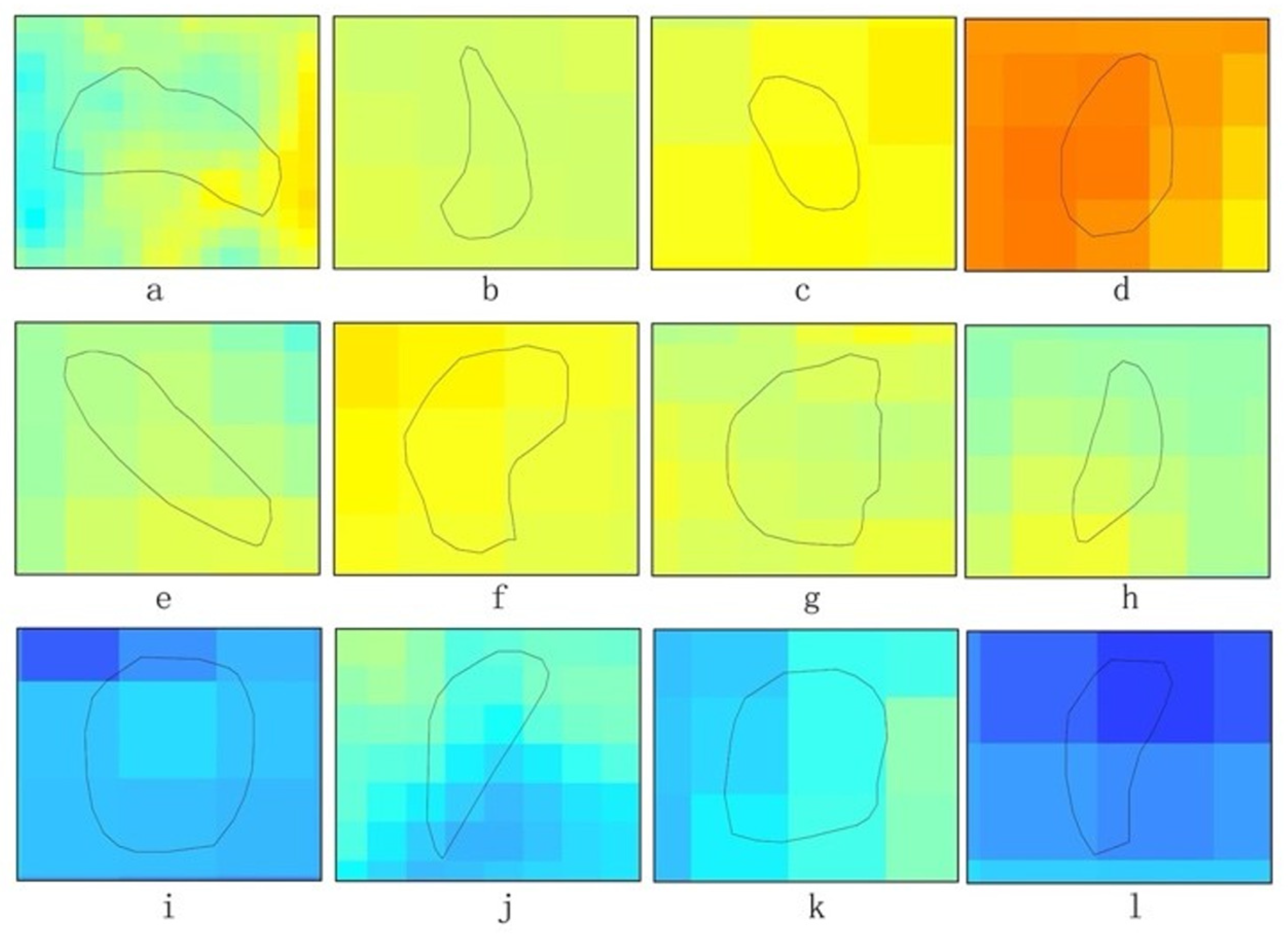
Based on the derived time-series deformation fields, the spatial distribution of surface displacement was analyzed to identify critical instability areas. As illustrated in the Sentinel-1A ascending velocity map (Figure 6), twelve major deformation zones (a–l) were initially delineated as macro-scale spatial units, spanning diverse geomorphic settings including valleys and steep slopes. From within these zones, 91 representative deformation points exhibiting high spatiotemporal consistency were extracted. These points serve as the primary independent spatial units, capturing complex kinematic phases ranging from monotonic creep to accelerated instability (Figure 7).
Figure 6.
Sentinel-1A ascending orbit variable speed diagram.
Figure 7.
Landslide deformation patterns (a–l).
Regarding the distinct “blurred red patterns” observed in the velocity map, careful inspection confirms these correspond to active landslide masses rather than atmospheric artifacts. While stratified atmospheric delays can introduce elevation-dependent signals in individual interferograms, the velocity map represents the mean deformation rate derived via linear regression over the entire multi-year time series. This temporal stacking process effectively suppresses non-systematic atmospheric fluctuations, including seasonal stratified delays that do not exhibit a linear trend. Furthermore, the spatial distribution of these high-deformation zones correlates strictly with unstable topographic features (e.g., steep slopes and valley incisions) rather than showing a pervasive correlation with elevation. Consequently, the influence of residual atmospheric effects on the estimated deformation rates is considered negligible.
Given that the sliding window technique augmented the dataset to 9737 sequences, the inherent issue of temporal dependence was explicitly addressed through a rigorous partitioning strategy. To strictly simulate real-world early warning scenarios, a Chronological Forward Chaining strategy was implemented. The dataset was sequentially divided into training (70%), validation (15%), and testing (15%) subsets strictly according to acquisition time.
To mitigate the potential impact of temporal dependence between overlapping sequences that is a strict temporal cut-off between subsets was ensured. This means that although overlapping windows exist within the training set to facilitate the learning of lag effects, no sequence in the training set overlaps with any sequence in the validation or testing sets. This partitioning prevents temporal information leakage and provides an unbiased assessment of the model’s generalization capability for future, unseen time periods, ensuring the operational validity of the proposed early warning framework.
2.5. Attention-GRU: Model Architecture and Interpretability
To effectively capture the temporal heterogeneity of landslide deformation, an Attention-enhanced Gated Recurrent Unit (Attention-GRU) architecture was constructed. This framework couples a recurrent encoding layer with a temporal attention mechanism to internalize the complex nonlinear geomorphic dependencies inherent in multivariate time series.
2.5.1. Input Structure and Attention Mechanism
Given the raw time-series length of 118 Sentinel-1A acquisition dates per sample, a sliding window approach was employed to generate training sequences. The input window length (L) was empirically set to 12 acquisitions, resulting in an input dimensionality of 12 × 10 (time steps × features) per sequence. This duration strikes a critical balance: a window of 12 steps (approx. 144 days, given the 12-day revisit cycle of Sentinel-1) is sufficiently long to delineate sustained acceleration trends yet concise enough to prevent the dilution of short-term precursory signals by irrelevant historical data.
To process these sequences, the framework incorporates a Temporal Attention Mechanism. Unlike conventional RNNs that assign uniform importance across time steps, this module learns adaptive weights for the input sequence X, where X = {x1,x2,…,xt} represents the multivariate input sequence within a sliding window, and xt denotes the input feature vector at time step t. This enables the model to dynamically prioritize critical deformation phases, specifically the onset of acceleration, while suppressing quiescent periods. Crucially, this attention mechanism complements the preprocessing step: while the 3-point filter reduces high-frequency noise, the attention module effectively identifies and amplifies the underlying acceleration trends, preserving the precursory information essential for early warning.
2.5.2. Recurrent Encoding and Optimization
The attention-weighted sequences serve as input to the GRU layer. Through its internal gating structure, the GRU captures long-term dependencies and mitigates the gradient vanishing problem (Equation (7)).
where xt denotes the input feature vector at time step t (processed by the temporal attention module), and ht−1 is the hidden state from the previous step. The final prediction is derived via a fully connected decoding layer (Equation (8)).
Model parameters θ are optimized by minimizing the Mean Squared Error (MSE) loss function using the Adam optimizer (Equation (9)).
where N is the batch size, and yi represents the observed displacement. Dropout regularization is applied to prevent overfitting, and hyperparameters are rigorously tuned based on validation performance.
2.5.3. Physical Interpretability via SHAP
To ensure the physical transparency of the “black-box” deep learning model, the SHapley Additive exPlanations (SHAP) framework was integrated. SHAP quantifies the marginal contribution of each feature to the model output based on cooperative game theory. In this study, SHAP dependence analysis is utilized to identify nonlinear thresholds and interaction effects among environmental factors (e.g., slope, curvature, and vegetation dynamics). Crucially, this integration transforms the attention mechanism from a latent weighting process into an interpretable physical proxy. This coupling ensures that the model’s focus on specific displacement lags is mechanistically aligned with established geomechanical principles, such as slope-gradient-controlled instability and stress concentration on concave terrain, providing geomechanical credibility to the forecasting results.
2.6. Model Evaluation Metrics
To comprehensively assess the prediction accuracy and robustness of the proposed framework, a multi-dimensional evaluation strategy was implemented. Standard statistical metrics, including the Root Mean Squared Error (RMSE), Mean Absolute Error (MAE), Mean Absolute Percentage Error (MAPE), and the Coefficient of Determination (R2), were selected to quantify the deviation between predicted displacement values and observed ground truth. All evaluation metrics were computed exclusively on the independent testing dataset to eliminate bias. These metrics serve as the uniform standard for benchmarking the proposed Attention-GRU model against baseline methods. The mathematical definitions of these key metrics are explicitly formulated in Equations (10)–(13) as follows.
where N is the number of test samples, yi is the observed displacement value, is the predicted value, and is the mean of the observed values.
3. Results
The SBAS-InSAR monitoring campaign was initiated using Sentinel-1A archives dating back to January 2016. While the initial scenes were primarily used to establish a stable reference phase and initialize the cumulative displacement time-series, the comprehensive kinematic analysis presented in this section covers the full evolutionary sequence extending through March 2024.
3.1. Performance Comparison of Different Prediction Models
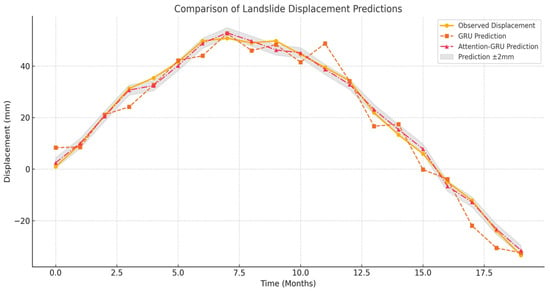
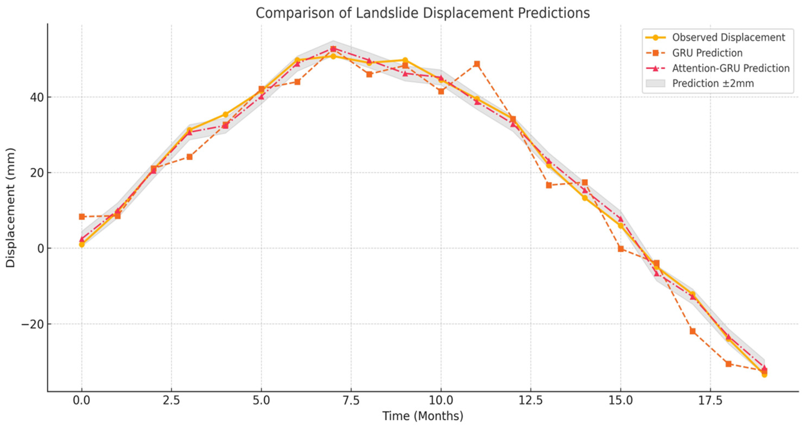
To visually demonstrate the predictive performance of the proposed method, representative monitoring points were selected from the active deformation zones. The specific geographic locations of these sample points (labeled a–l) are clearly marked in the Sentinel-1A velocity map in Figure 6. A comparison of predicted versus observed displacement trajectories for these points is presented in Figure 8. As illustrated, the traditional GRU model (orange dashed line) exhibits noticeable fluctuations, particularly during the peak deformation phase (Months 6–9) and the rapid subsidence phase (Months 15–18), indicating its struggle with nonlinear volatility. In contrast, the Attention-GRU model (red dashed line) aligns closely with the observed data (yellow line), falling almost entirely within the ±2 mm error margin (grey shaded area). This visual evidence confirms that the attention mechanism effectively suppresses noise and captures the trend turning points more accurately than the standard recurrent architecture.
Figure 8.
Comparison of landslide displacement prediction results between GRU and Attention-GRU models. The yellow line represents observed SBAS-InSAR displacement, while the orange and red dashed lines denote predictions from the standard GRU and the proposed Attention-GRU, respectively. The grey shaded region indicates the ±2 mm prediction confidence interval. This figure displays a representative 19-month sequence (a subset of the test set) extracted from the full Sentinel-1A time series (118 scenes).
To further address the model’s sensitivity to acceleration phases, a segment-based error analysis was conducted (Table 3). While both models perform competently during the steady-state period (Months 1–14), the standard GRU’s accuracy diminishes significantly during the critical acceleration phase (Months 15–18). In contrast, the Attention-GRU maintains a low MAPE (approx. 5.2%) and a minimized RMSE (1.08 mm) during this volatile period. This quantitative evidence confirms that the temporal attention mechanism adaptively prioritizes precursory acceleration signals, providing direct evidence of the model’s sensitivity to landslide instability triggers.
Table 3.
Quantitative evaluation of model sensitivity across different deformation phases.
3.1.1. Baseline Experiment: SVR Based on Conventional Data
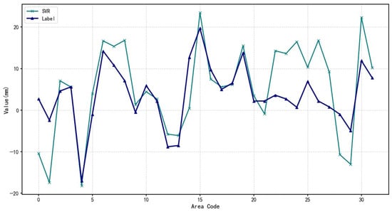
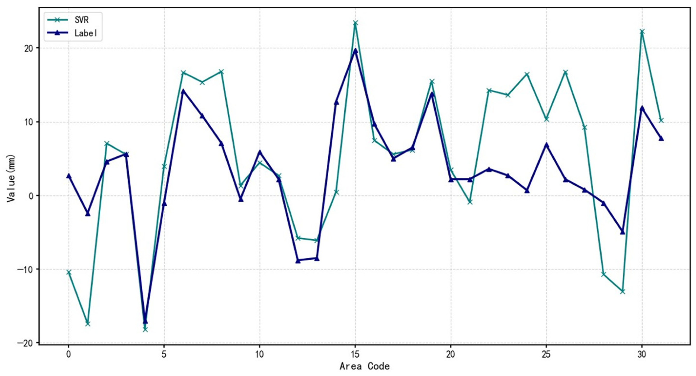
A Support Vector Regression (SVR) model was applied using conventional time series data to establish a baseline (Figure 9).
Figure 9.
SVR model prediction results based on conventional data (Baseline model). The deformation time series shown corresponds to a representative monitoring point selected from the independent test set, extracted from the full SBAS-InSAR time series spanning 2016–2024 (118 Sentinel-1A acquisitions).
As shown in Table 4, SVR struggles with dynamic trend extraction and noise suppression, leading to limited prediction stability. Its high Mean Absolute Percentage Error (MAPE) of 84.372% primarily stems from its inability to handle nonlinear noise effectively in raw time series data.
Table 4.
Performance metrics of SVR model based on conventional data.
3.1.2. Sequential Learning: GRU Based on Conventional Data
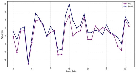
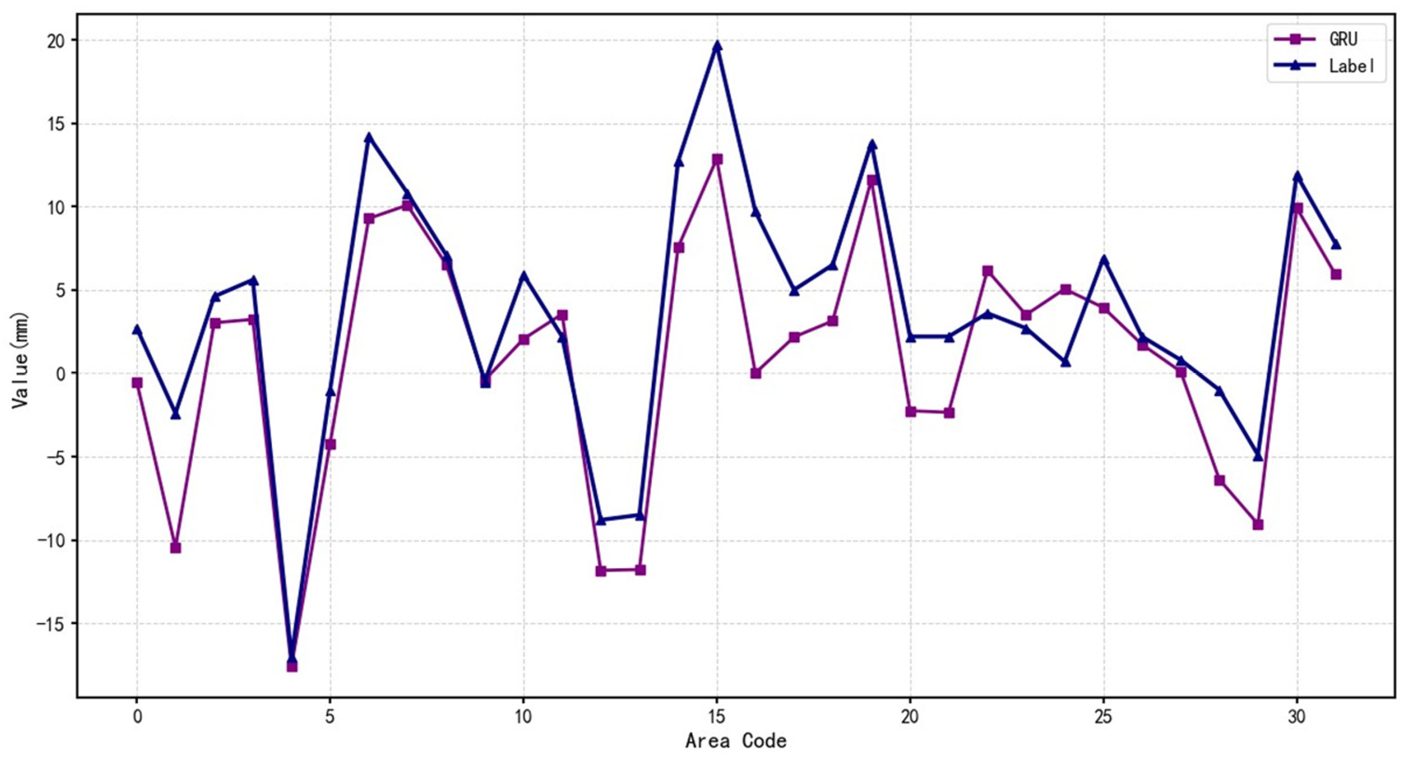
In contrast to SVR, the Gated Recurrent Unit (GRU) model leverages gated mechanisms, specifically the update and reset gates, to capture long-term dependencies while filtering out noise. GRU’s recurrent structure allows it to model abrupt changes and nonlinear acceleration patterns commonly seen in landslide deformation (Figure 10).
Figure 10.
GRU model prediction results based on conventional data. The deformation time series shown corresponds to a representative monitoring point selected from the independent test set, extracted from the full SBAS-InSAR time series spanning 2016–2024 (118 Sentinel-1A acquisitions).
Consequently, the GRU model improved the MAPE to 74.962% (Table 5), demonstrating the advantage of deep learning in time-series modeling.
Table 5.
Performance metrics of the GRU model based on conventional time series data.
3.1.3. Multi-Source Fusion: GRU Based on SBAS-InSAR Data
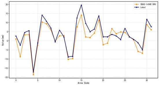
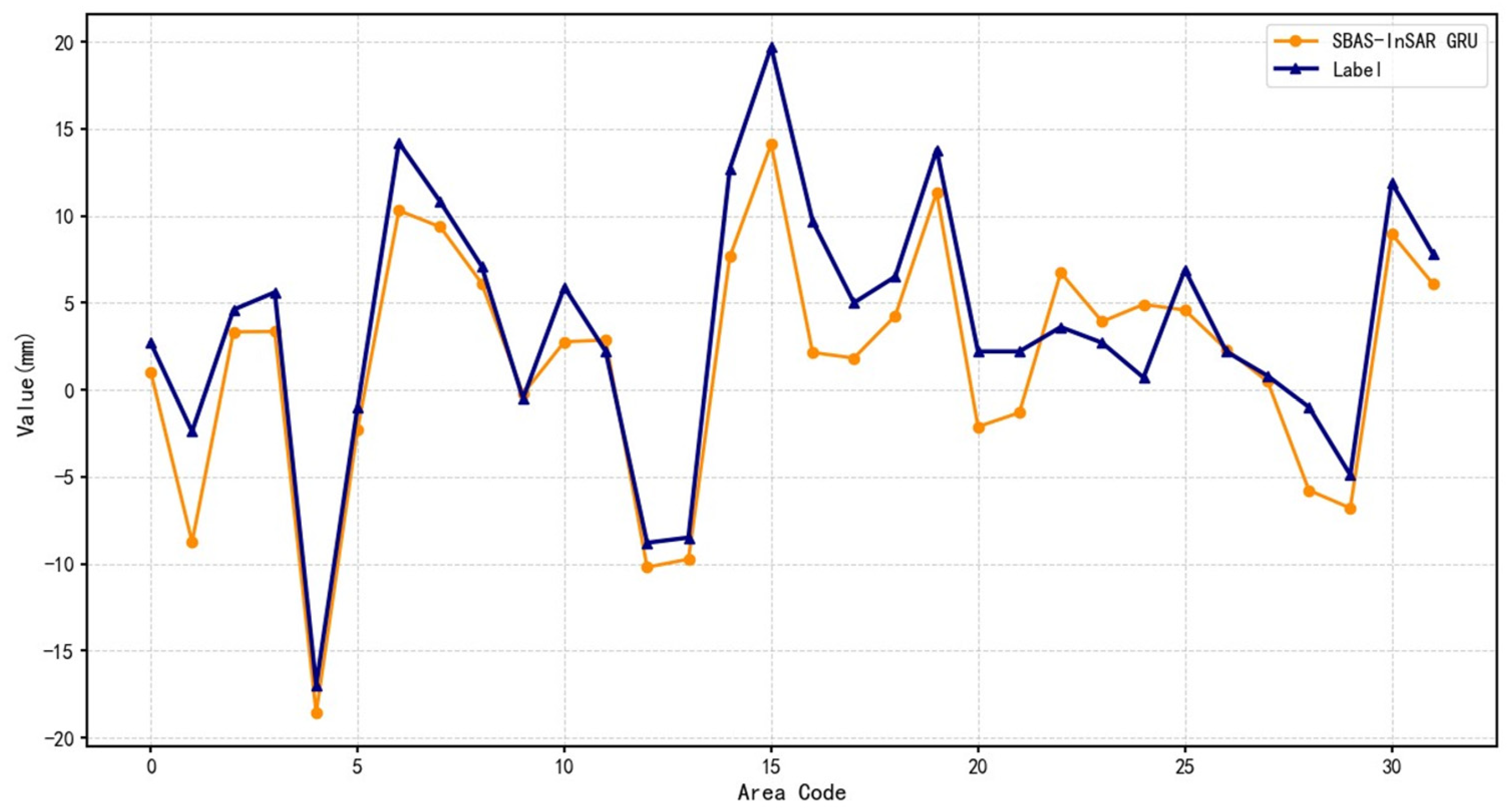
Building upon GRU’s sequential learning capabilities, high-precision SBAS-InSAR data were incorporated to enable multi-source data fusion (Figure 11). The SBAS-InSAR deformation time series were pre-processed via a 3-point sliding average filter and linear trend removal. While this smoothing step effectively suppresses high-frequency atmospheric and decorrelation noise, it inevitably attenuates some short-term fluctuations. To address this, the subsequent attention mechanism is configured to specifically extract physically meaningful, temporally localized acceleration signals.
Figure 11.
GRU model prediction results based on SBAS data. The deformation time series shown corresponds to a representative monitoring point selected from the independent test set, extracted from the full SBAS-InSAR time series spanning 2016–2024 (118 Sentinel-1A acquisitions).
This integration enhances the model’s contextual awareness, reducing the MAPE significantly to 61.498% (Table 6).
Table 6.
Comparison of GRU model performance metrics based on conventional and SBAS data.
3.1.4. Proposed Method: Attention-GRU Based on SBAS-InSAR Data
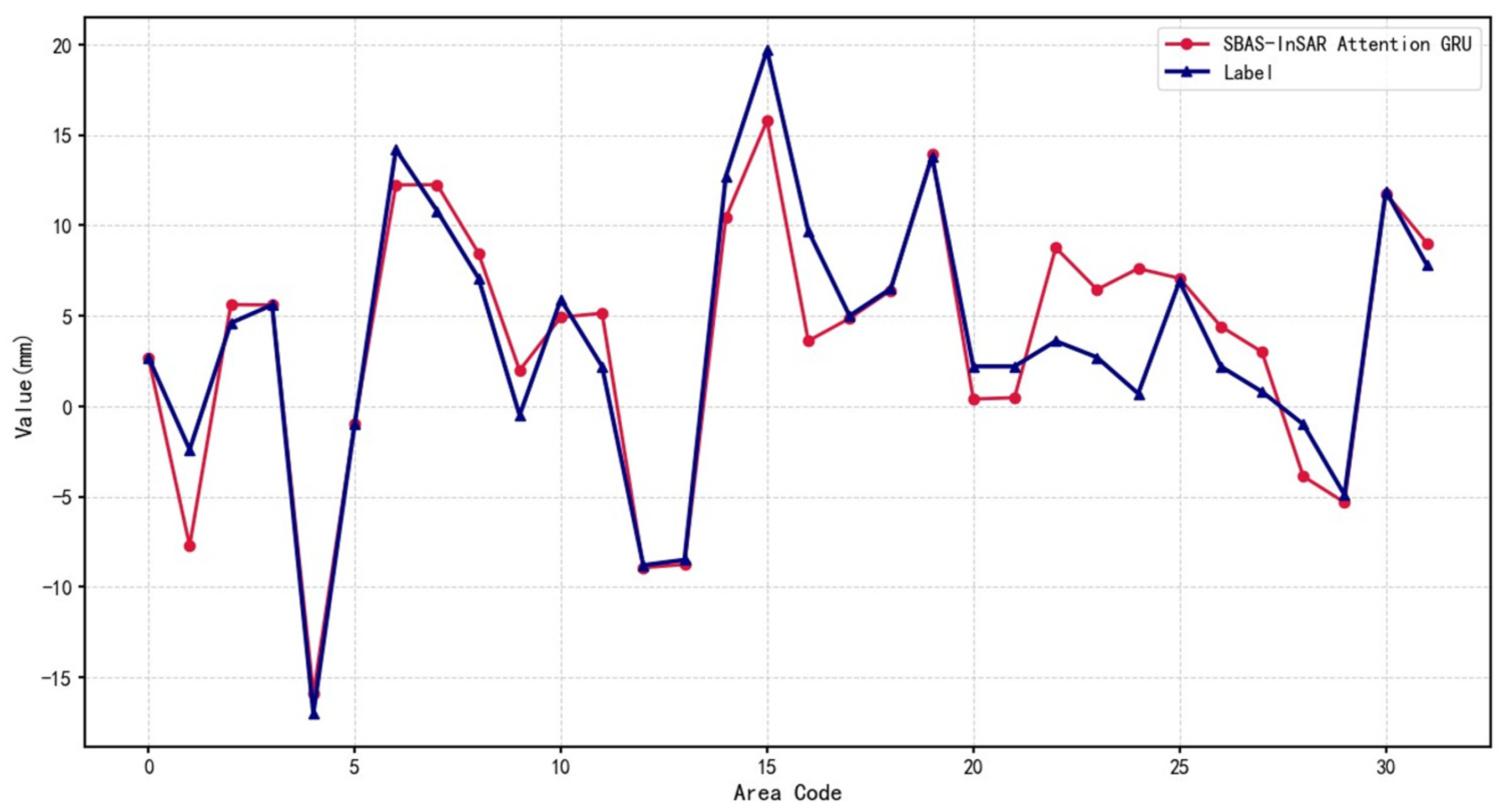
While GRU effectively models temporal trends, its uniform weighting may overlook critical inflection points. The proposed Attention-GRU model introduces an adaptive attention mechanism to dynamically emphasize time steps with higher influence on future outcomes (Figure 12).
Figure 12.
Attention-GRU model prediction results based on SBAS data. The deformation time series shown corresponds to a representative monitoring point selected from the independent test set, extracted from the full SBAS-InSAR time series spanning 2016–2024 (118 Sentinel-1A acquisitions).
Quantitative assessment within the Le’an Town cluster validates the predictive fidelity of the proposed framework, which yields a Mean Absolute Percentage Error (MAPE) of 48.356% and a coefficient of determination (R2) of 0.93 (Table 7). Relative to the traditional SVR baseline, this performance constitutes a 42.7% reduction in MAPE, underscoring the critical advantage of coupling temporal attention mechanisms with multi-stage signal denoising. Crucially, the high R2 value should be interpreted as a reflection of the architecture’s sensitivity to the intrinsic kinematic evolution of landslide units during active deformation phases. Given that the training inputs are derived from localized zones exhibiting pronounced SBAS-InSAR displacement, these metrics signify a robust convergence with the temporal trajectories of identified geomorphological hazards, rather than asserting immediate generalizability for regional-scale spatial extrapolation across predominantly stable terrains.
Table 7.
Performance metrics of Attention-GRU model based on SBAS data.
These metrics reflect the aggregate performance across all 91 validation samples, encompassing phases of both stability and monotonic creep. The elevated MAPE (48.356%) relative to the low RMSE (2.658 mm) results from the prevalence of near-zero displacement values during stable periods. In such low-magnitude contexts, the percentage error calculation becomes highly sensitive, causing minor absolute deviations to manifest as inflated percentage values despite the high precision of the model.
3.1.5. Comparative Analysis of Prediction Accuracy
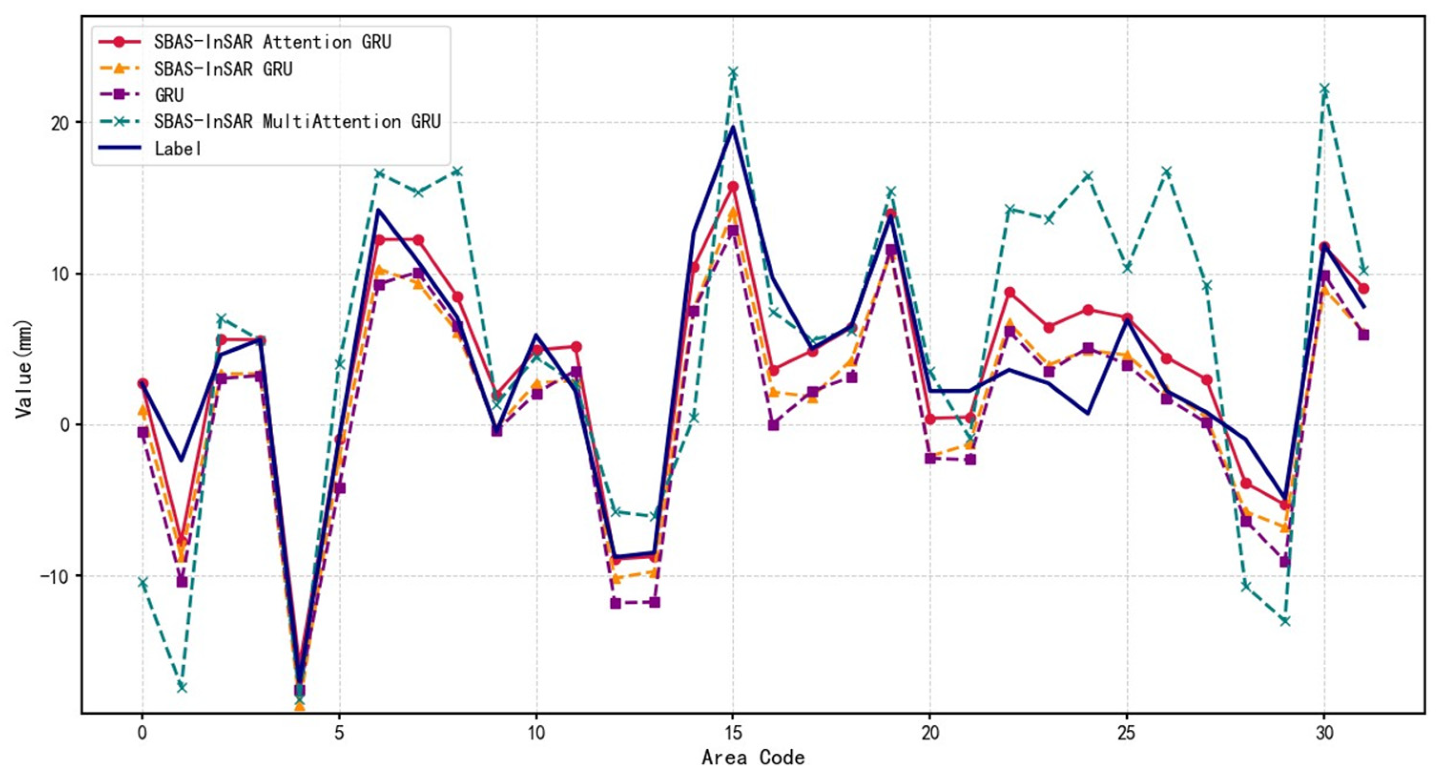
Traditional InSAR technology faces inherent challenges when processing deformation data in landslide-prone areas, as susceptibility to noise interference and data accuracy limitations often leads to biased prediction outcomes. In contrast, the Attention-GRU architecture incorporates an attention mechanism that enables precise capture of critical temporal features and evolutionary characteristics during the landslide process, thereby enhancing displacement prediction capabilities. Comparative analysis of the four experimental results demonstrates that the introduction of the Attention-GRU technique effectively compensates for the deficiencies of conventional InSAR methods, significantly improving prediction accuracy. Specifically, the attention mechanism adaptively assigns varying weights to different time steps within the input data, emphasizing moments with substantial impact on the prediction while attenuating irrelevant or noisy components (Figure 13).
Figure 13.
Comparison of experimental results. The deformation time series shown corresponds to a representative monitoring point selected from the independent test set, extracted from the full SBAS-InSAR time series spanning 2016–2024 (118 Sentinel-1A acquisitions).
3.2. Sensitivity Analysis of Window Length L
To rigorously justify the selection of the input window length L = 12 and evaluate the robustness of the proposed framework, a sensitivity analysis was conducted by varying the temporal receptive field. We tested the Attention-GRU model with L∈{6,9,12,15,18}, representing different historical memory spans. The quantitative comparison is detailed in Table 8.
Table 8.
Performance comparison of the Attention-GRU model under different input window lengths (L).
As shown in Table 8, the Attention-GRU model maintains high predictive capability (R2 ≥ 0.86) across all tested configurations, demonstrating the framework’s strong robustness to hyperparameter variations. Specifically, the predictive accuracy initially improves and then stabilizes as the window length increases.
The optimal performance is achieved at L = 12 (R2 = 0.93, RMSE = 1.42 mm). Physically, this window corresponds to approximately 144 days (given the 12-day revisit cycle of Sentinel-1A), which effectively encompasses the typical duration of seasonal hydrological cycles and the pre-failure acceleration phases of landslides in this region. When L is too short (e.g., L = 6), the model lacks sufficient historical context to differentiate sustained kinematic trends from transient noise, resulting in higher RMSE (2.15 mm). Conversely, extending L beyond 12 (e.g., L = 15,18) introduces marginal returns in accuracy but linearly increases computational cost, likely due to the inclusion of redundant or less relevant distant historical data. Consequently, L = 12 was selected as the optimal configuration that balances predictive precision, physical interpretability, and computational efficiency.
3.3. Interpretability Analysis and Physical Mechanism Verification
While superior performance metrics validate the accuracy of the Attention-GRU framework, they do not inherently explain the underlying decision-making logic. To ensure the model captures physically meaningful geomechanical principles rather than merely overfitting data distributions, SHAP (SHapley Additive exPlanations) is employed to visualize feature contributions and interaction effects.
3.3.1. Global Feature Importance
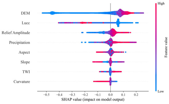
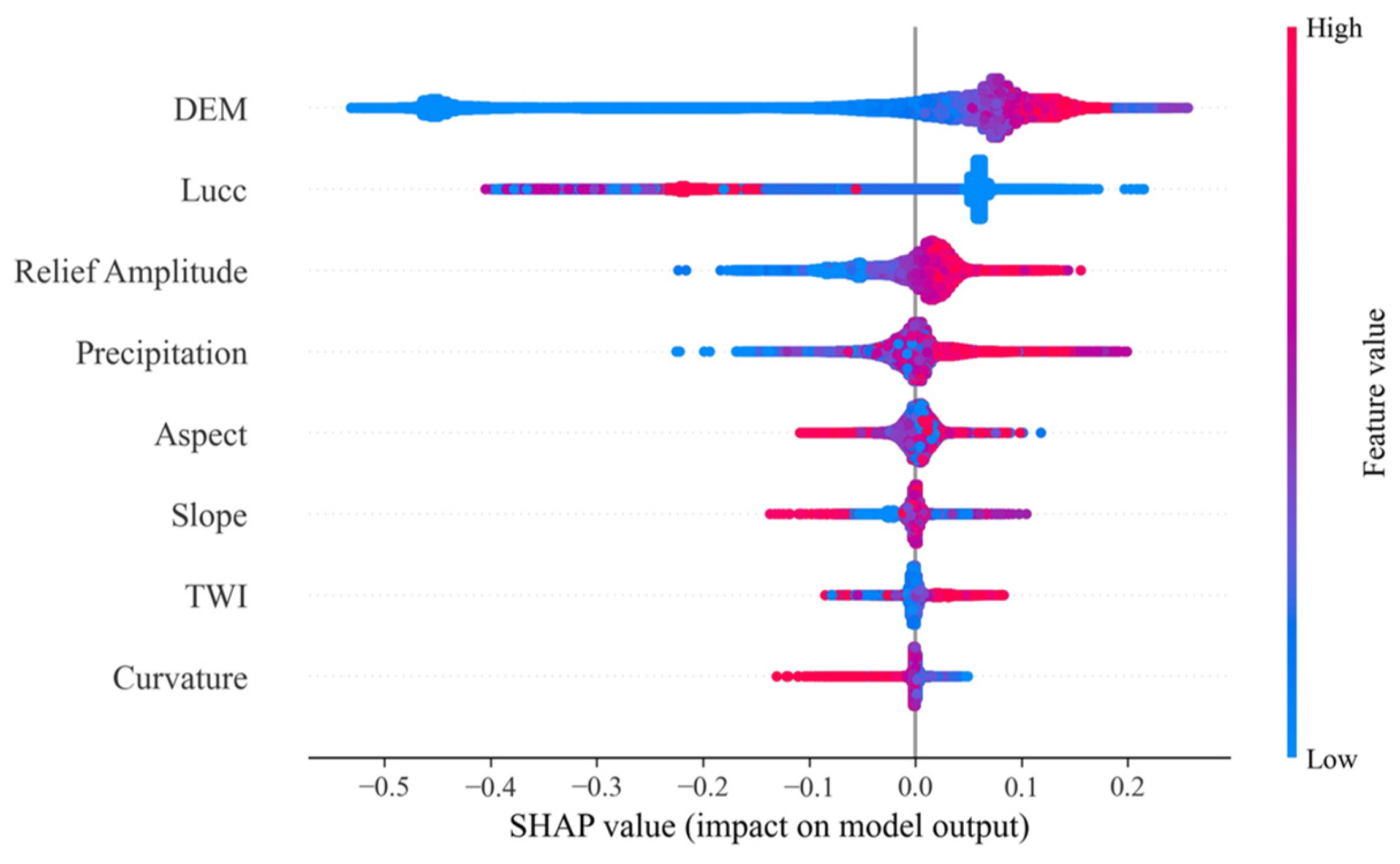
The SHAP summary plot (Figure 14) visualizes the distributional impact of input features on model predictions. The extensive dispersion of SHAP values for DEM indicates that the model exhibits high sensitivity to elevation variations, establishing it as a critical discriminator of deformation risk across the study area. Conversely, the dense clustering observed for variables such as Curvature implies a more constrained contribution to the overall decision boundary.
Figure 14.
SHAP summary beeswarm plot. The plot illustrates the distribution and directional impact of input features on deformation prediction, with wider dispersion indicating higher variance in feature influence.
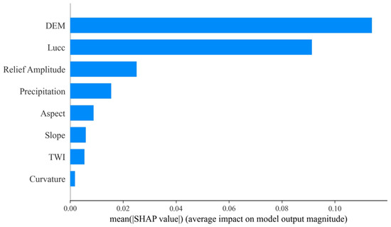
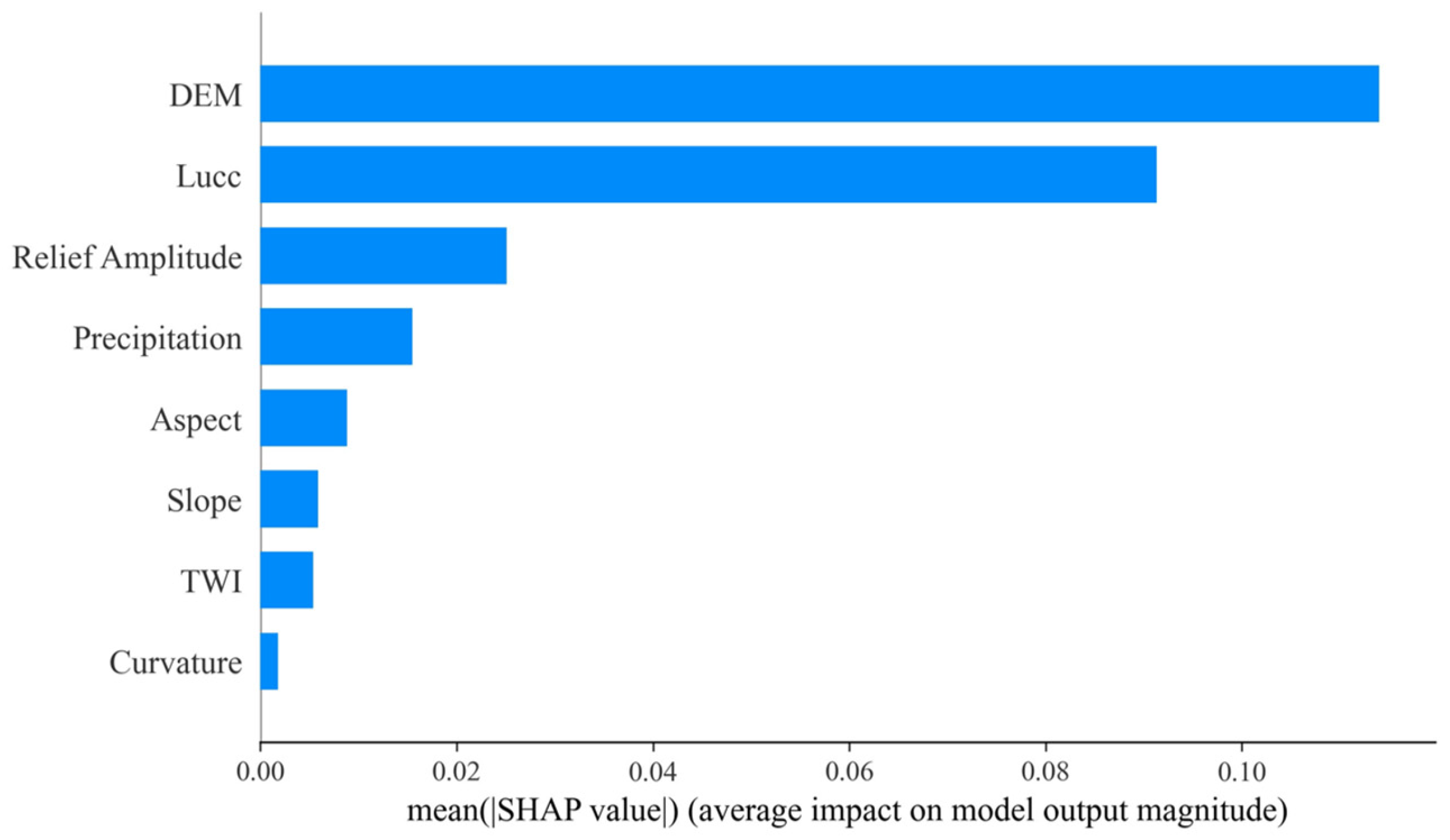
Quantitative analysis via mean absolute SHAP values (Figure 15) further corroborates this feature hierarchy, identifying DEM (Elevation) and Lucc (Land Use/Cover) as the primary determinants of landslide displacement. This statistical ranking is physically consistent with geomechanical principles, where gravitational potential energy and surface material properties govern slope stability mechanics.
Figure 15.
Global feature importance ranking. Features are ranked by mean absolute SHAP values, identifying DEM and Lucc as the dominant drivers of landslide deformation.
3.3.2. Nonlinear Geomechanical Response
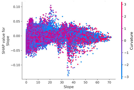
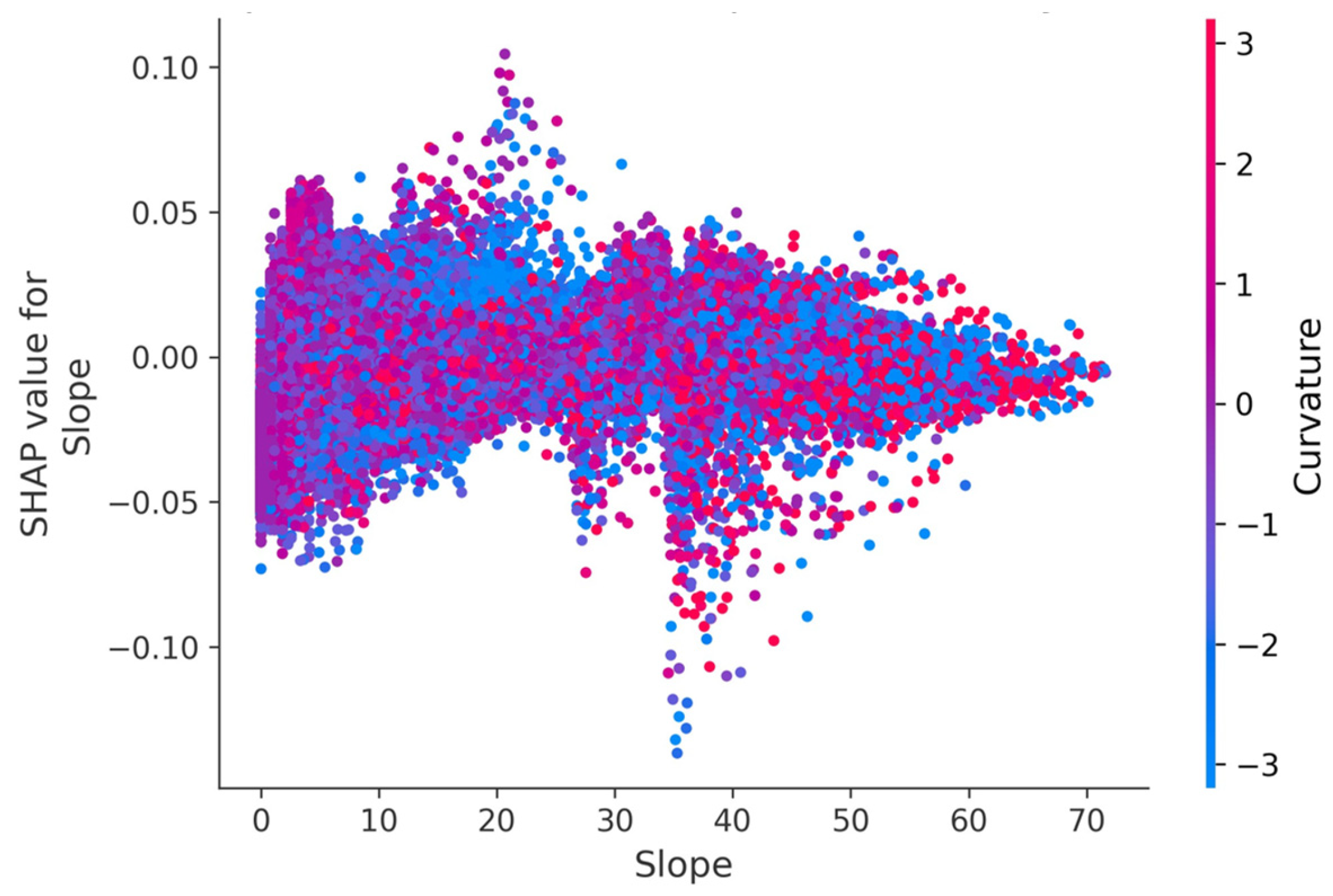
The SHAP dependence plot for Slope (Figure 16) uncovers the model’s ability to resolve complex nonlinear mechanisms governing landslide dynamics. A distinct geomechanical transition is observable around the 35° threshold. In the gentle-to-moderate slope range of 0–35°, SHAP values exhibit dense clustering with significant positive contributions, indicating that these gradients constitute the primary zones for active deformation, likely attributable to the widespread accumulation of loose colluvial deposits. Beyond 35°, a sharp decline in SHAP values is observed, often transitioning to negative values. This pattern suggests a shift in stability mechanisms, where steeper slopes are likely composed of stable bedrock or have already shed unstable material, thus exhibiting a suppression effect on further deformation. Furthermore, the integration of Curvature (represented by the color scale) highlights interaction effects, demonstrating that the model interprets slope stability within the context of micro-topographical stress concentrations rather than as an isolated variable. These findings confirm that the proposed method successfully transforms data-driven forecasting from an opaque regression task into a transparent, physically interpretable diagnostic tool.
Figure 16.
SHAP dependence plot for Slope. The x-axis represents slope angle (°), and the color scale represents Profile Curvature. The plot reveals a non-linear geomechanical response with a distinct stability transition threshold around 35°.
3.4. Spatial Distribution of Landslide Deformation in Le’an Town
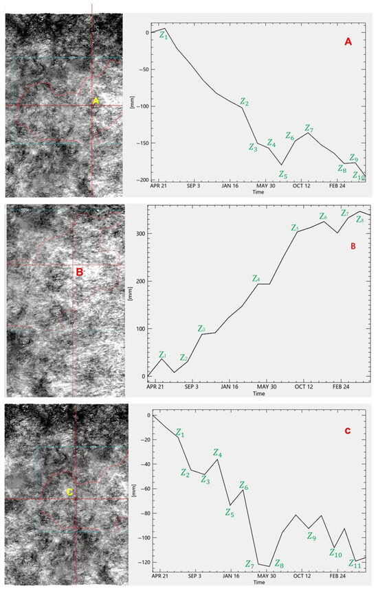
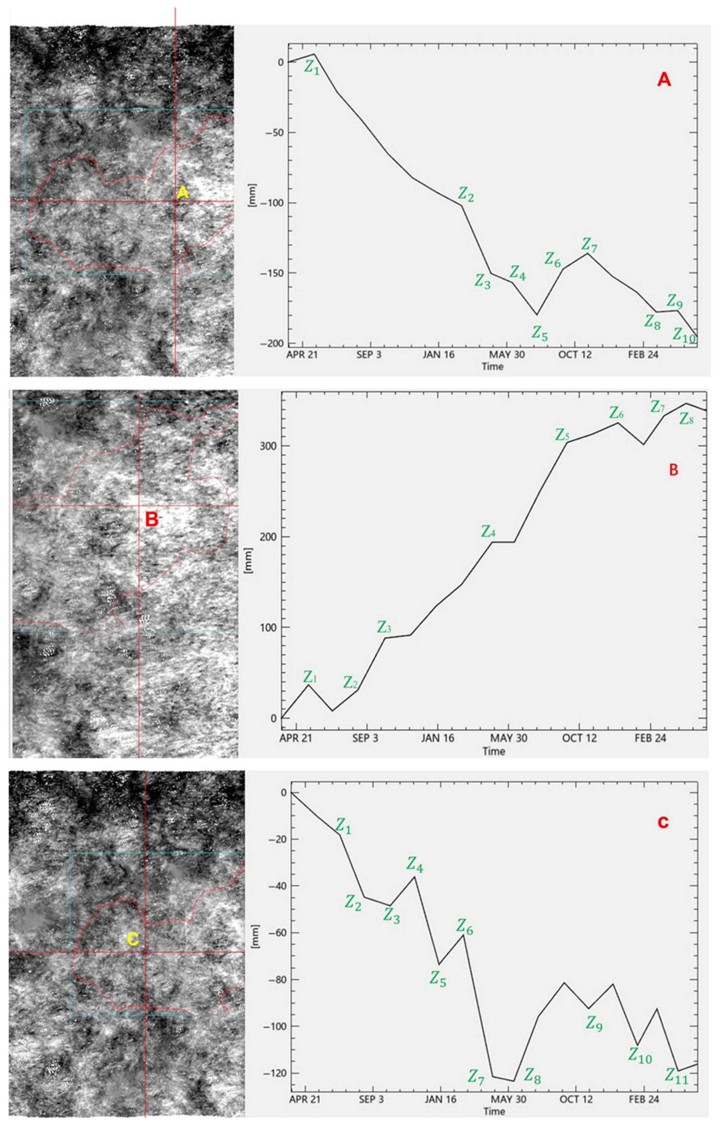
SBAS-InSAR interferometric analysis performed on Sentinel-1A data from January 2016 to March 2024 generated average deformation velocity maps, identifying three distinct areas of displacement: Region A (Central), Region B (Northeastern), and Region C (Southwestern) (Figure 17).
Figure 17.
Distribution of the most prominent landslide displacement settlement areas in the study region (Region (A): Central, Region (B): Northeastern, Region (C): Southwestern). The figure illustrates spatial patterns of cumulative deformation derived from SBAS-InSAR analysis and is used to identify representative deformation zones for subsequent temporal analysis, rather than to evaluate classification performance.
Region A exhibited significant subsidence, with accumulated settlement reaching −100 mm (Z2) from May 2022 to March 2023, and a maximum settlement of −194 mm in November 2023 (Z10). Conversely, Region B showed an overall uplift trend, characterized by a deformation magnitude of 190 mm between July 2022 and April 2023, followed by a significant uplift of 300 mm through September 2023. Region C displayed a moderate settlement trend compared to Region A, with a maximum settlement of −120 mm (Z7) recorded in April 2023. High-resolution image recognition further revealed varying degrees of deformation, including subsidence along the slip direction and uplift at the landslide forefront, confirming the spatial heterogeneity of the landslide cluster.
3.5. Relationship Between NDVI Variation and Surface Deformation
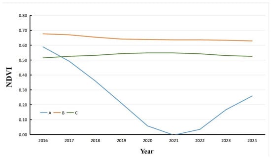
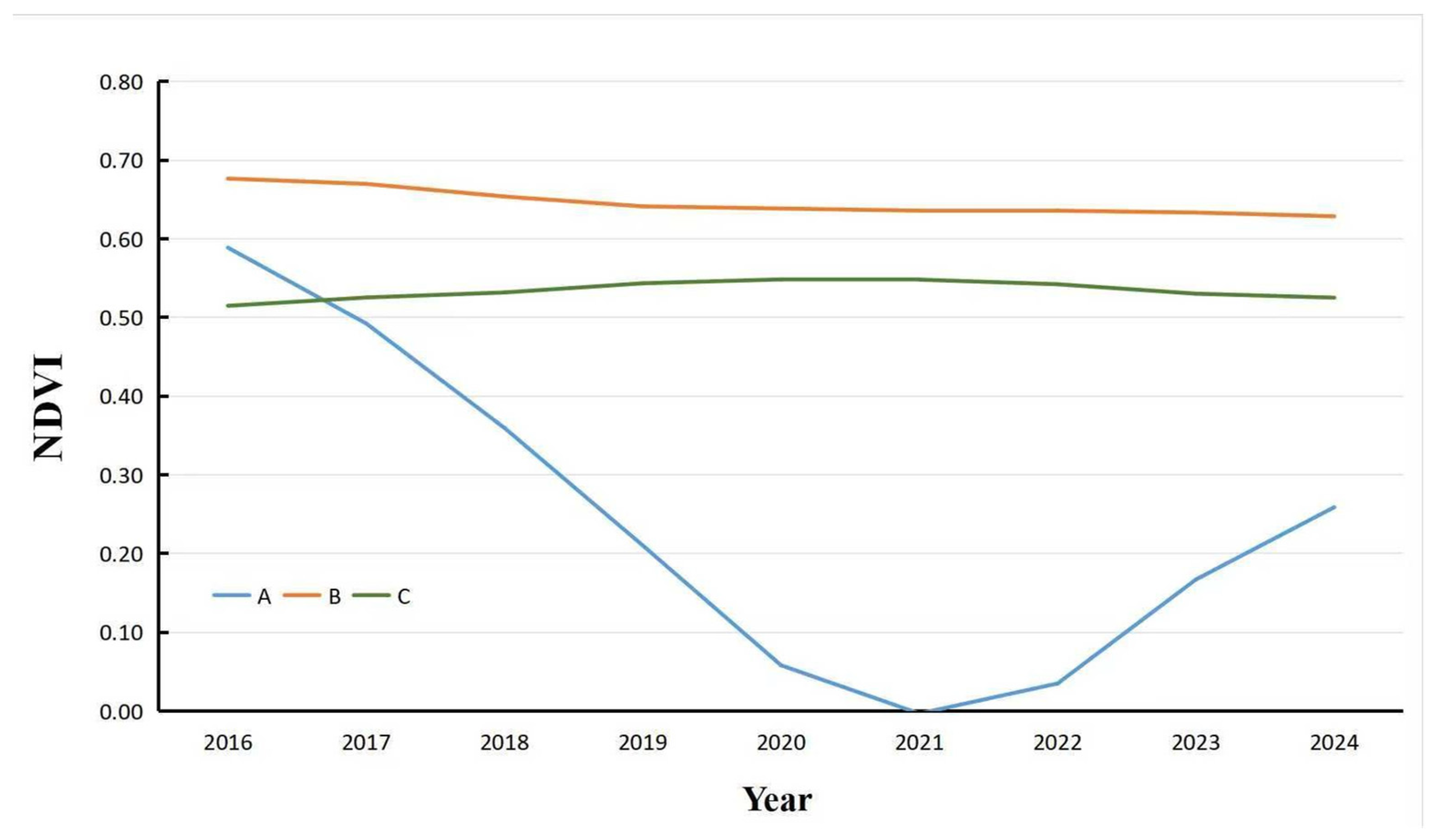
Representative temporal profiles of interannual NDVI variations were extracted for the identified deformation zones (Figure 18) to investigate the hypothesized deformation–ecology feedback. Visual inspection suggests that vegetation coverage trends are synchronized with surface stability evolution. Specifically, Region A exhibits a consistent NDVI decline post-2016, consistent with continuous landslide-induced subsidence. Region B displays a trend reversal, where an initial NDVI increase is followed by a decline after 2021, coincident with accelerated deformation detected by InSAR. Similarly, Region C shows a monotonic decrease in NDVI after 2018, paralleling the observed moderate subsidence.
Figure 18.
Interannual variation of NDVI (Normalized Difference Vegetation Index) line chart.
To substantiate these qualitative observations and rigorously verify the physical coupling, a Pearson correlation analysis was performed between the NDVI time series and the corresponding absolute displacement rates. Additionally, a spatial coincidence test was conducted to quantify the geographical overlap between deformation hotspots and vegetation degradation clusters (Table 9).
Table 9.
Quantitative evaluation of the coupling between NDVI dynamics and displacement intensity (Spatial coincidence is defined as the percentage of high-displacement pixels falling within a 50 m buffer of significant NDVI decline zones).
Statistical analysis reveals a significant negative correlation (mean r = −0.663, p < 0.05), quantitatively confirming that vegetation degradation intensifies as surface displacement rates increase. The spatial coincidence test further corroborates this association, showing that 83.0% of identified high-displacement zones geographically overlap with areas of significant NDVI decline. This quantitative evidence supports the existence of a physical feedback mechanism between surface deformation and ecological response. Consequently, the model’s reliance on NDVI features is grounded in verified physical coupling, indicating that the predictive capability stems from interpretable geo-environmental interactions rather than unexplainable “black-box” correlations.
3.6. Selection of Characteristic Monitoring Points
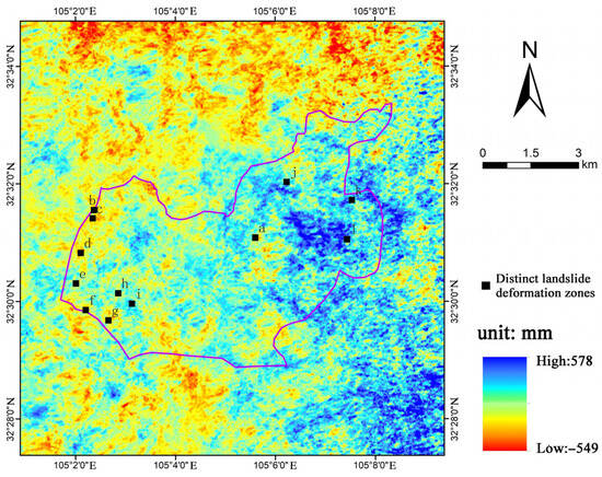
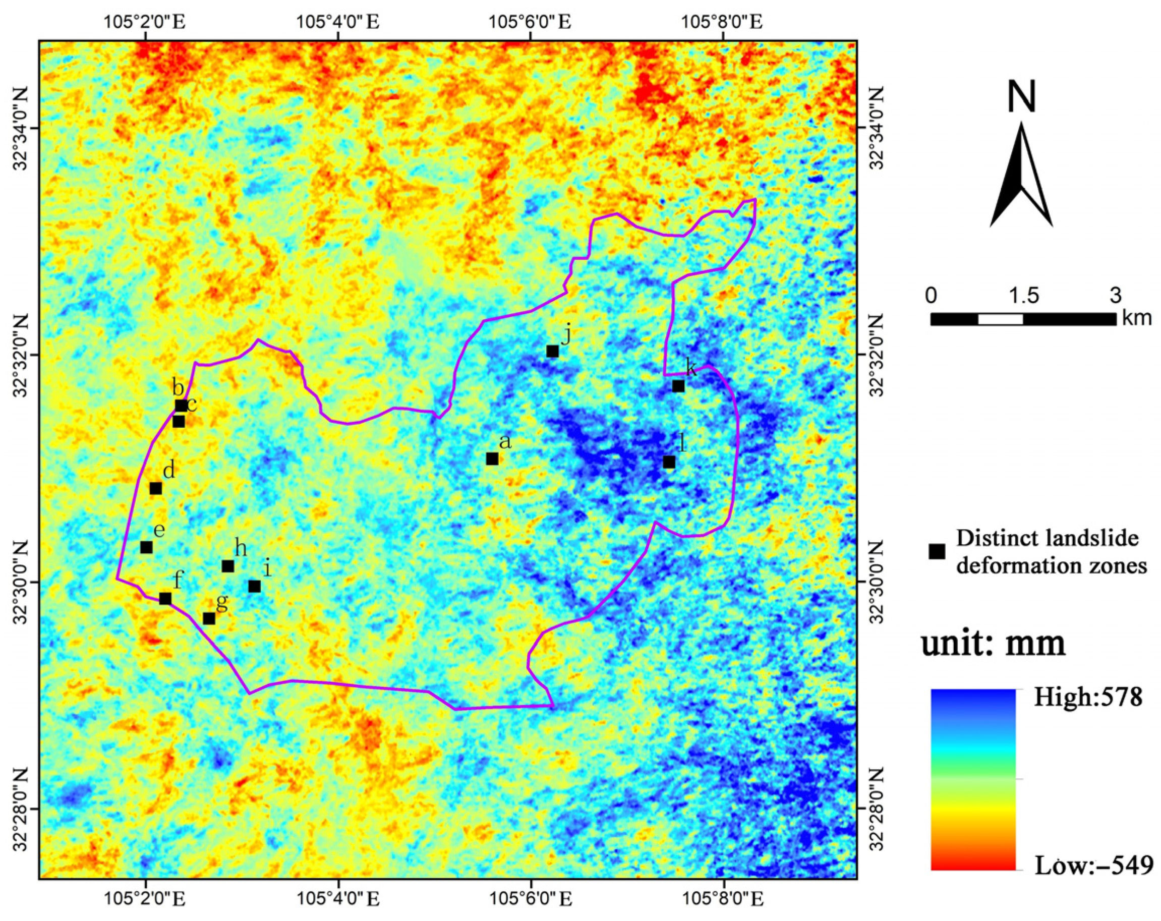
To systematically investigate the fine-scale evolution mechanism of the landslide, twelve representative monitoring points (labeled a–l) were identified based on the cumulative deformation characteristics derived from the SBAS-InSAR time series (Figure 19). This spatial discretization reveals significant heterogeneity in deformation magnitude across the landslide body, with cumulative values ranging from −549 mm to 578 mm. The selected points are strategically distributed to capture distinct deformation behaviors: points in the western sector (e.g., b, c, d) and the southern boundary (f, g) exhibit different deformation intensities compared to the central and eastern regions (a, j, k). The identification of these key locations provides a critical spatial basis for the subsequent extraction of nonlinear temporal evolution patterns and stability assessment.
Figure 19.
Spatial distribution of cumulative deformation and locations of twelve representative monitoring points (a–l) selected for distinct deformation zone analysis.
3.7. Model Validation and Performance Evaluation
The predictive outcomes demonstrate that the Attention-GRU framework maintains robust reliability even under stringent testing constraints. As detailed in Table 10, the test set yielded an aggregate coefficient of determination (R2) of 0.93 and a Root Mean Square Error (RMSE) of 9.348 mm. These high-precision results confirm that the model successfully captures generalized geomechanical evolution laws, validated through the rigorous dual-constraint spatiotemporal partitioning strategy. However, a distinction regarding the metric definitions is necessary for proper interpretation. The low Mean Absolute Percentage Error (MAPE) of 0.51% results from computing errors against the total cumulative displacement over the entire monitoring period. Given the large magnitude of cumulative deformation, the relative percentage error is inherently minimized. Conversely, the MAPE values are derived from step-wise incremental displacement, which is more sensitive to short-term fluctuations and consequently yields higher error percentages. These two schemes are complementary: cumulative metrics quantify long-term trend fidelity, while incremental metrics assess the model’s responsiveness to instantaneous acceleration.
Table 10.
Performance evaluation indices for the landslide prediction model on the independent testing set.
This evaluation focuses specifically on independent test sequences exhibiting significant cumulative displacement and acceleration trends. The observed increase in RMSE (to 9.348 mm) physically corresponds to the larger magnitude of movement in these active deformation zones. Conversely, the MAPE decreases to 0.51% because the substantial cumulative displacement functions as a larger denominator, minimizing the relative error and indicating high predictive fidelity during critical instability phases.
Based on the twelve representative monitoring points (a–l) identified in the previous spatial analysis, their designation as independent spatial testing units further reveals the framework’s adaptability across distinct kinematic regimes (Table 11).
Table 11.
Predictive performance of the Attention-GRU model on two representative landslide samples.
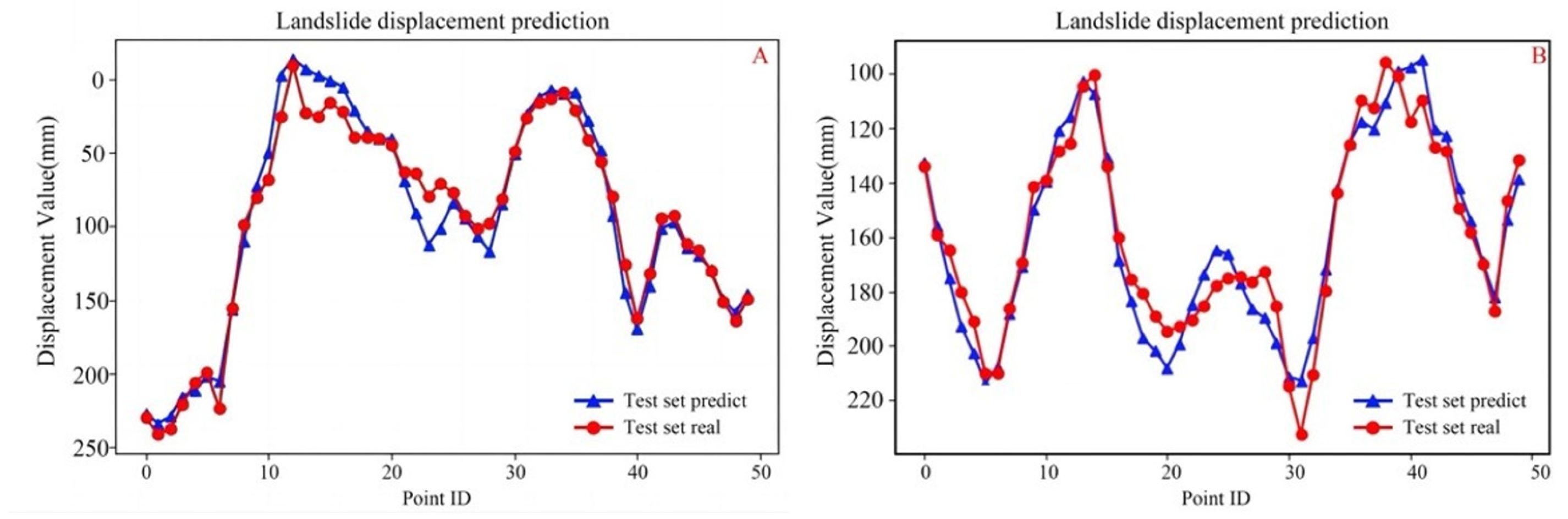
Sample 1 is situated within the central active zone, sharing kinematic characteristics with points a and d which exhibit intense high-frequency seasonal oscillations. In this sector, the model maintained a high correlation of 0.96; however, the stochastic nature of rainfall-induced responses resulted in a localized RMSE of 13.38 mm. Conversely, Sample 2 represents the rear zone characterized by steady deformation trends (analogous to points j and l). Although this area exhibits larger cumulative deformation magnitudes, its motion follows a more consistent monotonic trend. This consistency allowed the model to achieve superior stability with an RMSE of 9.35 mm and a Mean Absolute Percentage Error (MAPE) of only 5.10%.
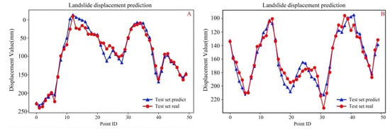
The displacement trajectories for these validation sites are visualized in Figure 20. The predicted values (blue triangles) closely track the observed SBAS-InSAR ground truth (red dots) throughout the test sequence. These observations confirm that despite the strict physical decoupling of temporal and spatial data, the model maintains high predictive consistency across diverse deformation sectors (a–l). Such cross-sector generalization capability demonstrates that the Attention-GRU architecture effectively resolves complex deformation modes, thereby satisfying the reliability requirements essential for operational landslide early-warning systems.
Figure 20.
Comparison of predicted (blue) and observed (red) displacement on the test set for two representative samples. (A) Sample 1: Central Active Zone; (B) Sample 2: Rear Stable Zone.
4. Discussion
This study establishes a physically interpretable landslide displacement forecasting framework by coupling SBAS-InSAR time series with a temporally adaptive Attention-GRU model. Quantitative evaluation in the seismically active Longmen Mountain Fault Zone confirms that the proposed method significantly outperforms conventional baselines, achieving a coefficient of determination (R2) of 0.93 and reducing the Mean Absolute Percentage Error (MAPE) by 42.7% compared to Support Vector Regression. However, it is essential to critically contextualize these high performances metrics. The reported accuracy represents location-specific predictive capabilities strictly within identified active landslide zones. The high R2 value reflects the model’s proficiency in capturing the internal temporal kinematics of slopes that are already exhibiting deformation signals, rather than suggesting a capacity for regional-scale spatial generalization across unseen stable terrains. Nevertheless, the value of this study extends beyond incremental accuracy improvements within these specific zones. Its primary contribution lies in three methodological innovations regarding temporal mechanism modeling, validation rigor, and physical interpretability.
The adaptive temporal attention mechanism effectively internalizes the underlying mechanical evolution of post-seismic slopes. The predictive alignment observed suggests that the model does not merely fit statistical noise but isolates critical kinematic shifts. This behavior mirrors recent investigations into creep failure mechanics [39,40], where the onset of acceleration signifies a critical transition in damage states. While other recent deep learning applications primarily focus on data imputation or inversion tasks [41,42], our analysis reveals that the attention module specifically captures physically meaningful precursory acceleration as sustained multi-epoch trends. This confirms that the model autonomously distinguishes between background noise and the non-linear velocity increments characteristic of genuine instability.
A strict landslide-object-based data partitioning strategy was implemented to explicitly eliminate spatiotemporal information leakage. In current deep-learning literature, random sample-level splitting is frequently employed to maximize performance metrics; however, such protocols allow models to implicitly exploit spatial autocorrelation and memorize site-specific baselines. By ensuring complete spatial separation between training and testing datasets, this study establishes a more rigorous benchmark. Although this approach yields more conservative metrics compared to conventional randomized splitting protocols, it provides a realistic assessment of the model’s generalization capacity, confirming that performance stems from capturing transferable kinematic patterns rather than site-specific memorization.
These results indicate that the model captures statistically significant deformation–vegetation associations consistent with established eco-geomorphic feedback processes. The integration of NDVI time series enhances interpretability by characterizing the statistical signature of this ‘deformation–ecology’ interplay, rather than treating environmental factors as noise. The observed spatial coincidence between maximum subsidence zones and persistent NDVI decline aligns with documented patterns in ecosystems where vegetation stress serves as an explicit indicator of slope instability [43]. In contrast to ‘black-box’ approaches reliant on potentially spurious correlations, the proposed framework leverages these physical dependencies to refine predictive weightings. Consequently, this consistency with eco-geomorphic principles suggests that the learned representations are grounded in verifiable domain constraints.
The practical feasibility for operational monitoring is demonstrated by the successful application in Le’an Town, where the method provides actionable lead times for infrastructure risk management. Despite these advantages, several limitations necessitate further investigation. First, the current implementation is restricted to single-step-ahead predictions. Extending the framework to multi-step and probabilistic forecasting would better align with the inherent uncertainties of geological materials. Second, the reliance on optical vegetation indices leads to data gaps during persistent cloud cover. Future iterations should incorporate all-weather SAR-derived proxies, such as coherence change detection and polarized vegetation damage indices [44], to ensure temporal continuity. Finally, explicitly embedding physical constraints, such as limit equilibrium mechanics, into the network loss function represents a promising frontier for developing “Physics-Informed Deep Learning” models.
5. Conclusions
This study establishes a leakage-free and physically interpretable landslide displacement forecasting framework by integrating SBAS-InSAR time series with a temporally adaptive Attention-GRU model. Validated in the seismically active Le’an Town region of the Longmen Mountain Fault Zone, the proposed method achieves a coefficient of determination (R2) of 0.93 and a Mean Absolute Percentage Error (MAPE) of 48.356%. Benchmarking against conventional Support Vector Regression reveals a 42.7% reduction in prediction error, demonstrating that combining millimetre-scale InSAR observations with attention-based temporal modeling significantly enhances predictive skill in complex post-seismic environments.
Beyond incremental accuracy gains, this work contributes three principal methodological innovations that address critical gaps in current hazard assessment.
Rigorous Validation Paradigm. A strict landslide-object-based data partitioning strategy is implemented to prevent spatiotemporal information leakage. Unlike standard randomized splitting, this design ensures that reported performance reflects true spatial generalization to unseen slopes rather than the memorization of site-specific deformation patterns. This sets a new, more realistic benchmark for evaluating AI models in data-scarce regions.
Adaptive Temporal Mechanism. The introduction of learnable attention weights overcomes the rigidity of uniform time-step weighting inherent in traditional RNNs. By dynamically prioritizing displacement segments with high precursory significance, the model successfully identifies short-term acceleration phases preceding slope failure, effectively distinguishing critical kinematic signals from background noise. Crucially, phase-specific evaluation confirms that the architecture maintains enhanced sensitivity during acceleration-dominated intervals, distinguishing the proposed framework as a tool for active precursory deformation monitoring rather than merely trend extrapolation.
Eco-Geomorphic Interpretability. The fusion of InSAR displacement with NDVI time series establishes a quantitative link between geomorphic evolution and ecological response. Spatial analysis confirms that zones of maximum subsidence (approaching 200 mm) coincide systematically with vegetation decline, proving that the model internalizes physically meaningful deformation–ecology coupling patterns rather than spurious statistical correlations.
The operational implications of these findings are substantial. The demonstrated computational efficiency facilitates integration into near-real-time monitoring chains, while the scalable architecture supports diverse failure mechanisms, from seasonal oscillations to tectonic creep, without relying on globally averaged empirical parameters. Consequently, this framework supports a fundamental shift in risk management from retrospective documentation to proactive, prediction-based early warning.
Future research should address current limitations by developing probabilistic multi-step forecasting to quantify uncertainty for medium-term risk projection, integrating all-weather SAR-derived indicators (e.g., coherence, backscatter) to eliminate temporal gaps caused by optical cloud sensitivity; and incorporating physics-informed constraints based on slope stability mechanics to further reduce reliance on extensive historical training data.
Author Contributions
Conceptualization, H.Y.G. and A.M.M.-G.; methodology, H.Y.G.; software., H.Y.G.; validation, H.Y.G. and A.M.M.-G.; formal analysis, H.Y.G.; investigation, H.Y.G. and A.M.M.-G. resources, H.Y.G.; data curation, H.Y.G. writing—original draft preparation, H.Y.G. and A.M.M.-G.; writing—review and editing, H.Y.G. and A.M.M.-G.; visualisation, H.Y.G.; supervision H.Y.G. and A.M.M.-G.; project administration A.M.M.-G.; funding acquisition, A.M.M.-G. All authors have read and agreed to the published version of the manuscript.
Funding
This research received no external funding.
Data Availability Statement
The raw data supporting the conclusions of this article will be made available by the authors on request.
Acknowledgments
This research was supported by the GEAPAGE research group (Environmental Geomorphology and Geological Heritage) of the University of Salamanca.
Conflicts of Interest
The authors declare that they have no known competing financial interests or personal relationships that could have appeared to influence the work reported in this paper.
References
- Zhang, C.; Li, Z.; Yu, C.; Chen, B.; Ding, M.; Zhu, W.; Yang, J.; Liu, Z.; Peng, J. An integrated framework for wide-area active landslide detection with InSAR observations and SAR pixel offsets. Landslides 2022, 19, 2905–2923. [Google Scholar] [CrossRef] [Scilit]
- Zhang, R.; Chen, S. Spatiotemporal analysis, simulation, and early warning of landslides based on landslide sensitivity and multisource precipitation products in Southwestern China. Landslides 2025, 22, 1413–1434. [Google Scholar] [CrossRef] [Scilit]
- Chou, J.-S.; Nguyen, H.-M.; Phan, H.-P.; Wang, K.-L. Predicting deep-seated landslide displacement on Taiwan’s Lushan through the integration of convolutional neural networks and the Age of Exploration-Inspired Optimizer. Nat. Hazards Earth Syst. Sci. 2025, 25, 119–146. [Google Scholar] [CrossRef] [Scilit]
- Zhang, S.; Peng, J.Y.; Zhang, M.P. The long-term evolution of landslide activity near the epicentral area of the 2008 Wenchuan earthquake in China. Geomorphology 2020, 367, 107317. [Google Scholar] [CrossRef] [Scilit]
- Wang, W.; Wang, W.; Liu-Zeng, J.; Godard, V.; Zhang, J.; Yang, J.; Zheng, X.; Wang, Z.; Xie, K.; Li, M. Fifteen years observations of detrital 10Be after the Wenchuan earthquake: Insights into landslide sediment transport following a large-magnitude seismic event. Geomorphology 2025, 482, 109771. [Google Scholar] [CrossRef] [Scilit]
- Liu, G.; Liu, A.; Su, Q.; Fan, L.; Song, A.; Guo, A.; Li, Y. Surface creep differences and affecting factor along the Xianshuihe fault zone in response to the Wenchuan and Lushan earthquakes. Nat. Hazards Res. 2025, 5, 398. [Google Scholar] [CrossRef] [Scilit]
- Liang, S.; Wang, Z.; Wang, X. A Study Based on b-Value and Information Entropy in the 2008 Wenchuan 8.0 Earthquake. Entropy 2025, 27, 431. [Google Scholar] [CrossRef] [Scilit]
- Zhang, W.; Wang, Z.; Meng, M.; Li, T.; Guo, J.; Sun, D.; Qin, L.; Xu, X.; Shen, X. Long-Term NDVI Trends and Vegetation Resilience in a Seismically Active Debris Flow Watershed: A Case Study from the Wenchuan Earthquake Zone. Sustainability 2025, 17, 5081. [Google Scholar] [CrossRef] [Scilit]
- Zheng, W.; Fan, W.; Cao, Y.; Nan, Y.; Jing, P. Landslide Hazard Assessment Under Record-Breaking Extreme Rainfall: Integration of SBAS-InSAR and Machine Learning Models. Remote Sens. 2025, 17, 2265. [Google Scholar] [CrossRef] [Scilit]
- Zeng, T.; Zhang, J.; Chen, Y.; Zhu, S. Extraction of Spatiotemporal Information of Rainfall-Induced Landslides from Remote Sensing. Remote Sens. 2024, 16, 3089. [Google Scholar] [CrossRef] [Scilit]
- Wang, J.; Chen, R.; Ren, J.; Li, S.; Yang, A.; Zhou, Y.; Yang, L. Temporal and Spatial Analysis of Deformation and Instability, and Trend Analysis of Step Deformation Landslide. Water 2025, 17, 1684. [Google Scholar] [CrossRef] [Scilit]
- Zeng, T.; Guo, Z.; Wang, L.; Xu, C.; Wu, F.; Jin, B.; Peduto, D. Hazard prediction modeling for typhoon-triggered shallow landslides by integrating physically-based model and extreme rainfall analysis. Bull. Eng. Geol. Environ. 2025, 84, 356. [Google Scholar] [CrossRef] [Scilit]
- Lin, N.; Ding, K.; Tan, L.; Li, B.; Yang, K.; Wang, C.; Wang, B.; Li, N.; Yang, R. Dynamic landslide susceptibility mapping on time-series InSAR and explainable machine learning: A case study at Wushan in the Three Gorges Reservoir area, China. Adv. Space Res. 2025, 75, 8439–8465. [Google Scholar] [CrossRef] [Scilit]
- Pradhan, A.M.S.; Ghimire, P.; Shrestha, S.; Lee, J.-S.; Lee, J.-H.; Park, H.-J. Extreme gradient boosting with Shapley Additive Explanations for landslide susceptibility at slope unit and hydrological response unit scales. Geosci. Front. 2025, 16, 102081. [Google Scholar] [CrossRef] [Scilit]
- Yi, S.; Lai, G.; Wang, M.; Zhang, Z.; Chen, Y.; Wen, N.; Shi, X. Risk Assessment of Ground Subsidence in Foshan (China) Based on the Integration of SBAS-InSAR Observations and Inducing Factors. Remote Sens. 2024, 17, 108. [Google Scholar] [CrossRef] [Scilit]
- Sun, Z.; Liu, X.; Guo, H.; Wang, Y.; Zhang, P. The application and deformation monitoring of landslides based on geophysical exploration and InSAR technology. Appl. Geophys. 2025, 12, 1–16. [Google Scholar] [CrossRef] [Scilit]
- Hussain, S.; Pan, B.; Afzal, Z.; Sajjad, M.M.; Kakar, N.; Ahmed, N.; Hussain, W.; Ali, M. SBAS-InSAR Analysis of tectonic derived ground deformation and subsidence susceptibility mapping via machine learning in Quetta City, Pakistan. Int. J. Digit. Earth 2025, 18, 2441926. [Google Scholar] [CrossRef] [Scilit]
- Gao, H.; Liao, M.; Lin, H.; Feng, G.; Zhong, Y.; Zha, X. Improved coseismic deformation detection via SBAS InSAR-Hyperbolic tangent step model integration. Int. J. Appl. Earth Obs. Geoinf. 2025, 144, 104847. [Google Scholar] [CrossRef] [Scilit]
- Hong, Y.; Chen, P.; Yao, Y.; Qiu, L.; Liu, H.; Zhu, C.; Lu, J. Land Subsidence in the Loess Plateau: SBAS-InSAR Analysis of Yan’an New District During 2017–2022. Sensors 2025, 25, 6298. [Google Scholar] [CrossRef] [Scilit]
- Li, Q.; Li, X.; Zhao, C.; Zhang, S. Back analysis key parameters of Scoops3D model using SBAS-InSAR technology for regional landslide hazard assessment. Landslides 2025, 22, 4097–4112. [Google Scholar] [CrossRef] [Scilit]
- Yaragunda, R.V.; Vaka, S.D.; Oikonomou, E. Land Subsidence Susceptibility Modelling in Attica, Greece: A Machine Learning Approach Using InSAR and Geospatial Data. Earth 2025, 6, 61. [Google Scholar] [CrossRef] [Scilit]
- Huang, H.; Ju, S.; Duan, W.; Jiang, D.; Gao, Z.; Liu, H. Landslide Monitoring along the Dadu River in Sichuan Based on Sentinel-1 Multi-Temporal InSAR. Sensors 2023, 23, 3383. [Google Scholar] [CrossRef] [Scilit] [PubMed]
- Ma, W.; Dong, J.; Wei, Z.; Peng, L.; Wu, Q.; Chen, C.; Wu, Y.; Xie, F. Landslide Displacement Prediction with Gated Recurrent Unit and Spatial-Temporal Correlation. Front. Earth Sci. 2022, 10, 950723. [Google Scholar] [CrossRef] [Scilit]
- Wei, Y.; Qiu, H.; Liu, Z.; Huangfu, W.; Zhu, Y.; Liu, Y.; Yang, D.; Kamp, U. Refined and dynamic susceptibility assessment of landslides using InSAR and machine learning models. Geosci. Front. 2024, 15, 101890. [Google Scholar] [CrossRef] [Scilit]
- Strnad, D.; Mongus, D.; Horvat, Š.; Šegina, E. A multi-task deep learning approach for landslide displacement prediction with applications in early warning systems. Sci. Rep. 2025, 16, 196. [Google Scholar] [CrossRef] [Scilit]
- Ni, W.; Zhao, L.; Zhang, L.; Xing, K.; Dou, J. Coupling Progressive Deep Learning with the AdaBoost Framework for Landslide Displacement Rate Prediction in the Baihetan Dam Reservoir, China. Remote Sens. 2023, 15, 2296. [Google Scholar] [CrossRef] [Scilit]
- Gidon, J.S.; Borah, J.; Sahoo, S.; Majumdar, S. Neural network approaches for enhanced landslide prediction: A comparative study for Mawiongrim, Meghalaya, India. Nat. Hazards 2024, 121, 3677–3699. [Google Scholar] [CrossRef] [Scilit]
- Liu, Y.; Xu, Y.; Huang, J.; Liu, H.; Fang, Y.; Yu, Y. A comparative study of intelligent prediction models for landslide susceptibility: Random forest and support vector machine. Front. Earth Sci. 2024, 12, 1519771. [Google Scholar] [CrossRef] [Scilit]
- Chen, H.; Li, Y.; Liu, Y. Research and analysis of the TCN-Multihead-Attention prediction model of landslide deformation in the Three Gorges Reservoir area, China. Front. Earth Sci. 2025, 13, 1587623. [Google Scholar] [CrossRef] [Scilit]
- Wu, H.; Niu, J.; Li, Y.; Wang, Y.; Qiu, D. Landslide Susceptibility Prediction Based on a CNN–LSTM–SAM–Attention Hybrid Model. Appl. Sci. 2025, 15, 7245. [Google Scholar] [CrossRef] [Scilit]
- Chen, J.; Wang, X.; He, Z.; Chen, Y.; Ma, C. Prediction of Landslide Displacement Using a BiLSTM-RBF Model Based on a Hybrid Attention Mechanism. Comput. Mater. Contin. 2025, 85, 5423–5450. [Google Scholar] [CrossRef] [Scilit]
- Zhou, C.; Ye, M.; Xia, Z.; Wang, W.; Luo, C.; Muller, J.-P. An interpretable attention-based deep learning method for landslide prediction based on multi-temporal InSAR time series: A case study of Xinpu landslide in the TGRA. Remote Sens. Environ. 2025, 318, 114580. [Google Scholar] [CrossRef] [Scilit]
- Kong, Y.; Zhu, K.; Wu, H.; Xu, C.; Meng, Z.; Kong, H.; Tan, W.; Kong, X.; Chen, X.; Chen, L.; et al. Towards Sustainable Development: Landslide Susceptibility Assessment with Sample Optimization in Guiyang County, China. Sustainability 2025, 17, 9575. [Google Scholar] [CrossRef] [Scilit]
- Kumar, C.; Walton, G.; Santi, P.; Luza, C. Random Cross-Validation Produces Biased Assessment of Machine Learning Performance in Regional Landslide Susceptibility Prediction. Remote Sens. 2025, 17, 213. [Google Scholar] [CrossRef] [Scilit]
- Chang, F.; Dong, S.; Yin, H.; Ye, X.; Wu, Z.; Zhang, W.; Zhu, H. 3D displacement time series prediction of a north-facing reservoir landslide powered by InSAR and machine learning. J. Rock Mech. Geotech. Eng. 2025, 17, 4445–4461. [Google Scholar] [CrossRef] [Scilit]
- Fan, X.; Wang, X.; Fang, C.; Jansen, J.D.; Dai, L.; Tanyas, H.; Zang, N.; Tang, R.; Xu, Q.; Huang, R. Deep learning can predict global earthquake-triggered landslides. Natl. Sci. Rev. 2025, 12, 179. [Google Scholar] [CrossRef] [Scilit]
- Wu, D.; Zhou, B.; Zimin, M. Prediction of landslide displacement based on the CA-stacked transformer model. Alex. Eng. J. 2025, 124, 389–403. [Google Scholar] [CrossRef] [Scilit]
- Wang, R.; Lei, Y.; Yang, Y.; Xu, W.; Wang, Y. Dynamic prediction model of landslide displacement based on (SSA-VMD)-(CNN-BiLSTM-attention): A case study. Front. Phys. 2024, 12, 1417536. [Google Scholar] [CrossRef] [Scilit]
- Chen, L.; Han, J.; Zhang, S.; Jin, J.; Jia, B.; Liu, J.; Tang, J. Creep failure characteristics and damage creep model of red layer soft rock based on Perzyna viscoplastic theory. Sci. Rep. 2025, 15, 11084. [Google Scholar] [CrossRef] [Scilit]
- Imani, M.; Hedayat, A.; Walton, G. Critical State of Damage at the Onset of Acceleration Creep in Stanstead Granite Evaluated Using 2D-DIC and Percolation Theory Approach. Rock Mech. Rock Eng. 2025, 10, 1–19. [Google Scholar] [CrossRef] [Scilit]
- Jin, T.; Cao, C.; Li, M.; Zhu, K.; Jing, Y.; Wu, C.; An, X.; Bai, J. A Missing Data Imputation Method for Waste Dump Landslide Deformation Monitoring Based on a Seq2Seq LSTM–Posterior Correction Model. Remote Sens. 2025, 17, 2962. [Google Scholar] [CrossRef] [Scilit]
- Dai, Y.; Dai, W.; Chen, C.; Ao, M.; Li, J.; Huang, Q. Landslide Displacement Intelligent Dynamic Inversion: Technical Framework and Engineering Application. Remote Sens. 2025, 17, 2820. [Google Scholar] [CrossRef] [Scilit]
- An, N.; Dai, Z.; Hu, X.; Wang, B.; Huo, Z.; Xiao, Y.; Zhan, W.; Yang, Y. Comparing landslide patterns and failure mechanisms in restored and native forest ecosystems: Insights from geomorphology, lithology and vegetation. Catena 2025, 260, 109452. [Google Scholar] [CrossRef] [Scilit]
- Liu, H.; Duan, P.; Li, J.; Zhao, K.; Yu, X. Earthquake landslide detection method combining post-earthquake coherence increase and polarized vegetation damage. Geomat. Nat. Hazards Risk 2025, 16, 2492329. [Google Scholar] [CrossRef] [Scilit]

Disclaimer/Publisher’s Note: The statements, opinions and data contained in all publications are solely those of the individual author(s) and contributor(s) and not of MDPI and/or the editor(s). MDPI and/or the editor(s) disclaim responsibility for any injury to people or property resulting from any ideas, methods, instructions or products referred to in the content. |
© 2026 by the authors. Licensee MDPI, Basel, Switzerland. This article is an open access article distributed under the terms and conditions of the Creative Commons Attribution (CC BY) license.