


Abstract
Highway slope-mounted photovoltaic (HSPV) systems are increasingly deployed along expressways, yet wind loads on panel arrays can be strongly modified by slope-induced topographic effects. This study establishes a full-scale CFD framework (ANSYS Fluent, RANS with the SST k–ω model) to quantify the evolution of roadside wind profiles over embankments and the resulting wind loads on HSPV arrays. The inlet boundary layer, mesh independence, and surface pressure distributions were validated against theoretical profiles (errors < 5%), mesh refinement, and wind-tunnel data from the literature. Seven slope geometries (H = 2–10 m, i = 1:1–1:1.75) were analyzed to characterize wind-profile deviation and recovery height, followed by simulations of a 3 × 40-module array to evaluate shape and moment coefficients. Topographic effects are concentrated in the near-ground layer from the slope toe to crest, producing toe deceleration and mid-to-upper-slope acceleration; increasing H markedly enlarges the affected height range. For arrays, the slope ratio governs wake superposition and drives strong row-wise differentiation, with the rear row consistently yielding the most unfavorable net pressure and bending moment. Steep slopes can reverse the moment sign, with the moment coefficient varying approximately from −0.15 to +0.15 across the investigated cases, whereas gentler slopes amplify positive moments in the rear rows, suggesting that design checks should prioritize rear-row modules over single-row references.
1. Introduction
As the most widespread and fundamental transportation infrastructure, highway engineering constitutes a major energy-consuming system [1]. Beyond the essential stages of construction, operation, and maintenance throughout its life cycle, the growing demand for intelligent functions, such as information sensing and structural health monitoring, also requires continuous energy supply [2]. Solar photovoltaic power generation is an important form of solar energy utilization. Based on the photovoltaic effect at semiconductor junctions, it directly converts solar radiation into electrical energy [3]. In recent years, this technology has gained increasing attention due to its flexible deployment and sustainable energy resources.
Highway slope-mounted photovoltaic (HSPV) systems refer to the installation of photovoltaic modules on roadside slopes using supporting structures. This approach aims to fully utilize public land resources and provides both power generation and slope protection functions [4]. As a typical application of the “photovoltaics + transportation” concept, HSPV enhances the intelligence and sustainability of transportation infrastructure while promoting intensive land use. This application mode shows significant development potential and opportunities.
At present, several HSPV projects have been implemented worldwide. As a country with large-scale infrastructure development and high energy consumption, China has taken a leading role in exploring this technology in recent years. By 2025, representative demonstration projects, particularly in Shandong Province, have reached a preliminary scale. Approximately 707 MW of HSPV have been installed along expressways, with an annual electricity generation of about 780 million kWh and an annual carbon dioxide emission reduction of approximately 690,000 tons. In the United States, the first HSPV project was completed at the interchange of Interstate 5 and Interstate 205 near Portland, achieving a power capacity of 104 kW to supply roadway lighting [5]. Japan [6] and Germany [7] have also explored the construction of photovoltaic stations along highways and railways.
Solar photovoltaic power generation mainly relies on photovoltaic panels mounted on supporting structures to capture solar energy, and these panels are commonly arranged in array configurations. Wind load plays a critical role in the design of photovoltaic module supports and foundations. It is the load type with the greatest number of influencing factors and the widest potential impact range. Although design codes in different countries provide methods for calculating wind loads on photovoltaic panels [8,9,10,11,12], the recommended values vary considerably, and no unified standard has yet been established.
For photovoltaic systems, numerical simulation and wind tunnel testing are widely applied to investigate the effects of environmental and structural parameters on wind loads. It is generally accepted that wind direction angle has a significant influence on the wind load distribution on photovoltaic panels. The most unfavorable wind directions are usually 0° and 180° [13], while the wind loads under a 90° wind direction are the smallest [14]. Chowdhury [15] investigated the underlying aerodynamic mechanisms of wind loads acting on ground-mounted photovoltaic panel arrays by considering four wind directions (0°, 45°, 135°, and 180°). The results showed that corner vortices were observed on the leeward side of all five rows of panels, and the first row experienced the maximum wind load under all wind directions. Abiola-Ogedengbe [16] conducted wind tunnel experiments to examine the pressure distributions on the upper and lower surfaces of photovoltaic panels under four different wind directions. The study found that the pressure distributions on the windward and leeward sides (0° and 180°) were symmetric about the panel centerline. These wind tunnel results were consistent with the numerical simulation results reported by Chowdhury [15], indicating that the two approaches yield comparable outcomes and can be jointly applied for cross-validation in wind load studies of photovoltaic panels.
Su [17] examined the effect of tilt angle on the wind loads of photovoltaic modules with four different aspect ratios. The results showed that the wind load on the modules increased with increasing tilt angle. Jiang [18] analyzed the effects of installation tilt angle and longitudinal spacing of photovoltaic panels on the wind loads and bending moments of photovoltaic arrays and identified an installation tilt angle of 45° as the most unfavorable condition. Chai [19] conducted wind tunnel experiments to examine the effects of parameters such as tilt angle, spacing ratio, and installation position on wind loads of photovoltaic panels. Based on the experimental results, wind load calculation formulas and wind load distribution models for photovoltaic panels were proposed. Using extensive wind tunnel test data, Ma [20] investigated the distribution of shape coefficients on photovoltaic panel surfaces and the overall wind loads and proposed three wind load models for wind-resistant design: uniform distribution, trapezoidal distribution, and eccentricity-based models.
Geometric discontinuities in the near-ground atmospheric layer of roads, embankments and slopes can significantly affect the wind environment within road corridors due to their topographic effects. Hauf [21] investigated the influence of approaching wind direction on the local wind environment above embankments. Consistent with the findings of Frank [22], the results showed that embankments induce a pronounced acceleration of the incoming wind. Moreover, when the wind direction is not perpendicular to the road alignment, the influence of the embankment on wind speed gradually decreases as the wind direction angle decreases, while the turbulence intensity increases. When the wind direction is perpendicular to the road alignment, the maximum turbulence intensity occurs at the crest of the embankment.
As an emerging structural form, HSPV systems have received limited research attention regarding the impact of slope topographic effect on photovoltaic wind loads. Although several studies on hillside terrain have indicated that different slope gradients lead to varying interference effects within photovoltaic arrays, hillside terrain differs structurally from highway slopes [23,24]. Therefore, the mechanisms of slope topographic effects and their influence on wind loads acting on HSPV systems require further investigation.
This study examined the flow field distribution characteristics over highway sections under different embankment heights and slope gradients. We hypothesize that slope-induced topographic effects accelerate the near-ground flow and lead to a non-uniform, row-dependent wind-load response of HSPV arrays, with the rear rows being more adversely affected than the front rows under representative inflow conditions. A full-scale CFD model was established and validated to capture the near-ground wind-profile evolution from the slope toe to the crest. A parametric study was then conducted to quantify topographic effects and their implications for wind loads on slope-mounted PV arrays. The results provide design-oriented evidence for wind-resistant assessment of highway slope PV systems.
2. Experimental Design
2.1. Geometric Model
The wind environment of HSPV systems was investigated using numerical simulation in ANSYS Fluent 2024 R1.
Following the requirements of relevant standards [25], a highway slope model was designed based on a four-lane integral embankment cross-section. The width was set to 26 m, including lanes, median, and shoulders. To simplify the embankment model, the road cross-section was represented as an isosceles trapezoid.
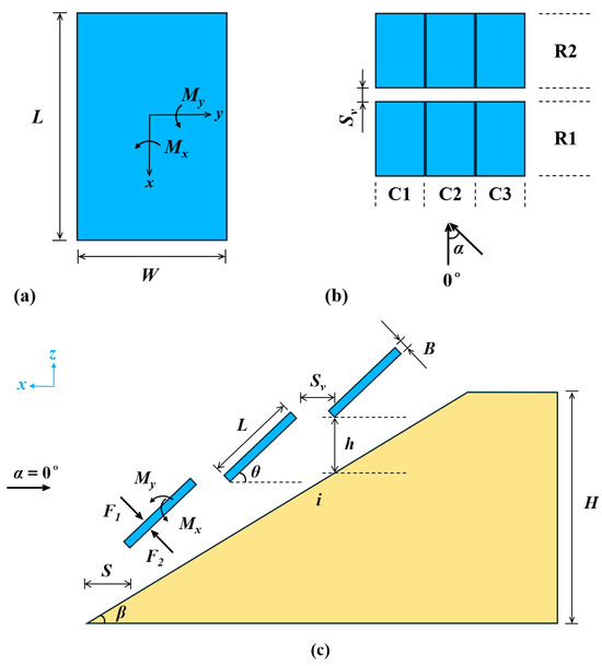
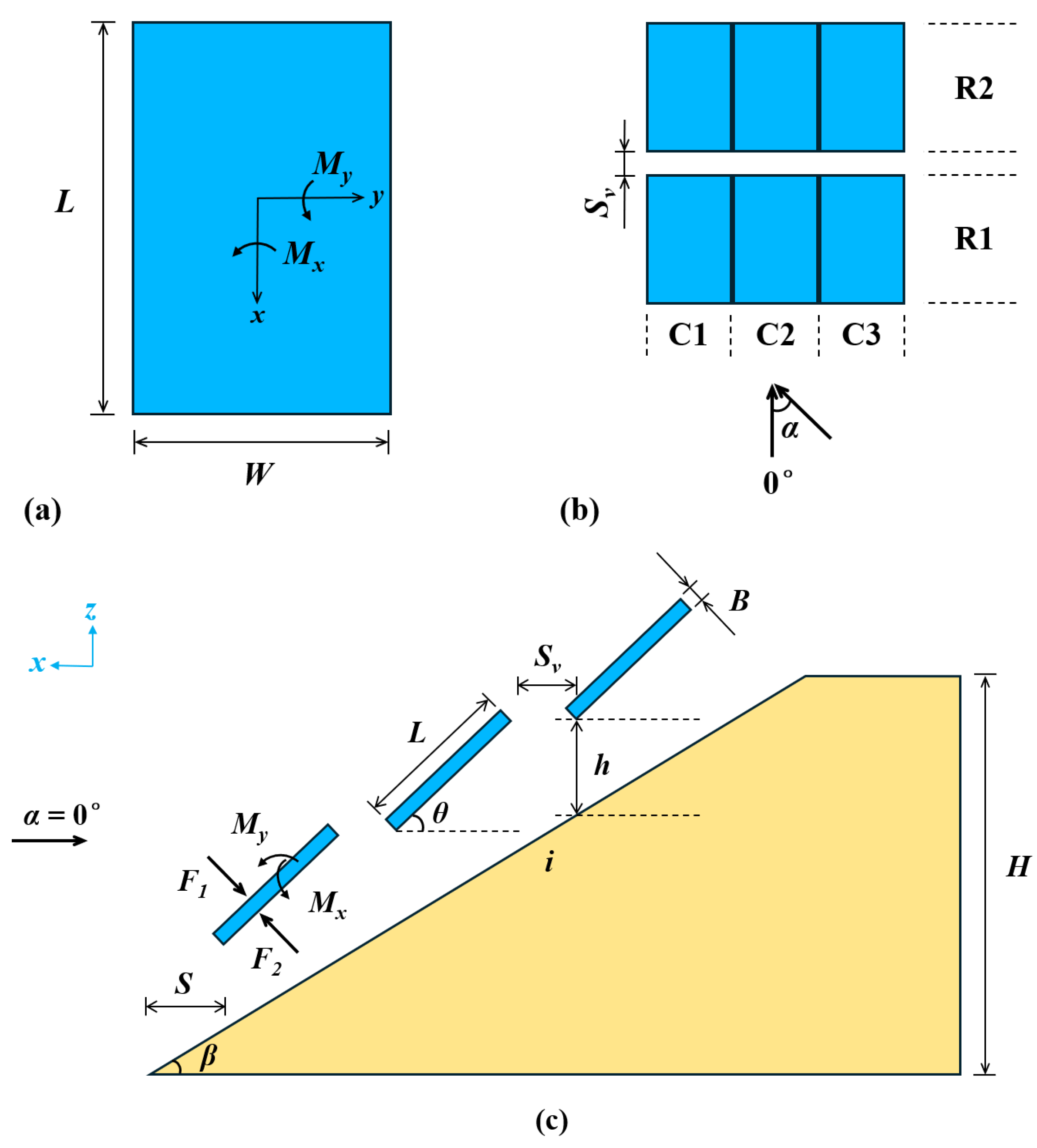
In this study, a 50 m-long highway slope section was used as the basic unit to establish the geometric model of the HSPV system. The selected photovoltaic module dimensions were 2382 mm × 1134 mm × 30 mm. The geometric model and its parameters are shown in Figure 1.
Figure 1.
Schematic of the HSPV model and parameters: (a) Plan view of a photovoltaic module; (b) Plan view of the photovoltaic array; (c) Elevation view of the HSPV system.
In this study, α = 0° was selected as a representative critical direction for conservative assessment of wind loads on HSPV systems, consistent with common practice in PV wind-load studies [15]. Classic embankment-flow observations also indicate that near-normal approach winds can produce pronounced speed-up over slopes [21]; oblique inflows may shift acceleration/deceleration zones and modify wake interactions and are therefore reserved for future extension. The structural parameters of the HSPV system are defined as follows. For the slope: height H and angle β (also expressed as slope i); for a single photovoltaic module: length L, width W, thickness B, and tilt angle θ; for the array layout: lateral spacing Sh, longitudinal spacing Sv, panel height above the ground h, and horizontal distance from the first row of panels to the slope toe S. The naming convention for the photovoltaic array is as follows: the first row along the negative x-axis is denoted as R1, and the first column along the positive y-axis is denoted as C1.
2.2. Computational Parameters
The wind pressure coefficient reflects the distribution of static pressure on the surface of a structure under steady wind, which is calculated by Equation (1):
where μsi is the pressure coefficient at measurement point i; wi is the net wind pressure at point i, defined as the difference between the measured wind pressure at the point and the atmospheric static pressure of the incoming flow; is the reference mean wind speed, generally taken as the average wind speed at 10 m height; and ρ is the air density.
The shape coefficient, also known as the mean wind pressure coefficient, is calculated as the area-weighted average of the pressure coefficients across all measurement points on the surface by Equation (2):
where μs is the module-level shape coefficient obtained by area integration of the pressure distribution, Ai is the area corresponding to measurement point i, and A is the total surface area. For an entire photovoltaic panel, the overall shape coefficient can be expressed as the difference between the upper and lower surfaces, which is calculated by Equation (3):
where PU and PD represent the wind pressures on the upper and lower surfaces, respectively.
The non-uniform distribution of wind loads induces bending moments on the photovoltaic panel. The moment coefficient about the y-axis is calculated by Equation (4):
where CMy is the moment coefficient about the y-axis, and My is the bending moment about the y-axis.
2.3. Computational Domain
Based on previous numerical simulation studies on wind loads of photovoltaic arrays and highway wind environments [26,27,28], the computational domain for all models in this study was designed according to the following principles:
- (1)
- The distance from the domain inlet to the model should be no less than 5 × l(z)max;
- (2)
- The distance from the model to the domain outlet should be no less than 15 × l(z)max;
- (3)
- The distance from the model to the lateral boundaries of the domain should be no less than 5 × l(z)max, or the domain width should be no less than 4 × l(y)max;
- (4)
- The domain height should be no less than 9 × l(z)max.
Here, l(z)max and l(y)max denote the maximum dimensions of the numerical model in the z- and y-directions, respectively.
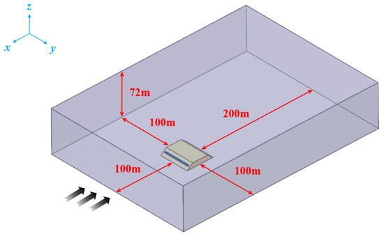
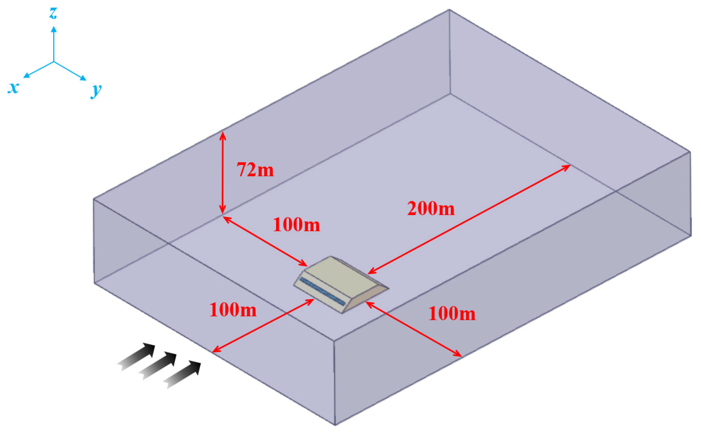
As an example, a slope model with an embankment height of 8 m and a slope ratio of 1:1.25 was considered. The photovoltaic modules were arranged in a single row without gaps, with tilt angles aligned with the slope, a panel height h = 1 m, and a horizontal distance from the slope toe S = 4 m. The computational domain used for this model is shown in Figure 2. The blockage ratio of this model is 2.22%, satisfying the requirement of not exceeding 3%. All other models also meet the blockage ratio criteria.
Figure 2.
The computational domain of Model 10.
2.4. Numerical Simulation Parameters
In this study, the wind loads on HSPV systems were simulated using a three-dimensional steady-state numerical approach. The computational model was built at a full scale (1:1). The averaged Reynolds equations were solved using the SST k-ω turbulence model, which is widely used for equilibrium atmospheric boundary layer simulations and near-wall external flows [29]. The pressure–velocity coupling was handled using a coupled scheme in ANSYS Fluent, and second-order discretization was adopted for the transport equations. The near-wall mesh resolution was controlled to achieve y+ ≈ 1 (typically within 0.5–2.0) for the first-layer wall cells.
The inlet boundary conditions included the mean wind velocity profile , the turbulent kinetic energy profile k(z), and the specific dissipation rate profile ω(z), and their calculation methods are presented in Equations (5)–(7):
where is the wind speed at the standard reference height of 10 m, taken as 20 m/s, corresponding to a Beaufort scale 8 wind; Cμ is an empirical constant, taken as 0.09.
The outlet was specified as a pressure outlet with a pressure of 101,325 Pa, representing standard atmospheric conditions. The top and lateral boundaries were treated as symmetry planes. The highway slope, photovoltaic modules, and ground were defined as no-slip walls to isolate the topographic effects in a consistent manner.
2.5. Validation of the Modeling Approach
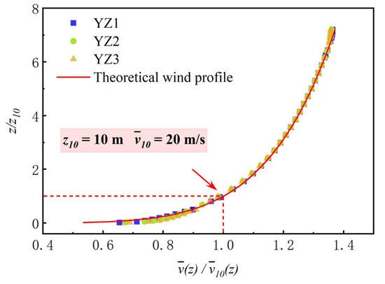
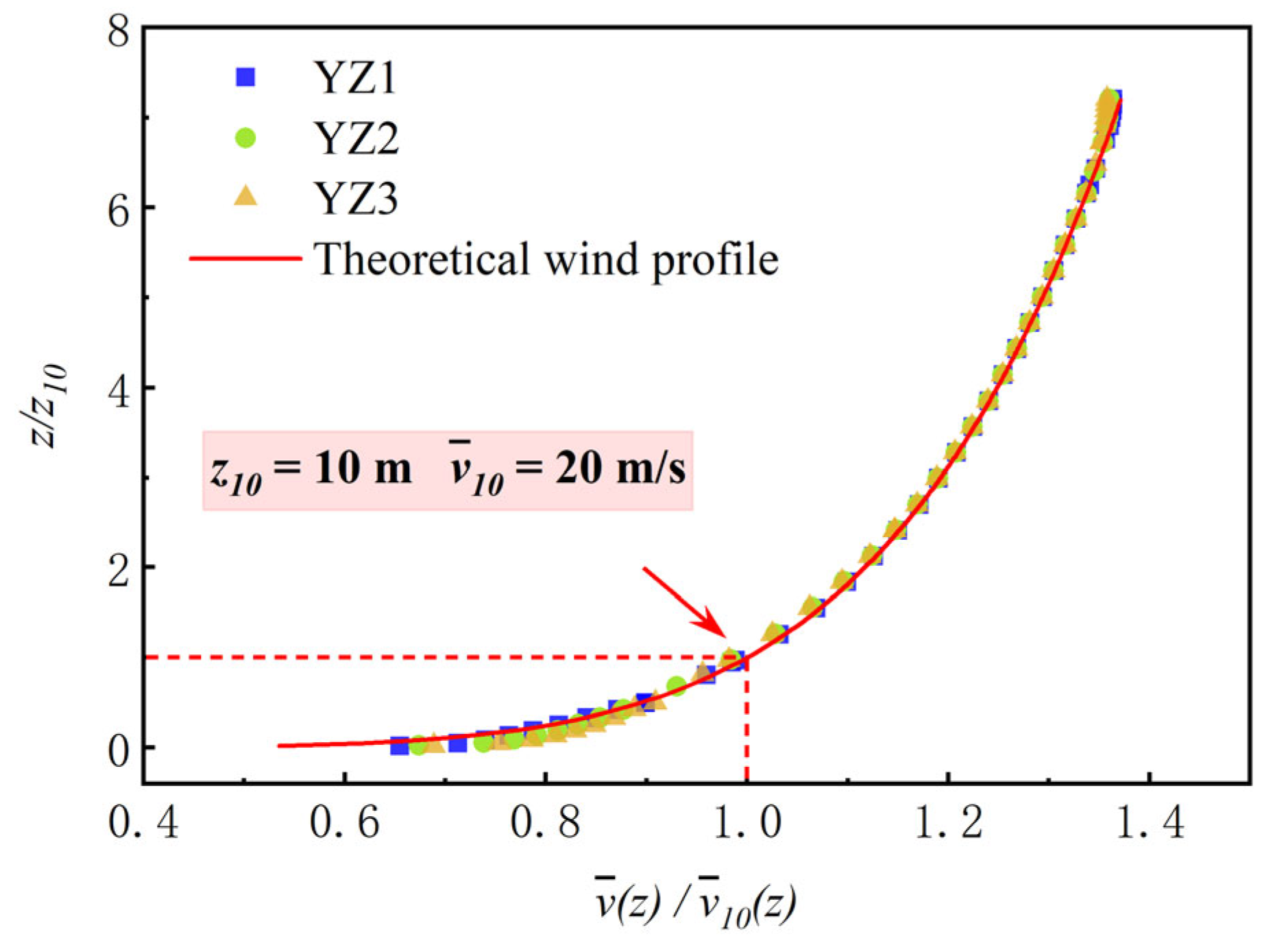
First, the computational domain was divided into four equal sections by introducing three analysis planes perpendicular to the incoming wind direction, labeled YZ1, YZ2, and YZ3. The agreement between the numerical and theoretical velocity profiles was examined for the empty flow field without any model, as shown in Figure 3. The numerical results were in good agreement with the theoretical wind velocity profile in terms of overall trends, with relative errors controlled within 5%. The velocity profiles at different locations are highly consistent, indicating that the inlet wind field is sufficiently developed and remains stable within the computational domain.
Figure 3.
Comparison between numerical and theoretical wind velocity profiles.
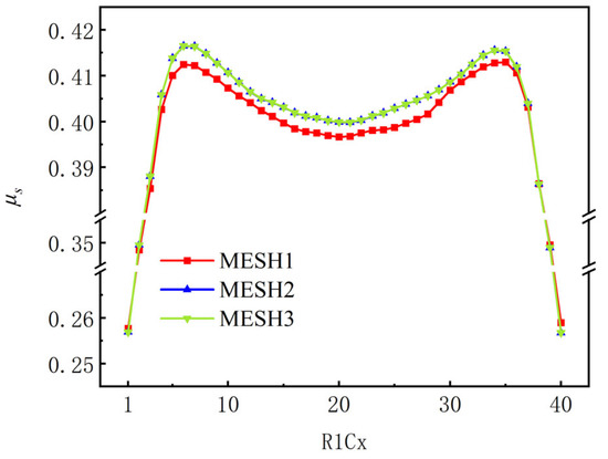
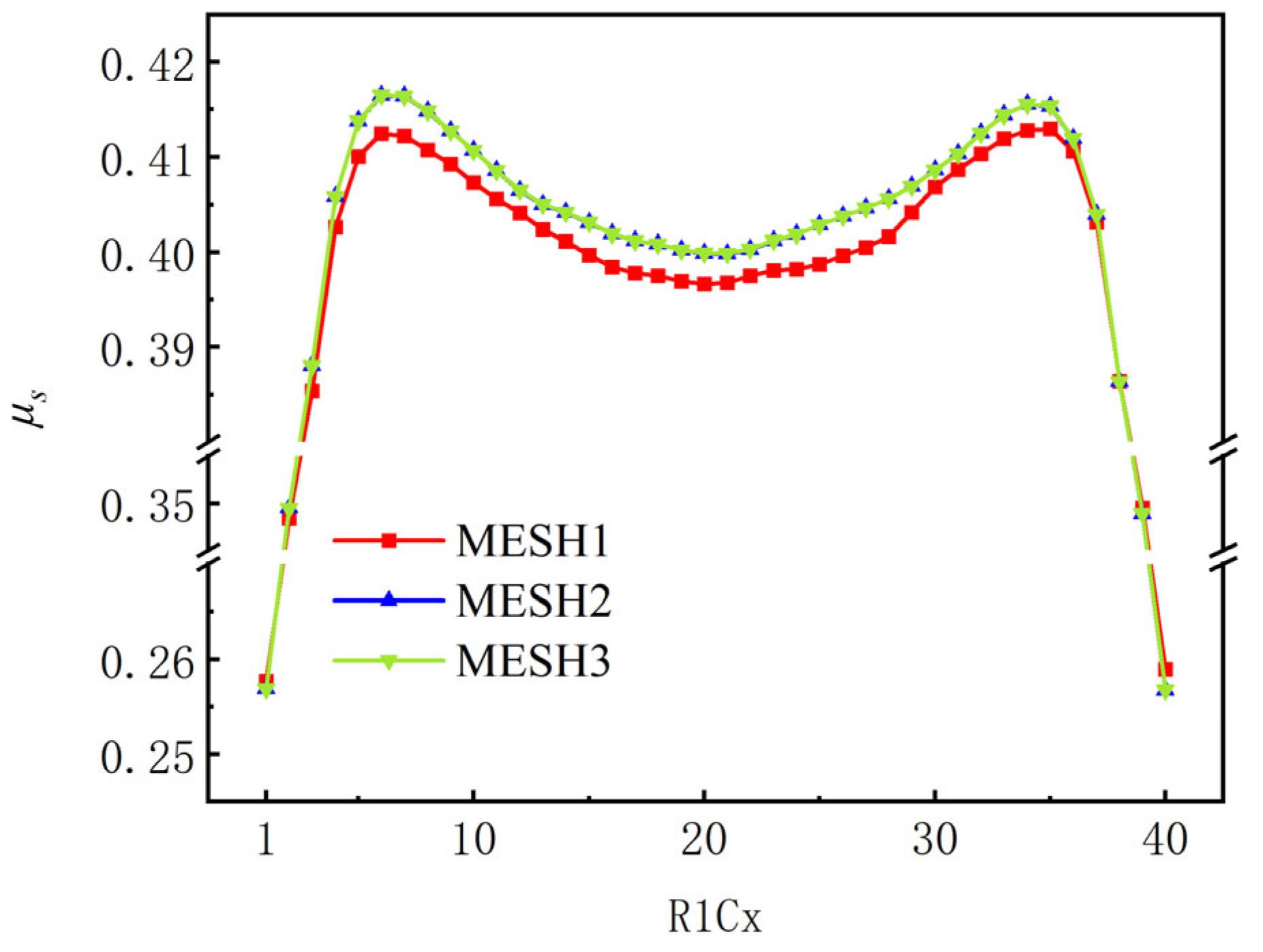
Second, a mesh sensitivity analysis was conducted for the HSPV model. Three mesh schemes were constructed, including a coarse mesh (MESH1), a medium mesh (MESH2), and a fine mesh (MESH3), with the parameters listed in Table 1. The quality of all three mesh schemes satisfies the basic requirements for engineering CFD simulations. The distribution of shape coefficients for individual photovoltaic panels within the array is shown in Figure 4. The results indicate that three mesh schemes exhibited highly consistent distribution trends. As the mesh resolution increased, the shape coefficient gradually converged, indicating reduced sensitivity to mesh refinement and good mesh independence of the numerical results.
Table 1.
Mesh division scheme.
Figure 4.
Shape coefficients of three mesh schemes.
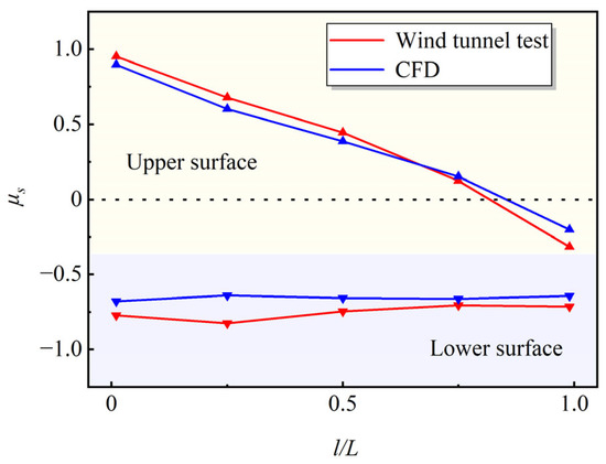
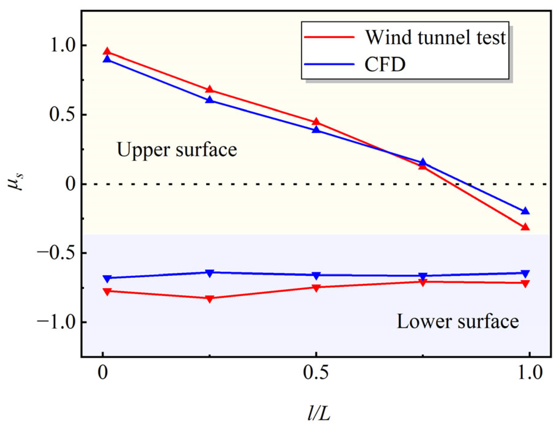
Third, photovoltaic panels with existing wind tunnel test results from literature [16] were selected as reference models. Following the aforementioned numerical simulation method, steady-state flow simulations were conducted. The distributions of shape coefficients along the windward direction for the upper and lower surfaces, obtained by both methods, are shown in Figure 5. It can be observed that the numerical simulation results closely align with the wind tunnel test results in terms of trend lines, peak values, and characteristic points. The numerical simulation method established in this study can effectively reflect the distribution patterns of wind loads on photovoltaic panel surfaces.
Figure 5.
Comparison of wind tunnel test and numerical simulation results.
3. Evolution of Roadside Wind Environment
3.1. Geometric Parameters and Monitoring Configuration
Embankment height and slope ratio are critical geometric parameters for highway slopes and play an important role in shaping the local wind environment. In this study, seven typical slope configurations were selected, as summarized in Table 2.
Table 2.
Geometric parameters of HSPV slope models.
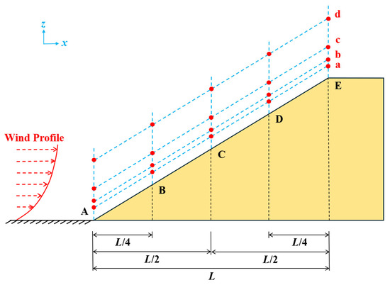
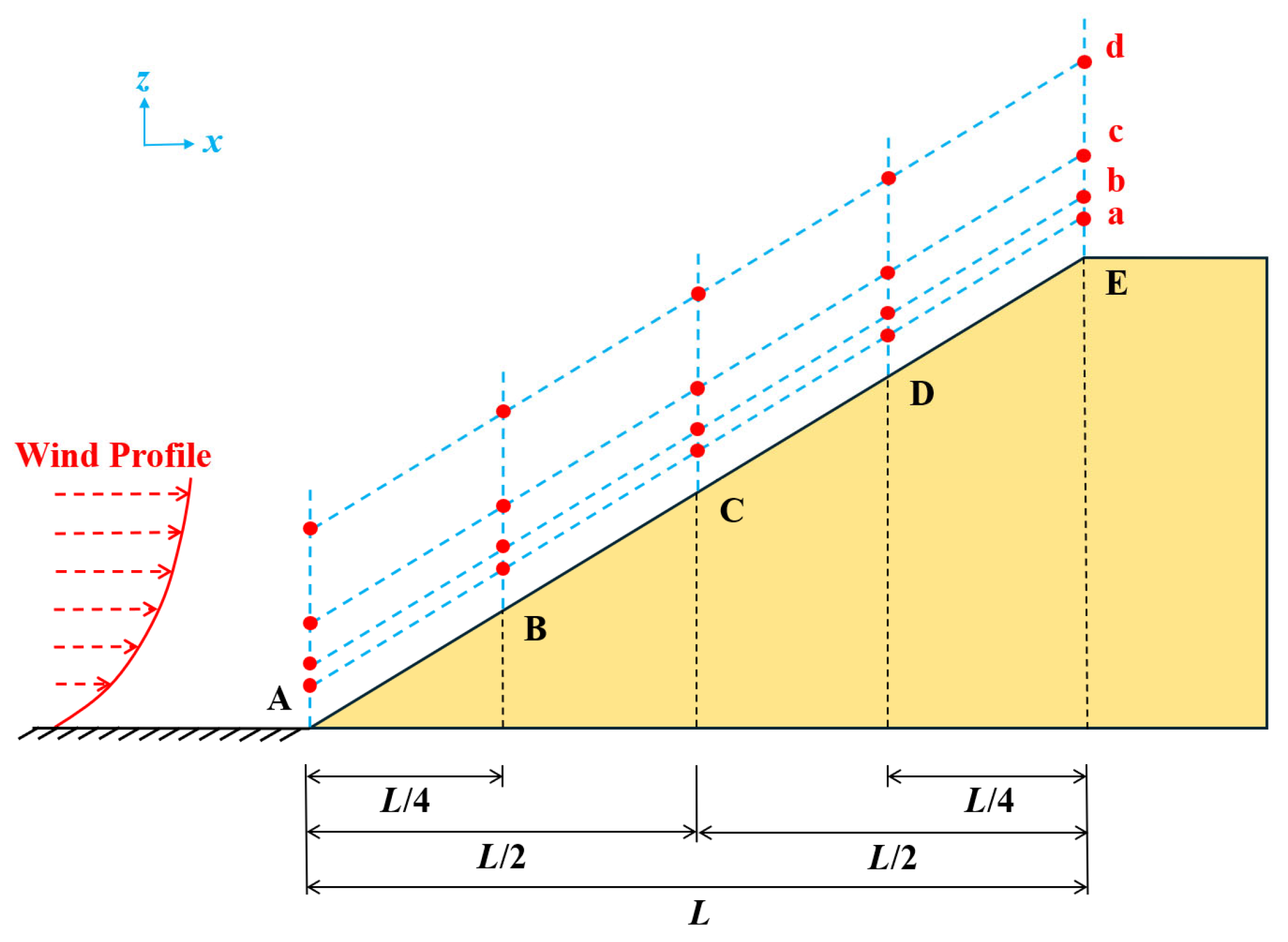
Five monitoring points, labeled A, B, C, D, and E, were placed on the slope surface to observe wind profile characteristics. Furthermore, four different heights (a, b, c, d) above each monitoring point were chosen as characteristic points to analyze the mean wind speed variation with height. The monitoring configuration is shown in Figure 6.
Figure 6.
Schematic diagram of monitoring locations.
3.2. Wind Profile Characteristics
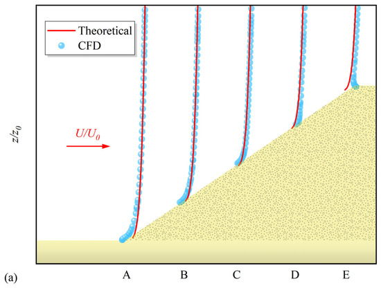
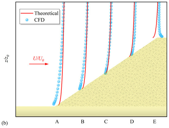
The theoretical wind profile describes the vertical variation in wind speed under ideal flat terrain conditions. In contrast, the wind profiles extracted at monitoring points on the slope reflect disturbances of the approaching flow induced by the embankment geometry. A comparison between the theoretical and simulated profiles enables a direct identification of wind speed amplification or reduction under different slope configurations. The along-slope evolution of the wind profiles is consistent across cases, as illustrated by Model 1 and Model 7 in Figure 7.
Figure 7.
Evolution of wind profiles: (a) Model 1; (b) Model 7.
The differences between cases are reflected in the degree of separation between the simulated and theoretical wind profiles. To quantify the topographic influence on the wind profile, a wind profile deviation δ is defined to represent the discrepancy between the actual and theoretical wind profiles, as expressed in Equation (8):
where U(z) is the wind speed at height z above the ground under topographic influence, and U0(z) is the wind speed at the same height over flat terrain without topographic influence. For each monitoring point, the maximum deviation δmax is reported as a concise measure of the peak departure between the simulated and theoretical profiles.
Representative variations are observed between the simulated and theoretical wind profiles. The profiles at monitoring points A to D generally conform to the theoretical exponential law and increase monotonically with height, whereas the profile at point E exhibits a localized deviation with an opposite trend.
Specifically, at point A near the slope toe, the simulated wind profile deviates markedly from the theoretical exponential profile in the near-ground region. The corresponding δmax values at point A are 876.27% for Model 1 and 1120.83% for Model 7. At low heights, the simulated wind speed is significantly lower than the theoretical value, indicating a local deceleration effect on the windward side of the slope. As height increases, the two profiles gradually converge and eventually coincide at higher elevations, suggesting that the deceleration effect near the slope toe is mainly confined to the region close to the slope surface.
As the monitoring location moves upward along the slope to points B, C, and D, the simulated wind profiles exhibit a progressive rightward shift. At the same height, wind speeds continuously increase and exceed the theoretical values within a certain height range, forming a rightward bulging of the simulated profiles in the low- to mid-height region. The peak deviation δmax further quantifies this slope-induced acceleration effect. For Model 1, δmax is 71.64%, 6.49%, and 38.92% at points B, C, and D, respectively; for Model 7, the corresponding values are 91.98%, 16.26%, and 39.47%. This behavior reflects the acceleration of airflow along the slope, leading to a pronounced wind speed amplification zone above the middle and upper sections of the slope.
At monitoring point E, the deviation between the simulated and theoretical wind profiles in the near-ground region is most pronounced, indicating that slope-induced acceleration reaches its maximum near the crest. The peak deviation δmax at point E is 59.37% for Model 1 and 71.16% for Model 7, providing a quantitative indication of the maximum separation in the near-ground layer. In the lower height range, an inverse pattern is observed, characterized by wind speed amplification near the ground and partial recovery at mid-to-upper heights. Consequently, at low heights close to the slope crest, the simulated wind speed exceeds the theoretical value, locally deviating from the monotonic increase predicted by the exponential law.
Overall, in the upper region far from the slope surface, the simulated wind profiles at all monitoring points show good agreement with the theoretical profile, indicating that the slope has a limited influence on the mean wind speed in the main flow layer. In contrast, in regions close to the slope surface, particularly near the slope toe and crest, the simulated wind speeds exhibit clear local amplification or attenuation relative to the theoretical profile. This demonstrates that the topographic effect is mainly concentrated in the near-ground layer adjacent to the slope. Since this region coincides with the typical installation zone of HSPV systems and other roadside structures, such structures are directly affected by wind profile distortions induced by slope topography.
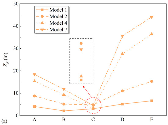
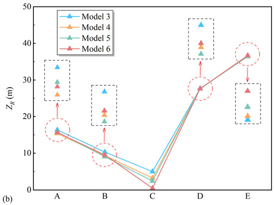
While δ and the corresponding peak deviation provide a direct measure of the maximum departure, it is also necessary to characterize the vertical extent over which the profile is affected by topography. When δ remains below 5% for ten consecutive sampling heights above a reference height ZR, the wind profile is considered to have essentially recovered to the undisturbed boundary-layer characteristics above ZR. The 5% threshold is adopted as a practical recovery tolerance, consistent with the inlet boundary-layer verification accuracy level (errors < 5%) used in this study. Accordingly, ZR is defined as the onset height unaffected by topography, or the wind profile recovery height. The values of ZR for all monitoring points under different slope conditions are shown in Figure 8.
Figure 8.
Wind profile recovery heights: (a) Cases with constant slope ratio and varying slope heights; (b) Cases with constant slope height and varying slope ratios.
For the case group with constant slope ratio and varying slope heights (Models 1, 2, 4, and 7), where the slope ratio is maintained at 1:1.25, the wind profile ZR at monitoring points A to E shows a clear increasing trend as the embankment height rises from 2 m to 10 m. At the slope toe (point A), ZR increases from 4.1 m in Model 1 to 18.4 m in Model 7, indicating that as the slope height increases, the near-ground wind profile close to the toe requires a greater height to recover to the theoretical distribution, with the actual wind profile remaining below the theoretical profile. ZR at points B and C also increases, from 2.6 m and 4.1 m to 14.3 m and 9.5 m. However, the amount of increase gradually decreases, because the slope-induced acceleration causes the actual wind profiles to more closely follow the theoretical values. Compared with lower embankments, such as in Model 1, ZR is longer for higher embankments like Model 7, reducing the relative differences in ZR. For the upper slope points D and E, however, the differences in ZR increase again, with a gap of over 30 m between Model 7 and Model 1, as the slope-induced acceleration causes the actual wind speed to exceed the theoretical values.
Overall, when the slope ratio is constant, increasing the slope height not only amplifies the local distortion of the near-ground wind profile but also significantly raises ZR, expanding the influence range of topographic effects. Moreover, compared with the mid-slope region, locations near the slope toe and crest are more sensitive to changes in slope height.
For the case group with constant slope height and varying slope ratios (Models 3, 4, 5, and 6), with the embankment height fixed at 8 m, the slope ratio gradually decreases from 1:1 to 1:1.75. ZR trends at all monitoring points are consistent across cases, generally decreasing at first and then increasing. Due to the deceleration effect near the slope toe, the actual wind profile at point A is significantly lower than the theoretical profile, requiring a greater ZR for the wind speed to recover. As airflow climbs along the slope and accelerates, the deviation at points B and C decreases. With the accumulation of the acceleration effect, the deviation increases again, reaching its maximum at the slope crest (point E). The differences in ZR among the four cases at the same monitoring point are small. This indicates that ZR of slope wind profiles is less sensitive to slope ratio but highly sensitive to slope height. Near point C, there is a transition in the relative magnitude of the actual and theoretical wind profiles. As shown in Figure 8, as the slope ratio decreases, the wind profile ZR lowers, indicating stronger wind speed recovery capability, although the wind speed variation along the mid-slope becomes more pronounced.
3.3. Mean Wind Speed Characteristics
The HSPV modules are installed within the near-ground region, where wind profiles vary sharply along the slope. Therefore, four representative heights (2 m, 3 m, 5 m, and 10 m) above each monitoring point were selected to analyze the characteristics of the mean wind speed. To account for the amplification or reduction in wind speed caused by topography, a wind speed ratio is introduced to quantify the effect of complex terrain on the mean wind speed, as defined in Equation (9):
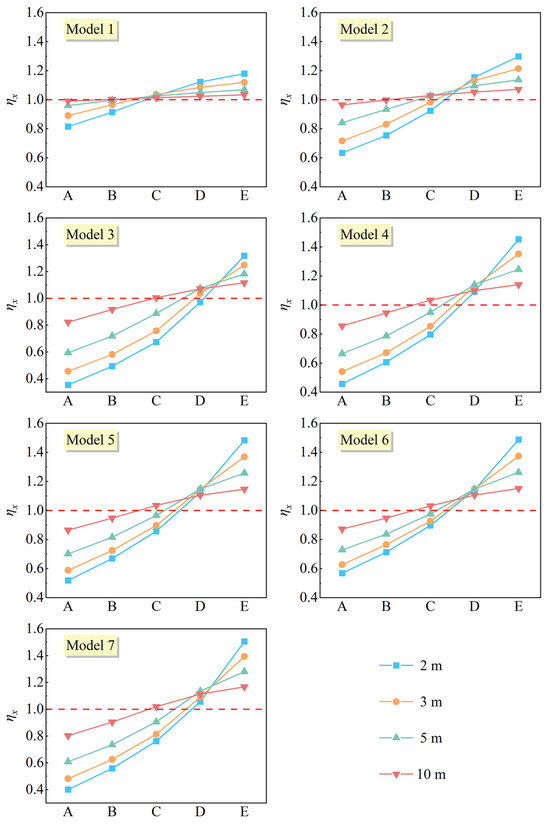
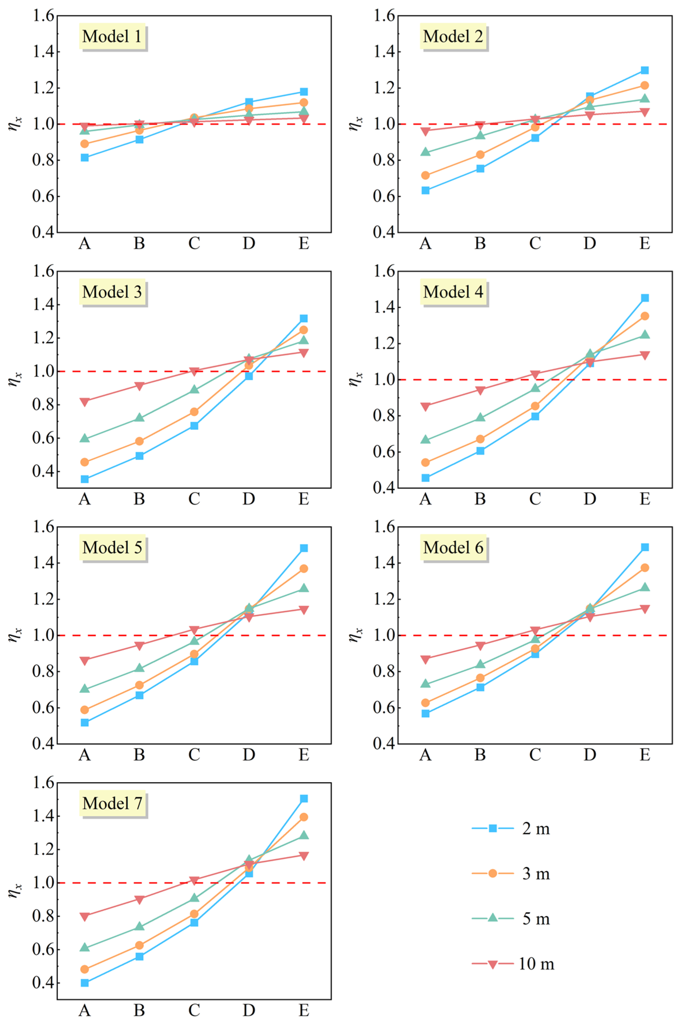
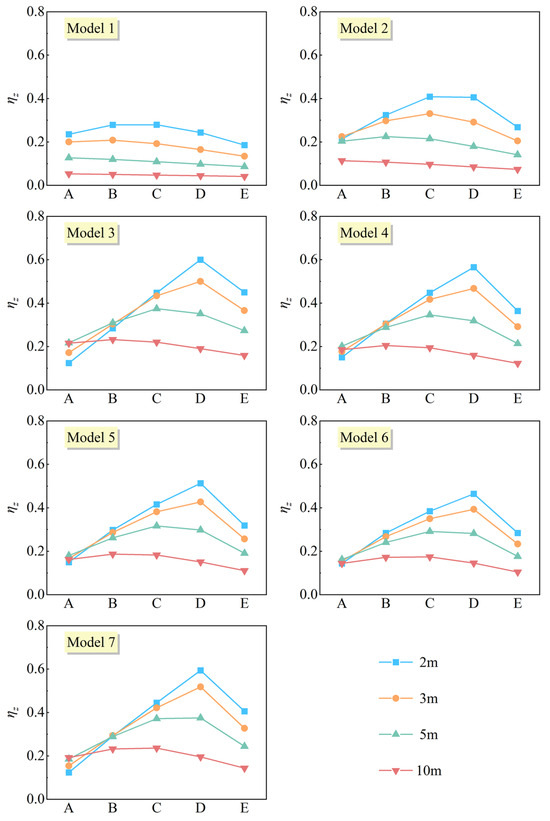
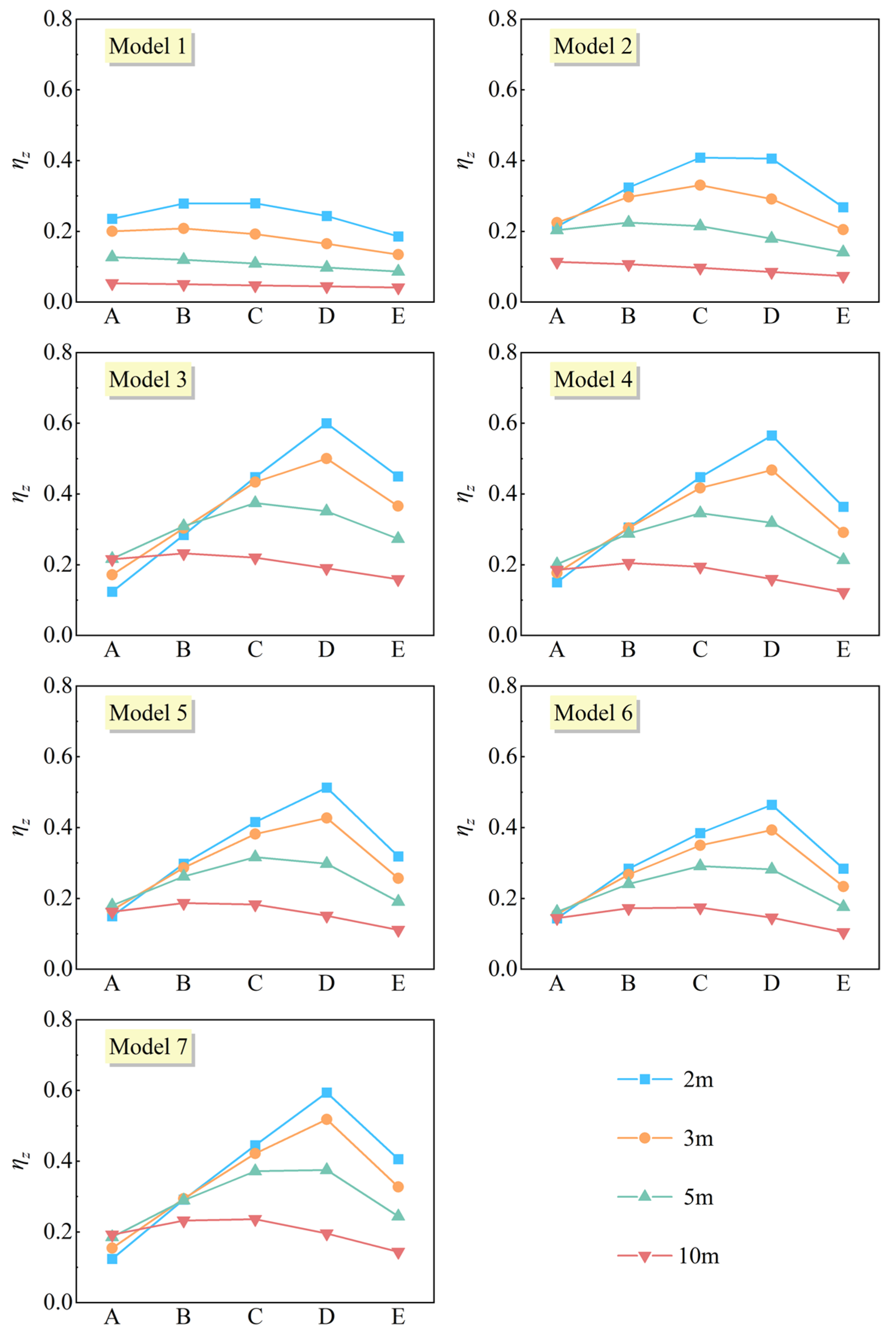
where ηx,y,z denote the wind speed ratios in the x-, y-, and z-directions, respectively, and Ux,y,z(z) represent the corresponding velocity components in the x-, y-, and z-directions at height z above the ground under topographic disturbance. When ηx > 1, the along-wind speed at that height is amplified relative to flat terrain, indicating an acceleration effect; conversely, ηx < 1 signifies a deceleration effect. The crosswind (y) and vertical (z) wind speed ratios reflect the extent of flow deflection and upward motion induced by complex terrain.
Figure 9.
Along-wind (x) wind speed ratio.
Figure 10.
Crosswind (y) wind speed ratio.
Figure 11.
Vertical (z) wind speed ratio.
From the distribution of the along-wind speed ratio ηx, the influence of the highway slope on the mean wind speed exhibits clear spatial stratification. Moving upward along the slope, ηx increases monotonically at all heights, with pronounced differences in the rate of change. At higher elevations far from the slope influence (e.g., 10 m), the ηx at all monitoring points is generally close to 1. This indicates that the mean wind speed in the main flow layer is essentially consistent with the theoretical value over flat terrain. The disturbance induced by slope topography is mainly confined to the near-ground layer. Moreover, a comparison among monitoring points shows that at the slope toe (point A) and the lower-to-middle slope points (B and C), ηx is slightly less than 1 within the 2–5 m height range. This indicates a certain degree of flow deceleration as the airflow approaches the windward slope. Moving upslope to points D and E, ηx gradually exceeds 1 and reaches a peak near the crest, corresponding to the acceleration effect revealed by the wind profiles in Figure 7.
For the case group with a constant slope ratio and varying slope heights (Models 1, 2, 4, and 7; slope ratio 1:1.25), an increase in embankment height leads to an overall increase in the deviation magnitude of ηx at all monitoring points. Under low-embankment conditions, the ηx at heights of 2 m and 3 m show only minor amplification or attenuation at a limited number of locations. As the slope height increases, ηx at heights of 5 m and 10 m near the middle-to-upper slope and the slope crest becomes significantly greater than 1, while ηx at 2 m near the slope toe decreases markedly below 1. This indicates that higher slopes not only enhance the along-wind acceleration above the slope crest but also intensify local near-ground deceleration at the slope toe. Consequently, increasing slope height strengthens the topographic disturbance to the along-wind mean wind speed and extends its influence to higher elevations, consistent with the variation trend of the wind profile recovery height shown in Figure 8.
In the case group with a constant slope height and varying slope ratios (Models 3, 4, 5, and 6), variations in the along-wind speed ratio mainly reflect the influence of slope steepness on the redistribution of the near-ground flow field. As the slope becomes gentler, the deviation of ηx at heights of 2–5 m near the slope toe and the middle slope decreases, indicating a reduction in the deceleration effect at the slope toe. Compared with Model 3, the acceleration effect near the slope crest is more pronounced in the other cases. Nevertheless, as the slope ratio decreases from 1:1.25 to 1:1.75, the differences in the mean wind speed at the crest point E remain relatively small.
Overall, these findings are consistent with the conclusions drawn from the wind profile analysis. Pronounced amplification of the along-wind mean wind speed occurs over the middle-to-upper slope and near the slope crest, whereas a certain degree of attenuation is observed near the slope toe. Moreover, different topographic factors affect the extent and intensity of the topographic influence in different ways. Variations in slope height exert a more significant impact, affecting both the crest acceleration zone and the toe deceleration zone. Whereas the influence of slope ratio is mainly manifested in the deceleration zone near the slope toe.
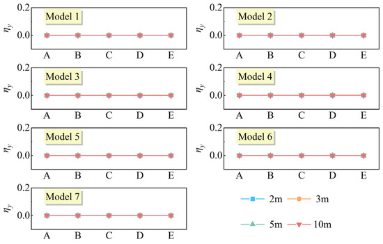
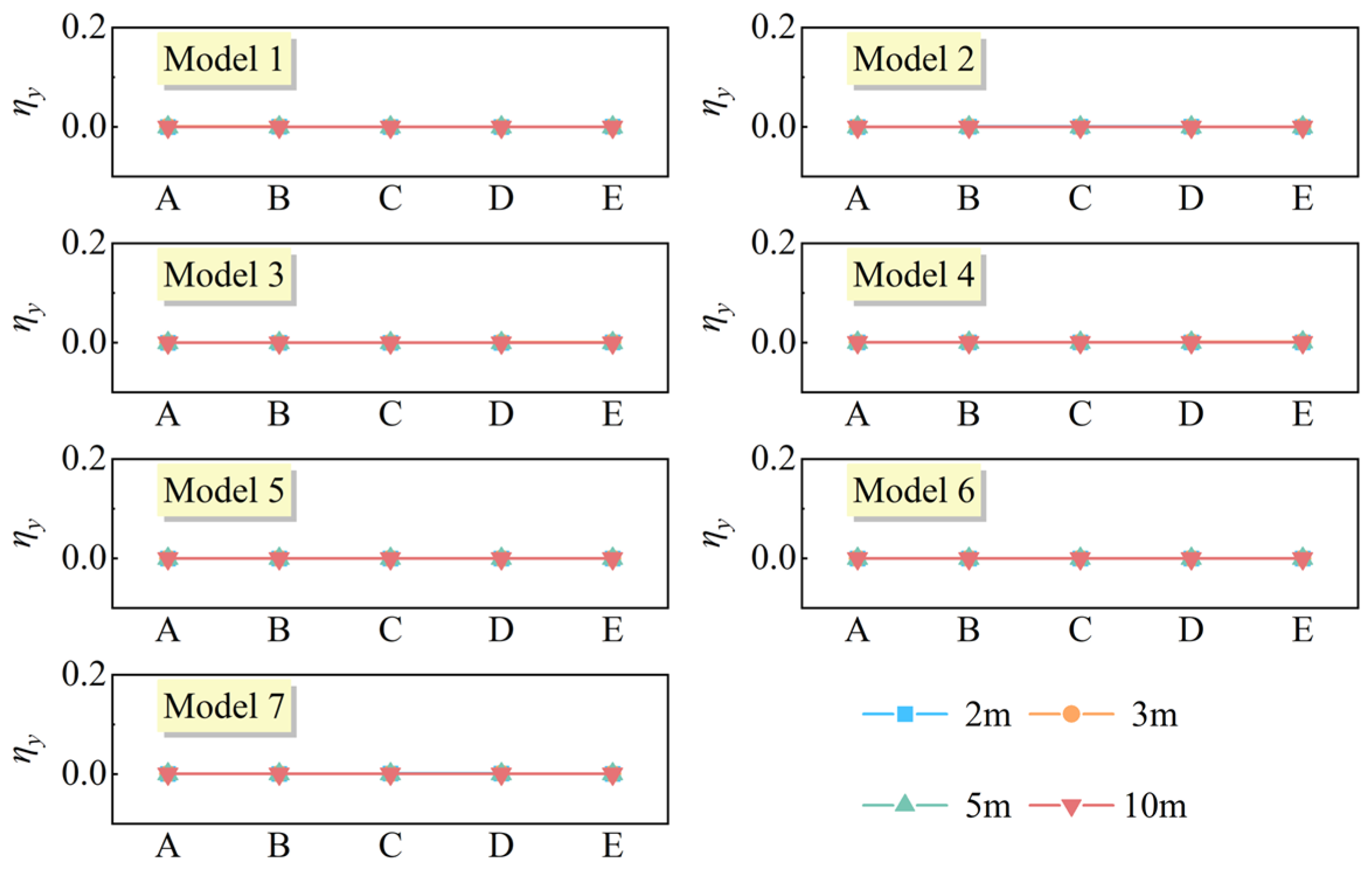
As shown in Figure 10, compared with the along-wind component, ηy at different monitoring points and heights across all cases remains close to zero. This indicates that the overall flow deflection is limited and the incoming flow remains predominantly along the wind direction. When the wind direction angle is 0°, the topography has a negligible effect on the crosswind mean wind speed.
As shown in Figure 11, ηz is generally small across most heights and decreases with increasing height. The vertical component of the mean wind speed is much smaller than the along-wind component. At monitoring points near the slope toe and the middle-to-upper slope, ηz slightly increases within the 2–5 m height range, reflecting an upward deflection of the airflow along the slope. Near and above the slope crest at point E, ηz decreases at certain heights, corresponding to the downward deflection after the flow passes the crest. This phenomenon becomes more pronounced as the slope height increases. When the slope ratio becomes gentler, the local peak of ηz is reduced. This indicates that a gentler slope can lessen flow deflection and thereby weaken the topographic effect on the vertical mean wind speed.
4. Wind Loads on HSPV Systems
4.1. Case Parameters
Under identical inlet boundary conditions and a consistent numerical modeling approach, eight representative slope configurations were selected for investigating the wind loads acting on the photovoltaic arrays. Each array consists of 3 × 40 photovoltaic modules (3R40C). This configuration enables the analysis of interaction effects among multiple rows, including mutual shielding and wake superposition under slope topography. The specific values and combinations of slope structural parameters and photovoltaic configuration parameters are listed in Table 3.
Table 3.
Geometric parameters of HSPV slope models.
4.2. Influence of Slope Gradient on Wind Loads Acting on HSPV Systems
- (1)
- Flow Field Analysis
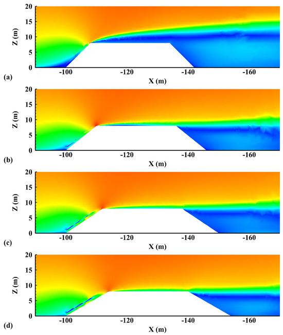
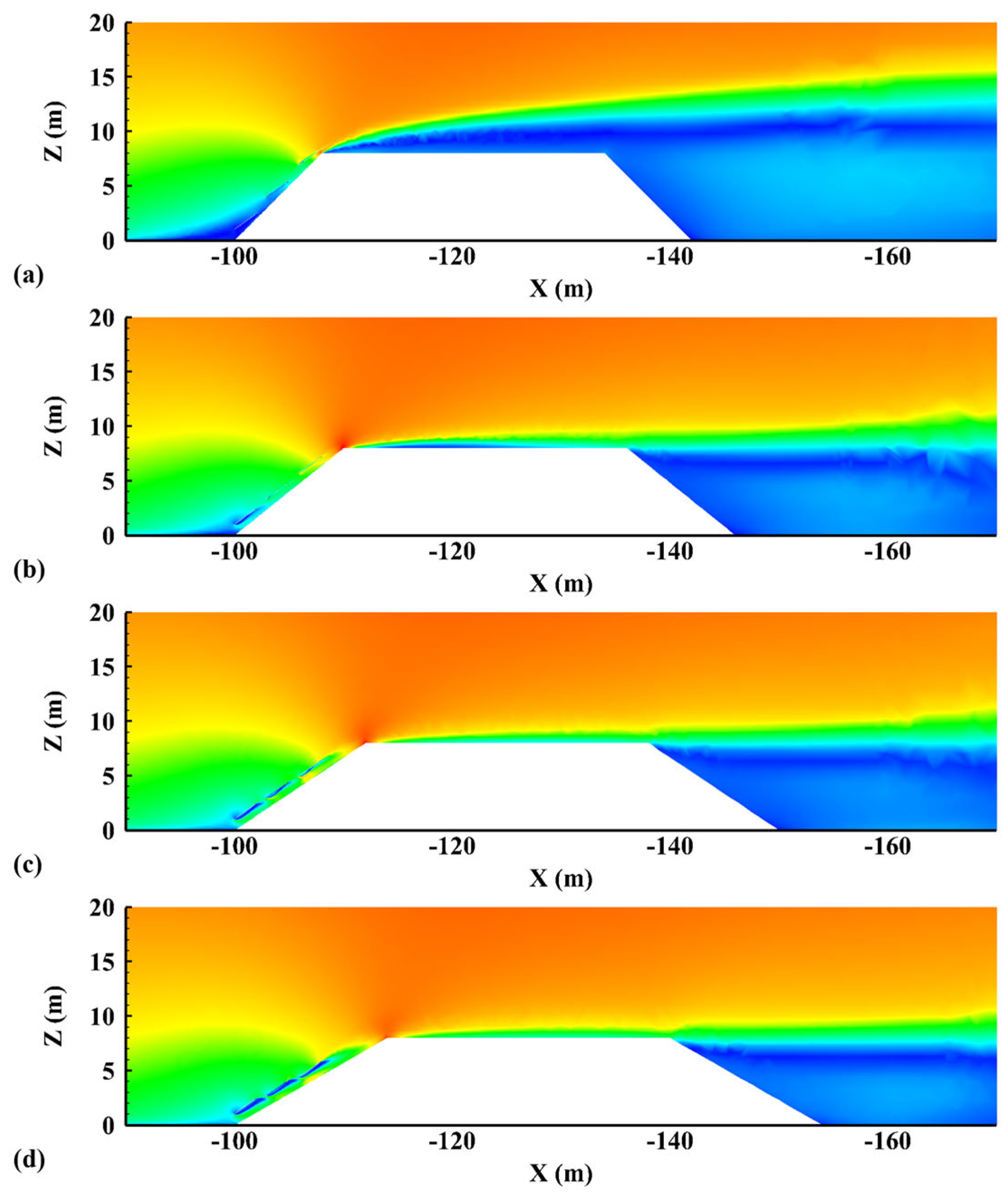
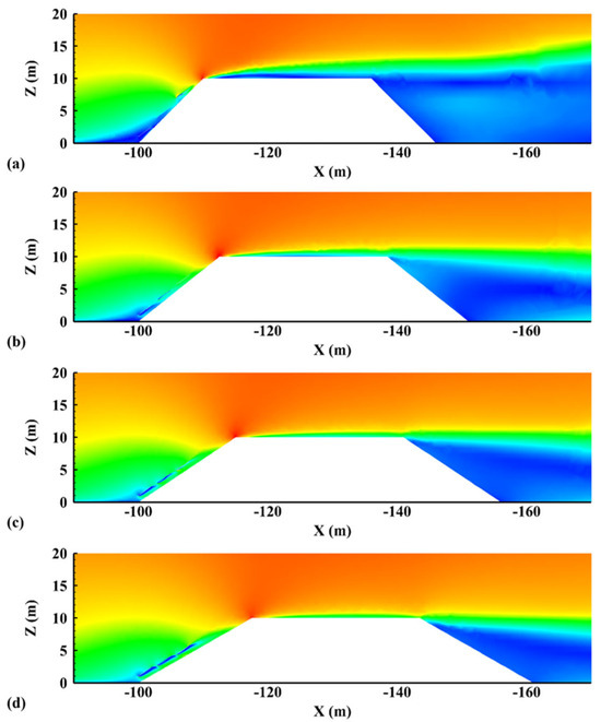
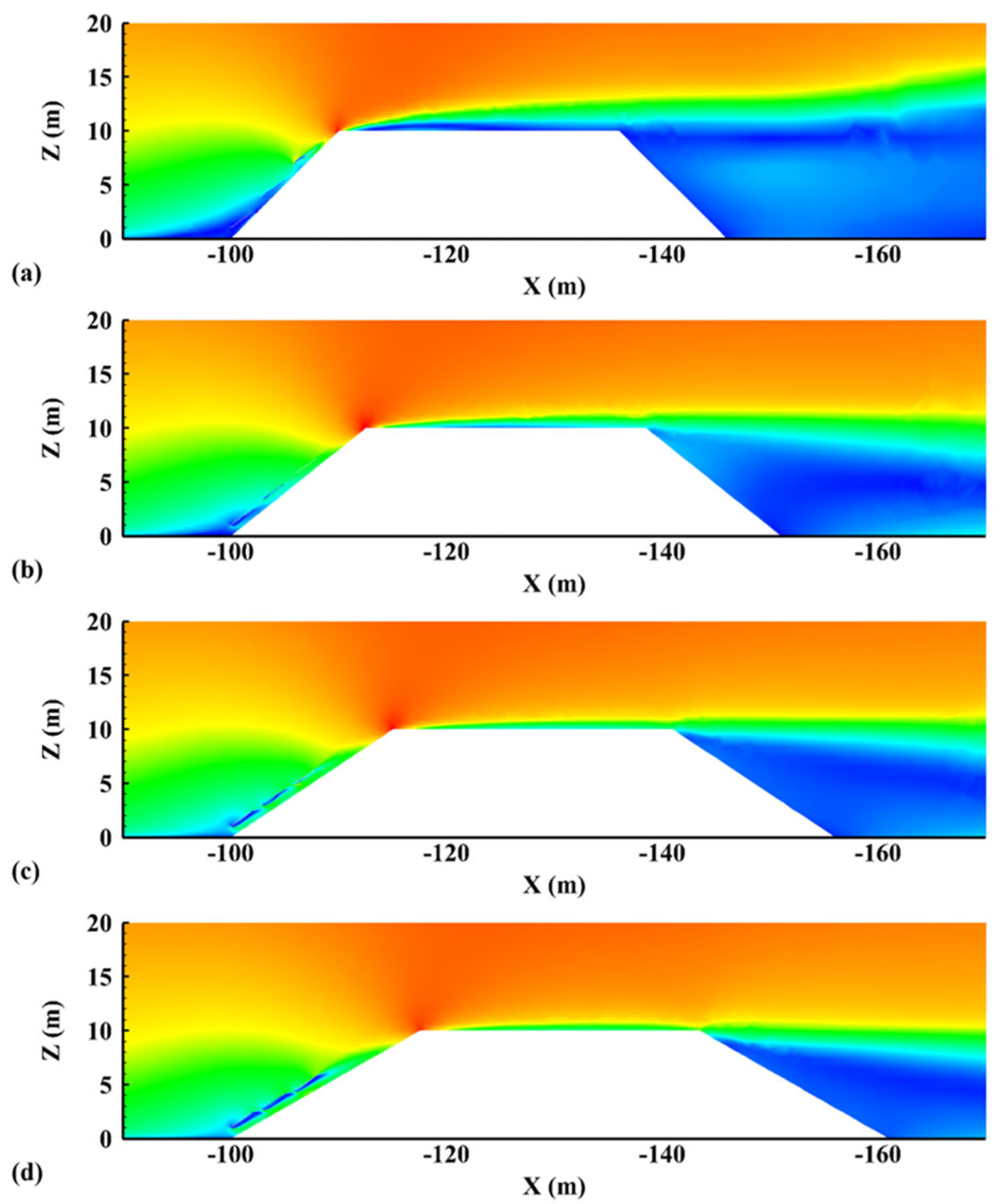
Under the influence of slope topography, the along-wind central section (Y = 125 m) was selected to examine how slope gradient affects the flow field around the photovoltaic arrays. The contours of mean wind speed on the Y = 125 m cross-section are shown for four slope gradients, with the slope height fixed at 8 m, as illustrated in Figure 12. Panels (a) to (d) correspond to slope ratios of 1:1, 1:1.25, 1:1.5, and 1:1.75, respectively.
Figure 12.
Contours of mean wind speed on the Y = 125 m section: (a) Model 8; (b) Model 9; (c) Model 10; (d) Model 11.
Overall, under the combined effects of the photovoltaic arrays and slope topography, the flow field exhibits a stable and representative pattern. This pattern can be summarized as deceleration near the slope toe, acceleration along the slope surface, velocity amplification near the slope crest, and wake development on the leeward side. The approaching flow first experiences local deceleration and streamline uplift near the windward slope toe. It then accelerates along the windward slope, forming a distinct acceleration zone, followed by a sharp increase in the velocity gradient near the slope crest. After passing over the crest, a stratified flow structure develops in the crest and downstream regions, characterized by a high-speed core flow above and a low-speed near-surface layer below. The low-speed region mainly adheres to the slope surface and extends over the photovoltaic array, gradually expanding downstream, while the high-speed core flow remains above it.
For steeper slopes (1:1), the shear layer between the high-speed core flow and the near-wall low-speed region exhibits more pronounced upward displacement, and the downstream low-speed region becomes thicker. A steeper slope introduces a sharper geometric turning of the near-ground streamlines, which promotes stronger shear-layer development and enhances the interaction between terrain-induced flow adjustment and array wakes. This suggests that more pronounced geometric discontinuities are more likely to trigger shear-layer development and intensify wake superposition effects. As the slope becomes progressively gentler (transitioning from 1:1.25 to 1:1.5 and 1:1.75), the acceleration process along the windward slope becomes smoother, while the uplift magnitude and thickness of the shear layer near the slope crest are correspondingly reduced. The upper boundary of the low-speed region shifts downward overall and remains closer to the area above the slope toe, and its downstream extension shows a converging trend. Meanwhile, the coverage of the high-speed core flow expands. This indicates that gentler slopes are more conducive to maintaining attached flow development along the slope and to weakening strong separation and shear structures near the crest. Thereby, the spatial non-uniformity of wind speed within the array region can be reduced. This smoothing of the acceleration and shear structures provides a more uniform inflow to the array, thereby shifting the load response from terrain-dominated separation effects to wake-dominated row-to-row interactions. At the same time, as the slope ratio decreases, the extent of the low-speed region beneath the arrays increases.
In addition, with the tilt angle fixed at 35° and Sv = 1 m, the row-to-row interaction is mainly governed by wake recovery versus wake superposition; under slope-induced stratified flow, the reduced recovery within the near-ground layer makes the rear rows more sensitive to local acceleration and suction amplification. Consistent with Su [17] and Jiang [18], the tilt angle primarily affects the separation tendency and suction level on the upper surface, whereas the longitudinal spacing controls the wake interaction strength between adjacent rows.
Overall, the stratified velocity structure essentially reflects the coupling between topographic effects manifested by slope-induced acceleration and deceleration and array effects manifested by module shielding and wake superposition.
- (2)
- Shape Coefficient and Moment Coefficient
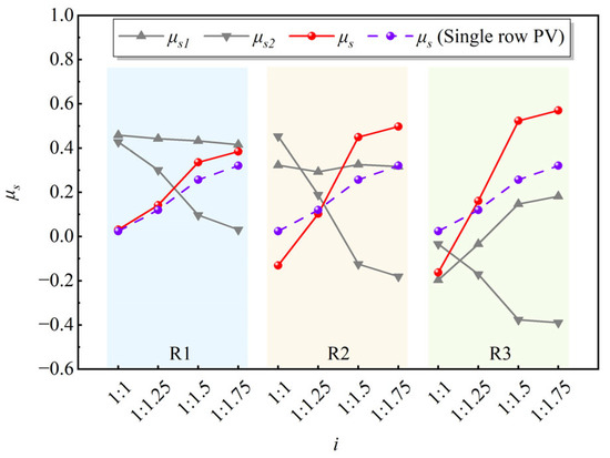
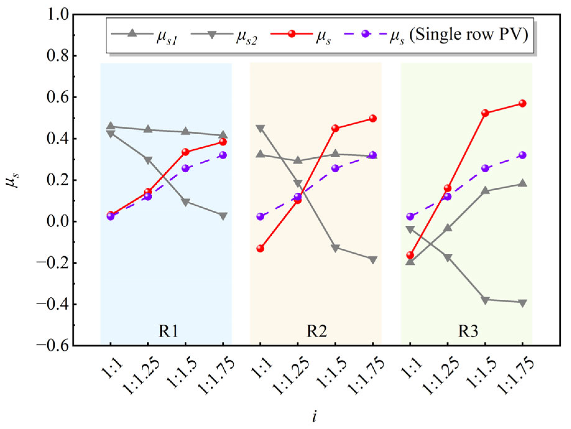
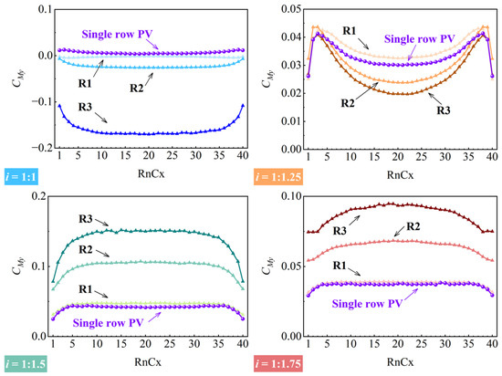
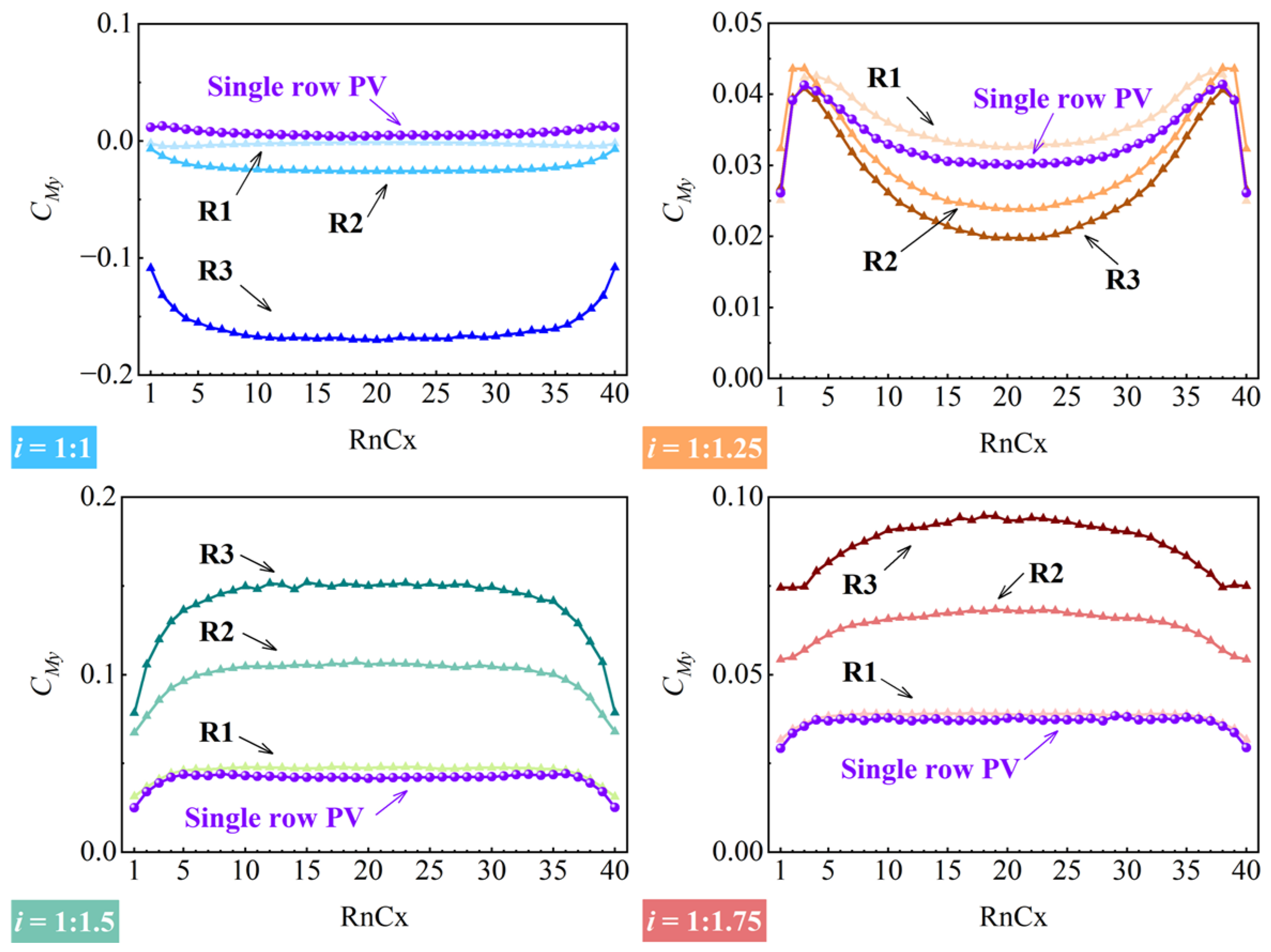
The shape coefficients of the upper and lower surfaces of each row in the photovoltaic array, μs1 and μs2, as well as the row-averaged μs and the average CMy, were compared with those of a single-row photovoltaic array under the same topographic conditions. The results are shown in Figure 13 and Figure 14.
Figure 13.
μs of single-row and array photovoltaic (Models 8–11).
Figure 14.
CMy of single-row and array photovoltaic modules (Models 8–11).
As shown in Figure 13, the μs of the array exhibits a clear row-wise differentiation with varying slope ratios. As the slope becomes gentler, μs for each row in the array shows a monotonically increasing trend, with i = 1:1.75 corresponding to the most adverse net wind pressure conditions. Physically, gentler slopes tend to maintain a more attached and accelerated flow over the array region, which increases the effective dynamic pressure above the modules and can enlarge the net pressure difference reflected by μs.
Under the same slope ratio, for gentler slopes (i = 1:1.5 and i = 1:1.75), the array shows an increasing trend of μs from the front row to the rear row. In contrast, steeper slopes exhibit fluctuations or even decreases in μs across rows.
Compared with a single-row configuration, the front row of the array responds most similarly to the reference case. The subsequent rows are more strongly affected by wake superposition, showing greater deviation. Under steep-slope conditions (i = 1:1), the terrain-induced deceleration extends over a larger area, and disturbances in the near-wall low-speed region within the array are intensified. As a result, the rear-row modules experience pronounced velocity deficits and increased wind pressure on their lower surfaces, leading to a more pronounced reduction in μs compared with the single-row configuration. When the slope is reduced to i = 1:1.25, the deceleration effect near the slope toe weakens and the acceleration along the slope strengthens, reducing the difference between the array and the single-row configuration. As the slope further transitions to i = 1:1.5 and i = 1:1.75, the row-to-row differences within the array are re-intensified. The rear rows experience a more adverse combination of pressure differences due to the combined effects of wake superposition and slope acceleration, causing μs to increase with row number and diverge further from the reference values.
Examining the components of μs, the lower-surface shape coefficient decreases with gentler slopes and also shows a progressive reduction from the front row to the rear row across the array. The upper-surface shape coefficient of modules in the same row either fluctuates or decreases as the slope becomes gentler. Similarly, it decreases from front to rear within the array. Overall, the lower-surface shape coefficient is more sensitive to changes in slope ratio and array configuration, playing a dominant role in the overall shape coefficient. This is because the under-module pressure is strongly influenced by near-wall low-speed layers and wake sheltering, which respond directly to changes in slope-induced boundary-layer thickness and row-to-row wake superposition.
These patterns indicate that the effect of slope ratio on the array’s shape coefficient is not simply a matter of altering the overall wind pressure level. Instead, terrain effects modify the organization of the wake structure within the array. This, in turn, influences the pressure distribution on the upper and lower surfaces, ultimately causing the most unfavorable μs to occur in the rear rows. Notably, under steep-slope conditions, attention should be paid to the negative pressure effects on the rear rows, whereas under gentle slope conditions, the positive pressure effects on the rear rows are of greater concern.
From the distribution along the column direction, stable values are observed in the mid-span region of each row (RnC6–RnC35). However, at both ends of the array, all curves exhibit varying degrees of peaks or drops due to three-dimensional flow around the edges. This indicates that edge modules may still constitute critical positions for bending moment response.
Further comparison reveals that the influence of slope ratio on CMy exhibits pronounced zonal characteristics, mainly manifested as amplitude amplification and row-wise differentiation. Specifically, when i = 1:1, the CMy of the single-row photovoltaic module remains weakly positive and close to zero. In contrast, all rows in the array exhibit negative values, with the magnitude of the coefficient increasing significantly with row number. The CMy of R3 is approximately −0.15, which is markedly lower than those of R1 and R2. This indicates that under steep-slope conditions, strong shear and recirculation tend to develop near the slope crest. These flow structures are more likely to interact with the array wakes, leading to a reverse bias of pressure differences along the leading-trailing edge direction for the rear-row modules. In essence, the crest-adjacent shear/recirculation modifies the pressure distribution between the leading and trailing edges, and the effect accumulates downstream as wakes superpose. As a result, the bending moment direction reverses, making the rear rows the more unfavorable locations in terms of bending moment response.
When the slope ratio decreases to i = 1:1.25, the bending moments of both the array and the single row become positive. The CMy of R1 approaches that of the single-row reference case, while those of R2 and R3 decrease slightly with relatively small magnitudes. This suggests that wake shielding primarily acts to reduce bending moments at this slope ratio, and no amplification effect is formed in the rear rows of the array.
As the slope ratio further decreases to i = 1:1.5 and i = 1:1.75, the amplifying effect of slope ratio on the array bending moment becomes dominant and exhibits a stable row-wise ordering. For both slope ratios, CMy increases progressively from the front row to the rear row and is significantly higher than the single-row reference value. Taking i = 1:1.5 as an example, the CMy of the single row is approximately 0.04, whereas those of array rows R1, R2, and R3 are about 0.08 and 0.15, respectively. This indicates a pronounced amplification effect for the rear rows relative to the single-row case.
In summary, the slope ratio not only governs the magnitude of the CMy but also determines the most unfavorable location of the bending moment response. Under steep-slope conditions, opposite bending moment directions are more likely to occur between the front and rear rows of the array. At moderate slope ratios (particularly i = 1:1.5), the bending moment in the rear rows is significantly amplified and reaches the highest positive levels. It demonstrates stronger sensitivity to slope ratio. Therefore, when evaluating slope effects, single-row references or front-row responses alone cannot adequately represent the overall behavior of the photovoltaic array. Instead, the rear rows should be regarded as the key focus for identifying unfavorable slope-induced effects.
4.3. Effect of Slope Height on HSPV Wind Loads
- (1)
- Flow Field Analysis
The contours of mean wind speed on the Y = 125 m section for four different slope ratios with a slope height of 10 m are shown in Figure 15.
Figure 15.
Mean wind speed contours on the Y = 125 m section: (a) Model 12; (b) Model 13; (c) Model 14; (d) Model 15.
By comparing Figure 12 and Figure 15, the effects of slope height on the wind environment can be summarized as follows. In HSPV scenarios, variations in slope height primarily modulate the near-field flow structure by altering the spatial scale of topographic effects. As the slope height increases, the vertical extent of the acceleration zone along the windward slope increases, and the velocity gradient near the slope crest becomes more pronounced. Meanwhile, the low-speed wake region on the leeward side expands both in height and downstream extent. This expansion results in a more stable and extensive stratified structure, with the high-speed main flow overlying a near-wall low-speed layer.
For the array installation region, increasing slope height mainly enlarges as an enlargement of the low-speed zone beneath the panels and strengthens its overlap with the toe-region deceleration zone. Owing to multi-row shielding and wake superposition, photovoltaic arrays are more prone to forming a continuous near-wall low-speed layer. This layer tends to accumulate toward the downstream rows, amplifying row-to-row flow field differences within the array.
- (2)
- Shape Coefficients and Moment Coefficients
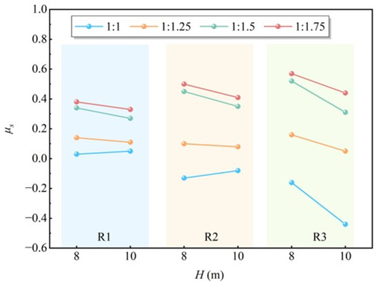
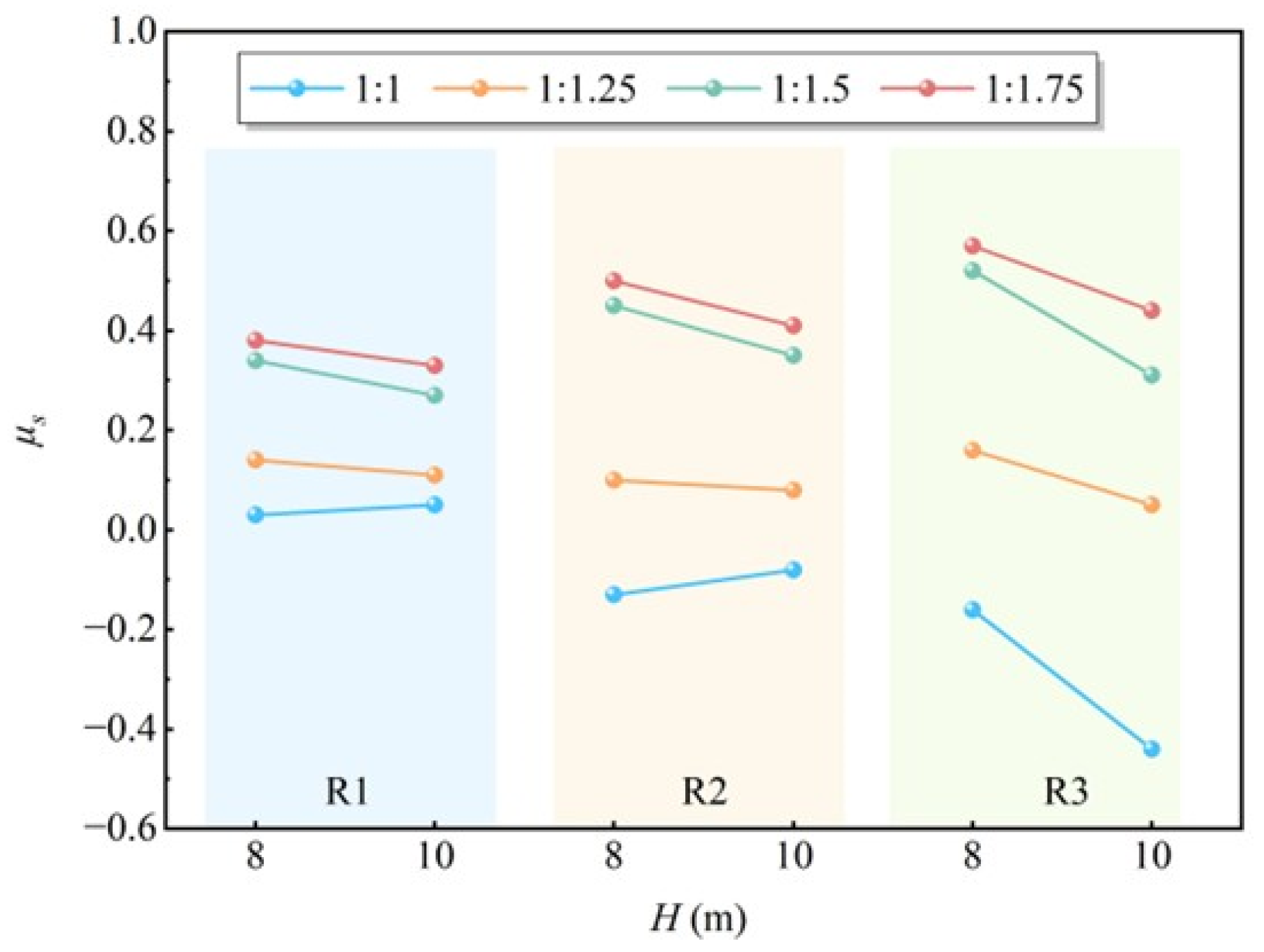
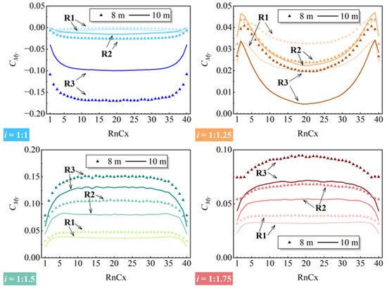
Under four slope-gradient conditions, comparative analyses of the row-wise μs and CMy of photovoltaic arrays with slope heights of 8 m and 10 m were compared, as shown in Figure 16 and Figure 17.
Figure 16.
μs of array photovoltaic (Models 8–15).
Figure 17.
CMy of array photovoltaics (Models 8–15).
Row-to-row differences in μs persist under all slope ratios, and their magnitude is generally larger than the differences caused by slope height. This indicates that, under array deployment conditions, variations in slope ratio are the primary factor controlling the spatial distribution of μs, as they dominate the wake superposition characteristics within the array. In contrast, slope height mainly produces secondary scaling effects on this distribution. In other words, the slope ratio determines the relative magnitude of μs across the array and the most unfavorable positions. Slope height, on the other hand, affects only the absolute μs for each row without altering the overall distribution pattern.
Considering the directional effect of slope height, compared with H = 8 m, μs for each row under H = 10 m show only minor adjustments, which vary depending on the slope ratio. In slope-ratio ranges corresponding to higher net wind pressure on the array, μs shifts caused by slope height are more easily discernible. In cases with inherently low μs, the curves with changing slope height tend to converge. This pattern indicates that slope height mainly influences μs by raising the crest shear layer, which in turn modifies the effective inflow experienced by the array. When the array is subjected to strong inflow and large pressure differences (determined by slope ratio), differences in effective inflow due to slope height are directly reflected in μs. In contrast, when the array is already dominated by the low-speed layer, slope height has a secondary effect.
In summary, the μs of array photovoltaics under varying slope heights primarily exhibits amplitude modulation while maintaining the overall distribution pattern. Increasing slope height does not alter the row-to-row flow differences within the array, but by shifting the position of the shear layer and the low-speed background, it produces limited adjustments to the μs of each row.
Comparing the two slope heights, the effect of slope height on CMy is mainly reflected in an overall vertical shift of the curves, while the column-wise distribution patterns and the locations of end disturbances remain largely unchanged. This indicates that slope height primarily alters the overall inflow and pressure difference environment experienced by the array, rather than changing the underlying mechanism of three-dimensional end effects.
Under steep-slope conditions (i = 1:1), all three rows exhibit negative CMy. The magnitude of the negative coefficient increases significantly from the front to the rear row. For instance, R3 has a CMy of −0.15, which is noticeably larger in magnitude than those of R2 and R1. When slope height increases from 8 m to 10 m, the curves for all three rows shift upward. For the other slope conditions, all three rows exhibit positive CMy. Increasing the slope height from 8 m to 10 m causes the curves for all rows to shift downward. These phenomena can be summarized as follows: increasing slope height generally weakens the moment effect on the photovoltaic array. This reflects that slope height modifies the relative contributions of the crest acceleration zone and the toe deceleration zone to the array moments. A higher slope moves the array farther from the slope crest, reducing the influence of the acceleration zone. As a result, the array experiences a more uniform inflow, which decreases pressure differences across the rows and leads to weaker moment effects. Correspondingly, the reduction in moment effect is most pronounced for R3. The rear-row modules are more exposed to the acceleration zone near the crest, making them more sensitive to changes in slope height compared with the front rows.
When examining the most unfavorable moment locations, the relative row-wise ranking of CMy remains consistent for both 8 m and 10 m slope heights across all four slope-ratio cases. Only in the i = 1:1 case is R1 the most critical position, but its overall magnitude is noticeably different from that of other cases. For the other three slope-ratio cases, the most unfavorable position occurs at R3, with moments decreasing sequentially from R3 to R2 to R1.
In summary, slope height can modulate the overall moment levels of the array. However, the rear-row modules consistently represent the most unfavorable positions. On gentler slopes, the rear-row modules experience positive moments, whereas on steeper slopes, they are subjected to negative moments. At the same time, the positive moment effect on the front-row modules under steep-slope conditions also warrants attention.
5. Discussion
This study aims to clarify how highway-slope topography modifies the near-ground wind environment and how such modifications translate into wind-load implications for HSPV arrays. The results reveal a consistent along-slope mechanism: toe-region deceleration in the near-ground layer, followed by an acceleration zone over the mid-to-upper slope and localized amplification near the crest, while the main flow layer remains close to the theoretical boundary-layer profile. The topographic influence becomes critical for PV systems when the disturbed near-ground layer overlaps with the typical installation height range; in such cases, both the deviation magnitude (wind-profile deviation δ) and the affected vertical extent (recovery height ZR) increase, and the topography–array coupling further produces pronounced row-to-row differentiation, with the rear rows exhibiting the most unfavorable pressure and moment responses. Physically, along-slope acceleration increases the local dynamic pressure, whereas the rapid terrain change near the crest can strengthen shear-layer development and may promote localized separation/reattachment, generating coherent vortices and associated suction zones. These vortex–wake structures interact with the module surfaces and can intensify negative pressures on the upper surface or modify under-module pressure through entrainment, leading to the observed positive/negative load patterns. Within arrays, wake shielding and vortex superposition accumulate downstream, making the rear rows more prone to amplified suction or net pressure effects under specific slope configurations. Accordingly, design-level assessments should focus on configurations that intensify the disturbed layer and treat the rear-row response as the governing condition.
Compared with previous studies on PV wind loads over flat ground [13,14,15,16,17,18,19,20,21,22], the present work focuses on highway embankment slopes where topography-induced flow modification and array wake effects coexist and interact. While recent studies have reported wind-load features for PV arrays on hillslope terrains [23,24], their configurations differ from HSPV deployments in highway slopes, where modules are typically arranged close to the slope surface with distinct array scales and layouts; thus, the aerodynamic mechanisms and load patterns may not be directly transferable. In current engineering practice, GB 50009-2012 [11] mainly accounts for terrain influence through a height-dependent wind-pressure coefficient, which does not explicitly resolve the slope-toe deceleration, crest-adjacent acceleration, or the associated topography–array coupling observed in this study. Similar simplifications are also common in practical PV design workflows referenced by GB 50797-2012 [12] and the wind-load framework of ASCE/SEI 7-10 [8]. Therefore, the present results complement the existing literature by providing mechanisms specific to highway-slope PV systems.
6. Conclusions
Through numerical simulations, a modeling approach for analyzing wind loads on HSPV systems was established. The evolution mechanisms of the wind environment over highway slopes under topographic effects were investigated, along with the influence of slope height and slope ratio on HSPV wind loads. Compared with prior hillslope PV configurations, this study focuses on highway embankment slopes and dense slope-mounted arrays, providing highway-specific evidence on topographic effects. The main conclusions are summarized as follows:
- The accuracy of the numerical model for calculating wind loads on HSPV was validated through multiple comparisons, including wind profile analysis, mesh sensitivity analysis, and wind tunnel experiments, ensuring the reliability of the simulation approach.
- The evolution of wind profiles is characterized by deviations from the theoretical exponential law. These deviations are primarily concentrated in the near-ground layer, extending from the slope toe to near the slope crest. Along the slope, the wind gradually transitions from deceleration zones to acceleration zones. The extent of topographic effects was quantified using wind profile deviation and recovery height. Larger embankment heights or steeper slopes amplify topographic effects and extend their vertical influence.
- Regarding mean wind speed characteristics, the along-wind speed ratio reveals the fundamental pattern: deceleration occurs near the slope toe, while acceleration develops over the mid-to-upper slope and crest. This pattern becomes more pronounced as the slope height and slope ratio increase. Although the crosswind and vertical wind speed ratios are relatively small, local peaks along the slope indicate noticeable uplift effects.
- Slope ratio affects the coupling of topographic and array effects, leading to more pronounced row-to-row differentiation within slope arrays. Both shape coefficients and moment coefficients exhibit the most unfavorable responses in the rear rows. This highlights that the assessment of slope-related adverse effects should focus on the rear rows, rather than relying on single-row or front-row responses.
- Slope height primarily modulates the near-field flow structure by altering the spatial scale of topographic effects. Increasing slope height raises the vertical influence of acceleration on the windward side and expands the low-speed wake region on the leeward side, stabilizing the stratified velocity structure. Variations in slope height mainly produce overall adjustments to the mechanical response of PV arrays, with the rear rows remaining the critical locations for controlling adverse moments and net wind pressures.
In engineering practice, peak effects are commonly evaluated via code-based gust factors; the mean coefficients reported here can be used as topography-induced amplification descriptors and combined with such factors for design-level checks. From a planning perspective, slope ratio should be prioritized as the primary geometric parameter to mitigate wind-load amplification, while slope height can be used for secondary refinement once a feasible slope ratio is selected. The “wind recovery capacity” can be practically interpreted by the recovery height ZR: smaller ZR indicates a thinner disturbed near-ground layer and is generally more favorable for wind-resistant design, whereas larger ZR suggests a more conservative consideration, particularly for the rear rows. Future work may extend this study in two directions. First, incorporating unsteady winds and broader wind-direction cases would better represent real roadside conditions. Second, additional field or wind-tunnel measurements for typical highway slopes, together with representative surface roughness for road asphalt and slope surfaces, could further support model calibration and strengthen the generality of the proposed findings.
Author Contributions
Conceptualization, M.S. and H.Z.; Data curation, M.S.; Formal analysis, M.S. and Z.Z.; Investigation, M.S. and H.Z.; Methodology, H.Z.; Validation, M.S. and Z.Z.; Writing—original draft, M.S. and Z.Z.; Writing—review and editing, Z.Z. All authors have read and agreed to the published version of the manuscript.
Funding
This research and the APC were funded by the National Key Research and Development Program of China, grant number 2023YFB2604600 (Energy Self-Sufficiency Technology for Intelligent Connected Road Transportation Systems).
Data Availability Statement
The original research data presented in this study are included in the article. Further inquiries can be directed to the corresponding author.
Conflicts of Interest
The authors declare no conflicts of interest.
Abbreviations
The following abbreviations are used in this manuscript:
| CFD | Computational Fluid Dynamics |
| RANS | Reynolds-Averaged Navier–Stokes |
| SST | Shear Stress Transport |
| HSPV | Highway Slope-Mounted Photovoltaic |
| PV | Photovoltaic |
References
- Pan, H.; Qi, L.; Zhang, Z.; Yan, J. Kinetic Energy Harvesting Technologies for Applications in Land Transportation: A Comprehensive Review. Appl. Energy 2021, 286, 116518. [Google Scholar] [CrossRef] [Scilit]
- Wang, L.; Wang, H.; Zhao, Q.; Yang, H.; Zhao, H.; Huang, B. Development and Prospect of Intelligent Pavement. China J. Highw. Transp. 2019, 32, 50–72. [Google Scholar] [CrossRef]
- Yang, J. Application Technology of Solar Photovoltaic Power Generation, 3rd ed.; Publishing House of Electronics Industry: Beijing, China, 2017. [Google Scholar]
- Hu, H.; Zha, X.; Lv, R.; Qiu, M.; Zhong, H.; Li, Z.; Pan, Q. Recent Advances of Energy Harvesting Technologies in Road Based on Photovoltaic Power Generation. Mater. Rep. 2022, 36, 133–144. [Google Scholar] [CrossRef]
- Poe, C.; Filosa, G. Alternative Uses of Highway Rights-of-Way: Accommodating Renewable energy technologies. Transp. Res. Rec. 2012, 2270, 23–30. [Google Scholar] [CrossRef] [Scilit]
- Jiang, H.; Cen, Y.; Zha, X.; Zhang, Q. Current Situation and Development Trend of Solar Pavement Technology. In Proceedings of the DEStech Transactions on Environment, Energy and Earth Sciences, Iași, Romania, 18–19 October 2018. [Google Scholar] [CrossRef] [Scilit]
- Meng, J.; Jia, W.; Zhang, H.; Fan, T.; He, J. ‘Solar Photovoltaic+’ Multi-Scenario Application Helps to Cope with Climate Change. China Environ. 2021, Z1, 44–47. [Google Scholar]
- ASCE/SEI 7-10; Minimum Design Loads for Buildings and other Structures. American Society of Civil Engineers: Reston, VA, USA, 2012.
- EN 1991-1-4; Eurocode 1: Actions on Structures—Part 1-4: General Actions—Wind Actions. National Annex NF EN 1991-1-4-2005/NF P06-114-1/NA/A2-2012. European Committee for Standardization (CEN): Brussels, Belgium, 2012.
- Japan Photovoltaic Energy Association. Design and Construction of Solar Photovoltaic Power Generation Systems, 4th ed.; Science Press: Beijing, China, 2013. [Google Scholar]
- GB 50009-2012; Load Code for the Design of Building Structures. Ministry of House and Urban-Rural Development of the People’s Republic of China: Beijing, China, 2012.
- GB 50797-2012; Standard for Photovoltaic Power Station. Ministry of House and Urban-Rural Development of the People’s Republic of China: Beijing, China, 2012.
- Shademan, M.; Barron, R.; Balachandar, R.; Hangan, H. Numerical Simulation of Wind Loading on Ground-Mounted Solar Panels at Different Flow Configurations. Can. J. Civ. Eng. 2014, 41, 728–738. [Google Scholar] [CrossRef] [Scilit]
- Zhang, S.; Sun, S.; Qin, L.; Shao, N. Wind Tunnel Experimental Study on Wind Load Shape Coefficients of Photovoltaic Modules. Low Carbon World 2017, 12, 89. [Google Scholar] [CrossRef]
- Chowdhury, M.; Goossens, D.; Goverde, H.; Catthoor, F. Experimentally Validated CFD Simulations Predicting Wind Effects on Photovoltaic Modules Mounted on Inclined Surfaces. Sustain. Energy Technol. Assess. 2018, 30, 201–208. [Google Scholar] [CrossRef] [Scilit]
- Abiola-Ogedengbe, A.; Hangan, H.; Siddiqui, K. Experimental Investigation of Wind Effects on a Standalone Photovoltaic (PV) Module. Renew. Energy 2015, 78, 657–665. [Google Scholar] [CrossRef] [Scilit]
- Su, K.; Chung, K.; Hsu, S. Numerical Simulation of Wind-Loaded on Solar Panels. Mod. Phys. Lett. B 2018, 32, 1840009. [Google Scholar] [CrossRef] [Scilit]
- Jiang, J.; Zhang, Z.; Lu, Y.; Zhang, T.; Zhang, J.; Li, J.; Miao, F.; Wang, Y.; Wu, K.; Zhang, D. Numerical Analysis of Wind Loads about Photovoltaic Arrays Considering Bending Moment. Renew. Energy Resour. 2019, 37, 46–52. [Google Scholar] [CrossRef]
- Chai, X. Research on Wind Loads on Flexible Solar Photovoltaic Support System. Master’s Thesis, Shijiazhuang Tiedao University, Shijiazhuang, China, 2020. [Google Scholar] [CrossRef]
- Ma, W.; Sun, G.; Liu, X.; Xing, K.; Liu, Q. Tests for Wind Load Distribution Model of Solar Panels. J. Vib. Shock 2017, 36, 8–13. [Google Scholar] [CrossRef]
- Hauf, T.; Neumann-Hauf, G. The Turbulent Wind Flow over an Embankment. Bound. Layer Meteorol. 1982, 24, 357–369. [Google Scholar] [CrossRef] [Scilit]
- Frank, H.; Heldt, K.; Emeis, S.; Fiedler, F. Flow over an Embankment: Speed-Up and Pressure Perturbation. Bound. Layer Meteorol. 1993, 63, 163–182. [Google Scholar] [CrossRef] [Scilit]
- Xu, Y.; Tian, R.; Li, B.; Jiang, F.; Hao, S. Wind Tunnel Test Study on Terrain Effect of Wind Load on Mountain Solar Panel Arrays. China Civ. Eng. J. 2026, 59, 35–46. [Google Scholar] [CrossRef]
- Zhong, W.; Zhou, Q.; Zhou, Z.; Long, H. Research on Wind Load Interference Effect of Photovoltaic Arrays under Different Hillside Terrains. J. Nat. Disasters 2023, 32, 104–112. [Google Scholar] [CrossRef]
- JTG D30-2015; Specifications for Design of Highway Subgrades. Ministry of Transport of the People’s Republic of China: Beijing, China, 2015.
- Sun, X.; Xu, W.; Wu, Y. Study on Computational Domain Setup in Bluff Body Flow. In Proceedings of the 13th National Conference on Structural Wind Engineering; Bridge and Structural Engineering Branch, China Civil Engineering Society: Beijing, China, 2018. [Google Scholar]
- Tominaga, Y.; Mochida, A.; Yoshie, R.; Kataoka, H.; Nozu, T.; Yoshikawa, M.; Shirasawa, T. AIJ Guidelines for Practical Applications of CFD to Pedestrian Wind Environment around Buildings. J. Wind Eng. Ind. Aerodyn. 2008, 96, 1749–1761. [Google Scholar] [CrossRef] [Scilit]
- Chang, F. Analysis of Wind Loads on Ground-Mounted PV Arrays with Wall Shielding. Master Thesis, Shenyang Aerospace University, Shenyang, China, 2019. [Google Scholar] [CrossRef]
- Tang, Y.; Zheng, S.; Zhao, B.; Li, M. Numerical Investigation on the Self-Sustaining of Equilibrium Atmosphere Boundary Layers. Eng. Mech. 2014, 31, 129–135. [Google Scholar] [CrossRef]

Disclaimer/Publisher’s Note: The statements, opinions and data contained in all publications are solely those of the individual author(s) and contributor(s) and not of MDPI and/or the editor(s). MDPI and/or the editor(s) disclaim responsibility for any injury to people or property resulting from any ideas, methods, instructions or products referred to in the content. |
© 2026 by the authors. Licensee MDPI, Basel, Switzerland. This article is an open access article distributed under the terms and conditions of the Creative Commons Attribution (CC BY) license.