


Abstract
Multispectral (MS) satellite imagery provides rich spectral information for surface and atmospheric interpretation, yet its spatial resolution is often limited by sensor design. In this study, we propose a Transformer-based MS super-resolution framework that uses high-resolution panchromatic (PAN) imagery to supply complementary spatial detail cues for MS reconstruction and explicitly separates spatial enhancement from spectral preservation. In the spatial branch, PAN features are aligned to the MS grid via Pixel-Unshuffle and encoded with shifted-window self-attention to capture long-range spatial dependencies efficiently. In the spectral branch, spectral self-attention treats bands as tokens to learn inter-band correlations and maintain spectral consistency. The two representations are fused through channel concatenation and a 1 × 1 convolutional module, followed by a reconstruction head that upsamples the fused features to generate high-resolution MS outputs. For training, low-resolution MS inputs are synthesized from KOMPSAT-3A MS imagery using a degradation pipeline that combines modulation transfer function-based blur, downsampling, and additive Gaussian noise; the operation order is randomly permuted to emulate diverse acquisition conditions. In addition, Bayesian optimization is employed to explore network configurations through jointly considering the normalized mean absolute error and inference time. Experiments demonstrate that the proposed approach attains 46.23 dB PSNR, 0.9735 SSIM, and 3.12 ERGAS with approximately 167.4 K parameters, achieving a high restoration quality and computational efficiency across diverse degradation settings.
1. Introduction
Low-Earth-orbit (LEO) satellites enable the frequent observation of the Earth due to their short revisit intervals, providing wide-area data for various remote sensing applications, including climate change analysis, ecosystem monitoring, crop assessment, and urban expansion tracking. In this context, satellite observation serves as a key complement to ground-based measurements by supporting continuous monitoring over large regions.
Optical Earth-observation systems are typically designed to acquire both a high-resolution single-band panchromatic (PAN) image and a multi-band multispectral (MS) image to capture spatial and spectral information simultaneously [1,2]. While MS imagery is essential for performing spectral analysis, its spatial resolution is commonly lower than that of PAN imagery because of sensor design constraints, limiting the representation of fine structures and subtle changes. This resolution gap can become a practical bottleneck in applications that require detailed structural interpretation or the analysis of fine-grained changes in land cover, urban structures, or crop conditions over time [3].
Image super-resolution (SR) has emerged as a practical approach for mitigating this limitation by reconstructing a high-resolution image from a low-resolution observation. For MS satellite imagery, SR can enhance the delineation of fine structures and reduce the adverse impact of limited resolution on downstream tasks such as object detection, boundary extraction, and change detection.
SR research has progressed from interpolation-based methods to deep learning approaches, particularly convolutional neural network (CNN) architectures such as SRCNN, VDSR, and subsequent residual- or dense-connection variants including EDSR and RDN [4,5,6,7]. These CNN-based methods have achieved substantial improvements by effectively recovering local textures and edges through stacked local convolutions and hierarchical feature extraction. However, the intrinsic locality of convolution requires long-range dependencies to be propagated across many layers, and the effective receptive field often covers only a fraction of the theoretical one, limiting global-context modeling in high-resolution reconstruction [8,9,10]. Recently, Transformer-based SR has attracted increasing attention because self-attention can directly capture long-range interactions and global context, enabling the more effective utilization of long-range dependencies in SR [11,12,13]. Alongside Transformer-based super-resolution (SR) approaches, diffusion-based SR methods employing probabilistic generative models have recently attracted scholarly attention. These methods aim to improve perceptual quality and promote reconstruction diversity by progressively denoising input signals [14,15].
Beyond supervised MS SR, recent studies conducted in the remote sensing community have explored unsupervised SR frameworks for alleviating the strong dependence on large-scale paired low-resolution (LR)–high-resolution (HR) datasets. EDIP-Net proposes an unsupervised approach for hyperspectral image SR using only LR observations and introduces a two-stage training strategy to strengthen prior-driven reconstruction capability [16]. However, this method is specifically designed for hyperspectral scenarios and differs from the formulation of our problem in terms of data configuration, as in this study we assume PAN–MS fusion to be the primary input modality.
Another major task closely related to SR is pansharpening, which aims to generate an HR–MS image at the PAN spatial resolution by fusing the spatial information from PAN with the spectral information from MS [17,18]. Traditionally, widely adopted approaches have included component substitution (CS)-based methods such as intensity–hue–saturation (IHS), principal component analysis (PCA), Gram–Schmidt and Brovey transforms, and multiresolution analysis (MRA)-based methods such as Laplacian pyramid and wavelet-based techniques [19,20,21]. Recently, pansharpening has been extended to deep learning-based approaches such as the Pansharpening Neural Network (PNN) and PanNet, which have shown improved performance in terms of spatial detail restoration and spectral preservation [22,23]. However, pansharpening suffers from inherent limitations due to the spectral response function (SRF) mismatch between panchromatic and multispectral images, as well as the differences in sensor characteristics and image signal processing (ISP) pipelines, which can lead to significant spectral distortion during the fusion process [24]. Moreover, excessively constraining spectral preservation or placing excessive emphasis on spectral correction terms may impair the injection of spatial information, resulting in diminished detail representation and increased spatial artifacts, such as blurring and ringing [25,26,27]. This fundamental trade-off between spectral fidelity and spatial sharpness imposes structural constraints on the simultaneous achievement of high spatial resolution and spectral consistency in pansharpening.
In satellite imagery, spatial cues and spectral information exhibit intrinsically different characteristics. Processing both components within a single network pathway can introduce feature interference and representational bias because the model must simultaneously accommodate heterogeneous statistical distributions. As a result, some cues may be under-represented, potentially degrading spatial fidelity and/or spectral consistency.
To address this issue, we adopt a decoupled design that processes spatial and spectral information independently from the input stage. In addition, we perform resource-aware model selection via Bayesian optimization and assess robustness under multiple realistic degradation settings.
The main contributions of this research are summarized as follows.
- A spatial–spectral decoupled Transformer SR framework tailored to satellite imagery: By explicitly considering the different characteristics of PAN-derived spatial cues and MS spectral information, we design a dual-branch network that processes the two inputs independently rather than through a shared pathway. The proposed Transformer-based framework models long-range spatial dependencies and inter-band relationships, enabling effective spatial–spectral fusion for MS SR.
- A robustness-oriented training and evaluation strategy reflecting plausible satellite image degradations: To assess performance under diverse acquisition conditions, we adopt degradation models that reflect satellite imaging characteristics, including modulation transfer function (MTF)-based blur, downsampling, and noise, and conduct training and evaluation accordingly.
- Bayesian optimization-based hyperparameter search for a quality–efficiency trade-off: We apply Bayesian optimization to explore hyperparameters and derive an efficient network configuration that considers both restoration performance and processing time.
2. Background
2.1. PAN–MS Spatial–Spectral Characteristics and Resolution Disparity
Most Earth-observation remote sensing platforms acquire MS and PAN images concurrently. Even for the same scene, PAN and MS images differ in information content and spatial resolution because of distinct sensor design objectives and acquisition mechanisms. PAN is designed to provide a high-resolution spatial structure, while MS captures spectral information; the two are often combined when spatial–spectral complementarity is required.
In general, spatial resolution, spectral resolution, and the radiative signal-to-noise ratio (SNR) are mutually constrained by system design parameters such as the amount of light received by the optical system and exposure time, so there are limitations to simultaneously maximizing spatial clarity and spectral information preservation in a single channel. In particular, as the spectral bandwidth is narrowed to increase spectral resolving, the per-pixel photon budget decreases, making it more difficult to maintain a high SNR. To compensate for this loss, systems typically require either a larger pixel footprint or a longer integration time, which can reduce the spatial resolution or degrade operational efficiency.
Therefore, many optical imaging systems adopt a dual-channel configuration to alleviate this trade-off. Specifically, the PAN channel is designed to capture fine-scale spatial structures and object boundaries with high spatial resolution, whereas the MS channels are configured to stably record band-wise radiometric responses and distinctive spectral signatures. This system-level division of roles enables the complementary exploitation of spatial and spectral information and facilitates their effective fusion in subsequent processing.
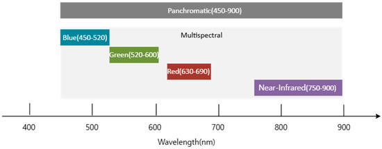
PAN imagery typically integrates a wide wavelength range spanning the visible to near-infrared spectrum into a single band, covering approximately 450–900 nm [28]. As illustrated in Figure 1, this broad spectral integration increases the photon budget per pixel, improving SNR and enabling smaller pixel sizes and, thus, a higher spatial resolution. In contrast, MS imagery uses narrower bands to capture spectral signatures, reducing the per-band photon budget and often requiring larger pixel sizes; consequently, MS images are generally provided at a coarser spatial resolution. This PAN–MS resolution disparity is commonly observed in optical remote sensing systems. Considering the characteristics and differences in resolution of optical images, in this study, we perform satellite image super-resolution under the assumption that PAN and MS images are acquired simultaneously.
Figure 1.
Wavelength ranges of PAN and MS bands.
2.2. Construction of LR–HR Pairs for SR Training
Supervised SR for satellite imagery requires spatially registered LR–HR pairs for the same scene. However, in practice, satellites do not provide native paired observations of the same scene at two spatial resolutions. Constructing LR–HR pairs through matching imagery from different satellites/sensors or acquisition times is challenging due to geometric misalignment, radiometric differences, and varying observation conditions. In particular, cross-sensor combinations often involve both radiometric discrepancies and relative geometric distortions, making it difficult to reduce registration errors in a generalized manner [29,30].
Given these constraints, supervised SR commonly synthesizes LR observations by applying degradation operators to HR imagery and uses the resulting LR–HR pairs for training. If degradation is limited to simple interpolation-based downsampling, key factors in satellite image formation, such as optical blur, detector integration/sampling, and sensor noise, are not adequately reflected. Therefore, incorporating plausible degradation factors during LR synthesis is desirable to narrow the gap between training data and real observations.
Accordingly, we construct supervised LR–HR pairs through HR-based synthetic degradation. To evaluate robustness across degradations, we validate performance under conditions that include MTF-based blur and noise.
2.3. Attention-Based Mechanism
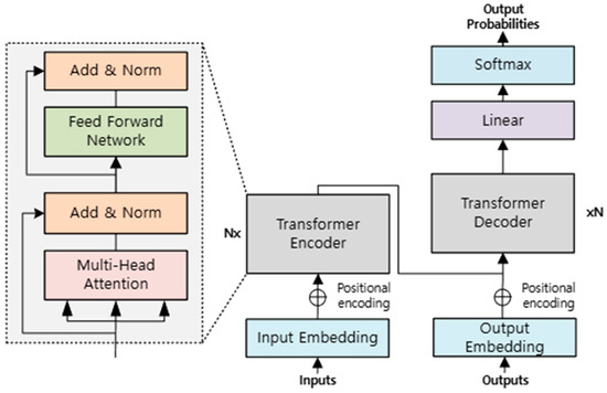
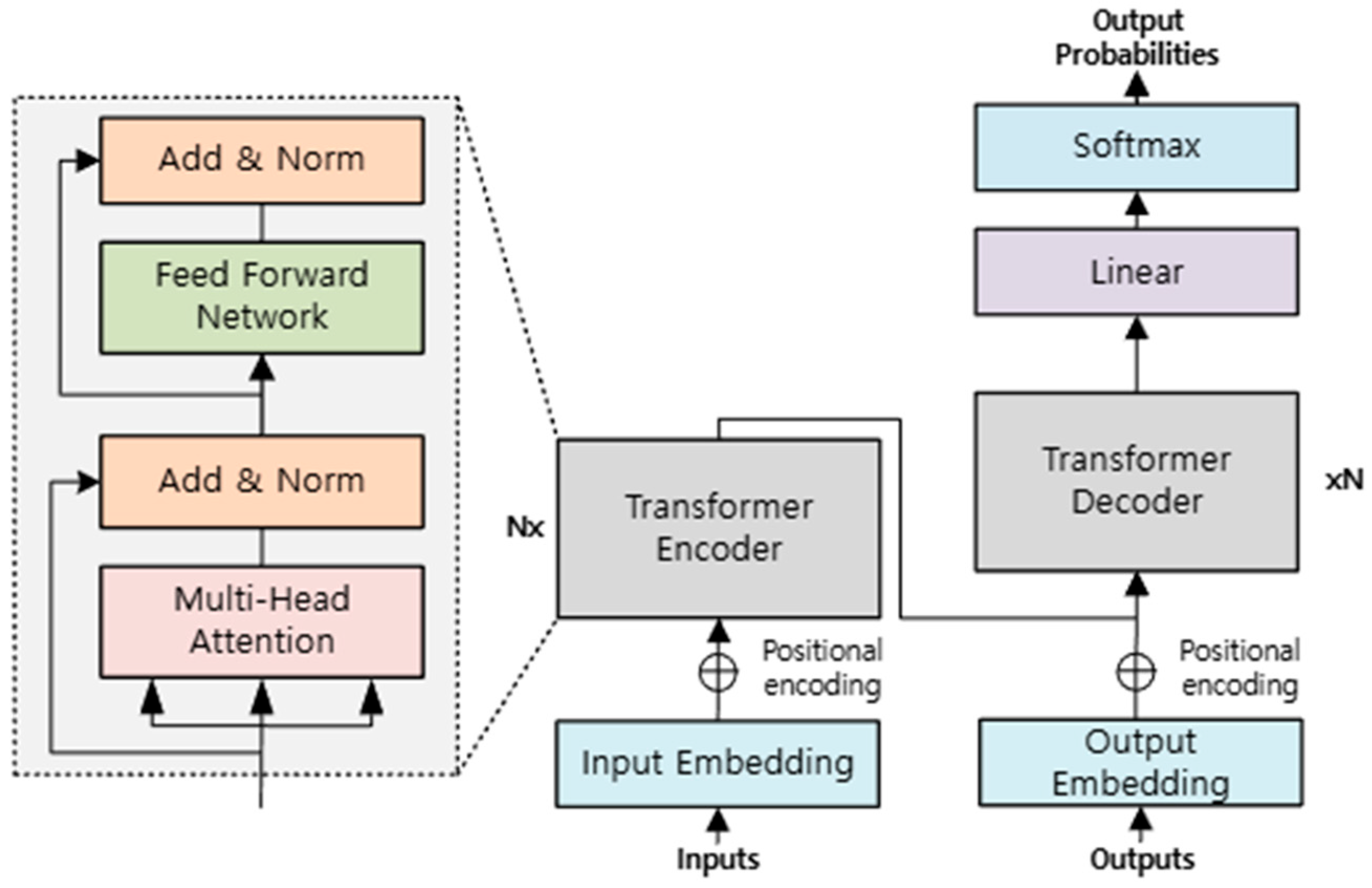
Transformers were originally introduced in natural language processing to model long-range dependencies within sequences. By learning pairwise interactions among tokens through self-attention, Transformers can represent a global context that reflects spatial relationships among features across the entire image and long-range correlations that are difficult to capture through purely local operations. Figure 2 illustrates the typical architecture of a Transformer, in which encoder and decoder blocks are stacked in layers.
Figure 2.
Transformer model architecture.
The input sequence is first projected into token embeddings, after which positional encodings are added to preserve the order information among sequence elements. The encoder consists of stacked identical blocks, each composed of a multi-head self-attention module and a position-wise Feed-Forward Network (FFN), to capture global contextual information across the entire input sequence. The decoder represents the previously generated output sequence through an output embedding layer and incorporates positional encoding to reflect the sequential order. Finally, the decoder outputs are transformed into a probability distribution over the output space through a linear projection followed by a Softmax operation. This capability motivates their adoption in low-level vision tasks where long-range spatial context is beneficial. The attention operation is formulated as shown in Equation (1):
Here, , , and denote the query, key, and value matrices projected from the input token sequence, is the number of tokens, is the key/query embedding dimension, and is applied row-wise.
In this study, the feature maps extracted from the PAN and MS branches are first converted into token sequences and then projected into the query, key, and value representations via learnable linear transformations. Here, Q, K, and V are derived from the branch-specific feature maps and are designed to capture spatial cues and spectral characteristics more effectively, respectively, thereby facilitating modality-aware attention modeling.
In our framework, the query, key, and value matrices are generated from the tokenized PAN and MS feature maps via separate learnable linear layers, where Q represents the features to be attended, and K and V encode the spatial and spectral cues that guide attention weighting.
Building on this idea, the Vision Transformer (ViT) represents an image as a sequence of patch tokens and applies self-attention, establishing a pure attention-based paradigm for visual recognition. Beyond recognition tasks, Transformer-based approaches have been actively explored for resolving low-level vision problems such as SR, denoising, and deblurring [31,32,33]. However, standard self-attention computes global interactions among all tokens, leading to quadratic computational complexity as the token count increases. To mitigate this, the Swin Transformer restricts attention to local windows and employs shifted windows to enable cross-window information exchange while maintaining computational efficiency [34].
3. Materials and Methods
3.1. Network Architecture
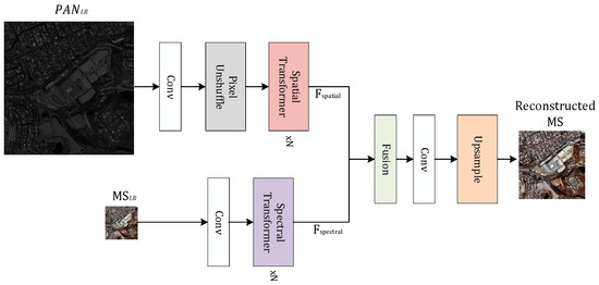
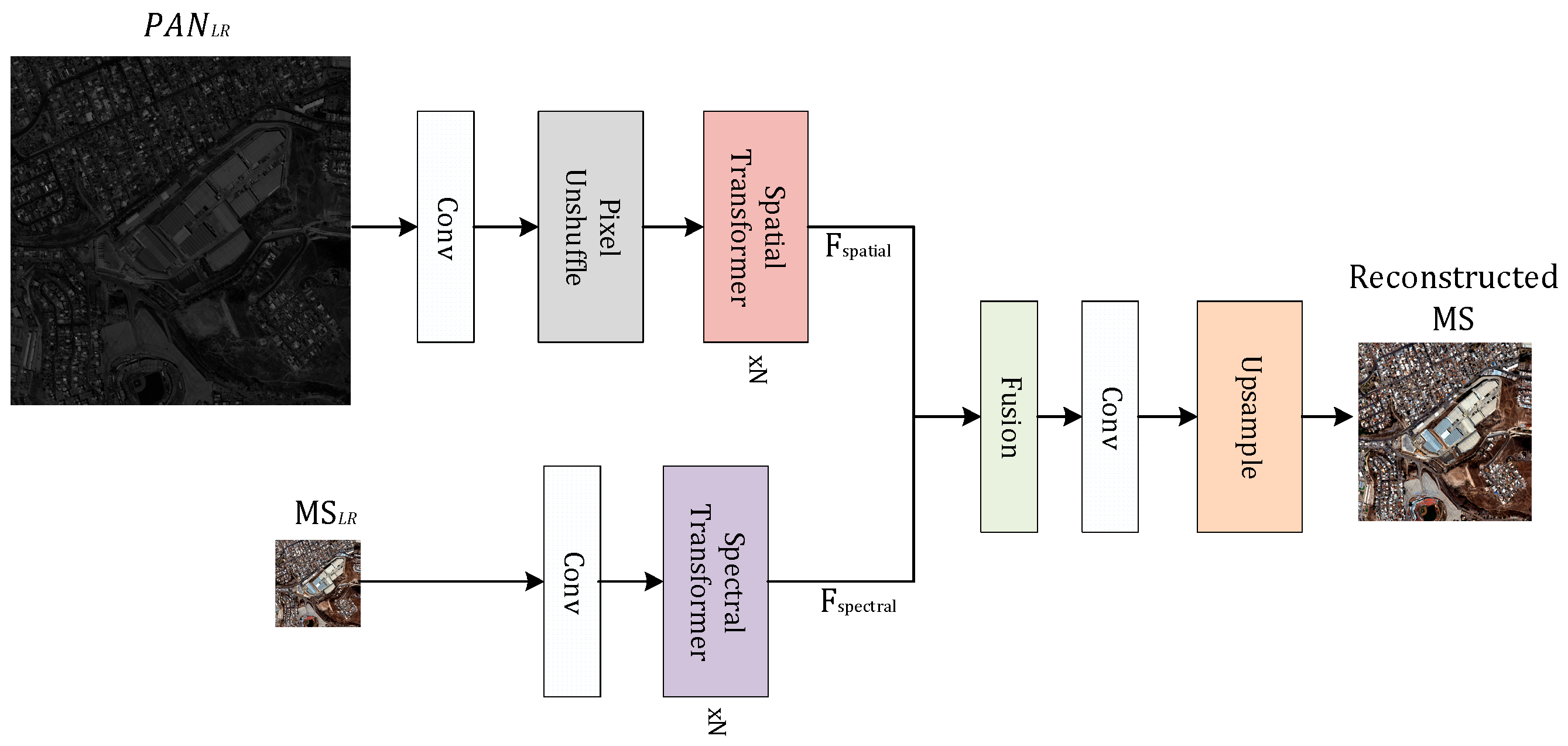
As shown in Figure 3, we proposed a dual-branch MS–SR framework that separately learns PAN-derived spatial cues and MS spectral representations and subsequently fuses them. Because PAN and MS provide complementary yet statistically different information, directly mixing them early in a single pathway can cause feature interference and bias, where spatially dominant PAN features may be disproportionately emphasized over MS features, leading the network to develop a modality-dependent learning bias toward PAN-driven cues. Dedicated feature extraction paths are, therefore, used to better exploit each modality.
Figure 3.
An overview of the proposed network architecture.
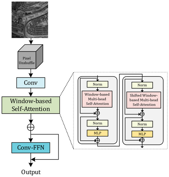
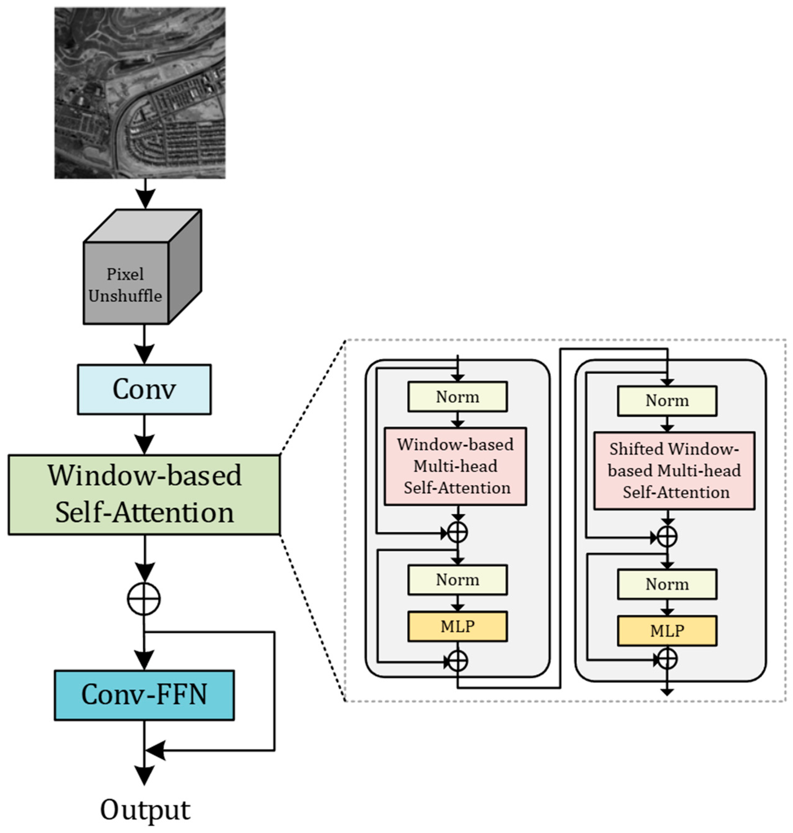
In the spatial pathway, the PAN image is first processed via convolutional layers to extract low-level features. Pixel-Unshuffle is then applied to reduce spatial resolution while increasing channel dimensionality, allowing subsequent attention blocks to operate at the MS grid with reduced cost. Window-based Transformer blocks further model local patterns and long-range spatial dependencies, effectively encoding the fine structural details present in PAN imagery.
In the spectral pathway, the MS image is encoded via convolutional layers, followed by a spectral Transformer module. By treating spectral bands as tokens and applying self-attention across bands, the module explicitly learns inter-band correlations, suppressing spectral distortion and promoting spectral consistency during SR.
The spatial and spectral features are passed to a fusion stage after resolution alignment. Convolutional fusion integrates the two representations in a complementary manner, and a reconstruction head refines the fused features and upsamples them to the target resolution. This design improves reconstruction quality while maintaining computational efficiency. Detailed module descriptions are provided in Section 3.1.1 and Section 3.1.2.
3.1.1. Spectral Branch
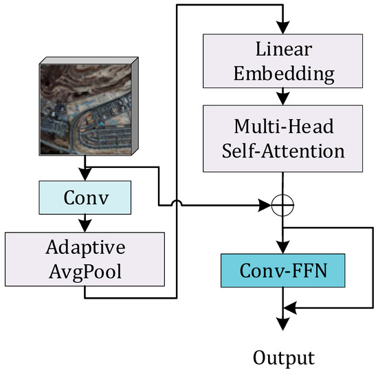
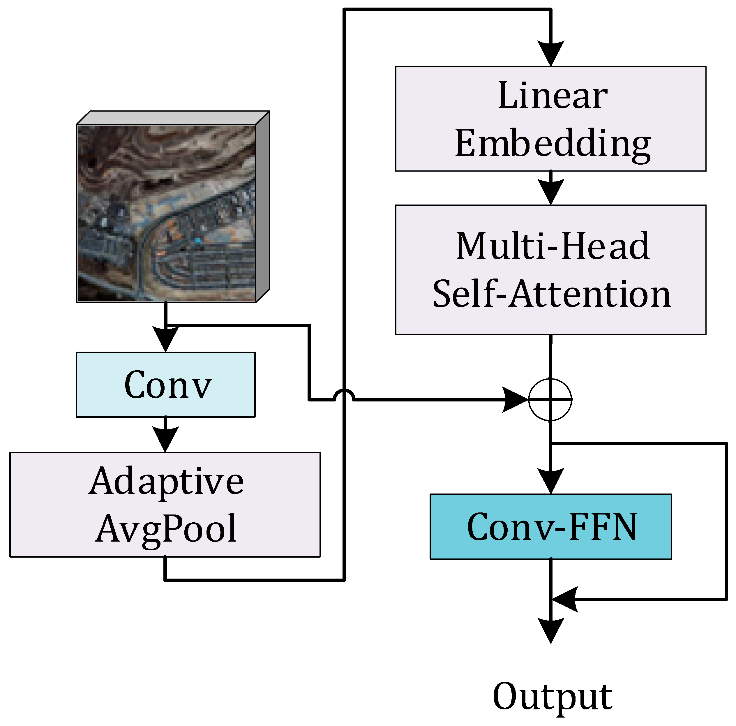
The spectral branch employs a Spectral Transformer Block to model correlations among MS bands. The block is based on spectral self-attention in which channels (bands) are treated as tokens, enabling the explicit learning of inter-band dependencies.
Specifically, given an input feature map F, adaptive average pooling is applied to obtain a global summary representation for each channel, as defined in Equation (2):
where denotes the feature value at spatial location (h,w) in the -th channel, and are the spatial height and width, is the number of channels (bands), and is the channel-wise global descriptor obtained by averaging over all spatial positions.
As depicted in Figure 4, each channel is represented as a token, and self-attention across channel tokens captures inter-band interactions and the correlation structure. The attention weights are applied to the value features, where the value features are first projected using a convolution, thereby selectively emphasizing informative channels. A convolutional FFN is further applied after attention to enhance nonlinearity and local modeling capacity. Repeating the Spectral Transformer Block at MS resolution yields meaningful spectral features while preserving spectral consistency.
Figure 4.
Spectral Transformer Block.
3.1.2. Spatial Branch
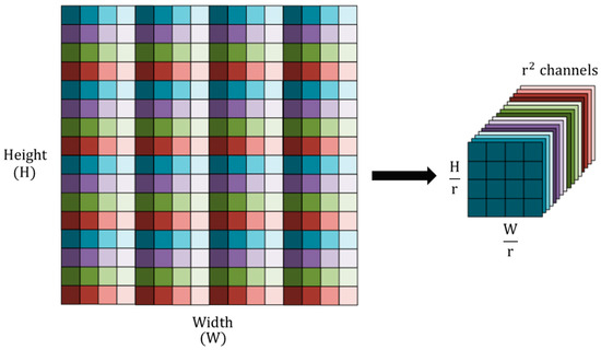
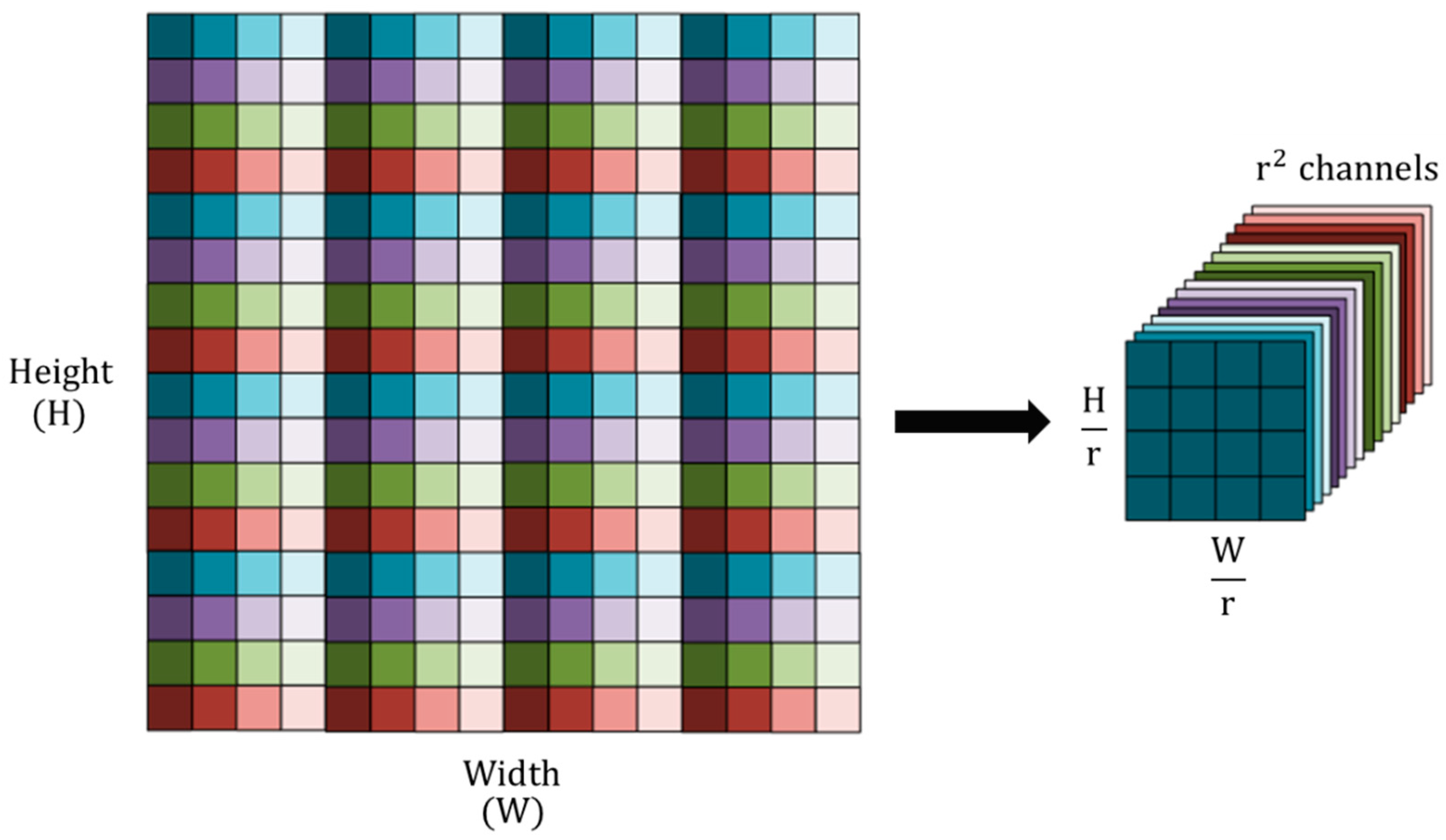
The spatial branch was designed to inject high-frequency spatial information such as edges, corners, thin linear structures, and texture transition from PAN into MS reconstruction. Since PAN and MS differ in spatial resolution, their features had to be aligned before fusion. Instead of employing naive downsampling that may have attenuated high-frequency details, we employed Pixel-Unshuffle for resolution alignment, as formulated in Equation (3):
where denotes the downscaling factor, and , , and represent the height, width, and number of channels of the input feature map.
Figure 5 illustrates the Pixel-Unshuffle operations used for resolution transformation. Specifically, Pixel-Unshuffle partitioned the input into fixed-size spatial blocks and rearranged the samples within each block into separate channel groups without any reduction operations such as averaging, interpolation, or filtering, thereby transferring sub-pixel information from the spatial domain to the channel dimension. As a result, the output was converted into a compact feature representation with reduced spatial resolution but increased channel capacity, allowing for the high-resolution structural cues of PAN to be expressed on the lower-resolution MS grid. By folding spatial information into channels, this alignment enabled parallel processing with MS features and improved computational efficiency.
Figure 5.
PAN resolution rearrangement via Pixel-Unshuffle.
The resolution-aligned PAN features were then processed via a window-based spatial Transformer module, as shown in Figure 6. Following the Swin Transformer design, attention was computed within local windows and shifted between layers to facilitate cross-window interaction. Each block included a Multi-Layer Perceptron (MLP), residual connections, and normalization to progressively refine spatial features.
Figure 6.
The Spatial Transformer Block is designed to feed MS-aligned PAN features into a window-based self-attention module for spatial detail enhancement.
3.1.3. Fusion and Reconstruction
Let the spatial and spectral features extracted from the two branches be denoted as and , with the channel dimensions and , respectively. To explicitly describe the first step of the feature fusion process, the two feature maps were first concatenated along the channel dimension, as shown in Equation (4):
where and denote the spatial and spectral feature maps, indicates channel-wise concatenation, and and are the spatial dimensions shared by the two features after Pixel-Unshuffle alignment.
The concatenated features were then fused via a convolution to mix information and reduce channels, producing a unified fused feature. This strategy was simple and computationally efficient because PAN features were already matched to the MS grid via Pixel-Unshuffle. The fused features were further refined through convolutional blocks with residual connections, and the reconstruction head upsampled the features by a factor of 2 to generate the final high-resolution multi-band MS output.
3.2. Degradation
In general, the degradation process was applied in a fixed order. An LR image was modeled as a combination of blur, downsampling, and noise applied to an HR image and can be expressed as shown in Equation (5):
where x denotes the HR image prior to degradation, * denotes convolution, k denotes the blur kernel, and (·)↓ denotes the downsampling operator with scale factor , reducing the spatial resolution by a factor of along each axis and approximating resolution loss due to sampling; moreover, n represents additive noise.
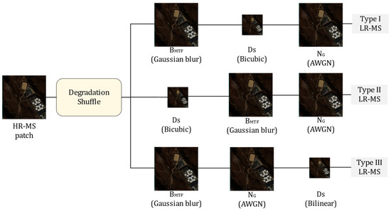
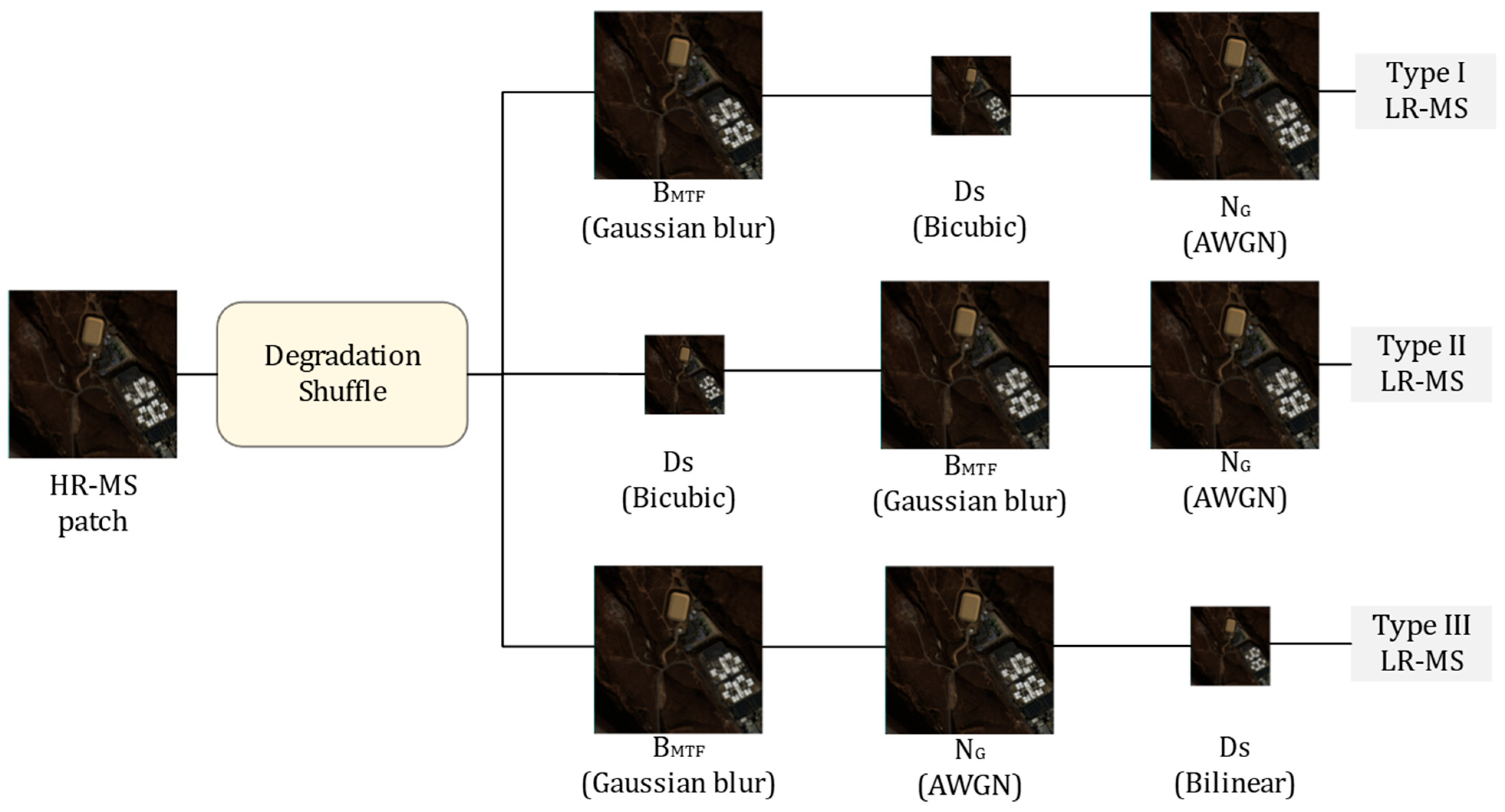
In conventional settings, degradation operations are applied in a fixed and predefined sequence. In practice, however, real satellite degradations may occur in various orders and combinations, and enforcing a fixed degradation order can induce overfitting to specific degradation patterns and hinder generalization. Accordingly, in this study, we retained the degradation components defined in Equation (5) while randomly shuffling their application order for each LR–HR pair, enabling the network to learn from diverse degradation configurations. Figure 7 illustrates the degradation pipeline applied to HR–MS patches, in which LR–HR pairs are synthesized through combinations of blur, downsampling, and noise.
Figure 7.
A degradation pipeline with a randomized operation order.
The three paths—top, middle, and bottom—depict example permutations of the degradation operations. The top path follows a conventional baseline pipeline, while the middle and bottom paths present alternative orderings. By constructing three test sets with random variations in both degradation parameters and operation order, we aimed to improve the generalization capability of the trained model.
In particular, to reflect the imaging characteristics of KOMPSAT-3A satellite data, we applied an MTF-based blur in the degradation process. The sensor spatial transfer characteristics were approximated via the frequency response process depicted in Equation (6):
where is the modulation transfer function at spatial frequency , is the standard deviation in pixels of a Gaussian used to approximate the sensor point spread function, and the estimated is used to construct a Gaussian PSF kernel so that the sensor-level attenuation of high spatial frequencies is reflected in the degradation process. The spatial frequency is expressed in cycles per pixel, and, for unit pixel sampling, the Nyquist frequency is cycles/pixel. Following the MS channel specifications of KOMPSAT-3A, the Nyquist MTF value was set to 0.13, corresponding to a standard deviation of σ = 0.64 pixels. The kernel size was then determined by truncating the Gaussian within a ±3σ range, resulting in a 5 × 5 Gaussian PSF kernel.
To simplify the modeling of sensor and quantization noise, the noise component was assumed to follow additive white Gaussian noise (AWGN). In this study, the noise mean was set to zero, and the standard deviation σ_n was fixed to 0.02 by considering the typical noise level of satellite imagery.
For downsampling, either bilinear or bicubic interpolation was randomly applied. Bilinear downsampling estimated each output pixel by linearly interpolating the values of the four nearest input samples, whereas bicubic downsampling employed a cubic interpolation kernel over a 4 × 4 neighborhood to compute each output pixel.
3.3. Hyperparameter Optimization
To derive an optimal model configuration under limited computational resources while considering both restoration accuracy and inference efficiency, we adopted Bayesian optimization to search network hyperparameters. To jointly reflect restoration quality and inference cost on the validation set, we defined the objective function for network selection as shown in Equation (7):
where w1 and w2 are weighting factors, is the normalized MAE, and is the model inference time.
In this study, to prioritize super-resolution restoration performance for satellite imagery, we assigned a relatively larger weight to the loss term and set the weighting coefficients to w1 = 0.7 and w2 = 0.3. This setting encouraged the Bayesian optimization procedure to preferentially explore configurations with superior reconstruction accuracy, while still accounting for computational efficiency to derive a balanced network configuration. However, the two terms had different units and scales, so one term may dominate the weighted sum numerically. We, therefore, applied dynamic min–max normalization to both the loss and the inference time before optimization, yielding the normalized metrics shown in Equations (8) and (9):
where denotes the -th evaluated hyperparameter configuration in the Bayesian optimization process; denotes the pixel-wise reconstruction error on the validation set; denotes the processing time measured for configuration ; and denote the minimum and maximum loss values observed up to the -th iteration, respectively; and and denote the minimum and maximum processing times observed up to the -th iteration, respectively.
After normalization, both metrics were mapped to a range between 0 and 1, which facilitated the interpretation of the weight contributions and allowed the metrics to be combined on a common scale. In addition, to mitigate the computational cost of repeated training in Bayesian optimization, the original training set was kept fixed, and a randomly sampled 10% subset was used as the validation set for objective evaluation.
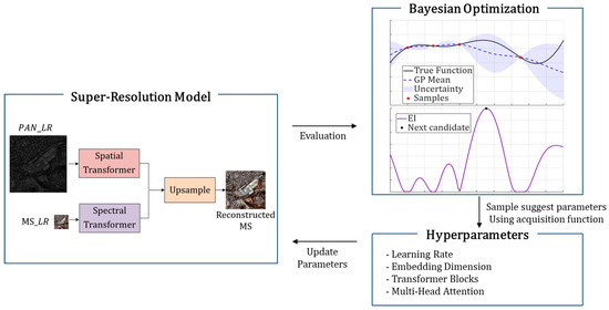
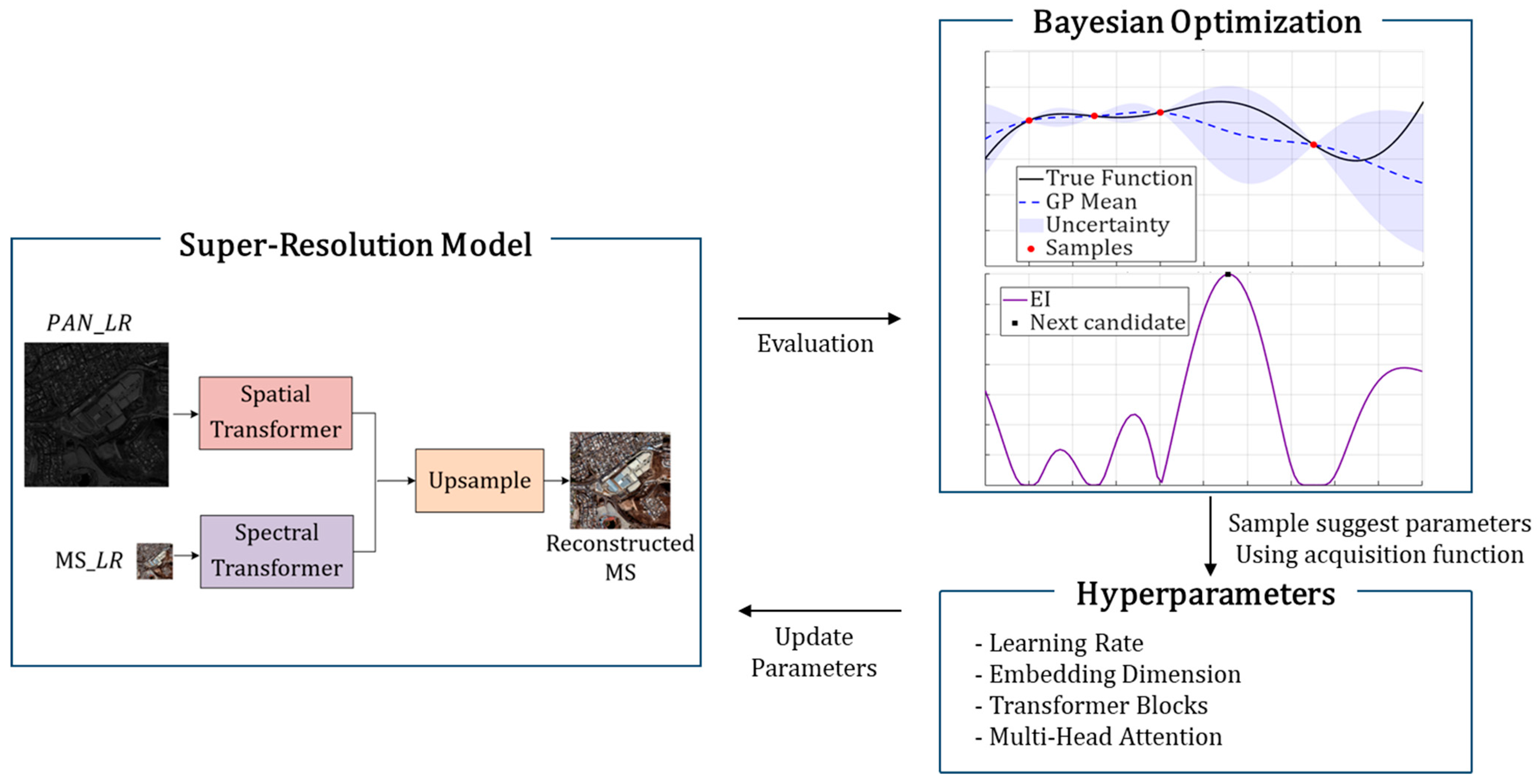
The overall Bayesian optimization procedure is schematically illustrated in Figure 8. It conceptually shows the iterative optimization loop in which the evaluation results of candidate configurations were incorporated to update the surrogate model, and a new candidate was subsequently selected based on the updated model. The search variables included structural hyperparameters such as the initial learning rate, the number of Transformer blocks, the number of attention heads, and the embedding dimension.
Figure 8.
The overall procedure for exploring optimal hyperparameters using Bayesian optimization.
The procedure consists of the initial sampling of hyperparameters, network training and validation, objective evaluation, and the selection of the next candidate based on a Gaussian process (GP) surrogate model and an acquisition function, after which the selected configuration is applied to the final SR task. In this study, we adopted a constant mean function and a radial basis function (RBF) kernel to construct the GP surrogate model, which learns from the observed hyperparameter–objective pairs and provides probabilistic predictions over the entire search space. The predictive mean and variance allow the performance landscape induced via hyperparameter variations to be approximated as a continuous stochastic process under a limited evaluation budget. To select the next candidate for evaluation, we chose the hyperparameter configuration that maximized an acquisition function computed from the GP posterior distribution. In this study, we adopted expected improvement (EI) as the acquisition function. EI is defined based on the expected improvement over the best observed objective value so far and simultaneously exploits the predictive mean μ(x) and standard deviation σ(x) of the GP posterior to balance exploitation and exploration. By considering both regions with low expected objective values and regions with high predictive uncertainty as potential candidates, this strategy enabled efficient exploration even for a limited number of trials.
In particular, jointly varying the Transformer depth and width may lead to non-uniform architecture changes, so the number of Transformer blocks is defined as a single hyperparameter and applied consistently across the network.
The search variables include both optimization-related parameters and architecture parameters, and their corresponding ranges are summarized in Table 1.
Table 1.
The hyperparameter search space for optimization.
For fair comparison across trials, all runs share the same base training settings, and only the hyperparameter configuration is updated. To avoid confounding effects due to different training budgets, we fixed the maximum training steps, as well as the evaluation, checkpointing, and logging intervals, across all trials.
3.4. Experimental
3.4.1. Dataset
The dataset used in this study is based on KOMPSAT-3A imagery. The technical specifications of the PAN and MS sensors, including their spectral bands and spatial resolutions, are summarized in Table 2. To keep input tensor dimensions consistent during mini-batch training and to control memory demand for high-resolution inputs, all scenes were tiled into fixed-size patches. Considering the trade-off between GPU memory constraints and the preservation of spatial context, PAN patches of 2048 × 2048 and MS patches of 512 × 512 were extracted. In total, 1155 patches were used for training, and 121 patches were used for testing. All experiments were conducted on a workstation equipped with an AMD Ryzen 7 9800 × 3D (8-core, 4.7 GHz) CPU, 32 GB RAM, and an NVIDIA GeForce RTX 5080 GPU (16 GB VRAM).
Table 2.
The sensor specifications for Kompsat-3A.
Training data were constructed by synthesizing LR inputs using the degradation process defined in Section 3.2. To analyze performance variation with respect to degradation settings and to avoid overfitting to a single condition, degradation models and parameters were randomly sampled to emulate diverse acquisition conditions.
For evaluation, we defined three representative degradation types to synthesize the test data, allowing for systematic assessment of model performance under diverse degradation scenarios. Specifically, for Type I, we applied bicubic downsampling via ×2 and additive noise, followed by MTF-based blur. For Type II, we applied MTF-based blur first, then bicubic ×2 downsampling and noise. For Type III, we applied noise first, then MTF-based blur, and finally bilinear downsampling.
3.4.2. Loss Function
We trained the network using a pixel-wise reconstruction loss that is widely used in SR. Specifically, we used the L1 loss as the primary training objective. Given a training set of N samples with ground truth images and corresponding network outputs, the L1 loss is defined as shown in Equation (10):
where denotes the number of training samples; denotes the ground truth image of the -th sample; denotes the corresponding network output; and denote the spatial height and width of the image; denotes the number of channels or spectral bands; , , and denote the indices of height, width, and channel, respectively; and denotes the absolute value operator.
Accordingly, the loss is computed as the mean absolute difference between the prediction and the ground truth, and the network is optimized to minimize this value during training.
3.4.3. Model Selection Through Hyperparameter Optimization
This section reports the Bayesian optimization-based hyperparameter search conducted to consider both restoration performance and inference efficiency under limited computational resources.
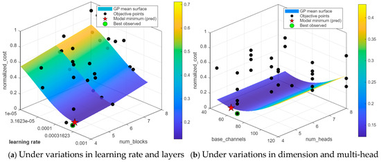
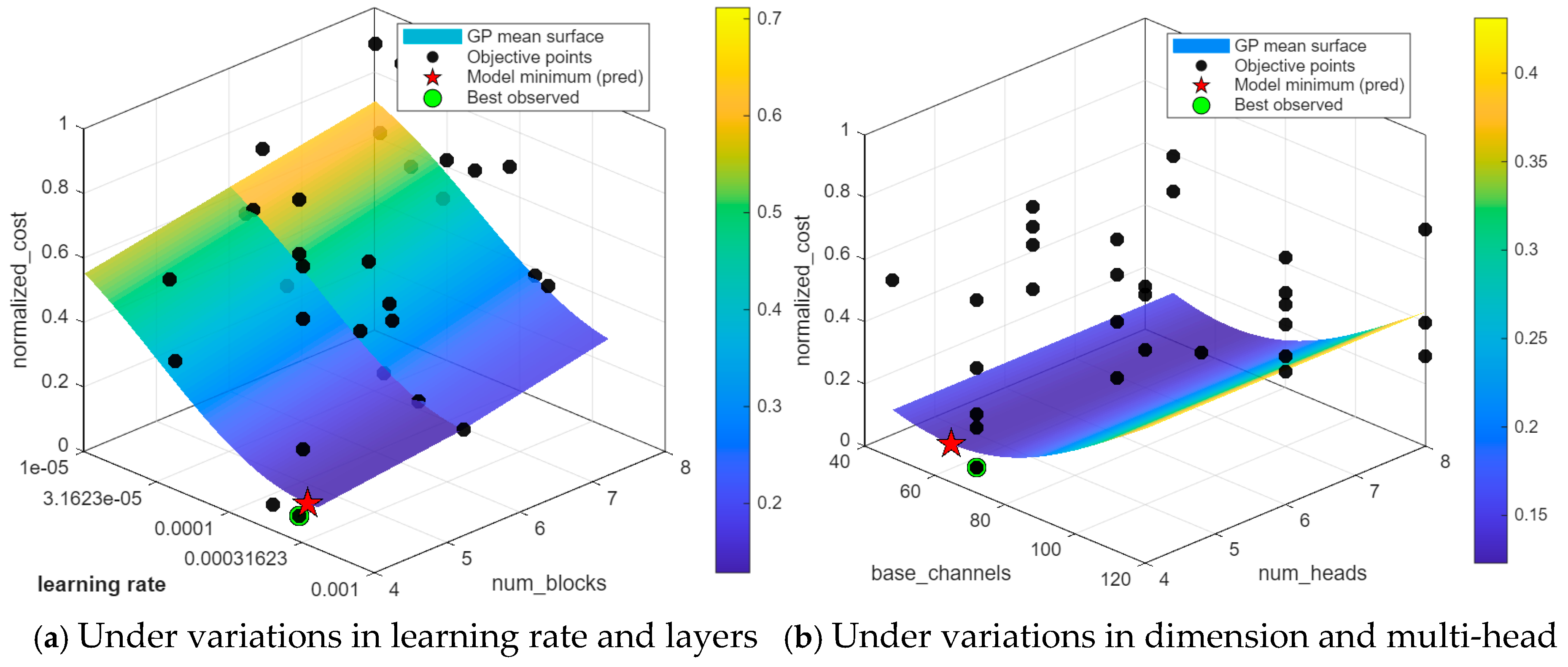
The black dots in Figure 9 represent the objective function values observed during the Bayesian optimization process under varying hyperparameter settings, while the colored surface depicts the continuous objective landscape estimated via the Gaussian process surrogate model. As shown in the figure, the objective exhibits pronounced variability with respect to the learning rate and the embedding dimension.
Figure 9.
Bayesian optimization results under hyperparameter variations.
The final network structure and hyperparameter settings are summarized in Table 3. This configuration was selected to maintain a practical balance between training stability and convergence speed through an appropriate learning rate, while suppressing the increased computational burden and latency associated with excessively scaling the number of blocks, attention heads, and embedding dimension in parallel attention operations.
Table 3.
The final hyperparameters selected via Bayesian optimization.
Table 3 summarizes the final network architecture and the selected hyperparameter settings. As the cost function used in this study jointly incorporates both the reconstruction loss and the processing time, configurations that achieve marginal accuracy gains at the expense of excessively increased latency due to a larger parameter count are penalized from an optimization perspective.
Network hyperparameters such as the embedding dimension and the number of Transformer blocks, which are included in the search space, directly determine the computational cost and parallel self-attention operations, thereby simultaneously increasing the number of model parameters and the processing time. Accordingly, a configuration that attains a low pixel-wise reconstruction error without unnecessarily increasing the parameter scale is more favorable in terms of computational efficiency under conditions of limited resources.
In other words, the proposed optimization is designed to suppress excessive growth in processing time induced via model expansion while minimizing the pixel-level reconstruction error, thereby favoring hyperparameter configurations that achieve a practical balance between performance and efficiency in lightweight architectures. As a result of this trade-off-aware Bayesian optimization, the final selected configuration contains 167K trainable parameters, representing the best balance between reconstruction performance and computational efficiency under the given constraints.
3.4.4. Evaluation Metrics
We evaluated restoration performance primarily using two widely adopted full-reference image-quality metrics, the peak signal-to-noise ratio (PSNR) and the structural similarity index (SSIM). In addition, error relative global dimensionless synthesis (ERGAS) was employed as a supplementary metric to assess the global relative reconstruction error across spectral bands.
PSNR quantifies the fidelity between the reconstructed image and the reference image and is defined as follows:
where denotes the maximum possible pixel value of the image, and denotes the mean squared error between the reconstructed image and the reference image.
In this study, was set according to 14-bit radiometric quantization. Since was computed as the average squared difference between the SR image and the HR reference, it is expressed as follows:
where and denote the height and width of the image, respectively; denotes the pixel value at location in the HR reference image; and denotes the pixel value at location in the SR reconstructed image.
PSNR is expressed in decibels (dBs) and increases as the reconstruction error decreases. SSIM measures structural similarity by considering luminance, contrast, and structural components based on the mean, standard deviation, and covariance of the two images and is defined as follows:
where and denote the reference image and the reconstructed image, respectively; and denote the mean intensities of and ; and denote the variances of and ; and denotes the covariance between and .
ERGAS is a metric that integrally evaluates the global relative reconstruction error across all spectral bands and is defined as follows:
where is the number of spectral bands, is the root mean squared error of the -th band between the SR reconstruction and the HR reference, is the mean intensity of the -th band of the reference image, and and are the spatial resolutions of the HR and LR images.
It is dimensionless, and lower values indicate a better reconstruction quality with a smaller global relative error over spectral bands.
4. Results and Discussion
4.1. Test Results
To present the reconstruction performance of the proposed model, we report results on the test datasets generated under the three degradation types defined in Section 3.4.1. In this section, the performance evaluation primarily focuses on the PSNR to measure the pixel-level fidelity between the high-resolution reference images and the reconstructed outputs. The proposed model achieves average PSNR values of 44.12 dB, 45.65 dB, and 46.23 dB under Types I–III, respectively.
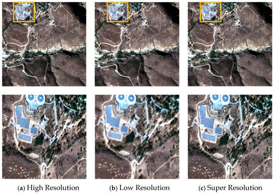
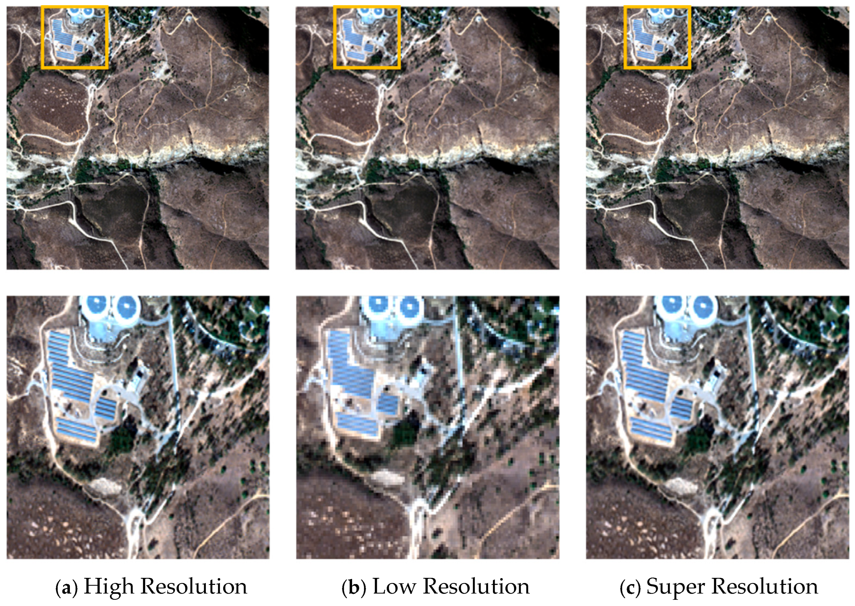
Representative qualitative examples are shown in Figure 10, which compares (a) the high-resolution reference, (b) the low-resolution input, and (c) the super-resolved output produced by the proposed method.
Figure 10.
A visual comparison of the original high-resolution MS image, the low-resolution input, and the super-resolved MS image with versions reconstructed via the proposed method.
As illustrated in the figure, the low-resolution images exhibit blurred boundaries and the loss of thin linear structures in regions characterized by prominent linear geometric patterns, such as building roofs and façades, due to degradation. The proposed model effectively recovers these degraded structural features and reconstructs MS images that closely resemble the high-resolution reference images, resulting in an improved separation of linear edges and enhanced structural continuity.
Similarly, in road–forest boundary regions, the boundary smearing and discontinuities observed in the low-resolution images are significantly reduced, and the reconstructed results exhibit the improved continuity of linear structures and sharper contours, providing a closer approximation to the boundary shapes in the high-resolution reference images. These observations indicate that the proposed model not only preserves building boundaries but also effectively suppresses degradation-induced structural losses, thereby consistently enhancing spatial resolution.
4.2. Discussion
To validate the effectiveness of the proposed model, we compare it with bicubic interpolation and representative learning-based pansharpening and SR methods, including HAN (Holistic Attention Network) and DADiff (Dual-Branch Attention-Guided Diffusion Network) [35,36]. HAN captures holistic interdependencies across layers, channels, and spatial positions using a layer attention module and a channel–spatial attention module to improve high-fidelity reconstruction. DADiff employs a diffusion branch to model the global joint distribution of PAN–MS pairs via progressive denoising, while an attention-guided branch enhances multi-scale high-frequency details; the two branches are fused to improve spatial and spectral fidelity.
For each test set constructed using randomized degradation order and parameters, we compute the mean PSNR and SSIM over all samples to quantify restoration performance. In addition, we report ERGAS to quantify the global relative reconstruction error across spectral bands.
Table 4 summarizes the quantitative performance of each method. The comparative results reveal a clear trade-off between spatial resolution enhancement and spectral fidelity among existing methods. HAN achieves a strong spatial reconstruction performance, as reflected by its high PSNR values; however, its relatively higher ERGAS indicates a limited capability in preserving spectral consistency. DADiff demonstrates improved spectral fidelity with lower ERGAS values, while achieving relatively lower PSNR in comparison with other methods. The proposed method attains SSIM values comparable to or higher than those of competing algorithms, while consistently delivering a higher PSNR. Moreover, the reduction in ERGAS indicates a decrease in the global relative reconstruction error across spectral bands, quantitatively confirming that the proposed method is not only effective at restoring spatial details but also superior in preserving spectral fidelity.
Table 4.
A performance comparison of the proposed model and existing methods.
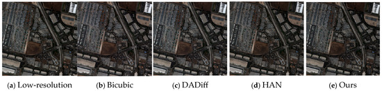
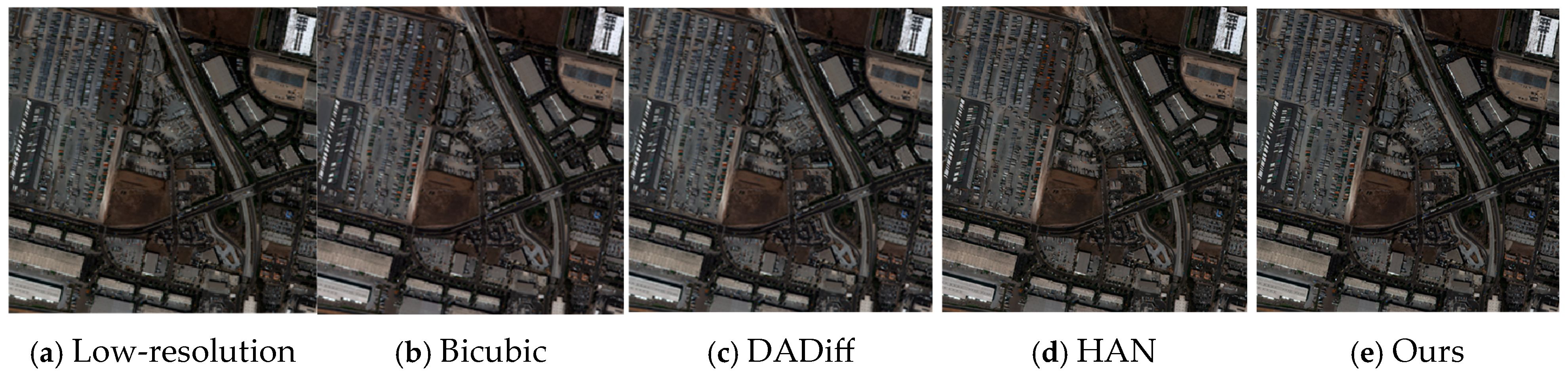
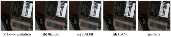
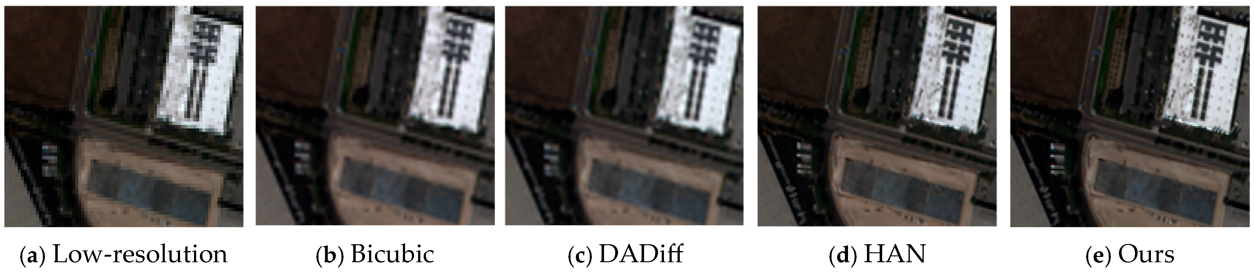
In summary, the proposed model maintains a high restoration quality while achieving favorable computational results, indicating a strong practical potential for various degradation models. Figure 11 visually compares the original image, the super-resolved results produced via the proposed model, and the corresponding low-resolution inputs. In Figure 11, bicubic interpolation produces noticeably blurred boundaries and attenuates high-frequency components, resulting in the loss of fine details in man-made structures. For a more detailed assessment, Figure 12 provides an enlarged view of the region of interest first depicted in Figure 11. The zoomed-in comparison shows that the proposed method better preserves the continuity of thin structures and reconstructs sharper edge transitions, while effectively mitigating the excessive smoothing and edge-related blurring observed in the competing approaches.
Figure 11.
A qualitative comparison of the restoration results produced via the proposed method and existing approaches.
Figure 12.
An enlarged visualization of the region of interest from Figure 11, presented for a clearer comparison.
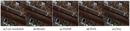
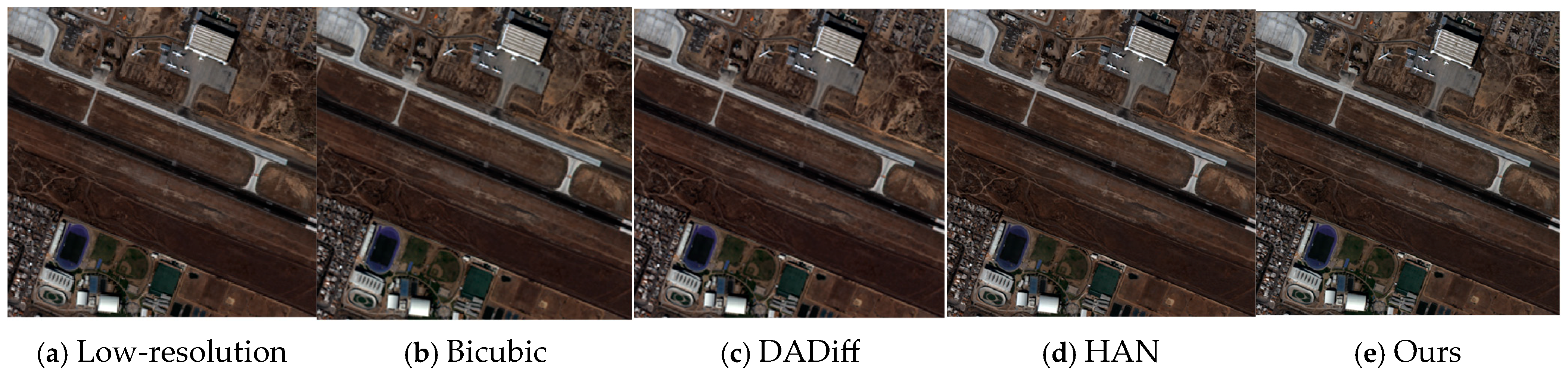
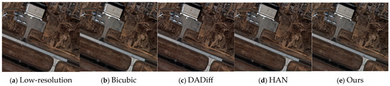
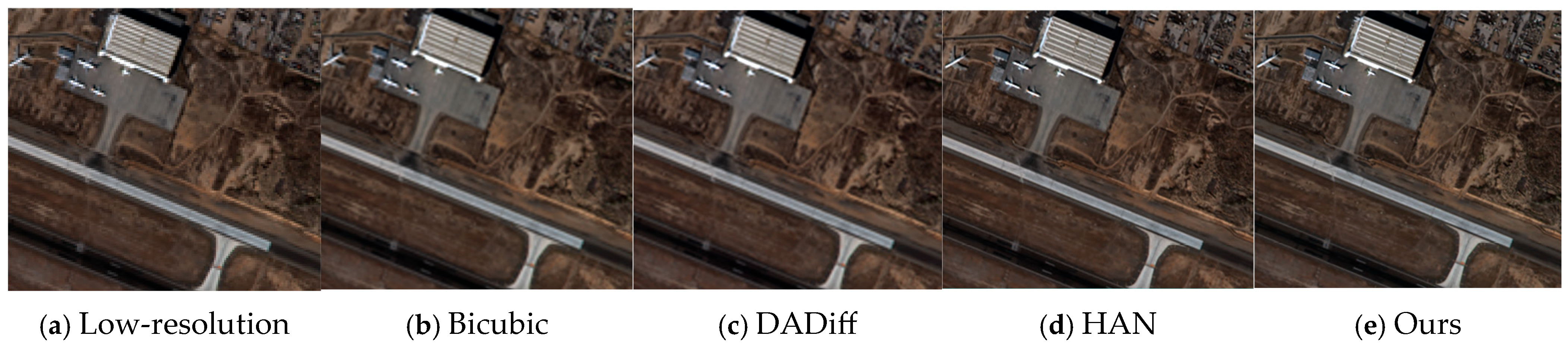
Figure 13 further evaluates the generalization capability of the proposed model for a different scenario that includes a runway and surrounding facilities. In the enlarged visualization depicted in Figure 14, the proposed method reconstructs the runway boundaries and adjacent linear structures with higher sharpness and improved structural coherence. Overall, the qualitative results in Figure 11, Figure 12, Figure 13 and Figure 14 corroborate that the proposed approach achieves a robust and favorable balance for detail restoration across diverse regions and degradation types.
Figure 13.
The region of interest selected for evaluation, showing an area that includes the runway and surrounding facilities in the remote sensing imagery.
Figure 14.
An enlarged view of the region of interest from Figure 13, depicted for a more detailed inspection of fine structures and local details.
Overall, by decoupling the high-frequency spatial information from PAN and the spectral information from MS, the proposed model can simultaneously enhance spatial sharpness and preserve spectral consistency. These results indicate that the model more effectively maintains structural consistency under degraded conditions while, at the same time, restoring high-frequency details with improved fidelity. In addition, through training and evaluation under degradation uncertainties that may arise from diverse acquisition conditions, the proposed model exhibits relatively small performance variations across degradation types and consistently maintains strong quantitative metrics, demonstrating a robust generalization capability under diverse degradation scenarios. Furthermore, by employing Bayesian optimization to jointly consider reconstruction performance and processing time, the framework enables the efficient exploration of hyperparameters, achieving not only a high reconstruction accuracy but also an effective balance between performance and computational efficiency.
Despite these advantages, several limitations remain. The present framework is not directly applicable to scenarios in which the PAN channel is unavailable, which necessitates future research on developing network designs that can operate using only a single input image. Further validation across diverse sensors and scale factors is required to establish broader generality.
5. Conclusions
In this study, we proposed a Transformer-based framework for super-resolving LEO MS satellite imagery through learning and fusing PAN-guided spatial cues and MS spectral information through decoupled branches. The PAN branch employs Pixel-Unshuffle-based alignment and window/shifted-window self-attention to preserve high-frequency structural information while controlling computational complexity. The MS branch adopts band-token spectral self-attention to explicitly model inter-band correlations and maintain spectral consistency. Robustness to acquisition variability was examined using synthetic degradations that combine MTF-based blur, downsampling, and noise with randomized operation ordering. In addition, Bayesian optimization was performed using an objective that jointly considers normalized MAE and inference time to derive a practically efficient network configuration. The experimental results show that, on the test set, the proposed method achieves average PSNR/SSIM/ERGAS values of 44.12 dB/0.9642/3.59 (Type I), 45.65 dB/0.9669/3.45 (Type II), and 46.23 dB/0.9735/3.12 (Type III) for the three degradation types, respectively. The proposed approach consistently outperforms bicubic interpolation and achieves an improved reconstruction performance compared with competing methods. In particular, under the Type III condition, our method yields PSNR gains of 0.72 dB over HAN and 3.27 dB over DADiff, while recording the lowest ERGAS among all compared approaches.
Future research can be extended in several directions. The current validation is limited to two scale factors, and further systematic evaluation across diverse satellite sensors and multiple scale factors is required to strengthen generality. In practical remote sensing operations, differences in sensor configurations, acquisition conditions, and data policies may result in scenarios where the PAN channel cannot be reliably used. To address this limitation, future studies may explore super-resolution network designs that operate on a single low-resolution MS image, as well as pretraining and domain-adaptation strategies that leverage external high-resolution remote sensing datasets. Such extensions would enable the development of a more general super-resolution framework applicable under diverse sensor configurations and data availability conditions.
Author Contributions
Conceptualization, D.Y. and S.-T.Y.; methodology, S.-T.Y.; software, D.Y.; validation, D.Y.; writing—original draft preparation, D.Y.; writing—review and editing, S.-T.Y.; visualization, D.Y.; supervision, S.-T.Y. All authors have read and agreed to the published version of the manuscript.
Funding
This research was supported by Research Resurgence under the Glocal University 30 Project at Gyeongsang National University in 2024.
Institutional Review Board Statement
Not applicable.
Informed Consent Statement
Not applicable.
Data Availability Statement
The data presented in this study are available on request from the corresponding author. The data are not publicly available due to privacy.
Conflicts of Interest
The authors declare no conflicts of interest.
Abbreviations
The following abbreviations are used in this manuscript:
| MS | Multispectral |
| PAN | Panchromatic |
| SR | Super-Resolution |
| CNN | Convolutional Neural Network |
| LEO | Low Earth Orbit |
| ViT | Vision Transformer |
| SNR | Signal-to-Noise Ratio |
| PSF | Point Spread Function |
| MTF | Modulation Transfer Function |
| AWGN | Additive White Gaussian Noise |
| FFN | Feed-Forward Network |
| PSNR | Peak Signal-to-Noise Ratio |
| SSIM | Structural Similarity Index |
| MAE | Mean Absolute Error |
| GP | Gaussian Process |
References
- Pohl, C.; van Genderen, J.L. Multisensor image fusion in remote sensing: Concepts, methods and applications. Int. J. Remote Sens. 1998, 19, 823–854. [Google Scholar] [CrossRef] [Scilit]
- Meng, X.; Shen, H.; Li, H.; Zhang, L.; Fu, R. Review of the pansharpening methods for remote sensing images based on the idea of meta-analysis: Practical discussion and challenges. Inf. Fusion 2019, 46, 102–113. [Google Scholar] [CrossRef] [Scilit]
- Munechika, C.K.; Warnick, J.S.; Salvaggio, C.; Schott, J.R. Resolution enhancement of multispectral image data to improve classification accuracy. Photogramm. Eng. Remote Sens. 1993, 59, 67–72. [Google Scholar]
- Dong, C.; Loy, C.C.; He, K.; Tang, X. Image Super-Resolution Using Deep Convolutional Networks. IEEE Trans. Pattern Anal. Mach. Intell. 2016, 38, 295–307. [Google Scholar] [CrossRef] [Scilit]
- Kim, J.; Lee, J.K.; Lee, K.M. Accurate Image Super-Resolution Using Very Deep Convolutional Networks. In Proceedings of the IEEE Conference on Computer Vision and Pattern Recognition (CVPR), Las Vegas, NV, USA, 27–30 June 2016. [Google Scholar]
- Lim, B.; Son, S.; Kim, H.; Nah, S.; Lee, K.M. Enhanced Deep Residual Networks for Single Image Super-Resolution. In Proceedings of the IEEE Conference on Computer Vision and Pattern Recognition Workshops (CVPRW), Honolulu, HI, USA, 21–26 July 2017. [Google Scholar]
- Zhang, Y.; Tian, Y.; Kong, Y.; Zhong, B.; Fu, Y. Residual Dense Network for Image Super-Resolution. In Proceedings of the IEEE/CVF Conference on Computer Vision and Pattern Recognition (CVPR), Salt Lake City, UT, USA, 18–23 June 2018. [Google Scholar]
- Luo, W.; Li, Y.; Urtasun, R.; Zemel, R.S. Understanding the Effective Receptive Field in Deep Convolutional Neural Networks. Adv. Neural Inf. Process. Syst. (NeurIPS) 2016, 29, 4898–4906. [Google Scholar]
- Zhang, Y.; Li, K.; Li, K.; Wang, L.; Zhong, B.; Fu, Y. Image Super-Resolution Using Very Deep Residual Channel Attention Networks. In Proceedings of the European Conference on Computer Vision (ECCV), Munich, Germany, 8–14 September 2018; Lecture Notes in Computer Science; Springer: Cham, Switzerland, 2018; Volume 11211, pp. 294–310. [Google Scholar] [CrossRef] [Scilit]
- Mei, Y.; Fan, Y.; Zhou, Y.; Huang, L.; Huang, T.S.; Shi, H. Image Super-Resolution With Cross-Scale Non-Local Attention and Exhaustive Self-Exemplars Mining. In Proceedings of the IEEE/CVF Conference on Computer Vision and Pattern Recognition (CVPR), Seattle, WA, USA, 13–19 June 2020; pp. 5689–5698. [Google Scholar] [CrossRef] [Scilit]
- Chen, H.; Wang, Y.; Guo, T.; Xu, C.; Deng, Y.; Liu, Z.; Ma, S.; Xu, C.; Gao, W. Pre-trained image processing transformer. In Proceedings of the IEEE Conference on Computer Vision and Pattern Recognition (CVPR), Nashville, TN, USA, 20–25 June 2021; pp. 12299–12310. [Google Scholar] [CrossRef] [Scilit]
- Liang, J.; Cao, J.; Sun, G.; Zhang, K.; Van Gool, L.; Timofte, R. SwinIR: Image restoration using Swin Transformer. In Proceedings of the IEEE International Conference on Computer Vision Workshops (ICCVW), Montreal, QC, Canada, 11–17 October 2021; pp. 1833–1844. [Google Scholar]
- Chen, X.; Wang, X.; Zhou, J.; Qiao, Y.; Dong, C. Activating more pixels in image super-resolution transformer. In Proceedings of the IEEE Conference on Computer Vision and Pattern Recognition (CVPR), Vancouver, BC, Canada, 18–22 June 2023; pp. 22367–22377. [Google Scholar]
- Zhu, C.; Liu, Y.; Huang, S.; Wang, F. Taming a Diffusion Model to Revitalize Remote Sensing Image Super-Resolution. Remote Sens. 2025, 17, 1348. [Google Scholar] [CrossRef] [Scilit]
- Lu, L.; Huang, Z.; Bao, Y.; Wan, L.; Li, Z. Multi-level Priors-Guided Diffusion-based Remote Sensing Image Super-Resolution. ISPRS J. Photogramm. Remote Sens. 2025, 228, 756–770. [Google Scholar] [CrossRef] [Scilit]
- Li, J.; Zheng, K.; Gao, L.; Han, Z.; Li, Z.; Chanussot, J. Enhanced Deep Image Prior for Unsupervised Hyperspectral Image Super-Resolution. IEEE Trans. Geosci. Remote Sens. 2025, 63, 5504218. [Google Scholar] [CrossRef] [Scilit]
- Duran, J.; Buades, A.; Coll, B.; Sbert, C.; Blanchet, G. A survey of pansharpening methods with a new band-decoupled variational model. ISPRS J. Photogramm. Remote Sens. 2017, 125, 78–105. [Google Scholar] [CrossRef] [Scilit]
- Zhou, H.; Liu, Q.; Wang, Y. PanFormer: A Transformer Based Model for Pan-Sharpening. In Proceedings of the 2022 IEEE International Conference on Multimedia and Expo (ICME), Taipei, Taiwan, 18–22 July 2022; pp. 1–6. [Google Scholar] [CrossRef] [Scilit]
- Loncan, L.; de Almeida, L.B.; Bioucas-Dias, J.M.; Briottet, X.; Chanussot, J.; Dobigeon, N.; Fabre, S.; Liao, W.; Licciardi, G.A.; Simoes, M.; et al. Hyperspectral Pansharpening: A Review. IEEE Geosci. Remote Sens. Mag. 2015, 3, 27–46. [Google Scholar] [CrossRef] [Scilit]
- Nunez, J.; Otazu, X.; Fors, O.; Prades, A.; Pala, V.; Arbiol, R. Multiresolution-based image fusion with additive wavelet decomposition. IEEE Trans. Geosci. Remote Sens. 1999, 37, 1204–1211. [Google Scholar] [CrossRef] [Scilit]
- Chavez, P.S.; Sides, S.C.; Anderson, J.A. Comparison of three different methods to merge multiresolution and multispectral data: TM & SPOT pan. Photogramm. Eng. Remote Sens. 1991, 57, 295–303. [Google Scholar]
- Yang, J.; Fu, X.; Hu, Y.; Huang, Y.; Ding, X.; Paisley, J. PanNet: A deep network architecture for pan-sharpening. In Proceedings of the IEEE International Conference on Computer Vision (ICCV), Venice, Italy, 22–29 October 2017; pp. 5449–5457. [Google Scholar]
- Masi, G.; Cozzolino, D.; Verdoliva, L.; Scarpa, G. Pansharpening by Convolutional Neural Networks. Remote Sens. 2016, 8, 594. [Google Scholar] [CrossRef] [Scilit]
- Wang, W.; Liu, H.; Xie, G. Pansharpening of WorldView-2 Data via Graph Regularized Sparse Coding and Adaptive Coupled Dictionary. Sensors 2021, 21, 3586. [Google Scholar] [CrossRef] [Scilit]
- Thomas, C.; Ranchin, T.; Wald, L.; Chanussot, J. Synthesis of Multispectral Images to High Spatial Resolution: A Critical Review of Fusion Methods Based on Remote Sensing Physics. IEEE Trans. Geosci. Remote Sens. 2008, 46, 1301–1312. [Google Scholar] [CrossRef] [Scilit]
- Vivone, G.; Alparone, L.; Chanussot, J.; Mura, M.D.; Garzelli, A.; Licciardi, G.A.; Restaino, R.; Wald, L. A Critical Comparison Among Pansharpening Algorithms. IEEE Trans. Geosci. Remote Sens. 2015, 53, 2565–2586. [Google Scholar] [CrossRef] [Scilit]
- Tsukamoto, N.; Sugaya, Y.; Omachi, S. Spectrum Correction Using Modeled Panchromatic Image for Pansharpening. J. Imaging 2020, 6, 20. [Google Scholar] [CrossRef] [Scilit] [PubMed] [PubMed Central]
- Wang, L.; Sousa, W.P.; Gong, P. Comparison of IKONOS and QuickBird images for mapping mangrove species on the Caribbean coast of Panama. Remote Sens. Environ. 2004, 91, 432–440. [Google Scholar] [CrossRef] [Scilit]
- Shi, L.; Zhao, R.; Pan, B.; Zou, Z.; Shi, Z. Unsupervised multimodal remote sensing image registration via domain adaptation. IEEE Trans. Geosci. Remote Sens. 2023, 61, 5626211. [Google Scholar] [CrossRef] [Scilit]
- Yang, K.; Li, G.; Cheng, Y. Remote sensing image registration using multiple image features and local linear transformations. Remote Sens. 2017, 9, 581. [Google Scholar] [CrossRef] [Scilit]
- Han, K.; Wang, Y.; Chen, H.; Chen, X.; Guo, J.; Liu, Z.; Tang, Y.; Xiao, A.; Xu, C.; Xu, Y.; et al. A survey on vision transformer. IEEE Trans. Pattern Anal. Mach. Intell. 2023, 45, 87–110. [Google Scholar] [CrossRef] [Scilit]
- Wang, Z.; Cun, X.; Bao, J.; Zhou, W.; Liu, J.; Li, H. Uformer: A general U-shaped transformer for image restoration. In Proceedings of the IEEE Conference on Computer Vision and Pattern Recognition (CVPR), New Orleans, LA, USA, 19–24 June 2022; pp. 17662–17672. [Google Scholar] [CrossRef] [Scilit]
- Liu, Z.; Lin, Y.; Cao, Y.; Hu, H.; Wei, Y.; Zhang, Z.; Lin, S.; Guo, B. Swin Transformer: Hierarchical Vision Transformer Using Shifted Windows. In Proceedings of the IEEE/CVF International Conference on Computer Vision (ICCV), Montreal, QC, Canada, 11–17 October 2021; pp. 10012–10022. [Google Scholar] [CrossRef] [Scilit]
- Zamir, S.W.; Arora, A.; Khan, S.; Hayat, M.; Khan, F.S.; Yang, M.-H. Restormer: Efficient transformer for high-resolution image restoration. In Proceedings of the IEEE Conference on Computer Vision and Pattern Recognition (CVPR), New Orleans, LA, USA, 19–24 June 2022; pp. 5718–5729. [Google Scholar] [CrossRef] [Scilit]
- Niu, B.; Wen, W.; Ren, W.; Zhang, X.; Yang, L.; Wang, S.; Zhang, K.; Cao, X.; Shen, H. Single Image Super-Resolution via a Holistic Attention Network. In Computer Vision—ECCV 2020; Lecture Notes in Computer Science; Springer: Berlin/Heidelberg, Germany, 2020; Volume 12357, pp. 191–207. [Google Scholar]
- Zheng, H.; Pan, C.; Jin, X.; Wozniak, M.; Wang, P.; Lee, S.-J.; Jiang, Q. A pan-sharpening model using dual-branch attention-guided diffusion networks. Inf. Fusion 2025, 120, 103076. [Google Scholar] [CrossRef] [Scilit]

Disclaimer/Publisher’s Note: The statements, opinions and data contained in all publications are solely those of the individual author(s) and contributor(s) and not of MDPI and/or the editor(s). MDPI and/or the editor(s) disclaim responsibility for any injury to people or property resulting from any ideas, methods, instructions or products referred to in the content. |
© 2026 by the authors. Licensee MDPI, Basel, Switzerland. This article is an open access article distributed under the terms and conditions of the Creative Commons Attribution (CC BY) license.