Lifespan Estimation of Closed-Circuit Television (CCTV) Systems Using Weibull Modeling

Abstract

Ensuring the availability and reliability of electronic components or materials during operation necessitates conducting a sampling inspection of their lifespan. This is particularly crucial when comparing equipment or materials deployed in various areas with diverse environments, conditions, and situations. Many studies rely on one-method parameter estimation methods, which fall short in identifying the two explicit parameters of the Weibull distribution. Moreover, inaccurate parameter estimation methods impede the attainment of reliable analysis results. Consequently, this paper introduces three analytical estimation methods to determine the parameters of the Weibull distribution. The accuracy of these methods is evaluated using the mean square error (MSE). Furthermore, we utlized the Kolmogorov–Smirnov and Anderson–Darling test on real datasets, confirming that the data follow a Weibull distribution. Simulation results indicate that the maximum likelihood estimate outperforms the other estimators by minimizing the MSE and yielding optimal parameters. These optimal parameters were then applied to real CCTV datasets, demonstrating a good fit and enabling assessment of CCTV lifespan through the mean time to failure, which is estimated to be 6.6 years. This holds true even when the equipment operates in environments with different conditions and situations.

1. Introduction

Technology systems procured by the public sector in Thailand are used to control and monitor various situations. However, these systems require an effective maintenance plan. These technologies must often involve devices equipped with electronic circuit boards. One such system is closed-circuit television (CCTV), which is used for monitoring and control in diverse scenarios, including transportation, property crime prevention, office spaces, and emergency responses. When such electronic devices are unavailable, the capacity to collect and use data for effective control and monitoring is compromised. Therefore, the public sector fails to implement appropriate maintenance policies, and a significant amount of capital may be expended annually.

The public sector must establish maintenance plans or guidelines that address the operational aspects of electronic devices and ensure reliable operation throughout their lifespan, even under conditional failures.

In this study, we focus on estimating the lifespan and reliability of CCTV systems operating in real-world environments, such as congested areas and under-building installations. Although various methods are available for lifespan evaluation, relying on a single approach to estimate Weibull parameters is insufficient. This limitation becomes critical when measurement accuracy is low and may lead to substantial estimation errors.

Additionally, simulation-based approaches can support exploration of a wider range of operating scenarios and system variations. Therefore, a comprehensive approach is required, one that considers multiple estimation methods and ensures accuracy in parameter identification within the Weibull distribution. Our contributions through this study, which evaluates the lifespan and reliability of outdoor CCTV systems, are summarized as follows:

• We utilize statistics in reliability analysis to evaluate the behavior of a CCTV system. Reliability refers to the ability of these items to perform their intended tasks without failure and within specified performance limits throughout their lifecycle [1]. This paper focuses on outdoor CCTV systems and emphasizes accurate parameter estimation using the Weibull distribution.
• To determine the lifespan of electronic devices and components, probability distributions are commonly applied. These models usually assume that items operate under uniform conditions. In practice, parameters such as the mean, standard deviation, shape, or scale often need adjustment [2]. A key aspect of this study is comparing the actual lifespan of CCTV systems in real-world environments (for example, congested areas or under-building installations) with the lifespan claimed by manufacturers. This comparison highlights discrepancies between theoretical performance and field reliability.
• To capture these real-world effects, we adjust the parameters of the Weibull distribution to reflect the operating conditions of CCTV systems. By modifying the shape and scale parameters, we more realistically simulate conditional failures and provide insights into maintenance planning, risk prediction, and lifecycle management.

This paper is organized into five sections as follows. Section 2 reviews the fundamental concepts and related studies on Weibull distribution analysis over time. Section 3 describes the methodology, parameter estimation approaches, and our analysis. Section 4 presents the dataset and detailed analytical procedures. Finally, Section 5 concludes the paper and discusses future research directions.

2. Literature Review

In this section, we review related works that apply the Weibull distribution across various scientific and engineering fields, with a particular focus on parameter estimation and reliability modeling. The Weibull distribution is widely utilized in these scientific and engineering fields because it provides substantial flexibility, captures diverse failure behaviors through its shape parameter, and also supports rigorous analysis of time-to-failure characteristics [3,4,5].

The advantages of the Weibull distribution make it a reliable and versatile tool for characterizing complex lifetime data in practical applications [6]. This paper focuses on reliability-based lifespan evaluation of CCTV systems. Moreover, our analysis follows the safety and lifetime considerations defined in the Thai Industrial Standard TIS 62368-1, which is harmonized with IEC 62368-1 [7].

In reliability engineering, many studies apply the Weibull distribution to model failure rates and assess system performance. These studies highlight that the Weibull model supports effective risk assessment and reliability prediction, even when the sample size is limited [8,9,10]. With its two defining parameters, the Weibull distribution provides the flexibility to represent different types of failure behaviors, including early failure periods, random failures, and wear-out failures [10].

The analysis with the Weibull distribution enables engineers to predict the time-to-failure of components and devices, particularly when the data follows Weibull distribution characteristics. Consequently, engineers can easily plan maintenance schedules and prepare strategies for handling potential failures. Numerous studies have applied Weibull analysis in diverse fields, including electronic devices, earthquakes, booster pumps, machine tools, and others [4,11,12,13,14,15].

Unlike discrete distributions, which are characterized by a probability mass function (PMF), the Weibull distribution is continuous and is described by a probability density function (PDF). Several studies have analyzed the Weibull PDF [16,17]. In this study, we aim to estimate the parameters of the Weibull PDF. Although discrete approximations (e.g., binning) can resemble a PMF, such representations may distort the underlying continuous behavior of the Weibull distribution. Therefore, analyzing the PDF provides a more robust and accurate characterization. A crucial step in Weibull analysis is parameter identification, which motivates a multi-method estimation approach.

3. Methodology

In this section, we present the concept of Weibull analysis. This analysis is employed to simulate failure rates and predict the lifespan of materials and components.

The Weibull distribution enables engineers to forecast product reliability, compare design alternatives, and plan maintenance schedules, thereby supporting effective risk prediction and management [10,18]. For the analysis of failure behaviors, we utilize both the PDF and the Cumulative Distribution Function (CDF) of the Weibull distribution.

3.1. Formulation of the Weibull Distribution

The Weibull distribution can be expressed in either a two-parameter or three-parameter form, defined by the shape, scale, and location parameters [14,19]. In this study, we aim to optimize the two parameters of the Weibull distribution by assuming that the location parameter is zero. This distribution is characterized by the shape and scale parameters. The PDF of the Weibull distribution ($f\left(t\right)$) is defined as follows:

$$f\left(t\right)={\displaystyle \frac{\beta }{{\eta }^{\beta }}}{t}^{\beta -1}{e}^{-{\left(\frac{t}{\eta }\right)}^{\beta }},t>0$$

(1)

where t represents time (or timestamp), and $\beta$ and $\eta$ denote the shape and scale parameters, respectively. The corresponding CDF, $F\left(t\right)$, is obtained by integrating the PDF in Equation (1) from 0 to t:

$$F\left(t\right)=1-e^{-{\left(\frac{t}{\eta }\right)}^{\beta }},t>0$$

(2)

3.2. Hazard Function and the Bathtub Curve

This study employs the hazard function to characterize time-dependent failure behavior in electronic components. The hazard profile exhibits a bathtub-shaped curve, which captures different failure phases during the component lifetime. The hazard function at time t is defined as:

$$h\left(t\right)={\displaystyle \frac{f\left(t\right)}{1-F\left(t\right)}}={\displaystyle \frac{\beta }{{\eta }^{\beta }}}{t}^{\beta -1}$$

(3)

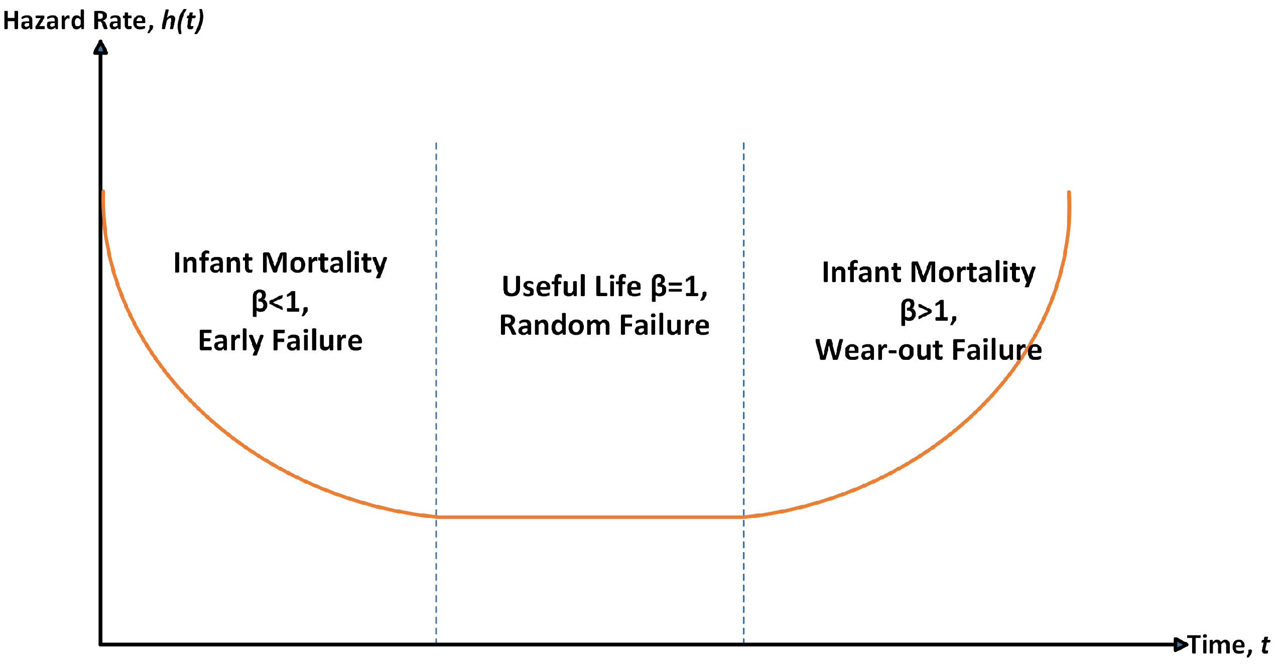
where the denominator $1-F\left(t\right)$ in Equation (3) represents the reliability function. The behavior of the hazard function for different values of $\beta$ can be represented by the well-known bathtub curve, which consists of three regions (Figure 1) [20,21]:

• Infant mortality phase ($\beta <1$): Characterized by a relatively high failure rate during the early life of the component.
• Useful life or burn-in phase ($\beta =1$): Characterized by a stable failure behavior with no clear time-dependent increase or decrease.
• Wear-out or end-of-life phase ($\beta >1$): Characterized by an increasing failure rate as the component ages and approaches the end of its lifespan.

Figure 1. The bathtub curve of the hazard function, where the orange line indicates the division of the three phases.

Figure 1. The bathtub curve of the hazard function, where the orange line indicates the division of the three phases.

As mentioned before, the CDF of the Weibull distribution plays an important role in this study. After fitting the Weibull model to the CCTV lifespan data, the CDF allows direct analysis of failure progression over time. Using the fitted CDF, this study estimates failure percentiles and corresponding time points. These estimates support practical predictions, such as identifying the operating time at which a specified proportion of CCTV components is expected to fail.

3.3. Mean Time to Failure (MTTF)

The MTTF refers to the expected time to failure for a non-repairable system, representing the average operating lifespan of a device [22]. It is widely used as a maintenance metric or reliability indicator, particularly for equipment that cannot or should not undergo repair. The MTTF can be calculated from the two-parameter Weibull distribution as:

$$MTTF=\eta \mathsf{\Gamma }\left(1+{\displaystyle \frac{1}{\beta }}\right),$$

(4)

where $\beta$ and $\eta$ denote the shape and scale parameters, respectively. The function $\mathsf{\Gamma }(·)$ denotes the Gamma function.

3.4. Reliability Function

For the Weibull distribution, $F\left(t\right)$ represents the probability that a component or system fails at or before a specified time t. In contrast, the reliability function, denoted as $R\left(t\right)$, is its complement and is often referred to as the survival function. It expresses the probability that the component continues to operate without failure beyond time t. Mathematically, this relationship is given by $R\left(t\right)=1-F\left(t\right)$. Substituting the Weibull CDF yields:

$$R\left(t\right)=e^{-{\left(\frac{t}{\eta }\right)}^{\beta }}$$

(5)

3.5. Method of Parameter Estimation in the Weibull Distribution

This study evaluates three analytical approaches for estimating the parameters of the Weibull distribution. The details of each estimator are outlined below:

3.5.1. The Maximum Likelihood Method (MLM)

The Maximum Likelihood Method (MLM) is employed to estimate the two parameters, $\eta$ (scale) and $\beta$ (shape) [23]. To optimize $\eta$ and $\beta$, we assume that $x_1,x_2,\dots ,x_n$ (or equivalently $t_1,t_2,\dots ,t_n$) are independent and identically distributed Weibull random variables, each following the PDF defined in Equation (1). With $\eta$ and $\beta$ treated as unknowns, the MLM is applied [24]. The likelihood function for $x_1,x_2,\dots ,x_n$ (or $t_1,t_2,\dots ,t_n$) can then be derived from Equation (1) as follows:

$$L\left(\eta ,\beta \right)=\prod _{i=1}^{n}f\left(x_i\right)={\eta }^n{\beta }^n{\left(\prod _{i=1}^n{x}_i\right)}^{\beta -1}exp\left(-\sum _{j=1}^n{\left({\displaystyle \frac{x_i}{\eta }}\right)}^{\beta }\right)$$

(6)

Taking the natural logarithm of Equation (6) yields the log-likelihood function:

$$\ln L(\eta ,\beta )=n\ln \eta -n\ln \beta +\left(\beta -1\right)\sum _{i=1}^n\ln x_i-\sum _{i=1}^n{\left({\displaystyle \frac{x_i}{\eta }}\right)}^{\beta }$$

(7)

By differentiating Equation (7) with respect to $\eta$ and $\beta$, we obtain:

$$\begin{array}{cc}\hfill {\displaystyle \frac{\partial }{\partial \eta }}\ln L(\eta ,\beta )& =-{\displaystyle \frac{n\beta }{\eta }}+\sum _{i=1}^n{({\displaystyle \frac{x_i}{\eta }})}^{\beta }({\displaystyle \frac{\beta }{\eta }})\hfill \end{array}$$

(8)

$$\begin{array}{cc}\hfill {\displaystyle \frac{\partial }{\partial \beta }}\ln L(\eta ,\beta )& ={\displaystyle \frac{n}{\beta }}-n\ln y+\sum _{i=1}^n\ln x_i-\sum _{i=1}^n{({\displaystyle \frac{x_i}{\eta }})}^{\beta }(\ln x-\ln y)\hfill \end{array}$$

(9)

Equating these to zero shows that the maximum likelihood estimates (MLEs) $(\widehat{\eta },\widehat{\beta })$ satisfy:

$$\begin{array}{cc}\hfill {\displaystyle \frac{n\beta }{\widehat{\eta }}}& =\sum _{i=1}^n\left({\displaystyle \frac{x_i}{\eta }}\right)\left({\displaystyle \frac{\beta }{\eta }}\right)\hfill \end{array}$$

(10)

$$\begin{array}{cc}\hfill {\displaystyle \frac{n}{\widehat{\beta }}}+\sum _{i=1}^n\ln x_i& =n\ln y+\sum _{i=1}^n{\left({\displaystyle \frac{x_i}{\eta }}\right)}^{\beta }(\ln x-\ln y)\hfill \end{array}$$

(11)

or equivalently,

$$\begin{array}{cc}\hfill \eta & ={\left({\displaystyle \frac{{\sum }_{i=1}^n{x}_i^{\beta }}{n}}\right)}^{{\displaystyle \frac{1}{\beta }}}\hfill \end{array}$$

(12)

$$\begin{array}{cc}\hfill \beta & ={\left({\displaystyle \frac{{\sum }_{i=1}^n{x}_i^{\beta }\ln \left(x_i\right)}{{\sum }_{i=1}^n{x}_i^{\beta }}}-{\displaystyle \frac{{\sum }_{i=1}^n\ln \left(x_i\right)}{n}}\right)}^{-1}\hfill \end{array}$$

(13)

Equations (6)–(13) are typically solved using numerical methods to obtain the estimated $\widehat{\beta }$ first, and then $\widehat{\beta }$ is substituted into Equation (12) to obtain $\eta$. For further details on the maximum likelihood method, readers may refer to [1]. Rather than elaborating further on this method, this alternative method is computationally simpler and, according to simulation studies, often provides more accurate estimates of $(\eta ,\beta )$, particularly when the sample size n is relatively small.

3.5.2. Method of Moments (MOM)

The Method of Moments (MOM) is commonly utilized to estimate the parameters of the Weibull distribution. Let the observed lifespans be denoted by $x_1,x_2,\dots ,x_n$ (or equivalently $t_1,t_2,\dots ,t_n$). An unbiased estimator for the $k^{\mathrm{th}}$ moment can then be defined as:

$${\widehat{m}}_k={\displaystyle \frac{1}{n}}\sum _{t=1}^n{x}_t^k,$$

(14)

where ${\widehat{m}}_k$ represents the sample estimate of the $k^{\mathrm{th}}$ moment. For the Weibull distribution defined in Equation (1), the corresponding theoretical $k^{\mathrm{th}}$ moment is expressed as:

$${\mu }_k={(1/{\eta }^k)}^{{\displaystyle \frac{k}{\beta }}}\mathsf{\Gamma }\left(1+{\displaystyle \frac{k}{\beta }}\right),$$

(15)

where $\mathsf{\Gamma }(·)$ is the Gamma function as defined in Equation (4); the first and second moments about zero can be obtained as follows:

$${\widehat{m}}_1={\widehat{\mu }}_1={(1/\eta )}^{{\displaystyle \frac{1}{\beta }}}\mathsf{\Gamma }\left(1+{\displaystyle \frac{1}{\beta }}\right),$$

(16)

and

$${\widehat{m}}_2={\left({\displaystyle \frac{1}{\eta }}\right)}^{{\displaystyle \frac{2}{\beta }}}\left[\mathsf{\Gamma }\left(1+{\displaystyle \frac{2}{\beta }}\right)-\mathsf{\Gamma }{\left(1+{\displaystyle \frac{1}{\beta }}\right)}^2\right]$$

(17)

By dividing the square of ${\widehat{m}}_1$ by ${\widehat{m}}_2$, we obtain an expression that depends only on $\beta$:

$${\displaystyle \frac{{\widehat{\mu }}^2}{{\widehat{\sigma }}^2+{\widehat{\mu }}^2}}={\displaystyle \frac{{\mathsf{\Gamma }}^2\left(1+\frac{1}{\beta }\right)}{\mathsf{\Gamma }\left(1+\frac{2}{\beta }\right)}}.$$

(18)

where

$$\begin{array}{cc}\hfill \widehat{\mu }& =E\left(x_t\right)={\displaystyle \frac{1}{n}}\sum _{t=1}^n{x}_t,\hfill \end{array}$$

(19a)

$$\begin{array}{cc}\hfill {\widehat{\sigma }}^2& =E\left(x_t^2\right)-{\left[E\left(x_t\right)\right]}^2,\hfill \end{array}$$

(19b)

$$\begin{array}{cc}\hfill Z& ={\displaystyle \frac{1}{\beta }}.\hfill \end{array}$$

(19c)

After determining $\beta$ numerically from Equation (18), the scale parameter ${\eta }_{\mathrm{MOM}}$ can be estimated using the following relation:

$${\widehat{\eta }}_{\mathrm{MOM}}={\displaystyle \frac{\widehat{\mu }}{\mathsf{\Gamma }\left(1+\frac{1}{\widehat{\beta }}\right)}}.$$

(20)

3.5.3. Least Squares Method (LSM)

This study applies the Least Squares Method (LSM) to estimate Weibull parameters using a linearized representation of the model. The method fits a straight line to transformed data in order to obtain parameter estimates.

Consider a dataset consisting of n paired observations $(x_t,y_t)$, where $t=1,2,\dots ,n$. The Least Squares Method fits a linear relationship to the observed data. The linear model is given by $y_t=a+b{x}_t$.

Accordingly, the sum of squared errors (SSE) to be minimized is defined as:

$$Q(x;\alpha ,\beta )=\sum _{t=1}^n{(y_t-\alpha -\beta x_t)}^2.$$

(21)

To obtain the estimators of $\alpha$ and $\beta$, we differentiate $Q(x;\alpha ,\beta )$ with respect to both parameters and set the resulting expressions equal to zero. This yields the following system of equations:

$${\displaystyle \frac{\partial Q}{\partial \alpha }}=-2\sum _{t=1}^n(y_t-\alpha -\beta x_t)=0,$$

(22)

$${\displaystyle \frac{\partial Q}{\partial \beta }}=-2\sum _{t=1}^n{x}_t(y_t-\alpha -\beta x_t)=0.$$

(23)

Expanding and solving Equations (22) and (23) simultaneously, we obtain the following least squares estimators:

$$\widehat{\beta }={\displaystyle \frac{n\sum x_t{y}_t-\sum x_t\sum y_t}{n\sum x_t^2-{\left(\sum x_t\right)}^2}},$$

(24)

and

$$\widehat{\alpha }=\overline{y}-\widehat{\beta }\overline{x},$$

(25)

where $\overline{x}={\displaystyle \frac{1}{n}}{\sum }_{t=1}^n{x}_t$ and $\overline{y}={\displaystyle \frac{1}{n}}{\sum }_{t=1}^n{y}_t$ represent the sample means of x and y, respectively. In the context of the Weibull model, the intercept term can be expressed as:

$$\widehat{\eta }=\exp \left(-{\displaystyle \frac{\widehat{\alpha }}{\widehat{\beta }}}\right),$$

(26)

where $\widehat{\alpha }$ and $\widehat{\beta }$ are the unbiased estimators of $\alpha$ and $\beta$, respectively.

3.5.4. Mean Square Error (MSE) for Accuracy of Weibull Distribution Parameters

This study uses the MSE to evaluate and compare the accuracy of the Weibull parameter estimation methods. The MSE is defined as:

$$\mathrm{MSE}={\displaystyle \frac{1}{n}}\sum _{i=1}^n{\left[\widehat{F}\left(x_i\right)-F\left(x_i\right)\right]}^2.$$

(27)

Here, $\widehat{F}\left(x_i\right)$ (or equivalently $\widehat{F}\left(t_i\right)$) is obtained by substituting the estimated parameters $\widehat{\eta }$ and $\widehat{\beta }$, derived from each estimation method, into the theoretical distribution function. In contrast, $F\left(x_i\right)$ represents the empirical distribution function defined in Equation (1).

3.6. Kolmogorov–Smirnov Test (K–S Test)

The Kolmogorov–Smirnov one-sample test (K–S test) is commonly used to evaluate whether a given random sample follows a specified continuous probability distribution.

We set the null hypothesis (H₁) that the observed data come from the assumed distribution against the alternative hypothesis (H₂) that they do not; the hypotheses for this study are formulated as follows:

H₁. 

The data follow the Weibull distribution.

H₂. 

The data do not follow the Weibull distribution.

The Kolmogorov–Smirnov test is defined as:

$$D_n=\underset{x}{\max }\left|F_n\left(x\right)-F\left(x\right)\right|,$$

(28)

In this equation, $F_n\left(x\right)$ denotes the empirical distribution function, and $F\left(x\right)$ denotes the Weibull CDF under the null hypothesis. This study compares the test statistic $D_n$ with the critical value $D_{(n,\alpha )}$ at a significance level of $\alpha =0.05$. The null hypothesis is supported when $D_n$ remains below the critical threshold. Equivalently, the test can be interpreted using the associated p-value, where the null hypothesis is supported when the p-value exceeds $\alpha$. Both criteria indicate no statistically significant deviation from the Weibull distribution.

3.7. Anderson–Darling Test (AD Test)

The Anderson–Darling (AD) test can be used to analyze whether sample data fit a specified theoretical distribution. The AD test places greater emphasis on deviations in the tails of the distribution [25]. This property makes the AD test suitable for reliability analysis, where tail behavior directly relates to extreme failures.

The AD test in this study has the same hypothesis structure as the K–S test. The null hypothesis of the AD test assumes that the observed data follow the Weibull distribution. Conversely, the alternative hypothesis assumes otherwise. The hypotheses are defined as follows:

H₃. 

The data follow a Weibull distribution.

H₄. 

The data do not follow a Weibull distribution.

3.8. Bootstrapping Analysis

Bootstrapping is a powerful non-parametric resampling technique. This technique is used to estimate the sampling distribution when the sample size is small or the theoretical distribution is unknown.

In this study, we utilize bootstrapping to assess the uncertainty of the mean failure time estimated from the Weibull distribution because the sample size of our dataset is small. By using resampling, we construct confidence intervals for the mean failure time and to examine the stability of the estimate across different sample sizes. This approach provides a data-driven measure of variability without introducing additional distributional assumptions and complements the parametric Weibull model [26,27].

4. Implementation

In this study, we estimate lifespan, with a case study of indoor CCTV units installed in two areas. The analysis follows four main steps.

• We evaluated the datasets from both areas using GOF tests to assess whether our dataset fitted the Weibull distribution. We utilized the K–S and AD tests, and Q–Q plots. Those were used for visual verification of fit to the Weibull distribution.
• We applied three analytical methods to estimate the Weibull parameters, specifically, the shape and scale.
• We compared and measured the accuracy of each parameter estimation method.
• We validated the Weibull analysis results through a bootstrapping approach to confirm the robustness of the fitted distribution.

After completing these four analytical steps, we evaluated the CCTV lifespan and reliability under real operating conditions in Areas A1 and A2. The dataset and source code used in this study are publicly available in a GitHub repository (https://github.com/vanvisach/CCTVP/ (accessed on 1 February 2026)).

4.1. The Comprehensive Lifespan Data

Lifespan refers to the duration of a CCTV system’s operational life. When time serves as the measure of life, the observations are referred to as time-to-failure (TTF) data. Lifespan data can take different forms and offer distinct insights into the reliability and durability of electronic systems. Therefore, the analytical approach should align with the characteristics of the available data.

In this study, we focus on complete data, which provide the exact TTF values for each device (for example, CCTV systems that usually fail after about 10 years of operation). To demonstrate the proposed analysis, we consider a case study involving CCTV systems installed in 2010. While some units remain operational, others have failed over time. Our goal is to analyze their reliability characteristics and identify the estimated lifespan range to support maintenance planning and replacement decisions.

4.2. Data Collection

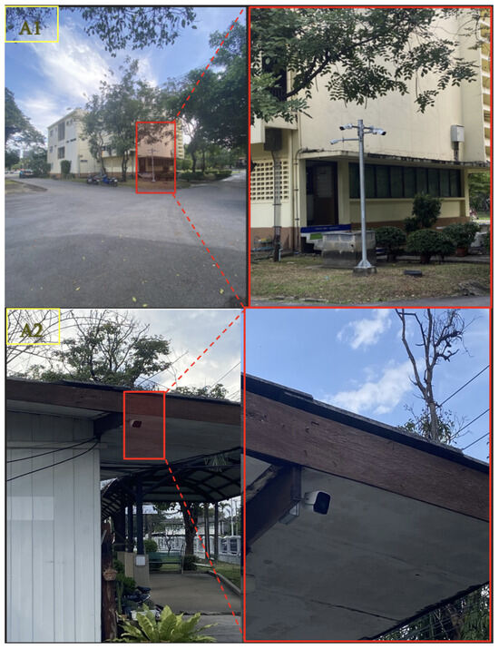
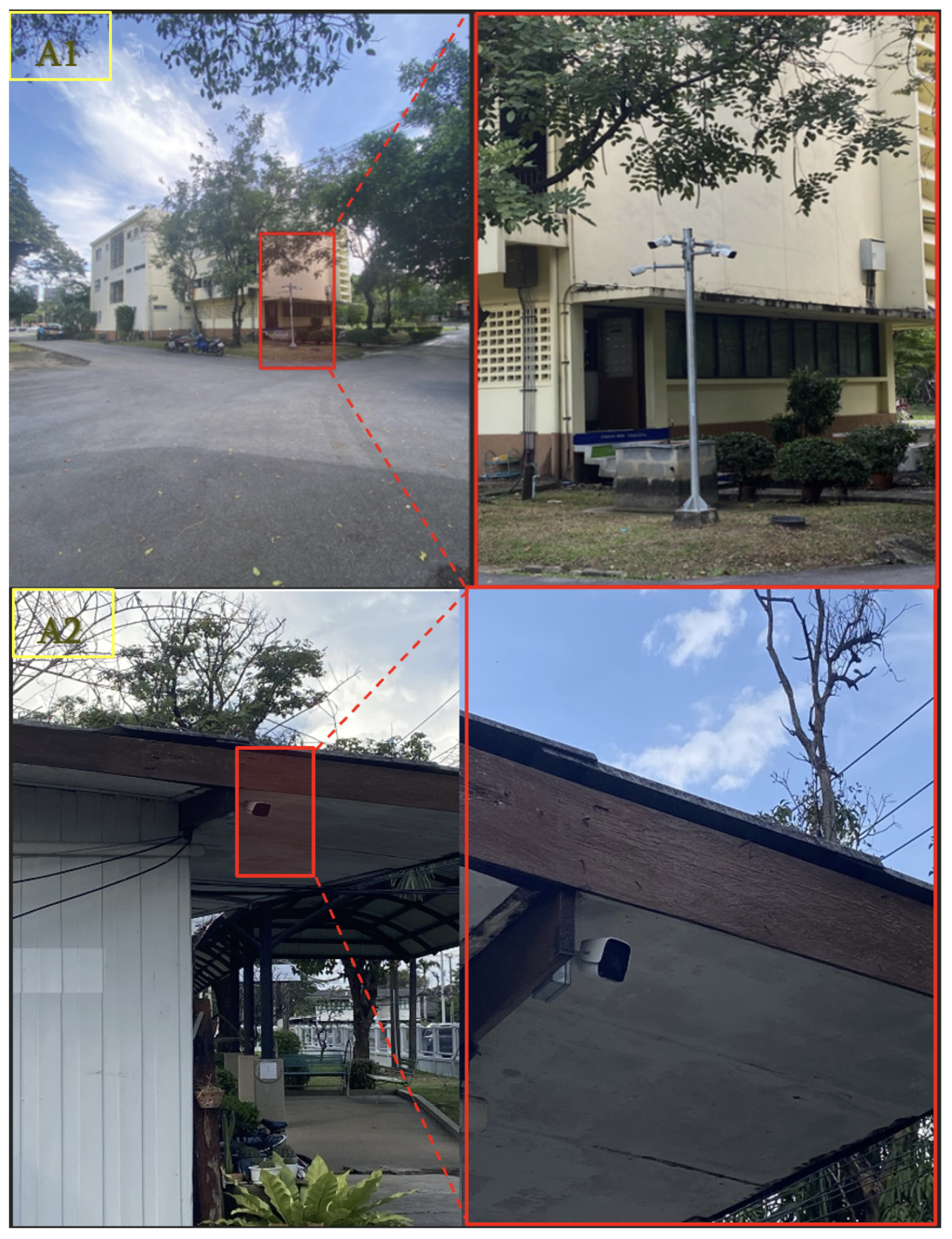
Our dataset of this case study collected CCTV systems installed between 2010 and 2020 in two distinct areas, denoted as A1 and A2. These areas differ in geographical characteristics and climatic conditions within Thailand. Area A1 is located in the central region, where the average temperature is approximately 30 °C, with intermittent rainfall. Area A2 is located in the southern region, which experiences a hotter climate, with an average temperature of approximately 35 °C and frequent rainfall throughout the year. Figure 2 shows where the systems are installed outdoors across various service locations.

Figure 2. CCTV installations in two service areas: the (top) image represents Area A1, and the (bottom) image represents Area A2.

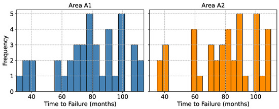
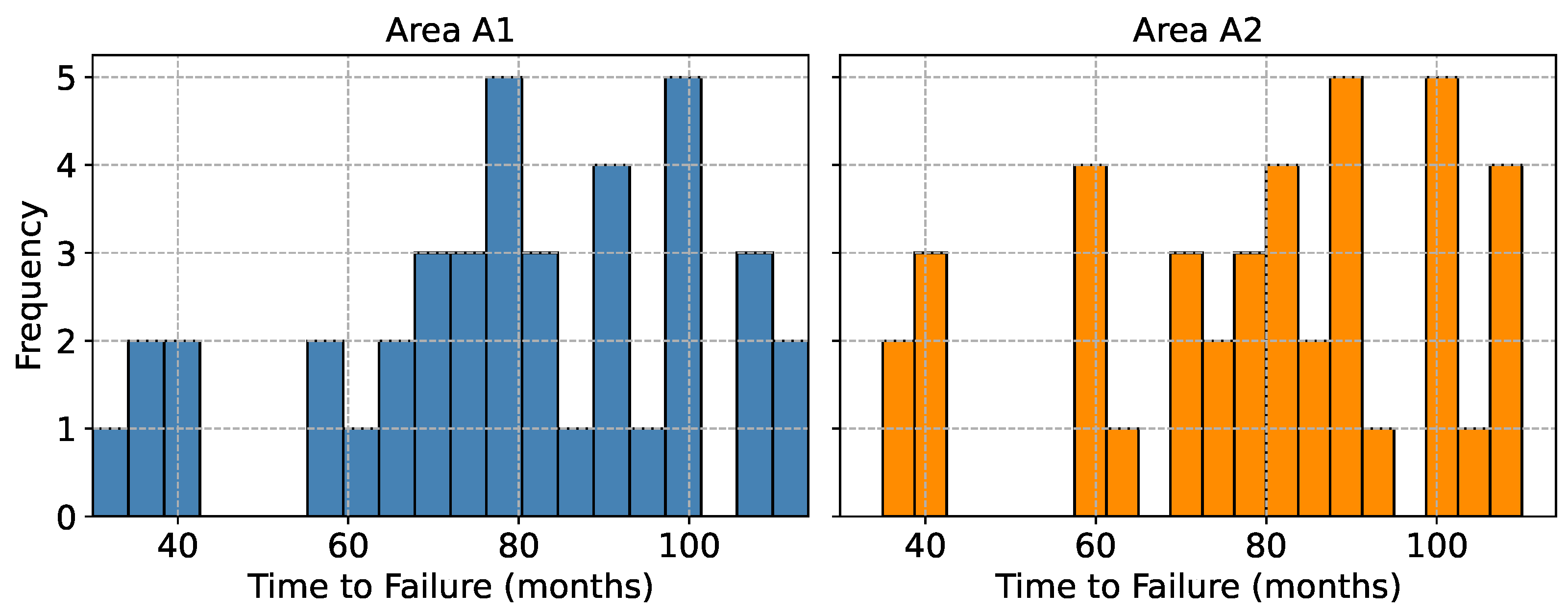
Note that each area includes approximately 40 CCTV samples. All units share the same make and model, and the distribution of their TTF values is shown in Figure 3.

Figure 3. Histogram of TTF for Areas A1 and A2.

4.3. The Goodness of Fit Test (GOF)

The GOF of the Weibull model was evaluated using the K–S test and the A–D test. Since the Weibull parameters were estimated from the observed data, p-values for both tests were obtained using a parametric bootstrap (Monte Carlo) [25] procedure to account for parameter estimation uncertainty.

For the K–S test, the empirical CDF was compared with the fitted Weibull CDF, and the observed K–S statistic $D_s$ was computed for each area. Bootstrap p-values were estimated at a significance level of $\alpha =0.05$. As shown in Table 1, the bootstrap p-values for both Areas A1 and A2 exceed the selected significance level, indicating no evidence for rejecting the Weibull assumption.

Table 1. KS goodness-of-fit test results for the Weibull model in Areas A1 and A2.

No.	Area Name	K–S Statistic, ${\mathit{D}}_{\mathit{s}}$	p-Value (Bootstrap)	Decision
1	A1	0.0925	0.5057	Fail to reject Weibull
2	A2	0.0888	0.5742	Fail to reject Weibull

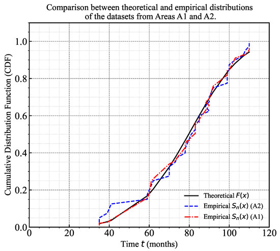
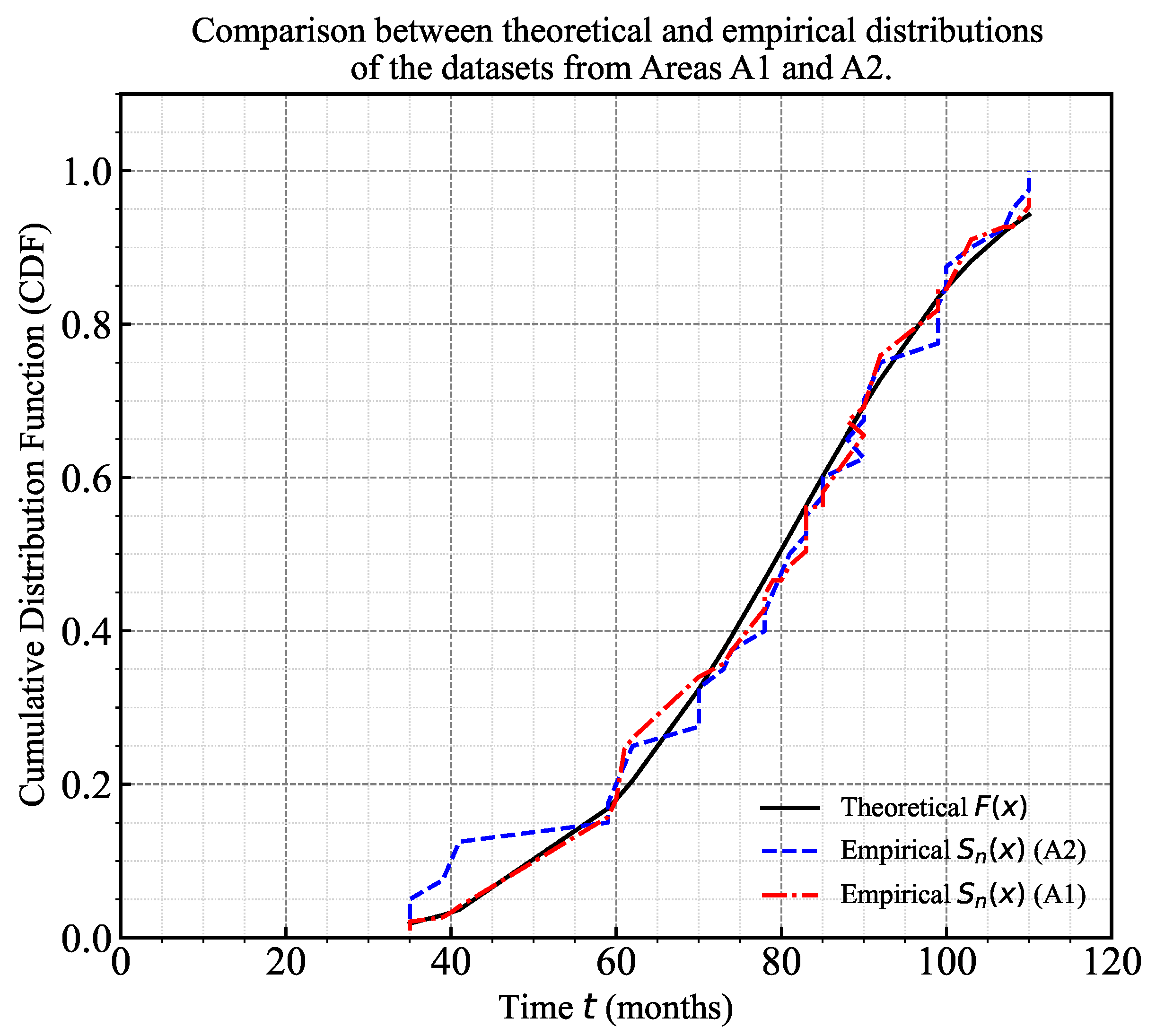
Figure 4 illustrates the agreement between the empirical and theoretical distributions, while Table 1 summarizes the K–S test statistics and corresponding bootstrap p-values for Areas A1 and A2.

Figure 4. Comparison between the theoretical and empirical distributions of the datasets from Areas A1 and A2.

Following the K–S test, the goodness of fit was further assessed using the Anderson–Darling (AD) test, which places greater emphasis on the tail behavior of the distribution and therefore complements the K–S test. The bootstrap p-values for the AD test were computed using the same parametric bootstrap procedure.

As shown in Table 2, the bootstrap p-values for both Areas A1 and A2 are greater than the significance level of $\alpha =0.05$. Therefore, the null hypothesis that the data follow a Weibull distribution cannot be rejected. These results are consistent with the findings of the bootstrap-based K–S test.

Table 2. AD goodness-of-fit test results for the Weibull distribution in Areas A1 and A2.

No.	Area Name	AD Statistic, ${\mathit{A}}^2$	p-Value (Bootstrap)	Decision
1	A1	0.5543	0.1534	Fail to reject Weibull
2	A2	0.4094	0.3558	Fail to reject Weibull

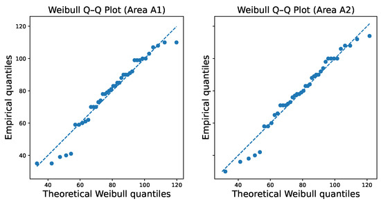
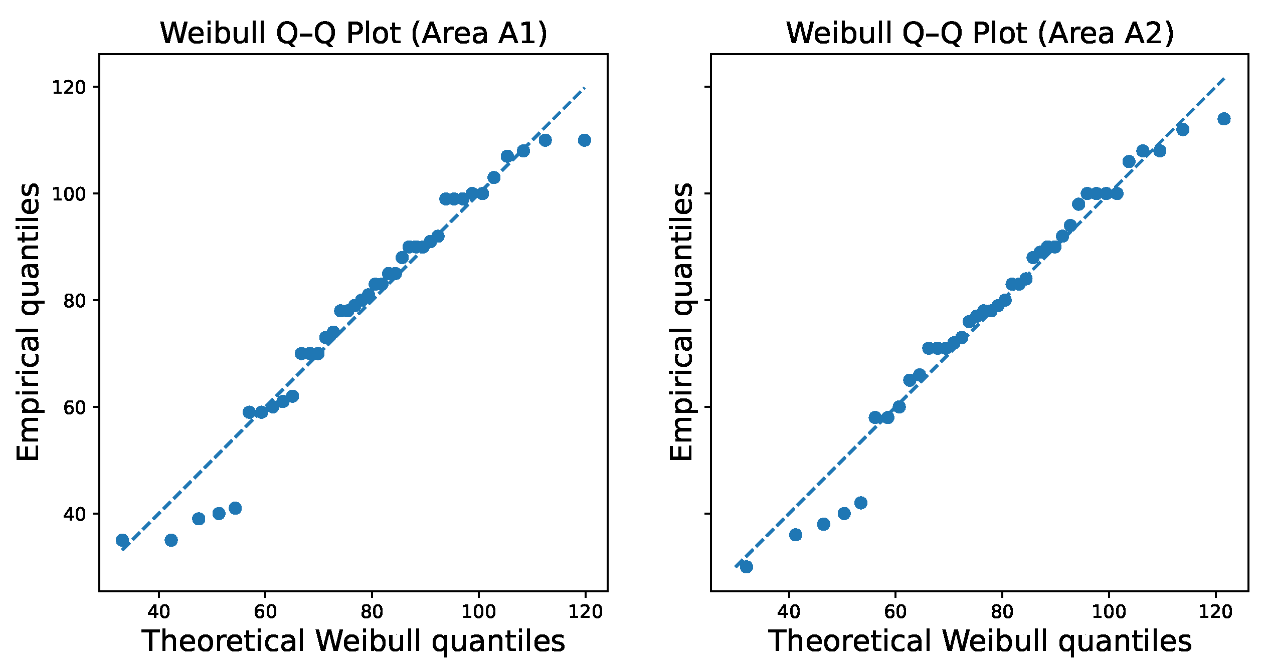
To further support these results, Q–Q plots were used for visual assessment. Figure 5 shows the Q–Q plots comparing empirical failure-time quantiles with theoretical quantiles from the fitted Weibull models.

Figure 5. Weibull Q–Q plots comparing empirical failure-time quantiles with theoretical quantiles from the fitted Weibull models for Areas A1 and A2.

As shown in Figure 5, the Q–Q plots for both areas exhibit similar linear patterns. This analysis suggests that the Weibull model provides an appropriate fit for the two datasets and indicates consistency with the assumed distribution.

4.4. Estimating Parameters of Weibull Distributions

The shape ($\beta$) and scale ($\eta$) parameters are key parameters of the Weibull distribution, and numerous methods exist for estimating their values. In this study, three parameter estimation methods were employed.

We applied a parametric bootstrap approach to quantify uncertainty in the estimated Weibull parameters. In our study, the number of bootstrap replications is set to 2000. In each replication, a synthetic sample is generated from the fitted Weibull distribution. The model is then refit with the location parameter fixed at zero. The resulting bootstrap distributions are used to construct 95% confidence intervals for the parameters and derived reliability measures using the percentile method, and the results are shown in Table 3.

Table 3. Comparison of parameter estimation methods for Areas A1 and A2. Note that values in parentheses indicate 95% confidence intervals.

Area A1
Method	β	η	MSE
MOM	4.0646 (3.6952, 6.0858)	87.0231 (79.9421, 92.61881)	0.0011 (0.0004, 0.0035)
MLE	4.3881 (3.7241, 6.0569)	86.8207 (79.9618, 92.6850)	0.0010 (0.0004, 0.0035)
LSM	3.6347 (3.0846, 5.8855)	87.8119 (80.4643, 93.5676)	0.0017 (0.0004, 0.0056)
Area A2
Method	$\beta$	$\eta$	MSE
MOM	4.2018 (3.5591, 5.8437)	86.8026 (79.8533, 93.0541)	0.00152 (0.0005, 0.0035)
MLE	4.4000 (3.5855, 5.8315)	86.6425 (79.8781, 93.1180)	0.00150 (0.0005, 0.0035)
LSM	3.7239 (2.9698, 5.6665)	87.7368 (80.3996, 94.0392)	0.00192 (0.0005, 0.0056)

Like the results in Table 1, the MSE results indicate that the MLM yields the minimum values of 0.0010 and 0.0015; the corresponding parameters of A1 are $\beta =4.3881$ and $\eta =86.8207$ and those of A2 are $\beta =4.4000$ and $\eta =86.6425$. This suggests that the MLE stands out as the optimal method among the three estimation techniques. Subsequently, these optimal parameters were incorporated into our modeling process.

After selecting the optimal shape and scale parameters using the MLE approach, we applied the Weibull model to evaluate the lifespan of the CCTV systems. Because both study areas share similar environmental and operational conditions, this comparison provides consistent insights into reliability behavior. Our analysis examines failure behavior, survival characteristics, and expected lifetime to assess CCTV performance and durability.

4.5. The Simulation

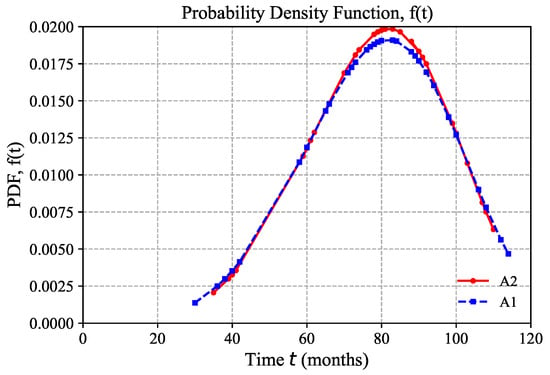
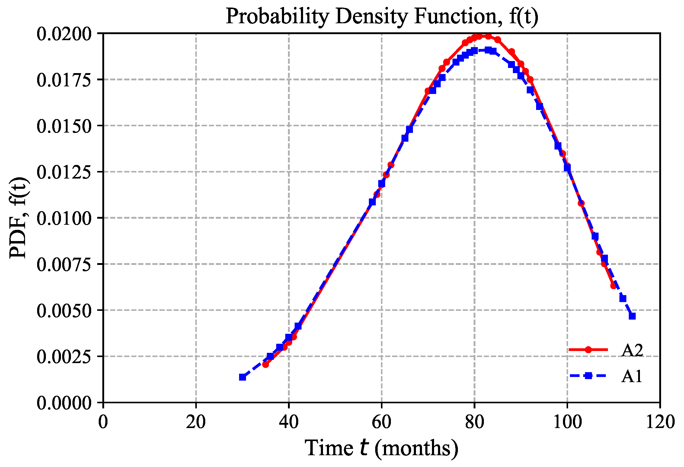
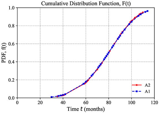
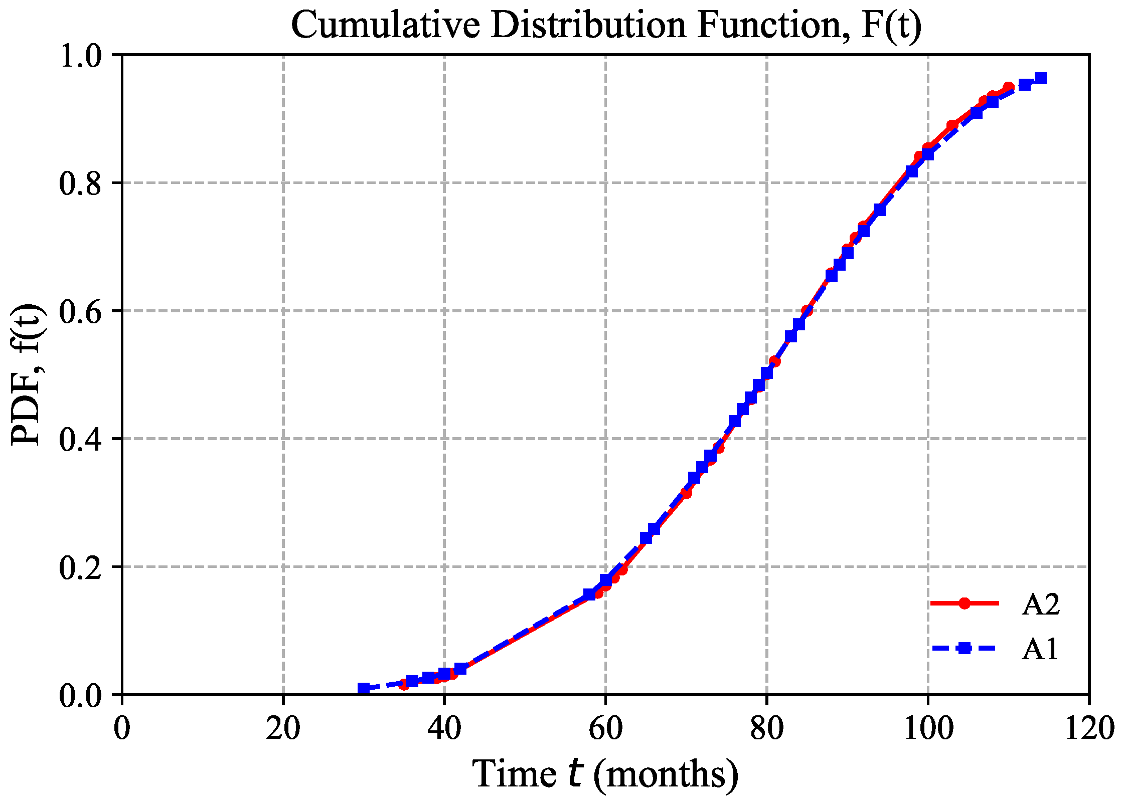
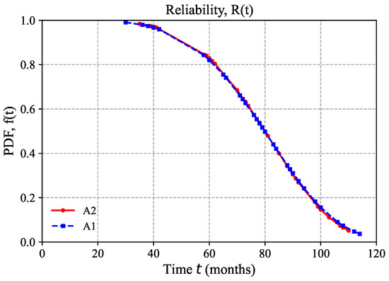
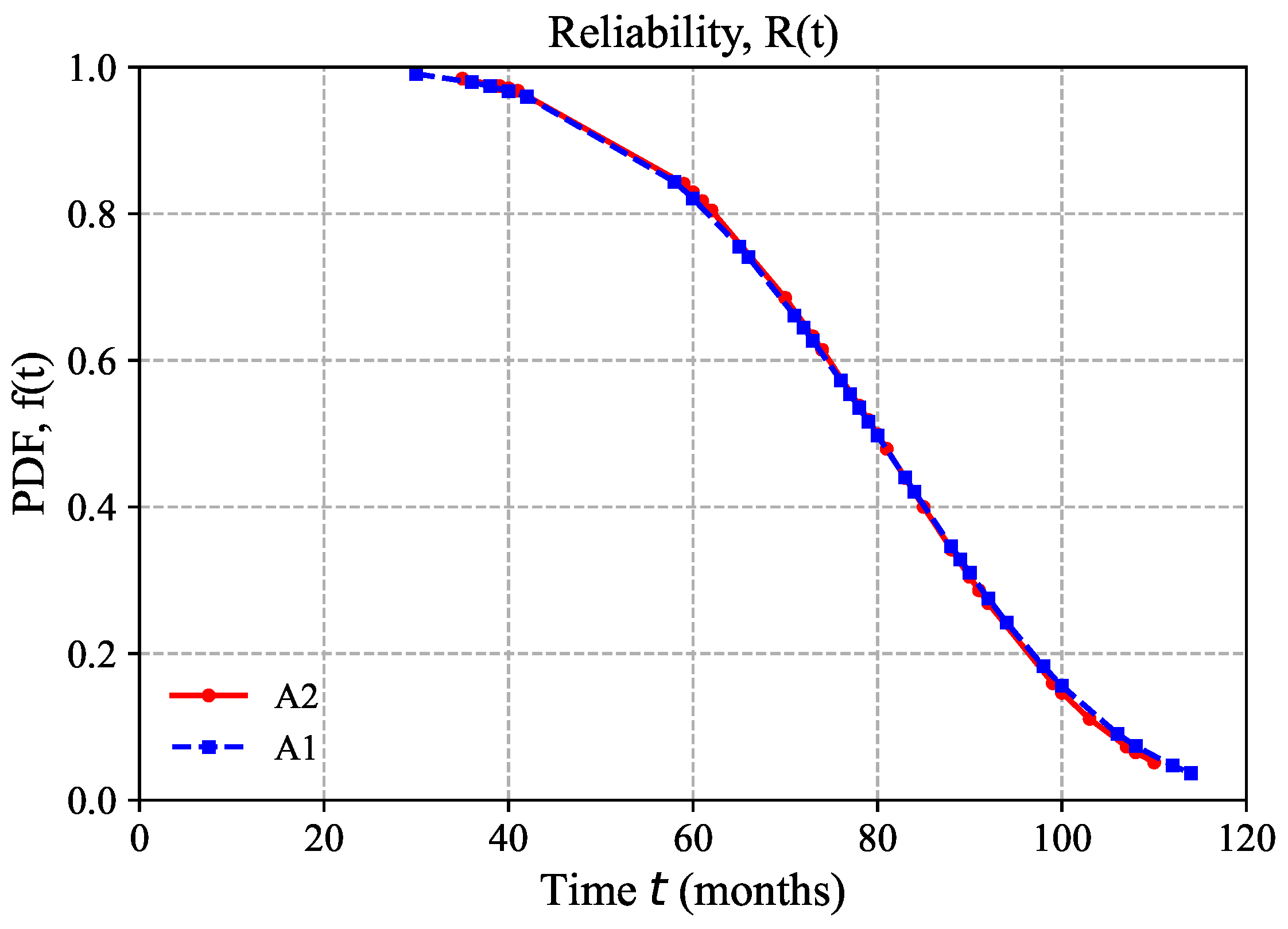
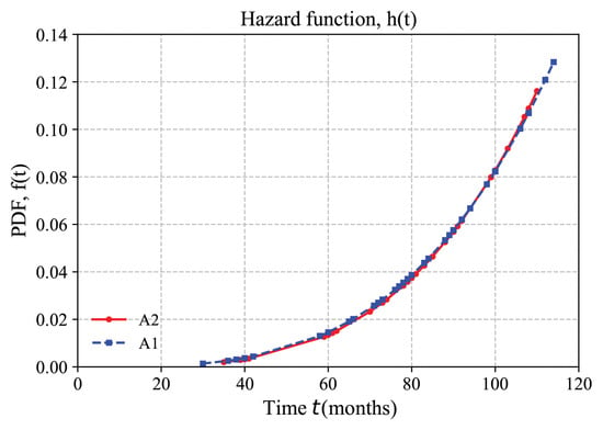
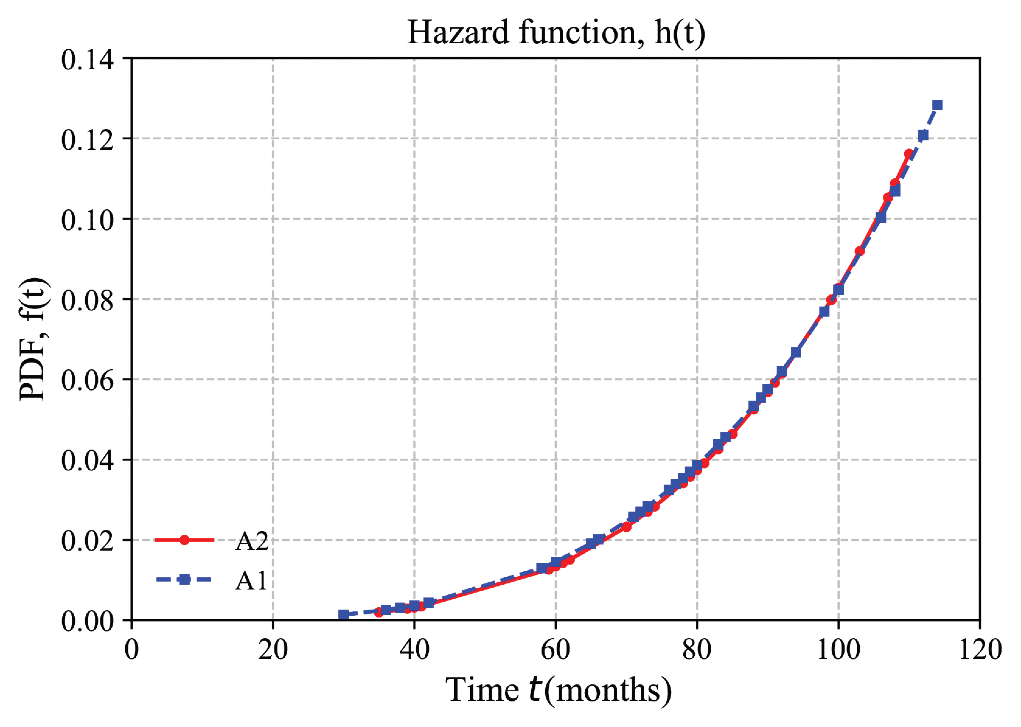
We performed a numerical simulation to determine the optimal Weibull parameters for the CCTV failure dataset collected from 2010 to 2020. The simulation evaluates three parameter estimation methods and compares their performance. For each method, we estimated the Weibull shape ($\beta$) and scale ($\eta$) parameters and computed the PDF, CDF, reliability function, and hazard function. We selected the most accurate estimation method based on the minimum MSE across these four functions. Figure 6, Figure 7, Figure 8 and Figure 9 illustrate the performance of the estimation methods for Areas A1 and A2.

Figure 6. Comparison of the PDF graphs for Areas A1 and A2.

Figure 7. Comparison of the CDF graphs for Areas A1 and A2.

Figure 8. Comparison of the reliability function graphs for Areas A1 and A2.

Figure 9. Comparison of the hazard function graphs for Areas A1 and A2.

Figure 6, Figure 7, Figure 8 and Figure 9 show that Areas A1 and A2 exhibit highly similar failure time characteristics. In Figure 6, both PDFs follow a bell-shaped pattern, indicating consistent lifetime behavior across the two areas. Figure 7 shows that the CDFs rise along almost identical trajectories, suggesting comparable cumulative failure probabilities. As shown in Figure 8, the reliability functions decrease at nearly the same rate, indicating similar survival tendencies for the CCTV devices. The hazard functions in Figure 9 increase steadily over time, showing an aging or wear-out failure pattern typical of electronic components. Among the three estimation methods, the MLE approach generates curves that align most closely with the empirical data. Table 1 summarizes the MSE-based comparison of all methods.

4.6. Bootstrapping Analysis for the Mean of the Weibull Distribution

In this subsection, we verified the estimated mean failure time derived from the Weibull distribution using a bootstrapping analysis. The bootstrapping analysis involved resampling the observed data (i.e., the recorded lifespans of the CCTV units) with replacement to generate multiple resampled datasets. If the Weibull model provides an appropriate description of the data, the mean failure times obtained from the bootstrap samples should be close to the theoretical mean of 6.6 years.

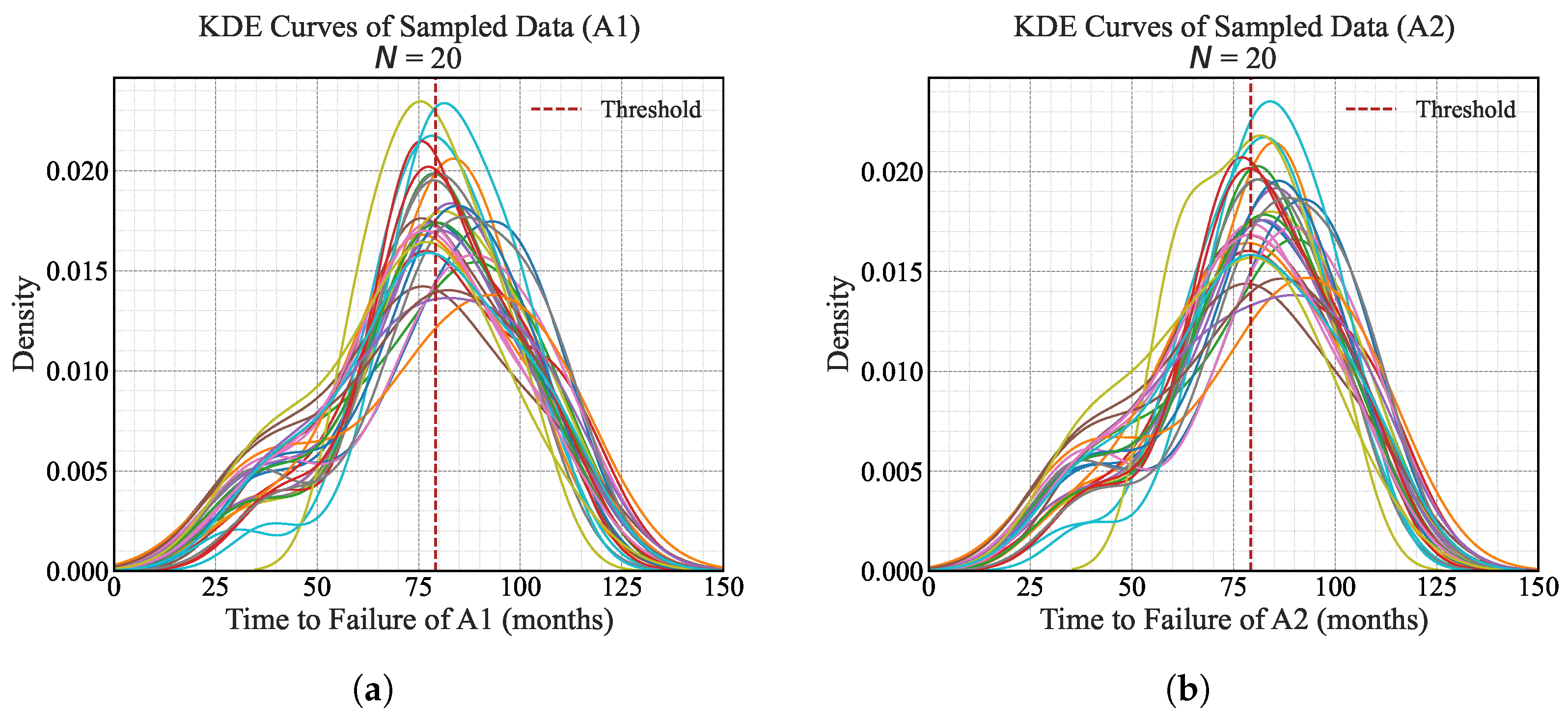
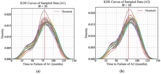
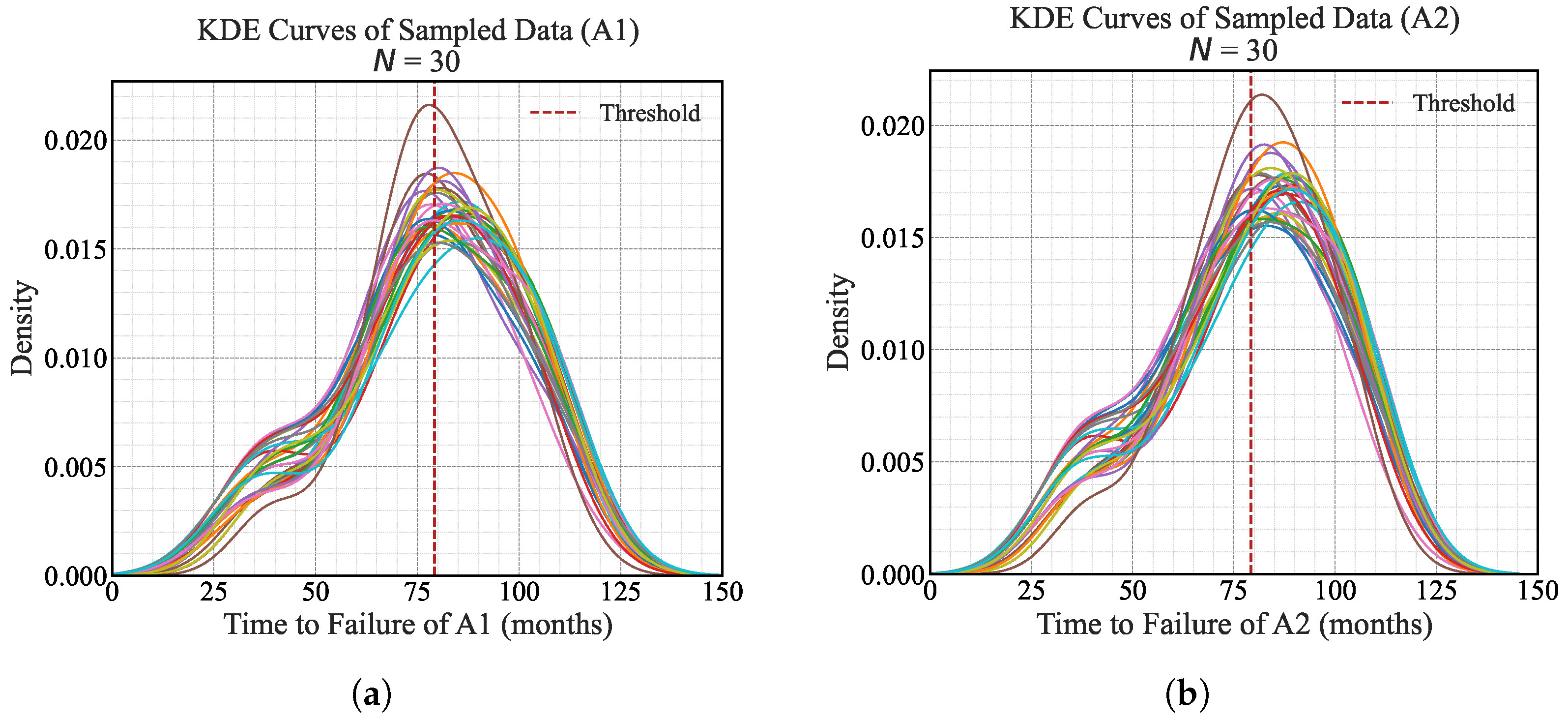
In our analysis, we resampled the data 30 times using three sample-size groups of 15, 20, and 30. These sizes represent small, medium, and relatively large subsets of the available data and reflect practical scenarios in which only limited failure records are available. In total, we generated 90 bootstrap samples for each camera area.

To quantify uncertainty, we used bootstrap confidence intervals (Bootstrap-CI) to compare the estimated mean failure time across different sample sizes. This approach allowed us to examine the stability and variability of the estimates under resampling [28]. Notably, we adopted a significance level of $\alpha =0.05$ for all the statistical tests in this study.

Table 4 reports the bootstrap confidence intervals of the mean failure time for different sample sizes in Areas A1 and A2. The confidence intervals across different sample sizes and areas show substantial overlap and include the theoretical mean failure time of 6.6 years (79 months). Thus, these results suggest that the estimated mean remains consistent across different data proportions and highlight the robustness of the Weibull-based lifespan evaluation.

Table 4. Bootstrap-CI for the mean failure time (months) for different sample sizes in Areas A1 and A2.

Sample Size	Area A1	Area A2
15	(66.7002, 85.0207)	(70.7164, 82.9005)
20	(70.7410, 82.9255)	(67.0791, 85.3895)
30	(68.0224, 84.7273)	(70.3658, 80.6322)

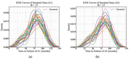
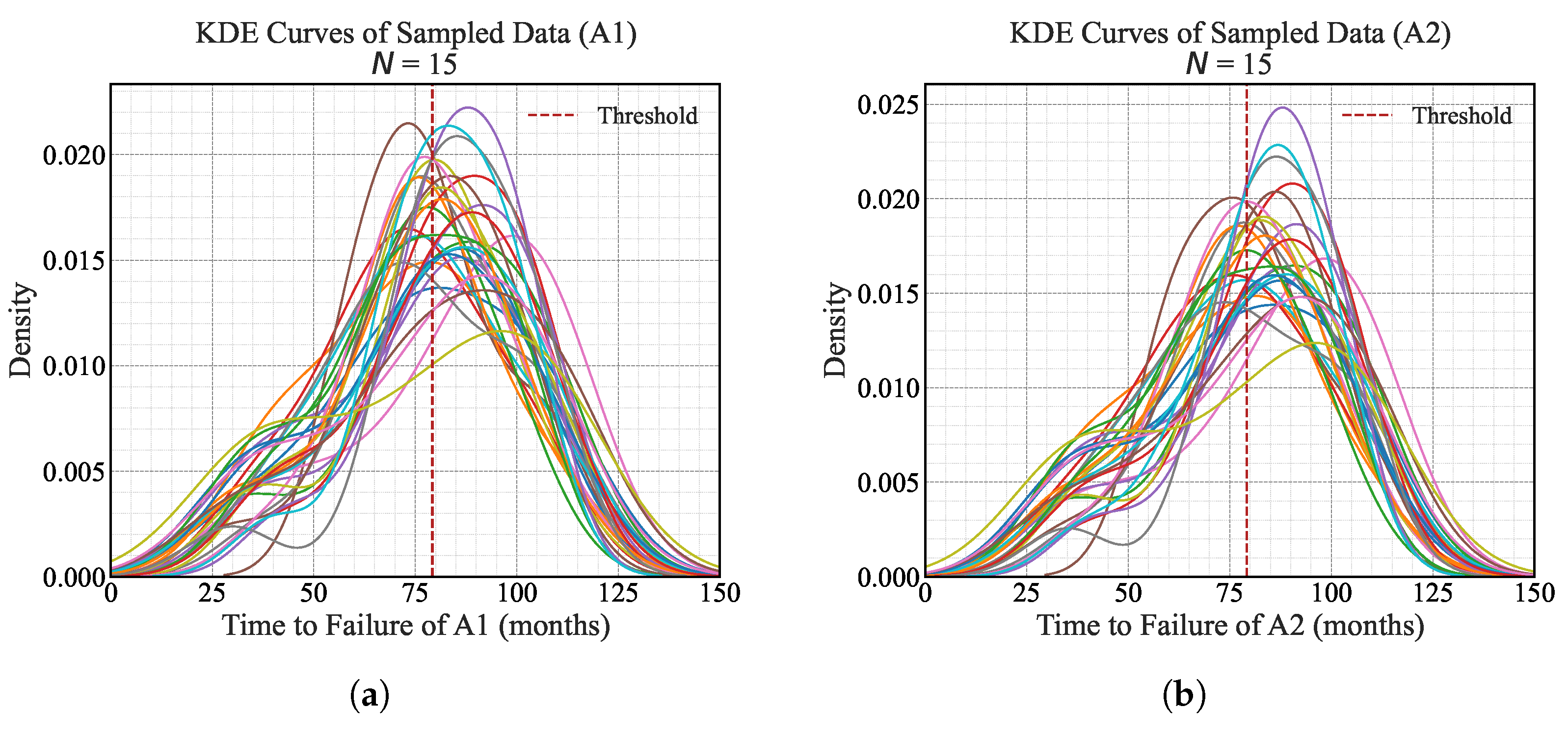
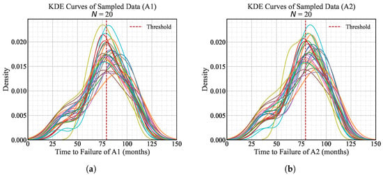
To complement this analysis, Figure 10, Figure 11 and Figure 12 present the distributions for each sample-size group. The vertical dashed line denotes the theoretical mean failure time of 6.6 years.

Figure 10. Bootstrapped mean failure time distribution (15 samples). Colored lines represent individual bootstrap sample realizations.

Figure 11. Bootstrapped mean failure time distribution (20 samples). Colored lines represent individual bootstrap sample realizations.

Figure 12. Bootstrapped mean failure time distribution (30 samples). Colored lines represent individual bootstrap sample realizations.

By visualizing all histograms of the resampled datasets, we observed that the mean failure times were close to 6.6 years. Upon reducing the number of samples or changing the CCTV area, the mean failure time remains approximately equal to 6.6 years. However, visual inspection may be subject to bias. Therefore, we conducted hypothesis testing for each resample by defining the null hypothesis (H₁) that the mean failure time of each sample is equal to 6.6 years, with a significance level ($\alpha$) of 0.05.

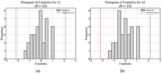
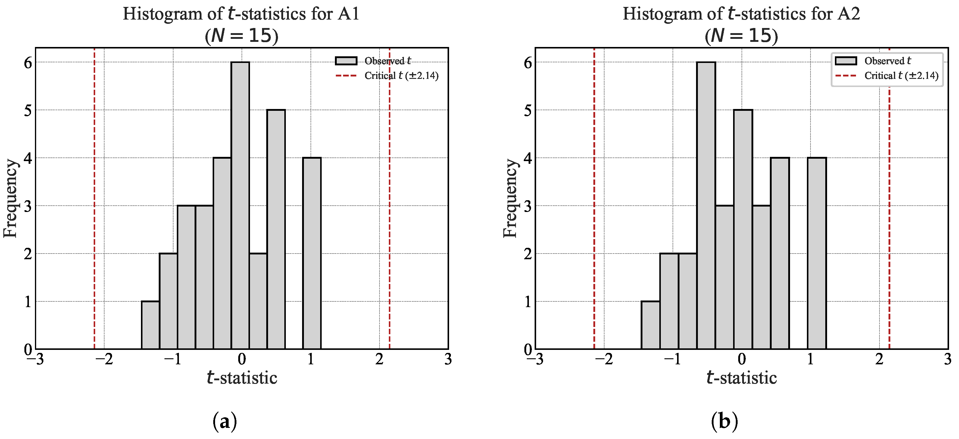
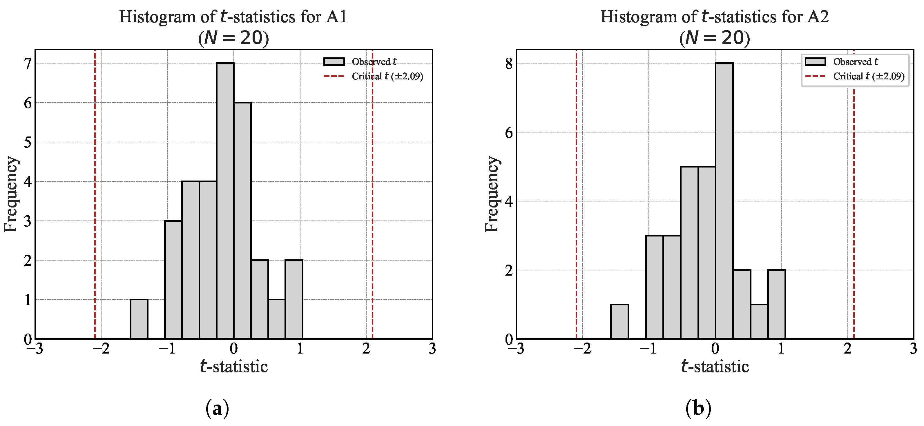
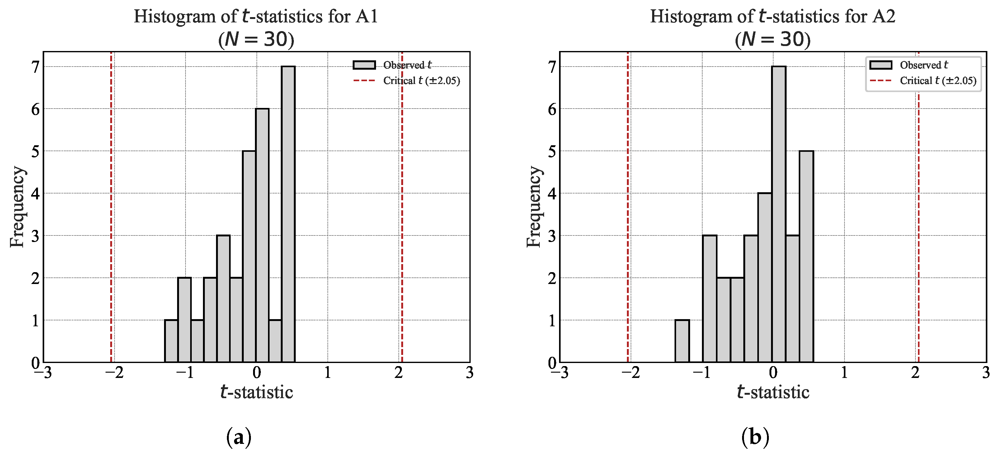
For each resampled dataset, a two-tailed t-test was performed to evaluate whether the sample mean differed significantly from the theoretical mean of 6.6 years. The resulting t-statistics were then summarized and visualized as histograms for each sample-size group. All histograms are shown as in Figure 13, Figure 14 and Figure 15.

Figure 13. Distribution of t-statistics from two-tailed t-tests based on 15-sample resampling.

Figure 14. Distribution of t-statistics from two-tailed t-tests based on 20-sample resampling.

Figure 15. Distribution of t-statistics from two-tailed t-tests based on 30-sample resampling.

All the t-values for the 15-, 20-, and 30-sample resampling groups fell within the critical region corresponding to a significance level of 0.05. These results indicate that all resampled means were statistically consistent with the theoretical Weibull mean of 6.6 years. This provides strong evidence that the Weibull model adequately represents the data in terms of the mean failure time.

Overall, the mean failure times obtained from the resampled datasets are statistically consistent with the theoretical mean of 6.6 years derived from the Weibull distribution. This finding supports the idea that the Weibull model provides a reasonable representation of the data in terms of the mean failure time. Therefore, the Weibull model can be considered an appropriate description of our data in terms of the mean.

4.7. Analysis and Discussion

The results show that the MLE provides consistent Weibull parameters for both study areas. The estimated MTTF is approximately 6.6 years, which represents the average operational lifespan of the CCTV systems. This value exceeds the typical reference lifespan of electronic products, which is often reported to be around 5 years based on MTBF considerations in Thai industrial standards. The extended operational lifespan supports longer maintenance and replacement planning and may help reduce waste electrical and electronic equipment (WEEE) [29]. These results may also inform maintenance planning and policy considerations aligned with IEC 62368-1 (TIS 62368-1) and circular economy principles [7].

The reliability analysis supports this finding. The reliability values are 0.5142 for Area A1 and 0.5144 for Area A2, indicating comparable survival behavior. The estimated shape parameters exceed unity ($\beta >1$), which indicates a wear-out failure regime. As the systems approach the end of their operational lifespan, the hazard rates increase to 0.0369 and 0.0370 for Areas A1 and A2, respectively. This pattern aligns with the wear-out region of the bathtub curve and reflects continuous system operation.

Table 5 summarizes the Weibull parameters and reliability metrics used to evaluate the CCTV lifespan.

Table 5. Estimated Weibull parameters and reliability metrics for CCTV systems in Areas A1 and A2. Note that values in parentheses indicate 95% confidence intervals.

	Area A1	Area A2
$\beta$	4.3881 (3.7241, 6.0569)	4.4000 (3.5855, 5.8315)
$\eta$	86.8207 (79.9618, 92.6850)	86.6425 (79.8781, 93.1180)
MTTF	0.0010 (0.0004, 0.0035)	0.00150 (0.0005, 0.0035)
$F\left(t\right)$	0.4858 (0.4710, 0.4950)	0.4856 (0.4726, 0.4974)
$R\left(t\right)$	0.5142 (0.5050, 0.5290)	0.5144 (0.5026, 0.5274)
$h\left(t\right)$	0.0369 (0.0330, 0.0478)	0.0370 (0.0320, 0.0462)

Based on these findings, preventive maintenance should be scheduled near the onset of the wear-out period, around 6.6 years of operation. Such actions may include inspection, repair, or system replacement.

Given the decreasing cost of CCTV systems and their importance for real-time monitoring, full system replacement represents a practical alternative. This approach improves coverage quality and system performance, while network-based deployment enables the straightforward integration of new devices.

5. Conclusions

This study analyzed the lifespan and reliability characteristics of CCTV systems using the Weibull distribution model. Our analysis aimed to address two main aspects including the accurate estimation of Weibull parameters and performance comparison of CCTV systems operating under different environments and conditions.

To address these challenges, we performed analysis based on three analytical approaches for estimating the parameters of the Weibull distribution. In addition, MSE was used to evaluate the estimation accuracy. This method was chosen for its simplicity and efficiency in estimation. The comparative analysis involved simulations that assessed the graphical method, MOM, MLE, and LSM. Then, we utilized the parameters obtained from maximum likelihood estimation to derive the MTTF, reliability function, and hazard rate of the CCTV systems. We summarize the main conclusions in three key points of this study.

• Simulations involving a comparison of three analytical methods for parameter estimation—MOM, MLE, and LSM—were validated by K–S and AD testing. These testing results confirm that our dataset conforms to the Weibull model. This analysis supports the acceptability of the distribution function and the evaluated parameters.
• The two-parameter Weibull framework, which was calibrated with optimal parameter estimates, yields an estimated CCTV service life of 6.6 years. This outcome supports the applicability of the model for reliability analysis and lifespan evaluation of CCTV systems.
• On-site inspections and engineering interviews indicate that temperature and rainfall affect the lifespan and reliability of CCTV systems in the study area. These conditions can lead to circuit damage. For example, Thailand experiences a rainy season around September, which can increase moisture damage in outdoor installations. Damage commonly appears in joint wire insulation as well as plastic, rubber, and sealing components. These findings indicate the need for planned maintenance to ensure continuous CCTV operation.

References

- Ali, S.; Ali, S.; Shah, I.; Khajavi, A.N. Reliability Analysis for Electronic Devices Using Beta Generalized Weibull Distribution. Iran. J. Sci. Technol. Trans. A Sci. 2019, 43, 2501–2514. [Google Scholar] [CrossRef] [Scilit]
- Li, M.; Meeker, W.Q. Application of Bayesian Methods in Reliability Data Analyses. J. Qual. Technol. 2014, 46, 1–23. [Google Scholar] [CrossRef] [Scilit]
- Hallinan, A.J., Jr. A Review of the Weibull Distribution. J. Qual. Technol. 1993, 25, 85–93. [Google Scholar] [CrossRef] [Scilit]
- Chigurupati, A.; Thibaux, R.; Lassar, N. Predicting hardware failure using machine learning. In Proceedings of the 2016 Annual Reliability and Maintainability Symposium (RAMS); IEEE: Piscataway, NJ, USA, 2016; pp. 1–6. [Google Scholar] [CrossRef] [Scilit]
- Hong, Y.; Meeker, W.Q. Field-Failure Predictions Based on Failure-Time Data with Dynamic Covariate Information. Technometrics 2013, 55, 135–149. [Google Scholar] [CrossRef] [Scilit]
- Li, Z.; Fu, H.; Guo, J. Reliability Assessment of a Series System with Weibull-Distributed Components Based on Zero-Failure Data. Appl. Sci. 2025, 15, 2869. [Google Scholar] [CrossRef] [Scilit]
- Lin, M. Impact analysis on test items between IEC 60065, IEC 60950-1 and IEC 62368-1. In Proceedings of the 2011 IEEE Symposium on Product Compliance Engineering Proceedings; IEEE: Piscataway, NJ, USA, 2011; pp. 1–6. [Google Scholar] [CrossRef] [Scilit]
- Gómez, Y.M.; Gallardo, D.I.; Marchant, C.; Sánchez, L.; Bourguignon, M. An In-Depth Review of the Weibull Model with a Focus on Various Parameterizations. Mathematics 2024, 12, 56. [Google Scholar] [CrossRef] [Scilit]
- Li, W. Incorporating aging failures in power system reliability evaluation. IEEE Trans. Power Syst. 2002, 17, 918–923. [Google Scholar] [CrossRef] [Scilit]
- Wang, J.; Yin, H. Failure Rate Prediction Model of Substation Equipment Based on Weibull Distribution and Time Series Analysis. IEEE Access 2019, 7, 85298–85309. [Google Scholar] [CrossRef] [Scilit]
- Liu, E.; Liu, R.Y.; Lim, K. Using the Weibull Accelerated Failure Time Regression Model to Predict Time to Health Events. Appl. Sci. 2023, 13, 13041. [Google Scholar] [CrossRef] [Scilit]
- Bhattacharya, P.; Bhattacharjee, R. A Study on Weibull Distribution for Estimating the Parameters. Wind Eng. 2009, 33, 469–476. [Google Scholar] [CrossRef] [Scilit]
- Go, H.Y.; Sung, S.I.; Kim, Y.S. Prediction of system reliability using failure types of components based on Weibull lifetime distribution. J. Mech. Sci. Technol. 2018, 32, 2463–2471. [Google Scholar] [CrossRef] [Scilit]
- Yang, Y.; Li, J.; Xu, C. Reliability Data Analysis of Aviation Equipment Based on Weibull Distribution. In Proceedings of the 2022 4th International Conference on Frontiers Technology of Information and Computer (ICFTIC); IEEE: Piscataway, NJ, USA, 2022; pp. 342–345. [Google Scholar] [CrossRef] [Scilit]
- Liu, J.; Wu, Z.; Wu, J.; Dong, J.; Zhao, Y.; Wen, D. A Weibull distribution accrual failure detector for cloud computing. PLoS ONE 2017, 12, e0173666. [Google Scholar] [CrossRef] [Scilit] [PubMed]
- Valadares, D.G.d.O.; Quinino, R.C.; Cruz, F.R.B.; Ho, L.L. Repairable System Analysis Using the Discrete Weibull Distribution. IEEE Trans. Reliab. 2023, 72, 1507–1514. [Google Scholar] [CrossRef] [Scilit]
- Nakagawa, T.; Osaki, S. The Discrete Weibull Distribution. IEEE Trans. Reliab. 1975, R-24, 300–301. [Google Scholar] [CrossRef] [Scilit]
- Breneman, J.E.; Sahay, C.; Lewis, E.E. Introduction to Reliability Engineering, 3rd ed.; John Wiley & Sons: Hoboken, NJ, USA, 2022. [Google Scholar]
- Mudholkar, G.; Srivastava, D. Exponentiated Weibull family for analyzing bathtub failure-rate data. IEEE Trans. Reliab. 1993, 42, 299–302. [Google Scholar] [CrossRef] [Scilit]
- Yaghoubi, A.; Moradi, N. An Explicit Formula for Reliability of 1-out-of-n Cold Standby Spare Systems with Weibull Distribution. Int. J. Reliab. Qual. Saf. Eng. 2023, 30, 2250029. [Google Scholar] [CrossRef] [Scilit]
- Jiang, R. A new bathtub curve model with a finite support. Reliab. Eng. Syst. Saf. 2013, 119, 44–51. [Google Scholar] [CrossRef] [Scilit]
- Murthy, D.; Baik, J.; Wilson, R.; Bulmer, M. Two-Dimensional Failure Modeling. In Springer Handbook of Engineering Statistics; Pham, H., Ed.; Springer: London, UK, 2006; pp. 97–111. [Google Scholar] [CrossRef] [Scilit]
- Muralidharan, K.; Lathika, P. Analysis of Instantaneous and Early Failures in Weibull Distribution. Metrika 2006, 64, 305–316. [Google Scholar] [CrossRef] [Scilit]
- Chu, Y.K.; Ke, J.C. Computation Approaches for Parameter Estimation of Weibull Distribution. Math. Comput. Appl. 2012, 17, 39–47. [Google Scholar] [CrossRef] [Scilit]
- Zeng, X.; Wang, D.; Wu, J. Evaluating the Three Methods of Goodness of Fit Test for Frequency Analysis. J. Risk Anal. Crisis Response 2015, 5, 178–187. [Google Scholar] [CrossRef] [Scilit]
- Kashif, M.; Aslam, M.; Rao, G.S.; AL-Marshadi, A.H.; Jun, C.H. Bootstrap Confidence Intervals of the Modified Process Capability Index for Weibull distribution. Arab. J. Sci. Eng. 2017, 42, 4565–4573. [Google Scholar] [CrossRef] [Scilit]
- Bigerelle, M.; Najjar, D.; Fournier, B.; Rupin, N.; Iost, A. Application of Lambda Distributions and Bootstrap analysis to the prediction of fatigue lifetime and confidence intervals. Int. J. Fatigue 2006, 28, 223–236. [Google Scholar] [CrossRef] [Scilit]
- Justus, V.L.; Rodrigues, V.B.; dos Santos Sousa, A.R. Bootstrap confidence intervals: A comparative simulation study. arXiv 2024, arXiv:2404.12967. [Google Scholar] [CrossRef] [Scilit]
- Pérez-Martínez, M.; Carrillo, C.; Rodeiro-Iglesias, J.; Soto, B. Life cycle assessment of repurposed waste electric and electronic equipment in comparison with original equipment. Sustain. Prod. Consum. 2021, 27, 1637–1649. [Google Scholar] [CrossRef] [Scilit]
Disclaimer/Publisher’s Note: The statements, opinions and data contained in all publications are solely those of the individual author(s) and contributor(s) and not of MDPI and/or the editor(s). MDPI and/or the editor(s) disclaim responsibility for any injury to people or property resulting from any ideas, methods, instructions or products referred to in the content. |
© 2026 by the authors. Licensee MDPI, Basel, Switzerland. This article is an open access article distributed under the terms and conditions of the Creative Commons Attribution (CC BY) license.