


Abstract
Whether near-infrared (NIR) prediction intervals survive a change in instrument is rarely tested. Split-conformal coverage of five point estimators was measured on four paired transfer axes (corn, tablet, cross-manufacturer wheat, handheld soil units). Against a nominal 0.90 and 0.870 to 0.954 in domain, source-calibrated partial least squares (PLS) coverage fell to 0.022 on corn protein and 0.030 in the worse tablet direction; the most accurate models lost the most, whereas the handheld units lost little (PLS median 0.862). Covariate-shift weighting (corn only), difficulty-normalised scores and the leverage-only classical interval did not repair the collapse. Calibrating on labelled target samples (anchoring) restored validity. At the nine-sample floor, the coverage distribution followed the closed-form exchangeable law on corn and tablet, leaving 32% and 37% of calibrations below nominal (law: 31% and 38%). In a PLS tablet release decision, transfer passed 11 to 19 non-conforming tablets per hundred released (0.3 to 0.6 in domain; 21 at random). With fifteen samples, piecewise direct standardisation improved one handheld pair’s accuracy and harmed the other’s, whereas anchoring alone restored nominal median coverage on every axis. Nine to fifteen reference values measured on the new instrument restore a valid interval, to be reported with its spread.
1. Introduction
1.1. NIR Calibrations on a New Instrument
Near-infrared (NIR) spectroscopy is widely used for quantitative analysis in agriculture and pharmaceutical manufacturing [1,2], where a multivariate calibration maps a spectrum to a concentration. Partial least squares (PLS) regression remains the reference method in the field [3], and convolutional [4,5] and, more recently, state-space [6,7] architectures have been proposed as alternatives. Whatever the estimator, the operational pattern is the same: a laboratory fits a model on one instrument and then deploys it. Deployment frequently takes place on an instrument other than the one on which the model was calibrated, because instruments are replaced, a method is rolled out across sites, or a benchtop calibration is moved to a handheld device. Grain and food analysis is a case in point. Calibrations for constituents such as moisture, oil, protein and starch are typically built on one instrument, and food calibrations are now also being moved from benchtop to handheld devices, as reported for butter [8]. Two of the four paired transfer axes studied here are food matrices, namely corn [9] and wheat [10]. The consequences of such a move for point accuracy are well-documented and are covered by an extensive literature, from the early standardisation methods to recent reviews of model maintenance and instrument cloning [11,12,13]. That literature does not address whether the uncertainty attached to the prediction remains valid after the move.
Decisions are increasingly based on the uncertainty of a prediction. An uncertainty interval reported alongside a concentration is used to decide whether a batch is accepted or rejected [14], to flag a sample for reanalysis, or to declare the applicability domain of a model [15]. Conformal prediction provides such intervals with a distribution-free, finite-sample coverage guarantee [16,17,18], and its use in chemometrics is growing. Conformal intervals have been calibrated for latent-variable regression on NIR data [19], applied to mid-infrared food adulteration [20] and to soil organic carbon from Raman spectra [21], and used to assess classification models for pharmaceuticals [22]. However, the guarantee rests on exchangeability between the calibration scores and the test point [23], and a change in instrument violates precisely this assumption. The interval that a laboratory reports on the target instrument was calibrated on the source instrument, and nothing in its construction registers that the instrument has changed.
1.2. Interval Validity After a Change in Instrument
The question addressed here concerns validity rather than accuracy. A point model is fitted on a source instrument, and a split-conformal threshold is taken from the non-conformity scores of a calibration set measured on the same instrument. The model is then applied to spectra from a target instrument whose response differs systematically from that of the source. This is a shift in the distribution of the measured spectra, and between benchtop instruments the two spectral supports can be almost disjoint. It is not a pure covariate shift, because the relation between spectrum and response need not be preserved by the change. Three questions are open. First, does the interval retain its nominal 1 − α coverage on the target instrument? Second, if it does not, can any construction that uses no target labels restore it? Third, if labelled target samples are required, what does a given labelling budget buy (measured as the distribution of coverage across the calibration draws that a laboratory could take, rather than as an average)? Throughout, the object of study is the coverage of quantitative regression intervals, not the label sets of a classifier.
Exchangeability has a simple meaning here. If the calibration samples and a future sample could exchange places without changing their joint distribution, a residual observed on a calibration sample is as informative about the future residual as any other, and an order statistic of the calibration residuals is a valid threshold for the next one. A random split of samples measured on one instrument has this property by design. Measuring the future samples on another instrument removes this property, because their residuals now contain the systematic difference between the instruments, which is absent from the calibration residuals. Standardisation with transfer samples acts on the spectra: it maps the target spectra towards the source spectra, so that the point prediction is corrected. However, coverage can be expected to recover only to the extent that the residual distribution recovers. On corn, piecewise direct standardisation raises the naive coverage to a median of 0.850 without reaching the nominal level (Section 4.3). Restoring exchangeability itself requires residuals measured on the target instrument, and these are what a few labelled target samples provide.
1.3. What Existing Intervals Cannot Register
Three constructions are the obvious candidates, and each is evaluated in this study rather than dismissed: covariate-shift-weighted conformal prediction, which restores the guarantee only under overlapping support and an unchanged response given the spectrum [24,25]; difficulty-normalised non-conformity scores, which reallocate interval width across test points without making the source-calibrated threshold exchangeable with the target [17,18]; and the classical error-propagation interval prescribed by ASTM E1655 [26]. The classical interval is already available to NIR practitioners [27,28,29], but its coverage has not been reported on an instrument other than the one that produced the calibration; it has been applied to other spectrometers only as an out-of-scope flag [30]. The calibration-transfer literature addresses the neighbouring problem and evaluates methods on point accuracy alone [31,32,33]. Conformal work in chemometrics has been confined to a single instrument [19,20,21,34], and the closest soil-spectroscopy studies report coverage only for intervals calibrated on spectra pooled across instruments, where the evaluated instrument is part of that pool or is not distinguished from it [35,36]. Conformal methods for transfer between domains continue to appear in general machine learning, most recently in 2026, using labelled target data [37,38] or paired unlabelled observations for classification [39], but none has been evaluated on spectrometers. Section 2 reviews this literature in full. The structured search behind it (Supplementary File S1) returned no report, in NIR or other vibrational spectroscopy, that compares nominal with observed coverage on an instrument absent from the calibration data of the interval.
1.4. Study Design
Each of the three label-free constructions above (the classical interval in its label-free forms, Section 3.4.5) is computed in a separate experiment and compared with a naive, source-calibrated arm on the same samples and the same fitted models (Section 3.3); their transferred coverage is reported side by side. They are contrasted with anchoring, in which the source calibration set is replaced by a small set of labelled samples measured on the target instrument. The finite-sample floor below which no threshold exists, n ≥ 1/α − 1, follows in closed form from order-statistic arithmetic [16,18]. Under exchangeability, so does the distribution of coverage across calibration draws above the floor [40]. The object of study is therefore not the law itself but whether the anchored arm attains it after a real change in instrument and what the resulting spread means for a release decision. Four independent shift axes are used: three corn spectrometers, two tablet spectrometers, the International Diffuse Reflectance Conference (IDRC-2016) wheat set measured on instruments from three manufacturers, and the NeoSpectra handheld soil library, in which 2106 samples were scanned on nine units of one portable model, with 3.8 units per sample on average in the v1.2 release [41]. The four axes comprise eight instrument pairs, and the pair, rather than the target or the model, is the experimental unit (Section 3.3). Anchoring is given the same sample budget as piecewise direct standardisation [31,32], and both are scored on accuracy and on coverage. The analysis relies on a guarded stacked estimator (Section 3.5), which serves as infrastructure and is not a contribution; no claim of superiority is made for it.
1.5. Contributions of This Study
The contribution of this study is three-fold:
- Characterisation of the conformal coverage collapse under NIR instrument transfer on four independent shift axes. The collapse is worst for the most accurate models, whereas a weak model with wide intervals still appears safe; this is partly by construction, because a fixed half-width is smaller for an accurate model (Section 4.1.1). On corn, the intervals of the accurate models must widen 3.06- to 8.69-fold to match the interval anchored on nine target samples, whose expected coverage is exactly 0.90, compared with at most 1.27-fold for the wide ones. The relation between width and coverage is replicated on three axes (rank correlation +0.665 to +0.991 within the four corn targets, +0.896 for tablet and +0.785 for wheat; +0.721 over all 110 transfer cells of the four axes). For the accurate models on the corn, tablet and wheat axes, the transferred error is mostly bias, which a source threshold set on small residuals cannot absorb.
- Three negative results for the label-free constructions tested, each measured against a naive arm on the same samples and models within its own experiment (Section 3.3; the classical interval for PLS only). Covariate-shift-weighted conformal prediction [24], run on corn with sixteen calibration spectra, degenerates to unbounded intervals. A difficulty-normalised non-conformity score [17] changes how width is distributed, and on corn also its level, without restoring exchangeability. The leverage-only classical error-propagation interval [26,27] fails in the same places, because its width responds only to leverage in the source score space. None of the three repairs the loss. A Q-residual check on the target spectra flags the change on the three axes where coverage collapses and not on the handheld pairs, but it does not provide an interval. Standardisation followed by the source-calibrated threshold, which transfers the calibration through paired transfer standards without target labels, raises coverage on corn without reaching the nominal level (Section 4.3). Two further routes are not tested: the corrected transport with a label-free certificate [39], which was developed for classification, and the standard-free chemometric corrections followed by the source-calibrated threshold (domain-invariant PLS [42] and orthogonal-projection methods).
- The price of knowing, measured on real instrument changes. Neither the finite-sample floor [16,18] nor the distribution of coverage across calibration draws [40] is new as theory. This study shows that, on real instrument pairs, the anchored arm attains the closed-form law, as its construction implies: its spread over calibration draws follows the law on the corn axis, on the tablet axis at the floor budget, and on all four axes when the whole partition is redrawn for PLS. It also shows what that spread means in practice, expressed as the tablets released, the out-of-specification tablets passed and the conforming tablets withheld under a content-uniformity specification. The same budget is given to piecewise direct standardisation in a matched-budget comparison scored on accuracy and coverage. In this comparison, the sign of the standardisation effect on accuracy depends on the unit pair, and only the conformal construction returns an unbounded interval when the budget is insufficient.
2. Related Work
The question asked in this study lies at the intersection of four bodies of work. The first provides the guarantee, the second examines what happens to it when the distribution changes, the third introduces prediction intervals into chemometrics, and the fourth transfers calibrations between instruments. Each is reviewed for what it establishes and for where it stops; Table 1 compares the resulting routes to an interval.
2.1. Conformal Prediction and Its Guarantee
Conformal prediction converts any point predictor into an interval with a distribution-free, finite-sample coverage guarantee [16]. The split (inductive) variant used here holds out a calibration set, computes a non-conformity score for each of its members, and takes an order statistic of those scores as the half-width. The resulting interval attains marginal coverage of at least 1 − α for any exchangeable data and any underlying model [17,18]. The guarantee is marginal in two senses that matter for a laboratory. First, it holds on average over the calibration draw, not for the single calibration set that a laboratory actually takes. Coverage conditional on the calibration set is a random variable whose distribution is known in closed form, from which a minimum calibration size for a stated tolerance follows [40] and whose training-conditional behaviour has been characterised [43]. The calibration size below which no finite threshold exists at all follows from order-statistic arithmetic [16,18]. Second, it is conditional on exchangeability between the calibration scores and the test point, the assumption under which conditional validity has been studied [23]. None of this is claimed here as new. The framework leaves two questions open. The first is what happens when the calibration and evaluation samples come from two different spectrometers, the case in which the precondition of the guarantee fails. The second is what a few labelled samples from the new instrument, which restore that precondition by construction, deliver in practice.
Table 1.
Routes to a prediction interval on a transferred NIR calibration: what each construction uses, what it guarantees, and what it cannot register when the instrument changes.
2.2. Conformal Prediction Under Distribution Shift
When the covariate distribution changes between calibration and test, reweighting the calibration scores by the target-to-source density ratio restores the guarantee, provided the response given the spectrum is unchanged and the target distribution is absolutely continuous with respect to the source, that is, the two supports overlap [24]. A recent refinement of this construction, distribution-free prediction intervals under covariate shift with an application to causal inference, produces shorter intervals [50], and doubly robust calibration of the prediction set reduces the dependence on a single estimated ratio [47]. When the ratio is unbounded, weight clipping has been analysed as a remedy [25]. Two further label-free routes dispense with an estimated density ratio: learning weights for the calibration scores from an optimal-transport bound on the coverage gap, using unlabelled target data [49], and securing coverage over a whole neighbourhood of distributions by widening the interval instead of reweighting [48]. All of these routes are label-free, which makes them attractive to a laboratory that does not wish to measure reference values on the new instrument. In 2026, three works appeared that use information which these routes do not require. Conformal calibration transfer maps a labelled source calibration into a target space through unlabelled paired observations of the same items, with a finite-sample guarantee under structural assumptions; it was developed for classification and is the conformal counterpart of calibration transfer with standards [39]. Transfer conformal inference for regression borrows labelled but non-exchangeable source data to narrow an interval calibrated on a small labelled target set, with asymptotic coverage bounds [37]. Finally, an audit of conformal coverage under shift shows that no label-free audit can certify target coverage against an unrestricted change in the conditional distribution, and then determines the size of a probability sample of target labels needed to test and recalibrate the interval [38]. None of the three is evaluated on spectrometers, and none reports how coverage is distributed over calibration draws. Outside spectroscopy, a leave-one-scanner-out audit of conformal classifiers in breast ultrasound has since reported device-specific under-coverage and its recalibration on a few labelled target images over repeated draws [55]; it concerns label sets on imaging scanners, not regression intervals on spectrometers. Both the overlap condition and the degeneracy that follows when it is violated are established results, not findings of this study. This study measures how the constructions behave between two physical spectrometers, whose spectra are almost separated by the estimated ratio at this sample size. The ratio estimator used here already clips its weights, and the weighted threshold still degenerates to an interval that excludes nothing.
2.3. Uncertainty Quantification in Chemometrics and Spectroscopy
Prediction intervals for latent-variable regression on NIR data have been calibrated with a conformal-style construction, including on the corn benchmark used here [19]. That work is the closest published setting to this study, but its calibration and evaluation samples come from one instrument, so that exchangeability holds and transfer does not arise. Conformal predictors have been applied to mid-infrared food adulteration [20] and to soil organic carbon from Raman spectra [21], both within a single measurement system. Monte Carlo conformal intervals for clay content from the mid-infrared spectra of one soil library covered 26% of the samples outside the calibration domain at a nominal 90%, where the domain was defined by clay content rather than by instrument [34]. Sample-specific prediction error measures for spectroscopy have also been discussed and compared [56]. In pharmaceutical and cheminformatic work, the object is usually a class label or an applicability domain rather than a quantitative interval: conformal prediction has been introduced as an alternative to applicability-domain determination [15] and used to assess classification models for pharmaceuticals [22]. The nearest analogue outside spectroscopy is conformal statistics for pixel-level land-cover classification on the imagery of a single sensor [57]. This is again classification, so that what is covered is a label set, and no change of sensor is examined. For the soil axis used in this study, the Open Soil Spectral Library (OSSL) attaches conformal intervals to models calibrated on spectra pooled across laboratories and instruments. Their reported coverage on the same 162 samples scanned at two mid-infrared laboratories, both of which contributed training spectra, is close to or above the nominal 95% [35]. Farm-scale monitoring with the same handheld hardware is the closest applied precedent. That study reports the empirical coverage of 68% split-conformal intervals from library models built on scans pooled across several NeoSpectra units and applied to farm samples scanned dry and field-moist on an unidentified unit. Coverage ranged between 52% and 95% depending on the model, the property (soil organic carbon or bulk density) and the sample preparation, and a label-free spectral correction was compared with local models calibrated on labelled farm samples [36]. Neither study isolates a change in instrument: in both, the evaluated instrument is part of the calibration data or is not distinguished from it. Consistency across five units of the same handheld model has been measured on point accuracy, and the results suggested that calibration transfer is needed [58]. For the much larger mid-infrared library of the Kellogg Soil Survey Laboratory (KSSL), which is a different library from the one used on this axis, the question of whether a shared soil library needs standardisation at all has been examined in terms of point accuracy and answered without an interval [59]. The search strategy behind this review, a structured search assisted by an AI tool with rechecks up to October 2026, is described in Supplementary File S1. None of the records that it returned compares nominal with observed coverage on an instrument absent from the calibration data of the interval.
2.4. The Classical Interval and Calibration Transfer
NIR practice had an interval before conformal prediction was available: the error-propagation expression of Lorber and Kowalski [28] and Faber and Kowalski [27], in which the uncertainty of a spectrum scales with its leverage in the calibration score space, together with the sample-specific standard error of prediction [44] and the PLS interval of Denham [45]. This is the form that ASTM E1655 prescribes [26]. Its variants have been compared repeatedly on NIR data: from a practitioner’s perspective [29], with attention to interval width and to small calibration sets [46], and for pharmaceutical tablet assay methods [30]. In the last case, the interval was also applied to tablets measured on other spectrometers of the same model and on a misaligned instrument, but only as an out-of-scope flag and with no coverage reported. The leverage-only form that the standard prescribes, which is also the form used here, is a function of leverage in the source score space and of a residual spread estimated on the source. The quantity that it propagates is therefore a source residual spread, scaled only by the leverage of the target spectrum in the source score space. Software variants that add the X-residual of the query spectrum respond to spectral novelty [30], but their coverage under a change in instrument has not been reported either.
Calibration transfer addresses the point-accuracy side of the same problem. Calibration equations were transferred between instruments through sealed samples measured on both as early as 1985 [51]. Direct and piecewise direct standardisation map target spectra onto the source instrument using such standards [31] and were refined by the window treatment of Bouveresse and Massart [32]. The reviews of Fearn [11], Feudale et al. [12] and Roger et al. [13] follow this family of methods through model maintenance to instrument cloning. Domain-invariant PLS removes the standards altogether by making the latent space invariant across instruments [42] and is the most obvious baseline. Whether standard samples are still needed has been asked directly, with the answer “not always” [52]; for two pairs of handheld units, this study finds that the answer depends on the pair (Section 4.3). Deep models have been transferred between infrared instruments [53]. An interpretable deep approach replaces transfer standards with labelled samples measured on the slave instrument and is compared with PDS and with recalibration at equal transfer-set sizes [33]; it is the closest relative of the anchoring used here and, like the rest of this literature, is scored on point accuracy alone. A five-benchmark comparison that includes the corn and tablet sets used here has since compared slope/bias correction and moment alignment with deep and physics-informed representations at controlled target-label budgets, again on point accuracy; its conformal intervals serve only to predict the label budget [54]. A benchtop-to-handheld comparison of spectral bias correction, DS, PDS, Shenk–Westerhaus standardisation and dynamic orthogonal projection on butter evaluated accuracy and the consistency of the devices [8]. Chemometric and machine-learning strategies for transfer and uncertainty quantification in portable systems have been reviewed together [60]; that review brings together the two topics of this paper but reports no coverage experiment.
2.5. The Gap Addressed Here
The four bodies of work leave one intersection unaddressed. Conformal prediction has its guarantee and its finite-sample floor [16,18]; the distribution of coverage across calibration draws is known in closed form [23,40], and its training-conditional behaviour has been characterised [43]. For covariate shift, weighted conformal prediction requires an overlap condition [24], and conformal methods for transfer between domains now use paired observations [39] or labelled target data [37,38]. Chemometrics has conformal intervals, but these are calibrated and evaluated on one instrument or on instruments pooled in the calibration, where the evaluated instrument is part of the pool or is not distinguished from it [19,20,21,34,35,36]. Four decades of calibration-transfer methods address the point prediction [13,31,42,51], and a review mentions uncertainty quantification alongside them without measuring it [60]. None of them compares nominal with observed coverage for quantitative NIR regression on an instrument absent from the calibration data of the interval, and none reports the spread of coverage that a few labelled target samples attain after a real change in instrument or what that budget buys in practice.
This study is positioned at that intersection, and what it does not claim is stated first. The finite-sample floor n ≥ 1/α − 1 is classical conformal theory and is reported as such. The overlap condition and the degeneracy of the weighted threshold without it are established results; the new element is their instantiation between two physical spectrometers. In the point-accuracy literature, anchoring on labelled target samples is a known alternative to transfer standards. It has been compared with piecewise direct standardisation at equal transfer-set sizes [33] and with other corrections at controlled target-label budgets on the same corn and tablet benchmarks [54], in both cases on point accuracy. Recalibrating a conformal threshold on labelled target data is likewise known in general form [37,38]. This study scores that matched-budget comparison with standardisation on coverage, on paired NIR instrument changes. The distribution of coverage over calibration draws is given by closed-form theory [40], and the anchored arm attains it by construction. This study measures it after a real change of spectrometer, on the corn and tablet axes and, with the whole partition redrawn for PLS, on all four axes, at the budgets that a laboratory would spend. The four shift axes were chosen so that the severity of the loss can be characterised rather than merely illustrated: two classic paired benchtop benchmarks, the only openly available cross-manufacturer paired set, and a current-generation handheld library scanned on nine units. The contribution consists of the measurement of the failure, the negative results for the three label-free constructions tested, and the price of restoring validity with labelled target samples. This price is measured as the closed-form spread that these samples attain on the corn axis, on the tablet axis at the floor budget and, for PLS with the whole partition redrawn, on all four axes. The point estimator is deliberately kept out of the claims.
3. Materials and Methods
Figure 1 summarises the study design: the four paired spectral datasets and their preprocessing, the point estimators, the conformal, label-free and classical intervals, the calibration transfer baselines given the same sample budget, and the statistical protocol under which every interval is scored. All settings were fixed before the run reported here; the design corrections made during development (the exchangeable tablet resplit, the selected PDS latent-variable count, the treatment of transfer standards in the anchor pool, the recentred bias-corrected conformal arm and the symmetric seed vote) are recorded in the code (Data Availability Statement). Within each experiment, every arm is evaluated on the same samples, the same fitted models and the same predictions, so that the only difference between two rows of a table is the interval construction. The experiments themselves partition the samples differently (Section 3.3). The additional analyses (Section 3.3, Section 3.6 and Section 3.7) refit no neural model except in the seed rerun of Section 3.6. The whole-partition redraw and the error decomposition refit PLS, which is deterministic; the spectral comparison of the instrument pairs is computed from the data files; and the remaining tables are derived from the stored result files of the reported run.
Figure 1.
General flow diagram of the study design. Rows are instrument roles, each drawn in one line style: the source instrument (solid), the target instrument (dashed) and, in (e), the standardised target (dotted); the columns (b–d) are the stages, and the bracket of (f) collects every arm for scoring. (a) The four paired transfer axes, whose samples were measured on both instruments of every transfer pair: corn [9], transferred from m5 to mp5 and to mp6; the IDRC-2002 tablet set [61], in both directions; the IDRC-2016 wheat set [10], measured by three manufacturers (six transfer directions and, on the diagonal of its source-by-target matrix, three in-domain controls); and two pairs of NeoSpectra handheld units [41,62]. Each experiment draws its own partition: the model is trained on the source instrument only, the pool supplies the source calibration scores of the naive arm and the k labelled anchors drawn at random on the target instrument, and coverage is scored on the target evaluation set (on the source evaluation set for the in-domain control). (b) One preprocessing step for every model: absorbance, the standard normal variate of each spectrum [63] (Equation (1)), organic carbon on the log scale (Equation (2)) and, for wheat, the 100 wavelengths that the three instruments share. (c) The five point models, trained on the source instrument; within an experiment, every interval arm uses the same fit and the same predictions (grey links). (d) The interval constructions: split conformal prediction and its guarantee for exchangeable data [16,17,18] (Equations (3)–(6)); on the source lane, the source-calibrated (naive) threshold and the two label-free conformal constructions, normalised scores [17,18] and covariate-shift weighting [24], the latter run on corn with sixteen calibration spectra; on the target lane, the threshold anchored on k labelled target samples [37,38], finite only from nine samples upwards [16,18], and the leverage-only classical error-propagation interval of ASTM E1655 [26,27,28], which uses the PLS fit directly rather than the conformal scores (Equations (16) and (17)) and takes σ from source residuals in its label-free forms or from the k target samples in its budgeted form, each residual from outside the training set first divided by √(1 + hi) (Section 3.4.5). (e) The matched-budget comparison: piecewise direct and direct standardisation [31,32] built from k Kennard–Stone transfer standards [64] (filled squares), which are selected on the SNV-treated source spectra of the pool and measured on both instruments but need no reference values, after which the source model rescores the standardised target and the naive and anchored thresholds are recomputed. (f) Scoring: the interval metrics of every arm, the distribution of the anchored coverage over R = 50 calibration draws beside its closed-form beta-binomial law [40] and the tablet release decision; beneath it, the estimator control of the point models on seven single-instrument regimes, which is not a transfer lane. Hollow arrows follow each lane and thin arrows carry spectra, predictions or intervals; a flask marks the reference value of an anchor and a hollow dot a value outside the interval; the axes at the foot list the budgets k of the anchors and of the standards; glyphs are illustrative and show no data or results; symbols and equation numbers refer to Section 3. On corn, every draw redraws the split and refits the models, whereas in the anchor sweeps on the tablet, wheat and NeoSpectra axes the anchors are drawn from one fixed pool (for PLS, a check with the whole partition redrawn on all four axes is described in Section 3.3 and Table S9); the tablet calibration curves sweep α over four levels; in the NeoSpectra budget sweep and matched-budget comparison and in the corn matched-budget comparison the naive threshold uses the k source samples drawn with the anchors (the whole source pool in the classical-interval experiment). Abbreviations: BiSSM, bidirectional selective state-space model; CNN1D, one-dimensional convolutional network; CV, cross-validation; DS, direct standardisation; NNLS, non-negative least squares; OC, organic carbon; PDS, piecewise direct standardisation; PICP, prediction interval coverage probability; PLS, partial least squares; RMSE, root mean squared error; SNV, standard normal variate.
3.1. Data
3.1.1. The Four Paired Transfer Axes
The central claim concerns instrument transfer, which requires the same samples to be measured on more than one instrument, and very few openly available NIR datasets satisfy that condition. The transfer analysis is therefore based on four paired datasets (Table 2). The study combines the two classic paired benchmarks, the corn set (measured on three spectrometers [9], transferred from m5 to mp5 and to mp6) and the IDRC-2002 tablet shootout (measured on two [61], transferred in both directions, inst1 → inst2 and inst2 → inst1), with two sets that address the two obvious objections to these benchmarks. The IDRC-2016 wheat shootout of the Council for Near-Infrared Spectroscopy [10] is the only openly available set that pairs the same samples across different manufacturers, which is a harder case than transfer between instruments of the same model or type [11]. All nine of its source × target combinations are included in the analysis: six cross-manufacturer transfers and three in-domain controls. The NeoSpectra soil spectral library [41,62] is about three times the size of the tablet set and an order of magnitude larger than the corn set, and it was acquired on current hardware: 2106 samples were scanned on nine physical handheld units, with 3.8 units per sample on average in the v1.2 release (about five in the first scanning campaign and two in the second) [41]. Cross-unit consistency [58] and farm-scale monitoring [36] have been studied on the same hardware.
Table 2.
The five datasets: for each, the number of samples, the number of spectral channels, the wavelength range and sampling interval, the instruments on which the same samples were measured, and the reference targets modelled. The first four are paired and are used in the transfer analysis; Tecator was measured on a single instrument and is used only in the regime comparison of the estimator. Channel counts and ranges are those of the distributed data files (for NeoSpectra, the v1.2 release).
The three wheat instruments use different wavelength grids (A 730–1100 nm and B 570–1100 nm at 0.5 nm, C 850–1048 nm at 2 nm), and a model accepts one input width, so that a common representation is required. Each of the 100 wavelengths of C is present exactly in the grids of A and B, so the common grid is obtained by exact column selection rather than interpolation. No resampling error is introduced, at the cost of the range that C never measured: A keeps 100 of its 741 channels and B 100 of its 1061. Only the shootout’s “Test” workbook is usable, because it is the only scan that all three manufacturers supply for the same 248 samples with a reference value; the blind “Val” set has no reference column. The common grid restricts the wheat axis to the 850–1048 nm region that C measures, so its results may not apply to harmonisation by interpolation or resampling onto a wider grid (Section 4.5).
In the NeoSpectra library, two unit pairs from the two scanning campaigns of the library serve as two independent transfer pairs of the NeoSpectra axis: NEO2 → NEO3 (1104 paired complete-case samples) and NEO8 → NEO9 (986). The campaigns share only ten samples, so a pair cannot span both campaigns. Duplicate (sample, scanner) sessions are averaged in reflectance before the log transform.
The instruments, measurement principles, sample presentation and reference methods of the four axes are listed in Table S2 to the extent that the data providers document them. The corn instruments are not identified by the provider [9], and the wheat instrument models were coded by the organisers of the shootout [10]; only the tablet set documents the error of its reference method, ±1.3 mg for the HPLC assay against a 195 mg target [61], and its share of the anchored interval width is reported in Section 4.3.
3.1.2. The Single-Instrument Regime Set
The point estimator is a control, not a contribution, and its adequacy is established on seven single-instrument regimes: the four corn targets and the three targets of the Tecator meat set (Table 2), each modelled under repeated cross-validation. These regimes are not part of the transfer analysis; they are included so that a coverage failure on a transfer axis cannot be attributed to a weak or unstable model. Their role is described in Section 3.5 and their outcome is reported in Section 4.4.
3.2. Preprocessing and Targets
3.2.1. Spectral Preprocessing
A single chemometric preprocessing step is applied to every model, so that the comparison across models is not confounded by model-specific preprocessing choices. The NeoSpectra reflectance is first converted to absorbance, whereas the other sets are distributed as absorbance. The standard normal variate (SNV) transform of Barnes et al. [63] then removes the multiplicative scatter and additive offset of each spectrum individually, including the offset with which the wheat workbook of manufacturer A is recorded, as defined in Equation (1):
where xij is the absorbance of sample i at channel j, and σi are the mean and standard deviation of that spectrum over its J channels, and is the spectrum that every model receives. Because the transform is computed per spectrum, it requires no training statistics. The input standardisation that the neural models apply in addition (Section 3.6) is fitted only on the inner-training portion of each training fold.
3.2.2. Targets and Grid Harmonisation
Reference targets are modelled in their native units, except for soil organic carbon, whose right-skewed distribution is modelled on the log scale according to Equation (2):
where OC is organic carbon in the reporting units of the library; clay and pH are modelled without transformation, and the corn, tablet, wheat and Tecator targets are in their native units. The wheat grid harmonisation of Section 3.1.1 is a column selection and introduces no transformation of the measured values.
3.3. Partitions, Repetitions and Cross-Validation
The model is always trained on the source instrument, and evaluation samples and calibration or anchor pools are drawn from samples that the model has not seen. Each experiment draws its own partitions and fits its own models and is interpreted on its own. On corn, the anchor sweep (Section 4.3) trains on 40 samples, evaluates on 20 and draws anchors from a pool of 20, redrawing the partition and refitting the models in each of fifty repetitions. The classical-interval and normalised-score experiments use the same 40/20/20 proportions on their own partitions. The matched-budget transfer comparison trains on 32, evaluates on 16 and draws k transfer standards and k calibration samples from a pool of 32. The weighted-conformal experiment partitions the samples 48/16/16 into training, source calibration and evaluation, so that its naive and weighted arms are paired within that partition. The Diebold–Mariano comparison of the point estimators on the corn transfer axis trains on 60 samples and scores 20, over twenty partitions, and its tests are computed on the first partition. On the tablet axis, the model is fitted once per direction on the native calibration block of 155 samples, and two designs are used. The anchor sweep and the classical-interval comparison draw one exchangeable resplit per direction (a pool of 40 against 460 evaluation samples) and repeat only the anchor draw, whereas the release-decision and normalised-score experiments draw a new resplit in each of fifty repetitions. On the NeoSpectra pairs, the split is 552/276/276 for NEO2 → NEO3 and 493/246/247 for NEO8 → NEO9, with one fit per pair. On wheat, it is 124 training samples, 62 evaluation samples and a pool of 62 per source instrument, with one fit per split. On the tablet, wheat and NeoSpectra axes, the fifty anchor draws are therefore subsets of one fixed pool scored on one fixed evaluation set, and their spread is conditional on that pool; on corn, every draw redraws the pool. A separate PLS-only check, run by a verification script outside the pipeline, redraws the whole wheat split 200 times to verify the in-domain guarantee and to average the transfer coverage of each instrument pair (Section 4.2).
The experimental unit of the transfer analysis is the instrument pair. The four axes contribute eight pairs: m5-mp5 and m5-mp6 on corn, inst1-inst2 on the tablet axis, the three manufacturer pairs on wheat, and NEO2-NEO3 and NEO8-NEO9 on the NeoSpectra axis. Targets, models and the two directions of a pair are nested within it and share its spectra. The cells of a table are therefore not independent replicates, and the results of Section 4 are stated per axis and per pair.
Because the fifty anchor draws on the tablet, wheat and NeoSpectra axes share one fitted model, one pool and one evaluation set, a second PLS-only check redraws the whole partition (training set, pool and evaluation set) 200 times on every axis, including corn, in the proportions given above; the tablet partition draws 155/40/460 from all 655 tablets. PLS is refitted in each repetition, and the naive and anchored coverage of every repetition is recorded for 37 transfer and in-domain cells. In this design, the covered count of each repetition is an independent draw, which under exchangeability follows the beta-binomial law of Section 3.4.3; its fit is tested as described in Section 3.7.
One split is not exchangeable as distributed and is made exchangeable by construction. The IDRC-2002 shootout is distributed with a calibrate/validate/test partition in which the “validate” block is near-nominal production material and the “test” block spans the doped range; a two-sample Kolmogorov–Smirnov test on the analyte gives a statistic of 0.42, p = 2 × 10⁻⁶. Calibrating on one block and evaluating on the other would measure a shift in analyte range in addition to instrument transfer, and split conformal prediction would have no guarantee on that axis with or without an instrument change [18]. The conformal splits on this axis are therefore an exchangeable random resplit of the pooled “validate” and “test” samples, which preserves the instrument change, the effect under study, and restores exchangeability.
The regime comparison of the estimator uses five-fold cross-validation with fold membership identical across models, repeated over five seeds, so that the corrected resampled t-test of Section 3.7 is the calibrated test for its paired differences [66]. Transfer standards for the calibration transfer baselines are selected by the Kennard–Stone algorithm [64], run on the SNV-treated source-instrument spectra of the pool. Anchor samples are drawn at random. For the anchored arm alone, they are drawn from the whole pool, including the standards, because removing the spectrally extreme standards would leave anchors that are less exchangeable with the evaluation samples. Where anchoring is combined with a standardisation map, the anchors are drawn from the pool positions not used as standards.
3.4. Interval Constructions Under Instrument Transfer
3.4.1. Split Conformal Prediction and the Finite-Sample Floor
Split conformal prediction encloses the prediction of any fitted point predictor in an interval whose half-width is an order statistic of held-out non-conformity scores [16,17,18]. Throughout Section 3.4, x denotes the SNV-treated spectrum of Equation (1). The score used throughout is the plain absolute residual, given by Equation (3):
computed on a calibration set of n samples on which the model was not trained. The threshold is the empirical quantile of those scores at the level that the finite sample allows, as expressed in Equations (4) and (5):
where s(r) denotes the r-th smallest score and α = 0.10 throughout, so that the nominal coverage is 0.90, except for the tablet calibration curves of Section 4.3, which sweep α. For any exchangeable calibration and test data, and for any , the interval satisfies the marginal guarantee of Equation (6), whose expectation holds with equality when the scores are almost surely distinct and as a lower bound otherwise:
where the expectation is over the calibration draw. Two consequences of Equation (4) are used repeatedly. First, a finite threshold exists exactly when ⌈(n + 1)(1 − α)⌉ ≤ n, that is, n ≥ 1/α − 1, which at α = 0.10 is nine samples; below that floor, the threshold is infinite and the interval is the whole real line. This is closed-form arithmetic that holds for any exchangeable data, and it is reported as such rather than as an empirical discovery. The anchor grid {0, 5, 8, 9, 10, 12, 15, 20} brackets the floor so that the coverage figures of Section 4 show it, with the subfloor counts shaded, instead of assuming it. Second, the level that the construction actually targets, ⌈(n + 1)(1 − α)⌉/(n + 1), is not 1 − α but a quantity that depends on the pool size (0.905 at n = 20, 0.902 at n = 40 and 0.938 at n = 15), so axes calibrated on pools of different sizes are compared with their own expectation as well as with the nominal level [40]. The expected coverage equals 1 − α exactly only when (k + 1)(1 − α) is an integer, which occurs at α = 0.10 for k = 9, 19, 29 and so on. Between those budgets, it steps up and down with k, so coverage need not rise monotonically with the budget. A laboratory that must document a given level can choose k on that grid or report the expected level of the budget that it used. Coverage conditional on the calibration draw is itself a random variable [40,43]; Section 3.4.3 reports its distribution rather than its mean.
3.4.2. The Naive, Source-Calibrated Threshold
The naive arm is the uncorrected reference case: a calibration deployed on a new instrument without the validation on that instrument that standard practice requires [26]. Such a validation would expose the bias on corn and tablet, and it is least likely to do so on near-identical units and after standardisation (Section 4.3). In this arm, the threshold is taken from residuals measured on the source instrument and applied unchanged to spectra from the target instrument, as in Equation (7):
with the model trained on the source instrument and the calibration scores drawn from source samples that the model has not seen. The source calibration pool differs by experiment: twenty samples in the corn anchor sweep, sixteen in the weighted experiment, forty on the tablet axis and sixty-two on wheat. In the NeoSpectra budget sweep and matched-budget comparison, and in the corn matched-budget comparison, the naive threshold is taken on the same k source samples drawn with the anchors in each repetition, so that it depends on the budget. In the classical-interval experiment (Section 4.1.2), it is taken on the whole NeoSpectra source pool, 276 samples for NEO2 → NEO3 and 247 for NEO8 → NEO9. Nothing in Equation (7) registers the target instrument; if the target residual distribution differs from that of the source, the guarantee of Equation (6) no longer applies, although the reported width and the nominal label of the interval remain unchanged.
3.4.3. The Anchored Threshold at a Labelling Budget
One pair of terms is used for each arm throughout: the naive arm has a source-calibrated threshold and interval, and anchoring, that is, calibration on labelled target samples, gives the anchored threshold and interval. The anchored arm replaces the source calibration set with k labelled samples measured on the target instrument, so that the scores entering Equation (4) are exchangeable with the target test points by construction, as given in Equations (8) and (9):
where Dk is one draw of k anchors and γ(Dk) is the coverage conditional on that draw, estimated by the empirical coverage on the evaluation set. A laboratory calibrates once and obtains one draw rather than the average of Equation (6), so the anchored arm is reported as the distribution of that coverage over repeated draws of Dk at each budget k: its median, its fifth percentile, and the fraction of draws below 1 − α [40,43]. Under exchangeability, all three follow in closed form from k, α and the evaluation-set size: the number of covered evaluation samples is beta-binomial with parameters ⌈(1 − α)(k + 1)⌉ and k + 1 − ⌈(1 − α)(k + 1)⌉ [40]. Each measured value is therefore reported alongside that law, which the anchored arm should attain because the anchors are exchangeable with the test points. On the corn axis, each draw also redraws the split and the twenty-sample evaluation set, and the anchor sets of one repetition are nested across budgets. On the tablet, wheat and NeoSpectra axes, the draws are subsets of one fixed anchor pool scored on one fixed evaluation set and are drawn independently for each budget, so that their spread is conditional on that pool. The budget k = 0 denotes the naive threshold of Section 3.4.2. Anchors are drawn at random from the target pool; informative anchor selection is not examined.
3.4.4. Label-Free Constructions: Weighted and Normalised Conformal Prediction
Two conformal constructions attempt to correct the naive threshold without target labels; the third label-free construction is the classical interval of Section 3.4.5 in its label-free forms. Each conformal construction is evaluated in a separate experiment, on the same samples and models, and is paired with its own naive arm: the weighted construction is evaluated on the four corn targets with the 48/16/16 partition of Section 3.3, and the normalised construction on corn protein and on the tablet axis. Covariate-shift-weighted conformal prediction reweights the source calibration scores by the target-to-source likelihood ratio [24], as formalised in Equations (10) and (11):
where pS and pT are the source and target spectral densities and (x) is the cross-fitted probability that spectrum x comes from the target. This probability is estimated by logistic regression [24] on the ten leading principal components of the standardised, SNV-treated spectra with five-fold cross-fitting (both are choices of this study), so that no spectrum is scored by a classifier that was fitted on it. The class-prior correction nS/nT is applied before clipping [24,25]. The target spectra given to the classifier are the evaluation spectra themselves, used without their labels. This is a transductive set-up in which each repetition separates sixteen source-calibration spectra from sixteen target spectra, so that nS/nT = 1. The weighted threshold is the (1 − α) quantile of the weighted score distribution with the weight of the test point itself placed at +∞, as described by Equations (12) and (13):
where the sums run over the source calibration set. Equation (13) describes the degeneracy that the construction is known to exhibit when the supports do not overlap [24,25]: a target spectrum that the classifier separates from every source spectrum carries more than α of the total weight by itself, and the only interval that satisfies Equation (12) is unbounded. The normalised construction instead rescales the score by a per-spectrum difficulty estimate, according to Equations (14) and (15):
where (x) is either √(1 + hPCA(x)), with hPCA(x) the leverage of x in the space of the ten leading principal components (principal component analysis, PCA) of the source training spectra (centred, without the 1/N term), or a residual-difficulty model (a ten-component PLS regression of the logarithm of the absolute in-sample training residuals of the model, exponentiated and floored at a quarter of their mean), and q is the naive threshold of Equation (7) applied to the normalised scores [17,18]. The same experiment also reports each score with a threshold anchored on fifteen target samples. Normalisation changes how width is distributed across test points and can change its overall level, but it does not affect the exchangeability of the threshold.
3.4.5. The Classical Error-Propagation Interval
The interval that is already available to NIR practitioners is the sample-specific standard error of prediction of Lorber and Kowalski [28] and Faber and Kowalski [27], in the leverage-only form prescribed by ASTM E1655 [26], together with its PLS-specific forms [44,45] and the sample-specific error measures discussed for spectroscopy [56]. Forms that add the X-residual of the query spectrum [30] are not tested here. The classical interval is implemented on the same PLS fit and the same predictions as the conformal arms, so that only the interval construction differs, as given in Equations (16) and (17):
where tu is the vector of scores of the query spectrum in the score space of the fitted PLS model, T the matrix of the PLS training scores, N the number of PLS training samples (distinct from the conformal calibration size n), σ the residual standard error (not the spectrum standard deviation σi of Equation (1)) and ν its degrees of freedom. Because the PLS models autoscale their inputs (Section 3.5), this score space is that of the autoscaled SNV spectra. The scope of the classical interval is PLS only: leverage in a score space is a PLS and principal component regression (PCR) construction with no accepted counterpart for the convolutional, state-space, residual or stacked models—an asymmetry that is itself part of the answer, because conformal prediction covers all five models with one procedure. Three choices of σ are reported. The textbook label-free form uses the standard error of calibration of the PLS training residuals, with ν = N − L − 1 for L latent variables (SEC). The form whose spread is taken from held-out source samples uses their root mean squared error of prediction about zero, with ν = nh for nh such samples (source RMSEP). The budgeted forms use the same RMSEP on the k labelled target samples, with ν = k. Residuals are taken about zero in these forms because these forms do not remove the bias, which must therefore remain inside σ. Dividing the un-centred sum of squares by m − 1 instead, together with the t quantile at m − 1 degrees of freedom, would inflate every classical half-width whose spread comes from m samples—by 7.6% at the budget of nine used in the classical comparison and by 18.3% at five—and would decide the comparison in favour of conformal prediction. In every form whose spread comes from samples outside the training set, each residual is first divided by √(1 + hi), with hi its own leverage from Equation (17), so that σ estimates the spread at zero leverage that Equation (16) then scales. The residual of a spectrum at leverage hi already contains that factor, and without the division, the leverage of a target set that lies far out in the source score space would be counted twice. The RMSEP convention and the bias correction are therefore two definitional choices that were deliberately made against the interest of this study. Where a bias-corrected pair is reported, the classical arm subtracts the mean residual of the k target samples and uses their standard error of prediction about it, studentised in the same way, with ν = k − 1 and a 1/k variance term for the bias estimate; the conformal arm accounts for its own bias estimate in the same way, by leave-one-out centring—each score is centred on the mean of the other k − 1 residuals. Even so, the bias-corrected pair is reported only as a secondary comparison, and its leave-one-out centring is an approximation without the finite-sample guarantee of the plain arm; the result rests on the plain pair.
The end-to-end construction and evaluation of the intervals under instrument transfer are summarised in Algorithm 1.
| Algorithm 1. Construction and evaluation of prediction intervals under NIR instrument transfer |
| Input: source training spectra (XS, yS); source calibration pool (XScal, yScal); target evaluation set (XTeval, yTeval); target anchor pool (XTpool, yTpool); miscoverage level α; budget grid K; number of draws R Output: for every arm and budget k ∈ K: coverage γ, mean width and unbounded fraction; for the anchored arm, the distribution of γ over the R draws Parameters: α = 0.10; K = {5, 8, 9, 10, 12, 15, 20} (corn, tablet, wheat; k = 0 denotes the naive arm of Stage 2), Ktransfer = {5, 10, 15} (corn) and {5, 10, 15, 20, 30, 50} (NeoSpectra, where the anchored and naive arms use it as well); R = 50 draws on every axis; models M = {PLS, CNN1D, BiSSM, PLS-ResNet, Stack} (Section 3.5) 1. Stage 1—Preprocessing and point model
|
Note: Algorithm 1 is the template that each experiment instantiates on its own partition (Section 3.3); in-domain controls repeat Stages 2 and 4 with the source instrument in place of the target. The point models are trained once per split with the settings of Section 3.6 (AdamW, learning rate 10−3, early stopping on an inner validation split, gradient clipping at 1.0; PLS with the latent-variable count chosen by inner five-fold cross-validation), and within an experiment, every arm uses the same fitted model and the same predictions, so that only the interval construction differs between rows.
3.5. Point Estimators and Calibration Transfer Baselines
Five point estimators are used throughout, and all five are given every interval construction that applies to them: partial least squares regression (PLS), the reference method in the field [3], with its component count chosen by inner five-fold cross-validation; a one-dimensional convolutional network (CNN1D) following the practical designs for NIR calibration [4,5]; a bidirectional selective state-space model (BiSSM), a plain-PyTorch reimplementation of the Mamba-1 block [6] included as a reference estimator, not as a proposal; a PLS-ResNet, which adds a zero-initialised residual convolutional correction to a frozen PLS core; and the guarded stack described below. Their architectures and settings are given in Table S3 of Supplementary File S1. PLS autoscales X and y, the scikit-learn default, which also defines the score space of the classical interval (Section 3.4.5).
The fifth model, reported as Stack, is a guarded non-negative least squares (NNLS) stack [67,68] of PLS, CNN1D and PLS-ResNet. Within each training fold, the three bases, each a separately trained instance, produce three-fold out-of-fold predictions. The combination weights are obtained by non-negative least squares regression of the target on the three out-of-fold prediction columns, without an intercept or a sum-to-one constraint, and a guard layer reduces the blend to the single best base whenever the blend cannot outperform it out of fold. Because the one-hot solution is always feasible for non-negative least squares, the blend cannot be worse than any base on the out-of-fold selection criterion to which the weights are fitted. This is an in-sample property, and the outer-fold RMSE can still differ. The estimator is used because a coverage failure must not be mistaken for a modelling failure, and the only property claimed for it is worst-case stability, established in Section 4.4. Table S3 summarises the five models and the settings that they share.
Two calibration transfer baselines are given the same sample budget k as anchoring: piecewise direct standardisation (PDS) and direct standardisation (DS) [31,32]. Both use k transfer standards, selected by Kennard–Stone [64] on the SNV-treated source-instrument spectra and measured on both instruments, and fit their maps on the SNV-treated spectra of those standards, whereas anchoring uses k labelled target samples drawn at random (Section 3.3). On corn, the standards and maps are refitted in every repetition; on the NeoSpectra axis, they are fitted once per budget and only the calibration draw is repeated. PDS uses a window of eleven channels (half-width five) and selects one latent-variable count for all windows, from one to four, by three-fold cross-validation of the held-out spectral reconstruction error on the standards with a one-standard-error rule, rather than being fixed. The NeoSpectra result is sensitive to this count, and only a fitted count makes the pair dependence a property of the data. At five standards, only one to three latent variables are candidates and three is scored on a single fold, so the five-standard PDS rows rest on a weaker selection. The local DS and PDS regressions are autoscaled PLS, like the PLS model above. DS is PLS-regularised at three latent variables, so its transfer map has rank three at every budget and the sweep improves only the estimation of those three components. The unregularised least-squares map of Wang et al. [31] was not used, because with 5 to 50 standards and 601 to 700 channels it is severely underdetermined. The flat DS row requires this disclosure and does not indicate a faulty sweep. A PLS-only sweep of the DS latent-variable count from two to five at every budget leaves the sign unchanged: DS is still harmful in five or six of the six NeoSpectra (pair × target) cells at every budget and is helpful in all but at most one of the eight corn cells, so the flat row is a property of the rank-limited map and not of the chosen count. “Matched budget” is matched in sample count, not in cost, and the asymmetry has three aspects. PDS and DS need no reference values, whereas anchoring needs k wet-chemistry determinations, which is generous to conformal prediction in terms of laboratory cost. PDS and DS require the physical samples to still exist and to be measurable on the master instrument, which is an operational advantage for PDS. Finally, Kennard–Stone selection is spectrally informed, whereas conformal prediction must draw at random, which favours PDS in the choice of samples. All three are restated where the comparison is reported (Section 4.3).
3.6. Model Training
CNN1D and BiSSM share one training wrapper, and the residual branch of PLS-ResNet is trained in a separate loop with the same optimiser settings. A random 15% of the training fold (20% for PLS-ResNet) is held out as an inner validation split, and the inputs (feature-wise) and the target are standardised on the remaining inner-training portion. The model is trained with AdamW at a learning rate of 10−3 (weight decay 10−5 for CNN1D and BiSSM, 10−4 for PLS-ResNet), batch size 64, mean squared error loss, a reduce-on-plateau learning-rate schedule (factor 0.5 after five epochs without improvement of the inner-validation RMSE) and gradient-norm clipping at 1.0, for at most 200 epochs with early stopping at a patience of 20 epochs and restoration of the best checkpoint. The shared setting was selected for CNN1D alone, on a grid of eighteen combinations of learning rate, batch size and weight decay fitted on the instrument-1 calibration block of the tablet set and scored on its validation block, where the setting fixed in advance ranked first. BiSSM was checked at only two settings, and the PLS-ResNet settings were not tuned, so both use the CNN1D setting. A single shared setting was kept, rather than one tuned per model and axis, so that no setting was selected on samples that later serve for calibration or evaluation on a transfer axis; the cost is that BiSSM and PLS-ResNet may perform below their best (Section 4.5). The validation block is later included in the pooled tablet resplit; this is a minor overlap that left the setting unchanged. PLS selects its latent-variable count from one to twenty by inner five-fold cross-validation, and the Stack fits its non-negative weights on three-fold out-of-fold predictions of its bases within the training fold. Seeds are fixed at every stochastic step: the outer cross-validation uses five folds, the estimator comparison repeats each regime over five seeds (the corn regimes on the m5 instrument), and on the transfer axes the calibration draw is repeated fifty times per budget on every axis, with the corn repetitions also redrawing the training split. A separate PLS-only check, run outside the pipeline, redraws the whole wheat split 200 times (Section 3.3). The likelihood-ratio classifier of Equation (11) uses ten principal components, five-fold cross-fitting and clip bounds of 10−2 and 102; the residual-difficulty model of Equation (14) is floored at a quarter of the mean training residual.
The reported run was performed on NVIDIA A100 GPUs under Linux with Python 3.13.15 and PyTorch 2.11.0, with NumPy 2.1.3, SciPy 1.16.3, scikit-learn 1.6.1 and Matplotlib 3.10.0. Every model-fitting step writes a run record of the hardware, the Python, PyTorch and CUDA versions and its settings, and the other library versions are recorded in the saved output of the notebook that runs the full analysis. CUDA convolutions, TF32 matrix arithmetic and cuDNN autotuning, all of which were enabled here, are not bit-deterministic, so reproducibility is distributional: the single-seed RMSE of the Stack on the seven regimes is compared with a stored reference within an absolute tolerance of 0.05. When the analysis was run on two GPU architectures, two CUDA major versions and two operating systems, the PLS values compared in three experiments matched to their stored precision. The two purely neural models (CNN1D and BiSSM) differed by up to 0.03 in coverage and 0.05 in release rate, and PLS-ResNet and the Stack by at most 0.002, from the stored values of the other machine, which is the expected signature of non-deterministic arithmetic. A rerun of the whole pipeline can change a decision cell by far more than that, because a rate conditioned on a handful of released tablets amplifies a small change in coverage. The release-decision cell for CNN1D on inst2 → inst1 was 30.46 out-of-specification tablets per hundred released in a superseded run and 21.09 in the reported run, compared with a base rate of 21.07. Coverages for these two models should therefore be interpreted with a tolerance of a few hundredths, and their derived decision rates qualitatively, regardless of their printed precision. They are reported unrounded, as measured in the reported run, so that every number here can be traced to a row of a stored result file; where a ratio would be unstable under that tolerance, it is stated qualitatively instead.
To separate the initialisation of the neural models from everything else, three stages were rerun with five sets of model seeds (those of the reported run and four further sets), with the partitions, the resplits and the anchor draws held at their reported values: the tablet release decision (fifty resplits), the corn anchor sweep (four targets, fifty repetitions) and the corn cross-instrument comparison behind the accuracy-coverage relation. PLS has no stochastic training step; the seed affects it only through the shuffled inner cross-validation folds that determine its component count, so its values change with the seed only where that choice changes (Section 4 reports by how much). Section 4 also states which results of the neural models hold across the five seeds. Bit-level reproducibility, which an audit under good manufacturing practice may require, is available at a cost in speed: with the seeds fixed, deterministic algorithms enforced (torch.use_deterministic_algorithms with the cuBLAS workspace configured) and TF32 arithmetic and cuDNN autotuning disabled, according to the PyTorch documentation, a rerun on the same hardware and software stack reproduces its outputs, and a validated deployment would fix that stack as part of the method. The reported run and the seed rerun did not enable these settings.
The conformal machinery is checked by a Monte Carlo script that imports it: 40,000 replicates per cell with heavy-tailed residuals confirm marginal coverage within its theoretical band, and 10,000 Gaussian replicates confirm that weighted conformal prediction attains the nominal coverage under a known covariate tilt. The same script checks that the threshold is infinite exactly below the finite-sample floor for every n from 1 to 39. The unit tests check that weighted conformal prediction reduces exactly to split conformal prediction under uniform weights and that the closed-form coverage law used in Section 4.3 matches a direct simulation.
3.7. Evaluation Metrics
Every interval arm is scored by its empirical coverage (prediction interval coverage probability, PICP), its mean interval width, the Winkler interval score [69], which is a proper scoring rule for interval forecasts [70], and the unbounded fraction, which is the share of test points whose threshold is infinite for the weighted arm and the share of repetitions whose threshold is infinite for every other arm. Widths and Winkler scores are averaged over finite thresholds only, and an unbounded repetition enters the coverage distribution as 1.0. The tablet calibration curves of Section 4.3 sweep α over {0.01, 0.05, 0.10, 0.20} at twenty anchors and summarise each arm by its expected calibration error, the mean absolute gap between empirical and nominal coverage over the levels whose threshold is finite. Because a laboratory calibrates once and obtains a single draw, the anchored arm is additionally reported as the distribution of coverage across calibration draws: its median, its fifth percentile and the fraction of draws below the nominal level [40,43]. Point accuracy is reported as root mean squared error (RMSE) and R2, and on the wheat axis the in-domain R2 of every model is reported beside its transferred coverage so that the apparent safety of a model with wide intervals can be judged against whether it predicts at all. On the tablet axis, the interval is also translated into a release decision. Each tablet is judged individually and is released only if its whole prediction interval lies inside a ±10% specification centred on the median active content of the instrument-1 calibration block, because the shootout files declare no strength. Each arm is scored, as an average over the fifty resplits, by the fraction of tablets that it releases, the share of all out-of-specification (OOS) tablets that it passes, the OOS tablets that it passes per hundred released (leaving out resplits that released nothing), and that rate as a reduction relative to the random-release base rate of the arm itself. The conforming tablets rejected per hundred conforming tablets are reported alongside it: the two rates are the consumer’s and the producer’s risk of a conformity decision, and a guard-banded acceptance interval in the sense of JCGM 106 [71] trades one against the other; here, the interval half-width plays the role of the guard band. An oracle arm calibrated on the evaluation samples themselves is computed for reference only. This per-tablet rule is a stylised translation of coverage into a decision: it is not the pharmacopoeial uniformity-of-dosage-units test, which judges a batch from a small sample of units, and the out-of-specification prevalence of about one tablet in five reflects the deliberately wide analyte range of the shootout test material rather than production.
Model comparison under cross-validation uses the Nadeau–Bengio corrected resampled t-test [66]: the per-sample loss differentials of a cross-validated comparison are not independent, because every sample in a fold is scored by the same fitted pair and folds share most of their training data, and treating them as independent substantially inflates the false positive rate [72]. The pooled Diebold–Mariano statistic [73] with the Harvey small-sample correction [74] is retained only on the corn transfer axis, where one fit is scored on an independent set and the pooled form is correctly calibrated; its tests are computed on the first of the twenty partitions of Section 3.3 and are conditional on it. Benjamini–Hochberg false-discovery-rate control [75] is applied within each regime and seed. Where an empirical coverage is compared with the nominal level, the standardised deviation z = ( − 0.90)/(sγ/√R), with and sγ the mean and standard deviation of the coverage over that cell’s R = 50 calibration draws, is reported with a two-sided normal p-value, and the p-values of the cells compared together (the forty corn cells at nine anchors, the sixteen classical-versus-conformal cells at nine anchors) are corrected by the Benjamini–Hochberg procedure before any cell is called significantly below the nominal level. The normal approximation is coarse where the evaluation set holds twenty samples, and those z values are treated as descriptive. On the axes evaluated on one fixed split, the fifty draws share one model, one evaluation set and one anchor pool, so the tests there are conditional on that split. Bootstrap confidence intervals are percentile intervals of the pooled out-of-fold RMSE, with B = 300 resamples in the multi-seed comparison (the per-seed endpoints averaged over seeds) and B = 500 in the single-seed comparison; in the cross-instrument experiment B = 500 resamples of the held-out predictions of the first partition give an interval conditional on it. All three use common random numbers across models. The seed vote for the Stack is symmetric: the Stack must be significantly better than every other model to score “best”, and it scores “behind” only if another model is significantly better than it. An asymmetric rule, in which the lowest RMSE by any margin counts as a win with no test, is not used, because a win under such a rule provides no evidence. Printed values are rounded half to even (ASTM E29 [76]). The Friedman rank comparison across the seven regimes is reported descriptively, not as inference: four corn targets and three Tecator targets share samples, spectra and cross-validation splits within each dataset, and the test assumes independent datasets [77]; the Nemenyi critical difference at five models and seven regimes (2.31) is large relative to the gaps between models adjacent in mean rank, none of which exceeds it here (the largest is 1.43), so a shared bar is not evidence of similarity. No equivalence test is performed anywhere, so “statistically equivalent” is never claimed—failure to reject is all that is established.
The additional analyses are defined as follows. The rank correlations behind the accuracy-coverage relation are reported with their number of cells n, an exact permutation p-value (all n! orderings for n ≤ 8, otherwise 20,000 random permutations) and a 95% percentile bootstrap interval over cells (5000 resamples); where cells from different axes are pooled, the naive width and in-domain RMSE of each cell are divided by the standard deviation of the reference values of its target, so that cells in different units can be ranked together. The widening that a source-calibrated interval needs is the ratio of the anchored to the naive width at k = 9, whose expected coverage is exactly 0.90, and at k = 20 (0.905), both averaged over the same fifty draws as the naive width. Naive transfer coverage is modelled at the cell level by a binomial generalised linear mixed model, logit P(covered) = axis + log(scaled naive width) + model class, with random intercepts for the instrument pair and the target, fitted by variational Bayes in statsmodels 0.15.0 [78]; the covered count of a cell is its coverage times the size of one evaluation set, which is a conservative choice, because per-sample coverage indicators were not stored. In the whole-partition redraw (Section 3.3), the 200 covered counts of each cell and budget k ≥ 9 are compared with the beta-binomial law by a chi-square test, with bins merged to expected counts of at least five and no parameter estimated, and with Benjamini–Hochberg adjustment over all tests. The transfer error is decomposed into squared bias, non-unity slope and lack of correlation, MSD = SB + NU + LC, the partition of Gauch et al. [79] of the mean squared deviation [80]; on corn, it uses the stored predictions of all five models, and on the other axes, a PLS refit with the same procedure. The physical difference between the two instruments of each pair is described on all paired samples, after SNV, by the mean difference spectrum, the median per-sample photometric gain and offset, the wavelength shift that best aligns the first derivatives of the two mean spectra, the mean per-sample spectral correlation, and the Hotelling T2 and Q residuals of the target spectra in the ten-component principal component space of the source. The Winkler score of the anchored interval is tabulated per model on every axis, and every test statistic and adjusted p-value on which the paper relies is collected, labelled by its design (independent resplits or one fixed split), in Supplementary File S2.
4. Results and Discussion
The results are reported in the order of the argument. Section 4.1 establishes the collapse on the two classic benchtop axes and rules out three label-free and classical alternatives, each on the axes on which it was run. Section 4.2 examines the collapse on instruments from different manufacturers, where the wide-interval objection no longer applies. Section 4.3 compares the four axes, quantifies what a labelling budget buys, expresses the loss as a release decision, gives standardisation and anchoring the same budget, and compares conformal prediction with the classical interval at that budget. Section 4.4 discusses what the pattern means and establishes the adequacy of the underlying estimator, and Section 4.5 states the limits of the evidence and what a laboratory can do with it.
4.1. Performance on the Benchtop Axes (Corn and Tablet)
4.1.1. Coverage Collapse Under Source Calibration
Split-conformal intervals calibrated on the source instrument do not retain nominal coverage on a target instrument. Figure 2 shows the corn axis in full, model by model and target by target; its zero-anchor column is the source-calibrated case. On corn protein, against a nominal level of 0.90 and averaged over the two target instruments, PLS covers 0.022, the Stack 0.034 and the PLS-ResNet 0.046, whereas the far less accurate CNN1D covers 0.904; on corn moisture, PLS covers 0.000. On the tablet axis, PLS falls to 0.007 in one direction—three of 460 evaluation samples covered—and to 0.059 in the other, compared with 0.785 and 0.926 in domain on the same resplit and fit, and the PLS-ResNet falls to 0.011 (0.894 in domain over the fifty resplits of the release experiment, in the full release-decision table of Supplementary File S2). The inst2 calibration of that resplit is a low draw (under exchangeability, a pool of forty covers 361 or fewer of the 460 evaluation samples with probability 0.021), and its small threshold also contributes to the value of 0.007: over the fifty resplits of the release experiment, the same arm covers 0.892 in domain and 0.030 after transfer (Section 4.3). On corn, the in-domain controls of the weighted experiment, run with the same construction, the same models and the same code, cover 0.922 to 0.962. What fails is therefore not the implementation but the exchangeability assumption, and an instrument change appears sufficient to violate it completely. Figure 3 shows the tablet axis in the same form, for both transfer directions.
Figure 2.
Empirical coverage on the corn axis against the number of labelled target samples (anchors) used to set the conformal threshold, from zero (the source-calibrated case) to twenty, equally spaced on the horizontal axis rather than to scale. Columns are the four corn targets (moisture, oil, protein and starch), and rows are the two target instruments: (a–d) m5 → mp5 and (e–h) m5 → mp6; one line per model, with the dotted line at the nominal 0.90. Shaded columns mark anchor counts below the finite-sample floor, where the threshold is infinite and coverage is trivially 1.0. Each point is the mean over fifty repetitions, each of which redraws the 40/20/20 partition and refits the models (Section 3.3).
Figure 3.
Empirical coverage on the tablet axis against the number of labelled target samples used to set the conformal threshold, from zero (the source-calibrated case) to twenty, for the two transfer directions, (a) inst1 → inst2 and (b) inst2 → inst1; one line per model, with the dotted line at the nominal 0.90. Shaded columns and the spacing of the anchor counts are as in Figure 2. Each anchored point is the mean over fifty anchor draws and the zero-anchor point is a single evaluation; the model is fitted once per direction and the anchors are drawn from one fixed pool of forty samples (Section 3.3).
The mechanism behind the inversion. A fixed half-width taken from the source residual quantile is smaller for an accurate model, so part of the inversion follows from the construction. The data show the size of the effect. Measured on the corn axis, the intervals of PLS, the Stack and the PLS-ResNet must be widened by factors of 3.06 to 8.69 to reach the width of the interval anchored on nine target samples, whose expected coverage is exactly 0.90 (Equation (6)), and by 3.06 to 8.66 to reach the width of that anchored on twenty (0.905), whereas the CNN1D and BiSSM intervals need factors of only 1.01 to 1.27 and 1.02 to 1.21. The ordering is governed by interval width rather than by model class: within the four corn targets (ten cells each), the rank correlation between in-domain RMSE and naive coverage is +0.665 to +0.862, and the rank correlation between naive width and naive coverage is +0.665 to +0.991, which is never lower than the former; on tablet, the width correlation is +0.896 (n = 10, 95% bootstrap interval +0.500 to +0.997) and on wheat +0.785 (n = 30, +0.562 to +0.897). With widths and errors divided by the standard deviation of the reference values of each target, the forty corn cells give +0.827 (+0.665 to +0.903) for width and +0.686 (+0.460 to +0.792) for RMSE, and all 110 transfer cells of the four axes give +0.721 (+0.657 to +0.770) for width; the NeoSpectra cells alone, where coverage barely falls, give +0.409 (−0.020 to +0.710) (Table S4). A binomial mixed model of naive coverage with random intercepts for the instrument pair and the target (Table S5) leads to the same conclusion: the logit of coverage rises by 1.770 (approximate 95% interval 1.714 to 1.826) per unit of log scaled width, and the coefficient for a neural model, 1.864 by itself, falls to 0.685 once width enters the model, so width accounts for most of the difference between the model classes. Under five sets of model seeds (Table S7), the lowest naive coverage of every corn cell belongs to PLS, the PLS-ResNet or the Stack, never to CNN1D or BiSSM, and the width-coverage correlation remains between +0.500 and +1.000.
Where the transferred error lies, and what differs between the instruments. Decomposing the mean squared deviation of the transferred predictions (Table S6) locates the loss: for PLS, the Stack and the PLS-ResNet on corn, the squared bias is a median of 0.936 to 0.966 of it, and for PLS it is 0.884 on the tablet axis and 0.813 on wheat, whereas on the NeoSpectra pairs, the random part dominates (bias 0.171). In domain, the random part is 0.864 to 0.984 on every axis, and the non-unity slope is small throughout (medians of 0.063 or less, except 0.181 for BiSSM on corn). CNN1D on corn, whose transferred error is 0.962 random, is the wide-interval model whose interval is not overwhelmed by the bias. The instrument change thus acts on the accurate models mainly as an offset in the prediction, which is also why the bias correction of Section 4.3 narrows the anchored interval so much. The spectra show how the two instruments of each pair differ (Table S8, Figure S1). After SNV, the photometric gain is within 0.016 of one on every pair; the wavelength shift that best aligns the first derivatives is 3.4 nm on the tablet pair, up to 2.2 nm between wheat manufacturers, under 1 nm on corn and 0.4 nm or less on the NeoSpectra pairs, relative to 2 nm channels; and in the principal component space of the source spectra, every transferred corn, tablet and wheat spectrum lies beyond the 99th percentile of the Q residual of the source, compared with 0.8% and 1.1% on the two NeoSpectra pairs, which is about the rate expected when nothing has changed. The Q residual thus separates the three axes on which coverage collapses from the one on which it does not, without a single target reference value. It registers that the spectra have changed, not how much coverage has been lost: the tablet pair, the most severe in coverage, has the smallest Q ratio of the three collapsing axes (8.24 compared with 45.5 to 572), and only 2.0% of its spectra exceed the source 99th percentile of Hotelling T2. Such a flag can tell a laboratory that the source-calibrated interval should not be trusted and that anchoring is needed; it does not provide the interval.
4.1.2. Ablation: Label-Free and Classical Constructions
The three constructions of Section 3.4.4 and Section 3.4.5 are the alternatives that a reader would consider before accepting that target labels are needed, and each is compared here with a naive arm on the same samples and models. Each construction is evaluated in a separate experiment, in which every arm shares one fit and one set of predictions with its own naive arm. The experiments partition the samples differently (Section 3.3), so their naive coverages differ somewhat from those of Section 4.1.1. The weighted construction is run on the four corn targets, the normalised scores on corn protein and the tablet axis, and the classical interval, for PLS, on the corn, tablet and NeoSpectra axes.
Weighted conformal degenerates. In all twenty corn cells (target × model, on both target instruments), the covariate-shift-weighted threshold is infinite, so its empirical coverage of 1.000 is obtained with intervals that exclude nothing. This is the expected behaviour when source and target supports barely overlap (Equation (13)), and the estimated ratio almost completely separates the corn spectrometers. With sixteen calibration scores, however, the weighted threshold becomes infinite as soon as the weight of a test spectrum exceeds about 1.8 times the mean calibration weight (Equation (13) at α = 0.10), so the degeneracy is also a property of this calibration size. Where supports overlap and the response given the spectrum is unchanged, the same procedure recovers coverage, with finite width once the calibration set is large; this is established theory [24], and the coverage is confirmed on synthetic data with a known tilt (Section 3.6). An instrument change can violate the second condition as well, so the weighting is not guaranteed to be correctly specified here even where the supports overlap. A same-instrument control on these spectra was not run, and the ratio is estimated from sixteen source and sixteen target spectra in 700 channels, so small-sample separability cannot be fully distinguished from a genuine difference in support. Figure 4 compares the in-domain, naive and weighted arms for every corn target and model.
Figure 4.
Naive and label-free weighted conformal coverage on the corn axis, one panel per target, (a) moisture, (b) oil, (c) protein and (d) starch, and one bar group per model: the in-domain coverage on m5, the naive source-calibrated coverage on the target instruments, and the covariate-shift-weighted coverage, with the target bars averaged over mp5 and mp6; the dotted line is the nominal 0.90. A dagger marks coverage reached with unbounded intervals, where the weighted threshold is infinite (Equation (13)). The naive bars are computed on the 48/16/16 partition of this experiment (Section 3.3), so they differ from the zero-anchor values of Figure 2. Design: the 48/16/16 partition redrawn fifty times with the models refitted each time; each bar is the mean over the fifty repetitions (Section 3.3).
Difficulty normalisation does not restore validity where it was lost. For PLS, leverage-based normalisation raises naive coverage from 0.025 to 0.035 on inst2 → inst1 and from 0.072 to 0.078 on inst1 → inst2, a small effect of no practical use (this experiment has no in-domain arm; over the fifty resplits of the release experiment, the same model covers 0.892 on inst2 and 0.899 on inst1 in domain, Section 4.3). On corn protein, the leverage score roughly doubles the mean target width (2.06 to 2.29 times that of the absolute score, at a p90/p10 spread of 1.24 to 1.26), which raises the two wide-interval models above the nominal level (0.992 to 0.999) but leaves PLS, the PLS-ResNet and the Stack at 0.040 to 0.123. Normalisation changes how width is distributed across test points, and on corn its level as well; it does not make a source-calibrated threshold exchangeable with target points, which is the actual failure. Leverage was the natural candidate, because it is a property of the spectrum and not of a fitted model, requires no reference values, and has the same form as the factor by which the classical chemometric interval is scaled, although it is taken in a principal-component score space rather than the PLS one; its failure is therefore the strongest form of the argument. A residual-difficulty model performs worse: fitted on source residuals, it extrapolates on target spectra, giving 0.987 coverage on inst2 → inst1 and 0.520 on inst1 → inst2 for PLS on the tablet axis, at about 300 and 5.8 times the mean width of the absolute score. Pooled over the twenty (direction × model) cells of the four transfer directions, with the source-calibrated threshold, its mean width is a median of about 165 and up to roughly 81,900 times that of the absolute score (in one corn cell, a mean interval width of 39,461 units on a protein response spanning 7.65 to 9.71). Figure 5 shows the three scores side by side on one tablet direction, with coverage in (a) and the spread of interval widths in (b).
Figure 5.
Three non-conformity scores under instrument transfer on the tablet axis, inst1 → inst2, with the source-calibrated threshold, per model. (a) Empirical coverage of the absolute residual, the leverage-normalised score and the residual-difficulty score, with the dotted line at the nominal 0.90; a double dagger marks a cell whose mean interval is more than ten times wider than that of the absolute score. (b) The spread of interval widths that each score produces, as the ratio of the 90th percentile to the 10th, on a logarithmic axis, where 1 means every interval has the same width. Design: fifty exchangeable resplits, with the model fitted once per direction (Section 3.3).
The classical interval fails in the same places. In the leverage-only form used here, its spread is fixed on the source, and its width can respond to the instrument change only through the leverage of the target spectrum in the source score space (Equation (17)): on corn, that term approximately doubles the width after transfer (a median of 2.2 times the in-domain width for the SEC form), which is far short of what the target residuals require, and on the tablet and NeoSpectra axes, it changes the width by less than 1%. On corn, the textbook form, with the standard error of calibration, already under-covers in domain (0.597), and after transfer it covers 0.046. The fair arm is the form whose spread is taken from held-out source samples, which covers 0.897 in domain and falls to 0.186 after transfer, compared with naive conformal prediction at 0.049. That partial response to leverage, which roughly doubles a source width close to the conformal threshold, is what raises the source-RMSEP arm above naive conformal prediction, whereas the textbook form receives a similar response from a narrower starting width and remains at 0.046. On tablet, the two classical forms give 0.053 and 0.030 after transfer, compared with naive conformal prediction at 0.033; in domain, the naive arm of this single resplit covers 0.926 on inst1 and 0.785 on inst2, the low draw of Section 4.1.1. The severity is axis-dependent in the same way: on the near-identical NeoSpectra handhelds, the same arms are at 0.85 to 0.88. No label-free interval indicates which case applies: the classical width barely changes on the tablet, where coverage collapses, just as on the NeoSpectra handhelds, where it does not; the Q residual of the spectra themselves does separate the two cases (Section 4.1.1), but it flags the change without correcting the interval. Figure 6a compares the classical forms with naive conformal prediction on the three axes, and Table 3 gives the same arms as medians per axis; Figure 6b shows the matched-budget width ratio discussed at the end of Section 4.3.
Figure 6.
The classical error-propagation interval under instrument transfer, for PLS. (a) Median coverage of the two classical forms (the standard error of calibration and the source root mean squared error of prediction) and of naive conformal, in domain and after transfer, on the corn, tablet and NeoSpectra axes, with the dotted line at the nominal 0.90. (b) The width of the classical interval divided by the width of the conformal interval when both are given the same nine labelled target samples, with raw and with bias-corrected residuals; the dotted line marks equal width. Bars are medians over the cells of each axis. The corn cells are means over fifty resplits; the tablet and NeoSpectra cells are single evaluations on one fixed split, with fifty draws of the nine samples in (b) (Section 3.3).
Table 3.
The label-free arms without target reference values, for PLS: median empirical coverage against the nominal 0.90 of the textbook classical interval (standard error of calibration, SEC), the same interval with the residual spread taken from held-out source samples (their root mean squared error of prediction, source RMSEP), and naive split conformal, per axis and setting; a cell is one (target × direction) combination, and the three arms share the fit and the evaluation samples.
The classical interval is compared with the conformal one at a matched labelling budget, across the corn, tablet and NeoSpectra axes, at the end of Section 4.3.
4.2. Performance on the Cross-Manufacturer Wheat Axis
Every other axis in this study involves transfer between instruments of one family. The IDRC-2016 wheat shootout involves different manufacturers, and it addresses the strongest objection to Section 4.1.1: on corn, the wide-interval models have an in-domain R2 near zero (−0.15 to 0.03), so their apparent coverage can be dismissed as the trivial consequence of a near-constant predictor.
Figure 7 compares the nine source × target combinations, with the three in-domain controls on its diagonal. On wheat, four of the five models are working predictors on every instrument (PLS, the Stack and the PLS-ResNet reach R2 0.90 to 0.98 and CNN1D 0.86 to 0.92), and the collapse still affects them: CNN1D falls to 0.371 on A → B and 0.645 on B → A from 0.952 and 0.919 in domain, and PLS at R2 0.98 falls to 0.000 on A → C from 0.871 in domain on A. Only BiSSM is weak here (R2 0.12 to 0.20), and it is the model whose intervals remain wide enough to appear protected. Accuracy did not protect these models from the collapse.
Figure 7.
Empirical coverage of the split-conformal interval on the IDRC-2016 wheat protein axis, plotted against the number of labelled target samples used to set the threshold. Rows are the manufacturer’s instrument on which the model was trained, and columns are the instrument to which it was applied, with panels (a–i) read row by row, so that the three diagonal panels (a,e,i) are in-domain controls and the six off-diagonal panels are transfers. One line per model; the dotted line marks the nominal 0.90. Shaded columns are anchor counts below the finite-sample floor, where the threshold is infinite; the anchor counts are equally spaced, as in Figure 2. Design: one fixed split per source instrument with the model fitted once; each anchored point is the mean over fifty anchor draws from one pool (Section 3.3).
For PLS, the three pairs lose coverage in the order of the difference between the instruments, measured in the space that the model sees. Over 200 redrawn splits (a supplementary check outside the main pipeline, in the verification scripts; the whole-partition redraw of Section 3.3, with its own seeds, gives a median of 0.183 over the six directions) and averaging the two directions of each pair, PLS naive coverage is 0.433 for A-B, 0.182 for A-C and 0.114 for B-C, compared with 0.898, 0.904 and 0.906 in domain on A, B and C, and the mean absolute per-channel spectral difference after SNV orders the pairs identically at 0.0566, 0.0626 and 0.0803. In raw units, the pairs are ordered differently: B-C, the most distant pair after SNV, is the closest (0.133 compared with 2.597 for A-B and 2.728 for A-C), because most of the raw distance is an offset that the preprocessing removes. The distance must therefore be reported in the preprocessed space or not at all. With three pairs, this is an ordering rather than a trend, and it holds only over redrawn splits: on the single split of the main analysis (Section 3.3), the five models do not order the three pairs consistently, and PLS itself orders them A-B, B-C, A-C from highest to lowest coverage.
4.3. Severity, Labelling Budget and Release Decisions Across the Axes
Severity across the four shift axes. Table 4 compares the four axes at the source-calibrated threshold, ordered from the axis that loses the most coverage to the axis that loses the least.
Table 4.
Severity of the coverage loss on the four shift axes, evaluated at the source-calibrated threshold. One row per axis, naming what changes between the two instruments; a cell is one (target × instrument × model) combination. The table gives the median coverage over the cells of an axis and the count of cells below the nominal level of 0.90, followed by the coverage that the construction actually targets at the calibration-pool size of that axis and the count of cells below that level. Rows are ordered from the lowest median coverage to the highest.
In domain, the same construction covers 0.922 to 0.962 on corn (the weighted experiment), 0.926 and 0.785 for PLS on the tablet resplit (Section 4.1.1), 0.774 to 0.952 over the fifteen single-split wheat cells (0.898 to 0.906 for PLS over 200 redrawn splits) and 0.870 to 0.943 for PLS on the NeoSpectra pairs with the full source pool. The last two columns are particularly relevant to the NeoSpectra row. Its threshold is based on fifteen source samples, so the level that the construction actually targets is 0.938 (Equation (6)), which is above the nominal 0.90. Scored against 0.90, it has five of thirty cells below the nominal level, and scored against its own target, it has twenty-three. Both readings are reported because they answer different questions: whether the stated guarantee was met, and whether the four axes are being compared on equal terms. Fifteen is also the most favourable budget for the naive arm: at that budget, the threshold is the largest of the fifteen calibration scores, and at every other budget from ten to fifty, about two thirds of the thirty cells fall below 0.90 (Table 4 note). With the whole partition redrawn 200 times (Table S9), PLS shows the same pattern: a median naive transfer coverage of 0.049 on corn, 0.056 on tablet, 0.183 on wheat and 0.868 on NeoSpectra, where 81.0% of the redraws fall below 0.90.
On the NeoSpectra library, no collapse occurs, and this negative result is reported as such. Two units of the same handheld model, scanned in the same campaign, are similar enough that the exchangeability assumption almost holds. This axis defines the low end of a severity range whose high end is defined by corn and tablet, and it is what turns the result from an anecdote into a characterisation: on these axes, the loss is severe between benchtop spectrometers and across manufacturers and mild between two units of one handheld model. The ordering is qualitative (instrument difference is not measured on a common scale across the axes), and the cross-manufacturer wheat axis, which is in principle a harder case than a same-model transfer (Section 3.1.1), is milder than corn and tablet in median coverage, although all thirty of its cells lie below the nominal level (Table 4). Figure 8 shows the NeoSpectra axis budget by budget for both unit pairs and all three targets, with the anchored threshold compared with the source-calibrated one. One note applies to the interpretation of Table 4: calibrating the threshold on the full source pool instead of on fifteen samples lowers the NeoSpectra median to 0.862 (0.915 in domain), so that two experiments in this study report different values for what appears to be the same quantity. Two things differ rather than one: the calibration pool size and the model set, because the value of 0.862 is for PLS only. Both values should be reported together with their pool size and model set.
Figure 8.
Empirical coverage on the NeoSpectra handheld axis against the labelling budget k, from five to fifty, equally spaced on the horizontal axis rather than to scale, for the two unit pairs, NEO2 → NEO3 in (a–c) and NEO8 → NEO9 in (d–f), and the three soil targets (columns: log(1 + OC %), clay % and pH); one line per model, filled markers for the threshold anchored on k target samples and faint lines for the threshold calibrated on k source samples, with the dotted line at the nominal 0.90. The shaded column marks the budget below the finite-sample floor. The vertical axis starts at 0.7 rather than zero, so that the separation between the two thresholds is magnified relative to Figure 2 and Figure 3. Design: one fixed split per pair with the model fitted once; each point is the mean over fifty draws of the k calibration samples (Section 3.3).
What a labelling budget buys. The budget at which validity returns follows from arithmetic and is not a discovery, and under exchangeability, the same holds for the spread of coverage across calibration draws [40]. The measurement shows that the anchored arm, whose anchors are exchangeable with the test points, attains that behaviour on real instrument pairs, and it indicates what the spread means for a laboratory that calibrates once and obtains one draw. Table 5 reports the draw-to-draw distribution on the three axes whose anchor grid includes the floor budget k = 9 (the NeoSpectra grid, {5, 10, 15, 20, 30, 50}, does not), at three budgets, together with its closed-form value.
Table 5.
What a labelling budget buys, on the three axes whose anchor grid includes the floor budget k = 9. One row per (axis, k) pair, k being the number of labelled target samples used to set the threshold. Each row pools the (target × instrument × model) cells of that axis, and each cell comprises fifty calibration draws: the measured columns give the median coverage over draws, the fifth percentile of that distribution and the share of draws falling below the nominal level of 0.90, and the law columns give the same three quantities under exchangeability, from the beta-binomial distribution of [40] at the evaluation-set size of that axis.
The table shows three things. First, on corn, where every draw redraws the split, the share of draws below the nominal level remains within a point of the exchangeable law, and on tablet, the measured distribution matches the law at the floor (37% compared with 38%) and is narrower than the law above it; on wheat, the share below the nominal level is up to 8 points above the law. Tablet and wheat draw their anchors from one fixed pool scored on one fixed evaluation set, so their spread is conditional on that pool; where the split is redrawn, the anchored arm attains the law, as its construction implies. Redrawing the whole partition removes that condition (Table S9): with PLS refitted in each of 200 independent repetitions, the share of anchored draws below the nominal level at k = 9 is 32.2%, 40.2%, 37.2% and 39.0% on corn, tablet, wheat and NeoSpectra, compared with 31.2%, 38.3%, 37.0% and 38.9% under the law. The excess on wheat is therefore attributable to its fixed pool, and none of the 246 goodness-of-fit tests against the law is rejected after Benjamini–Hochberg adjustment (12 have an unadjusted p below 0.05, which is about the 12.3 expected by chance). Second, spending exactly the floor budget leaves about a third of calibrations below the nominal level on corn and tablet, as the law predicts at their evaluation sizes (for the conditional coverage itself, the share is 0.99, or 39%, on any axis), and nearly half on wheat. The fifth percentile, which is the level below which one calibration in twenty falls, is far below the median. Third, the risk does not fall monotonically with the budget: because the finite-sample quantile index of Equation (4) changes in integer steps, adding one sample can shift the threshold to a lower order statistic, and twenty anchors are worse than fifteen on all three axes of Table 5, as the law predicts. Under exchangeability, the probability that the conditional coverage falls below the nominal level rises again at every step of that index and tends to one half as k grows (on a finite evaluation set, the share under the law levels off at a lower value, near a third on the twenty samples of corn), so that a larger budget buys a tighter distribution rather than a smaller chance of a below-nominal calibration; where a stated probability of validity is required, a training-conditional threshold is the standard remedy [23,43]. Figure 2 shows the whole anchor grid model by model on corn, with the counts below the finite-sample floor shaded. Figure 9 shows the same correction on the tablet axis as calibration curves: under the source-calibrated threshold, empirical coverage lies far below every finite nominal level, and twenty anchors return it to the diagonal. Table 6 gives the expected calibration error of the curves per model. A recommendation of the form “collect k samples” is therefore incomplete without the spread; the study adds to the closed form a measurement on real instrument pairs, where the anchored interval delivers the spread that the law predicts. The data are consistent with the marginal guarantee, as theory requires: across the forty corn cells at nine anchors, no cell lies significantly below the nominal level after Benjamini–Hochberg correction; the most negative standardised deviation is −1.43 (corn oil, mp5, Stack; unadjusted p = 0.15).
Figure 9.
Calibration curves on the tablet axis: empirical coverage against the nominal coverage 1 − α from 0.80 to 0.99, for the two transfer directions, inst1 → inst2 in (a,c) and inst2 → inst1 in (b,d), under the source-calibrated threshold in (a,b) and under the threshold anchored on twenty labelled target samples in (c,d); one line per model, with the dashed diagonal marking perfect calibration. Hollow markers indicate levels at which the threshold was unbounded. Design: one fixed resplit per direction with the model fitted once (Section 3.3); the source-calibrated curve is a single evaluation and the anchored curve is the mean over fifty draws of the twenty labelled samples.
Table 6.
Calibration of the conformal interval on the tablet axis, per transfer direction, calibration arm and model: the expected calibration error (ECE) over the finite nominal levels, the largest absolute gap between empirical and nominal coverage, the number of nominal levels scored, and the number at which the threshold was unbounded. The calibration-curve experiment has no in-domain arm; at α = 0.10 the PLS in-domain coverage on the same resplit is 0.926 (inst1) and 0.785 (inst2), the latter being the low draw discussed in Section 4.1.1. Design: one fixed resplit per direction with the model fitted once; the source-calibrated arm is a single evaluation and the anchored arm is the mean over fifty draws of the twenty labelled samples. At α = 0.01, a finite threshold requires at least 99 calibration samples (n ≥ 1/α − 1), so this level is unbounded in every row, both with twenty anchors and with forty source samples.
Scored by the Winkler interval score, which rewards narrow intervals and penalises misses, the best anchored interval is that of the Stack on the tablet, wheat and NeoSpectra axes (mean rank 1.50 to 2.00 of five) and that of CNN1D on corn (1.38), where the accurate models have the largest transferred bias (Table S11).
The release decision under a content-uniformity specification. Coverage is a statistical quantity. Under a ±10% specification on the tablet axis, with each tablet released only if its whole prediction interval lies inside the limits, it becomes a release decision, although a stylised one rather than the pharmacopoeial test (Section 3.7). The base rate is essential: between 21.07% and 21.27% of the tablets are out of specification, depending on the evaluation set, so that releasing at random would pass 21.07 to 21.27 non-conforming tablets per hundred released; each row of Table 7 is scored against the base rate of its own direction.
Table 7.
The release decision on the tablet axis for PLS, under a ±10% content-uniformity specification centred on the median active content. One row per calibration arm: the two in-domain controls, the two naive transfer directions, and one transfer anchored on nine labelled target samples. The columns give the empirical coverage of the arm, the fraction of tablets that it released, the out-of-specification tablets per 100 released, the random-release base rate of its evaluation set, the reduction of the first rate relative to the second, and the producer’s risk, which is the number of conforming tablets not released per hundred conforming tablets; each value is a mean over fifty resplits.
The coverage figures in this table differ from those in Section 4.1.1 (0.063 compared with 0.059, 0.030 compared with 0.007) because the release experiment draws a new exchangeable resplit in each of its fifty repetitions, whereas Section 4.1.1 evaluates one re-split per direction (Section 3.3), whose inst2 calibration is a low draw; the fifty-resplit values are those quoted in the Abstract and the Conclusions. The point is not simply that transfer makes the method worse; it is that the release test loses much or almost all of its protective value, depending on the direction, while continuing to release tablets, and nothing in its own output signals the change. In the worse direction, the test calibrated on instrument 2 cut the out-of-specification rate among the tablets that it released by 97.0% relative to a random release of the same size in domain and by 7.7% after transfer to instrument 1; in the other direction, the reduction achieved by the instrument-1 test fell from 98.5% to 47.8%. One in five non-conforming tablets is passed on inst1 → inst2 and one in four on inst2 → inst1, compared with about one in a hundred and one in fifty in domain and with the 36.5% and 29.0% that a random release of the same size would pass. Figure 10 compares the five models on both counts for the inst1 → inst2 direction, namely the tablets passed and the tablets certified; the other direction is given in the full release-decision table (Supplementary File S2). In the reported run, one naive transfer cell is materially worse than a random selection: the PLS-ResNet on inst1 → inst2 (Figure 10), which passes 27.25 per hundred compared with a base rate of 21.15; under five sets of model seeds, that cell ranges from 8.32 to 27.27, so the reported value is its worst case rather than a property of the model (Table S10). The CNN1D cell on inst2 → inst1 that changed between two runs (Section 3.6) remains above its base rate of 21.07 under every seed, at 35.54 to 60.60 per hundred released, while releasing only 2.0% to 7.4% of the tablets; the PLS cells do not change, and the Stack changes by at most 17.00 per hundred. The release rate does fall, roughly by half, so the method is not unchanged in every respect; however, it never indicates that its interval no longer means what it states. The producer’s risk changes in the opposite direction (Table 7): in domain, the PLS test withholds 17.41 and 20.11 of every hundred conforming tablets, and after naive transfer, 58.91 and 69.94, so that the transferred test passes more non-conforming tablets and rejects more conforming ones at the same time. In the terms of JCGM 106 [71] the half-width acts as a guard band set on the source instrument, and after transfer, it no longer corresponds to the uncertainty for which it was set.
Figure 10.
Release decisions on the tablet axis under a ±10% specification, each tablet being released only when its whole prediction interval lies inside the limits. Bars are grouped by model, with three arms per model: in-domain on inst1, the naive inst1 → inst2 transfer, and the same transfer anchored on nine labelled target samples. (a) Out-of-specification tablets per 100 released tablets; a dotted segment across each bar marks the rate that a random release would pass, which is the base rate of the arm (21.07 per hundred in domain, 21.15 after transfer), and a rate computed over very few released tablets is correspondingly noisy. (b) The fraction of tablets released at all. “n/a” marks an arm that released nothing, leaving the rate in (a) undefined. The CNN1D and BiSSM bars change between runs (Section 3.6) and should be interpreted qualitatively. Each bar is a mean over fifty resplits; the spread of the naive transfer bars under five sets of model seeds is given in Table S10.
The anchored interval has a cost that is reported with it. Without a bias correction, it restores validity and then certifies almost nothing: 1.3% of tablets in one direction and 0.1% in the other, and the few tablets that it releases on inst2 → inst1 are out of specification at 30.43 per hundred (a rate computed over very few released tablets) compared with a base rate of 21.07. Its producer’s risk is correspondingly 98.30 and 99.91 per hundred conforming tablets. This is a correct abstention rather than a correction of the transferred method: the bias of the transferred model is part of the residual that the threshold must cover, and at that width, few tablets fit inside the specification. The same nine labelled samples also support a bias correction, which narrows the anchored interval on this axis by a factor of 2.6 to 3.1 at a coverage of 0.851 to 0.862 (Table 8); its release behaviour was not evaluated. The error of the tablet reference method is a small part of the anchored width: the ±1.3 mg stated for the HPLC assay [61] is 4.1% to 7.1% of the anchored half-width of PLS, the PLS-ResNet and the Stack at k = 9, 15 and 20, and, interpreted as a standard deviation, 0.6% to 0.8% of the mean squared deviation of the transferred PLS predictions (7.0% to 7.8% in domain), so the anchored width measures the instrument change rather than the laboratory.
Table 8.
Conformal prediction compared with the classical Faber–Kowalski/ASTM E1655 interval at nine labelled target samples, the finite-sample floor, for PLS: empirical coverage and mean interval width per regime and transfer direction. Design: corn, means over fifty resplits; tablet and NeoSpectra, one fixed split with fifty draws of the nine samples.
Standardisation and anchoring at a matched budget. At a matched budget of fifteen samples on corn, piecewise direct standardisation improves all twenty model × target cells on each target instrument, with a median RMSE reduction of 69% on mp5 and 74% on mp6 (a mean of 76% to 79% for PLS, PLS-ResNet and the Stack but only 9% to 11% for CNN1D and BiSSM; Figure 11a), which is a substantial correction of the point prediction. It also raises naive coverage from a median of 0.243 to 0.850 (the experiment has no in-domain arm; in domain, the construction covers 0.922 to 0.962 on corn, Section 4.1.1), so that it recovers a large part of the interval as a side effect, by shrinking the residual distribution back towards the source, but it does not reach the nominal level. Interpreted as a conformal construction, standardisation followed by the source-calibrated threshold transports the calibration through paired standards without target labels: it is the uncorrected counterpart of conformal calibration transfer [39], and on corn, it narrows the gap without closing it. Anchoring alone does reach the nominal level, at a median over cells of the mean coverage of 0.939, and after standardisation on corn at this budget, it remains close to that level, at 0.924. The two are therefore complementary; Figure 11 shows both aspects on corn at that budget: the point accuracy and the coverage. The comparison is matched in sample count only, and the three asymmetries of Section 3.5 apply: standardisation requires no reference values, it requires the standards to be measurable on both instruments, and its standards are chosen by the Kennard–Stone algorithm, whereas the anchors are drawn at random.
Figure 11.
Matched-budget comparison on the corn axis at fifteen samples, averaged over the four targets and both target instruments. Panel (a): RMSE relative to the no-transfer baseline, three bars per model for no transfer (plain), DS (hatched) and PDS (dotted), with the dashed line at 1.0. Panel (b): empirical coverage for each model × method row, with the hollow marker showing the source-calibrated threshold and the filled marker showing the same cell anchored on the same k labelled target samples; the dotted line is the nominal 0.90. Colours identify the models, and the line joining the two markers of a row shows the change in coverage between the two thresholds. Each value is a mean over fifty repetitions, each of which redraws the 32/16/32 partition and the standards (Section 3.3).
The NeoSpectra axis complicates that picture in a way that is worth reporting. Figure 12 shows the pooled result at a matched budget, for both the point accuracy and the coverage, and because it averages the two unit pairs, the contrast between the pairs is given by the counts and medians that follow. At k = 15, PDS improves RMSE in 10 of 15 model × target cells on the first-campaign pair NEO2 → NEO3 and in 2 of 15 on the second-campaign pair NEO8 → NEO9; across the whole budget grid, the counts are 55 of 90 and 17 of 90, so the tally must be reported together with its budget. Each pair is based on one fit scored on one evaluation split, and the pair is confounded with the scanning campaign, because one pair comes from each campaign. The contrast is therefore between two unit pairs, not between campaigns, and no interval is attached to the counts. The median RMSE change separates the pairs more clearly than the counts do: −6.5% on NEO2 → NEO3 compared with +8.9% on NEO8 → NEO9 at k = 15, and the harm on NEO8 → NEO9 decreases with the budget, although not monotonically (+5.2% at k = 20 compared with +6.1% at k = 30), to +0.3% at k = 50. Direct standardisation is harmful in 29 of the 30 cells at k = 15 (28 to 30 across the budget grid), consistent with its map being rank-three at every budget. The apparent explanation is that these units are already so similar that a transform estimated from a small number of standards adds more variance than it removes; the budget trend is consistent with that interpretation, but the study does not test the explanation directly, and it is offered only as an interpretation. The spectral comparison of the two pairs (Table S8) is consistent with it: the pair on which PDS was harmful, NEO8 → NEO9, has the smaller mean difference spectrum (0.0384 compared with 0.0742 RMS after SNV) at the same Hotelling T2 ratio (1.05 compared with 1.06), but two pairs cannot determine a spectral threshold below which standardisation should be omitted, and none is proposed. The sign of the standardisation effect depends on the unit pair, whereas anchoring alone reached the nominal level on every axis at fifteen samples (median over cells of the mean coverage, 0.927 to 0.945, where the exchangeable expectation is 0.938; Table 5 gives the median over calibration draws). Combining the two is not neutral on this axis: after standardisation, the anchors are drawn from the pool that remains once the Kennard–Stone standards are removed, and the anchored interval then falls below the nominal level in most cells from twenty samples upward—17, 24 and 25 of 30 cells after PDS at k = 20, 30 and 50 (a median of 0.877 at thirty), compared with 9, 5 and 8 of 30 for anchoring alone (0.913 at thirty); this experiment has no in-domain arm, and the nearest control, the full-pool PLS arm of Table 3, covers 0.915 in domain.
Conformal against the classical interval at a matched budget. Given the same nine labelled target samples, the finite-sample floor, the conformal interval is narrower in 10 of 16 transfer cells at a median width ratio of ×1.43, while remaining close to nominal coverage: its values range from 0.864 to 0.921, the most negative standardised deviation is that of tablet inst2 → inst1 (0.864, z = −2.87, unadjusted p = 0.004; in domain on the same fixed split, the inst2 model covers 0.823), and no cell is significantly below 0.90 after Benjamini–Hochberg correction across the sixteen cells (adjusted p = 0.066), whereas on corn and tablet, the classical arm overshoots, at 0.974 to 0.999, at the cost of greater width (Table 8). On the tablet and NeoSpectra axes these tests are conditional on one evaluation split and one anchor pool (Section 3.7). The result is found in the breakdown by axis rather than in the pooled value: the median width ratio is ×1.47 on corn, ×1.37 on tablet and ×0.92 on NeoSpectra, where the classical interval is marginally the narrower of the two at similar coverage (Figure 6b). The claim that remains is therefore not that the conformal interval is sharper but that, where the instruments genuinely differ, the classical construction obtains its validity by over-covering, and where they barely differ, the two constructions differ little at this sample size; no equivalence is claimed. One property has no classical counterpart. Below the finite-sample floor, at five labelled samples, the classical interval still returns a number: a finite width, with a coverage of 0.975 to 1.000 on corn and tablet and between 0.89 and 0.92 on the NeoSpectra handhelds, and with nothing to indicate that five reference values cannot support a 90% statement. Split conformal prediction returns an unbounded interval instead and thereby declines to certify. For a regulated laboratory, a method that can say that it does not know may be worth more than one that always answers.
4.4. Discussion
The central observation of this study is that a prediction interval can remain arithmetically well-formed while losing its stated coverage and that nothing in the output of the interval itself signals the change. Outlier diagnostics on the spectra themselves, namely the Mahalanobis distance (leverage, the Hotelling T2 of the score space) and spectral residual (Q) checks that ASTM E1655 recommends [1,26], do flag the transferred spectra where it matters: all transferred corn, tablet and wheat spectra lie beyond the 99th percentile of the Q residual of the source, compared with about 1% of the NeoSpectra spectra, whereas T2 alone misses the tablet pair (2.0%) (Section 4.1.1). Such a flag reports that a spectrum is unusual, not how much coverage has been lost, and it leaves the source-calibrated interval exactly as it was; its value is likely to lie in triggering the re-establishment of the interval rather than in replacing it. The intervals continue to be reported in the same units, with the same nominal label, and at a width that a practitioner would regard as reassuringly tight. The in-domain controls are more important here than the transferred values, because they establish that the procedure is sound; what fails is the exchangeability assumption on which split conformal prediction rests (Equation (6)).
The direction of the failure is the aspect most likely to be misinterpreted. The accuracy-coverage inversion is not a paradox; its mechanism is simple and quantifiable: an accurate model produces small calibration residuals, so its source-derived threshold is small, and the amount by which that threshold must increase to remain valid on the target is correspondingly large. Stating the mechanism does not remove the finding, because its practical content remains: the selection criterion that practitioners actually use, in-domain accuracy, tends to select the models whose intervals fail worst on the instrument on which they will be deployed. The error decomposition indicates why the linear and residual models are affected more strongly than the wide-interval neural ones: the instrument change affects the accurate models mainly as a bias in the prediction (81% to 97% of their transferred squared error on corn, tablet and wheat), which a small source threshold cannot absorb, whereas the transferred error of CNN1D is almost entirely random scatter that its wide interval already accommodates, and in the mixed model, width rather than model class accounts for most of the difference (Section 4.1.1). In these data, a wide interval delayed the collapse but did not prevent it, and conservatism in the original calibration did not substitute for measuring the new instrument.
Three routes that would avoid such measurement were tested, and none of the three restores a valid interval of usable width on the new instrument where the source-calibrated one has collapsed. They fail in different ways. Weighted conformal prediction does register a difference: its estimated density ratio almost completely separates the sixteen source spectra from the sixteen target spectra, which, without a same-instrument control, cannot be distinguished from small-sample separability (Section 4.1.2). The registration, however, takes the form of a refusal: no finite threshold qualifies. Difficulty normalisation changes the width among test points without affecting the exchangeability of the threshold, and the leverage-only classical interval scales with leverage in the source score space, which registers only the part of a change that the source scores span, and on corn, this is far too little. This negative result is specific to these three constructions and to the axes on which each was run. Other label-free routes exist and were not tested: doubly robust calibration [47], robust validation over a neighbourhood of distributions [48], optimal-transport reweighting of the calibration scores [49], and the corrected transport of a source calibration through paired observations with a label-free certificate [39], developed for classification, as well as the standard-free chemometric corrections, domain-invariant PLS [42] and orthogonal-projection methods, each of which would be followed by the source-calibrated threshold. The uncorrected form of that transport (standardisation followed by the source-calibrated threshold) is measured here and falls short of the nominal level on corn (Section 4.3), which makes the corrected form the natural next arm for this design. In the other direction, theory supports the labelled route: no label-free audit can certify target coverage against an unrestricted change in the conditional distribution [38].
Once those routes are ruled out, the practical question becomes what it costs to re-establish validity, and the answer is a distribution rather than a mean. Three statements must be distinguished here. As theory, that distribution is not new: under exchangeability, it follows from the calibration and evaluation sizes alone [40]. As an observation, its attainment on real instrument pairs, which the construction implies, had not been measured on spectrometers; here, the spread matches the law on corn, where the split is redrawn, remains close to it on the fixed-pool tablet axis, and, with the whole partition redrawn for PLS, matches it on all four axes without a rejected goodness-of-fit test (Section 4.3). As a recommendation, what follows for a laboratory is set out in the rest of this paragraph and in Section 4.5. The guarantee, once it returns, is a statement about an average over calibration draws that no individual laboratory can take. A laboratory that spends exactly the minimum budget is not buying a 90% interval; it is buying a draw from a distribution whose mean is 90%, and a median coverage at the nominal level does not guarantee that any single calibration attains it. The fact that the risk is not monotone in the budget, and that a larger budget tightens the distribution without removing the chance of a below-nominal draw, reinforces the point: advice of the form “collect k samples” is incomplete unless the spread is reported with it. Expressing that spread as a release decision makes the consequences concrete, provided that the base rate is reported with the numbers. The most useful way to state the result is not as a ratio but as the loss of protective value; the near-zero release rate of the anchored interval without a bias correction (Section 4.3) is then the correct answer for the uncorrected model, and it supports revalidating the calibration on the new instrument, for which the same labelled samples can also estimate the bias.
Classical calibration transfer has a different role from the one that the framing of “competitor” would suggest. On corn, standardisation corrects the point prediction substantially and the interval partially; anchoring provides the guarantee. Where the instruments differ substantially, the practical recommendation is therefore to standardise with transfer samples where they are available and to anchor with a comparable number of labelled samples; on corn, with the anchors drawn from the samples remaining after the standards, this combination remained close to the nominal level at fifteen samples, the largest budget tested there, whereas on the handheld pairs, with the anchors drawn in the same way, it fell below the nominal level in most cells from twenty samples upward (Section 4.3). On the second-campaign pair NEO8 → NEO9, standardisation is harmful at a small budget and approaches neutrality only as the budget grows—a median RMSE change of +23.5% at five standards (a row based on the weaker selection of Section 3.5), +8.9% at fifteen and +0.3% at fifty—whereas on NEO2 → NEO3, also two units of one handheld model, it is helpful (−6.5% at fifteen); the reason why the pairs differ was not tested (Section 4.3). Pooled over the two pairs, anchoring after standardisation falls below the nominal level in most cells at budgets of twenty and above when its anchors exclude the standards. Anchoring alone reached nominal median coverage on every axis at fifteen samples (0.927 to 0.945, compared with an exchangeable expectation of 0.938), which is in itself an argument for the labelled route when the magnitude of the instrument difference is unknown in advance. The comparison with the classical interval should not be overstated either. Its advantage is moderate on corn (×1.47) and tablet (×1.37) and absent on the near-identical handhelds, where the classical interval is marginally the narrower of the two (median width ratio ×0.92). The more durable difference is qualitative: only the conformal construction can decline to certify.
Adequacy of the point estimator. The coverage findings can be interpreted only if the underlying estimator is not itself the problem, and its adequacy is established as a control in Supplementary File S1 (Table S12, Figures S2–S4): across the seven single-instrument regimes, the seed vote of the Stack is 0 best, 5 not distinguishable and 0 behind without exception; it is never more than 12% behind the winner of any regime, and it is significantly behind another model in none of the 140 pairwise comparisons. This justifies its use as the basis of the coverage analysis and nothing more.
4.5. Limitations and Practical Use
Two of the four shift axes are long-standing benchtop benchmarks of modest size, at 80 and 655 samples. The corn axis in particular is small: each corn cell is an average over fifty resplits of the same eighty samples, each scored on twenty, so that its uncertainty is neither that of a single evaluation nor that of fifty independent ones, and the between-split spread is stored with every cell. The wheat axis, at 248 samples, is also small, and it is harmonised to the 100 channels that its three grids share, which discards most of the spectral range of two instruments even though the selection is exact, with no interpolation; its results may therefore not apply to harmonisation by interpolation or resampling onto a wider common grid. The NeoSpectra library, with 2106 samples scanned on nine physical units (3.8 per sample on average [41]), from which the two within-campaign pairs of 1104 and 986 samples are drawn, is what gives the analysis its contemporary scope, and it is also the axis on which no collapse occurs, so the severity range reported here should be interpreted as spanning realistic cases rather than as a typical value. Both NeoSpectra pairs are units of a single manufacturer and model line, so that axis examines unit-to-unit variation rather than cross-manufacturer transfer. The instruments are also documented unevenly by the data providers (Table S2): the corn spectrometers are not identified, the wheat models were coded by the organisers, and only the tablet set states the error of its reference method, so the share of the anchored width that the reference method accounts for can be estimated on the tablet axis alone (Section 4.3).
No independent benchmark exists for the harmonised wheat grid, so the in-domain accuracies of Section 4.2 are the measurements of this study alone, with no literature values to corroborate them. On the NeoSpectra and wheat axes, and in the tablet anchor sweep and classical comparison, the model is fitted once and only the calibration draw is resampled from one fixed pool, so coverage there is conditional on a single evaluation split and anchor pool; the tablet release-decision and normalised-score experiments redraw the resplit in every repetition (Section 3.3). The notes under Table 3, Table 4 and Table 7 state, axis by axis, from which design each cell comes and, for single evaluations, the Wilson 95% half-width implied by the evaluation size. The marginal guarantee is verified on corn, where the split is redrawn, and on wheat by a separate check over 200 redrawn splits that returns 0.898, 0.904 and 0.906 for the three in-domain controls, and a PLS-only redraw of the whole partition on all four axes recovers the exchangeable law for the anchored arm (Table S9). The neural models were not redrawn in this way, because a full redraw multiplies their training cost, above all that of BiSSM, by the number of redraws, so that their spread on the tablet, wheat and NeoSpectra axes remains conditional on the fixed pool. The inference is based on eight instrument pairs (Section 3.3), within which targets and models are nested; the mixed model of Section 4.1.1 accounts for that nesting at the cell level only, with a conservative count of covered samples, because per-sample coverage indicators were not stored, and the error decomposition covers all five models on corn but PLS alone on the other axes. The corn share of draws below nominal (Table 5) is a coarse-grid lower bound for the share of calibrations whose conditional coverage falls below the nominal level: with twenty evaluation samples, empirical coverage can only take the values j/20, 18/20 is exactly 0.900, and at a conditional coverage of 0.90, a binomial count takes that value with probability 0.285 and is excluded by the strict comparison. The law columns of Table 5 are computed at the evaluation size of each axis and therefore contain this grid effect.
The torch-based models are not bit-reproducible (the two purely neural ones, CNN1D and BiSSM, vary most), and the release-decision rates derived from their coverages inherit that variation: one such cell changed by about a third between two runs of the same pipeline (Section 3.6), and under five sets of model seeds, the CNN1D cell on inst2 → inst1 ranges from 35.54 to 60.60 and the PLS-ResNet cell on inst1 → inst2 from 8.32 to 27.27 per hundred released (Table S10). What holds under every seed is the ordering on which the study rests: the lowest naive coverage of every corn cell belongs to PLS, the PLS-ResNet or the Stack (Table S7). Statements about CNN1D and BiSSM are therefore made at the resolution that the measurement supports, and the release decision is taken from the PLS arm, whose numbers are deterministic. The comparison with the classical interval is confined to PLS, because leverage in a score space has no accepted counterpart for the other four models, an asymmetry that favours the generality of the conformal construction but also means that the classical arm was evaluated on one model of the five. The shared training setting was selected for CNN1D alone; BiSSM was checked at two settings and the PLS-ResNet was not tuned (Section 3.6), so their accuracy may be understated, which affects the worst-regime gaps and the Stack-to-BiSSM rank gap of Supplementary File S1 and the PLS-ResNet release cell of Section 4.3; the results describe the models as run and not the architectures. The weighted construction was run on corn only, with sixteen calibration spectra and without a same-instrument control (Section 4.1.2); the classical interval was tested in its leverage-only form, without the X-residual term that some software adds; and the negative results cover the three constructions tested, not the other routes of Section 2.2 and Section 4.4. The spectral outlier diagnostics (Hotelling T2, Q) that accompany a calibration in practice were computed descriptively, in a principal component space fitted on all source spectra of each pair and with percentile limits, not as a validated decision rule with limits set on a calibration set, and the release decision was run for the anchored interval without a bias correction only. Anchor samples are selected at random; informative anchor selection is not examined. The study addresses instrument change only: drift over time within a single instrument is a distinct axis that these data cannot address.
For a laboratory, the applicable result is a procedure rather than a number. A calibration moved to another instrument should not retain its source-calibrated interval; the interval should be re-established from reference values measured on the new instrument, at a budget no smaller than the finite-sample floor and, given the spread of Table 5, preferably above it (a larger budget tightens the distribution of coverage without removing the chance of a below-nominal calibration, and where a stated probability of validity is required, a training-conditional threshold is the appropriate tool [23,43]), with the coverage distribution rather than its mean reported alongside. The same reference values also estimate the bias of the transferred model; correcting it narrowed the anchored interval by a factor of 2.6 to 4.4 on corn and tablet at nine samples, at a coverage of 0.851 to 0.930 and without the finite-sample guarantee of the plain arm (Table 8), so the corrected model is the natural candidate for revalidation, although its release behaviour was not evaluated. Where transfer standards exist and the instruments differ substantially, standardisation corrects the point prediction; it does not replace the anchoring step, it harmed point accuracy on one of the two handheld pairs (NEO8 → NEO9), and combining it with anchoring was not neutral on the handheld pairs: with the anchors drawn from the samples remaining after the standards were removed, the anchored interval fell below the nominal level in most NeoSpectra cells from twenty samples upward, and whether another anchor pool avoids this was not tested. Finally, the one behaviour that has no classical counterpart, an interval that becomes unbounded when the budget cannot support the stated level, is the property to rely on when the difference between two instruments is not known in advance.
Three further points apply in practice. First, the Q residual of the new spectra in the source principal component space can serve as a label-free first check: on these axes, it flagged every transfer whose coverage collapsed and almost none of the handheld spectra, whose coverage barely fell (Section 4.1.1); a clean check still does not justify keeping the source interval, because it measures spectra, not coverage, and the interval should be re-established in either case. Second, the budget can be chosen where the expected level is exact, k = 9, 19, 29 and so on at α = 0.10 (Section 3.4.1), or reported with the expected level of the k used; at these exact budgets, however, the share of calibrations below the nominal level is at a local maximum (Section 4.3). The cost is k reference determinations on the new instrument, a small number compared with the 155 tablets or 40 corn samples on which the source calibrations of this study were fitted; what it protects against is stated in Table 7 in both terms: the transferred PLS test passed 11.03 to 19.46 non-conforming tablets per hundred released and withheld 58.91 to 69.94 conforming tablets per hundred conforming. A guard-banded decision rule in the sense of JCGM 106 [71] makes that trade-off explicit, and its guard band must be set on the instrument that makes the decision. Third, where the interval feeds a regulated decision, the computational stack is part of the method: PLS is reproducible as it stands, whereas a neural model is reproducible only with deterministic algorithms enabled and the hardware and software versions fixed (Section 3.6).
5. Conclusions
This study asked whether the prediction interval attached to a quantitative NIR calibration survives transfer to another instrument, and it measured the answer on four independent shift axes with five point estimators. Split-conformal intervals calibrated on one NIR spectrometer do not retain their nominal coverage on another: against a nominal level of 0.90, source-calibrated PLS coverage falls to 0.022 on corn protein and to 0.030 in the more severe tablet direction (a mean over fifty resplits), whereas in domain, the same construction, models and code cover 0.922 to 0.962 on corn and, for PLS, 0.892 on the tablet axis, so that what fails is the exchangeability assumption rather than the implementation. The failure is worst in the models that a practitioner would choose on the basis of in-domain accuracy: on corn, the intervals of the accurate models must be widened by factors of 3.06 to 8.69 to match the interval anchored on nine target samples, whereas the wide ones need a factor of at most 1.27, and the width-versus-coverage relation is replicated on three axes and holds on corn under five sets of model seeds. For the accurate models on the corn, tablet and wheat axes, the transferred error is mostly bias, and a Q-residual check on the target spectra flags the change without a reference value but does not provide an interval. Across manufacturers, the collapse affects models with an in-domain R2 between 0.86 and 0.98, so in-domain accuracy offered no protection.
None of the three label-free constructions tested remedies the loss. Covariate-shift-weighted conformal prediction, with sixteen calibration spectra, degenerates to unbounded intervals on corn, where its estimated ratio almost completely separates sixteen source spectra from sixteen target spectra, so that it registers the difference only by refusing to bound the interval. Difficulty-normalised scores change the width without restoring exchangeability, and the leverage-only classical error-propagation interval of ASTM E1655 fails in the same places, because its width responds only to leverage in the source score space and to a residual spread estimated on the source. Measuring the new instrument restores validity, and the anchored interval then behaves as the closed-form exchangeable law predicts on the corn axis, on the tablet axis at the floor budget, and, with the whole partition redrawn for PLS, on all four axes. The price of validity is therefore not a single number: at the finite-sample floor of nine labelled samples, about a third of individual calibrations still fall below the nominal level on corn and tablet, as the law predicts, and nearly half on the wheat axis, whose draws, like those of the tablet axis, come from one fixed pool (with the partition redrawn, 37.2% compared with 37.0% under the law); the fifth percentile of coverage lies far below the median, and the risk is not monotone in the budget. Expressed as a release decision under a content-uniformity specification, a source-calibrated transfer deprives the test of much or, in the worse direction, almost all of its ability to screen out non-conforming tablets, while it continues to release tablets and withholds 58.91 to 69.94 of every hundred conforming tablets, compared with 17.41 to 20.11 in domain. The anchored interval that restores validity then releases almost nothing unless the bias of the transferred model is corrected, a step whose release behaviour was not evaluated.
Severity varies by axis, from near-total collapse between the two tablet spectrometers, through severe losses on corn and across manufacturers on wheat, to a mild loss between two units of one handheld model; the ordering is qualitative, because instrument difference is not measured on a common scale. Standardisation and anchoring address different failures and are complementary on corn at fifteen samples (Section 4.3): piecewise direct standardisation corrects the point prediction and recovers much of the interval on corn without reaching nominal validity and is helpful on one handheld pair and harmful on the other at fifteen standards (10 and 2 of 15 cells improved), and plain direct standardisation, limited to a rank-three map, reduces point accuracy in 28 to 30 of the 30 handheld cells at every budget, whereas anchoring alone reaches a nominal median coverage on every axis at fifteen samples, with individual calibrations still falling below it. Compared with the classical interval at a matched budget, the conformal interval obtains its validity without over-covering where the instruments differ and differs little from it where they barely do, with no equivalence claimed; only the conformal construction can decline to certify.
The practical conclusion is a procedure. A transferred calibration should not carry its source-calibrated interval; the interval is to be re-established from reference values measured on the target instrument, by the procedure of Section 4.5. Three kinds of statement should be distinguished when using these results. The guarantee and the distribution of coverage over calibration draws are theory; that the anchored interval attains that distribution after real changes in instrument is the observation that this study adds, on eight instrument pairs for PLS (Table S9) and on the corn axis for all five models; and the recommendation that follows is to re-establish the interval with labelled target samples and to report its spread, because a median coverage at the nominal level does not guarantee that any single calibration attains it. Accurate prediction and reliable uncertainty are distinct criteria, and the second must be re-established, at a measurable price, whenever the instrument changes. Three questions that this study leaves open follow directly from its design: whether informative selection of the anchor samples lowers the budget at which the coverage distribution tightens, whether the neural models attain the exchangeable law when their whole partition is redrawn, as PLS does here, and whether drift over time within one instrument produces the same collapse that a change in instrument does.
Supplementary Materials
The following supporting information can be downloaded at: https://www.mdpi.com/article/10.3390/app162211417/s1, File S1: The literature search, Tables S1–S12 and Figures S1–S4, namely Table S1: Pooled Diebold–Mariano tests of the Stack against each other model on the corn axis; Table S2: Instruments, measurement principles, sample presentation and reference methods of the four transfer axes; Table S3: The five point estimators; Table S4: Rank correlations behind the accuracy-coverage relation; Table S5: Binomial mixed model of naive transfer coverage; Table S6: Decomposition of the prediction error into bias, slope and random parts; Table S7: The accuracy-coverage relation on corn under five sets of model seeds; Table S8: Spectral differences between the two instruments of each pair; Figure S1: Mean difference spectra and source principal component scores; Table S9: Coverage with the whole partition redrawn, against the exchangeable law; Table S10: The tablet release decision under five sets of model seeds; Table S11: Winkler score of the anchored interval by model; Table S12: The Stack against each base model; Figures S2–S4: Regime-wise RMSE, blend composition of the Stack and Friedman ranks; File S2: The result tables of the reported run and of the additional analyses, one file per experiment, with a data dictionary. The raw-spectra, parity and residual figures of the datasets and the estimator are available from the corresponding author on request.
Author Contributions
Conceptualization, M.K.; methodology, M.K.; software, M.K.; validation, M.K. and B.E.; formal analysis, M.K. and B.E.; investigation, M.K. and B.E.; resources, B.E.; data curation, M.K.; writing—original draft preparation, M.K.; writing—review and editing, M.K. and B.E.; visualization, M.K.; supervision, B.E. All authors have read and agreed to the published version of the manuscript.
Funding
This research received no external funding.
Institutional Review Board Statement
Not applicable.
Informed Consent Statement
Not applicable.
Data Availability Statement
All five datasets are public. Corn [9] and the IDRC-2002 tablet shootout [61] are distributed by the Eigenvector Research data archive (https://eigenvector.com/data/, accessed on 16 June 2026); Tecator [65], measured on a Tecator Infratec Food and Feed Analyzer, by the StatLib archive (http://lib.stat.cmu.edu/datasets/tecator, accessed on 16 June 2026); the IDRC-2016 wheat shootout by the Council for Near-Infrared Spectroscopy [10], with the data credited to USDA GIPSA and the participating manufacturers; and the NeoSpectra soil spectral library, version 1.2, through the Open Soil Spectral Library under CC-BY 4.0 [41]. The download script fetches all of them and builds the harmonised wheat archive. The result tables generated in this study, one file per experiment with a data dictionary, are provided as Supplementary File S2, including those of the additional analyses. The code is openly available under the MIT licence at Zenodo, https://doi.org/10.5281/zenodo.23955251; it comprises the complete pipeline, the generated tables and figures, a consistency check that regenerates every table from the stored results and compares it with the text, and the verification scripts that recompute the reported numbers from the stored results or, for a few, from the raw data.
Acknowledgments
The authors used Claude (Anthropic; the versions current in 2026, accessed through Claude Code), a generative AI language model, for English language editing and writing assistance during the preparation of this manuscript. All study design decisions, analyses and conclusions are the authors’ own, and the authors have verified every number reported.
Conflicts of Interest
The authors declare no conflicts of interest.
References
- Pasquini, C. Near infrared spectroscopy: A mature analytical technique with new perspectives—A review. Anal. Chim. Acta 2018, 1026, 8–36. [Google Scholar] [CrossRef] [Scilit] [PubMed]
- Sulub, Y.; LoBrutto, R.; Vivilecchia, R.; Wabuyele, B.W. Content uniformity determination of pharmaceutical tablets using five near-infrared reflectance spectrometers: A process analytical technology (PAT) approach using robust multivariate calibration transfer algorithms. Anal. Chim. Acta 2008, 611, 143–150. [Google Scholar] [CrossRef] [Scilit] [PubMed]
- Wold, S.; Sjöström, M.; Eriksson, L. PLS-regression: A basic tool of chemometrics. Chemom. Intell. Lab. Syst. 2001, 58, 109–130. [Google Scholar] [CrossRef] [Scilit]
- Cui, C.; Fearn, T. Modern practical convolutional neural networks for multivariate regression: Applications to NIR calibration. Chemom. Intell. Lab. Syst. 2018, 182, 9–20. [Google Scholar] [CrossRef] [Scilit]
- Passos, D. Convolutional neural networks in Vis-NIR chemometrics: From contradiction to conditional design. TrAC Trends Anal. Chem. 2026, 203, 119015. [Google Scholar] [CrossRef] [Scilit]
- Gu, A.; Dao, T. Mamba: Linear-time sequence modeling with selective state spaces. In Proceedings of the First Conference on Language Modeling (COLM 2024), Philadelphia, PA, USA, 7–9 October 2024. [Google Scholar]
- Shuai, Q.; Chen, Z.; Liu, S. Application of Mamba regression model with global and local feature fusion to the analysis of Vis-NIR spectra data. Chemom. Intell. Lab. Syst. 2026, 275, 105747. [Google Scholar] [CrossRef] [Scilit]
- Serva, L.; Calore, A.; Segato, S.; Ferrari, V.; Rungchang, S.; Berzaghi, P.; Cozzi, G. From benchtop to handheld systems: Calibration transfer for on-site NIR system butter quality monitoring. Sensors 2026, 26, 6110. [Google Scholar] [CrossRef] [Scilit] [PubMed]
- Eigenvector Research Inc. NIR of Corn Samples for Standardization Benchmarking. Available online: https://www.eigenvector.com/data/Corn/index.html (accessed on 16 June 2026).
- Council for Near-Infrared Spectroscopy. IDRC 2016 Shootout (Traditional). Available online: https://www.cnirs.org/content.aspx?page_id=22&club_id=409746&module_id=239453 (accessed on 27 August 2026).
- Fearn, T. Standardisation and calibration transfer for near infrared instruments: A review. J. Near Infrared Spectrosc. 2001, 9, 229–244. [Google Scholar] [CrossRef] [Scilit]
- Feudale, R.N.; Woody, N.A.; Tan, H.; Myles, A.J.; Brown, S.D.; Ferré, J. Transfer of multivariate calibration models: A review. Chemom. Intell. Lab. Syst. 2002, 64, 181–192. [Google Scholar] [CrossRef] [Scilit]
- Roger, J.-M.; Fonseca Diaz, V.; Nikzad-Langerodi, R. Cloning instruments, model maintenance and calibration transfer. TrAC Trends Anal. Chem. 2025, 191, 118319. [Google Scholar] [CrossRef] [Scilit]
- Separovic, L.; Lourenço, F.R. Frequentist approach for estimation of false decision risks in conformity assessment based on measurement uncertainty of liquid chromatography analytical procedures. J. Pharm. Biomed. Anal. 2020, 184, 113203. [Google Scholar] [CrossRef] [Scilit] [PubMed]
- Norinder, U.; Carlsson, L.; Boyer, S.; Eklund, M. Introducing conformal prediction in predictive modeling: A transparent and flexible alternative to applicability domain determination. J. Chem. Inf. Model. 2014, 54, 1596–1603. [Google Scholar] [CrossRef] [Scilit] [PubMed]
- Vovk, V.; Gammerman, A.; Shafer, G. Algorithmic Learning in a Random World; Springer: New York, NY, USA, 2005. [Google Scholar]
- Papadopoulos, H.; Proedrou, K.; Vovk, V.; Gammerman, A. Inductive confidence machines for regression. In Proceedings of the Machine Learning: ECML 2002 (Lecture Notes in Computer Science), Helsinki, Finland, 19–23 August 2002; pp. 345–356. [Google Scholar]
- Lei, J.; G’Sell, M.; Rinaldo, A.; Tibshirani, R.J.; Wasserman, L. Distribution-free predictive inference for regression. J. Am. Stat. Assoc. 2018, 113, 1094–1111. [Google Scholar] [CrossRef] [Scilit]
- Duma, Z.-S.; Lamminpää, O.; Susiluoto, J.; Haario, H.; Zheng, T.; Sihvonen, T.; Braverman, A.; Townsend, P.A.; Reinikainen, S.-P. Uncertainty calibration for latent-variable regression models. Chemom. Intell. Lab. Syst. 2026, 273, 105711. [Google Scholar] [CrossRef] [Scilit]
- Jović, O. Conformal predictors in chemometric study of mid-infrared food adulteration: Quantification of prediction uncertainty. Food Chem. 2025, 492, 145387. [Google Scholar] [CrossRef] [Scilit] [PubMed]
- Wiens, J.K.; Solomatova, N.; Shokatian, S. Calibrated uncertainty estimation for soil organic carbon from Raman spectra. Anal. Chem. 2026, 98, 309–316. [Google Scholar] [CrossRef] [Scilit] [PubMed]
- Booksh, K.S.; Celani, C.P.; Ralbovsky, N.M.; Smith, J.P. Assessing classification models of pharmaceuticals with conformal prediction. J. Chemom. 2025, 39, e70017. [Google Scholar] [CrossRef] [Scilit]
- Vovk, V. Conditional validity of inductive conformal predictors. Mach. Learn. 2013, 92, 349–376. [Google Scholar] [CrossRef] [Scilit]
- Tibshirani, R.J.; Foygel Barber, R.; Candès, E.J.; Ramdas, A. Conformal prediction under covariate shift. In Proceedings of the Advances in Neural Information Processing Systems, Vancouver, BC, Canada, 8–14 December 2019; pp. 2526–2536. [Google Scholar]
- Wang, J.; Goel, S. Weight clipping for robust conformal inference under unbounded covariate shifts. arXiv 2026, arXiv:2605.02072. [Google Scholar] [CrossRef] [Scilit]
- ASTM E1655-17(2024); Standard Practices for Infrared Multivariate Quantitative Analysis. ASTM International: West Conshohocken, PA, USA, 2024. [Google Scholar] [CrossRef] [Scilit]
- Faber, K.; Kowalski, B.R. Propagation of measurement errors for the validation of predictions obtained by principal component regression and partial least squares. J. Chemom. 1997, 11, 181–238. [Google Scholar] [CrossRef] [Scilit]
- Lorber, A.; Kowalski, B.R. Estimation of prediction error for multivariate calibration. J. Chemom. 1988, 2, 93–109. [Google Scholar] [CrossRef] [Scilit]
- Zhang, L.; García-Muñoz, S. A comparison of different methods to estimate prediction uncertainty using partial least squares (PLS): A practitioner’s perspective. Chemom. Intell. Lab. Syst. 2009, 97, 152–158. [Google Scholar] [CrossRef] [Scilit]
- Bu, D.; Wan, B.; McGeorge, G. A discussion on the use of prediction uncertainty estimation of NIR data in partial least squares for quantitative pharmaceutical tablet assay methods. Chemom. Intell. Lab. Syst. 2013, 120, 84–91. [Google Scholar] [CrossRef] [Scilit]
- Wang, Y.; Veltkamp, D.J.; Kowalski, B.R. Multivariate instrument standardization. Anal. Chem. 1991, 63, 2750–2756. [Google Scholar] [CrossRef] [Scilit]
- Bouveresse, E.; Massart, D. Improvement of the piecewise direct standardisation procedure for the transfer of NIR spectra for multivariate calibration. Chemom. Intell. Lab. Syst. 1996, 32, 201–213. [Google Scholar] [CrossRef] [Scilit]
- Yang, J.; Li, J.; Hu, J.; Yang, W.; Zhang, X.; Xu, J.; Zhang, Y.; Luo, X.; Ting, K.C.; Lin, T.; et al. An interpretable deep learning approach for calibration transfer among multiple near-infrared instruments. Comput. Electron. Agric. 2022, 192, 106584. [Google Scholar] [CrossRef] [Scilit]
- Huang, Y.-C.; Padarian, J.; Minasny, B.; McBratney, A.B. Using Monte Carlo conformal prediction to evaluate the uncertainty of deep-learning soil spectral models. SOIL 2025, 11, 553–563. [Google Scholar] [CrossRef] [Scilit]
- Safanelli, J.L.; Hengl, T.; Parente, L.L.; Minarik, R.; Bloom, D.E.; Todd-Brown, K.; Gholizadeh, A.; Mendes, W.d.S.; Sanderman, J. Open Soil Spectral Library (OSSL): Building reproducible soil calibration models through open development and community engagement. PLoS ONE 2025, 20, e0296545. [Google Scholar] [CrossRef] [Scilit] [PubMed]
- Sanderman, J.; Partida, C.; Safanelli, J.L.; Shepherd, K.; Ge, Y.; Mitu, S.M.; Ferguson, R. Application of a handheld near-infrared spectrophotometer to farm-scale soil carbon monitoring. Eur. J. Soil Sci. 2025, 76, e70053. [Google Scholar] [CrossRef] [Scilit]
- Zhang, C.; Li, T.; Xie, J.; Kong, L.; Jiang, B. Transfer conformal predictive inference for regression. J. Mach. Learn. Res. 2026, 27, 1–68. [Google Scholar]
- Moussa, M. Auditing conformal prediction under distribution shift: A detectability boundary, exact label-budget design, and repair. Res. Sq. 2026. [Google Scholar] [CrossRef] [Scilit] [PubMed]
- Doula, A. Conformal calibration transfer. In Proceedings of the 43rd International Conference on Machine Learning (ICML 2026), Seoul, Republic of Korea, 6–11 July 2026; pp. 26291–26318. [Google Scholar]
- Marques F.,, P.C. Universal distribution of the empirical coverage in split conformal prediction. Stat. Probab. Lett. 2025, 219, 110350. [Google Scholar] [CrossRef] [Scilit]
- Sanderman, J.; Partida, C.; Safanelli, J.L.; Mitu, S.M.; Ge, Y.; Murad, O.; Shepherd, K. Near-Infrared (NIR) Soil Spectral Library Using the NeoSpectra Handheld NIR Analyzer by Si-Ware, Version 1.2. 2024. Available online: https://zenodo.org/records/13122321 (accessed on 8 November 2026).
- Nikzad-Langerodi, R.; Zellinger, W.; Lughofer, E.; Saminger-Platz, S. Domain-invariant partial least squares regression. Anal. Chem. 2018, 90, 6693–6701. [Google Scholar] [CrossRef] [Scilit] [PubMed]
- Bian, M.; Barber, R.F. Training-conditional coverage for distribution-free predictive inference. Electron. J. Stat. 2023, 17, 2044–2066. [Google Scholar] [CrossRef] [Scilit]
- Faber, N.; Song, X.-H.; Hopke, P. Sample-specific standard error of prediction for partial least squares regression. TrAC Trends Anal. Chem. 2003, 22, 330–334. [Google Scholar] [CrossRef] [Scilit]
- Denham, M.C. Prediction intervals in partial least squares. J. Chemom. 1997, 11, 39–52. [Google Scholar] [CrossRef]
- Bouckaert, R.R.; Frank, E.; Holmes, G.; Fletcher, D. A comparison of methods for estimating prediction intervals in NIR spectroscopy: Size matters. Chemom. Intell. Lab. Syst. 2011, 109, 139–145. [Google Scholar] [CrossRef] [Scilit]
- Yang, Y.; Kuchibhotla, A.K.; Tchetgen Tchetgen, E. Doubly robust calibration of prediction sets under covariate shift. J. R. Stat. Soc. Ser. B Stat. Methodol. 2024, 86, 943–965. [Google Scholar] [CrossRef] [Scilit] [PubMed]
- Cauchois, M.; Gupta, S.; Ali, A.; Duchi, J.C. Robust validation: Confident predictions even when distributions shift. J. Am. Stat. Assoc. 2024, 119, 3033–3044. [Google Scholar] [CrossRef] [Scilit]
- Correia, A.; Louizos, C. Non-exchangeable conformal prediction with optimal transport: Tackling distribution shift with unlabeled data. In Proceedings of the Advances in Neural Information Processing Systems, San Diego, CA, USA, 2–7 December 2025; pp. 175380–175416. [Google Scholar]
- Qin, J.; Liu, Y.; Li, M.; Huang, C.-Y. Distribution-free prediction intervals under covariate shift, with an application to causal inference. J. Am. Stat. Assoc. 2025, 120, 559–571. [Google Scholar] [CrossRef] [Scilit]
- Shenk, J.; Westerhaus, M.; Templeton, W., Jr. Calibration transfer between near infrared reflectance spectrophotometers. Crop Sci. 1985, 25, 159–161. [Google Scholar] [CrossRef] [Scilit]
- Mishra, P.; Nikzad-Langerodi, R.; Marini, F.; Roger, J.M.; Biancolillo, A.; Rutledge, D.N.; Lohumi, S. Are standard sample measurements still needed to transfer multivariate calibration models between near-infrared spectrometers? The answer is not always. TrAC Trends Anal. Chem. 2021, 143, 116331. [Google Scholar] [CrossRef] [Scilit]
- Mishra, P.; Passos, D. Deep calibration transfer: Transferring deep learning models between infrared spectroscopy instruments. Infrared Phys. Technol. 2021, 117, 103863. [Google Scholar] [CrossRef] [Scilit]
- Li, P.; Li, Y.; Li, L.; Liu, Y.; Feng, Y.; Akram, M.W.; Guo, J.; Huang, H. The label economics of calibration transfer: A five-benchmark, dual-modality evaluation of simple corrections versus deep and physics-informed representations. SSRN 2026. [Google Scholar] [CrossRef] [Scilit]
- Kinalioglu, I.H. Device-specific conformal reliability under scanner-level acquisition shift in breast ultrasound CAD. Med. Eng. Phys. 2026, 147, 105009. [Google Scholar] [CrossRef] [Scilit] [PubMed]
- Eskildsen, C.E.; Næs, T. Sample-specific prediction error measures in spectroscopy. Appl. Spectrosc. 2020, 74, 791–798. [Google Scholar] [CrossRef] [Scilit] [PubMed]
- Valle, D.; Izbicki, R.; Leite, R.V. Quantifying uncertainty in land-use land-cover classification using conformal statistics. Remote Sens. Environ. 2023, 295, 113682. [Google Scholar] [CrossRef] [Scilit]
- Mitu, S.M.; Smith, C.; Sanderman, J.; Ferguson, R.R.; Shepherd, K.; Ge, Y. Evaluating consistency across multiple NeoSpectra (compact Fourier transform near-infrared) spectrometers for estimating common soil properties. Soil Sci. Soc. Am. J. 2024, 88, 1324–1339. [Google Scholar] [CrossRef] [Scilit]
- Dangal, S.R.; Sanderman, J. Is standardization necessary for sharing of a large mid-infrared soil spectral library? Sensors 2020, 20, 6729. [Google Scholar] [CrossRef] [Scilit] [PubMed]
- Haggam, R.A.; Jayabal, R.; Mehar, K.; Jangid, S.K.; Nanda, J.; M, S.H.; Nagappan, B.; Vaghela, D.R.; Ismoilov, M. Chemometric and machine-learning strategies for calibration transfer and uncertainty quantification in portable optical analytical systems. Chemom. Intell. Lab. Syst. 2026, 278, 105848. [Google Scholar] [CrossRef] [Scilit]
- Hopkins, D.W. Shoot-out 2002: Transfer of calibration for content of active in a pharmaceutical tablet. NIR News 2003, 14, 10–13. [Google Scholar] [CrossRef] [Scilit]
- Partida, C.; Safanelli, J.L.; Mitu, S.M.; Murad, M.O.F.; Ge, Y.; Ferguson, R.; Shepherd, K.; Sanderman, J. Building a near-infrared (NIR) soil spectral dataset and predictive machine learning models using a handheld NIR spectrophotometer. Data Brief 2025, 58, 111229. [Google Scholar] [CrossRef] [Scilit] [PubMed]
- Barnes, R.; Dhanoa, M.S.; Lister, S.J. Standard normal variate transformation and de-trending of near-infrared diffuse reflectance spectra. Appl. Spectrosc. 1989, 43, 772–777. [Google Scholar] [CrossRef] [Scilit]
- Kennard, R.W.; Stone, L.A. Computer aided design of experiments. Technometrics 1969, 11, 137–148. [Google Scholar] [CrossRef]
- Borggaard, C.; Thodberg, H.H. Optimal minimal neural interpretation of spectra. Anal. Chem. 1992, 64, 545–551. [Google Scholar] [CrossRef] [Scilit]
- Nadeau, C.; Bengio, Y. Inference for the generalization error. Mach. Learn. 2003, 52, 239–281. [Google Scholar] [CrossRef] [Scilit]
- Breiman, L. Stacked regressions. Mach. Learn. 1996, 24, 49–64. [Google Scholar] [CrossRef] [Scilit]
- Xu, L.; Jiang, J.-H.; Zhou, Y.-P.; Wu, H.-L.; Shen, G.-L.; Yu, R.-Q. MCCV stacked regression for model combination and fast spectral interval selection in multivariate calibration. Chemom. Intell. Lab. Syst. 2007, 87, 226–230. [Google Scholar] [CrossRef] [Scilit]
- Winkler, R.L. A decision-theoretic approach to interval estimation. J. Am. Stat. Assoc. 1972, 67, 187–191. [Google Scholar] [CrossRef]
- Gneiting, T.; Raftery, A.E. Strictly proper scoring rules, prediction, and estimation. J. Am. Stat. Assoc. 2007, 102, 359–378. [Google Scholar] [CrossRef] [Scilit]
- JCGM 106:2012; Evaluation of Measurement Data—The Role of Measurement Uncertainty in Conformity Assessment. Joint Committee for Guides in Metrology: Saint-Cloud, France, 2012. [Google Scholar] [CrossRef] [Scilit]
- Dietterich, T.G. Approximate statistical tests for comparing supervised classification learning algorithms. Neural Comput. 1998, 10, 1895–1923. [Google Scholar] [CrossRef] [Scilit] [PubMed]
- Diebold, F.X.; Mariano, R.S. Comparing predictive accuracy. J. Bus. Econ. Stat. 1995, 13, 253–263. [Google Scholar] [CrossRef] [Scilit]
- Harvey, D.; Leybourne, S.; Newbold, P. Testing the equality of prediction mean squared errors. Int. J. Forecast. 1997, 13, 281–291. [Google Scholar] [CrossRef] [Scilit]
- Benjamini, Y.; Hochberg, Y. Controlling the false discovery rate: A practical and powerful approach to multiple testing. J. R. Stat. Soc. Ser. B Stat. Methodol. 1995, 57, 289–300. [Google Scholar] [CrossRef] [Scilit]
- ASTM E29-22; Standard Practice for Using Significant Digits in Test Data to Determine Conformance with Specifications. ASTM International: West Conshohocken, PA, USA, 2022. [Google Scholar] [CrossRef] [Scilit]
- Demšar, J. Statistical comparisons of classifiers over multiple data sets. J. Mach. Learn. Res. 2006, 7, 1–30. [Google Scholar]
- Seabold, S.; Perktold, J. Statsmodels: Econometric and statistical modeling with Python. In Proceedings of the 9th Python in Science Conference, Austin, TX, USA, 28 June–3 July 2010; pp. 92–96. [Google Scholar]
- Gauch, H.G.; Hwang, J.T.G.; Fick, G.W. Model evaluation by comparison of model-based predictions and measured values. Agron. J. 2003, 95, 1442–1446. [Google Scholar] [CrossRef] [Scilit]
- Kobayashi, K.; Salam, M.U. Comparing simulated and measured values using mean squared deviation and its components. Agron. J. 2000, 92, 345–352. [Google Scholar] [CrossRef] [Scilit]
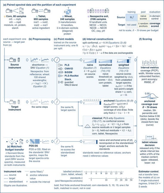
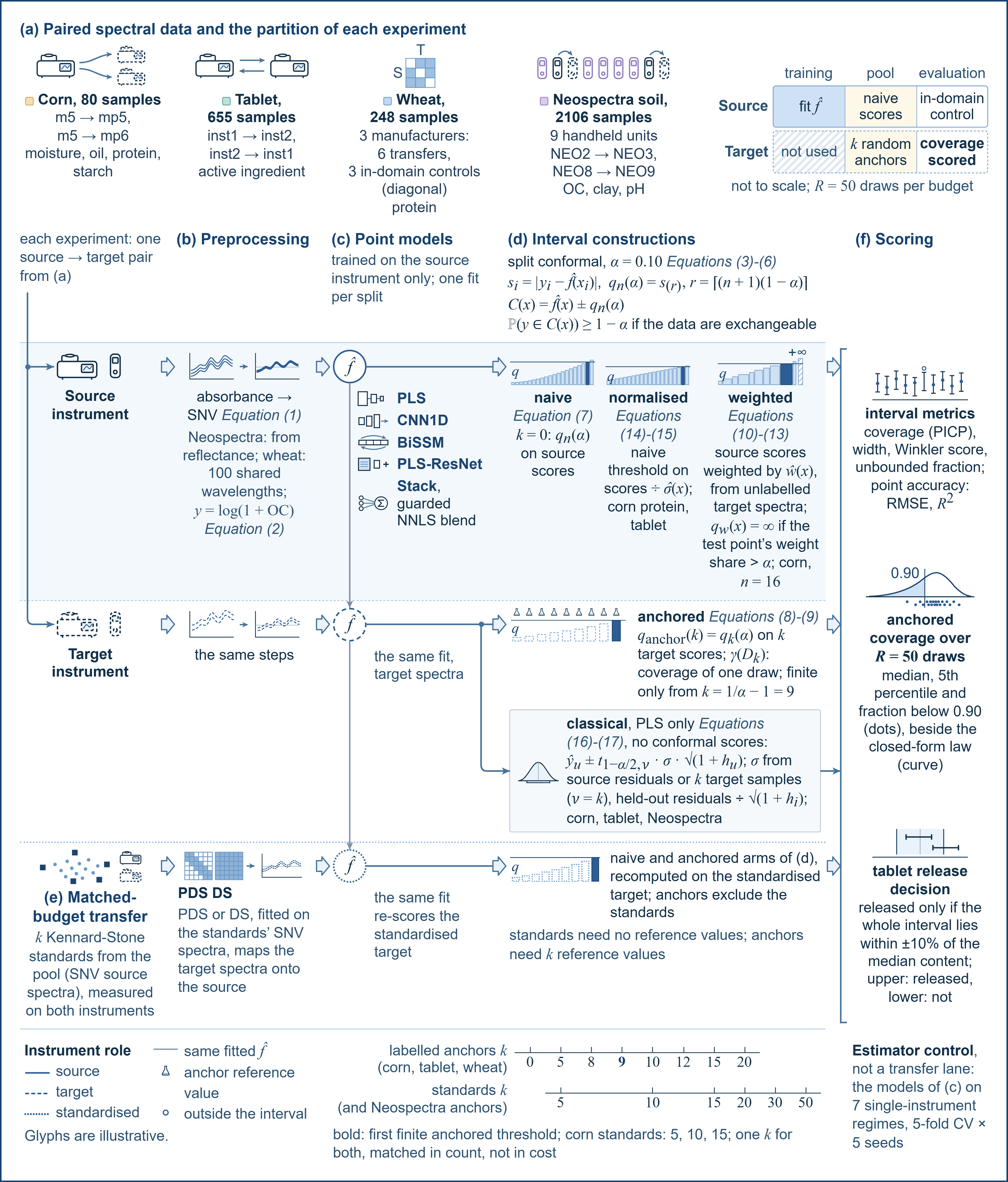
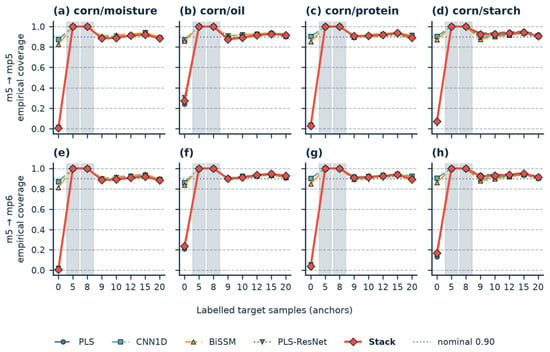
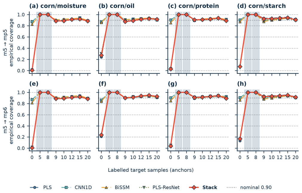
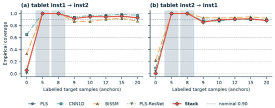
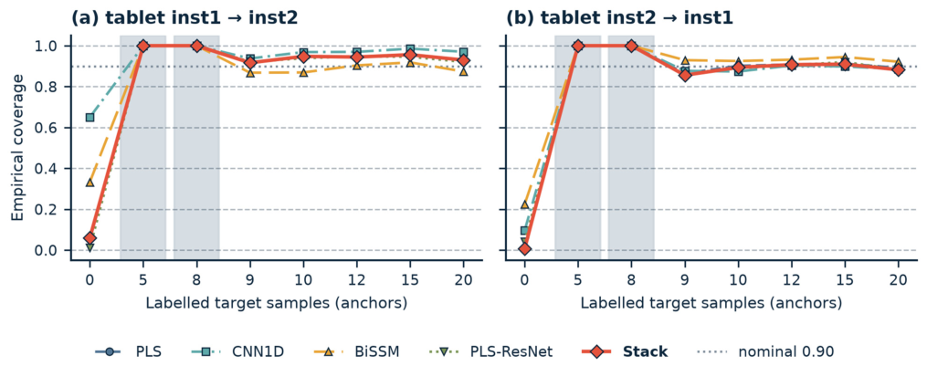
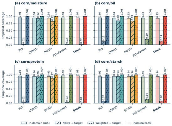
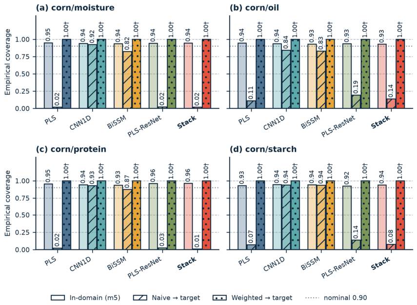
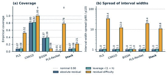
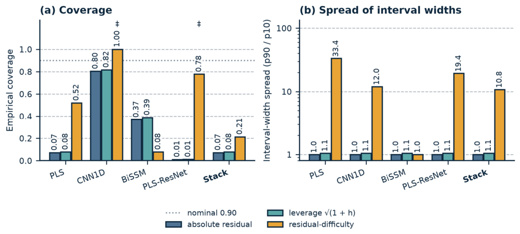
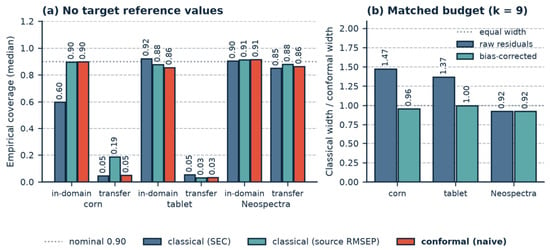
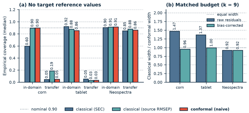
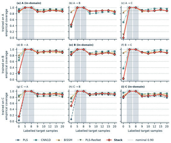
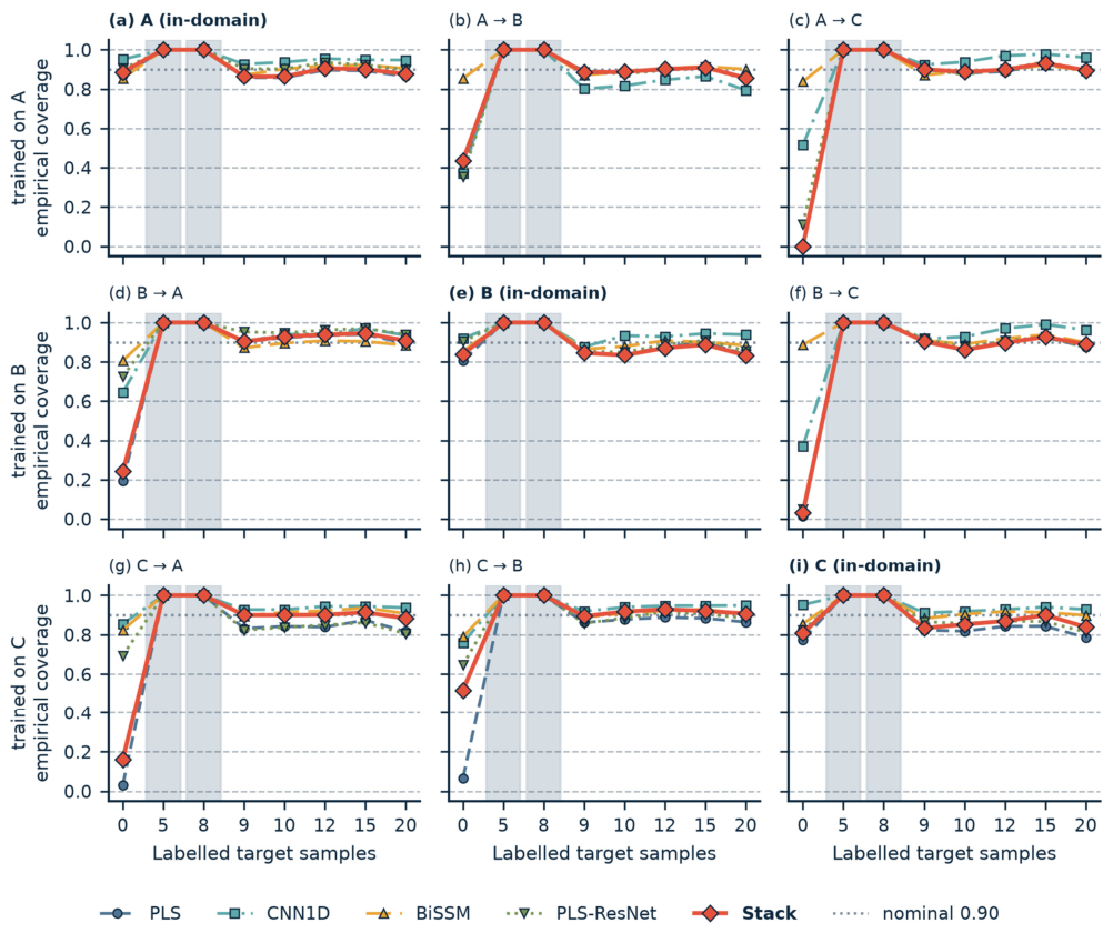
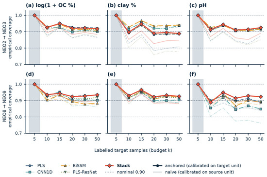
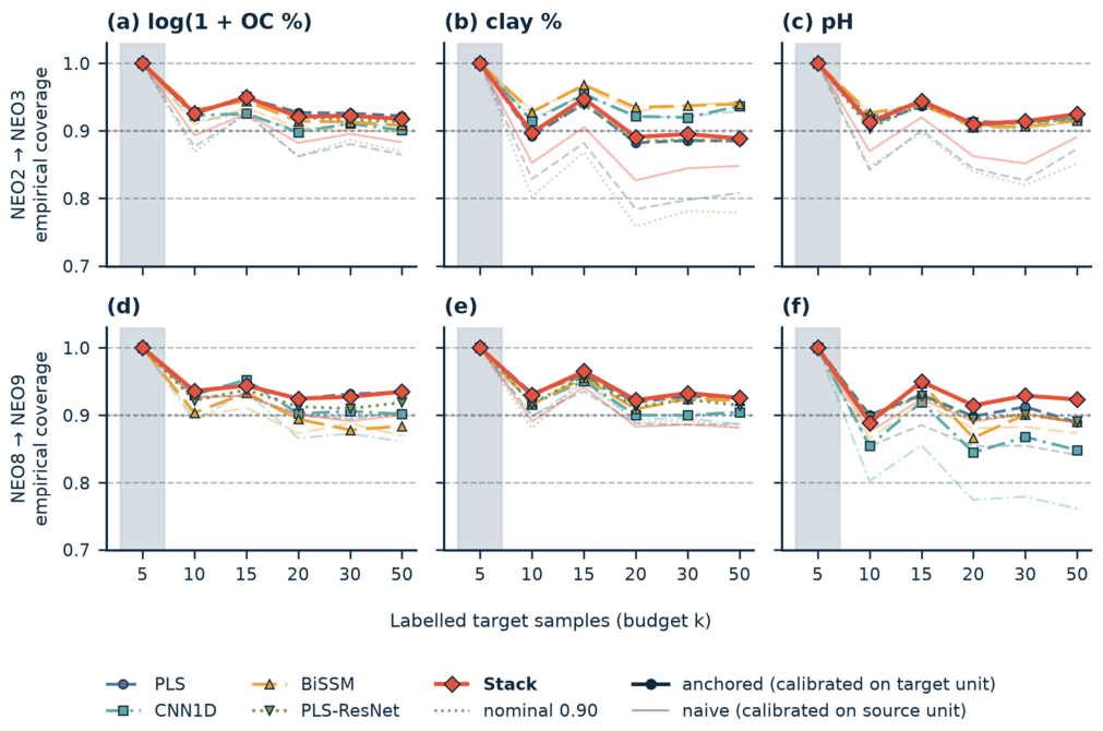
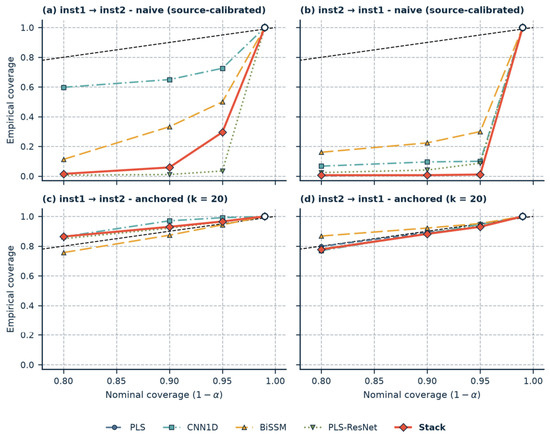
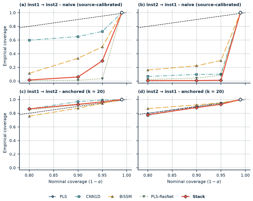
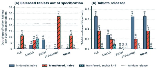
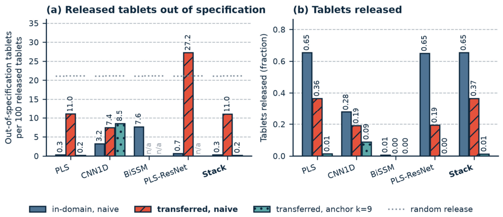
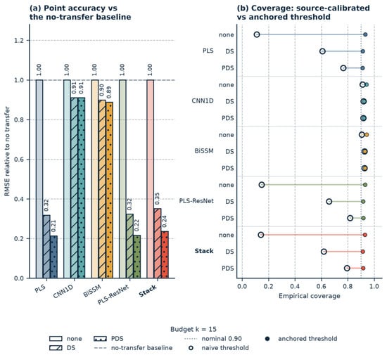
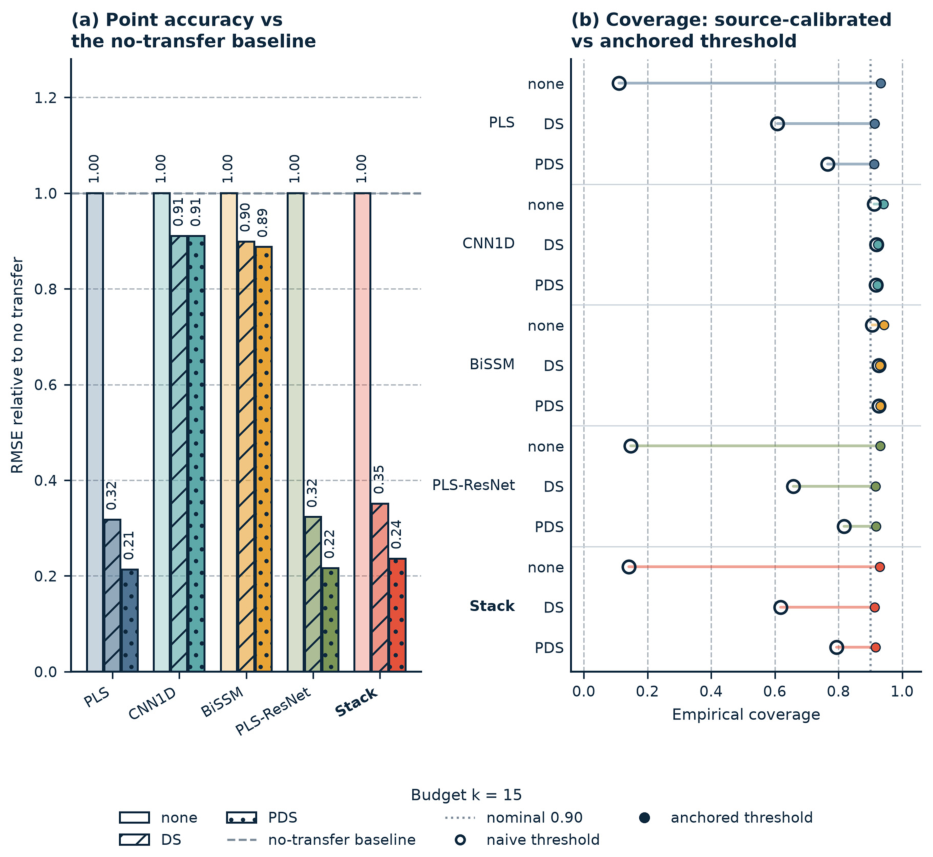
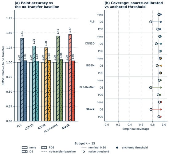
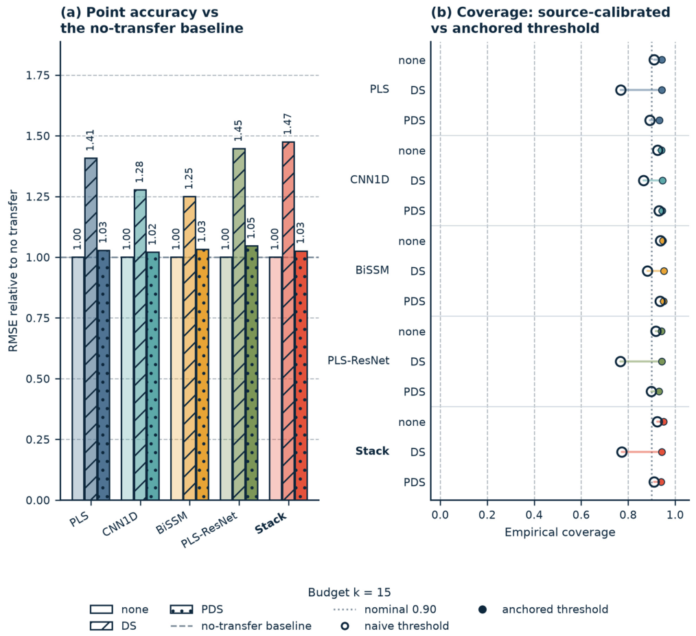

Disclaimer/Publisher’s Note: The statements, opinions and data contained in all publications are solely those of the individual author(s) and contributor(s) and not of MDPI and/or the editor(s). MDPI and/or the editor(s) disclaim responsibility for any injury to people or property resulting from any ideas, methods, instructions or products referred to in the content. |
© 2026 by the authors. Licensee MDPI, Basel, Switzerland. This article is an open access article distributed under the terms and conditions of the Creative Commons Attribution (CC BY) license.