


Featured Application
The proposed Knowledge-guided Hierarchical Constraint Co-Evolutionary Algorithm (KHCEA) is specifically designed for layout transformation and coordinated dispatch operations of Automated Guided Vehicle (AGV) fleets in restricted logistical spaces aboard large-scale surface transportation platforms, and is particularly applicable to scenarios involving high-density AGV parking, limited operational-area availability, tight turnaround schedules, and strongly coupled constraints. The KHCEA can be embedded as a decision support engine in platform-level logistics dispatching systems, providing real-time or near-real-time scheduling solutions for AGV parking position assignment, path selection, configuration transformation timing, and dispatch sequencing.
Abstract
The layout transformation and coordinated dispatching of Automated Guided Vehicles (AGVs) in restricted spaces constitute a critical link in improving the throughput efficiency of large-scale surface transportation platforms. Traditional scheduling algorithms struggle to effectively address large-scale optimization problems interwoven with multiple constraints, including configuration switching, spatial interference, and temporal coupling. To this end, this paper proposes a Knowledge-guided Hierarchical Constraint co-Evolutionary Algorithm (KHCEA). Taking the post-recovery transfer of AGV fleets from temporary parking positions to maintenance parking positions as a representative scenario, this study comprehensively considers decision elements such as AGV configuration transformation, parking position assignment, path selection, and start-time scheduling, and formulates a multi-objective nonlinear integer programming model. The model constraints are classified into four hierarchical levels according to their objects of action and computational characteristics, which are embedded into individual generation, fitness evaluation, directed mutation, and post-validation stages, respectively. A knowledge base mechanism is introduced to extract high-frequency gene patterns from historically superior solutions to guide mutation directions, while a Pareto non-dominated archive is maintained to coordinate multi-objective trade-offs. Simulation results demonstrate that KHCEA outperforms comparison algorithms in both solution accuracy and stability. For the 16-vehicle case, KHCEA reduces the normalized weighted objective value by 3.2% on average and the standard deviation of the results by 7.4% relative to the strongest comparison algorithm (the repair-enhanced DE-R); relative to the best classical baseline (DE), the corresponding reductions are 7.2% and 13.8%, confirming its satisfactory solution quality, stability, and practical applicability.
1. Introduction
As a cornerstone of modern maritime transportation, the operational effectiveness of large-scale surface transportation platforms is directly determined by the turnaround rate of Automated Guided Vehicles (AGVs), with dispatch and maintenance capabilities within restricted operational spaces constituting the critical upper-bound determinant [1]. Under high-intensity cyclic operating conditions, frequent folding and unfolding operations of lateral mechanisms not only intensify competition for spatial resources in the operational area but also accelerate fatigue wear of hydraulic servo systems and folding-locking mechanisms, thereby incurring unscheduled maintenance man-hours and impairing the sustained deployment capability and dispatch reliability of AGV fleets [2]. Consequently, conducting optimization research on layout transformation and coordinated dispatch scheduling for AGV fleets under restricted-space and complex fleet deployment constraints holds substantial theoretical value and engineering application significance for enhancing the operational efficiency of large-scale surface transportation platforms in extreme operating environments.
Under restricted-space and complex fleet dispatch constraints, the dispatch process of an AGV fleet transitioning from its initial layout state to a target layout state is inherently a systemic decision-making problem involving two interrelated layers: path planning and dispatch scheduling. Specifically, given the initial parking positions of the AGV fleet, the initial configuration of each AGV, and the set of available destination parking positions, it is necessary to coordinately determine the dispatch start time, configuration transformation scheme, travel path selection, and destination parking position assignment for each AGV, so as to achieve safe and efficient transfer of the AGV fleet within a finite spatial domain. In this framework, the path planning layer primarily addresses the geometric feasibility and dynamic executability of individual AGV motion trajectories, constituting the spatial foundation for dispatch safety; the spatial scheduling layer, in contrast, focuses on the temporal sequencing and resource allocation of multi-AGV operations, serving as the decision-making core for dispatch efficiency enhancement. These two layers are deeply intertwined through spatial occupancy and temporal coupling: path selection determines the spatial envelope of each AGV at any given moment, while the scheduling sequence must be coordinated under the prerequisite that the spatial envelopes of all AGVs remain mutually non-overlapping. Therefore, path planning and scheduling optimization must be unified within a holistic problem-solving framework for careful consideration.
(I) Path Planning
Single-AGV dispatch path planning requires the generation of collision-free feasible trajectories from the starting parking position to the destination parking position, given the known start and end positions and environmental obstacle distribution, while incorporating AGV kinematic and dynamic constraints [3,4,5]. To date, multiple technical approaches have been developed for single-AGV path planning. Early research was dominated by direct methods based on optimal control, formulating path planning as time-optimal or energy-optimal control problems solved via tools such as pseudospectral methods [4,6]. These approaches offer the advantage of handling kinematic constraints and terminal pose requirements within a unified framework, yet they are sensitive to initial guesses and prone to local optima in complex obstacle environments [3]. To overcome these limitations, researchers have integrated heuristic search with optimal control, giving rise to hybrid frameworks characterized by “global coarse planning + local refined optimization.” One line of work employs the A* algorithm to generate sequences of key path points, which are subsequently refined via optimal control [3]; another line utilizes closed-loop Rapidly Exploring Random Trees (RRT), combining the rapid exploration capability of sampling-based methods with the online optimization capability of Model Predictive Control (MPC) [7]. In recent years, a more systematic “search–resampling–optimization” three-layer framework has been proposed, which introduces the concept of safe dispatch corridors to simplify complex collision-avoidance constraints into corridor-internal constraints, thereby significantly enhancing computational efficiency and robustness in densely cluttered environments, with successful extensions to more complex application scenarios such as towing systems [8,9]. On this basis, Li et al. [10] further proposed an iterative safe dispatch corridor framework, which effectively improves the quality and computational efficiency of trajectory planning by iteratively refining the corridor constraints.
In scenarios where multiple AGVs share a restricted space, the simple superposition of individual AGV collision-free trajectories does not guarantee the overall safety of the AGV fleet; coordinated collision avoidance must be achieved through temporal coordination and trajectory selection among multiple AGVs [11,12]. Existing research primarily proceeds along two pathways: centralized and distributed. Centralized methods perform global optimization to plan coordinated trajectories for all AGVs uniformly, achieving theoretical optimality, but incurring computational burdens that escalate dramatically with problem scale [13]. Distributed methods, on the other hand, endow each AGV with a certain degree of autonomous decision-making capability, performing local adjustments through mechanisms such as dynamic prioritization or velocity obstacles, thereby offering favorable scalability and real-time performance [11,14,15,16]. Building upon this foundation, Xin et al. [17] formulated AGV fleet path planning as a mixed logical dynamical system and applied model-predictive, receding-horizon optimization with distributed coordination to generate conflict-free trajectories online, thereby validating the feasibility of integrating rolling-horizon optimization with distributed coordination for multi-AGV planning. More recently, deep reinforcement learning has demonstrated emerging application potential in path planning. Chen et al. [18] addressed the path planning problem for urban low-altitude unmanned aerial vehicles under noise-threshold constraints in residential areas, proposing the TNAP-DDQN algorithm with flight time and safety risk as optimization objectives. By introducing a noise-attenuation mask-based action bias network and prioritized experience replay, they achieved synergistic optimization of noise compliance and flight efficiency, offering a new paradigm for extending path planning from conventional obstacle avoidance to multi-dimensional constraint optimization.
In terms of solution methodologies, single-AGV path planning has evolved from purely optimal control toward hybrid frameworks. Liu et al. [5] proposed symplectic-conserving pseudospectral methods within a time–energy hybrid optimal control framework, and subsequently [4] integrated receding-horizon control to achieve high-precision online tracking. Han et al. [3] employed improved-A* waypoints with Radau pseudospectral segmented planning to reduce the dependence on initial guesses, while Wang et al. [8] proposed a “search–resampling–optimization” framework that decouples the problem scale from the number of obstacles and has been extended to towing systems [9].
In the domain of multi-AGV collaborative path planning, the research focus has gradually shifted from distributed coordination strategies toward deep integration of geometric collision-avoidance theory with optimal control. Wu et al. [11] proposed a distributed planning architecture with an asynchronous token-based strategy, effectively circumventing deadlock issues inherent in synchronous planning. Liu et al. [12] combined the Reciprocal Velocity Obstacle (RVO) method with Dubins curves and introduced the One-sided Symplectic Pseudospectral (OSSP) method for precise planning of terminal trajectory segments, achieving a balance between collaborative collision-avoidance efficiency and terminal constraint accuracy. Wang et al. [13] unified multi-AGV collaborative taxiing within an optimal control framework, employing Dubins curves to provide high-quality initial solutions and integrating MPC to realize unified centralized planning with distributed tracking. In the broader context of general AGV fleet operations, integrated mission design and fleet-level motion planning have also been extensively investigated: Xidias and Azariadis [19] addressed mission design for a group of autonomous guided vehicles, and subsequently proposed a method for computing collision-free motions for a team of robots under formation and non-holonomic constraints [20], providing important foundations for fleet-level cooperative planning. A summary of the relevant literature is provided in Table 1.
Table 1.
Summary of path planning research.
(II) Dispatch in Restricted Spaces
The layout transformation and coordinated dispatch scheduling of AGV fleets in restricted spaces constitute a class of combinatorial optimization problems characterized by strong coupling across the three dimensions of time, space, and resources. The decision-making process encompasses dispatch sequencing, parking position assignment, configuration transformation selection, and personnel–equipment coordination. Configuration transformations directly alter the availability status of parking positions on the operational area; temporal conflicts among parking positions constrain dispatch windows; and path interference coupled with resource limitations further compresses scheduling flexibility. The constraint structure of this problem is large in scale and exhibits hierarchical and conflict-propagation characteristics: a violation of a single constraint may result from the combined effect of multiple decision variables, while local rectification may trigger renewed violations of other constraints. Traditional scheduling methods prove inadequate in such strongly coupled structures: exact solution algorithms become incapable of identifying feasible solutions within reasonable time as problem scale expands, while conventional metaheuristic algorithms often exhibit slow convergence, considerable variability in solution quality, and frequent failure to generate fully constraint-satisfying schedules when confronted with strongly coupled constraints. The following paragraphs review relevant research progress from the perspective of operational area dispatch.
In terms of model formulation, early studies predominantly adopted the hybrid flow shop or Flexible Job Shop Scheduling Problem (FJSP) framework, treating AGVs as jobs and operations as fixed processing flows, with the objective of minimizing makespan [21]. As understanding of actual operational processes deepened, researchers gradually recognized that the precedence dependencies involved in spatial dispatch are not linear chains but rather exhibit network-like, multi-resource-coupled characteristics. A single shop-scheduling model proved inadequate for accurately characterizing the complex temporal relationships of maintenance operations. Consequently, the field introduced a series of models based on the Resource-Constrained Project Scheduling Problem (RCPSP), treating the maintenance operations of each AGV as a project, describing the partial order relationships among operations through network-based models, and incorporating multiple constraint categories—including personnel, equipment, workstation space, and supply resources—within a unified framework [22]. Concurrently, the research perspective has expanded from scheduling optimization under given resource conditions to joint optimization of schedules and resource allocation, revealing the marginal effects between resource increments and completion time [23].
In terms of solution methodologies, given the NP-hard nature of the problem, researchers first attempted exact methods such as Mixed-Integer Linear Programming (MILP), yet such approaches can only obtain optimal solutions for small-scale problems and prove inadequate for practical scheduling scenarios [24]. Subsequently, solution methodologies have evolved along two primary technical pathways. The first pathway centers on single-solution iterative optimization with Adaptive Large Neighborhood Search (ALNS) as the core, wherein methods iteratively improve from an initial solution through ruin-and-recreate neighborhood operations. Balouka and Cohen [23] addressed the multi-mode resource-constrained project scheduling problem through robust optimization, in which activity execution modes jointly determine the schedule and the resource configuration, thereby coordinating scheduling with resource allocation. However, the ALNS framework struggles to maintain temporal consistency across stages and global configuration–space–time consistency under scenarios with multi-stage operational continuity and cross-stage resource dependencies. The second pathway features metaheuristic algorithms represented by Genetic Algorithms (GA), which have gradually become mainstream solution approaches by virtue of their favorable global search capability and problem adaptability [22,25]. Neufeld et al. [26] systematically reviewed multi-objective hybrid flow shop scheduling, a model class that has been widely adopted to model full-process scheduling with multiple coupled stages. Singh et al. [27] developed a matheuristic for scheduling heterogeneous AGV fleets with battery constraints, tackling AGV deployment scheduling under resource and time-window requirements. Nevertheless, standard GA and its variants typically incorporate constraints into the fitness function as penalty terms, lacking deep exploitation of the problem’s structural characteristics. When confronted with dynamic spatial constraints driven by configuration transformations, they are unable to proactively maintain solution feasibility during evolution, expending substantial computational resources on screening and repairing infeasible solutions. More recently, Song et al. [28] modeled flexible job-shop scheduling as a sequential decision process and learned high-quality dispatching policies through deep reinforcement learning with graph neural network representations, thereby validating the feasibility of deep reinforcement learning for real-time scheduling. The models and solution methodologies of the above representative studies are summarized in Table 2.
Table 2.
Summary of the spatial dispatch literature.
Despite the notable progress achieved by the above studies in both model accuracy and solution efficiency, existing research on spatial dispatch still suffers from two deficiencies. First, existing algorithms struggle to balance the strongly coupled constraints within limited spatial domains against multi-objective optimization requirements. Single-solution iterative methods are prone to becoming trapped in local optima during multi-objective trade-offs, while population-based evolutionary methods encounter difficulties in configuring parameter weights, often resulting in excessive suppression of certain sub-objectives. Within finite computational windows, algorithms find it challenging to simultaneously achieve computational efficiency and satisfactory optimization quality, rendering the resulting schedules insufficiently feasible for engineering implementation. Second, although AGV configuration serves as an active variable for regulating the utilization efficiency of restricted space, current research predominantly treats it as either a fixed input or a post hoc adjustment measure, without incorporating it as an endogenous decision variable within the scheduling process. Consequently, scheduling schemes lack the flexibility to resolve conflicts through proactive configuration transformation when spatial conditions tighten. Deng et al. [29] indirectly incorporated configuration differences into the scheduling framework through parking position type selection; however, the timing of configuration transformations remains predetermined prior to dispatch initiation and has not achieved online coordination with dispatch sequencing.
To address the above limitations, this paper introduces targeted improvements at three levels within the co-evolutionary algorithm framework. (1) At the operator level, hard constraint handling is embedded into the selection and mutation operators, internalizing constraint satisfaction as an inherent property rather than an external penalty, ensuring global configuration–space–time consistency throughout evolution. (2) At the architecture level, a three-layer sub-population co-evolutionary architecture is established. To address “information deadlock” in co-evolution, probabilistic fixed-partner and joint mutation mechanisms are introduced to break stagnation caused by information isolation among sub-populations. (3) At the guidance level, a knowledge-base-driven directed mutation mechanism is constructed, which leverages historical data and empirical knowledge to guide the search process of traditional optimization algorithms [30], thereby reducing ineffective exploration and accelerating convergence. These enhancements enable the algorithm, while preserving the generality of population-based evolution, to deeply adapt to the structural characteristics of the layout transformation and dispatch scheduling problem [31].
The remainder of this paper is organized as follows. Section 2 provides a formal description of the AGV fleet layout transformation and coordinated dispatch problem, including the problem background and problem definition. Section 3 establishes the mathematical model for AGV fleet transfer and layout, covering model assumptions, parameter definitions, decision variables, constraints, and objective functions. Section 4 presents the proposed KHCEA in detail, including the hierarchical constraint internalization framework, the three-population architecture, the encoding mechanism, knowledge-guided rules, and evolutionary operators. Section 5 describes the simulation setup and reports experimental results, covering hyperparameter analysis, algorithm comparison, and ablation experiments. Section 6 presents the discussion, and Section 7 concludes the paper.
2. Problem Description
2.1. Problem Background
The layout transformation of AGVs in restricted spaces runs through all stages of AGV lifecycle maintenance and connects hangar storage, operational area maintenance, and vehicle movement. It primarily covers three scenarios: deployment maintenance, post-recovery re-layout, and recovery maintenance/parking. Although these scenarios differ in origins, destinations, and operational objectives, their decision-making essence is consistent: under restricted-space resource constraints, the configuration transition scheme, destination parking position assignment, dispatch path selection, and dispatch start time of each AGV must be jointly optimized to achieve an efficient and orderly fleet transfer under safety constraints.
In the large-scale surface transportation platform application scenario considered in this paper, the term ‘AGV’ generally refers to aircraft or large mobile equipment deployed within the platform’s operational area. Since such equipment has no autonomous power when undergoing layout transformation in restricted spaces, it must be towed by a dedicated towing device. To maintain consistency with the standard terminology of the scheduling community, this paper abstracts the ‘aircraft–towing-device combination’ as a single AGV task subject to mathematical modeling and algorithmic solution, whose kinematic parameters (upper bounds of velocity and acceleration) are taken from those of the towing combination; the specific parameter settings are given in Section 5.1. Accordingly, “AGV dispatch” throughout this paper refers to the movement of the aircraft–towing combination. Although the proposed method is motivated by this scenario, it can be generalized to other integrated AGV fleet planning problems with configuration-transformation requirements.
The four towing devices equipped in the operational area are characterized in the mathematical model through constraint C6 as an upper bound on the number of transfer tasks that can be executed simultaneously, while the specific assignment of towing devices is completed at the scheme concretization stage. In the order of task start times, the system sequentially assigns to each task the idle towing device nearest to its starting point, and during the operation the towing device moves integrally with the mobile combination. Since constraint C6 strictly limits the number of concurrent tasks to no more than the total number of towing devices, at any moment, whenever a towing demand for task execution arises, a released idle towing device is necessarily available. Assuming that deadhead transfer time is not counted in the scheduling duration, the tug assignment adopts a nearest-dispatch strategy aimed at minimizing the physical deadhead distance of towing devices between adjacent tasks. This concretized assignment serves only as a mapping for the physical execution of the dispatch scheme and does not alter the operational sequence or the concurrency upper bound determined on the original scheduling timeline.
This paper takes the post-recovery re-layout phase as the representative research object, focusing on transferring the AGV fleet from temporary parking positions to maintenance parking positions after mission completion. The key decisions involve dispatch sequencing, spatial occupancy coordination, and resource conflict resolution. The proposed modeling and algorithmic framework can be extended to the other two phases by adjusting the mapping relationships among parking position sets and the corresponding spatial constraints.
2.2. Problem Definition
Given a set of AGVs with known initial parking positions and initial configurations, all AGVs must be transferred to available parking positions in the maintenance area. The spatial distribution and availability of parking positions are known a priori, while the destination parking position of each AGV is determined by decision-making. An AGV initially in the spread configuration may switch to the folded configuration to reduce its footprint, whereas an AGV initially folded undergoes no configuration transformation. Each AGV travels along a preset feasible path from its initial position to its destination, with the path selected from a pre-constructed path library that already satisfies single-AGV kinematic constraints and static obstacle avoidance requirements.
Because the physical dimensions of AGVs differ significantly between spread and folded configurations, the same physical location is defined as independent logical parking positions under the two configurations. The operational area is functionally divided into a temporary area and a maintenance area. In the temporary area, all AGVs are initially parked in the spread configuration at fixed positions, and the spread and folded parking positions fully overlap in physical location; after configuration transformation, the logical parking position index changes while the physical location remains unchanged. In the maintenance area, spread and folded parking positions are independently arranged in a staggered layout and only partially overlap, as shown in Figure 1.
Figure 1.
Dispatch area functional zoning.
The core of the decision-making process lies in jointly determining three interrelated elements for each AGV: (1) the destination parking position, which implicitly determines the final configuration state; (2) the dispatch path selected from the path library; and (3) the dispatch start time in discrete time steps. These three decision variables are mutually coupled and collectively constitute a complete transfer scheduling scheme for the AGV fleet.
In determining these decisions, a series of complex constraints must be satisfied, covering resource allocation, concurrent operation restrictions, logical temporal relationships, and dynamic safety collision avoidance, which exhibit notable hierarchical and coupling characteristics. Scheme quality is evaluated by three objectives aggregated via priority-weighted summation: the number of configuration changes as the primary objective, the total dispatch time as the secondary objective, and the total path length as the tertiary objective. Accordingly, the core difficulties lie in three aspects: the strong coupling among configuration, space, and timing; the mixed discrete-continuous decision space; and the hierarchical nature of constraints with conflict propagation characteristics.
3. AGV Fleet Transfer and Layout Model
3.1. Model Assumptions
1. The layout of the operational space is assumed to remain unchanged throughout the entire scheduling horizon, with no new obstacles or temporary zones emerging.
2. The dispatch process is assumed to be discrete in time, divided by a fixed time step △t. The discrete temporal resolution is assumed to be sufficient to fully capture the state transitions of the scheduling process.
3. The time consumed by configuration transformation is not directly accounted for in the dispatch duration; rather, its cost is indirectly reflected through the optimization objectives.
Regarding the timing of configuration transformation, the following rule is adopted in this paper. When an AGV needs to perform a configuration transformation, if it switches from the spread configuration to the folded configuration, the transformation is completed before dispatch begins at its initial temporary parking position; if it switches from the folded configuration to the spread configuration, the transformation is performed after it arrives at the destination parking position. In both cases, the configuration transformation does not occupy dispatch time and therefore introduces no additional collision-avoidance computational burden.
4. Each AGV performs exactly one dispatch task from its temporary parking position to a maintenance parking position, and once initiated, the task proceeds without interruption until completion.
5. The deadhead transfer of towing devices between tasks is not counted in the scheduling duration; the assignment of towing devices is completed at the scheme concretization stage following deterministic rules and does not affect the scheduling decision variables.
3.2. Parameter Definitions
The parameters involved in the AGV fleet transfer and layout model are defined in Table 3. The units of all physical quantities follow the SI system; time-related symbols are expressed in seconds (s) and length-related symbols in meters (m), while count-type and 0–1 indicator symbols are dimensionless.
Table 3.
Parameter definitions.
3.3. Decision Variables
According to the problem definition and parameter system established above, the decision variables of the proposed model are summarized in Table 4.
Table 4.
Decision variables.
ei is not an independent decision variable but is uniquely determined by the assignment variables xikp. A folded parking position occupies less platform area than a spread one; therefore, when the operational space cannot accommodate all AGVs in the spread configuration, some AGVs are assigned to folded parking positions to release platform space, and the configuration state of each AGV is thus coupled to the final fleet layout. Formally, .
3.4. Constraints
A. Task Assignment and Fundamental Definition Constraints
(1) Uniqueness constraints for assignment and path
Each AGV must be assigned to exactly one parking position and must select exactly one path.
(2) Folded AGV configuration invariance
All AGVs with ci = 0 cannot be assigned to any spread-configuration parking position.
(3) Association constraint between task assignment and start time
If AGV i is assigned a task, it has exactly one start time.
B. Resource Capacity Constraints
(4) Parking position capacity constraint
Each parking position can accommodate at most one AGV.
(5) Total parking position capacity constraints for the operational area
(6) Constraint on the number of AGVs that can be dispatched simultaneously in the operational area
Due to resource constraints such as the limited number of tow tractors, the number of AGVs that can be dispatched simultaneously within a single time step is restricted, where Nmax is set to the number of available tow tractors.
C. State Association Constraints
(7) Relationship between parking position occupancy and AGV assignment
(8) Activation condition for arrival dispatch conflict groups
where |•| denotes the number of parking positions contained in •.
D. Spatiotemporal Conflict Constraints
(9) Spatial interference constraint for maintenance parking positions
If interference exists between a spread parking position and a folded parking position, i.e., Muv = 1, then they cannot be occupied simultaneously; that is, parking positions u and v cannot simultaneously accommodate two AGVs.
(10) Collision-avoidance constraint during the dispatch process
Let the spatial envelopes of any two AGVs i,j at time step t be denoted as Vi,Vj. The collision-avoidance constraint is then expressed as
(11) Temporal sequencing constraint for arrival dispatch conflicts
The completion time of any dispatch task must be earlier than the completion times of all other tasks that occupy its arrival path.
Suppose AGV i is assigned to parking position k1 ∈ Ag, AGV j is assigned to parking position k2 ∈ Cg, with dispatch start times t1 and t2, and selected paths p1 and p2, respectively. The arrival constraint is then expressed as
(12) Temporal sequencing constraint for departure dispatch conflicts
If the parking position of one AGV occupies the departure path of another, the obstructing AGV must start its transfer first; equivalently, the start time of any dispatch task must be later than the start time of the task occupying its path.
Suppose AGV i is assigned to parking position k1 ∈ Eb, AGV j is assigned to parking position k2 ∈ Db, with dispatch start times t1 and t2, and selected paths p1 and p2, respectively.
3.5. Objective Functions
For the AGV fleet transfer problem, three optimization objectives—the number of configuration changes, the total dispatch time, and the total path length—are constructed, with balancing weight coefficients assigned to each. The number of configuration changes affects equipment service life and maintenance efficiency and is set as the primary objective; the total dispatch time F2 = T is the core indicator influencing the sortie rate and is set as the secondary objective; the total path length is the tertiary objective, used to further screen schemes with better energy consumption when the first two objectives are comparable. The total transfer time is defined as
Since the three sub-objectives differ in dimension and order of magnitude, they are aggregated in the algorithm through search weights acting on the raw sub-objective values, so that the search cost is expressed in the original dimensions as
where , and are used to construct the fitness in the evolutionary search, with the constraint-violation penalty term embedded in the fitness evaluation stage. The fitness used internally by the evolutionary search for selection operations is defined as the search-layer fitness, i.e., the sum of the priority-weighted cost aggregated by the search weights and the constraint-violation penalty term, and is used solely for elite retention and tournament selection within the algorithm.
For scheme evaluation and cross-algorithm comparison, a separate set of comparison weights is adopted. Before the weighted aggregation, each sub-objective is divided by its normalization reference value Ni (i = 1,2,3, corresponding to the number of configuration changes, the total dispatch time, and the total path length, respectively) to obtain dimensionless normalized sub-objectives. The reference value Ni is determined based on statistical results from typical scenarios and theoretical lower bounds, so that the normalized values of the sub-objectives fall within a comparable range. The normalized weighted objective is expressed as
The comparison weights Wc are introduced for two purposes. First, they provide a unified metric for cross-algorithm comparison. Second, they serve as the decision criterion for selecting the final scheme from the Pareto archive. When the algorithm terminates, all solutions in the external archive are feasible solutions with zero penalty, and their normalized weighted objective values Zc are used for scheme evaluation and cross-algorithm comparison.
4. Knowledge-Guided Hierarchical Constraint Co-Evolutionary Algorithm
To address the diverse and tightly coupled constraint types characterizing the optimization model established above, this chapter proposes a Knowledge-guided Hierarchical Constraint Co-Evolutionary Algorithm (KHCEA). The algorithm adopts a hybrid strategy of hierarchical constraint internalization and multi-population co-evolution, embedding learning mechanisms into the traditional evolutionary framework to enhance constraint handling and collaborative optimization capabilities [32]. Compared with existing techniques, the innovative increments of KHCEA are threefold. First, unlike conventional co-evolutionary algorithms, in which sub-populations interact mainly through representative exchange, KHCEA couples its three sub-populations with an explicit knowledge model that is statistically extracted online from the Pareto archive and fed back into the mutation operators, so that accumulated search experience directly steers offspring generation. Second, unlike constraint-handling strategies that uniformly penalize or post-repair violations, the 12 constraints are classified into four hierarchical levels—encoding level, fitness level, mutation level, and validation level—according to their physical characteristics and computational complexity, and are respectively embedded into the encoding initialization, fitness evaluation, mutation operation, and post-validation repair stages, thereby transforming constraint handling from external penalty imposition to internally guided enforcement. Third, unlike trajectory-planning-based scheduling schemes in which path-library selection is decoupled from fleet-level scheduling, a three-population co-evolutionary architecture is constructed for parking position assignment, path selection, and temporal scheduling, enabling information exchange among decision variables through an optimal-representative transmission mechanism and jointly optimizing the three decision layers under layout transformation. A knowledge base guidance mechanism and a Pareto non-dominated sorting strategy are further introduced to direct the search using high-frequency patterns extracted from historically superior solutions, while an external archive is maintained to preserve the multi-objective frontier. The overall algorithm structure is illustrated in Figure 2.
Figure 2.
Algorithm architecture overview.
4.1. Hierarchical Constraint Internalization Framework
The optimization model established in Section 3 encompasses a total of 12 constraints (denoted as C1–C12), covering multiple aspects including resource allocation, spatial interference, temporal logic, and dynamic collision avoidance. These constraints exhibit significant differences in both physical semantics and mathematical structures. If a uniform treatment approach were adopted—whether imposing all constraints as fitness penalties or relying entirely on post hoc repair—it would be difficult to accommodate the inherent characteristics of each constraint type, leading to degraded search efficiency or compromised solution quality. Therefore, it is necessary to systematically classify the constraints according to their distinct properties and design tailored handling mechanisms for each category.
Standard GA typically incorporates all constraints uniformly into the fitness function as penalty terms, or performs centralized repair after evolution concludes. This externalized treatment suffers from two inherent deficiencies. First, different constraint types affect decision variables through distinct pathways; uniform treatment fails to reflect the internal structural differences among constraints, resulting in low search efficiency. Second, the repair process often disrupts the favorable genetic patterns accumulated within chromosomes during evolution, thereby impairing the algorithm’s convergence performance.
To address the above issues, this paper establishes a four-tier constraint internalization framework that decouples the 12 constraints and embeds them into distinct stages of the evolutionary algorithm. The classification criteria and specific partitioning of each tier are detailed in Section 4.1.1.
4.1.1. Constraint Classification and Hierarchical Strategy
Based on the types of decision variables on which constraints operate, their degrees of mandatory enforcement, coupling scopes, and computational complexities, the 12 constraints are partitioned into four hierarchical levels, as presented in Table 5.
Table 5.
Hierarchical classification of constraints.
Tier 1 comprises encoding-level hard constraints (C1–C5, C7–C9), which pertain to the legality of individual decision variables and the fundamental correspondences among AGVs. These are implemented through encoding structure design and generation-time validation, ensuring that the individuals participating in evolution satisfy the basic physical and resource constraints. Details of implementation are provided in Section 4.2.1.
Tier 2 consists of the fitness-level soft constraint (C6), whose satisfaction depends on the joint distribution of the start times of all AGVs. It is implemented by imposing penalties on chromosomes that violate the constraint.
Tier 3 encompasses mutation-level temporal constraints (C11 and C12), which describe the precedence relationships among AGV dispatch operations. If these constraints were treated merely as fitness penalty terms, the algorithm would only obtain binary feedback indicating violation or compliance, providing little effective guidance for adjusting the temporal variables. Through directed mutation operators that directly adjust start times to eliminate conflicts, constraint repair can be incorporated as an organic component of the search process. Implementation details are presented in Section 4.3.3.
Tier 4 comprises the validation-level dynamic collision-avoidance constraint (C10). Since it requires determining the geometric overlap of motion envelopes between any pair of AGVs in the continuous spatiotemporal domain, its computational cost far exceeds that of the first three tiers. It is therefore designated for centralized validation and repair in the later stages of evolution. Implementation details are provided in Section 4.3.3.
The four tiers of constraints are embedded into the encoding, fitness, mutation, and validation stages according to their respective characteristics, forming a constraint-internalized processing system that spans the entire evolutionary process. To steer the algorithm toward constraint-satisfying regions during execution, penalty values are assigned to each constraint category, and penalty coefficients are set according to the severity of violation, so as to ensure that constraint-violating individuals are consistently inferior to feasible individuals in terms of fitness. The specific values are given in Table 6. As evolution proceeds and the hierarchical mechanism continuously repairs violations, the penalty terms of individuals in both the population and the external archive gradually approach zero, so that the penalty terms affect only the search trajectory rather than the evaluation of the final solution.
Table 6.
Penalty coefficient settings for each constraint.
4.1.2. Three-Population Collaborative Architecture
Building upon the hierarchical constraint classification, the algorithm partitions the population into three independent sub-populations according to decision variable types, corresponding respectively to parking position assignment, path selection, and temporal scheduling. These three categories belong to discrete combinatorial, discrete selectional, and discrete sequential decision spaces, respectively. If a unified chromosome encoding were adopted, crossover and mutation operations would readily disrupt the coordination among variables, leading to an elevated proportion of infeasible solutions and compromised search efficiency. To this end, the three variable types are encoded separately into three sub-populations, each executing genetic operations independently while achieving collaborative optimization of the overall solution through information exchange. The three-population architecture supports the design of differentiated operators tailored to each variable type, while decomposing the original high-dimensional decision space into three lower-dimensional subspaces, thereby reducing search difficulty.
Sub-population A is responsible for parking position assignment, with individuals represented as N-dimensional integer vectors, where the component i denotes the destination parking position index assigned to AGV i. Sub-population B is responsible for path selection, with individuals represented as N-dimensional integer vectors, where the i-th component denotes the relative index within the available path set of the current origin–destination pair, rather than the absolute ID in the global path library. When the complete chromosome is assembled for evaluation, this index is dynamically mapped to the corresponding available path set Pk according to the current destination parking position determined by sub-population A. Sub-population C manages temporal scheduling, with individuals represented as N-dimensional integer vectors, where the component i denotes the dispatch start time step of AGV i.
The three sub-populations achieve coordination through an “optimal-representative transmission” mechanism. When evaluating an individual in sub-population A representing a parking position assignment scheme, the path and timing information are supplemented by the current optimal individuals from sub-populations B and C, respectively, to assemble a complete chromosome for fitness computation. The evaluation of sub-populations B and C follows the same procedure. This mechanism ensures that the evolutionary direction of each sub-population is simultaneously guided by the quality of its own decision variables and the current best solutions of the other two tiers.
In terms of evolutionary sequence, a serial alternating strategy is adopted: within each generation, sub-populations A, B, and C sequentially complete selection, crossover, and mutation operations, and after each tier completes evolution, its optimal individual is updated for subsequent tiers’ evaluation. The primary direction of information flow is parking position assignment → path selection → temporal scheduling. Once parking position assignment is determined, the feasible set for path selection is consequently established, upon which temporal scheduling further optimizes the sequencing arrangements. This sequence aligns with the natural logic of the decision-making process, avoiding ineffective feedback from lower-level decisions to upper-level decisions. A schematic diagram of the three-population collaborative architecture is shown in Figure 3.
Figure 3.
Schematic diagram of the three-population collaborative architecture.
4.2. Encoding Mechanism and Knowledge-Guided Rules
Building upon the constraint hierarchical framework and the three-population collaborative architecture established in Section 4.1, this section elaborates on the specific implementation mechanisms of constraints at each level within encoding and genetic operations.
Given the multi-decision characteristics of the AGV layout transformation problem in restricted spaces, this paper adopts a three-layer parallel encoding structure that directly maps the three categories of decision variables onto independent chromosome genes. Each chromosome represents a complete operational area transfer scheduling scheme, expressed as an N × 3 integer matrix C, where N is the total number of AGVs, each row corresponds to one AGV, and the three columns respectively denote the destination parking position index k, the path index p, and the dispatch start time step τ:
4.2.1. Hard Constraint Encoding Implementation
The encoding-level hard constraints comprise eight in total (C1–C5, C7–C9), and their handling embeds legality validation logic into chromosome generation and genetic operations, ensuring that the generated individuals naturally satisfy the constraints without requiring subsequent repair or penalization. The specific handling mechanisms for each constraint are presented in Table 7. Among these, C1 and C4 are guaranteed by the chromosome structure design; C2, C5, and C9 are handled during the parking position assignment stage; C3 is handled during the time-step assignment stage; C8 is handled during the scheme assembly stage; and C7 is already satisfied when the chromosome is constructed, thus requiring no additional operations.
Table 7.
Implementation of hard constraints at the encoding level.
Through the above implementation mechanisms of encoding-level hard constraints, the legality concerning parking position assignment and time step assignment is guaranteed at the individual generation stage, obviating the need for re-validation during fitness evaluation or subsequent evolutionary stages. Individuals that fail to generate a legal chromosome during initialization due to an empty candidate set are directly discarded and regenerated until the population reaches the preset size.
4.2.2. Knowledge Base Construction and Guidance Rules
Although the above hard-constraint encoding ensures individual legality, the selection of candidate parking positions is still based on uniform random sampling and does not exploit the information of superior solutions accumulated during population evolution. As iterations proceed, individuals with higher fitness often exhibit recurring high-frequency patterns in parking position combinations and timing arrangements. If such patterns can be recorded and fed back into the subsequent search, blind exploration can be further reduced while satisfying the hard constraints. To this end, this section establishes a knowledge base construction and guidance mechanism, whose structure is illustrated in Figure 4.
Figure 4.
Schematic diagram of knowledge base construction and application.
As shown in Figure 4, the knowledge source of the knowledge base is the Pareto archive. Every 10 generations, the algorithm extracts superior individuals from the archive and statistically analyzes three categories of high-frequency patterns. The first category comprises parking position co-occurrence patterns, reflecting combinations of parking positions that frequently appear together within the same scheme. The second category consists of AGV–parking position assignment preferences, indicating which parking positions a specific AGV tends to be assigned to. The third category encompasses start-time distribution patterns, reflecting the relative intervals among the start times of AGVs in superior schemes. When the occurrence frequency of a pattern exceeds the threshold pm, it is stored in the knowledge base as a knowledge entry. The knowledge base capacity is capped at 100 entries, with updates governed by a First-In-First-Out (FIFO) policy. Path selection is temporarily excluded from knowledge guidance, as it is strongly coupled with parking position assignment; extracting path patterns independently would likely produce infeasible combinations, and introducing such knowledge would instead increase repair overhead. In each extraction round, all non-dominated solutions currently in the archive are taken as the statistical sample; the frequency of a pattern is defined as the proportion of sampled solutions containing it, and only patterns whose proportion exceeds the threshold (set to 0.3 in this paper) are admitted into the knowledge base as entries.
Knowledge guidance plays a role in both the initialization and mutation stages. When generating parking position assignment schemes during initialization, and when performing parking position or start-time substitutions during mutation, the algorithm reads the corresponding knowledge from the knowledge base for directed guidance with probability θ, and performs random selection within the legal range with probability 1 − θ. All individuals generated with knowledge guidance remain subject to the hard-constraint validation described in Section 4.2.1. In the initial evolutionary stage, the knowledge base is empty; the knowledge-guidance operations in initialization and mutation then automatically degenerate into uniform random selection within the legal range, without affecting individual feasibility, and knowledge guidance is enabled only after the Pareto archive has been sufficiently populated.
The knowledge base is updated online, with knowledge extraction and merging operations performed every 10 generations. Newly extracted knowledge entries are merged with existing entries in the base, and their frequencies are updated. If the number of entries exceeds the capacity limit, the earliest-entered entries are eliminated according to the FIFO rule. In the early evolutionary stages (first 20 generations), when the Pareto archive is insufficiently populated, no knowledge extraction is performed; thereafter, updates are conducted at fixed intervals. Each knowledge entry is stored as a (pattern content, frequency) pair, where the pattern content records a parking position co-occurrence combination, an AGV–parking position correspondence, or a start-time interval sequence, and the frequency records the cumulative occurrence count of the pattern across extraction rounds.
4.3. Evolutionary Algorithm Operator Operations
4.3.1. Selection Operation
The core function of the selection operation is to filter individuals with higher fitness from the current population into the mating pool, providing high-quality parental sources for subsequent crossover and mutation. Its mechanism relies solely on sorting and filtering based on fitness values, independent of the specific types of decision variables. Therefore, under the three-population collaborative architecture, the three sub-populations adopt a unified selection framework, with differences only reflected in the adjustment of selection pressure intensity.
Building upon the pre-screening of encoding-level hard constraints, the fitness selection stage employs a strategy combining dynamic elite retention with adaptive tournament selection. The elite rate decreases linearly with evolutionary generations, from an initial value of 0.15 to a final value of 0.05. More elites are retained in the early stages to accelerate convergence, while the elite proportion is reduced in later stages to maintain population diversity. Elite individuals are directly selected from the valid pool, and the remaining individuals are filled through tournament selection.
The tournament size is dynamically adjusted according to the evolutionary stage and the sub-population type. The baseline size Sbase decreases with increasing generations, effecting a gradual transition of selection pressure from strong to weak.
where gen denotes the current evolutionary generation and Genmax denotes the total number of iterations. On the basis of the baseline size, differentiated adjustments are made according to the sub-population type: the parking position sub-population adopts a size of Sbase + 1 to exert stronger selection pressure and accelerate convergence toward superior parking position combinations; the temporal sub-population adopts a size of Sbase − 1 to maintain diversity in the temporal dimension and avoid premature fixation on local time windows; and the path sub-population (a categorical selection space) follows the baseline size Sbase without additional adjustment.
The three sub-populations adopt a unified selection framework, with differences reflected only in the differentiated configuration of the tournament size described above, thereby matching the selection pressure to the characteristics of each sub-population’s decision space. The parent individuals selected through the above operations proceed to the subsequent crossover and mutation stages.
The fitness on which the selection operation relies is the search-layer fitness defined in Section 3.5, i.e., the sum of the priority-weighted cost and the constraint penalty. Individuals pre-screened by the encoding-level hard constraints enter the valid pool and then participate in elite retention and tournament selection based on this fitness.
4.3.2. Differentiated Crossover Operator Design
Crossover operations generate offspring individuals by recombining parental genes, constituting the primary means by which GA produces new solutions. The three categories of decision variables differ fundamentally in their mathematical properties: parking positions are discrete labels subject to global uniqueness constraints; start times are discrete ordinal values with recursive relationships between adjacent time steps; path indices are categorical selection variables with mutually independent options. Employing a uniform crossover approach for all three would fail to accommodate the intrinsic structures of each variable type. Accordingly, dedicated crossover operators are designed for each of the three decision variable categories.
For the parking position layer, a Partially Mapped Crossover (PMX) operator is designed. Parking position assignment requires the absence of duplicate indices within each individual; single-point or uniform crossover readily violates this constraint, generating a large number of infeasible offspring. The PMX operator exchanges selected contiguous gene segments between parental individuals and repairs duplicates using mapping relationships, ensuring that offspring naturally maintain the global uniqueness of parking positions. As shown in Figure 5, two crossover points are randomly selected to delimit the exchange interval, and the genes within this interval are swapped between Parent 1 and Parent 2. After the exchange, genes outside the interval in the offspring may become vacant due to duplications; these are then replaced according to the mapping relationships established at corresponding positions within the interval: if a gene value exists in the mapping table, it is replaced with the corresponding mapped value; if the replacement still causes conflict, the replacement continues along the mapping chain until an unused gene value is obtained, ultimately generating two legal offspring.
Figure 5.
Schematic diagram of crossover operations.
For the timing layer, an arithmetic crossover operator is designed. Start times are discrete time steps, with clear precedence relationships and distance implications between adjacent values, making linear combination a suitable approach for generating new solutions. Weighted averaging is performed element-wise on two parental individuals:
where α ∈ (0.2,0.8) is a random coefficient, and ε is a Gaussian perturbation with zero mean and a standard deviation equal to 0.1 times the time step length. Values are truncated to integers within the range [1, τmax]. This approach enables continuous interpolation between parental times, refining the search granularity and offering superior local fine-search capability compared to discrete single-point crossover.
For the path layer, a uniform crossover operator is designed. Path indices are categorical selection variables, with each index being unordered and mutually independent, rendering linear combination or partial mapping inappropriate. For each gene position of two parental individuals, the corresponding path indices are exchanged with a probability of 0.5, generating two offspring. This approach introduces no new path indices but merely recombines existing selections, consistent with the categorical nature of path indices. A schematic diagram of the crossover operations is shown in Figure 5.
4.3.3. Constraint-Guided Directed Mutation Operation
Mutation is a key mechanism for maintaining population diversity and preventing premature convergence in GA. In view of the distinct characteristics of the three categories of decision variables, this section designs differentiated mutation strategies and further embeds a dual directed mutation mechanism combining knowledge guidance and constraint driving. The specific operations are illustrated in Figure 6.
Figure 6.
Flowchart of mutation operations.
The mutation rate is adaptively adjusted. The baseline mutation rate μ = μ0⋅ (0.09–0.04·gen/Genmax) is dynamically tuned with the evolutionary generations, where μ0 is the initial baseline mutation rate, g is the current generation, and Genmax is the maximum number of iterations. This configuration decreases the mutation rate from a high value in the early stage to a low value in the later stage, encouraging exploration early and favoring local fine adjustment later. The mutation of the three categories of decision variables is performed independently under the three-population architecture, with each sub-population superimposing corresponding enhancement strategies on the basis of the baseline mutation.
Parking-position-layer mutation is based on the baseline random mutation. For each AGV, whether to perform mutation is determined with probability μ: a replacement parking position is randomly selected from the currently available parking position set. On this basis, the algorithm superimposes the knowledge-guidance mechanism with probability θ: once the knowledge base has accumulated sufficient historical information, the mutation operation reads high-frequency parking position patterns from the knowledge base for directed replacement with probability θ, and performs random selection within the legal range with probability 1 − θ, striking a balance between exploiting historical superior patterns and maintaining random exploration.
Timing-layer mutation is likewise based on the baseline random mutation. For each AGV, a uniform random offset within ±3 time steps is performed with probability μ. On this basis, the algorithm superimposes the knowledge-guidance mechanism with probability θ: leveraging the average time intervals of historically superior solutions stored in the knowledge base, it generates structurally more reasonable time offsets, steering the mutation direction toward historically superior patterns. In addition to the above two mutation strategies, the timing layer also independently integrates a temporal-constraint-driven directed mutation mechanism. This mechanism is triggered with probability η, where η = 0.2 + 0.5·gen/Genmax, increasing linearly from 0.2 to 0.7 with the evolutionary generations—preserving random exploration space in the early stage while reinforcing constraint repair in the later stage. When triggered, the algorithm concatenates the current timing sub-population individual with the optimal parking-position-layer individual into a complete scheme and sequentially checks the arrival constraint (C11) and the departure constraint (C12). If an AGV is detected violating a temporal constraint, its start time is postponed to the nearest time point satisfying the constraint, thereby internalizing constraint repair as an organic component of the mutation operation. This directed mutation adjusts only the timing variables without altering parking position or path assignments, and therefore does not disrupt the encoding-level hard constraints.
Path-layer mutation performs only the baseline random mutation: for each AGV, a path is randomly replaced from the available path set of the current origin–destination pair with probability μ. Path indices are categorical selection variables with mutually independent options, obviating the need for knowledge guidance or directed repair strategies.
The joint mutation mechanism is designed to address the potential information deadlock among sub-populations during co-evolution. As iterations proceed, the parking position layer and the timing layer may become mutually locked: changing either the parking position or the timing alone leads to fitness degradation, trapping the algorithm in a local optimum. To break this deadlock, the algorithm selects a subset of individuals with probability ξ, and for the same AGV within these individuals, simultaneously performs parking position replacement and start-time mutation. The parking position is randomly replaced from the available set, while the start time is randomly offset within ±10 time steps. The joint mutation rate ξ increases linearly from 0.05 to 0.20 with iterations, i.e., ξ = 0.05 + 0.15·gen/Genmax. The coordinated modification of both variables enables the algorithm to escape the mutual locking between the two sub-populations.
The detection and handling of the dynamic collision-avoidance constraint (C10) are independent of the above mutation operations. The encoding-level hard constraints, fitness-level penalties, and mutation-level temporal directed repair described above have already incorporated C1–C9 and C11–C12 into the algorithm’s initialization, fitness evaluation, and mutation operators, respectively. The distinctive feature of the collision-avoidance constraint lies in its requirement to determine the geometric overlap of motion envelopes between any pair of AGVs in the continuous spatiotemporal domain, with the computational cost of a single validation substantially exceeding that of the first three constraint categories; it is therefore not executed for all individuals in every generation. Instead, this constraint is designated for centralized validation in the later evolutionary stages, with the validation target being the optimal individual of each generation. The repair procedure is as follows: trajectory data are extracted from the trajectory library according to the chromosome record, and the dual-circle envelope parameters (radius R*, eccentricity O*) are determined in combination with the AGV configuration information, followed by computation of the position and heading at each time instant. Upon entering iterative repair, the dual-circle envelope model is employed to check whether the center-to-center distance at any time instant falls below the safety threshold, detecting potential collisions between AGVs. Once a collision pair is identified, an adjustment strategy is selected according to the constraint relationship: for collision pairs with a departure-constraint relationship, the start time of the rear AGV is preferentially adjusted; for pairs without such a relationship, the AGV with the lower adjustment cost is selected. If conventional adjustment fails, a time-window search mechanism is activated. After each repair round, the state is updated and re-validation is performed until the collision is eliminated or the maximum number of iterations is reached. For chromosomes with residual conflicts after multiple repair rounds, a collision penalty value is computed and incorporated into the fitness evaluation, and they are retained with a relatively low probability to balance feasibility and search breadth. The collision detection time step is δt, and the maximum detection count is itermax. The chromosomes output from the fourth-tier repair preferentially satisfy the collision-avoidance constraint; if adjustments violate the first three tiers of constraints, the penalty values are reflected in the fitness evaluation. Through iterative evolution, the population gradually eliminates individuals violating multiple constraint categories simultaneously in subsequent selection, crossover, and mutation operations, eventually converging to a state satisfying all constraints. The complete procedure of dynamic collision-avoidance constraint repair is described in Table 8.
Table 8.
Dynamic collision-avoidance constraint repair algorithm.
4.4. Pareto Collaborative Strategy
Section 3.5 established a multi-objective function with the number of configuration changes, total dispatch time, and total path length as optimization objectives. These three sub-objectives are inherently competitive, and no single solution can simultaneously optimize all three. To address this, the algorithm employs Pareto non-dominated sorting to maintain an external archive that stores all non-dominated solutions discovered during the evolutionary process. Each archive entry stores a complete scheduling scheme, comprising the parking position assignment, path selection, and start-time arrangement, together with its corresponding three-sub-objective vector.
The criterion for determining non-dominated relationships is as follows. For any two complete schemes xa and xb, if xa is no worse than xb across all three sub-objectives and strictly superior in at least one objective, then xa is said to dominate xb. A solution is considered non-dominated if it is not dominated by any other solution in the current population. At the end of each generation, the complete schemes assembled from the three sub-populations are merged with the solutions in the archive, dominated individuals are eliminated, and all non-dominated solutions are retained. When the archive size exceeds the preset capacity limit, crowding distance is employed for pruning, preferentially retaining solutions that are more sparsely distributed in the objective space to maintain uniform coverage and avoid clustering in localized regions.
To ensure the feasibility of the archive, only individuals that satisfy all hard constraints (C1–C5, C7–C9, C11–C12) and have a zero dynamic collision penalty are allowed to be stored in the archive. For soft constraints (such as C6), non-dominated sorting preferentially retains solutions with lower degrees of violation. The archive capacity upper limit is set to Narchive = 100. When this limit is exceeded, crowding-distance pruning is applied, and the boundary solutions with the greatest crowding distance (which preserve extreme trade-off solutions) are preferentially retained, thereby maintaining the feasibility of the archive while ensuring solution diversity.
The archive serves a dual function within the algorithm. On one hand, it is the data source for the knowledge base: every 10 generations, high-frequency gene patterns are extracted from the non-dominated solutions in the archive and, after statistical analysis, stored in the knowledge base. On the other hand, upon algorithm termination, the non-dominated solution set stored in the archive constitutes an approximation of the Pareto frontier, from which decision-makers can select the final scheduling scheme according to their practical preferences.
5. Simulation Validation
To validate the effectiveness of the KHCEA algorithm in solving the AGV fleet layout transformation and coordinated scheduling problem in restricted spaces, multiple simulation test cases of varying scales and fleet configurations are established. The performance of KHCEA is compared against several classical algorithms, and ablation experiments are conducted to isolate the contributions of individual algorithmic improvements. Conclusions are drawn based on comparative analysis of the experimental results.
5.1. Simulation Scenario Configuration
Experiments are conducted on the MATLAB R2024b platform, running on a computer with 16 GB RAM and a 2.2 GHz processor. A large-scale surface transportation platform is taken as the research object, with an operational area approximately 333 m in length and 79 m in maximum width. A total of 81 parking positions accommodating different AGV configurations and functions are arranged within the operational area, as detailed in Table 9.
Table 9.
Operational area parking position settings.
The experimental scenario is configured as post-recovery AGV fleet scheduling in a restricted space: after completing missions, a group of AGVs recovers to the operational area, first being towed in spread configuration to temporary parking positions, and subsequently being dispatched to maintenance parking positions for maintenance after recovery operations conclude. Owing to the spatial constraints of the operational area, not all AGVs can be parked at maintenance parking positions in spread configuration; some AGVs are required to fold their lateral mechanisms to enter designated parking positions. The initial positions of all AGVs in the temporary area are known.
A planar coordinate system is established with the lower-left corner of the operational area as the origin, the x-axis positive along the width direction, and the y-axis positive along the length direction, with the entire operational area located in the first quadrant. The spacing between adjacent parked AGVs is no less than the minimum safety distance of 1.5 m. The simulation parameters are set as follows: knowledge base capacity upper limit Nkb = 100, collision detection time step δt = 1 s, maximum number of repair iterations itermax = 50, tie-down/untie time tx = 30 s, AGV configuration transformation time tw = 20 s, single time step length Δt = 1 s. The maximum laden speed of the towing equipment vload = 1 m/s, maximum unladen speed vempty = 3 m/s, maximum acceleration a = 1 m/s2. The objective function weight coefficients are set to = (0.90,0.07,0.03). The operational area is equipped with 4 tow tractors.
Three typical operational scenarios are configured, comprising dispatch tasks for a 6-vehicle small-scale fleet, a 10-vehicle medium-scale fleet, and a 16-vehicle large-scale fleet. Since spread-configuration AGVs may choose to transform their configuration due to insufficient maintenance space, the available parking position quantities for the two configuration types are controlled according to the dispatch fleet size. At the initial time instant, some parking positions are occupied by AGVs from other missions, constituting obstacles. The operational area layout configurations for the three typical dispatch tasks are illustrated in Figure 7, where cyan AGVs represent the post-recovery AGV fleet initially positioned at temporary parking positions, dark gray AGVs represent obstacles, and gray parking position crosses without AGVs indicate available parking positions.
Figure 7.
Operational area layout configurations for three typical missions.
The solution results of all algorithms are uniformly evaluated using the normalized weighted index defined in Section 3.5. The normalization benchmarks are set separately according to the task scale: for the 6-vehicle scenario, N1 = 4, N2 = 1000 s, and N3 = 2500 m; for the 10-vehicle scenario, N1 = 8, N2 = 1400 s, and N3 = 4000 m; and for the 16-vehicle scenario, N1 = 10, N2 = 2000 s, and N3 = 6000 m. Specifically, N1 is taken near the upper bound of the achievable range of configuration change counts at each scale, while N2 and N3 are taken as approximately 1.5 times the typical total transfer time and total path length, so that the normalized values of the three sub-objectives fall within a comparable range at all scales. This ensures that the weight coefficients reflect the decision-maker’s relative preferences rather than being passively dominated by numerical magnitudes.
5.2. Path Library Construction
The real-time computation of paths during the dispatch process imposes a substantial online computational burden. To convert complex online path planning into offline retrieval, this paper pre-constructs a structured path database. Following the methodology of reference [8], each AGV is abstracted as a circumscribed envelope represented by two feature circles, and all stationary obstacles are dilated and marked as infeasible grids on a 1 m × 1 m grid map, with an additional safety margin of 1.5 grid cells beyond the feature-circle radius; the collision-avoidance reliability in continuous time is jointly guaranteed by the displacement bound and the margin redundancy: the maximum towing speed of 1 m/s limits the displacement of the feature-circle center within a 1 s sampling interval to d ≤ 1 grid cells. Even if the line segment connecting discrete samples cuts into the dilated region in extreme cases, the penetration depth is necessarily less than 1 grid cell, and this depth is fully covered by the 1.5-cell redundant margin, thereby ensuring that no collision with real obstacles occurs during continuous motion. Meanwhile, all trajectories in the path library have been validated against the same dilated map during the construction stage. Based on the operational area layout state, the hybrid A* algorithm is employed to generate 1–2 collision-free smooth trajectories satisfying kinematic and dynamic constraints for each origin–destination pair. For both spread and folded configurations, feasible paths between all origin–destination pairs are systematically planned. Ultimately, 296 spread-configuration paths and 374 folded-configuration paths are constructed and uniformly stored to form the structured path database, as illustrated in Figure 8.
Figure 8.
Path library trajectories.
The pre-constructed path library ensures, through two measures, that changes in parking position assignment do not undermine path feasibility or other hard constraints. First, when generating the path library, AGV trajectories are planned to avoid other parking positions as far as possible, thereby reducing the influence of parking position occupancy on dispatch paths. Second, for parking positions arranged in multiple columns, where entry and exit inevitably pass through other parking positions, priority rules are imposed on the selection and use of parking positions, namely constraints C11 and C12, so that AGVs already parked in a position do not impede the dispatch of other AGVs. In this way, path feasibility is guaranteed at the path-library level, while the interactions among parking positions are resolved at the constraint level, and the two together ensure that the reassignment of parking positions does not violate path feasibility or other hard constraints.
5.3. Sensitivity Analysis of Search Weights
As stated in Section 3.5, the evolutionary search is driven by the search weights at the raw-dimensional scale, whose values directly determine the optimization trajectory and the preference structure of the final solution; whereas the normalized evaluation weights (0.90, 0.07, 0.03) do not participate in the search and serve only as a unified criterion for solution evaluation. To examine the rationality of the baseline search weights, a weight sensitivity experiment is designed on the 16-vehicle case: the algorithm hyperparameters are fixed, and to exclude the influence of any single random seed on the conclusions, each weight combination is independently run with 30 different random seeds, and the average results of the 30 runs are reported.
The weight combinations are generated by one-factor perturbation around the baseline combination (, , ): varies within 103–5 × 10⁴, within 10–5 × 10², and within 1–20, yielding 11 combinations in total. The results are listed in Table 10.
Table 10.
Sensitivity analysis results of search weights.
As shown in Table 10, when 10 falls below the baseline value, the number of configuration changes rises from 5 to 7–9, and the normalized index Zs increases markedly, indicating that insufficient emphasis on the primary objective leads to frequent configuration switching. When exceeds the baseline value, the number of configuration changes cannot be further reduced, while the total dispatch time and path length deteriorate slightly, and Zs rises slowly. An excessively large drives the algorithm to sacrifice configuration changes for a shorter dispatch time, significantly degrading Zs; an excessively small noticeably prolongs the dispatch time. Variations in mainly affect the path length, with a mild influence on Zs. The baseline combination achieves the lowest Zs value of 0.51642 and lies in a flat region where no perturbation in any direction yields an improvement, demonstrating that the baseline search weights possess good robustness and that the priority order they encode (configuration changes ≫ dispatch time > path length) is consistent with the decision preference established in Section 3.5. This experiment only verifies the robustness of the scalarized search weights in guiding the convergence direction of the algorithm; the diversity of multi-objective trade-offs and the quality of the Pareto frontier are independently guaranteed by the non-dominated archive mechanism in Section 4.4 and are not quantitatively evaluated in this section.
Table 10 reports the average results of 30 independent runs in the weight sensitivity experiment; its random seed set and number of runs differ from from the part comparing algorithms, and the two have different statistical scopes and are therefore not directly comparable: the former is used to verify the robustness of the search weights, whereas the latter is used for cross-algorithm performance comparison.
5.4. Hyperparameter Experiment
The KHCEA algorithm involves four key hyperparameters: population size Np, crossover probability pc, initial baseline mutation rate μ0, and knowledge guidance probability θ. To determine the optimal values of these parameters, an orthogonal experimental design is adopted for hyperparameter sensitivity analysis. Each parameter is assigned four levels covering a reasonable range of values, as shown in Table 11. An L16 (44) orthogonal array is used to generate 16 parameter combinations. Each combination is independently run 20 times on the 16-vehicle dispatch case. To ensure strict consistency of the computational budget across different parameter combinations and different algorithms, this paper does not use the number of iterations as the termination criterion; instead, a unified maximum number of fitness evaluations (FEs) is adopted as the termination criterion, with the evaluation upper limit set to 5.4 × 10⁵ FEs. This upper limit is converted from the baseline configuration of KHCEA: with all three sub-populations sized Np = 90 and one basic fitness evaluation performed for each of the three sub-populations per generation, the total number of basic evaluations over 2000 generations is 90 × 3 × 2000 = 5.4 × 10⁵. The average of the comprehensive objective function values Cmax obtained from each run serves as the evaluation metric for that experimental group.
Table 11.
Orthogonal array of algorithm parameters.
The experimental results for the 16 parameter combinations are presented in Table 12. All Cmax values in the table are the normalized weighted objective values defined in Section 3.5, which belong to the evaluation-level indicators. To analyze the influence of each factor on algorithm performance, range analysis is employed to process the experimental data. For each factor j, the sums of Cmax across all experiments at each of the four levels are calculated, denoted as O1j, O2j, O3j, and O4j. The range Rj = max(O1j, O2j, O3j, O4j) − min(O1j, O2j, O3j, O4j) is then derived; a larger Rj indicates a more significant influence of that factor on algorithm performance.
Table 12.
Orthogonal experimental parameter combinations and results.
From the range data in Table 12, the effects of the factors on the scheduling performance are ranked in descending order as follows: knowledge-guided probability θ > initial baseline mutation rate μ0 > population size Np > crossover probability pc. θ has the greatest influence, with its range (R = 0.0845, mean-scale R = 0.02113) being approximately 1.4 times that of the second-ranked μ0 (R = 0.0609, mean scale 0.01523), 1.8 times that of Np (R = 0.0461, mean scale 0.01153), and 2.1 times that of pc (R = 0.0395, mean scale 0.00988), indicating that θ has a dominant effect on the algorithm performance. Specifically, when θ increases from 0.10 to 0.30, the mean objective function value decreases from 0.55783 to 0.53670, indicating that moderate knowledge guidance can effectively promote the accumulation and reuse of historical high-quality gene patterns and accelerate algorithm convergence; when θ further increases to 0.40, the mean value rises to 0.54305, indicating that excessive reliance on historical knowledge suppresses the population’s ability to explore new solutions. The initial baseline mutation rate μ0 ranks second (R = 0.0609); when μ0 increases from 0.03 to 0.10, the mean objective function value decreases from 0.55570 to 0.54048, indicating that appropriately increasing the baseline mutation rate helps maintain population diversity and avoid premature convergence. The population size Np ranks third (R = 0.0461); when Np increases from 30 to 60, the mean value decreases from 0.55238 to 0.54085, and when Np further increases to 90 and 120, the mean value rises to 0.54300 and 0.55160, respectively, indicating that Np = 60 achieves a relatively good balance between search-space coverage and elite diversity maintenance; too small an Np tends to cause premature convergence, whereas too large an Np disperses computational resources and slows down convergence. The crossover probability pc ranks fourth (R = 0.0395) with the smallest range, indicating that the algorithm is relatively insensitive to the crossover probability within a certain range and thus has good robustness.
Furthermore, for each factor, the level corresponding to the minimum Oj among its four levels is selected as the optimal level of that factor. The optimal level of the knowledge-guided probability θ is 0.30 (O3j = 2.1468, mean 0.53670); the optimal level of the initial baseline mutation rate μ0 is 0.10 (O4j = 2.1619, mean 0.54048), which differs from level 3 (μ0 = 0.07, O3j = 2.1791) by approximately 0.80% and from level 2 (μ0 = 0.05, O2j = 2.1875) by approximately 1.18%. Considering that a smaller mutation rate is conducive to maintaining population stability and is consistent with the original scheme, μ0 = 0.05 is still adopted in this paper; the optimal level of the population size Np is 60 (O2j = 2.1634, mean 0.54085), which differs from level 3 (Np = 90, O3j = 2.1720, mean 0.54300) by approximately 0.40%. Considering that a larger population size helps cover a broader search space and improve the statistical stability of the solution, Np = 90 is adopted as the final value in this paper; the optimal level of the crossover probability pc is 0.85 (O3j = 2.1615, mean 0.54038). By synthesizing the optimal levels of all factors, the optimal parameter combination is determined as: Np = 90, pc = 0.85, μ0 = 0.05, θ = 0.30. This parameter configuration is adopted in all subsequent algorithm comparison experiments.
5.5. Algorithm Performance Comparison
5.5.1. Comparison Results and Analysis
To validate the effectiveness of the KHCEA algorithm, this section selects four representative metaheuristic algorithms—Genetic Algorithm (GA), Particle Swarm Optimization (PSO), Differential Evolution (DE), and Whale Optimization Algorithm (WOA)—as baselines for comparative experiments. All comparison algorithms are executed in the same hardware environment as KHCEA and adopt a unified fitness-evaluation budget criterion. To ensure fairness, the global number of fitness evaluations is likewise used as the unified termination criterion, and the fitness evaluations involved in elite repair are also counted toward this budget cap. For the three-subpopulation KHCEA, 2000 iterations correspond to 5.4 × 10⁵ evaluations; under this budget, single-population algorithms are equivalent to running approximately 6000 generations. The specific parameters of each algorithm are configured according to the classical literature in the scheduling domain. The parameter settings for PSO are derived from the standard configuration of the classical constriction factor model.
To ensure fairness of the comparison, two repair-enhanced variants, DE-R and PSO-R, are additionally constructed by embedding the constraint-handling mechanisms of KHCEA into DE and PSO, the two strongest baselines in the preliminary tests. Specifically, DE-R and PSO-R adopt (i) the identical penalty-based fitness function with the same penalty coefficients as KHCEA, (ii) the same hard-constraint repair operator applied to elite individuals at each generation, and (iii) the same final feasibility validation, under which a solution is recorded only after passing the independent check of all constraints. The termination condition is consistent with that of the other comparison algorithms; detailed parameter values are provided in Table 13.
Table 13.
Parameter configurations for comparative algorithms.
Given the fixed physical layout of the operation area, this study uses 20 independent runs with different random seeds in the same scenario as statistical samples. Each algorithm is independently run 20 times to eliminate stochastic effects. For each algorithm at the 16-vehicle scale, independent runs are continued until 20 feasible solutions passing independent verification against all constraints are collected; the total numbers of attempted runs required are as follows: 20/20 (100%) for both KHCEA and DE-R, 20/21 (95.2%) for PSO-R, 20/33 (60.6%) for DE, 20/36 (55.6%) for PSO, 20/41 (48.8%) for GA, and 20/49 (40.8%) for WOA. Over the complete scheduling time horizon, a step-by-step check with a 0.1 s time step shows that the minimum distance between AGVs and obstacles among all feasible solutions is 1.18 m, with no interference occurring. Using the normalized weighted objective value defined in Section 3.5 as the unified evaluation metric, the best value (Best), mean value (Avg), standard deviation (Std), and average runtime (Time) are adopted as evaluation indicators to comprehensively assess the performance of each algorithm in terms of solution quality, stability, and computational efficiency. The solution results are presented in Table 14, and boxplots of the results for different task scales are shown in Figure 9.
Figure 9.
Boxplots of algorithm comparison under different task scales.
Table 14.
Comparison of algorithm solution results.
(1) Solution Quality Comparison
In terms of optimization accuracy, the KHCEA algorithm achieves the highest optimization accuracy across all three task scales. In all test scenarios, KHCEA achieves the lowest Best and Avg values. Particularly in the 16-vehicle large-scale complex scheduling scenario, the Avg value obtained by KHCEA (0.553) is approximately 7.2% lower than that of the suboptimal classical algorithm DE (0.596), 9.5% and 13.5% lower than PSO (0.611) and GA (0.639), respectively, and 16.2% lower than WOA (0.660). In terms of best values, KHCEA (0.515) outperforms DE (0.533) by approximately 3.4% and the worst-performing WOA (0.582) by 11.5%.
Under identical constraint-handling treatment, the repair-enhanced variants DE-R and PSO-R both outperform their classical counterparts, and the improvement is pronounced at the 16-vehicle scale: DE-R reduces the Avg value from 0.596 to 0.571 (an improvement of 4.2%) and PSO-R from 0.611 to 0.589 (3.6%), confirming that part of KHCEA’s advantage indeed originates from its constraint-handling mechanisms. Nevertheless, KHCEA (0.553) remains 3.2% and 6.1% lower than DE-R (0.571) and PSO-R (0.589), respectively, and its Best value (0.515) is 1.5% lower than that of DE-R (0.523). Taking the Avg difference at the 16-vehicle scale as an illustrative decomposition: the 4.2-percentage-point gap between DE and DE-R can be attributed to the contribution of the constraint-handling mechanism, whereas the remaining 3.2-percentage-point gap between DE-R and KHCEA suggests that the remaining gains may arise from the hierarchical co-evolutionary framework, knowledge guidance, and directed operators; however, owing to interactions between constraint handling and the search framework, this decomposition is only an approximate inference based on mean values and is insufficient to precisely quantify their independent contributions. These results demonstrate that conventional metaheuristic algorithms are prone to becoming trapped in local optima when navigating the high-dimensional, heavily constrained AGV scheduling solution space, whereas KHCEA, benefiting from its specific heuristic rules and co-evolutionary mechanisms, can effectively escape local extrema and achieve superior global optimization even when competitors receive equal constraint-handling support.
(2) Solution Quality Distribution Characteristics
From the perspective of solution distribution, KHCEA exhibits the smallest degree of dispersion across all test scenarios, with standard deviations lower than those of all comparison algorithms at every task scale. This extremely low dispersion demonstrates the strong search stability of KHCEA, which has low sensitivity to the randomness of the initial population, yielding highly consistent output solution quality.
The repair-enhanced variants also show reduced dispersion relative to their classical counterparts: at the 16-vehicle scale, the standard deviations of DE-R and PSO-R decrease from 0.029 and 0.032 to 0.027 and 0.030, respectively, since the repair operator trims low-quality infeasible runs. However, both remain above the standard deviation of KHCEA (0.025). In contrast, the classical metaheuristic algorithms perform reasonably well in small-scale scenarios but exhibit significantly increased variability in large-scale scenarios. The WOA attains a standard deviation of 0.041 at the 16-vehicle scale, approximately 1.6 times that of KHCEA, with extended boxplot whiskers indicating blind search behavior under complex constraints. GA exhibits a standard deviation of 0.036, also demonstrating considerable variability, highlighting the limitations of its conventional crossover and mutation operators in handling strongly coupled constraints.
(3) Computational Efficiency Analysis
In terms of average runtime, KHCEA requires 57.37 s at the 16-vehicle scale, exceeding the runtimes of the four classical comparison algorithms—a result that is consistent with expectations. KHCEA performs complete spatiotemporal detection and repair of the dynamic collision-avoidance constraint on elite individuals at each generation during the validation layer, with a computational complexity of O(N2·T), where N is the number of AGVs and T is the total dispatch time horizon. Notably, once the same repair mechanism is embedded, the runtimes of DE-R and PSO-R increase markedly relative to their classical counterparts (from 51.60 s to 55.20 s and from 38.80 s to 43.60 s, respectively, at the 16-vehicle scale), approaching those of KHCEA. This confirms that the runtime gap between KHCEA and the classical baselines is primarily attributable to the cost of spatiotemporal collision detection and repair, rather than to the co-evolutionary framework itself. Under a comparable computational budget, KHCEA achieves a 1.5% improvement in best value (16-vehicle) over DE-R at only approximately 1.04 times its runtime, representing a favorable quality–efficiency trade-off within an engineering-acceptable range.
Synthesizing the four metrics of Best, Avg, Std, and runtime, the KHCEA algorithm exhibits best solution quality among all compared algorithms and the strongest robustness across all test scales. Notably, even in the 16-vehicle large-scale scenario and under identical constraint-handling treatment, KHCEA maintains the lowest best value (0.515) and the smallest standard deviation (0.025), validating its effectiveness in handling the strongly coupled configuration–space–time problem. Among the comparison algorithms, DE-R constitutes the strongest competitor, followed by PSO-R and DE, indicating that the repair mechanism and the adaptive mutation mechanism of DE are well suited to this problem; GA and WOA, however, suffer from more pronounced performance degradation at larger scales due to insufficient adaptability to discrete constrained spaces.
5.5.2. Statistical Significance Testing
In the above experiments, the KHCEA algorithm achieved superior best-found solutions and average performance compared to comparison algorithms. To further determine, from a statistical perspective, whether the KHCEA algorithm has a significant advantage over the comparison algorithms, the Wilcoxon rank-sum test at the 95% confidence level was conducted on the normalized weighted objective values obtained from 20 independent runs of each algorithm. The null hypothesis H0 posits that the two independent samples of results obtained by the two algorithms are drawn from the same distribution, i.e., there is no significant difference in distribution location between the two algorithms; the alternative hypothesis H1 posits that a significant difference in distribution location does exist. The significance level α is uniformly set to 0.05, and a p-value less than 0.05 leads to rejection of the null hypothesis, indicating a statistically significant performance difference between the two algorithms. The test statistics are presented in Table 15.
Table 15.
Wilcoxon rank-sum test results with 95% confidence.
The test results show that, after BH correction to control the false discovery rate, the differences between KHCEA and the six comparison algorithms remain statistically significant across all three task scales (corrected q < 0.05). Under the more stringent Holm–Bonferroni correction, all comparisons at the 6- and 16-vehicle scales remain significant; at the 10-vehicle scale, the comparisons against DE (p = 0.025) and DE-R (p = 0.032) do not pass FWER correction, although both pass FDR correction. Specifically, in the 6-vehicle small-scale scenario, all algorithms converge to relatively good solutions, and the statistical discriminability between KHCEA and the strongest competitor DE-R is relatively the weakest (p = 0.034). The significance margins over the repair-enhanced variants are smaller than those over their classical counterparts (e.g., at the 10-vehicle scale, p = 0.032 for KHCEA versus DE-R compared with p = 0.025 for KHCEA versus DE; at the 16-vehicle scale, p = 0.008 versus DE-R compared with p < 0.001 versus DE), which is consistent with the narrowed performance gap brought by equal constraint-handling treatment. As the problem scale expands to the 16-vehicle scenario, high-dimensional constraint coupling intensifies and performance divergence becomes pronounced: the p-values against DE-R and PSO-R decrease to 0.008 and 0.002, respectively; the p-value against WOA is below 0.001, and all comparisons pass Holm correction. This indicates that even when the strongest baselines are equipped with identical penalty, repair, and validation mechanisms, KHCEA retains a statistically robust advantage, further validating the systematic superiority of its co-evolutionary search framework in large-scale complex scheduling scenarios.
5.6. Ablation Experiments
This section conducts ablation experiments to verify the contributions of the four core algorithmic improvement modules to performance enhancement. The 16-vehicle scenario, where these mechanisms exert the most significant effects, is adopted as the benchmark case; the experimental parameters and termination condition are identical to those in Section 5.4, with a unified evaluation budget cap of 5.4 × 10⁵ FEs. The following ablation configurations are considered:
(1) Removal of the “hard-constraint repair–adaptive selection” functional module (including hard-constraint pre-screening and repair before selection), replaced by the random initialization and roulette-wheel selection of the standard Genetic Algorithm (w/o HR, without hard-constraint repair);
(2) Removal of the differentiated crossover operator, replaced by single-point crossover (w/o DC, without differentiated crossover);
(3) Removal of the “directed–combined mutation” functional module (including temporal-constraint-driven directed mutation and the joint mutation mechanism that breaks information deadlock), retaining only baseline random mutation (w/o DCM, without directed and combined mutation);
(4) Removal of the knowledge-base construction and guidance functionality, with parking position selection and timing adjustment during initialization and mutation relying entirely on uniform random sampling (w/o KG, without knowledge guidance).
The above ablations are organized by functional module: w/o HR and w/o DCM each remove one functional module composed of two cooperating operators, so the ablation results reflect module-level contributions; further decomposition of the independent contributions of individual operators within each module is left for future research.
Figure 10 presents the convergence curves of the five schemes across four dimensions in the 16-vehicle scenario: total fitness, total dispatch time, number of configuration changes, and total path length. The horizontal axis represents the number of iterations; since all ablation schemes are based on the three-subpopulation architecture of KHCEA, 5.4 × 10⁵ FEs correspond to 2000 iterations, consistent with the preceding text. The vertical axes represent the comprehensive objective function value and the individual sub-objective values, respectively. Table 16 summarizes the final values of each scheme at the maximum iteration count. The total fitness reported here is the search-level fitness defined in Section 3.5, computed from the raw sub-objectives under the search weights plus penalty terms; it is therefore on a different scale from the evaluation-level indicators (normalized weighted values) in Table 12 and Table 14, which are used solely for cross-algorithm comparison.
Table 16.
Summary of ablation experiment results.
Combining the convergence curves in Figure 10 and Table 16, the performance differences among ablation schemes can be analyzed from the following aspects.
The removal of directed and joint mutation mechanisms results in the most severe performance degradation of 29.23%, with the configuration change count rising from 5 to 10. Since the number of configuration changes carries the largest search weight, this sharp increase dominates the fitness deterioration. Figure 10c demonstrates that the configuration change curve of the w/o DCM scheme exhibits pronounced volatility and fails to converge stably, indicating that baseline random mutation is incapable of performing fine-grained coordinated adjustments to configuration and temporal decisions.
The absence of hard-constraint repair incurs a degradation of 20.27%, with the configuration change count increasing to 8 and the total dispatch time rising to 1396 s. This indicates that pre-selection repair effectively filters infeasible individuals in the early evolutionary stages, preventing invalid individuals from occupying population resources; the convergence curve of the w/o HR scheme exhibits notable oscillation during the initial iterations, which is associated with its reliance on roulette-wheel selection for handling constraint violations.
The removal of knowledge guidance results in a degradation of 12.31%. Notably, although its overall fitness degradation is smaller than those of w/o DCM and w/o HR—because the configuration change count increases only from 5 to 6—the w/o KG scheme exhibits the largest deterioration in the other two sub-objectives: the total dispatch time increases by 9.7% (from 1319 s to 1447 s) and the total path length grows by 2.17% (from 4050.13 m to 4138.12 m), both being the largest increments among all ablation schemes. Figure 10a shows that the cost curve of the w/o KG scheme declines slowly during the early iterations and remains markedly above that of the full algorithm at the terminal stage, indicating that without guidance from historically superior solution patterns, the algorithm struggles to rapidly locate promising regions, with substantial computational resources consumed by ineffective exploration.
The differentiated crossover operator yields a degradation of 10.14%, representing the smallest impact among the four mechanisms; however, Figure 10b reveals that the convergence speed of total dispatch time for the w/o DC scheme is slower than that of the full algorithm, with an approximate 6.7% gap at the terminal stage. Single-point crossover struggles to preserve the structural correlations among parking position, time step, and path encodings, thereby impairing the effective transmission of favorable gene segments.
In summary, the contribution ranking of the components in terms of overall fitness is: directed and combined mutation > hard-constraint repair > knowledge guidance > differentiated crossover. The roles of the mechanisms are complementary rather than substitutable: directed mutation performs fine-grained local adjustment in the configuration–temporal space and thus most directly controls the primary objective (configuration changes); hard-constraint repair maintains the feasibility foundation of solutions; knowledge guidance provides global search-direction guidance and contributes the largest improvements in the dispatch-time and path-length sub-objectives—a finding consistent with the orthogonal experiment in Section 5.4, where the knowledge guidance probability θ is identified as the most sensitive hyperparameter; and differentiated crossover preserves the structural integrity of gene segments. The four mechanisms act at different stages of the evolutionary process, collectively underpinning the algorithm’s solution capability in complex constrained environments.
5.7. Visual Analysis of Typical Scheduling Schemes
To further demonstrate the practical effectiveness of the scheduling schemes generated by the algorithm, this section conducts visual analysis through Gantt charts and dynamic simulation of operational area layout for typical scenarios. Gantt charts for the 6-vehicle, 10-vehicle, and 16-vehicle scenarios are, respectively, presented in Figure 11. In these charts, the horizontal axis represents the dispatch time axis, and the vertical axis denotes each AGV index. Each colored block represents the operation interval of an AGV, with the parking position index and towing vehicle index annotated within the block, and the block length indicating the dispatch duration. The towing vehicles are initially positioned at the parking positions of the AGVs in the first dispatch batch. The Gantt charts shown in Figure 11 are taken from one representative successful run at each scale and are used to intuitively illustrate the structural characteristics of the scheduling schemes; the statistical evaluation of algorithm performance is based on the statistical results of 20 independent runs reported in Table 14.
Figure 11.
Gantt charts for typical mission scenarios.
As observed from Figure 11, as the mission scale expands from 6 vehicles to 16 vehicles, the degree of temporal overlap among dispatch operations increases notably. In the 6-vehicle scenario, dispatch windows of individual AGVs are relatively dispersed, with operation periods essentially staggered, and only 2 to 3 AGVs being dispatched simultaneously during localized periods, resulting in minor temporal conflicts. In the 10-vehicle scenario, the overall dispatch cycle extends to approximately 14 min, with temporal coupling becoming markedly intensified. Between the 4 and 10 min intervals, the dispatch operations of most AGVs exhibit overlaps, and the dispatch windows of certain AGVs require coordination with the departure timing of neighboring AGVs. In the 16-vehicle scenario, the overall dispatch cycle further extends to approximately 21 min, with temporal coupling reaching a high level. Multiple AGVs operate concurrently across multiple time periods, with substantially heightened temporal coupling. Through the temporal-layer directed mutation and joint mutation mechanisms, the KHCEA algorithm reasonably compresses the overall dispatch cycle while satisfying arrival and departure temporal sequencing constraints, arranging the dispatch windows of individual AGVs into a compact and orderly sequence along the time axis without incurring infeasible temporal conflicts.
Taking the 16-vehicle scenario as an example, a simulation of the operational area dispatch process is conducted, fully presenting the entire transfer process of 16 AGVs from the temporary parking area to the maintenance parking area, with the operational area top view shown in Figure 12. In this figure, four colors—blue, orange, gray, and green—are used to respectively denote four AGV states: parked at temporary parking positions, in transit, obstacles, and parked at maintenance parking positions. The AGV contours simultaneously represent their spread/folded configurations, reflecting the actual dimensional differences in spatial occupancy. Three-scale transfer videos are shown in the Supplementary Materials.
Figure 12.
Operational area dispatch simulation diagram.
The simulation results demonstrate that the scheduling scheme generated by the KHCEA algorithm can effectively coordinate spatiotemporal coupling constraints in large-scale dispatch tasks. In the 16-vehicle scenario, the algorithm completes all dispatch operations within approximately 21 min, without any path collisions or temporal violations during the process. The path trajectories of individual AGVs are reasonably distributed in space, avoiding traffic congestion in high-density areas. The timing of configuration transformations is coordinated with path planning, and the mixed dispatch of spread- and folded-configuration AGVs proceeds in an orderly manner, validating the synergistic effect of encoding-level hard-constraint repair and mutation-level temporal-constraint handling.
6. Discussion
6.1. Main Results and Mechanism Analysis
This paper addresses the layout transformation and coordinated dispatching problem of AGV fleets in restricted spaces. An optimization model is constructed with the number of configuration changes, the total dispatch time, and the total path length as optimization objectives, subject to 12 tightly coupled constraints, and the Knowledge-guided Hierarchical Constraint Co-Evolutionary Algorithm (KHCEA) is proposed for its solution. Simulation experiments on the 6-vehicle, 10-vehicle, and 16-vehicle scenarios show that KHCEA achieves the lowest Best and Avg values of the normalized weighted objective and the smallest standard deviation at all task scales. In the 16-vehicle large-scale scenario, the Avg value of KHCEA (0.553) is approximately 7.2%, 9.5%, 13.5%, and 16.2% lower than those of DE, PSO, GA, and WOA, respectively; under identical constraint-handling treatment, it remains 3.2% and 6.1% lower than the repair-enhanced variants DE-R and PSO-R. Wilcoxon rank-sum tests confirm that all performance improvements are statistically significant at the 95% confidence level (p < 0.05).
The performance advantage of KHCEA mainly arises from three aspects. First, the hierarchical constraint internalization framework decouples the 12 constraints into the encoding, fitness, mutation, and validation levels according to their enforcement strength and computational cost, transforming constraint handling from external penalization into internally guided enforcement. Comparison with DE-R and PSO-R shows that, although embedding the same repair mechanism brings the baseline algorithms closer to KHCEA, a clear performance gap nevertheless remains, suggesting that the remaining gains may arise from the co-evolutionary framework itself rather than from constraint handling alone (this attribution is based on an illustrative decomposition of mean differences and does not isolate the interaction between constraint handling and the search framework). Second, the three-population collaborative architecture encodes parking position assignment, path selection, and temporal scheduling into independent sub-populations and exchanges information through the optimal-representative transmission mechanism, which reduces the search difficulty of the high-dimensional mixed decision space, while the joint mutation mechanism further breaks the information deadlock among sub-populations. Third, the knowledge base extracts high-frequency gene patterns from the Pareto archive and feeds them back into the initialization and mutation stages, providing global guidance on the search direction. The ablation experiments show that removing the directed and combined mutation mechanism causes the most severe performance degradation (a 29.23% deterioration in total fitness), while removing knowledge guidance leads to a 12.31% deterioration in total fitness but the largest degradations in the total dispatch time (+9.7%) and total path length (+2.17%) among all ablation schemes; the hyperparameter experiment likewise identifies the knowledge guidance probability θ as the most influential factor, with a range approximately 1.4 times that of the second-ranked factor (μ0) and 2.1 times that of the least influential factor (pc).
From the engineering perspective, the scheduling schemes generated by KHCEA are directly executable. In the 16-vehicle scenario, all dispatch operations are completed within approximately 21 min without any path collision or temporal-constraint violation, and the mixed dispatch of spread- and folded-configuration AGVs proceeds in an orderly manner, which validates the practical effectiveness of the proposed model and algorithm.
6.2. Novelty and Contributions
(1) To address the difficulty of generating AGV dispatch schemes in restricted spaces, this study decouples the parking positions under the spread and folded configurations, and incorporates configuration decisions into the scheduling model as decision variables endogenously determined by parking position assignment; the timing of configuration transformation follows predefined operating rules: transformation from spread to folded is completed at the initial temporary parking position before dispatch begins, and transformation from folded to spread is completed after arrival at the target parking position. The configuration cost is indirectly incorporated through the optimization objective, so that the generated schemes are feasible and executable while satisfying spatial constraints.
(2) To address the problem that AGV fleet transfer on maritime platforms with multiple obstacles involves numerous and coupled constraints, this study proposes a knowledge-guided hierarchical constraint co-evolutionary algorithm (KHCEA), which embeds constraints hierarchically into the encoding, fitness, mutation, and verification stages and constructs a three-population collaborative architecture with knowledge-base guidance, thereby effectively reducing the difficulty caused by constraint coupling.
(3) To address the difficulty of simultaneously satisfying the number of configuration changes, total dispatch time, and total path length, this study adopts a multi-objective optimization strategy combining a priority-weighted aggregated objective function with a Pareto non-dominated archive, thereby balancing solution quality, stability, and engineering feasibility within a limited computational window.
6.3. Computational Scalability and Real-Time Applicability Analysis
The computational cost of KHCEA is dominated by the pairwise collision-detection and repair procedure at the validation level, whose computational complexity is O(N2·T), where N is the number of AGVs and T is the dispatch time horizon. At the 16-vehicle scale, the average runtime is 57.37 s. On this basis, a quantitative scalability estimate can be derived without additional experiments. The number of AGV pairs subject to collision checking grows combinatorially as N(N − 1) / 2, increasing from 120 pairs at N = 16 to 435 pairs at N = 30, i.e., by a factor of approximately 3.6. If the time horizon T remained unchanged, the runtime at the 30-vehicle scale would therefore rise to approximately 3.5 min. Considering that the number of tow tractors is fixed, the makespan T grows approximately linearly with the fleet size (about 21 min for 16 vehicles, and hence roughly 40 min for 30 vehicles), which yields a conservative worst-case estimate of approximately 6–7 min per run.
Two implications follow from this estimate. First, layout transformation is typically an offline, pre-mission planning task: the dispatch scheme is generated before the recovery and re-layout operations begin, so a computation time of several minutes at the 30-vehicle scale remains fully acceptable and does not constitute a practical bottleneck. Second, if the method is to be embedded in an online real-time dispatch loop, the pairwise collision-checking step would indeed become the bottleneck as the fleet grows beyond 30 vehicles. Several engineering measures compatible with the present framework can alleviate this problem without altering the algorithm architecture: (1) spatial indexing techniques, such as grid hashing or sweep-and-prune, can restrict pairwise checking to spatially adjacent AGV pairs, reducing the effective number of checked pairs far below N(N − 1) / 2; (2) incremental checking can re-evaluate only the gene loci modified by crossover and mutation instead of the entire chromosome; (3) the fitness evaluation of individuals is inherently parallel and can be distributed across multiple computing cores; and (4) for online rescheduling, warm-starting from the knowledge base and performing local repair around the disturbance event, rather than global re-optimization, can compress the response latency to the second level. A systematic experimental verification of these measures is left to future work.
6.4. Limitations and Future Research Directions
This study still has several limitations. First, the model assumes that the layout of the operational space and the pre-constructed path library remain static throughout the scheduling horizon, and it does not explicitly handle dynamic uncertainties such as sudden obstacles, temporary task insertion, or equipment failures. Second, as analyzed in Section 6.3, the pairwise collision-checking step imposes a computational burden that grows superlinearly with the fleet size, which limits the direct applicability of the current implementation to real-time dispatch of very large fleets. Third, the algorithm has been validated only in the MATLAB numerical simulation environment, and hardware-in-the-loop or physical-platform validation has not yet been conducted.
Future research can be further deepened in the following directions. First, a dynamic path replanning mechanism can be introduced to enable online adjustment and rapid response of scheduling schemes in response to uncertainties such as sudden obstacles in the operational area, insertion of temporary tasks, or equipment failures. Second, to address the scalability limits discussed in Section 6.3, spatial-indexing-accelerated collision detection, incremental fitness evaluation, and parallel or surrogate-assisted evolutionary search can be investigated to support the real-time dispatch of fleets with 30 or more AGVs. Third, when evaluating multi-objective performance, this study primarily adopts normalized weighted metrics. Although Section 5.3 verifies the robustness of the search weights and Section 4.4 maintains a non-dominated solution set through the external archive, dedicated Pareto-front evaluation metrics such as Hypervolume and Inverted Generational Distance (IGD) have not yet been introduced. Future work will incorporate these metrics to quantify the algorithm’s multi-objective optimization capability more comprehensively. Fourth, the ablation experiments in this study are organized by functional module; therefore, Table 16 reports module-level contributions and does not decompose the independent contributions of the cooperating operators within each module. Finer-grained ablation experiments can be conducted in the future to further quantify the individual effects of each operator. Fifth, the integration of deep reinforcement learning with evolutionary algorithms can be explored, leveraging the perception capability of deep neural networks for environmental states and their approximation ability for decision policies to replace certain manually designed heuristic rules and mutation operators, thereby further enhancing the algorithm’s adaptability and real-time decision-making efficiency while maintaining its constraint-handling capacity. Finally, a hardware-in-the-loop simulation testbed can be constructed to verify the feasibility of the algorithm under physical deployment conditions.
7. Conclusions
This paper investigates the layout transformation and coordinated scheduling problem of AGV fleets in restricted spaces. An optimization model is formulated with the number of configuration changes, the total dispatch time, and the total path length as objective functions, and a Knowledge-guided Hierarchical Constraint Co-Evolutionary Algorithm (KHCEA) is proposed under twelve tightly coupled constraints. The algorithm integrates a four-tier hierarchical constraint internalization framework, a three-population collaborative evolutionary architecture, and a mechanism coordinating knowledge with a Pareto archive. Simulation experiments under multiple-scale scenarios show that KHCEA consistently outperforms all comparison algorithms in both solution quality and stability, with all improvements being statistically significant at the 95% confidence level; ablation experiments confirm that the directed and combined mutation mechanism contributes most to the overall fitness, while the knowledge guidance mechanism yields the largest improvements in the dispatch-time and path-length sub-objectives, with its guidance probability identified as the most sensitive hyperparameter. Future work will focus on dynamic replanning under uncertainty, computational acceleration for large-scale real-time scheduling, and hardware-in-the-loop validation.
Supplementary Materials
The following supporting information can be downloaded at: https://www.mdpi.com/article/10.3390/app162211414/s1, Videos: Transport videos of three different-sized cases.
Author Contributions
Conceptualization, W.H. and X.S.; methodology, X.L. (Xiangyu Liu) and X.S.; software, X.L. (Xiangyu Liu) and H.W.; validation, X.L. (Xuan Li) and C.L.; formal analysis, X.L. (Xuan Li) and W.H.; investigation, X.L. (Xiangyu Liu); resources, W.H. and X.S.; data curation, X.L. (Xuan Li); writing—original draft preparation, X.L. (Xiangyu Liu); writing—review and editing, C.L. and W.H.; visualization, X.L. (Xiangyu Liu) and H.W.; supervision, W.H. All authors have read and agreed to the published version of the manuscript.
Funding
This research was funded by the Young Scientists Fund of the National Natural Science Foundation of China, grant number 62403486.
Data Availability Statement
Data are available upon reasonable request from the corresponding author.
Conflicts of Interest
The authors declare no conflicts of interest.
References
- Fragapane, G.; De Koster, R.; Sgarbossa, F.; Strandhagen, J.O. Planning and control of autonomous mobile robots for intralogistics: Literature review and research agenda. Eur. J. Oper. Res. 2021, 294, 405–426. [Google Scholar] [CrossRef] [Scilit]
- Gao, Y.; Hu, M.; Zhou, X.; Zhang, M. Reliability Evaluation for Cable-Spring Folding Wing Considering Synchronization of Deployable Mechanism. Actuators 2021, 10, 99. [Google Scholar] [CrossRef] [Scilit]
- Han, W.; Liu, Z.; Su, X.; Cui, K.; Liu, J. Deck path planning algorithm of carrier-based aircraft based on heuristic and optimal control. Syst. Eng. Electron. 2023, 45, 1098–1110. [Google Scholar] [CrossRef]
- Liu, J.; Han, W.; Xu, W.; Liu, C.; Yuan, P.; Chen, Z.; Peng, H. Optimal path tracking control of carrier-based aircraft on the deck based on RHC. Acta Aeronaut. Astronaut. Sin. 2019, 40, 322842. [Google Scholar] [CrossRef]
- Liu, J.; Dong, X.; Han, W.; Wang, X.; Liu, C.; Jia, J. Trajectory Planning for Carrier Aircraft on Deck Using Newton Symplectic Pseudo-Spectral Method. J. Zhejiang Univ. Eng. Sci. 2020, 54, 1827–1838. (In Chinese) [Google Scholar] [CrossRef]
- Patterson, M.A.; Rao, A.V. GPOPS-II: A MATLAB software for solving multiple-phase optimal control problems using hp-adaptive Gaussian quadrature collocation methods and sparse nonlinear programming. ACM Trans. Math. Softw. 2014, 41, 1–37. [Google Scholar] [CrossRef] [Scilit]
- Sun, J.; Yu, M.; Yang, D.; Tang, H.; Bian, D. Path planning of carrier aircraft traction system based on CL-RRT and MPC. Syst. Eng. Electron. 2024, 46, 1745–1755. [Google Scholar] [CrossRef]
- Wang, X.; Li, B.; Su, X.; Peng, H.; Wang, L.; Lu, C.; Wang, C. Autonomous Dispatch Trajectory Planning on Flight Deck: A Search-Resampling-Optimization Framework. Eng. Appl. Artif. Intell. 2023, 119, 105792. [Google Scholar] [CrossRef] [Scilit]
- Wang, X.; Deng, Z.; Li, H.; Wang, L.; Jin, J.; Su, X. Safe Dispatch Corridor: Toward Efficient Trajectory Planning for Carrier Aircraft Traction System on Flight Deck. IEEE Trans. Aerosp. Electron. Syst. 2025, 61, 1997–2010. [Google Scholar] [CrossRef] [Scilit]
- Li, K.; Li, X.; Wu, Y.; Deng, Z.; Wang, Y.; Meng, Y.; Li, B.; Su, X.; Wang, L.; Wang, X. Autonomous Dispatch Trajectory Planning of Carrier-Based Vehicles: An Iterative Safe Dispatch Corridor Framework. Def. Technol. 2026, 56, 83–95. [Google Scholar] [CrossRef] [Scilit]
- Wu, Y.; Wang, Y.; Qu, X.; Sun, L. Exploring Mission Planning Method for A Team of Carrier Aircraft Launching. Chin. J. Aeronaut. 2019, 32, 1256–1267. [Google Scholar] [CrossRef] [Scilit]
- Liu, J.; Han, W.; Wang, X.; Li, J. Research on Cooperative Trajectory Planning and Tracking Problem for Multiple Carrier Aircraft on the Deck. IEEE Syst. J. 2020, 14, 3027–3038. [Google Scholar] [CrossRef] [Scilit]
- Wang, X.; Peng, H.; Liu, J.; Dong, X.; Zhao, X.; Lu, C. Optimal Control Based Coordinated Taxiing Path Planning and Tracking for Multiple Carrier Aircraft on Flight Deck. Def. Technol. 2022, 18, 238–248. [Google Scholar] [CrossRef] [Scilit]
- Zhou, Z.; Long, T.; Sun, J.; Li, J. Hierarchical Cooperative Path Planning Method Using Three-Dimensional Velocity-Obstacle Strategy for Multiple Fixed-Wing UAVs. J. Syst. Eng. Electron. 2025, 36, 1342–1352. [Google Scholar] [CrossRef] [Scilit]
- Baneshi, F.; Cerezo-Magaña, M.; Soler, M. Network-Level Aircraft Trajectory Planning via Multi-Agent Deep Reinforcement Learning: Balancing Climate Considerations and Operational Manageability. Expert Syst. Appl. 2025, 271, 126604. [Google Scholar] [CrossRef] [Scilit]
- Lv, C.; Zhu, M.; Ou, J.; Sun, L.; Guo, X.; Zheng, B. Hierarchical Reinforcement Learning for Cooperative Payload-Constrained Task Allocation and Path Planning of Multi-Airship in Dynamic Environments. Aerosp. Sci. Technol. 2026, 178, 113194. [Google Scholar] [CrossRef] [Scilit]
- Xin, J.; Wu, X.; D’Ariano, A.; Negenborn, R.; Zhang, F. Model predictive path planning of AGVs: Mixed logical dynamical formulation and distributed coordination. IEEE Trans. Intell. Transp. Syst. 2023, 24, 6943–6954. [Google Scholar] [CrossRef] [Scilit]
- Chen, Y.; Jin, Y.; He, X.; Zhang, Y. Research on Path Planning Methods and Characteristics of Urban Unmanned Aerial Vehicles Under Noise Constraints. Drones 2026, 10, 227. [Google Scholar] [CrossRef] [Scilit]
- Xidias, E.K.; Azariadis, P.N. Mission Design for a Group of Autonomous Guided Vehicles. Robot. Auton. Syst. 2011, 59, 34–43. [Google Scholar] [CrossRef] [Scilit]
- Xidias, E.K.; Azariadis, P.N. Computing Collision-Free Motions for a Team of Robots Using Formation and Non-Holonomic Constraints. Robot. Auton. Syst. 2016, 82, 15–23. [Google Scholar] [CrossRef] [Scilit]
- Yu, L.; Zhu, C.; Shi, J.; Zhang, W. An Extended Flexible Job Shop Scheduling Model for Flight Deck Scheduling with Priority, Parallel Operations, and Sequence Flexibility. Sci. Program. 2017, 2017, 2463252. [Google Scholar] [CrossRef] [Scilit]
- Hartmann, S.; Briskorn, D. An updated survey of variants and extensions of the resource-constrained project scheduling problem. Eur. J. Oper. Res. 2022, 297, 1–14. [Google Scholar] [CrossRef] [Scilit]
- Balouka, N.; Cohen, I. A robust optimization approach for the multi-mode resource-constrained project scheduling problem. Eur. J. Oper. Res. 2021, 291, 457–470. [Google Scholar] [CrossRef] [Scilit]
- Ryan, J.C.; Banerjee, A.G.; Cummings, M.L.; Roy, N. Comparing the Performance of Expert User Heuristics and an Integer Linear Program in Aircraft Carrier Deck Operations. IEEE Trans. Cybern. 2014, 44, 761–773. [Google Scholar] [CrossRef] [Scilit] [PubMed]
- Fu, F.; Liu, Q.; Yu, G. Robustifying the resource-constrained project scheduling against uncertain durations. Expert Syst. Appl. 2024, 238, 122002. [Google Scholar] [CrossRef] [Scilit]
- Neufeld, J.S.; Schulz, S.; Buscher, U. A systematic review of multi-objective hybrid flow shop scheduling. Eur. J. Oper. Res. 2023, 309, 1–23. [Google Scholar] [CrossRef] [Scilit]
- Singh, N.; Dang, Q.V.; Akcay, A.; Adan, I.; Martagan, T. A matheuristic for AGV scheduling with battery constraints. Eur. J. Oper. Res. 2022, 298, 855–873. [Google Scholar] [CrossRef] [Scilit]
- Song, W.; Chen, X.; Li, Q.; Cao, Z. Flexible job-shop scheduling via graph neural network and deep reinforcement learning. IEEE Trans. Ind. Inform. 2023, 19, 1600–1610. [Google Scholar] [CrossRef] [Scilit]
- Deng, Z.; Liu, X.; Dou, Y.; Su, X.; Li, H.; Wang, L.; Wang, X. Autonomous Sortie Scheduling for Carrier Aircraft Fleet under Towing Mode. Def. Technol. 2025, 43, 1–12. [Google Scholar] [CrossRef] [Scilit]
- Wang, X.; Yu, X.; Wang, Z.; Si, Z.; Wu, G.; Su, X.; Qu, S.; Xiong, B.; Peng, H.; Li, X.; et al. Machine Learning-Driven Combinatorial Optimization: A Systematic Review. Arch. Comput. Methods Eng. 2026, 33, 14479–14547. [Google Scholar] [CrossRef] [Scilit]
- Wang, X.; Dou, Y.; Yi, X.; Zhang, Y.; Li, X.; Li, B.; Peng, H.; Wang, L.; Teo, K.L. When Optimal Control Meets Neural Network: A Comprehensive Survey. Arch. Comput. Methods Eng. 2026, 33, 6797–6852. [Google Scholar] [CrossRef] [Scilit]
- Meng, Y.; Xu, S.; Liang, X.; Zeng, S.; Yao, Z.; Bian, C.; Wang, L.; Zhong, C.; Wang, X. Spatiotemporal Synchronization-Aware Cross-Domain Mission Planning for Air-Sea-Underwater Heterogeneous Unmanned Swarms. Ocean Eng. 2026, 353, 124694. [Google Scholar] [CrossRef] [Scilit]
- Khatami, M.; Salehipour, A.; Cheng, T.C.E. Flow-Shop Scheduling with Exact Delays to Minimize Makespan. Comput. Ind. Eng. 2023, 183, 109456. [Google Scholar] [CrossRef] [Scilit]
- Alanazi, N.; Alshammari, O.G.; Alnawmasi, N.; Achour, B.; Abba, S.I. Optimized WOA and PSO Learning for Modeling the Compressive Strength of Cementitious Composites Using Experimental and SHAP-PCA. Case Stud. Constr. Mater. 2026, 25, e06366. [Google Scholar] [CrossRef] [Scilit]
- Zhang, H.; Cheng, Y.; San, H.; Chen, J.; Shen, W. Coupled Lévy-Convolutional Differential Evolution: An Adaptive Framework for UAV Path Planning in Complex Urban Environments. Knowl.-Based Syst. 2026, 351, 116828. [Google Scholar] [CrossRef] [Scilit]
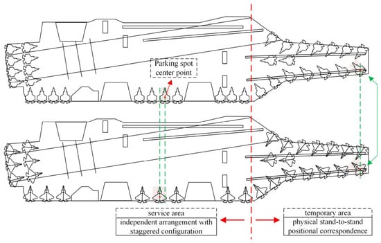
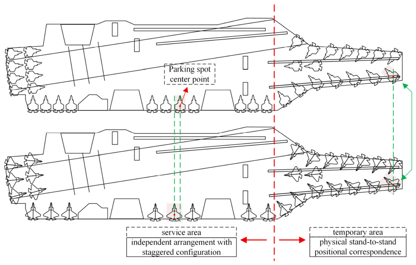
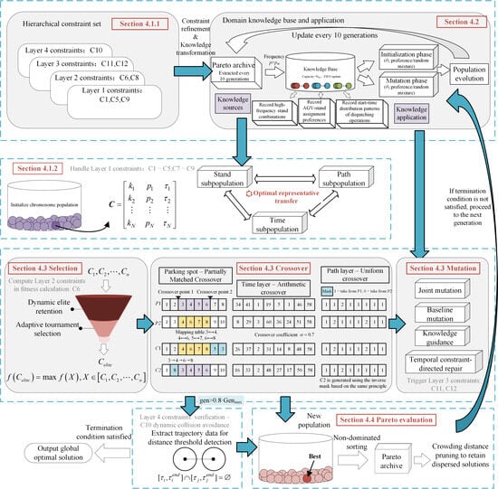
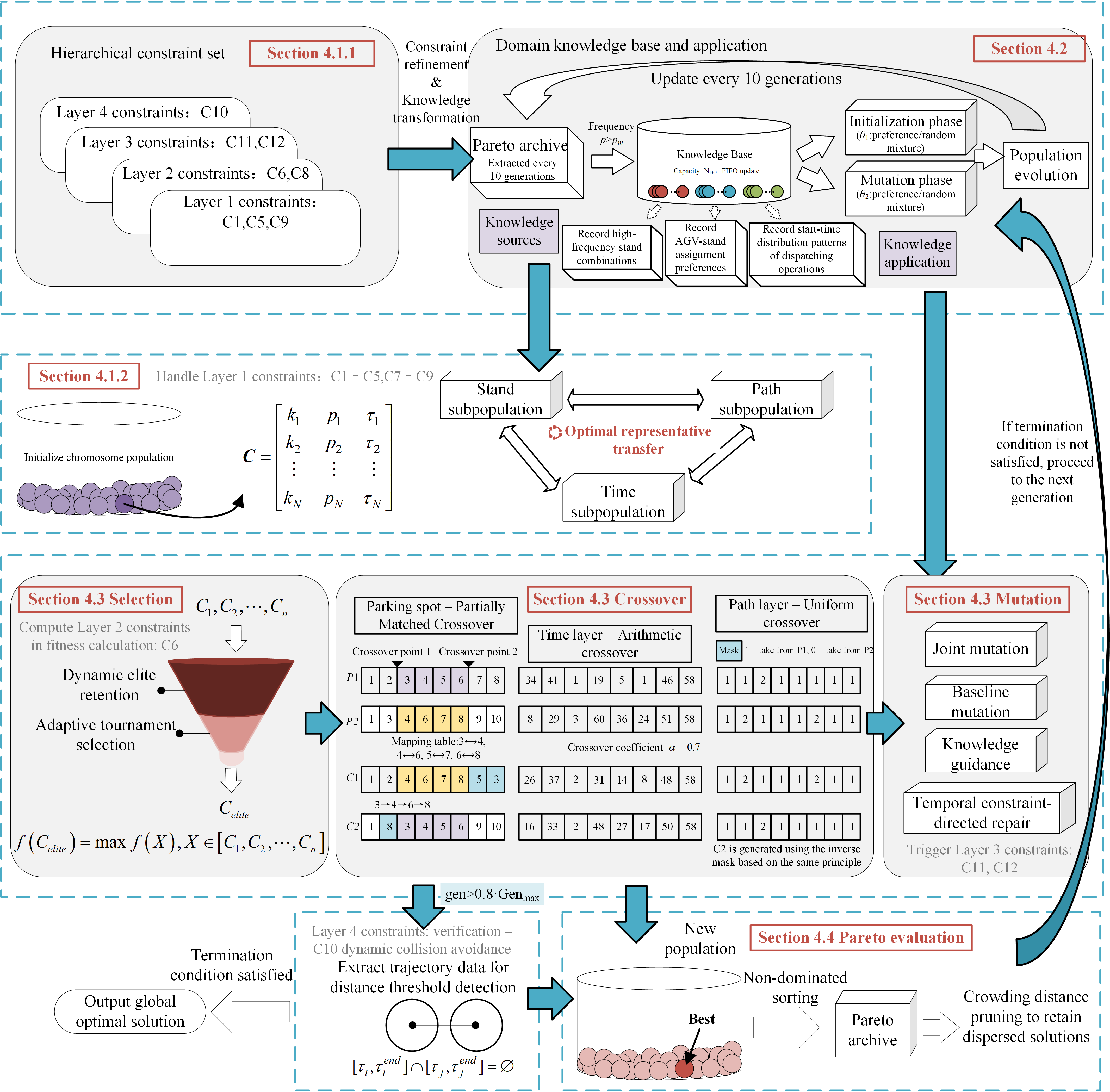
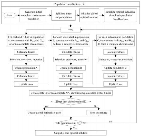
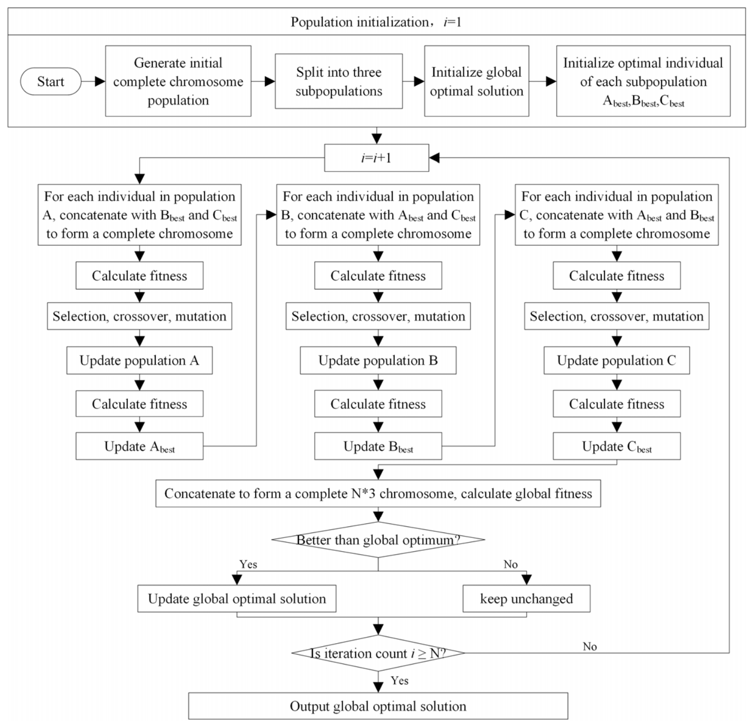
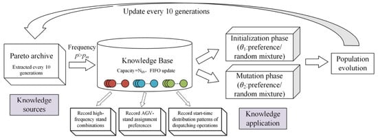
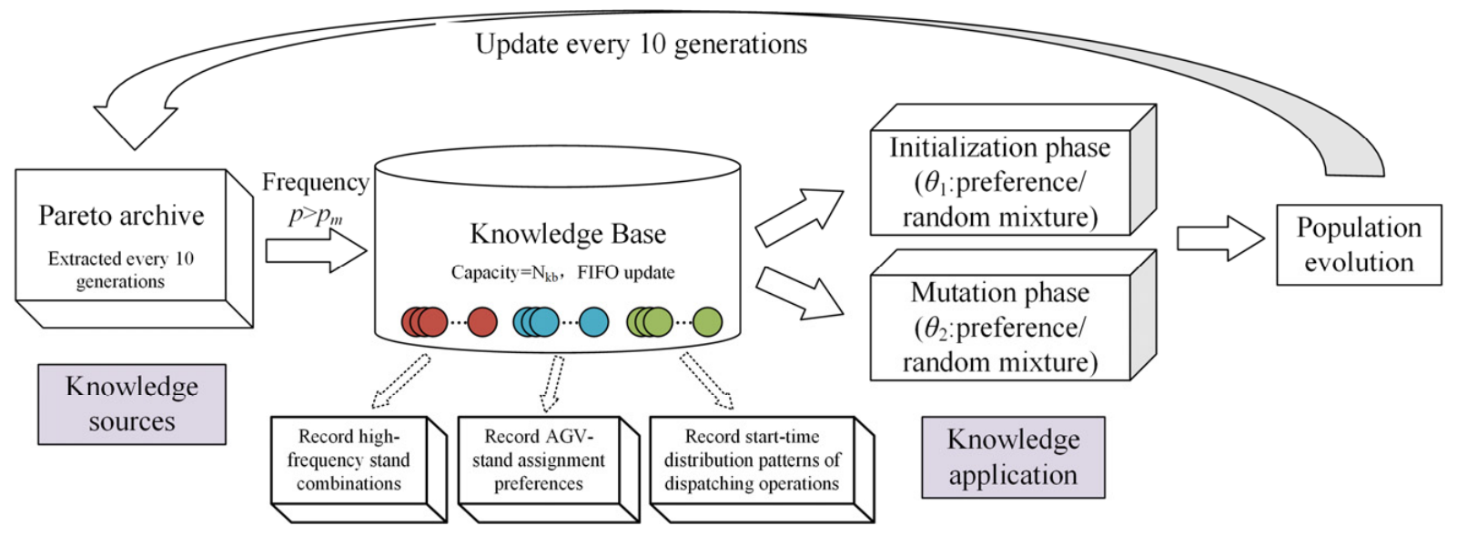
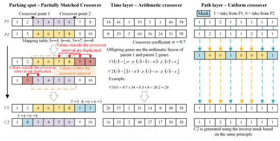
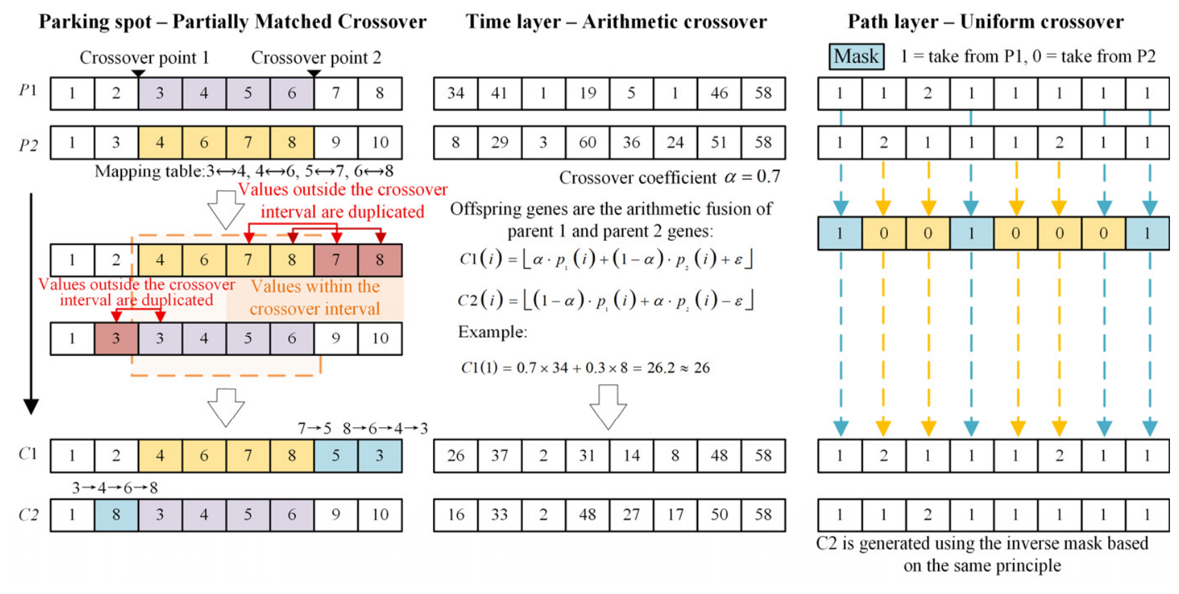
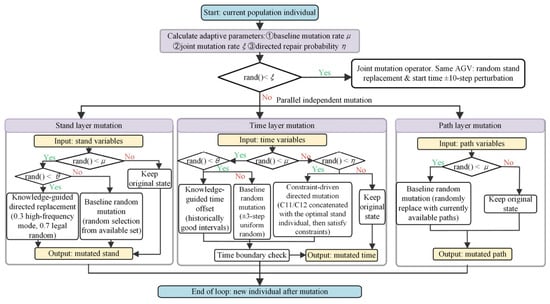
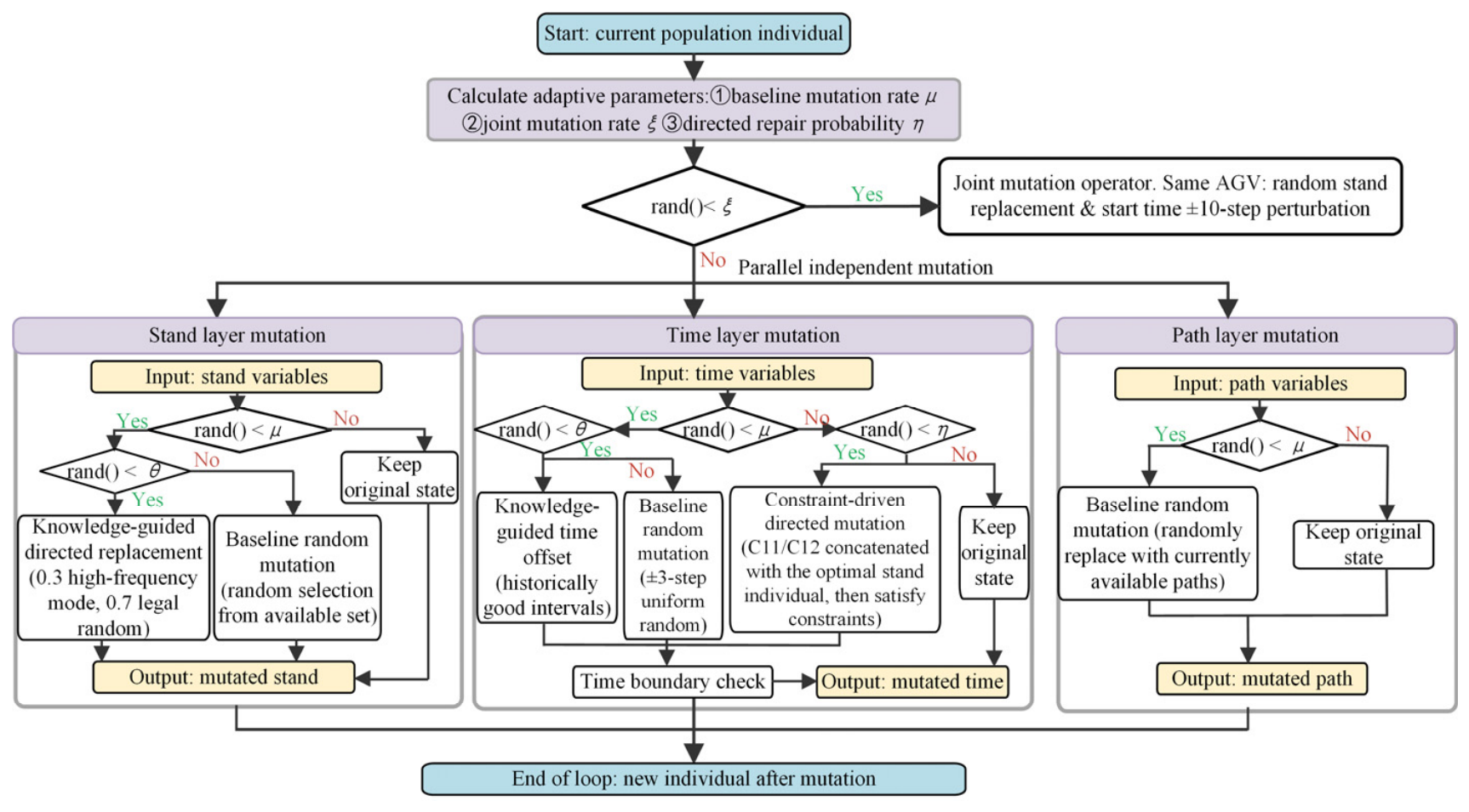
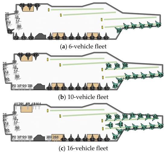
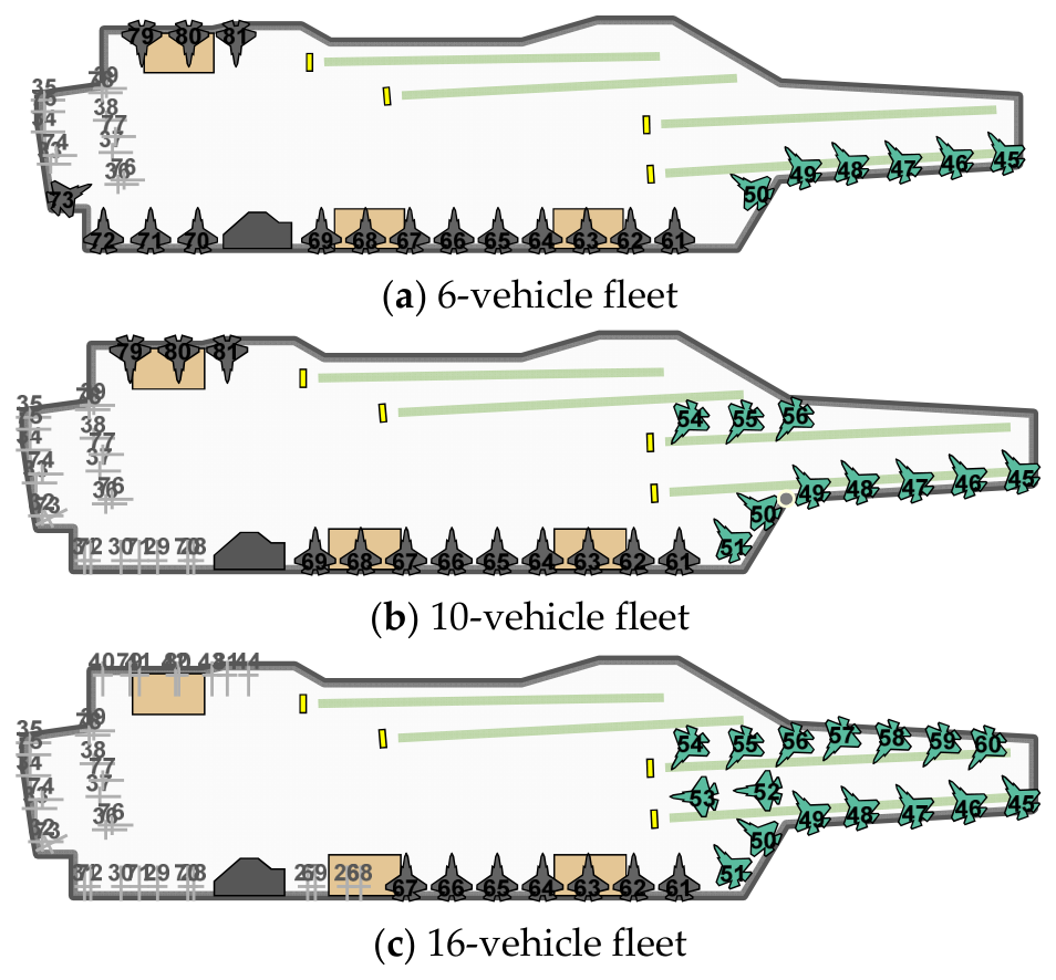


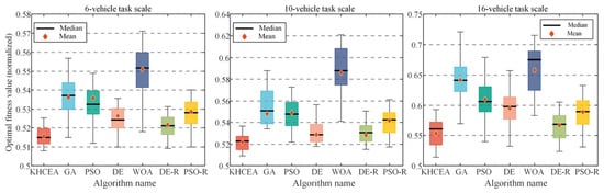
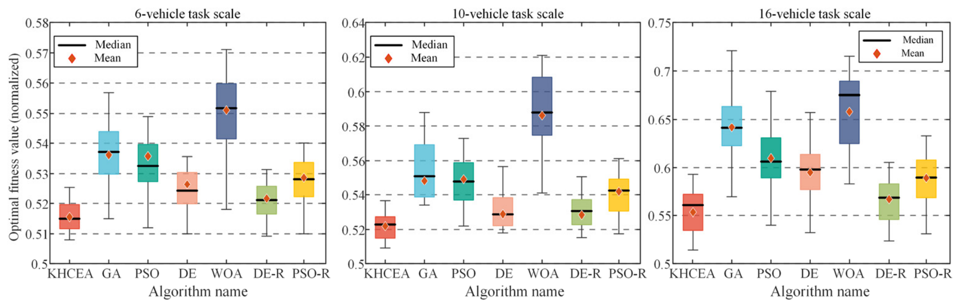
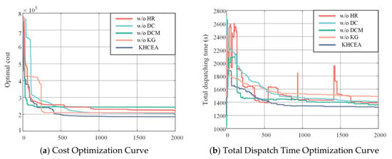
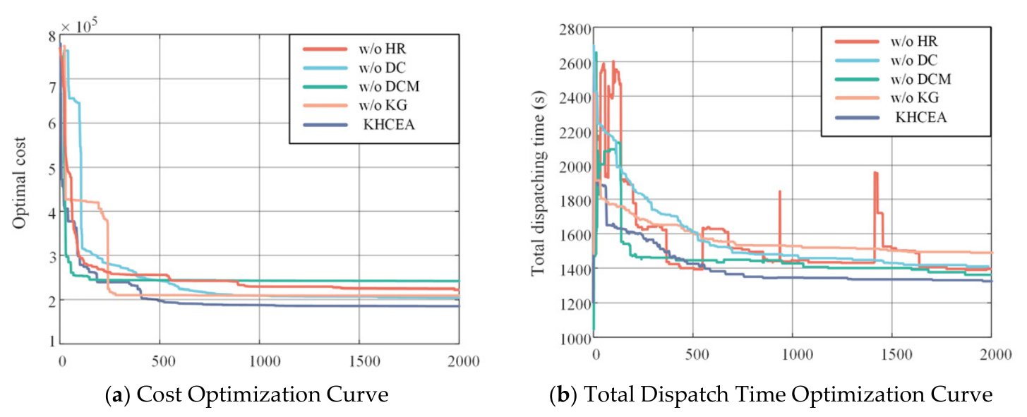
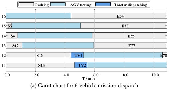
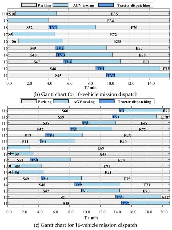
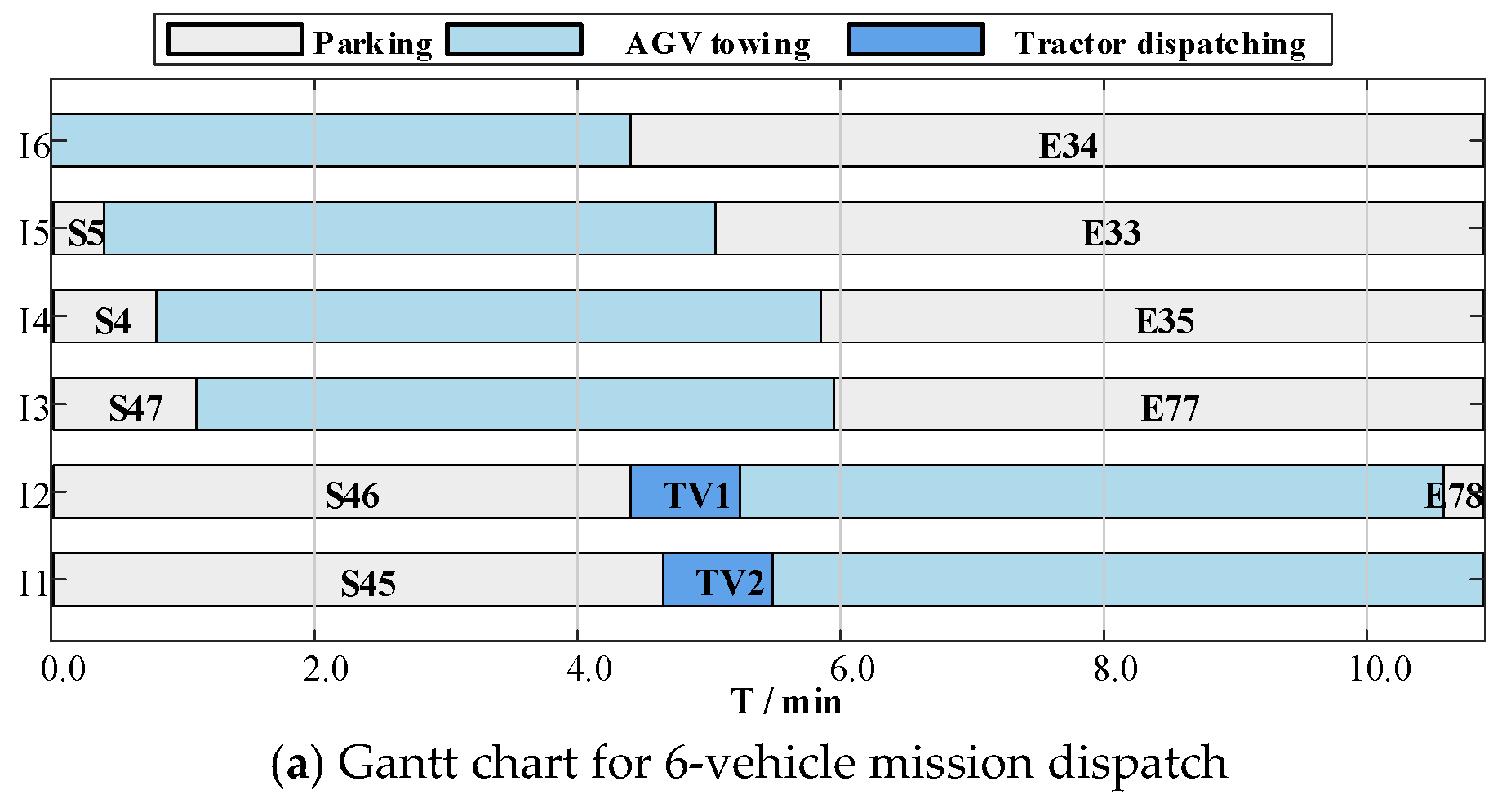
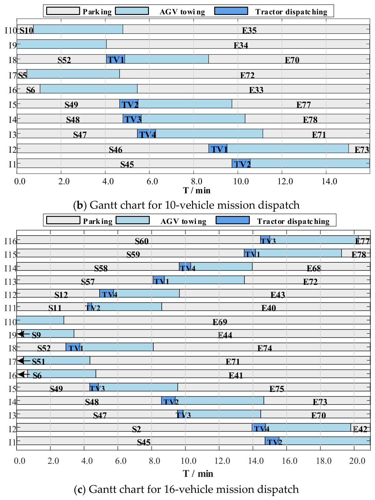
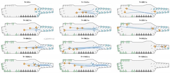
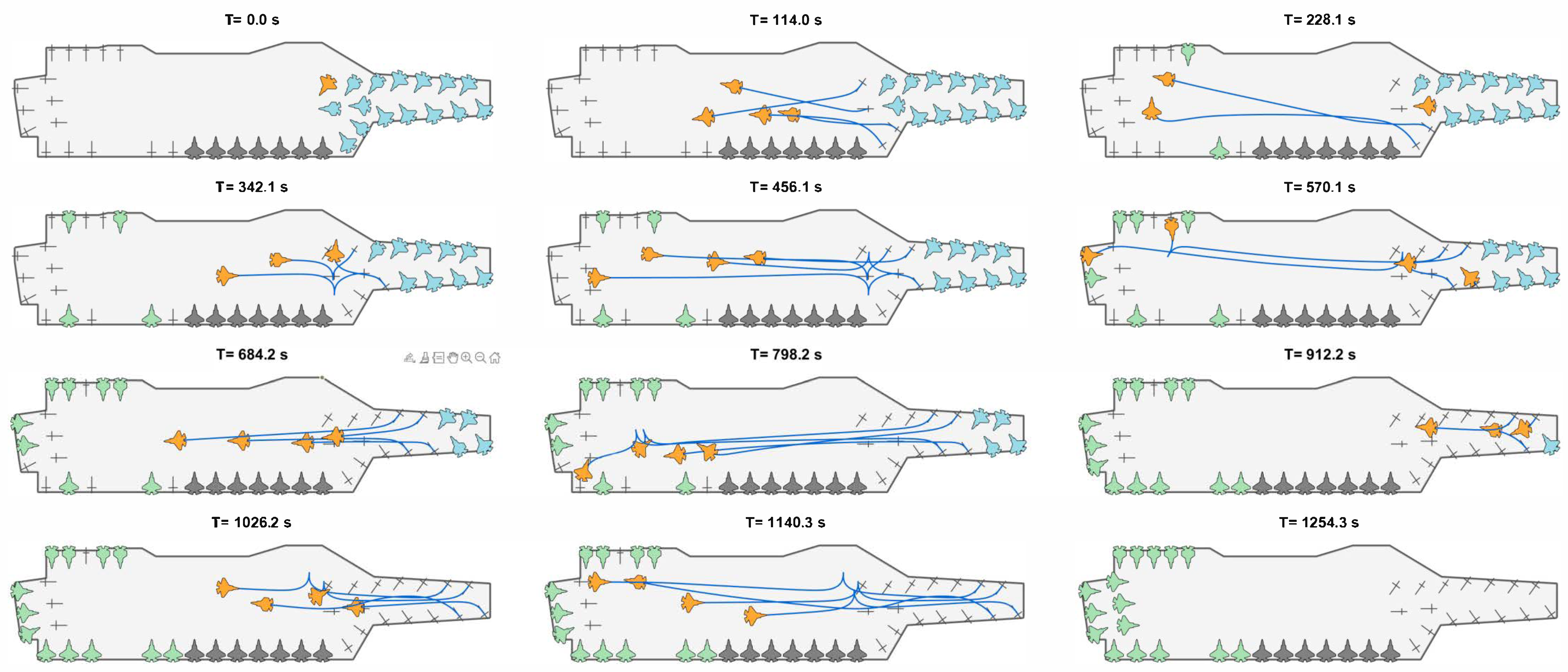

Disclaimer/Publisher’s Note: The statements, opinions and data contained in all publications are solely those of the individual author(s) and contributor(s) and not of MDPI and/or the editor(s). MDPI and/or the editor(s) disclaim responsibility for any injury to people or property resulting from any ideas, methods, instructions or products referred to in the content. |
© 2026 by the authors. Licensee MDPI, Basel, Switzerland. This article is an open access article distributed under the terms and conditions of the Creative Commons Attribution (CC BY) license.