Effects of PCI Trigger Thresholds on Construction Carbon Emissions and Pavement Performance in Hot In-Place Recycling of Xinjiang Expressways

Abstract

This deterministic scenario study examines how PCI trigger thresholds influence treatment timing, pavement condition, and cumulative construction-stage greenhouse-gas emissions for 4 cm hot in-place recycling within a boundary covering material production, transport, mixing, and on-site construction. Using project-derived deterioration parameters for nine Xinjiang expressway sections, annual simulations compared 4 cm hot in-place recycling rules over a 15-year horizon. Thirty-three rules combined pavement condition index (PCI) thresholds of 70–80 with assumed treatment gains of 5, 10 or 15 points. Each rule was evaluated under baseline parameters and twelve one-at-a-time perturbations of $\pm 5\%$ and $\pm 10\%$. Feasibility required every section to maintain a pre-treatment PCI of at least 70 throughout the horizon. Thirteen rules were feasible at baseline, and eleven remained feasible in all 13 parameter scenarios. The selected thresholds were 76 at a 10-point gain and 75 at a 15-point gain, with baseline mean cumulative construction emissions of 11.8677 and 8.4770 $\mathrm{kg}{\mathrm{CO}}_2\mathrm{e}{\mathrm{m}}^{-2}$, respectively. At a 15-point gain, threshold 74 passed the $\pm 10\%$ endpoint checks but failed when $\alpha$ decreased by 5%. Raising the PCI floor to 71 changed the selected thresholds to 77 and 76 for the two gain scenarios. The methodological contribution is an exhaustive integer-threshold scan coupled with section-wise feasibility screening across both endpoint and intermediate deterministic perturbations. The resulting thresholds are case-specific scenario outcomes, not probabilistic reliability estimates or whole-life carbon savings, and remain conditional on the adopted deterioration parameters, treatment gains, system boundary, and tested scenarios.

1. Introduction

1.1. Current Research

Carbon emissions from expressway maintenance cannot be assessed from a single intervention alone. The timing and frequency of the same treatment over a planning horizon alter its cumulative emissions. Road life-cycle studies have incorporated maintenance activities into emission inventories [1]. A review of life-cycle assessments for road and rail infrastructure found that the treatment of analysis periods and maintenance frequency affects the results [2]. Evaluations of pavement maintenance effectiveness increasingly consider both environmental burdens and retained performance [3].

Emissions from individual recycling interventions, including hot in-place recycling, have been quantified in previous studies. Energy use and carbon emissions have been compared across recycling methods [4], and life-cycle assessment results have informed pavement management systems [5]. Research in Xinjiang has also compared the dynamic life-cycle emissions of several asphalt pavement maintenance techniques [6]. Together, these studies indicate that both the emissions of an intervention and its timing warrant evaluation. The emission factor used here for treatment G comes from the source material described in Section 3.1; the cited studies provide context rather than the primary source for that parameter. Once the treatment is fixed, managers must still decide when to apply it and how long to wait before repeating it. This study therefore focuses on trigger-threshold selection within the eligible condition range for G and examines how the resulting treatment schedule changes cumulative emissions and pavement condition.

Several methods have been used to determine maintenance schedules. A multi-objective differential evolution algorithm has been applied to network-level planning [7], while life-cycle assessment and life-cycle cost analysis have informed preventive maintenance timing [8]. Project-level research has arranged repeated interventions into continuous schedules over a planning horizon [9], and reinforcement learning has been used for large-scale maintenance planning on multilane expressways [10]. Although carbon emissions and maintenance timing have been studied jointly, a narrower question remains: how do different scheduling rules for the same treatment compare.

Network-level models have also incorporated annual budgets [11] and their allocation [12]. Bayesian decision support can assist pavement management [13], and multi-agent reinforcement learning can address interdependent road sections [14]. A recent network model considers both low-carbon objectives and recycled material use [15]. These approaches accommodate many decision variables, but the contribution of any one factor to the final outcome can be difficult to isolate. Because the present study has one treatment and a limited set of section parameters, an interpretable account of why a rule works is more useful here than a more elaborate search algorithm.

Maintenance rules must also account for pavement performance. Fuzzy logic has been used to predict PCI [16], Bayesian dynamic models can provide probabilistic condition forecasts [17], and transition matrices describe deterioration at different time steps [18]. Climate-change research indicates that external conditions may alter pavement distress progression [19], while probabilistic long-term performance prediction continues to advance [20]. An urban-network study has included greenhouse gas emissions directly in maintenance scheduling objectives [21]. These developments suggest that a low-emission rule should also satisfy a pavement-condition constraint; a recommendation derived from one baseline parameter set may cease to be feasible when those parameters change.

1.2. Research Gap

Existing emission studies can supply the emissions of one maintenance event, but that value does not directly describe cumulative emissions over 15 years. Changing maintenance schedules and incomplete data complicate the accounting of maintenance-stage carbon emissions [22]. System boundaries also differ across asphalt pavement life-cycle assessments [23], and variation in input data can affect the results [24]. The source material used here gives construction emissions per unit area for G, but not the cumulative emissions associated with alternative annual schedules. Linking each annual treatment decision to this factor is necessary to quantify the effect of the scheduling rule.

Mixed-integer linear programming has been used for pavement maintenance decisions in high-altitude regions [25]. Other studies combine deep learning predictions with sustainability assessment in urban pavement management [26] or use multi-objective methods to compare maintenance and rehabilitation options [27]. These approaches broaden the environmental, performance, and decision objectives considered. For the hot in-place recycling treatment G examined here, however, it remains necessary to establish how PCI trigger thresholds affect treatment years, event counts, and cumulative construction emissions under the same eligibility conditions, and whether a rule feasible at baseline maintains the condition floor when deterioration parameters change. For this G-only case, the question is therefore narrower than selecting among maintenance technologies: under the same treatment and per-event emission factor, how does changing the PCI trigger threshold alter treatment years, event counts, cumulative construction emissions, and the lowest condition reached? Answering this question also requires testing whether a rule that passes under fitted deterioration parameters continues to pass when those parameters are perturbed.

The recommended rule also depends on the PCI gain that G can actually deliver and on the accuracy of baseline deterioration parameters. Post-maintenance performance forecasts have informed maintenance plans [28], and pavement monitoring and machine learning provide inputs to those forecasts [29]. Multi-attribute methods can be used to evaluate candidate treatments [30]. The available source gives a PCI gain range of 5–15 points for G. Treating a 15-point gain as a freely selectable outcome, then choosing the lowest-emission rule under unperturbed parameters, would yield an optimistic recommendation. Gains must instead be considered as separate scenarios, and selected rules must meet the PCI floor under prespecified parameter perturbations.

1.3. Study Scope and Contributions

This study uses PCI deterioration parameters from nine representative expressway sections in Xinjiang and the parameters of a 4 cm hot in-place recycling treatment (G) to conduct a 15-year scenario analysis of maintenance scheduling. The methodological contribution is the combination of an exhaustive integer-threshold scan with a section-wise feasibility screen under endpoint and intermediate deterministic parameter perturbations, whereas the resulting threshold values are case-specific numerical outcomes for the nine selected sections. Its contributions are as follows:

(1) Quantifying how integer PCI trigger thresholds alter treatment timing, intervention counts and cumulative construction emissions under a common treatment specification;

(2) Comparing thresholds separately for each assumed PCI gain while enforcing a minimum pre-treatment PCI for every section and year;

(3) Testing endpoint and intermediate deterioration-parameter perturbations to identify missed feasibility failures, and examining how the required condition margin changes the selected rule.

The section-level deterioration parameters, the G emission and cost inputs, and the estimated treatment-gain range were adopted from the project materials. The original analysis in this article is the complete 33-rule PCI-trigger scan, the 13-scenario section-wise feasibility screen, and the comparison of how the required PCI floor changes the feasible rule set. PCI 70 is a study-specific condition floor, and the selected numerical thresholds are conditional case-study results.

2. Materials and Methods

2.1. Study Framework

This study uses inputs from an internal project report on carbon-emission accounting and mitigation potential in Xinjiang expressway maintenance. These inputs include pavement deterioration parameters for nine expressway sections and an emission benchmark for hot in-place recycling. Section 2 describes the simulation and evaluation methods, while Section 3 presents the data sources and case-study inputs in detail. Expressway maintenance has an inherent time dimension. An intervention incurs carbon emissions and costs when implemented, while its subsequent effects appear in service life and pavement performance. A comparison confined to emissions from a single construction event can miss differences over the service period. Conversely, scheduling solely by pavement condition does not capture the emissions associated with more frequent intervention. We examine 4 cm hot in-place recycling as the sole treatment and assess how the PCI trigger threshold and assumed gain affect annual treatment timing. Section-specific PCI deterioration parameters describe condition trajectories; the unit emission factor for G is used to calculate cumulative emissions; and feasibility requires the lowest pre-treatment PCI across all sections and years to remain at or above 70. The aim is to identify scheduling rules that satisfy the pavement-condition constraint while limiting emissions for a fixed treatment, rather than to compare different maintenance technologies.

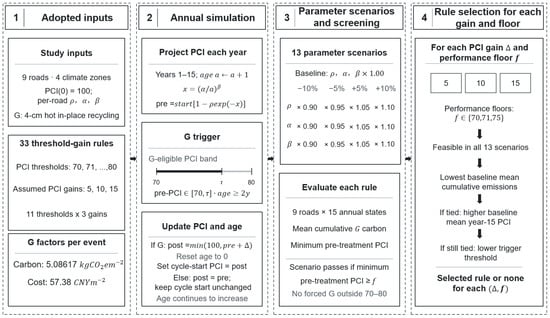
PCI was updated annually for each section over a 15-year horizon. At the start of each year, the virtual maintenance age was increased before pre-treatment PCI was calculated. G was applied only when pre-treatment PCI was within 70–80 and no higher than the rule’s trigger threshold, and at least two years had elapsed since the previous intervention. Following treatment, PCI was increased by the gain assumed for that scenario and the virtual maintenance age was reset to zero. Without treatment, the PCI at the start of the existing maintenance cycle remained unchanged and virtual age continued to increase. For each rule, we recorded treatment counts for the nine sections, their equally weighted mean cumulative construction emissions, the minimum pre-treatment PCI across sections and years, and mean PCI in year 15. Direct construction cost was reported only as a secondary outcome. The overall workflow of this study, including the adopted project inputs, annual PCI simulation, deterministic parameter-perturbation screening, and rule selection under different PCI gains and performance floors, is illustrated in Figure 1.

Figure 1. Study workflow.

Section 4 presents the baseline screening, comparison of feasible rules, and sensitivity analysis.

2.2. Unit Emission Factor for Treatment G

The value of $5086.17 \mathrm{kg}{\mathrm{CO}}_2\mathrm{e}/1000 {\mathrm{m}}^2$ was adopted as the inventory-based benchmark for the 4 cm G treatment from the project materials. The project describes its treatment-specific emission benchmarks as arithmetic means of results from eight case-study sections; these emission-accounting cases are distinct from the nine sections used in the PCI scheduling analysis. It is not a direct exhaust measurement from the nine sections used in the scheduling simulation. The estimate combines material quantities, transport and equipment activity, and energy-use coefficients with emission factors used in the project accounting. Its boundary covers material production, material transport, mixing, and on-site construction. Fuel-related emissions from transport and construction are included in the inventory, but the available summary does not separately quantify direct combustion and upstream fuel-supply emissions. The adopted direct construction cost is 57,384.6 $\mathrm{CNY}/1000 {\mathrm{m}}^2$.

The available materials do not establish a separate observation year or an empirical uncertainty distribution for this 4 cm emission benchmark. We therefore treat it as a fixed input and examine a common ±10% change only as an illustrative deterministic scaling test, not as a measured uncertainty interval:

$$\begin{array}{cc}\hfill e_G& =5.08617 \mathrm{kg}{\mathrm{CO}}_2\mathrm{e}{\mathrm{m}}^{-2}\hfill \\ \hfill k_G& =57.3846 \mathrm{CNY}{\mathrm{m}}^{-2}\hfill \end{array}$$

For section i under rule p, cumulative carbon emissions and direct construction cost were calculated as:

$$\begin{array}{c}\hfill C_{i,p}=e_G{\displaystyle \sum _{t=1}^{15}}{z}_{i,t,p}\\ \hfill K_{i,p}=k_G{\displaystyle \sum _{t=1}^{15}}{z}_{i,t,p}\end{array}$$

Here, $C_{i,p}$ and $K_{i,p}$ denote cumulative emissions and cost for section i under rule p; $z_{i,t,p}$ indicates whether treatment G was applied to that section in year t. It equals 1 when G was applied $z_{i,t,p}=1$ and 0 otherwise $z_{i,t,p}=0$. No temporal discounting was applied. Cumulative cost was reported as an undiscounted direct construction cost and did not enter rule selection or ranking.

2.3. Pavement-Condition Evolution and Scheduling of G

2.3.1. Deterioration Model

PCI was the sole pavement-state variable used to schedule G. It determined annual treatment eligibility, compliance with the minimum service-level constraint, and end-of-horizon condition. In the underlying decision table, G is listed as an option at PCI 70–80 in both RQI bands, 0–80 and 80–100. Thus, removing the RQI subdivision does not change whether G is listed within the PCI interval examined here. The source table also lists G in some states above PCI 80 and below PCI 70, which our narrower rule excludes. Although RQI deterioration parameters are reported, no post-G RQI recovery parameter is available. We therefore assess PCI feasibility only and cannot claim that the selected rules satisfy a combined PCI–RQI requirement.

PCI as a function of virtual age was represented by:

$$\begin{array}{c}\hfill {\mathrm{PCI}}_{i,t}^{\mathrm{pre}}=\left\{\begin{array}{cc}{\mathrm{PCI}}_{i,c},\hfill & a_{i,t}^{-}=0,\hfill \\ {\mathrm{PCI}}_{i,c}\left[1-{\rho }_i\exp \left(-{\left({\displaystyle \frac{{\alpha }_i}{a_{i,t}^{-}}}\right)}^{{\beta }_i}\right)\right],\hfill & a_{i,t}^{-}>0.\hfill \end{array}\right.\end{array}$$

Here, ${\mathrm{PCI}}_{i,c}$ is the PCI at the start of the current virtual maintenance cycle, and $a_{i,t}^{-}$ is the pre-decision virtual age in years. Parameter ${\rho }_i$ is dimensionless and controls the asymptotic fractional PCI loss; ${\alpha }_i$ has units of years and controls the deterioration time scale; and ${\beta }_i$ is dimensionless and controls the curve shape. These parameters describe fitted section-level trajectories and are not independently measured physical properties. Because the original pavement-condition observations and calibration diagnostics were unavailable, the predictive accuracy of these fitted trajectories could not be independently assessed. After G, the simulated post-treatment PCI became the starting condition of a new virtual maintenance cycle, and virtual age was reset to zero. The same section-specific deterioration parameters were reused in subsequent cycles. This repeated-treatment assumption was not calibrated against observed successive G interventions on the nine sections. Reusing the same deterioration parameters and gain allows threshold rules to be compared under a common treatment-response convention. Because event-specific PCI recovery and post-treatment deterioration records are unavailable, the simulated schedules are conditional comparisons rather than validated forecasts of successive field interventions.

2.3.2. Trigger Rule and State Update for G

Treatment G denotes hot in-place recycling. Its timing depends jointly on current PCI and virtual age since the most recent G event. Let $z_{i,t,p}$ be the annual treatment decision. When $z_{i,t,p}=1$, section i receives G in year t; when $z_{i,t,p}=0$, it remains untreated and advances to the next year.

Before year 1, cycle-start PCI was set to 100 and post-decision virtual age was set to zero for every section. In each year, we first increased virtual age by one and calculated pre-treatment PCI from the current cycle-start PCI. We recorded a violation if this pre-treatment value was below the specified condition floor. We then applied G only if pre-treatment PCI was within 70–80, was no higher than the rule’s trigger threshold, and virtual age was at least two years. Following treatment, PCI increased by the assumed gain, subject to a cap of 100; the resulting PCI became the start of a new virtual cycle and post-decision age became zero. Without treatment, the existing cycle-start PCI was retained and post-decision age equaled that year’s pre-decision age. Before the following year’s decision, age increased by one again. Consequently, age is one in the year immediately after a treatment and two in the second year. A treatment cannot erase a condition-floor violation recorded earlier in the same year:

$$\begin{array}{c}\hfill z_{i,t,p}=\left\{\begin{array}{cc}1,\hfill & 70\le {\mathrm{PCI}}_{i,t}^{\mathrm{pre}}\le \min ({\tau }_p,80)\mathrm{and}{a}_{i,t}^{-}\ge 2,\hfill \\ 0,\hfill & \mathrm{otherwise}.\hfill \end{array}\right.\end{array}$$

Here, ${\mathrm{PCI}}_{i,t}^{\mathrm{pre}}$ is the pre-treatment PCI of section i in year t, ${\tau }_p$ is the PCI trigger threshold for rule p, and $a_{i,t}^{-}$ is virtual age before the annual decision. A year in which pre-treatment PCI falls below 70 still counts as a violation of the performance constraint, but G is no longer applied because the section has left its simulated eligibility range. A later intervention cannot erase that violation. The upper bound of design service life does not trigger mandatory treatment.

When G was applied, PCI was first updated by the assumed gain and virtual age was then reset to zero. Otherwise, pre-treatment PCI became the post-decision state for the next year. Eleven integer PCI thresholds from 70 to 80 and three assumed PCI gains formed 33 rule–effect scenarios. Gain represented a possible performance level of the same treatment, not a decision variable that could be selected independently in each year:

$$\begin{array}{c}\hfill {\mathrm{PCI}}_{i,t}^{\mathrm{post}}=\left\{\begin{array}{cc}\min \{100,{\mathrm{PCI}}_{i,t}^{\mathrm{pre}}+\Delta \},\hfill & z_{i,t,p}=1,\hfill \\ {\mathrm{PCI}}_{i,t}^{\mathrm{pre}},\hfill & z_{i,t,p}=0.\hfill \end{array}\right.\end{array}$$

Here, ${\mathrm{PCI}}_{i,t}^{\mathrm{pre}}$ and ${\mathrm{PCI}}_{i,t}^{\mathrm{post}}$ are pre- and post-treatment PCI in year t; $z_{i,t,p}=1$ and $z_{i,t,p}=0$ indicate that G was and was not applied, respectively; and $\Delta$ is the PCI gain assumed for that scenario. Post-treatment PCI was capped at 100.

Virtual age was updated with the treatment decision:

$$\begin{array}{c}\hfill a_{i,t}^{+}=\left\{\begin{array}{cc}0,\hfill & z_{i,t,p}=1,\hfill \\ a_{i,t}^{-},\hfill & z_{i,t,p}=0,\hfill \end{array}\right.a_{i,t+1}^{-}=a_{i,t}^{+}+1\end{array}$$

Here, $a_{i,t}^{+}$ is virtual age after the year’s decision; virtual age before the following year’s decision is $a_{i,t+1}^{-}=a_{i,t}^{+}+1$. In a treatment year, post-decision age is zero and reaches one before the next year’s decision. Post-treatment trajectories were used for annual scheduling only within the stated scenarios; the assumed gain was not extrapolated as an indefinitely persistent observed treatment effect.

2.4. Rule Evaluation and Deterministic Sensitivity Analysis

With a fixed, undiscounted emission factor per G event, cumulative construction emissions over the planning horizon depend only on the number of interventions. Each G event incurs the same event-level emissions and cost, allowing annual decisions to be converted directly to cumulative totals using the factors defined in Section 2.2.

For section i under rule p, the minimum pre-decision PCI during the planning horizon and PCI at the end of year 15 were defined as:

$$\begin{array}{c}\hfill {\mathrm{PCI}}_{i,p}^{\min }=\underset{t=1,\dots ,15}{\min }{\mathrm{PCI}}_{i,t}^{\mathrm{pre}}\\ \hfill {\mathrm{PCI}}_{i,p}^{15}={\mathrm{PCI}}_{i,15}^{\mathrm{post}}\end{array}$$

Let ${\mathrm{PCI}}_{i,t,p,s}^{\mathrm{pre}}$ and ${\mathrm{PCI}}_{i,t,p,s}^{\mathrm{post}}$ denote PCI immediately before and after the treatment decision in year t, under rule p and parameter scenario s. The minimum pre-treatment PCI is $M_{i,p,s}={\min }_{t=1,\dots ,15}{\mathrm{PCI}}_{i,t,p,s}^{\mathrm{pre}}$. The end-of-horizon PCI is $E_{i,p,s}={\mathrm{PCI}}_{i,15,p,s}^{\mathrm{post}}$, namely the post-decision PCI at the end of year 15.

Cumulative emissions, cumulative direct cost, and year-15 PCI were summarized for each rule as unweighted means across the nine representative sections:

$$\begin{array}{c}\hfill C_p={\displaystyle \frac{1}{9}}{\displaystyle \sum _{i=1}^9}{C}_{i,p}\\ \hfill K_p={\displaystyle \frac{1}{9}}{\displaystyle \sum _{i=1}^9}{K}_{i,p}\\ \hfill {\overline{\mathrm{PCI}}}_{15,p}={\displaystyle \frac{1}{9}}{\displaystyle \sum _{i=1}^9}{\mathrm{PCI}}_{i,p}^{15}\end{array}$$

Here, ${\mathrm{PCI}}_{i,p}^{\min }$ is the lowest pre-treatment PCI of section i under rule p over the 15-year horizon, and ${\mathrm{PCI}}_{i,p}^{15}$ is its post-decision PCI at the end of year 15. Because section length, traffic volume, and lane count were not used as weights, these values describe an equally weighted comparison of nine sections, not a Xinjiang-wide network average. As all rules share the same emission factor per G event, mean cumulative emissions equal the total number of treatments across the nine sections multiplied by that factor and divided by nine. If $N_p$ is the total number of G events across the nine sections under rule p, the reported equally weighted mean is $C_p=N_p{e}_G/9$. Thus, 21 events give $21\times 5.08617/9=11.8677 \mathrm{kg}{\mathrm{CO}}_2\mathrm{e}{\mathrm{m}}^{-2}$, and 15 events give $15\times 5.08617/9=8.4770 \mathrm{kg}{\mathrm{CO}}_2\mathrm{e}{\mathrm{m}}^{-2}$. These are mean cumulative emissions per square meter for one of the selected sections, not the total emissions of the nine-section road network.Within a given gain scenario, ranking rules by baseline cumulative emissions is therefore equivalent to ranking them by the aggregate treatment count. A common positive change in the per-event emission factor scales all cumulative emissions proportionally and leaves the ranking unchanged. This invariance does not apply when per-event emissions differ among sections, treatment years or construction conditions. Minimum pre-treatment PCI and mean year-15 PCI describe the condition associated with those emission differences.

A rule was screened against the requirement that no section fall below PCI 70 before treatment in any year:

$$\begin{array}{c}\hfill \underset{i,t}{\min }{\mathrm{PCI}}_{i,t}^{\mathrm{pre}}\ge 70\end{array}$$

The primary performance floor was PCI 70. It was chosen to test G-only rules against the lower bound of the modeled G eligibility interval and is a scenario assumption, not a universal road-management standard. The source study used PCI 75 in a different, multi-treatment optimization. To assess the effect of this choice, we repeated the present G-only screening at PCI floors of 71 and 75. Each floor applies to every section and year before the annual treatment decision; treatment in the same year cannot erase a pre-treatment violation. Within each assumed gain scenario, a rule was selected only after it passed the specified floor in all 13 deterioration-parameter scenarios. Feasible rules were ranked by baseline mean cumulative construction emissions, with higher baseline mean year-15 PCI and then the lower threshold used to break ties.

Each of the 33 rules was evaluated under 13 prescribed deterioration-parameter scenarios: the fitted baseline and twelve one-at-a-time perturbations. For each of $\rho$, $\alpha$, and $\beta$ in turn, the parameter values for all nine sections were multiplied by 0.90, 0.95, 1.05, or 1.10 while the other two parameters remained unchanged. We recorded treatment counts, mean cumulative construction emissions, and the lowest pre-treatment PCI for each rule and scenario. For an assumed gain $\Delta$ and a PCI floor $f\in \{70,71,75\}$, a rule was feasible only if the lowest pre-treatment PCI across all nine sections and 15 years met f in every scenario. The ±5% cases were included because discrete annual decisions can fail between the tested ±10% endpoints. These prescribed changes are stress tests, not fitted confidence limits; they do not assess joint parameter changes, failure probabilities, or every value between the tested points.

For each gain, we simulated annual states for all nine sections under baseline parameters and the twelve one-factor perturbations. Feasibility in each parameter scenario was determined from the minimum pre-treatment PCI across all sections and years; a mean PCI across sections cannot replace that constraint. For each assumed PCI gain $\Delta$ and performance floor $f\in \{70,71,75\}$, a rule entered the feasible set only if the minimum pre-treatment PCI across all nine sections and 15 years met that floor in every one of the 13 parameter scenarios:

$${\mathcal{R}}_{\Delta ,f}=\left\{p\in {\mathcal{P}}_{\Delta }:\underset{i,t}{\min }{\mathrm{PCI}}_{i,t}^{\mathrm{pre}}(p,s)\ge f,\forall s\in \{1,\dots ,13\}\right\}.$$

(1)

Within each nonempty feasible set, we selected a rule by comparing the following quantities in order:

$$p^{*}(\Delta ,f)=\underset{p\in {\mathcal{R}}_{\Delta ,f}}{lex\; arg\; min}\left(C_{p,\Delta }^{\mathrm{baseline}},-{\overline{\mathrm{PCI}}}_{15,p,\Delta }^{\mathrm{baseline}},{\tau }_p\right).$$

(2)

Here, ${\mathcal{P}}_{\Delta }$ is the set of 11 integer-threshold rules evaluated at gain $\Delta$, and ${\mathcal{R}}_{\Delta ,f}$ is the subset that meets floor f in all 13 parameter scenarios. The selection is lexicographic: lower baseline mean cumulative emissions are preferred first; ties are broken by higher baseline mean year-15 PCI and then by the lower trigger threshold ${\tau }_p$. The analysis with $f=70$ is the primary analysis. The analyses with $f=71$ and $f=75$ repeat the same screening procedure as sensitivity analyses. If ${\mathcal{R}}_{\Delta ,f}$ is empty, no rule is selected for that gain and floor. Mean emissions across parameter scenarios are descriptive and are not used for ranking. The perturbations are not statistical confidence intervals, and simultaneous changes in multiple deterioration parameters were not assessed.

3. Data and Case-Study Design

3.1. Data Sources and Study Basis

This study uses case-study inputs from an internal project report entitled “Research on Carbon-Emission Accounting and Mitigation Potential in Xinjiang Expressway Maintenance”. The report is unpublished and not publicly accessible. Xinjiang Communications Investment Engineering Technology Development Co., Ltd. provided the input data. Nine sections supplied the fitted PCI parameters, an eight-section accounting exercise supplied the G emission benchmark, and records from 120 maintenance projects during 2021–2025 informed representative transport distances and direct costs. These datasets were used for different purposes and were not pooled as one sample. According to the project document, the section-specific deterioration parameters were fitted to historical pavement-condition records in MATLAB R2023b using a function defined with fittype. The PCI gain of 5–15 points was estimated from maintenance specifications and previous studies rather than measured following G treatment on the nine sections. The reported design service life of G was 2–4 years; the present scheduling rule uses two years as its minimum virtual maintenance age. Although Table 5.7 of the project document lists G among the options for several PCI–RQI states, this study restricted its scheduling scenario to pre-treatment PCI of 70–80 without an RQI subdivision. We adopted the nine fitted parameter sets without refitting the underlying monitoring data. The section-specific PCI deterioration parameters are presented in Table 1. The main parameters adopted for treatment G are summarized in Table 2. The equally weighted section results are case comparisons, rather than a network mean weighted by route length or traffic. The nine sections were selected to cover the four climatic zones represented in the project materials and to provide sections with comparatively complete condition records, clear maintenance histories, and identifiable deterioration trends. Selection was intentional rather than random.

Table 1. PCI deterioration parameters for representative expressway sections across four climatic zones.

Zone	Section	Road Section	Route	Chainage	$\mathit{\rho }$	$\mathit{\alpha }$	$\mathit{\beta }$
I	1	Sayram Lake–Horgos	G30	K4168 + 000–K4208 + 000	0.744	6.266	0.665
I	2	Wuxuete Township–Emin	G3015	K220 + 000–K250 + 000	0.575	5.388	0.623
II	3	Kuitun–Sayram Lake	G30	K3927 + 000–K3967 + 000	0.534	4.582	0.911
II	4	Karamay–Altay	G3014	K255 + 000–K295 + 000	0.516	4.875	0.832
III	5	Xingxingxia–Shanshan boundary	G30	K2825 + 000–K2855 + 000	0.604	8.235	0.865
III	6	Kuitun–Karamay	G3014	K30 + 000–K60 + 000	0.569	9.875	0.675
III	7	Jiashi General Farm–Kuguwan	G3012	K1210 + 000–K1240 + 000	0.719	9.406	0.697
IV	8	Shanshan boundary–Tuyugou	G30	K3225 + 000–K3265 + 000	0.677	13.342	0.779
IV	9	Xiaocaohu–Yushugou	G3012	K80 + 000–K120 + 000	0.643	15.176	0.664

Table 2. Main parameters for treatment G.

Parameter	Value
Assumed PCI gain per event	5, 10, or 15 points
Carbon emissions per G event ($\mathrm{kg}{\mathrm{CO}}_2\mathrm{e}{\mathrm{m}}^{-2}$)	5.08617
Direct cost per G event ($\mathrm{CNY}{\mathrm{m}}^{-2}$)	57.3846
Design service life	2–4 years

The scheduling analysis used project-derived parameters and did not include additional field monitoring or direct exhaust measurements. Table 3 reports the construction equipment, shift quantities and energy-use coefficients used in the adopted emission inventory. These coefficients were used for inventory-based accounting and do not represent instrument measurement accuracy. The available project materials do not provide the specifications or calibration records of the original PCI survey instruments; measurement uncertainty for the original surveys therefore could not be quantified.

Table 3. Equipment and energy-use coefficients for the 4 cm hot in-place recycling treatment per 1000 square metres.

Equipment Specification	Shifts per 1000 m2	Diesel Consumption (kg/Shift)	LPG Consumption (kg/Shift)
Liquid asphalt transport truck, capacity $\le 4000$ L	0.10	34.28	–
Asphalt paver, paving width $\le 4.5$ m	0.34	46.63	–
Double-drum vibratory roller, mass $\le 15$ t	0.48	80.80	–
Pneumatic-tyre roller, mass 20–25 t	0.64	50.40	–
Pavement heater	1.02	85.37	751.50
Heated milling machine	0.34	113.46	727.63
Heated remixing machine	0.34	128.72	882.16
Water truck, capacity $\le 10,000$ L	0.24	52.80	–

To make sections and rules comparable, the accounting unit was one square meter of pavement, the horizon was 15 years, and initial PCI was set to 100 for every section. Setting PCI to 100 gives the nine sections a common simulated starting condition; it does not assert that all nine sections had a measured PCI of 100 in the same calendar year. Treatment years and selected thresholds may differ under other starting conditions, which could not be tested without the corresponding observed initial states. The PCI 70 floor was a scenario-specific performance threshold applied to pre-treatment condition throughout the horizon, not a universal threshold for road management.

3.2. PCI Deterioration Parameters for Representative Sections

The source report used a three-parameter deterioration model to describe PCI as a function of service age. We adopted its section-specific PCI parameters to simulate performance without maintenance. Parameters $\rho$, $\alpha$, and $\beta$ for each section were inserted into the PCI equation in Section 2.3.1 to construct annual untreated and post-treatment trajectories from a common initial PCI.

The parameter sets in Table 1 differ across the nine sections and therefore generate different trajectories despite a common initial PCI and rule. These differences are used to parameterize heterogeneous scenarios; they do not isolate causal effects of climatic zone, traffic loading, or pavement material. The materials available for this analysis do not document the observation years, number of PCI surveys, or survey frequency for each of the nine sections. The available project materials provide the fitted deterioration parameters but not the observation-level PCI records, residuals or numerical fit diagnostics. Consequently, empirical prediction errors, goodness-of-fit statistics and parameter confidence intervals could not be estimated from the available data. The parameter perturbations examine the sensitivity of scheduling outcomes to prescribed input changes; they do not estimate measurement error or validate field predictive accuracy. The resulting thresholds should therefore be interpreted as conditional scenario results.

A separate recalculation of all 429 rule–scenario combinations reproduced treatment counts, minimum pre-treatment PCI and mean cumulative emissions to the reported precision. This check verifies numerical consistency and does not validate the deterioration model against field observations.

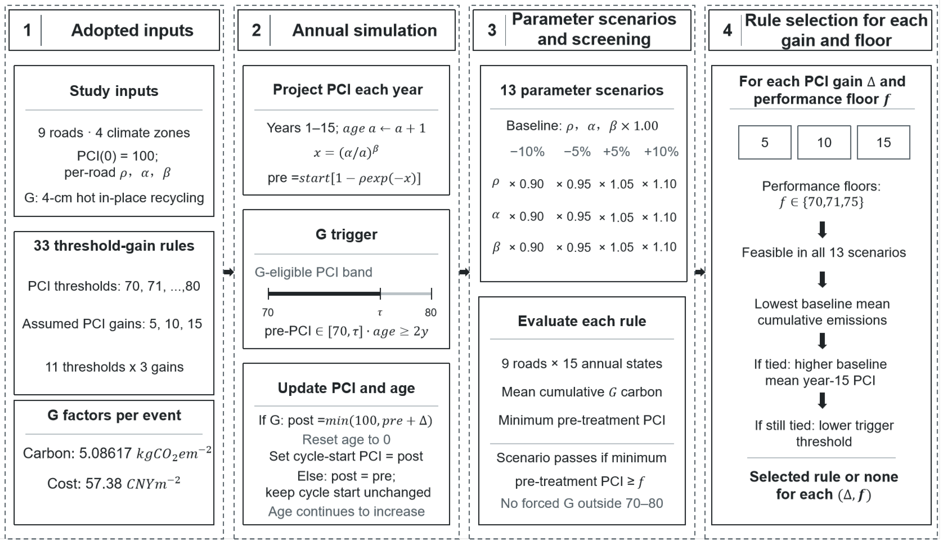
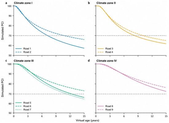
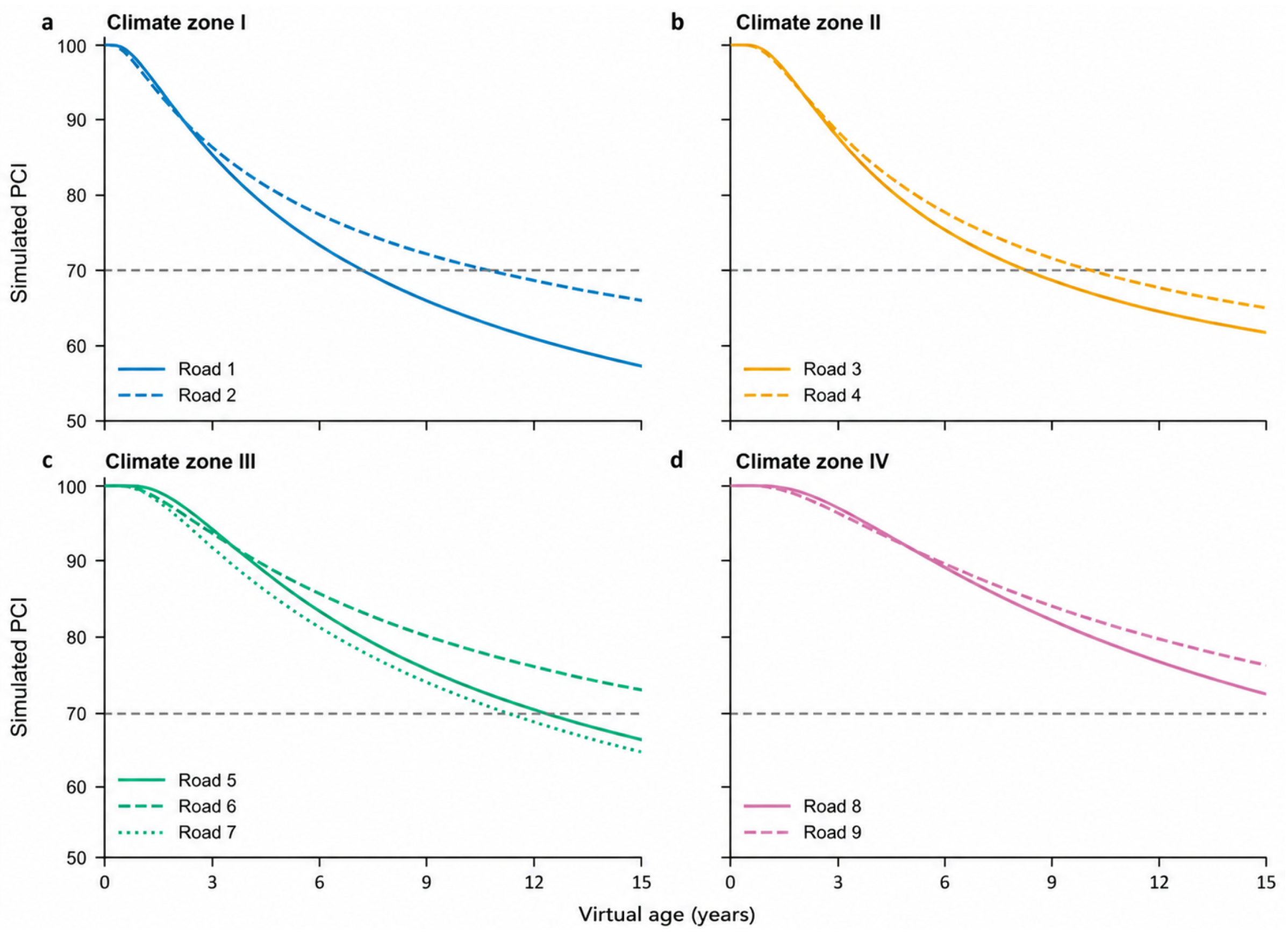
Figure 2 shows simulated PCI trajectories without maintenance using the parameters in Table 1. All sections start at PCI 100, and the dashed line marks the PCI 70 floor. The figure illustrates differences in the time taken to reach that floor; it is not a validated forecast of future PCI on those sections.

Figure 2. Simulated PCI trajectories for the nine representative sections without maintenance.

Without maintenance, section 1 first fell below PCI 70 in year 8, whereas section 9 remained at 76.5286 in year 15. Both began at the same PCI, so the difference in trajectories arose from the deterioration parameters in Table 1. A mean PCI across the nine sections could conceal an early floor violation on a faster-deteriorating section. Rule screening therefore used the lowest pre-treatment PCI across all sections and years.

3.3. Parameters for Hot In-Place Recycling

We selected hot in-place recycling, denoted treatment G, using the Xinjiang maintenance context and the emission estimates in the source report. This technique reuses existing asphalt pavement and can improve condition while reducing demand for new materials and transport. It therefore provides a case in which the effect of scheduling the same treatment on cumulative construction emissions can be examined.

In the project report Table 5.4 of the project materials lists an estimated PCI gain of 5–15 points for G. The project materials state that this planning estimate was developed with reference to the treatment-applicability guidance in JTG/T 5142-01—2021 [31] and prior research; the standard itself is not presented here as a measurement of PCI gain on the nine selected sections. In the present model, the gain is applied immediately to pre-treatment PCI in the treatment year and is capped at PCI 100. Gains of 5, 10, and 15 points define separate scenarios; each scenario applies its assumed value after every event. The values do not represent a specified post-construction survey time or measured event-to-event recovery.

After treatment, PCI was increased by the assumed gain, subject to its theoretical maximum:

$$\begin{array}{c}\hfill {\mathrm{PCI}}^{\mathrm{post}}=\min \{100,{\mathrm{PCI}}^{\mathrm{pre}}+\Delta \mathrm{PCI}\}\end{array}$$

Here, ${\mathrm{PCI}}^{\mathrm{pre}}$ and ${\mathrm{PCI}}^{\mathrm{post}}$ are PCI before and after treatment, and $\Delta \mathrm{PCI}$ is the PCI gain associated with G. Post-treatment PCI was capped at 100.

We evaluated gains of 5, 10, and 15 points and assumed the same gain rule after repeated G events. This assumption supports relative comparisons among schedules; it does not imply that actual gains are identical across sections, treatment counts, or service ages.

In the project report, equipment shift quantities were obtained from Table B.5, and energy-use coefficients were obtained from Tables C.4–C.6 of the same report. The values are adopted inventory coefficients rather than measurements from individual construction events. The values are adopted inventory coefficients rather than measurements from individual construction events. Table 3 presents equipment activity and energy-use inputs, but it is not, by itself, a complete numerical reconciliation of the adopted $5086.17 \mathrm{kg}{\mathrm{CO}}_2\mathrm{e}/1000 {\mathrm{m}}^2$ benchmark.

3.4. Condition-Triggered Maintenance Scenarios

We crossed every integer PCI trigger threshold from 70 to 80 with assumed PCI gains of 5, 10, and 15 points, yielding 33 rules. The nine combinations at thresholds 75, 78, and 80 retain the P01–P09 labels from the preliminary nine-rule comparison: P01–P03 have a 5-point gain, P04–P06 a 10-point gain, and P07–P09 a 15-point gain. The other 24 rules are identified by gain/threshold, such as 10/76. Section 2.3 and Section 2.4 define the annual state update, 13 parameter scenarios, feasibility test, and ranking criteria used for every rule.

The case study is an annual, per-unit-area parameterized simulation. Continuous condition changes between annual decisions, differences in network area, and differences in traffic loading were outside its calculations.

4. Results and Discussion

4.1. Rule Performance Under Baseline Parameters

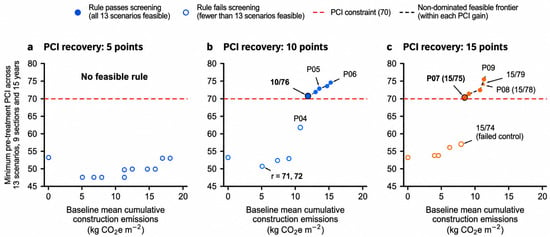
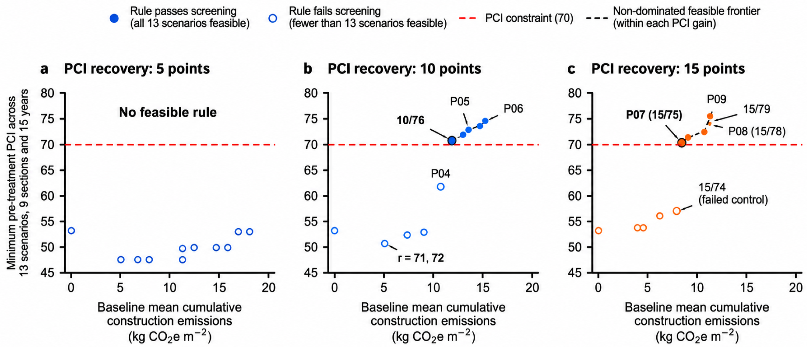
Under baseline parameters, 13 of the 33 rules kept pre-treatment PCI at or above 70 for every section and year. Eleven rules remained feasible in all 13 parameter scenarios, comprising five at a 10-point gain and six at a 15-point gain. No rule with a five-point gain was feasible. Differences in cumulative construction emissions followed differences in treatment counts because the per-event emission factor was fixed.

Figure 3 pairs baseline mean cumulative construction emissions with the lowest pre-treatment PCI across all nine sections, 15 years and 13 parameter scenarios. Filled markers denote rules feasible under all 13 parameter scenarios, whereas open markers denote rules that fail in at least one scenario. Within each assumed gain, changing the threshold altered treatment timing and counts as well as minimum pre-treatment PCI. Every modeled G event was assigned the same construction-stage inventory value, so the reported emission ranking followed the number of interventions. This comparison includes the adopted material-production, transport, mixing, and construction processes per event. It does not quantify changes in per-event emissions between construction sites or years, work-zone traffic effects, or later rehabilitation needs. Lower values in this comparison should therefore not be interpreted as whole-life carbon savings.

Figure 3. Baseline G-treatment emissions and minimum PCI across parameter scenarios.

4.2. Comparing Rules at a Fixed Gain

At an assumed 10-point PCI gain, a threshold of 76 was the lowest-emission rule that remained feasible in all 13 parameter scenarios. It scheduled 21 G events across the nine sections, with baseline mean cumulative construction emissions of 11.8677 $\mathrm{kg}{\mathrm{CO}}_2\mathrm{e}{\mathrm{m}}^{-2}$. The previously compared threshold of 78 scheduled 24 events and emitted 13.5631 $\mathrm{kg}{\mathrm{CO}}_2\mathrm{e}{\mathrm{m}}^{-2}$. Thus, the threshold of 76 reduced modeled emissions by 12.5% relative to 78 under the same assumed gain, while its worst-scenario minimum pre-treatment PCI was 70.8604.

At an assumed 15-point gain, threshold 75 was the lowest-emission rule that passed all 13 parameter scenarios. It scheduled 15 baseline G events across the nine sections, with mean cumulative construction emissions of 8.4770 $\mathrm{kg}{\mathrm{CO}}_2\mathrm{e}{\mathrm{m}}^{-2}$. Its worst-scenario minimum pre-treatment PCI was 70.3864, leaving a modeled margin of 0.3864 points. Threshold 74 had lower baseline emissions but failed the intermediate $\alpha -5\%$ test and was excluded. This 0.3864-point margin is a model-calculated scenario margin, not a safety allowance adjusted for PCI survey error or treatment-response variability. The selected threshold should not be applied as an operational rule without a locally specified condition buffer and field validation.

4.3. Sensitivity to Prescribed Deterioration-Parameter Perturbations

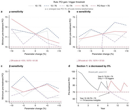
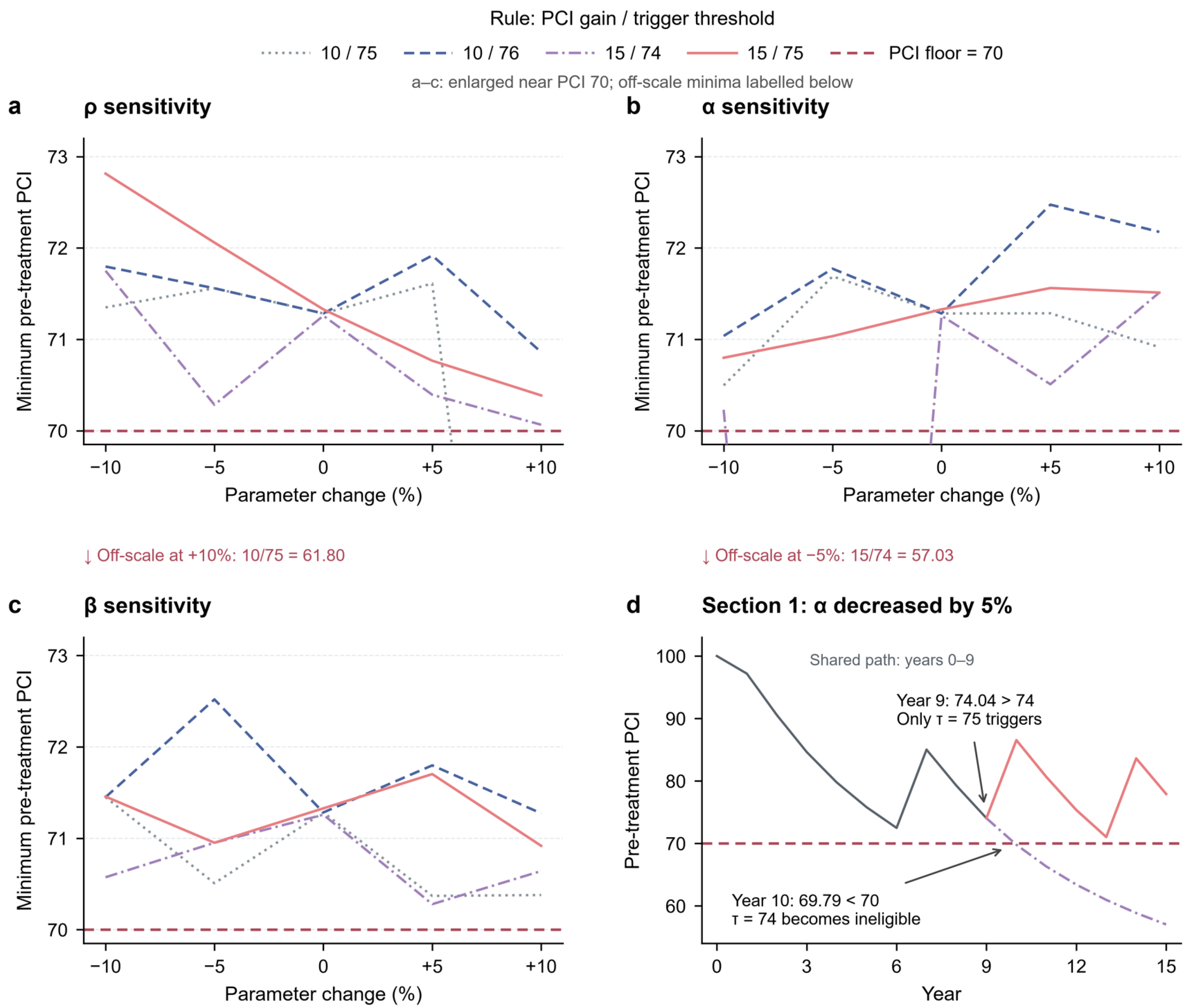
At a 10-point gain, five integer thresholds passed all 13 parameter scenarios. Figure 4 illustrates the sensitivity of maintenance rules to changes in the deterioration parameters. The threshold of 75 was feasible at baseline but failed when $\rho$ increased by 10%: section 1 fell below the G eligibility limit, and its PCI reached 61.8040 by year 15. The threshold of 76 passed all 13 scenarios; its lowest pre-treatment PCI was 70.8604, occurring on section 3 in year 12 when $\rho$ increased by 10%. Threshold 78 also passed all 13 scenarios but required three more baseline G events than threshold 76.

Figure 4. Sensitivity of maintenance rules to deterioration parameters.

At a 15-point gain, thresholds 75–80 passed all 13 parameter scenarios. Threshold 74 passed the endpoint tests but failed when $\alpha$ decreased by 5%. On section 1, PCI was 74.0419 in year 9, remaining above the trigger. It fell to 69.7931 in year 10, below the G eligibility limit, and reached 57.0349 in year 15. The rule therefore passed 12 of 13 scenarios and was excluded. This failure depends on the lower G-eligibility bound of PCI 70 imposed in the present model. Because the underlying PCI–RQI decision table lists G in some below-70 states, the result demonstrates failure of this restricted PCI-only rule, not that G is impossible below PCI 70 in practice.

This failure arose from the interaction between annual decisions, the trigger threshold and the lower treatment-eligibility limit. Adding intermediate perturbations changed the selected threshold from 74 to 75 at a 15-point gain. The result shows why passing perturbation endpoints does not establish feasibility at intervening parameter values. Raising the PCI floor to 71 selected threshold 77 at a 10-point gain and threshold 76 at a 15-point gain. Their baseline treatment counts were 23 and 16, with mean cumulative emissions of 12.9980 and 9.0421 $\mathrm{kg}{\mathrm{CO}}_2\mathrm{e}{\mathrm{m}}^{-2}$, respectively. Their lowest pre-treatment PCI values across the 13 scenarios were 71.9174 and 71.3919, respectively.

At a PCI 75 floor, no rule with a five- or ten-point assumed gain passed all 13 parameter scenarios. The only feasible rule had a 15-point gain and a trigger threshold of 80. It scheduled 20 G events across the nine sections under baseline parameters, giving mean cumulative construction emissions of 11.3026 $\mathrm{kg}{\mathrm{CO}}_2\mathrm{e}{\mathrm{m}}^{-2}$; its worst-scenario minimum pre-treatment PCI was 75.4824. This is a sensitivity result within the present G-only model, not a replication of the source study’s multi-treatment optimization. Table 4 summarizes the complete threshold sets that satisfied each specified PCI floor in all 13 parameter scenarios.

Table 4. Feasible integer PCI trigger thresholds by assumed treatment gain and pre-treatment PCI floor.

Minimum Pre-Treatment PCI Floor	Gain: 5 Points	Gain: 10 Points	Gain: 15 Points
70	None	76–80	75–80
71	None	77–80	76–80
75	None	None	80

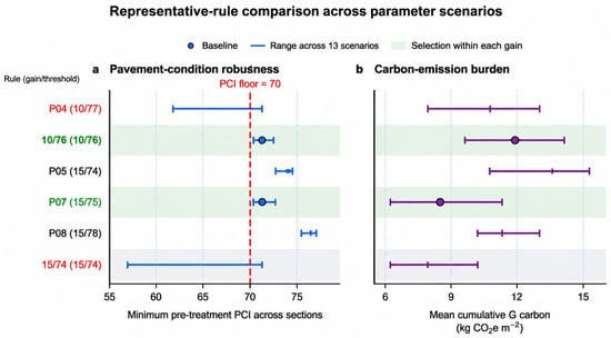
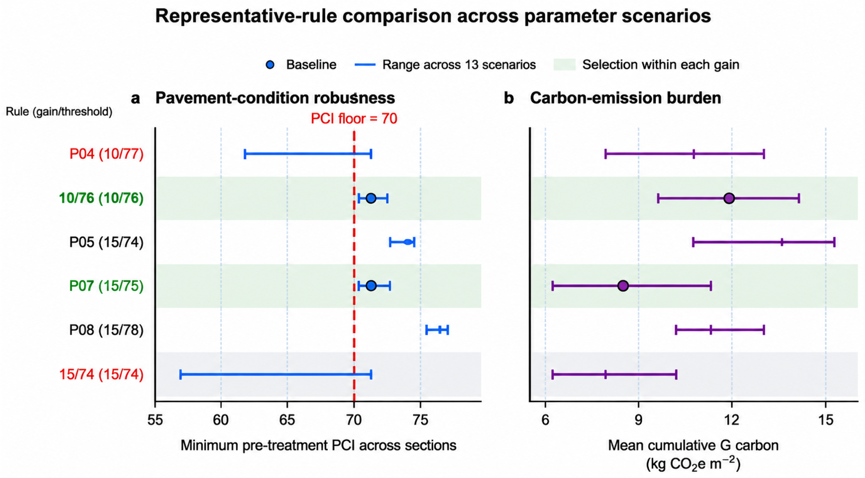
Figure 5 compares representative rules using baseline values and ranges across all 13 parameter scenarios. Dots show baseline results, and horizontal lines span scenario minima and maxima. These ranges are not statistical confidence intervals. P04 and 15/74 each failed one scenario, whereas 10/76 and P07 (15/75) passed all scenarios. The latter two rules were selected within their respective gain classes at the PCI 70 floor. Table 5 summarizes the baseline results and feasibility across parameter scenarios for the representative rules.

Figure 5. Ranges of pavement condition and carbon emissions for representative rules across parameter scenarios.

Table 5. Baseline and perturbed results for representative rules under the G eligibility constraint.

Rule	PCI Trigger Threshold	Assumed PCI Gain (Points)	Total G Events Across Nine Sections	Baseline Mean Cumulative Emissions	Baseline Minimum Pre-Treatment PCI	Feasible Scenarios at PCI $\ge 70$	Worst-Scenario Minimum Pre-Treatment PCI
P04	75	10	19	10.7375	71.2830	12/13	61.8040
10/76	76	10	21	11.8677	71.2830	13/13	70.8604
P05	78	10	24	13.5631	74.1046	13/13	72.8325
P06	80	10	27	15.2585	75.6941	13/13	74.5364
15/74	74	15	14	7.9118	71.2583	12/13	57.0349
P07	75	15	15	8.4770	71.3280	13/13	70.3864
P08	78	15	20	11.3026	73.9922	13/13	73.7478
P09	80	15	20	11.3026	76.4695	13/13	75.4824

Across the 13 scenarios, mean cumulative G emissions for P07 ranged from 6.2164 to 11.3026 $\mathrm{kg}{\mathrm{CO}}_2\mathrm{e}{\mathrm{m}}^{-2}$, versus 10.1723 to 12.9980 $\mathrm{kg}{\mathrm{CO}}_2\mathrm{e}{\mathrm{m}}^{-2}$ for P09. In every scenario, P07 had both lower cumulative emissions and a lower minimum pre-treatment PCI than P09. The emission–condition trade-off seen in Figure 5 thus persisted throughout the specified one-factor perturbation range, rather than appearing only under baseline parameters.

A common ±10% change in the per-event emission factor changed cumulative emissions proportionally without altering the selected thresholds. This scaling result applies to the common emission factor assumed here; it does not establish robustness to section-specific or schedule-dependent emissions. Table 6 reports the G treatment years for each section under three representative rules using baseline deterioration parameters.

Table 6. Section-wise G treatment years under representative rules with baseline deterioration parameters.

Section	10/76	15/75	15/80
1	6, 9, 11, 14	6, 10, 13	5, 8, 11, 15
2	7, 10, 13, 15	8, 12	5, 9, 13
3	6, 9, 12, 15	7, 11, 15	5, 9, 13
4	7, 10, 13	8, 12	6, 10, 14
5	10, 15	10	8, 14
6	13	14	10
7	9, 13	9, 15	7, 12
8	13	14	11
9	–	–	13
Total G events	21	15	20

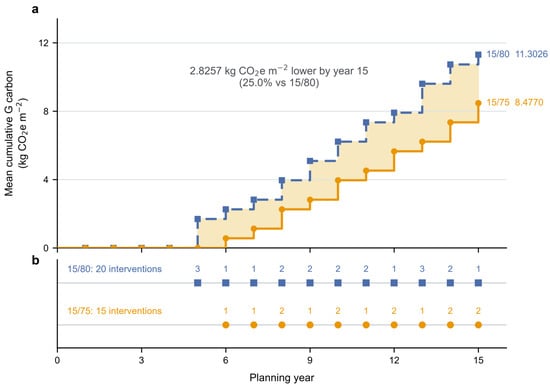
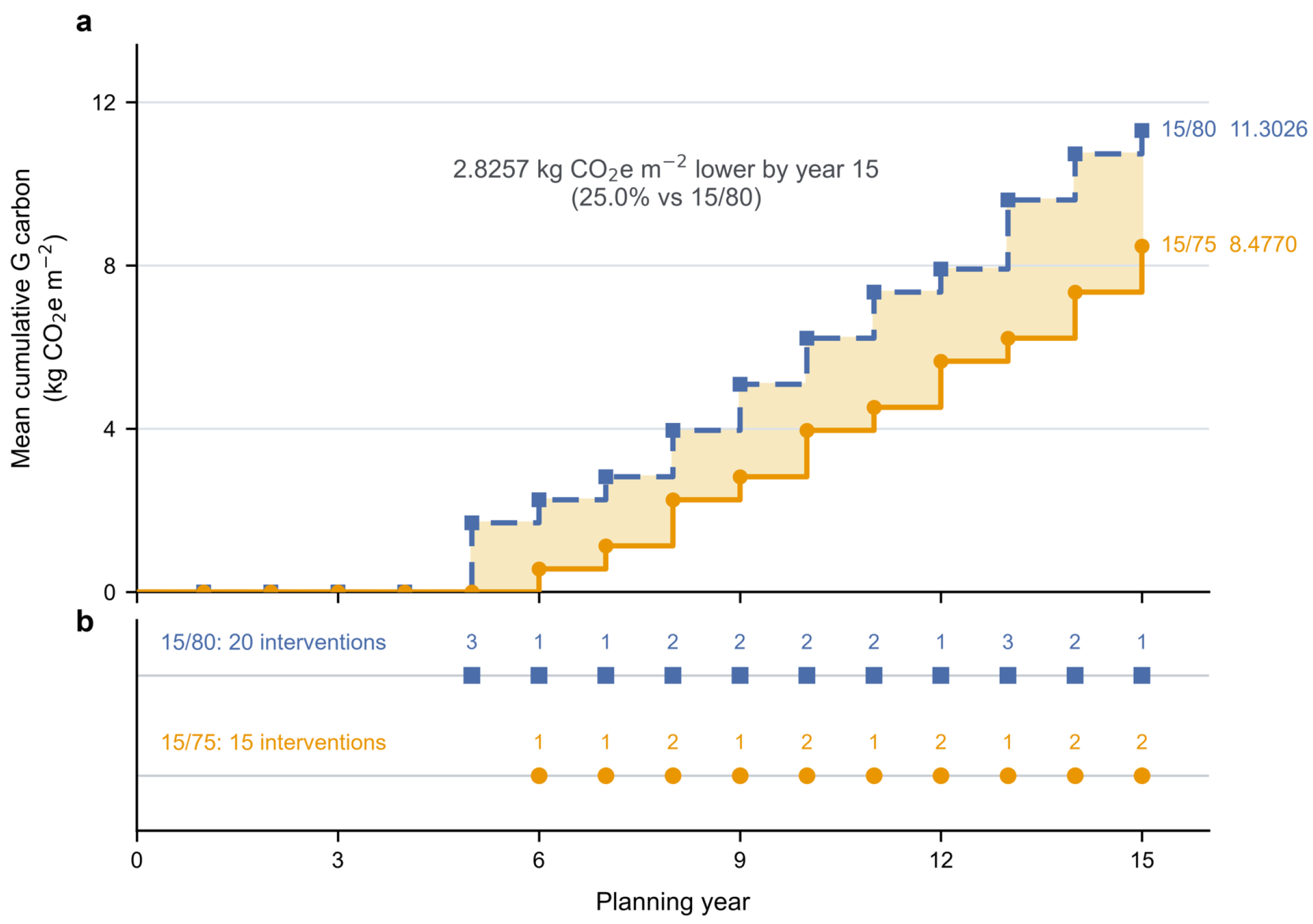
Figure 6 compares baseline schedules for the 15/75 and 15/80 (P09) rules across the nine sections. The 15/75 rule scheduled 15 G events, compared with 20 for 15/80 over the 15-year horizon. Their mean cumulative construction emissions were 8.4770 and 11.3026 $\mathrm{kg}{\mathrm{CO}}_2\mathrm{e}{\mathrm{m}}^{-2}$, respectively. With the same fixed emission factor applied to every G event, the 25.0% difference between 15/75 and 15/80 follows from five fewer modeled interventions (15 versus 20) within the specified four-stage inventory boundary. It does not establish net life-cycle greenhouse-gas savings. On section 1, the corresponding treatment years were 6, 10 and 13 versus 5, 8, 11 and 15. Section 9 received no treatment under 15/75 but was treated in year 13 under 15/80.

Figure 6. Construction emissions and treatment timing for the 15/75 and 15/80 rules: (a) mean cumulative construction emissions over the planning horizon; (b) timing and number of G treatment events across the nine sections. emissions and treatment timing for 15/75 and 15/80.

At the fixed direct construction cost of CNY 57.3846 ${\mathrm{m}}^{-2}$ per event, mean cumulative costs were CNY 95.6410 and 127.5213 ${\mathrm{m}}^{-2}$, respectively. Cost was proportional to treatment count and was reported as a secondary outcome rather than a selection criterion.

4.4. Discussion

Under a common per-event emission factor, the modeled emission advantage of a maintenance rule arose from fewer interventions. P08 and P09 incurred equal emissions but differed in minimum and year-15 PCI. Emission totals therefore required interpretation alongside pavement condition and the specified performance floor. This comparison concerns the adopted construction-emission boundary and does not quantify traffic-disruption emissions or other schedule-dependent effects.

The intermediate-perturbation failure of 15/74 shows that endpoint screening can miss changes in treatment eligibility. Annual decisions allow PCI to move from above the trigger to below the eligibility interval between successive inspections. The selected threshold therefore depends on the assumed treatment gain, deterioration parameters and required performance floor. Feasibility across the tested scenarios does not guarantee feasibility throughout the continuous parameter range or establish operational reliability.

The selected rules remain conditional on adopted deterioration parameters and assumed treatment gains. Initial PCI was fixed, and deterioration parameters were reused after successive G events without validation against observed repeated treatments. The twelve one-parameter perturbations assess prescribed scenarios rather than confidence limits or simultaneous uncertainty. RQI and variation in traffic loading were not modeled, and equal section weighting does not represent a Xinjiang-wide network estimate. Field application requires longitudinal validation of deterioration and treatment response, together with an operational condition margin.

5. Conclusions

This study linked PCI-triggered maintenance scheduling to cumulative construction emissions while enforcing section-wise pavement-condition constraints over a 15-year horizon. Under the common per-event emission factor, lower emissions followed fewer interventions. Performance screening was therefore essential for separating admissible schedules from rules that reduced emissions by allowing unacceptable condition deterioration.

Adding intermediate parameter perturbations changed the feasible-rule set. The 15-point-gain threshold of 74 passed the ±10% endpoint tests but failed when $\mathsf{\alpha }$ decreased by 5%. This case shows that endpoint checks can miss failures created by discrete treatment decisions and eligibility limits. The 13-scenario screen selected thresholds 76 and 75 at assumed gains of 10 and 15 points, respectively.

The selected rules also depended on the required condition margin. Raising the PCI floor from 70 to 71 changed the selected thresholds to 77 and 76, respectively. Threshold selection should therefore be conditional on achievable treatment gains and explicit service-level requirements, rather than expressed as a universal numerical recommendation. The broader implication is that maintenance thresholds should be screened against treatment eligibility and section-wise condition requirements, including intermediate parameter values when decisions are discrete. The numerical thresholds obtained here remain conditional on the nine section parameter sets, assumed treatment gains and construction-emission boundary. Future research should validate deterioration and repeated-treatment response using longitudinal observations and examine joint parameter variation, condition-measurement uncertainty and schedule-dependent emissions.

References

- Liu, N.; Wang, Y.; Bai, Q.; Liu, Y.; Wang, P.; Xue, S.; Yu, Q.; Li, Q. Road life-cycle carbon dioxide emissions and emission reduction technologies: A review. J. Traffic Transp. Eng. (Engl. Ed.) 2022, 9, 532–555. [Google Scholar] [CrossRef] [Scilit]
- Liljenström, C.; Björklund, A.; Toller, S. Including maintenance in life cycle assessment of road and rail infrastructure—A literature review. Int. J. Life Cycle Assess. 2022, 27, 316–341. [Google Scholar] [CrossRef] [Scilit]
- Liu, Z.; Balieu, R.; Kringos, N. Integrating sustainability into pavement maintenance effectiveness evaluation: A systematic review. Transp. Res. Part D Transp. Environ. 2022, 104, 103187. [Google Scholar] [CrossRef] [Scilit]
- Mao, J.; Zhu, Y.; Chen, Q.; Yu, H. Energy Consumption and Carbon Emission Analysis of Typical Regeneration Methods for Asphalt Pavements. Buildings 2023, 13, 1569. [Google Scholar] [CrossRef] [Scilit]
- de Bortoli, A.; Baouch, Y.; Masdan, M. BIM can help decarbonize the construction sector: Primary life cycle evidence from pavement management systems. J. Clean. Prod. 2023, 391, 136056. [Google Scholar] [CrossRef] [Scilit]
- Zhang, L.; Tian, W.; Wang, B.; Dai, X. Dynamic Life Cycle Assessment of Low-Carbon Transition in Asphalt Pavement Maintenance: A Multi-Scale Case Study Under China’s Dual-Carbon Target. Sustainability 2025, 17, 6540. [Google Scholar] [CrossRef] [Scilit]
- Li, J.; Pitt, M.; Ma, L.; Jia, J.; Jiang, F. A multi-objective differential evolutionary algorithm for optimal sustainable pavement maintenance plan at the network level. J. Clean. Prod. 2022, 381, 135212. [Google Scholar] [CrossRef] [Scilit]
- Guan, X.; Zhang, H.; Du, X.; Zhang, X.; Sun, M. An Improved Method for Optimizing the Timing of Preventive Maintenance of Pavement: Integrating LCA and LCCA. Appl. Sci. 2023, 13, 10629. [Google Scholar] [CrossRef] [Scilit]
- Chen, W.; Zheng, M.; Tian, N.; Ding, X.; Li, N.; Zhang, W. Project-based sustainable timing series decision-making for pavement maintenance using multi-objective optimization: An innovation in traditional solutions. J. Clean. Prod. 2023, 407, 137172. [Google Scholar] [CrossRef] [Scilit]
- Yao, L.; Leng, Z.; Jiang, J.; Ni, F. Large-Scale Maintenance and Rehabilitation Optimization for Multi-Lane Highway Asphalt Pavement: A Reinforcement Learning Approach. IEEE Trans. Intell. Transp. Syst. 2022, 23, 22094–22105. [Google Scholar] [CrossRef] [Scilit]
- Liu, S.-S.; Arifin, M.F.A.; Chen, W.T. An Integrated Optimization Model for Life Cycle Pavement Maintenance Budgeting Problems. IEEE Access 2022, 10, 13884–13900. [Google Scholar] [CrossRef] [Scilit]
- Chen, L. Network-level pavement maintenance and rehabilitation decision-making with the optimized annual budget. PLoS ONE 2023, 18, e0287426. [Google Scholar] [CrossRef] [Scilit]
- Philip, B.; AlJassmi, H. A Bayesian decision support system for optimizing pavement management programs. Heliyon 2024, 10, e25625. [Google Scholar] [CrossRef] [Scilit]
- Yao, L.; Leng, Z.; Jiang, J.; Ni, F. A multi-agent reinforcement learning model for maintenance optimization of interdependent highway pavement networks. Comput.-Aided Civ. Infrastruct. Eng. 2024, 39, 2951–2970. [Google Scholar] [CrossRef] [Scilit]
- Wang, Z.; Yang, L.; Ranyal, E.; Briessinck, M.; Eckelman, M.J.; Cao, Z.; Hernando, D. Computational optimization for low-carbon and circular pavement management at the network level. Resour. Conserv. Recycl. 2026, 225, 108636. [Google Scholar] [CrossRef] [Scilit]
- Ali, A.; Heneash, U.; Hussein, A.; Eskebi, M. Predicting Pavement Condition Index Using Fuzzy Logic Technique. Infrastructures 2022, 7, 91. [Google Scholar] [CrossRef] [Scilit]
- Zhang, Y.; D’avigneau, A.M.; Hadjidemetriou, G.M.; de Silva, L.; Girolami, M.; Brilakis, I. Bayesian dynamic modelling for probabilistic prediction of pavement condition. Eng. Appl. Artif. Intell. 2024, 133, 108637. [Google Scholar] [CrossRef] [Scilit]
- Alonso-Solorzano, Á.; Pérez-Acebo, H.; Findley, D.J.; Gonzalo-Orden, H. Transition probability matrices for pavement deterioration modelling with variable duty cycle times. Int. J. Pavement Eng. 2023, 24, 2278694. [Google Scholar] [CrossRef] [Scilit]
- Zhang, C.; Tan, Y.; Gao, Y.; Fu, Y.; Li, J.; Li, S.; Zhou, X. Resilience assessment of asphalt pavement rutting under climate change. Transp. Res. Part D Transp. Environ. 2022, 109, 103395. [Google Scholar] [CrossRef] [Scilit]
- Li, J.; He, W.; Cheng, H.; Wang, H. A streamlined approach for probabilistic pavement life-cycle performance prediction via physics-informed neural networks. Comput.-Aided Civ. Infrastruct. Eng. 2025, 40, 5136–5152. [Google Scholar] [CrossRef] [Scilit]
- Chowdhury, L.F.; Guler, S.I.; Stoffels, S.M. Multi-objective optimization of maintenance, repair, and rehabilitation schedule for pavements in urban networks considering greenhouse gas emissions. Struct. Infrastruct. Eng. 2025, 1–15. [Google Scholar] [CrossRef] [Scilit]
- Bai, S.; Varga, L.; Manola, E. Unexplored challenges in quantifying and reducing carbon emissions in road maintenance. Transp. Res. Part A Policy Pract. 2026, 204, 104844. [Google Scholar] [CrossRef] [Scilit]
- Suwarto, F.; Parry, T.; Airey, G. Review of methodology for life cycle assessment and life cycle cost analysis of asphalt pavements. Road Mater. Pavement Des. 2024, 25, 1631–1657. [Google Scholar] [CrossRef] [Scilit]
- Abed, A.; Bizarro, D.E.G.; Neves, L.; Parry, T.; Keijzer, E.; Presti, D.L.; Kalman, B.; Carrion, A.J.D.B.; Mantalovas, K.; Buttitta, G.; et al. Uncertainty analysis of life cycle assessment of asphalt surfacings. Road Mater. Pavement Des. 2024, 25, 219–238. [Google Scholar] [CrossRef] [Scilit]
- Bo, W.; Qian, Z.; Yu, B.; Ren, H.; Yang, C.; Zhao, K.; Zhang, J. MILP-Based Approach for High-Altitude Region Pavement Maintenance Decision Optimization. Appl. Sci. 2024, 14, 7670. [Google Scholar] [CrossRef] [Scilit]
- García-Segura, T.; Montalbán-Domingo, L.; Llopis-Castelló, D.; Sanz-Benlloch, A.; Pellicer, E. Integration of deep learning techniques and sustainability-based concepts into an urban pavement management system. Expert Syst. Appl. 2023, 231, 120851. [Google Scholar] [CrossRef] [Scilit]
- Naseri, H.; Aliakbari, A.; Javadian, M.A.; Waygood, E. A novel technique for multi-objective sustainable decisions for pavement maintenance and rehabilitation. Case Stud. Constr. Mater. 2024, 20, e03037. [Google Scholar] [CrossRef] [Scilit]
- Al-Mansour, A.; Lee, K.-W.W.; Al-Qaili, A.H. Prediction of Pavement Maintenance Performance Using an Expert System. Appl. Sci. 2022, 12, 4802. [Google Scholar] [CrossRef] [Scilit]
- Cano-Ortiz, S.; Pascual-Muñoz, P.; Castro-Fresno, D. Machine learning algorithms for monitoring pavement performance. Autom. Constr. 2022, 139, 104309. [Google Scholar] [CrossRef] [Scilit]
- Xu, X.; Wang, S.; Kang, F.; Li, S.; Li, Q.; Wu, T. Multi-Attribute Decision-Making Method in Preventive Maintenance of Asphalt Pavement Based on Optimized Triangular Fuzzy Number. Sustainability 2024, 16, 2787. [Google Scholar] [CrossRef] [Scilit]
- JTG/T 5142-01–2021; Technical Specifications for Preventive Maintenance of Highway Asphalt Pavement. China Communications Press: Beijing, China, 2021. (In Chinese)
Disclaimer/Publisher’s Note: The statements, opinions and data contained in all publications are solely those of the individual author(s) and contributor(s) and not of MDPI and/or the editor(s). MDPI and/or the editor(s) disclaim responsibility for any injury to people or property resulting from any ideas, methods, instructions or products referred to in the content. |
© 2026 by the authors. Licensee MDPI, Basel, Switzerland. This article is an open access article distributed under the terms and conditions of the Creative Commons Attribution (CC BY) license.