Evidence-Gated Symbolic Correction for Data-Limited Geomechanical Models

Featured Application

Assessment of explicit corrections to existing rock-mechanics models when measurements are limited, including physical screening before constitutive implementation and identification of cases requiring additional observations.

Abstract

Geomechanical models often retain systematic errors after calibration, but sparse observations may support several competing corrections. We present an evidence-gated symbolic regression framework that retains an existing baseline and evaluates explicit corrections using coefficient fitting, grouped validation, and physical checks. Evolutionary search and optional large language model proposals supply candidates to a common evaluator. Additional observations are requested only when admissible candidates make sufficiently different predictions; unresolved corrections remain provisional. Across 32 cases covering four nonlinear response families and eight previously unused data seeds, predictive-disagreement sampling reduced mean normalized held-out RMSE from 0.193 without acquisition to 0.117. A fixed-budget comparison showed that gating saved 28.1% of space-filling observations at an increase of 0.028 in normalized RMSE. Controlled weak-plane tests verified constitutive-law recovery and FLAC3D material-point implementation. In a separate numerical demonstration of staged cavern excavation, a transferred cohesion-decay correction reduced multi-response RMSE against a prescribed reference from 2.24 to 0.694 mm. Grouped evaluation of four published rock datasets supported two corrections and retained two as provisional. The framework assesses predictive improvement, physical admissibility, and evidence sufficiency without equating a good fit with recovery of the governing equation.

1. Introduction

Rock-mechanics models are used to interpret laboratory tests and predict the response of underground excavations. Their constitutive assumptions and calibrated parameters may capture the dominant behavior while leaving systematic errors associated with anisotropy, state dependence, or scale. An explicit correction can preserve the useful part of an existing model and represent behavior that the baseline does not explain. This approach is related to model discrepancy and hybrid modeling [1,2]. For engineering use, however, reducing fitting error is only part of the problem: the correction must also satisfy relevant physical restrictions and have support from observations beyond those used to fit its coefficients.

This study concerns problems with an operational baseline and a comparatively low-dimensional discrepancy. It does not attempt to infer a complete history-dependent constitutive model from raw data. Neural and physics-informed constitutive approaches address broader representation problems [3,4,5,6]; here, the objective is an explicit modification that can be inspected and, where appropriate, implemented in an existing solver. Additional evidence may come from laboratory measurements or numerical evaluations. When such observations cannot be obtained, the method must still distinguish a supported correction from one that remains uncertain.

Symbolic regression searches mathematical expressions directly and is therefore well suited to explicit model correction. Free-form discovery, sparse identification, physics-inspired search, and neural approaches have broadened its capabilities [7,8,9,10,11]. In geomechanics, interpretable regression has been used for sparse-data constitutive modeling, anisotropic tunnel closure, and physically informed constitutive or governing-equation discovery [12,13,14,15]. Nevertheless, performance depends on the operator set, fitting procedure, data coverage, and search budget [16,17]; the underlying search is computationally difficult [18].

Limited observations introduce a second difficulty even when suitable expressions are generated. Several physically admissible corrections may fit nearly equally well over the measured range yet predict different behavior at other stresses, orientations, or states. Validation folds drawn from the same restricted range may not resolve these alternatives. Model-discrimination experiments and Bayesian experimental design select observations to distinguish competing explanations [19,20], while information-based active learning exploits predictive disagreement [21]. For symbolic correction, both the expressions and their coefficients vary, so deciding whether more evidence is needed should be distinguished from choosing where to collect it.

Large language models (LLMs) provide another source of candidate expressions. Recent methods combine their proposals with numerical optimization and iterative feedback [22,23,24]. Such proposals may broaden a search but do not themselves establish mechanical plausibility or predictive validity. We therefore treat the LLM as an optional candidate generator, applying the same fitting, validation, and physical checks to all retained expressions. This keeps the acceptance decision independent of how a candidate was proposed.

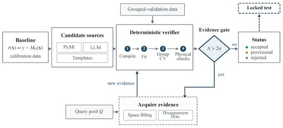
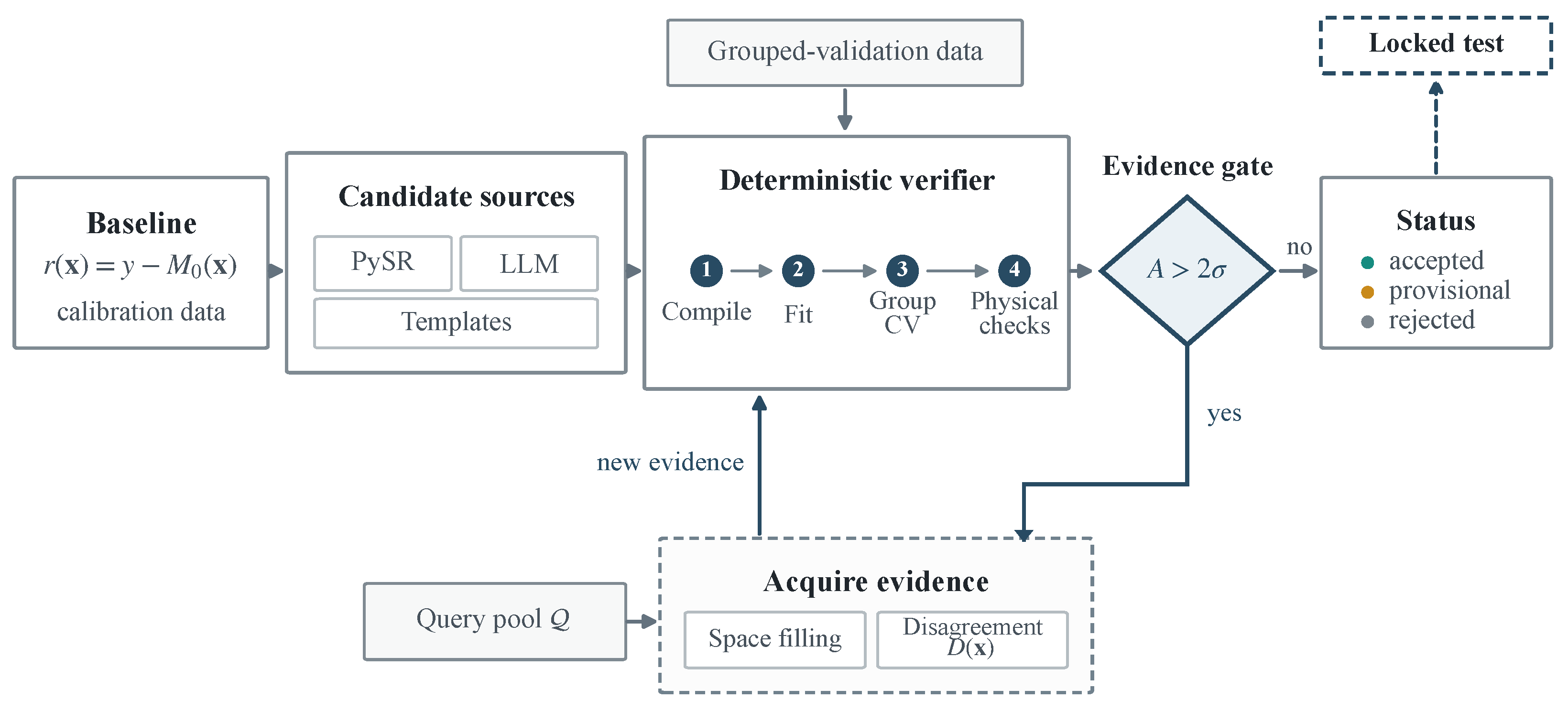
We introduce an evidence-gated framework for this setting. Explicit additive or multiplicative corrections and replacements of declared components are evaluated against the unchanged baseline. The contribution is an explicit decision rule connecting ambiguity among admissible corrections to the acquisition of further observations and to the status assigned to a correction. It separates whether more evidence is needed from where to collect it. Candidate generators and query-ranking policies can be changed while retaining the same evidence requirements. The gate requests observations only when near-equivalent candidates differ beyond a specified noise-scaled threshold; insufficiently supported corrections remain provisional. Figure 1 summarizes the procedure.

Figure 1. Evidence-gated symbolic correction of an existing model. Candidate expressions undergo the same fitting, validation, and physical checks. Additional observations are requested when at least two near-equivalent admissible candidates disagree beyond the noise-scaled threshold; the available evidence then determines an accepted, provisional, or rejected outcome. Held-out test responses are evaluated after the correction and its status have been fixed. Teal, amber, and gray dots denote accepted, provisional, and rejected status, respectively. Solid arrows show the evaluation and acquisition flow; dashed outlines mark conditional acquisition and the isolated locked test, linked to the fixed status by a dashed arrow.

The evaluation separates questions that are often conflated. A 32-case study measures the predictive effect of conditional acquisition under sparse evidence. Controlled weak-plane tests assess constitutive recovery and FLAC3D implementation consistency; a separate cavern calculation demonstrates propagation of a fixed correction through staged excavation. Four published rock datasets test whether corrections improve grouped validation. These studies report prediction, structural recovery, physical admissibility, and numerical transfer separately. Section 2 defines the method, Section 3 and Section 4 present the evaluations, and Section 5 and Section 6 discuss engineering use and conclusions.

2. Evidence-Gated Symbolic Model Correction

The method starts with a model already in use and compares several explicit ways to correct it. Each proposed correction is fitted to the available observations and checked against the required physical properties. If several corrections fit similarly well but predict different responses, the method requests an observation that can help to distinguish them. It then refits and checks the corrections again. A correction is accepted only when the evidence and physical checks support it; otherwise, it remains provisional or is rejected. Additional observations are therefore requested to resolve a specific uncertainty, rather than simply to exhaust a measurement budget.

2.1. Problem Formulation and Evidence Partitioning

For an observation pair $(\mathit{x},y)$, let $M_0\left(\mathit{x}\right)$ denote the corresponding baseline prediction. The residual measures the part of the observed response that the baseline does not explain:

$$r\left(\mathit{x}\right)=y-M_0\left(\mathit{x}\right),$$

(1)

where $\mathit{x}$ may contain orientation, stress, temperature, loading-rate, or state variables. The objective is not to replace $M_0$ but to construct a corrected model $M\left(\mathit{x}\right)$ whose departure from the baseline is explicit and inspectable.

Each experiment assigns observations to four roles. The calibration set is used to fit continuous coefficients. Grouped cross-validation (Group-CV) compares expressions without splitting correlated observations from the same angle, loading path, or data realization. The query pool contains locations where an additional response can be acquired if structural ambiguity is detected. The locked test set is evaluated only after model selection and is unavailable to candidate generation, coefficient fitting, acquisition, stopping, and acceptance. Access to locked responses is disabled throughout these stages, including LLM-based candidate generation.

Algorithm 1 summarizes the workflow. Multiple candidate sources and additional data acquisition are optional; typed validation, deterministic evaluation, physical verification, and isolation of the locked test set are required.

Algorithm 1 Evidence-gated symbolic model correction

Require: Baseline $M_0$; calibration data ${\mathcal{D}}_{\mathrm{cal}}$; grouped validation data ${\mathcal{D}}_{\mathrm{cv}}$; query pool $\mathcal{Q}$; locked data ${\mathcal{D}}_{\mathrm{lock}}$; admissibility criteria $\mathcal{C}$ and verification domain $\mathsf{\Omega }$; observation-noise scale $\sigma$; acquisition policy and budget B Ensure: Correction status (accepted, provisional, or rejected), structural-ambiguity flag, selected candidate if applicable, and an analysis record 1: Compute residual diagnostics from $M_0$ using visible data only 2: Propose typed corrections using PySR, optional LLM proposals, and applicable provenance-tracked templates 3: for each proposed correction q do 4:       Check q against the permitted variables, operators, expression depth, and domain restrictions 5:       Fit its coefficients on ${\mathcal{D}}_{\mathrm{cal}}$ and evaluate grouped error on ${\mathcal{D}}_{\mathrm{cv}}$ 6:       heck physical behavior and numerical stability over $\mathsf{\Omega }$ 7: end for 8: Rank the admissible correction candidates together with the null baseline candidate $q_0$, and construct ${\mathcal{E}}_{ϵ}$ 9: while $|{\mathcal{E}}_{ϵ}| \ge 2$, $A\left({\mathcal{E}}_{ϵ}\right)>2\sigma$, $\mathcal{Q}\ne ⌀$, and fewer than B points have been acquired do 10:     Select ${\mathit{x}}^{\ast }\in \mathcal{Q}$ with the prespecified acquisition policy 11:     Acquire $y\left({\mathit{x}}^{\ast }\right)$, append it to ${\mathcal{D}}_{\mathrm{cal}}$, remove ${\mathit{x}}^{\ast }$ from $\mathcal{Q}$, and refit and reverify all eligible candidates 12:     Reconstruct ${\mathcal{E}}_{ϵ}$ and reevaluate the ambiguity gate 13: end while 14: Record whether meaningful structural ambiguity remains 15: Apply the acceptance criteria; retain an admissible but insufficiently supported candidate as provisional, or report rejection if none remains 16: Evaluate ${\mathcal{D}}_{\mathrm{lock}}$ only after the selected candidate, fitted coefficients, and correction status have been fixed; report prediction, response adequacy, structure, and verifier outcomes separately

2.2. Typed Corrections and Candidate Generation

A correction proposal is represented by the tuple

$$q=(e,\mathcal{T},\mathcal{S},\pi ),$$

where e is a typed expression tree, $\mathcal{T}$ identifies how the expression modifies the baseline, $\mathcal{S}$ specifies its physical scope and domain restrictions, and $\pi$ records provenance. Three correction operators are retained. An additive correction supplies a missing contribution to the predicted response:

$$M_{\mathrm{add}}\left(\mathit{x}\right)=M_0\left(\mathit{x}\right)+e(\mathit{x};\mathit{\theta }),$$

(2)

A multiplicative correction changes the baseline response in proportion to its current value:

$$M_{\mathrm{mult}}\left(\mathit{x}\right)=M_0\left(\mathit{x}\right)\left[1+e(\mathit{x};\mathit{\theta })\right],$$

(3)

A replacement correction changes a specified component of the model when an output-level adjustment is insufficient:

$$M_{\mathrm{replace}}\left(\mathit{x}\right)=\mathcal{P}\left(M_0,e(\mathit{x};\mathit{\theta }),\mathcal{T}\right),$$

(4)

where $\mathcal{P}$ replaces a declared model subtree or constitutive component rather than adding an output-level residual. Typing refers to the declared edit operator, target, variables, and expression grammar; it is not an automated dimensional-analysis system. The problem specification must therefore provide nondimensionalized or otherwise unit-consistent variables and targets. Variables, parameters, and operators are checked recursively against that specification. Expressions that exceed the permitted depth, refer to unavailable state variables, violate the declared type restrictions, or fail finite-domain checks are rejected before fitting.

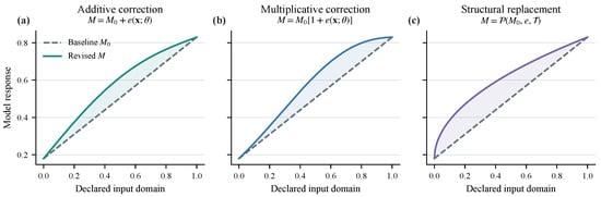
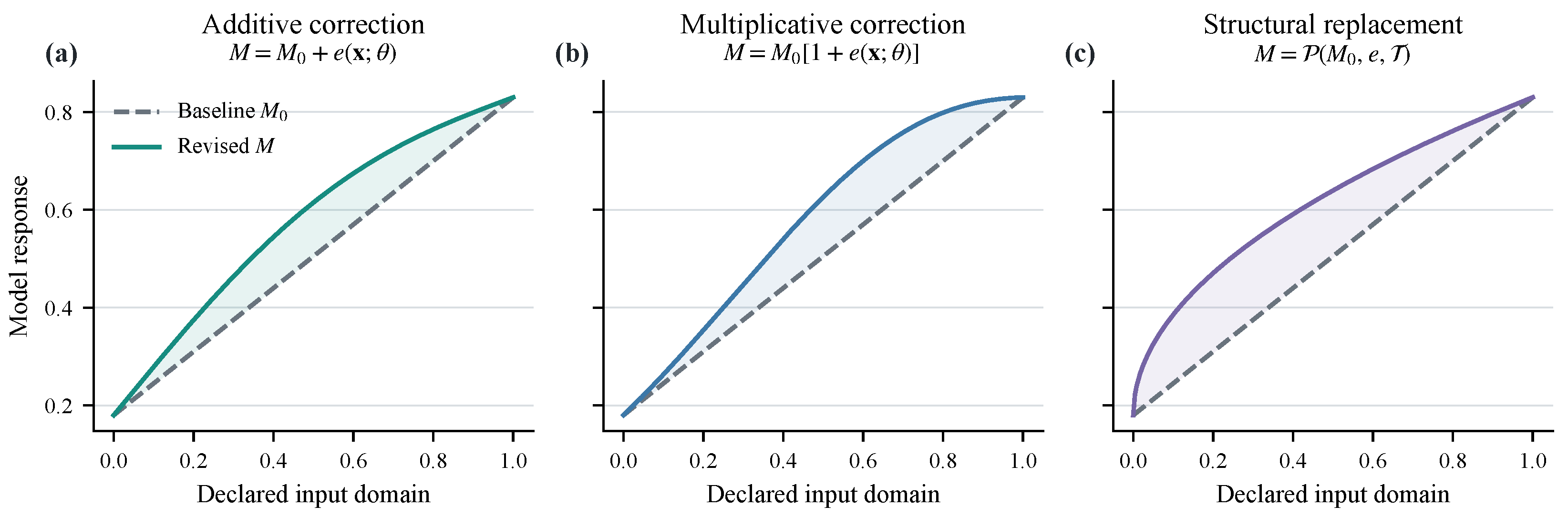
Figure 2 illustrates the three correction operators.

Figure 2. Baseline-aware typed correction algebra: (a) additive residual correction, (b) multiplicative correction, and (c) replacement of a declared model subtree.

The representation distinguishes expressive coverage from selection. A correct family may be permitted by the correction algebra without being generated, and it may be generated without being distinguishable from an alternative on the available observations. Candidate coverage and final recovery are therefore reported separately.

The candidate pool can combine three sources. PySR performs evolutionary symbolic regression with a declared operator set and search budget [17]. Provenance-tracked domain templates contribute only when their variables and physical scope match the problem specification. An LLM can propose typed expression trees from the baseline description, visible observations, residual diagnostics, and a compact set of curated domain relations. It does not receive the hidden reference equation or locked-test responses.

LLM proposals enter the candidate set only after they satisfy the same typed representation and domain restrictions as other expressions. Malformed proposals are rejected; syntactic normalization is permitted only when the mathematical content is unchanged. All retained candidates then undergo identical coefficient fitting and verification. Candidate budgets, visible data, fitting seeds, and verifier settings are recorded so that candidate sources can be compared under the same evaluation procedure; reproducibility settings are given in Supplementary Table S4.

2.3. Deterministic Verification and Structural Ambiguity

Coefficients $\mathit{\theta }$ are fitted by nonlinear least squares or regularized linear fitting, depending on the expression. For literature and loading-path cases, validation withholds complete groups to assess prediction beyond the fitted paths or orientations:

$$E_{\mathrm{cv}}\left(q\right)={\left[{\displaystyle \frac{1}{N}}\sum _{g\in \mathcal{G}}\sum _{i\in g}{\left(y_i-M_{q,-g}\left({\mathit{x}}_i\right)\right)}^2\right]}^{1/2},$$

(5)

where $\mathcal{G}$ is the collection of held-out groups, $M_{q,-g}$ is fitted without group g, and $N={\sum }_{g\in \mathcal{G}}\left|g\right|$ counts the held-out observations across folds. A group contains a complete orientation, loading path, or data realization. The 32-case evaluation instead fits coefficients on a fixed calibration subset and evaluates them on three validation environments, without leave-environment-out refitting. In that design, $E_{\mathrm{cv},h}\left(q\right)$ is the RMSE in environment h using the same fitted coefficients. Supplementary Tables S3 and S4 give the partitions and environment construction.

The verifier evaluates criteria $\mathcal{C}={\left\{C_j\right\}}_{j=1}^J$ over a declared verification domain $\mathsf{\Omega }$. Depending on the problem, these criteria can include finite output, positivity, bounded residual magnitude, admissible parameter signs, monotonicity, endpoint behavior, saturation, non-negative dissipation, or stable state evolution. Each criterion must follow from the physical assumptions of the baseline or documented domain knowledge. The violation vector is

$$v\left(q\right)=\left[v_1\left(q\right),\dots ,v_J\left(q\right)\right],v_j\left(q\right)=\mathbb{I}\left[C_j(M_q,\mathsf{\Omega })=\mathrm{false}\right].$$

(6)

Candidates are classified as admissible when ${\sum }_j{v}_j=0$. The numerical implementation checks the required physical constraints at specified input points within $\mathsf{\Omega }$; passing these checks does not prove that the constraints hold throughout the domain. Supplementary Section S15 gives the point-selection rules, tolerances, and results of an independent check on a finer grid. Among admissible candidates in the one-standard-error set defined below, the selection rule favors lower complexity and stable extrapolation. A lower RMSE cannot override a violation of a required physical constraint.

For a fitted correction intended for use over a continuous input range, verification can be strengthened without collecting new observations. The complete corrected expression, rather than its residual alone, is differentiated to check the required monotonicity directions. Where symbolic signs or interval bounds establish a constraint over a region, that region needs no further subdivision. Otherwise, the region is bisected and checked again until the constraint is established, a violating point is found, or the verification budget is reached. A budget-limited check remains undetermined, not proved. Supplementary Section S15 specifies this procedure and applies it to the fixed fitted corrections; the original prediction comparisons are unchanged.

For the 32-case evaluation, the validation risk measures performance in the least well-predicted of the three environments:

$$R_{\mathrm{cv}}\left(q\right)=\underset{h\in \{1,2,3\}}{\max }{E}_{\mathrm{cv},h}\left(q\right).$$

(7)

The unchanged baseline participates as a null candidate $q_0$. Let $q^{†}$ minimize the risk among $q_0$ and admissible corrections. The near-equivalent set retains expressions within one estimated standard error of this minimum:

$${\mathcal{E}}_{ϵ}=\left\{q:\sum _j{v}_j\left(q\right)=0,R_{\mathrm{cv}}\left(q\right)\le R_{\mathrm{cv}}\left(q^{†}\right)+{ϵ}_E\right\}.$$

(8)

Here, ${ϵ}_E$ is one standard error of the RMSE of $q^{†}$ in its worst environment, calculated as specified in Supplementary Section S2. It is case-dependent and is not tuned from held-out outcomes. The representative is selected by complexity, parameter count, risk, extrapolation amplification, and a fixed source-independent ordering (Supplementary Table S3). The gate decides whether another observation is warranted by comparing the largest prediction difference between retained candidates with the measurement-noise scale. This difference is measured as the largest pairwise prediction RMSE over the query pool:

$$A\left({\mathcal{E}}_{ϵ}\right)=\underset{\begin{array}{c}q,q^{\prime }\in {\mathcal{E}}_{ϵ}\\ q\ne q^{\prime }\end{array}}{\max }{\left[{\displaystyle \frac{1}{\left|\mathcal{Q}\right|}}\sum _{\mathit{x}\in \mathcal{Q}}{\left(M_q\left(\mathit{x}\right)-M_{q^{\prime }}\left(\mathit{x}\right)\right)}^2\right]}^{1/2},$$

(9)

where $\mathcal{Q}$ is the nonempty remaining query pool. The gate triggers when $|{\mathcal{E}}_{ϵ}| \ge 2$ and $A\left({\mathcal{E}}_{ϵ}\right)>2\sigma$, with the family-specific measurement-noise scale $\sigma$ given in Supplementary Table S1. Once an observation is warranted, the weighted prediction spread identifies locations where the plausible corrections disagree most:

$$D\left(\mathit{x}\right)={\left[\sum _{q\in {\mathcal{E}}_{ϵ}}{w}_q{\left(M_q\left(\mathit{x}\right)-{\overline{M}}_w\left(\mathit{x}\right)\right)}^2\right]}^{1/2},{\overline{M}}_w\left(\mathit{x}\right)=\sum _{q\in {\mathcal{E}}_{ϵ}}{w}_q{M}_q\left(\mathit{x}\right),$$

(10)

where $w_q$ are normalized BIC weights computed from visible calibration data. Equation (10) ranks the remaining query locations after the gate has triggered. Otherwise, the candidates are assessed directly against the acceptance criteria. Thus, active acquisition is reserved for problems with meaningful structural ambiguity.

2.4. Conditional Acquisition, Acceptance, and Reporting

The gate measures disagreement among retained candidates. Correction status is then determined using the available data and the acceptance criteria below.

The primary evaluation compares two gated acquisition policies, with no acquisition as the control. Conditional space filling chooses the available point farthest from existing observations in the normalized input space. Predictive disagreement chooses

$${\mathit{x}}_{\mathrm{PD}}=\underset{\mathit{x}\in \mathcal{Q}}{\mathrm{arg\; max}}D\left(\mathit{x}\right),$$

(11)

where $\mathcal{Q}$ is the remaining query pool. This favors observations at which currently plausible corrections disagree.

An auxiliary joint structure–parameter information policy combines information about candidate identity and candidate-specific parameters. It is not part of the primary evaluation and is not required by the framework. Its definition and the complete auxiliary acquisition-policy comparison are reported in Supplementary Section S10.

After each permitted acquisition, coefficients are refitted on the augmented calibration set. Candidates are then reevaluated using the unchanged validation data and physical criteria. Acceptance requires improvement over the baseline in the validation objective fixed before analysis. The correction must also pass the physical and numerical-stability checks over $\mathsf{\Omega }$, satisfy the prescribed complexity limit, and leave no meaningful structural ambiguity. A candidate is provisional when it remains admissible but does not meet an evidence requirement, for example, by failing to improve grouped validation or to separate from a competing family. If meaningful structural ambiguity remains after the acquisition budget is exhausted, an otherwise admissible candidate is provisional and flagged as structurally unresolved. The ambiguity flag (resolved or unresolved) is distinct from the final status (accepted, provisional, or rejected); a candidate can be structurally resolved yet remain provisional because another evidence criterion is unmet. A proposed correction is rejected if it fails the declared validity checks or hard admissibility criteria; if no admissible correction remains, the outcome is rejection. Rejected candidates are preserved with their rejection reasons.

Final reporting separates four endpoints: (i) locked-test prediction error, (ii) attainment of the reference-response adequacy threshold where a reference response is available, (iii) exact recovery of the symbolic structure where the generating structure is known, and (iv) physical-verifier outcomes. Response adequacy is a final-reporting error threshold, whereas monotonicity and other physical properties are assessed separately by the verifier. To compare correction accuracy across response families, the held-out RMSE is divided by a reference error scale; values below one indicate improvement when this scale is the baseline RMSE:

$$E_{\mathrm{locked}}^{\mathrm{norm}}={\displaystyle \frac{\mathrm{RMSE}{\{y,M_q\}}_{\mathrm{locked}}}{\max \left(s_y,{\epsilon }_{\mathrm{num}}\right)}},{\epsilon }_{\mathrm{num}}={10}^{-12}.$$

(12)

For the 32-case evaluation, $s_y$ is the RMSE of the fixed baseline on the same locked set. The numerical safeguard prevents division by zero; all reported baseline RMSE values exceeded it, so the reported metric equals the corrected-to-baseline locked-test RMSE ratio. It is computed only during final reporting and cannot influence candidate selection. Paired differences are aggregated by previously unused data seed, with cluster bootstrap intervals and exhaustive sign-flip randomization tests using the add-one correction specified before analysis. Locked-test observations are never returned to the selection procedure.

3. Evaluation Under Structural Ambiguity

3.1. Evaluation Design

The ambiguity gate, acquisition rules, candidate budgets, endpoints, and statistical tests were fixed before any evaluation outcome or candidate was inspected. The evaluation covered four response families known during method development: permeability evolution, cyclic damage, thermal damage, and creep. Eight data-generation seeds unused in development were selected. A fresh PySR–LLM candidate pool was then generated for each family–seed combination, yielding 32 paired cases; no development candidate was reused, and no domain template was supplied. This design supports seed-level out-of-sample evaluation with independently regenerated candidate pools, not transfer to unseen response families. Locked-test responses remained inaccessible during candidate generation, fitting, construction of the near-equivalent set, acquisition, and status assignment. Table 1 records the evaluation settings; Supplementary Tables S1–S5 provide the domains, hidden reference laws, response criteria, budgets, LLM metadata, and seeds.

Table 1. Seed-level out-of-sample evaluation settings for the 32 family–seed cases.

Design Element	Setting
Evaluation matrix	Four response families; eight data seeds unused in development per family; 32 paired cases
Visible and locked data	78 calibration and 34 grouped-validation observations per case; 180 locked observations used only for final reporting
Grouped risk estimate	Three validation environments, at least six observations per environment, with a one-standard-error selection rule
Candidate budget	At most 12 candidates per source and 24 in the consolidated PySR–LLM portfolio
PySR search	80 iterations; four populations of 28; maximum expression size 24; declared arithmetic, trigonometric, exponential, logarithmic, and hyperbolic-tangent operators
LLM candidate source	Two structured calls with at most six valid candidates per call; no access to reference equations or locked responses
Deterministic fitting	Four-stage fitting schedule with maximum function-evaluation budgets of 20, 80, 220, and 500 and multistart counts of 1, 1, 2, and 4
Ambiguity gate	At least two near-equivalent candidates and maximum pairwise prediction RMSE over the query pool exceeding twice the prescribed observation-noise scale
Acquisition	256-point outer-shell query pool; at most three added observations; policy fixed as space filling or predictive disagreement
Status assignment and reporting	Improvement over the null baseline candidate $q_0$, zero hard violations, finite-domain stability, fixed complexity limits, and no material ambiguity; locked-test evaluation only after status assignment

Note. Supplementary Tables S1–S5 report the complete variable ranges, hidden reference laws, response criteria, risk and complexity definitions, query-pool construction, LLM metadata, and random seeds. The diagnostics in Supplementary Section S11 reused the primary evaluation’s candidate sets and settings, without new PySR or LLM generation.

The no-acquisition control and the two gated acquisition methods shared the same initial candidate pool, deterministic fitter, verifier, and ambiguity gate. No acquisition retained the initial result. Conditional space filling acquired geometrically dispersed points only after the gate was triggered. Predictive disagreement selected points using Equation (10) under the same trigger and observation budget. The primary contrast, specified before analysis, was predictive disagreement minus no acquisition in normalized locked-test RMSE. Uncertainty was assessed over eight seed clusters (the four families sharing each data seed) using cluster bootstrap intervals and an exhaustive, add-one-corrected one-sided sign-flip test.

3.2. Prediction and Ambiguity Outcomes

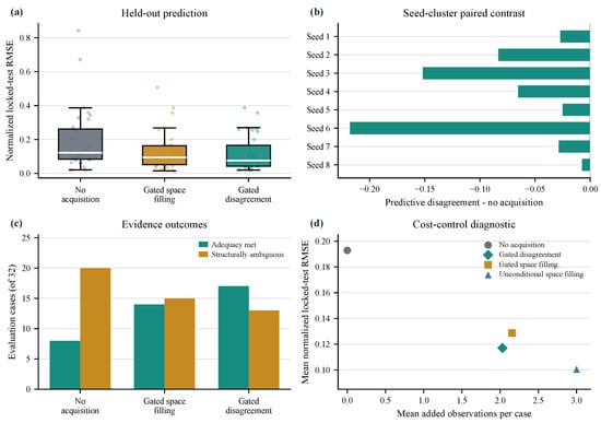
Mean normalized locked-test RMSE decreased from 0.193 without acquisition to 0.129 with conditional space filling and 0.117 with predictive disagreement (Table 2). Relative to the no-acquisition correction, this is a 39.3% reduction; the remaining error under predictive disagreement averaged 11.7% of the uncorrected baseline error. For the primary contrast, the paired mean difference was $-0.0758$, with a 95% seed-cluster bootstrap interval of $[-0.127,-0.032]$ and an add-one-corrected one-sided sign-flip p-value of 0.0078. The mean contrast favored acquisition in all eight seed clusters. The corresponding two-sided sensitivity analysis is reported in Supplementary Table S6.

Table 2. Seed-level out-of-sample evaluation across four response families and eight data seeds unused in development (32 paired cases). Error values are normalized locked-test RMSE.

Method	Mean	Median	Adequacy Met	Unresolved	Queries
No acquisition	0.19288	0.12149	8/32	20/32	0.000
Conditional space filling	0.12869	0.09363	14/32	15/32	2.156
Predictive disagreement	0.11706	0.07534	17/32	13/32	2.031

Note. Adequacy met is the number of cases satisfying ${\mathrm{RMSE}}_{\mathrm{locked}}\le \max \{3\sigma ,0.03\mathrm{sd}\left(y_{\mathrm{locked}}\right)\}$; it measures final prediction accuracy, not exact mechanism recovery. “Unresolved” reports the structural-ambiguity flag rather than a fourth status. Under the original physical checks, unresolved cases were provisional, all remaining cases were accepted, and none were rejected. Section S15 reports failures found with denser verification grids without changing these original assignments. “Queries” is the mean number of additional observations. Both acquisition policies used the same ambiguity gate defined before the evaluation. Predictive disagreement improved on no acquisition, whereas its difference from conditional space filling was not statistically significant.

Across no acquisition, conditional space filling, and predictive disagreement, adequacy was met in 8/32, 14/32, and 17/32 cases, respectively; the corresponding numbers retaining structural ambiguity were 20/32, 15/32, and 13/32. Both gated policies shared the same initial candidate pool and triggered in the same 27 cases. Thus, additional evidence improved reference-response adequacy and reduced structurally unresolved outcomes, although the casewise benefit was not uniform. The two gated policies were not statistically distinguished (mean difference $-0.0116$; cluster interval $[-0.0306,0.00554]$). Predictive disagreement was therefore competitive rather than demonstrably superior to conditional space filling.

The corrections selected by all three methods passed the original physical and complexity checks, and $q_0$ was absent from every final near-equivalent set. Under those checks, unresolved cases were provisional, the remainder accepted, and none rejected.

Performance varied by response family. The clearest gain occurred for permeability, where predictive-disagreement RMSE decreased from 0.0714 without acquisition to 0.0393 and all eight cases met the adequacy threshold. Conditional space filling slightly outperformed predictive disagreement for cyclic damage, and neither gated policy dominated across all response families. An independent check on denser, locally refined grids found that 94 of the 96 final corrected models satisfied the physical criteria. The other two, both from the same thermal-damage case, violated monotonicity near a domain boundary. Symbolic signs and adaptive interval bounds established the specified response constraints throughout the declared domains for 84 models, left ten undetermined, and confirmed the same two violations (Supplementary Section S15). These additional checks did not alter the fitted expressions or the original prediction comparisons.

3.3. Candidate Coverage and Identification Limits

Under predictive-disagreement acquisition, an LLM-generated proposal was selected as the final representative in 15 of 32 cases and appeared in 18 final near-equivalent sets. These attribution counts show that LLM proposals were competitive within the common evaluator and supplied candidates that survived deterministic screening, but they do not establish an accuracy advantage over PySR. The LLM itself had no role in coefficient fitting, verification, acquisition, or status assignment; valid outputs were treated as ordinary candidate expressions under the same deterministic evaluation.

A candidate-source ablation reevaluated the original candidates under the same evaluation procedure (Supplementary Section S13). With predictive-disagreement acquisition, mean normalized held-out RMSE was 0.107 for PySR alone, 0.179 for the LLM alone, and 0.117 for the original hybrid. The hybrid–PySR paired interval included zero; a common candidate cap of 12 did not establish a hybrid advantage either. The LLM supplied the reference expressions present in two initial candidate pools, although neither was retained or selected. It therefore contributed additional structures, while an incremental accuracy advantage over PySR was not established in this comparison. The ablation leaves the original primary comparison unchanged.

No representative exactly recovered the hidden expression. Normalizing parameter labels and commutative ordering did not change this result, and the exact structure appeared in only two of 32 initial candidate sets. The contrast between 17 cases meeting the response-adequacy threshold and zero exact recoveries shows why predictive adequacy and structural identification are reported separately.

3.4. Diagnostic Analyses

The first diagnostic used the candidate sets from the primary evaluation and inserted the reference expression where absent while leaving all original candidates and evaluation settings unchanged. All 32 sets then contained the exact structure, 14 retained it in the final near-equivalent set, and seven selected it as representative. Candidate coverage was therefore a major bottleneck, but coverage alone did not ensure identification under sparse noisy evidence. This oracle-insertion diagnostic distinguishes generation failure from downstream identifiability; it is not an estimate of prospective method performance.

The second diagnostic compared gated and unconditional space filling under the same maximum three-query budget (Figure 3d). Across the 32 cases, gating used 69 rather than 96 additional observations, a reduction of 28.1%, but increased mean normalized locked-test RMSE from 0.101 to 0.129. The gate therefore defines an explicit accuracy–observation-cost tradeoff rather than dominating full-budget acquisition. Detailed diagnostic results are given in Supplementary Section S11.

Figure 3. Predictive performance, ambiguity outcomes, and a supplementary cost analysis across the 32 evaluation cases. (a) Normalized locked-test RMSE. (b) Seed-cluster paired contrast for predictive disagreement relative to no acquisition. (c) Response adequacy and structural ambiguity. (d) Error–observation tradeoff under a fixed maximum query budget.

An auxiliary comparison of joint information with simpler acquisition rules, using fixed candidate sets, is reported in Supplementary Section S10; it is not treated as a separate methodological contribution.

3.5. Broader Coverage and a New Response Family

A separate 32-case evaluation used new data seeds and freshly generated candidates with observations distributed over the full declared domain. It also used fitting feedback during candidate generation and a rational-expression compilation rule, so it is not a single-factor ablation of observation coverage (Supplementary Section S12).

No case triggered acquisition: all three policies returned identical results, with mean normalized locked-test RMSE of 0.0204 and response adequacy in 31/32 cases. All selected corrections passed the physical checks used in that evaluation. The structural check identified a match to the reference expression family in 4/32 cases. This check concerns expression structure rather than exact coefficient values; failure to certify a match is not a proof of inequivalence. With no acquisitions, neither gated policy improved on the no-acquisition control. In one thermal-damage case, the retained candidates made similar predictions despite appreciable reference-response error. Agreement within a candidate set can thus suppress acquisition without ruling out a shared model discrepancy.

A separate test used average one-dimensional consolidation, a response family not used during development, with eight new data seeds (Supplementary Section S16). Predictive-disagreement acquisition reduced mean normalized error by 34.7% relative to no acquisition, from 0.826 to 0.539; conditional space filling achieved 0.547. Both used at most three additional observations per case and reduced the number of corrections exceeding the consolidation upper bound from eight to four. The response-adequacy threshold remained unmet, and a refined check found one monotonicity violation. The extension shows improved predictions beyond the development families, but further work is needed to meet the accuracy and physical constraints for this response. Full results are reported separately from the original primary analysis.

4. Geomechanical Evaluations

Section 3 provides the 32-case statistical evaluation. The geomechanical studies evaluate the method at three complementary levels: (i) controlled recovery and FLAC3D implementation of weak-plane laws; (ii) boundary-value propagation of a separately fixed correction; and (iii) grouped evaluation on published anisotropic-rock data. These studies test different aspects of the method, including when the available evidence does not justify accepting a correction; they do not form a single sequence of model transfer.

4.1. Controlled Constitutive Recovery and Solver Consistency

The first benchmark used the zero-dilation Mohr–Coulomb weak-plane relation in the FLAC3D ubiquitous-joint formulation [25],

$${\tau }_y=c-{\sigma }_n\tan \varphi ,$$

(13)

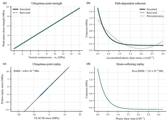
with compression taken as negative. Calibration and held-out paths varied weak-plane orientation, confinement, and loading history. The retained expression, ${\widehat{\tau }}_y/\mathrm{MPa}=1.2-0.5317({\sigma }_n/\mathrm{MPa})$, recovered the prescribed $c=1.2 \mathrm{MPa}$ and $\varphi ={28}^{\circ }$ values. Held-out RMSE decreased from approximately $1.43$ MPa for the intact-matrix baseline to numerical roundoff. Because an unconstrained polynomial containing the same linear term also fits this noise-free case, the benchmark verifies the correction representation and coefficient fitting rather than superiority over unconstrained regression.

The second benchmark introduced cumulative weak-plane plastic shear strain $\kappa$ and the prescribed cohesion law

$$c\left(\kappa \right)=c_r+(c_p-c_r)\exp \left(-{\displaystyle \frac{\kappa }{{\kappa }_c}}\right),$$

(14)

where $c_p=1.50 \mathrm{MPa}$, $c_r=0.35 \mathrm{MPa}$, and ${\kappa }_c=3.5\times {10}^{-4}$. The verifier required finite, non-negative, monotonically decreasing cohesion with an admissible residual value. The selected expression exactly recovered Equation (14), reducing held-out joint-stress RMSE from $0.453$ MPa for an ideally plastic weak plane to numerical roundoff. An unconstrained quadratic reached $0.103$ MPa but predicted increasing cohesion within the verification interval. The comparison shows why predictive error alone is insufficient for selecting a state law. Machine-precision recovery is expected here because the data are noise-free and the reference family is available.

The two fixed updates were then reproduced independently in FLAC3D 7.0. Across seven ubiquitous-joint paths and four strain-softening paths, stress RMSE between the standalone and FLAC3D calculations did not exceed $7.61\times {10}^{-6}$ MPa; yield onset and internal-state evolution also agreed to numerical tolerance (Table 3). This verifies implementation consistency along the prescribed loading paths. Complete path definitions and solver-transfer details are reported in Supplementary Section S8.

Table 3. Constitutive-law recovery and FLAC3D material-point implementation verification.

Case	Evaluation	Result	Interpretation
Linear weak-plane strength	Held-out RMSE, baseline → correction (MPa)	$1.430\to$ roundoff	Prescribed linear relation recovered
Cohesion softening	Held-out RMSE, baseline → correction (MPa)	$0.453\to$ roundoff	Prescribed exponential state law recovered
Unconstrained polynomial	Held-out joint-stress RMSE (MPa)	0.103	Lower error than baseline, but one monotonicity violation
Ubiquitous-joint replay	Stress RMSE over seven paths (MPa)	$4.00\times {10}^{-6}$	Standalone and FLAC3D calculations agree
Strain-softening replay	Stress RMSE over four paths (MPa)	$7.61\times {10}^{-6}$	State updates and softening tables agree

Figure 4 compares the recovered constitutive laws and the material-point implementations.

Figure 4. Constitutive-law recovery and solver implementation. (a) Prescribed and recovered ubiquitous-joint strength. (b) Prescribed, recovered, and polynomial cohesion-softening laws. (c) Ubiquitous-joint and (d) strain-softening responses along fixed FLAC3D single-zone loading paths. In (c), points compare stress components from the two implementations and the dashed line denotes equality. In (d), gray solid lines denote FLAC3D cohesion histories and teal dashed lines denote the standalone replay.

4.2. Boundary-Value Propagation of a Fixed Correction

The boundary-value test used a two-dimensional plane-strain model of an idealized hydropower cavern, 34 m wide and $88.7$ m high, excavated in six stages. The three laws were first compared on the same body-fitted mesh, with identical support, far-field loading, and bedding/loading orientation; complete settings are given in Supplementary Table S7. Supplementary Figure S1 shows the geometry, mesh, support, displacement, stress, and yielded zones for this case after the sixth excavation stage.

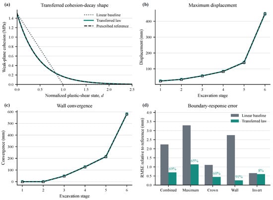
Normalized weak-plane plastic shear was $d=\kappa /(3.5\times {10}^{-4})$. Before the cavern study, the functional form and normalized decay coefficient of $a_0\exp (-a_{1}d)$ had been fixed in an independent source benchmark. Only its dimensional amplitude was rescaled by the prescribed peak-cohesion ratio $1.5/4.0$. The compared laws were

$$\begin{array}{cc}\hfill c_{\mathrm{base}}\left(d\right)& =1.5\max (1-d,0),\hfill \\ \hfill c_{\mathrm{disc}}\left(d\right)& =1.498\exp (-2.192d),\hfill \\ \hfill c_{\mathrm{ref}}\left(d\right)& =1.5\exp (-2.2d),\hfill \end{array}$$

(15)

in MPa. The source reference was unavailable during candidate generation and fitting. A reference-only load qualification was completed before the transferred law was evaluated; the retained case satisfied the minimum-signal criterion fixed in advance. Supplementary Tables S7 and S8 document the numerical threshold, qualification, and transfer.

All excavation stages converged, and all three laws activated weak-plane plasticity. Relative to the prescribed reference, joint RMSE over maximum displacement, crown displacement, wall convergence, and invert displacement decreased from $2.24$ mm for the linear baseline to $0.694$ mm for the transferred law, a 69.0% reduction. Stagewise joint RMSE decreased at every excavation stage, but the improvement was response-dependent: wall-convergence RMSE decreased by 90.6%, whereas invert-displacement RMSE decreased by only 8.5%. Table 4 reports the complete response-specific results. Because the correction modifies the cohesion table used by the constitutive update, FLAC3D updates stresses and re-establishes equilibrium after every excavation stage rather than post-processing a fixed response.

Table 4. FLAC3D propagation of a normalized cohesion-decay shape transferred from the source benchmark.

Quantity	Linear Baseline	Transferred Law	Interpretation
Multi-response RMSE (mm)	2.237	0.694	69.0% reduction; prespecified criterion met (≥50%)
Maximum absolute response error (mm)	7.284	2.763	Reduced over six stages
Maximum-displacement RMSE (mm)	3.287	1.140	65.3% reduction
Crown-displacement RMSE (mm)	1.106	0.444	59.8% reduction
Wall-convergence RMSE (mm)	2.749	0.259	90.6% reduction
Invert-displacement RMSE (mm)	0.656	0.601	8.5% reduction
Maximum plastic-zone count	381	390	Reference: 390; all models activated plasticity
Converged excavation stages	6/6	6/6	Average force ratio $\le {10}^{-5}$

Note. Errors are measured against the prescribed exponential reference on the original 1392-zone mesh. The baseline–reference multi-response difference was 1.33%, above the prespecified minimum signal of 1%. The two-mesh comparison is in Supplementary Table S15. Neither calculation is a field validation.

Figure 5 compares the three cohesion laws and their stage-wise cavern responses.

Figure 5. Constitutive propagation through staged cavern excavation. (a) Linear baseline, transferred cohesion-decay law, and prescribed reference. (b) Maximum displacement and (c) wall convergence over six stages. (d) RMSE relative to the reference; percentages denote reductions from the baseline. In (b,c), gray dotted lines with circles denote the linear baseline, teal solid lines with squares denote the transferred law, and dark dashed lines with triangles denote the prescribed reference.

An additional calculation repeated all three fixed laws on a 3132-zone mesh, retaining the loading, material parameters, support sequence, and convergence criterion. Combined RMSE relative to the reference solution on that mesh decreased from 47.2 to $14.5$ mm, a 69.3% reduction, compared with 69.0% on the original mesh. Absolute responses remained strongly mesh-sensitive (Supplementary Section S17 and Table S15). The relative improvement therefore persisted on both meshes, but this does not establish mesh convergence or mesh-objective softening. The study remains a numerical test at one load and orientation, separate from the preceding cohesion-recovery benchmark and from validation for engineering use.

4.3. Grouped Evaluation on Published Anisotropic-Rock Data

In anisotropic rock, Brazilian-disc interpretation depends on the stress field and layer orientation [26,27,28]. Crack initiation, failure mode, and the relation between nominal and material tensile strength can also vary with transverse-isotropy orientation [29,30].

Four small datasets test whether the framework withholds corrections that do not improve grouped validation. Dinh reported Brazilian-test measurements and numerical central-stress predictions for Leubsdorfer gneiss (Le.Gs) and Mayen Mosel slate (My.Sc) over bedding/loading orientation grids [31,32]; Ma et al. compiled measured and predicted Brazilian tensile strengths, from which Longmaxi shale and Jixi coal were used [33]. Complete angle groups were withheld. For the Dinh datasets, the reported score is the average of leave-one-$\beta$ and leave-one-$\psi$ RMSE; for the Ma datasets, it is leave-one-$\beta$ RMSE. The results assess interpolation across withheld orientations within each publication, not cross-material generalization.

Corrections were accepted for My.Sc and Longmaxi shale, reducing Group-CV RMSE by 30.5% and 36.7%, respectively. Le.Gs and Jixi coal instead showed small error increases and remained provisional (Table 5). The published-data evaluation therefore records both successful corrections and cases in which the available evidence did not support acceptance.

Table 5. Grouped validation on literature-derived anisotropic-rock datasets.

Dataset	Baseline	Corrected	RMSE Change	Outcome
Dinh Le.Gs	2.3771	2.4542	$+3.2\%$	Provisional
Dinh My.Sc	2.1954	1.5255	$-30.5\%$	Accepted
Ma Longmaxi shale	0.2131	0.1350	$-36.7\%$	Accepted
Ma Jixi coal	0.0214	0.0223	$+4.2\%$	Provisional

Note. RMSE is in MPa; a negative change indicates improvement. Dinh values average leave-one-$\beta$ and leave-one-$\psi$ errors; Ma values use leave-one-$\beta$. “Provisional” denotes a correction that failed the improvement criterion and was therefore not accepted. These are grouped-validation results within each dataset, not independent cross-study tests.

The accepted residual expressions were

$$\begin{array}{cc}\hfill {\widehat{r}}_{\mathrm{My}.\mathrm{Sc}}=& 0.0111-2.096\sin \beta +3.717\sin \psi -11.15m_{\psi }^2,\hfill \end{array}$$

(16)

$$\begin{array}{cc}\hfill {\widehat{r}}_{\mathrm{Longmaxi}}=& 0.00440+22.49{\displaystyle \frac{m_{\beta }^2}{1+3m_{\beta }^2}}-2.945\sin \left(2\beta \right),\hfill \end{array}$$

(17)

where $m_{\alpha }=\left|\sin \alpha \cos \alpha \right|\in [0,1/2]$ and coefficients are in MPa. Source angles are converted from degrees to radians before trigonometric evaluation. The bounded angular terms represent smooth orientation trends and variation at intermediate orientations, but the small grouped datasets do not identify a unique crack-initiation mechanism. Supplementary Figure S2 shows the grouped-error comparison and accepted correction surfaces.

5. Discussion

5.1. What Conditional Acquisition Contributes

The primary evaluation supports obtaining additional evidence when sparse initial observations leave admissible corrections unresolved. The three methods shared candidate sets, coefficient fitting, and verification, so the paired comparison isolates acquisition rather than a larger search budget. Predictive disagreement gave the lowest mean error, but its advantage over conditional space filling was not statistically established. The practical result is therefore support for conditional evidence collection, not a universal ranking of sampling policies.

The gate controls the number of additional observations and the associated accuracy–observation-cost tradeoff. Conditional space filling saved 27 of 96 possible observations relative to unconditional acquisition, with a mean normalized error increase of 0.0279. This tradeoff is relevant when laboratory tests or numerical evaluations are costly. The present threshold was fixed before evaluation; selecting a different tradeoff would require new validation data rather than adjustment to the reported locked-test outcomes.

The threshold also affects the meaning of a resolved outcome. In the sensitivity analysis, increasing the threshold from $\sigma$ to $4\sigma$ reduced predictive-disagreement observations from 73 to 55, while mean normalized error increased from 0.115 to 0.133. The number classified as structurally ambiguous decreased from 18 to seven (Supplementary Section S14). Fewer unresolved cases at a higher threshold therefore need not imply more accurate corrections. The original $2\sigma$ setting was retained; it is an operational tolerance, not a calibrated probability of correctness.

The full-domain evaluation illustrates why candidate agreement must be distinguished from accuracy. All acquisition policies returned the same results because no gate triggered, and most cases met the response-adequacy criterion. However, one thermal-damage case retained substantial error while its candidates agreed. The gate can detect ambiguity only among the expressions available to it; agreement does not exclude a shared model discrepancy.

5.2. Interpreting an Explicit Correction

An explicit equation makes a modification inspectable, but does not make its structure uniquely identified. No final representative exactly recovered the hidden expression in the primary evaluation, even though prediction improved. The reference structure was present in only two of 32 initial pools. Inserting it into all pools in the oracle diagnostic led to 14 retained exact candidates and only seven selected representatives. Both candidate coverage and discrimination using limited observations therefore constrained recovery.

The LLM provided an additional source of candidate structures, including the reference expressions present in two initial pools. The source ablation did not establish an incremental accuracy advantage over PySR for these cases. Mean generation times recorded in the original runs were about 205 s per case for the LLM and 5 s for PySR, before fitting and verification. These descriptive timings were not obtained under matched computational budgets and do not establish a general cost–benefit ranking. Candidate-source choice can therefore reflect the application and available resources; the evaluation and acquisition procedure supports both PySR-only and hybrid generation.

5.3. Implications for Rock-Mechanics Applications

The controlled constitutive tests show why numerical accuracy and mechanical admissibility must be considered together. An unconstrained quadratic reduced the softening-benchmark error but predicted increasing cohesion within the verification interval. The retained exponential law satisfied monotonicity and the residual-cohesion requirement. Its exact recovery is expected under noise-free data and an available reference family; the FLAC3D comparisons then test implementation consistency along prescribed loading paths.

The cavern study asks a different question: can a correction shape selected independently improve a boundary-value response after constitutive updates and equilibrium solution? The functional form and normalized decay coefficient were fixed before the calculation, while the amplitude was rescaled by the prescribed peak-cohesion ratio. Combined response error decreased by 69.0% on the original mesh and 69.3% on the finer mesh. These similar relative reductions must be interpreted alongside the substantial changes in absolute responses under refinement. Local softening remains unregularized, and further assessment across loading conditions is needed before engineering application.

The literature datasets illustrate use without acquiring new observations. Two corrections improved complete-angle-group validation, whereas two remained provisional. The accepted bounded angular terms represent orientation trends, but the small within-publication datasets do not identify unique crack mechanisms or establish cross-material transfer. For an engineering assessment, the useful output is therefore an explicit correction accompanied by its validation domain and unresolved alternatives, not an unqualified replacement for the original model.

In practice, updating starts from a calibrated baseline and observations at accessible loading conditions, orientations, or monitoring locations. The query set must respect those constraints: a fixed sensor installation cannot supply arbitrary measurements. An additional query may instead correspond to a laboratory test, a controlled loading stage, or a numerical evaluation. Gating is useful when such observations are costly and the associated accuracy tradeoff is acceptable. When observations are inexpensive, or the engineering decision requires tighter error control, fixed-budget acquisition may be preferable. If further measurements are unavailable, unresolved alternatives remain provisional. The noise scale should come from repeated measurements, instrument calibration, or an independent error model; using all baseline residual error as measurement noise would absorb model discrepancy and can suppress acquisition.

5.4. Limitations and Further Evaluation

The primary study used new data realizations from four families known during development; the consolidation extension provides an initial test beyond those families. Inference for the primary comparison is based on eight seed clusters. The physical-check results in Section 3 and Supplementary Section S15 distinguish constraints established over continuous domains from properties tested only at finite points. The two corrections with confirmed monotonicity violations do not satisfy the requirements for use. The full-domain study changed candidate processing as well as observation coverage and cannot isolate the effect of either change alone.

The 32-case study concerns output-level corrections. Component replacement is supported by the representation and tested in controlled weak-plane examples, but the experiments do not demonstrate open-ended localization of an unknown constitutive defect. Independent laboratory or field measurements are needed before engineering deployment; localized softening also requires regularization and discretization assessment. Further method evaluation should distinguish when additional observations resolve competing expressions from when the expression set itself must be expanded.

6. Conclusions

An evidence-gated symbolic correction framework was developed for geomechanical problems with an existing baseline and limited observations. It separates candidate generation from numerical fitting, grouped validation, physical verification, and acceptance. Additional observations are requested when retained admissible expressions disagree; an unsupported correction remains provisional rather than being selected solely for its fitting error.

Across the 32 primary evaluation cases, predictive-disagreement acquisition reduced mean normalized locked-test RMSE from 0.193 to 0.117 relative to no acquisition. Its advantage over conditional space filling was not statistically established. The fixed-budget control showed that gating saved 28.1% of space-filling observations at an accuracy cost, demonstrating an explicit error–observation tradeoff.

Controlled weak-plane tests verified constitutive-law recovery and FLAC3D material-point implementation. A separate cavern calculation provided a numerical demonstration: multi-response RMSE against a prescribed reference decreased from 2.24 to $0.694$ mm. Relative error reductions were similar on the original and finer meshes (69.0% and 69.3%), although absolute responses remained mesh-sensitive. Published rock data supported two corrections and left two provisional. These results address complementary levels of model evaluation.

The consolidation extension also showed prediction improvement beyond the development families, with a 34.7% reduction in mean normalized error relative to no acquisition. Predictive improvement, exact structural recovery, and physical admissibility remain distinct outcomes. The practical contribution is a transparent procedure for assessing explicit corrections and directing additional observations while retaining unresolved alternatives when the evidence is insufficient.

References

- Kennedy, M.C.; O’Hagan, A. Bayesian Calibration of Computer Models. J. R. Stat. Soc. Ser. B Stat. Methodol. 2001, 63, 425–464. [Google Scholar] [CrossRef] [Scilit]
- Bock, F.E.; Keller, S.; Huber, N.; Klusemann, B. Hybrid Modelling by Machine Learning Corrections of Analytical Model Predictions towards High-Fidelity Simulation Solutions. Materials 2021, 14, 1883. [Google Scholar] [CrossRef] [Scilit] [PubMed]
- Karniadakis, G.E.; Kevrekidis, I.G.; Lu, L.; Perdikaris, P.; Wang, S.; Yang, L. Physics-Informed Machine Learning. Nat. Rev. Phys. 2021, 3, 422–440. [Google Scholar] [CrossRef] [Scilit]
- Masi, F.; Stefanou, I.; Vannucci, P.; Maffi-Berthier, V. Thermodynamics-Based Artificial Neural Networks for Constitutive Modeling. J. Mech. Phys. Solids 2021, 147, 104277. [Google Scholar] [CrossRef] [Scilit]
- Linka, K.; Hillgärtner, M.; Abdolazizi, K.P.; Aydin, R.C.; Itskov, M.; Cyron, C.J. Constitutive Artificial Neural Networks: A Fast and General Approach to Predictive Data-Driven Constitutive Modeling by Deep Learning. J. Comput. Phys. 2021, 429, 110010. [Google Scholar] [CrossRef] [Scilit]
- Haghighat, E.; Raissi, M.; Moure, A.; Gomez, H.; Juanes, R. A Physics-Informed Deep Learning Framework for Inversion and Surrogate Modeling in Solid Mechanics. Comput. Methods Appl. Mech. Eng. 2021, 379, 113741. [Google Scholar] [CrossRef] [Scilit]
- Schmidt, M.; Lipson, H. Distilling Free-Form Natural Laws from Experimental Data. Science 2009, 324, 81–85. [Google Scholar] [CrossRef] [Scilit] [PubMed]
- Brunton, S.L.; Proctor, J.L.; Kutz, J.N. Discovering Governing Equations from Data by Sparse Identification of Nonlinear Dynamical Systems. Proc. Natl. Acad. Sci. USA 2016, 113, 3932–3937. [Google Scholar] [CrossRef] [Scilit] [PubMed]
- Udrescu, S.M.; Tegmark, M. AI Feynman: A Physics-Inspired Method for Symbolic Regression. Sci. Adv. 2020, 6, eaay2631. [Google Scholar] [CrossRef] [Scilit] [PubMed]
- Petersen, B.K.; Landajuela, M.; Mundhenk, T.N.; Santiago, C.P.; Kim, S.K.; Kim, J.T. Deep Symbolic Regression: Recovering Mathematical Expressions from Data via Risk-Seeking Policy Gradients. In Proceedings of the International Conference on Learning Representations, Virtual, 3–7 May 2021. [Google Scholar]
- Kamienny, P.A.; d’Ascoli, S.; Lample, G.; Charton, F. End-to-End Symbolic Regression with Transformers. In Advances in Neural Information Processing Systems; Neural Information Processing Systems Foundation, Inc.: San Diego, CA, USA, 2022; Volume 35, pp. 10269–10281. [Google Scholar]
- Zhang, P.; Yin, Z.Y.; Sheil, B. Interpretable Data-Driven Constitutive Modelling of Soils with Sparse Data. Comput. Geotech. 2023, 160, 105511. [Google Scholar] [CrossRef] [Scilit]
- Guayacán-Carrillo, L.M.; Sulem, J. Symbolic Regression Based Prediction of Anisotropic Closure in Deep Tunnels. Comput. Geotech. 2024, 171, 106355. [Google Scholar] [CrossRef] [Scilit]
- Foroughi Boroujeni, F.; Faramarzi, A.; Cha, W.; Ghiassi, B.; Rahimzadeh, F. A Physics-Informed Evolutionary Regression Framework for Constitutive Modelling of Sand. Comput. Geotech. 2026, 197, 108179. [Google Scholar] [CrossRef] [Scilit]
- Tao, L.; Zhang, R.; Zou, Y.; Wang, Y. Geomechanics-Motivated Discovery of Three-Dimensional Coupled Governing Equations via Physics-Informed Symbolic Genetic Algorithms. Comput. Geotech. 2026, 197, 108187. [Google Scholar] [CrossRef] [Scilit]
- La Cava, W.; Orzechowski, P.; Burlacu, B.; de França, F.O.; Virgolin, M.; Jin, Y.; Kommenda, M.; Moore, J.H. Contemporary Symbolic Regression Methods and Their Relative Performance. In Proceedings of the Neural Information Processing Systems Track on Datasets and Benchmarks; Neural Information Processing Systems Foundation, Inc.: San Diego, CA, USA, 2021; Volume 1. [Google Scholar]
- Cranmer, M. Interpretable Machine Learning for Science with PySR and SymbolicRegression.jl. arXiv 2023, arXiv:2305.01582. [Google Scholar] [CrossRef] [Scilit]
- Virgolin, M.; Pissis, S.P. Symbolic Regression Is NP-Hard. arXiv 2022, arXiv:2207.01018. [Google Scholar]
- Atkinson, A.C.; Fedorov, V.V. The Design of Experiments for Discriminating between Two Rival Models. Biometrika 1975, 62, 57–70. [Google Scholar] [CrossRef]
- Chaloner, K.; Verdinelli, I. Bayesian Experimental Design: A Review. Stat. Sci. 1995, 10, 273–304. [Google Scholar] [CrossRef] [Scilit]
- Houlsby, N.; Huszár, F.; Ghahramani, Z.; Lengyel, M. Bayesian Active Learning for Classification and Preference Learning. arXiv 2011, arXiv:1112.5745. [Google Scholar] [CrossRef] [Scilit]
- Merler, M.; Haitsiukevich, K.; Dainese, N.; Marttinen, P. In-Context Symbolic Regression: Leveraging Large Language Models for Function Discovery. In Proceedings of the 62nd Annual Meeting of the Association for Computational Linguistics (Volume 4: Student Research Workshop); Association for Computational Linguistics: Bangkok, Thailand, 2024; pp. 427–444. [Google Scholar] [CrossRef] [Scilit]
- Shojaee, P.; Meidani, K.; Gupta, S.; Barati Farimani, A.; Reddy, C.K. LLM-SR: Scientific Equation Discovery via Programming with Large Language Models. In Proceedings of the International Conference on Learning Representations, Singapore, 24–28 April 2025. [Google Scholar]
- Shojaee, P.; Nguyen, N.H.; Meidani, K.; Barati Farimani, A.; Doan, K.D.; Reddy, C.K. LLM-SRBench: A New Benchmark for Scientific Equation Discovery with Large Language Models. In Proceedings of the 42nd International Conference on Machine Learning, Vancouver, BC, Canada, 13–19 July 2025; Proceedings of Machine Learning Research: San Diego, CA, USA, 2025; Volume 267, pp. 55325–55359. [Google Scholar]
- Itasca Consulting Group. FLAC3D 7.0 Documentation: Ubiquitous-Joint Model, Version 7.0; Itasca Consulting Group, Inc.: Minneapolis, MN, USA, 2024. [Google Scholar]
- Claesson, J.; Bohloli, B. Brazilian Test: Stress Field and Tensile Strength of Anisotropic Rocks Using an Analytical Solution. Int. J. Rock Mech. Min. Sci. 2002, 39, 991–1004. [Google Scholar] [CrossRef] [Scilit]
- Tavallali, A.; Vervoort, A. Effect of Layer Orientation on the Failure of Layered Sandstone under Brazilian Test Conditions. Int. J. Rock Mech. Min. Sci. 2010, 47, 313–322. [Google Scholar] [CrossRef] [Scilit]
- Li, D.; Wong, L.N.Y. The Brazilian Disc Test for Rock Mechanics Applications: Review and New Insights. Rock Mech. Rock Eng. 2013, 46, 269–287. [Google Scholar] [CrossRef] [Scilit]
- Vervoort, A.; Min, K.B.; Konietzky, H.; Cho, J.W.; Debecker, B.; Dinh, Q.D.; Frühwirt, T.; Tavallali, A. Failure of Transversely Isotropic Rock under Brazilian Test Conditions. Int. J. Rock Mech. Min. Sci. 2014, 70, 343–352. [Google Scholar] [CrossRef] [Scilit]
- Aliabadian, Z.; Zhao, G.F.; Russell, A.R. Failure, Crack Initiation and the Tensile Strength of Transversely Isotropic Rock Using the Brazilian Test. Int. J. Rock Mech. Min. Sci. 2019, 122, 104073. [Google Scholar] [CrossRef] [Scilit]
- Dinh, Q.D. Brazilian Test on Anisotropic Rocks: Laboratory Experiment, Numerical Simulation and Interpretation. Ph.D. Thesis, TU Bergakademie Freiberg, Freiberg, Germany, 2011. [Google Scholar]
- Dinh, Q.D.; Konietzky, H.; Herbst, M. Brazilian Tensile Strength Tests on Some Anisotropic Rocks. Int. J. Rock Mech. Min. Sci. 2013, 58, 1–7. [Google Scholar] [CrossRef] [Scilit]
- Ma, T.; Peng, N.; Zhu, Z.; Zhang, Q.; Yang, C.; Zhao, J. Brazilian Tensile Strength of Anisotropic Rocks: Review and New Insights. Energies 2018, 11, 304. [Google Scholar] [CrossRef] [Scilit]
Disclaimer/Publisher’s Note: The statements, opinions and data contained in all publications are solely those of the individual author(s) and contributor(s) and not of MDPI and/or the editor(s). MDPI and/or the editor(s) disclaim responsibility for any injury to people or property resulting from any ideas, methods, instructions or products referred to in the content. |
© 2026 by the authors. Licensee MDPI, Basel, Switzerland. This article is an open access article distributed under the terms and conditions of the Creative Commons Attribution (CC BY) license.