Supervised Contrastive Learning with Magnitude-Based Pruning for Arabic Traffic Sign Recognition

Abstract

The rapid development of smart cities in the Arab region has accelerated the growth of Intelligent Transportation Systems (ITS), in which automatic traffic sign recognition plays an essential role in supporting road safety and intelligent vehicle applications. However, recognising Arabic traffic signs remains challenging due to the complexity of Arabic script. In addition, the limited computational and memory resources of automotive hardware highlight the need for compact and accurate recognition models. To address these challenges, this study proposes a framework that integrates supervised contrastive learning with magnitude-based pruning. Supervised contrastive learning enhances discriminative feature representations, while magnitude-based pruning introduces sparsity by removing low-magnitude weights. Four main configurations, namely the end-to-end ResNet50V2 baseline, the pruned baseline, the two-stage SCL model and the pruned SCL model, were evaluated across ten random seeds. The SCL model achieved an accuracy of 98.90 ± 0.50%, significantly higher than that of the end-to-end baseline (98.47 ± 0.28%; $p=0.016$, unadjusted). Magnitude-based pruning achieved 80% sparsity in the Dense-layer weights while preserving classification performance, with the pruned baseline and pruned SCL models achieving accuracies of 99.07% and 99.00%, respectively. Furthermore, pruning reduced the gzip-compressed model size by approximately 3.4%, whereas int8 quantisation reduced the model size from 99.35 to 25.48 MB. These findings indicate that the integration of SCL with magnitude-based pruning can maintain high recognition accuracy while introducing weight sparsity, highlighting its potential for future applications in ITS.

1. Introduction

Image recognition is an important area of computer vision that enables machines to recognise and classify visual information based on features and patterns extracted from images. There are numerous applications of image recognition across various fields, including medicine, transport, archaeology, and environmental science. In medicine, image recognition supports disease diagnosis through skin lesion and melanoma analysis [1,2,3], blood cell identification [4], human peripheral blood leukocyte classification [5,6,7], and online identity authentication of blood smears [8]. Within transport, it is applied to traffic sign recognition [9,10,11], ship type classification [12], and driving behaviour classification [13]. Other applications of image recognition include fossil [14] and artefact classification [15], lithic microwear classification [16], archaeological site identification [17], and cultural heritage documentation in archaeology and palaeontology [18]. Additionally, in environmental science, it is used for land-use and land-cover classification [19], forest disturbance detection [20], plant disease detection and classification [21], and water-quality assessment [22]. The importance of image recognition in these areas lies in its ability to reduce manual effort and improve the accuracy and efficiency of visual data analysis. Among the various applications of image recognition, traffic sign recognition is particularly important for road safety, as accurate and timely recognition of traffic signs is a key requirement for advanced driver-assistance systems (ADAS) and autonomous vehicles.

Traffic sign recognition is also an essential component of Intelligent Transportation Systems (ITS), which are used in smart cities to manage urban traffic and address road safety issues. These systems employ technologies such as machine learning algorithms, sensor networks, and real-time data analytics to monitor, evaluate, and optimise multimodal transportation systems [23,24,25]. Within ITS, automated traffic sign recognition (ATSR) contributes to applications such as autonomous driving and smart traffic management infrastructure [26,27,28,29]. The development of ITS has become particularly relevant in the Middle East, where rapid urbanisation has made the region one of the most urbanised areas in the developing world, with over 60% of the population living in urban centres [30]. This rapid urban growth has increased the need for advanced traffic management systems to address complex transportation challenges.

Recent advances in deep learning models have significantly impacted computer vision tasks such as traffic sign recognition, with notable progress having been made for European [31,32,33,34], North American [35,36], and East Asian traffic sign recognition problems [37,38,39]. However, Arabic traffic sign (ArTS) recognition has received comparatively less research attention despite the growing interest in autonomous vehicles and ITS infrastructure across Arabic-speaking regions.

Arabic traffic signs present distinct recognition challenges that differentiate them from Western signage systems. The morphological complexity of Arabic script, characterised by right-to-left text orientation and context-dependent character variations, presents significant challenges. Additionally, the integration of Indian numerals introduces unique recognition difficulties [40,41]. Furthermore, subtle typographical differences, especially the presence or absence of diacritical marks (tashkeel), can significantly change meaning, requiring recognition systems to achieve high precision. The design paradigms and visual characteristics of Middle Eastern signage differ from Western standards, which may limit the effectiveness of directly applying recognition models trained on Western traffic sign datasets and motivate domain-specific adaptation.

Although deep learning-based computer vision systems have achieved remarkable success across various recognition tasks, their application to domain-specific recognition problems remains challenging [42]. Many existing approaches rely on conventional transfer learning techniques optimised using the widely adopted cross-entropy (CE) objective function [43,44]. However, these approaches may face difficulties under challenging visual conditions, limited training data, or the domain-specific characteristics encountered in Arabic traffic sign recognition [45]. These difficulties become more pronounced when recognition must be performed reliably and in real time.

Attention mechanisms have been widely applied in deep learning to improve feature extraction by enabling neural networks to focus on informative features while reducing the influence of irrelevant information [46]. In CNN-based image recognition, attention mechanisms include channel attention, spatial attention, and self-attention. Channel attention assigns different weights to feature channels according to their importance [47], whereas spatial attention emphasises relevant regions within an image and helps reduce background interference [48]. Self-attention captures relationships between different image regions, enabling models to learn long-range dependencies and contextual information [49]. Attention mechanisms have also been incorporated into residual architectures through residual attention networks [50] and mixed residual attention networks for medical image super-resolution [51]. They have been applied to graph-structured data through graph attention networks [52], for example, in joint event extraction using dynamic attention matching [53]. These mechanisms have been used in various tasks, including image classification [46,50], medical image analysis [54], remote sensing [49], single-shot fringe projection profilometry using a multi-attention fringe restoration network [55], and knowledge tracing using a cognitive fluctuations enhanced attention network [56]. In traffic sign recognition, attention-based approaches have been used to highlight important visual features and improve recognition performance [57,58]. They may also be relevant to Arabic traffic sign recognition, where distinguishing visually similar signs requires recognising fine details, including Arabic text, numerals, and diacritical marks. While attention mechanisms enhance feature representations by emphasising relevant visual information, supervised contrastive learning offers a complementary approach to improving feature discrimination through the training objective.

Supervised contrastive learning (SCL) has emerged as a promising alternative to conventional cross-entropy optimisation by explicitly learning discriminative feature embeddings through the optimisation of the embedding space [59,60]. Unlike traditional methods that optimise individual sample classification through direct class prediction, SCL learns representations through relational optimisation, wherein intra-class samples are encouraged to form compact clusters while inter-class samples are pushed further apart in the embedding space [61]. These properties make SCL a promising approach for Arabic traffic sign recognition, where visually similar classes need to be distinguished accurately.

However, implementing complex deep learning models in practical ITS applications presents challenges related to computational and resource limitations [62]. Automotive hardware platforms place more stringent requirements on model size, inference latency, and power consumption, necessitating efficient network compression methods that maintain high recognition accuracy while meeting deployment constraints [63]. Model pruning has emerged as an effective compression technique that systematically identifies and removes less important network connections while preserving critical feature representations. During the pruning process, connections with weights below a predetermined threshold are eliminated, creating a sparse network architecture [64]. The pruned model is subsequently fine-tuned to compensate for any accuracy degradation resulting from weight removal. Unstructured pruning reduces the number of non-zero parameters, although improvements in model storage and inference speed depend on how the sparse model is stored and executed. The challenge lies in developing frameworks that can achieve the accuracy-efficiency trade-offs necessary for potential deployment in resource-constrained ITS applications. The main contributions of this study are as follows:

• We develop a ResNet50V2-based transfer learning framework for Arabic traffic sign recognition to compare end-to-end baseline and supervised contrastive learning models, both with and without pruning.
• We investigate the integration of supervised contrastive learning with magnitude-based Dense-layer pruning to evaluate their effects on recognition accuracy and model sparsity.
• We conduct a controlled multi-seed evaluation of end-to-end, supervised contrastive, and cross-entropy two-stage training strategies, alongside model compression and computational efficiency, to assess their potential for resource-constrained ITS applications.

The remainder of this paper is structured as follows. Section 2 provides a review of the relevant literature on traffic sign recognition. Section 3 presents the proposed framework, encompassing transfer learning, supervised contrastive learning, and magnitude-based pruning. Section 4 details the dataset, evaluation metrics, implementation settings, and experimental findings. Finally, Section 5 summarises the main conclusions and discusses directions for future research.

2. Literature Review

Traffic Sign Recognition (TSR) has made significant progress through deep learning methods; however, there are still major challenges in recognizing non-Latin scripts, especially Arabic traffic signs. This section offers a thorough review of the latest TSR techniques and highlights the key research gaps that this study aims to address.

In [40], the authors proposed a modified ResNet architecture for Arabic traffic sign classification using the ArTS dataset. They adopt a strategy for the repeated stacking of ResNet blocks to form increasingly deeper networks that allow control over the network complexity. This repeated structure brings the optimized ResNet V1 to 96.14% test accuracy, and the ResNet V2 to 94.40% test accuracy, both higher than their standard counterparts.

Khalifa et al. [65] introduced a Lightweight and Efficient Convolutional Neural Network (LE-CNN) for Arabic traffic sign recognition that achieves a test accuracy of 96.5% on the ArTS and ATTICA datasets. Their LE-CNN architecture comprises three convolutional blocks (each followed by rectified linear unit (ReLU) activation and max-pooling), three dropout layers, a flattening stage, and a final softmax output. During training, 32 × 32 red, green and blue (RGB) images are augmented, and hyperparameters are set to a learning rate of 0.001 with the Adam optimiser, 32 sample mini-batches, and 100 epochs. Performance is validated via 5-fold stratified cross-validation to preserve class balance.

A comprehensive evaluation of six deep-learning architectures (MobileNetV2, EfficientNetB0, DenseNet121, ResNet50, InceptionV3, and NASNetLarge) was carried out on the ArTS traffic sign dataset [41]. After extensive preprocessing (scaling, random rotations, flips, translations, and normalisation), each model was trained using a 5-fold cross-validation scheme (10 epochs per fold) with an Adam optimiser (learning rate = 0.001), a batch size of 32, and either ReLU or Swish activations. DenseNet121 achieved the highest performance, achieving 98.52% validation accuracy and 96.54% test accuracy. The authors recommend transfer learning from more diverse datasets, adding new sign categories, and applying real-time data augmentation to enhance recognition of rare traffic signs.

Wang et al. [33] address the challenge of reducing computational costs in large-scale traffic sign recognition systems through a novel pruning framework. Their approach combines: (1) image preprocessing (normalisation, enhancement), (2) Vision Transformer (ViT) pre-training, and (3) model optimization via joint loss minimization (LLE + ADMM-based terms), followed by (4) filter pruning using JS-divergence to evaluate and remove redundant filters. Evaluated on the BelgiumTS and GTSRB datasets, their SJ-LLE method outperforms existing pruning techniques (ASFP, HYDRA, Filter, FPGM), achieving a 70% pruning ratio with minimal accuracy loss (1.90% at 50%, 2.69% at 70% pruning). While demonstrating state-of-the-art efficiency, the study notes key limitations: (1) unexplored trade-offs between model compression and energy consumption in real-world deployments, and (2) potential for further compression ratio improvements. Future work could extend this framework to resource-constrained edge devices in autonomous vehicles, where computational efficiency is critical.

Valiente et al. [34] present an adaptive hierarchical framework with contrastive aggregation (HF-CA) for few-shot traffic sign classification to address the critical challenge of learning from limited labeled data. Their approach combines four key components: (1) adaptive hierarchical categorization of traffic signs based on semantic relationships, (2) contrastive aggregation to effectively utilize unlabeled data for sample augmentation, (3) specialized few-shot classifiers for each hierarchical category, and (4) an iterative evaluation mechanism to refine the classification hierarchy. Evaluated on GTSRB and Mapillary datasets, the framework demonstrates significant performance improvements across different noise conditions through contrastive aggregation.

Chen et al. [37] propose a semi-supervised learning (SSL) scheme by combining encoder-decoder using transformer and CNN to extract traffic sign characteristics from vehicle panoramic images. This approach provided enhancements in F1-Score evaluation compared to the conventional object detection algorithms, reaching a 0.9% improvement on Tsinghua-Tencent 100K dataset and 1.1% enhancement on SSW dataset. However, this work largely focused on detection accuracy, gives little or no attention to model compression and does not address deployment efficiency requirements for automotive systems operating under resource constraints.

An enhanced Mask R-CNN framework (RM R-CNN) is proposed for automatic traffic sign recognition in Indian road environments, specifically designed to address regional driving challenges through end-to-end learning approaches [66]. The proposed framework was evaluated with an innovative dataset of 6480 images containing 7056 instances of Indian traffic signs across 87 categories, captured in real time from Indian roads. To overcome limitations of traditional Mask R-CNN, the study incorporates various architectural improvements and advanced data augmentation strategies, focusing on extremely challenging categories of Indian traffic signs not previously documented in research. The results show a less than 3% error rate and 97.08% precision for the improved model, outperforming standard Mask R-CNN and Faster R-CNN architectures.

In contrast to previous studies outlined in Table 1, this study investigates the integration of supervised contrastive learning and magnitude-based pruning for Arabic traffic sign recognition, with a focus on evaluating classification performance and compression efficiency. Although recent studies have been successful in improving Arabic traffic sign recognition (ArTR) performance as a result of higher accuracy and lightweight designs, none of the available works explores model compression, which is essential for optimization of resources. Also, even though pruning approaches have been studied for traffic sign detection processes, the existing methods do not solve morphological and linguistic characteristics that are specific to Arabic signage systems and only targeted European databases. For a thorough evaluation of our proposed method, we set up a comparative experimental framework among four different configurations: (1) Transfer learning baseline with ResNet50V2, (2) magnitude-based pruned baseline, (3) Supervised contrastive learning model, and (4) Contrastive pruning model. This design makes it possible to separate the contributions of the two components, just like contrastive learning influences on accuracy improvements and pruning effects on model compression in classification models.

Table 1. Summary of key studies on traffic sign recognition.

Study	Methodology	Dataset/Language	Key Findings	Gap Addressed
Latif et al. [40]	Modified ResNet architecture	ArTS (Arabic traffic sign images)	Repeated stacking strategy enhances Arabic traffic sign recognition	Missing compression techniques
Khalifa et al. [65]	Lightweight CNN (LE-CNN) with three convolutional blocks, dropout layers, and softmax output	ArTS and ATTICA datasets (Arabic traffic signs)	High accuracy with a focus on computational efficiency	Missing compression techniques
Alamri et al. [41]	Evaluation of six deep learning architectures (MobileNetV2, EfficientNetB0, DenseNet121, ResNet50, InceptionV3, NASNetLarge)	ArTS dataset (Arabic traffic signs)	DenseNet121 achieved the highest performance	Missing compression techniques
Wang et al. [33]	Pruning framework combined with ViT pre-training	BelgiumTS and GTSRB datasets (European traffic signs)	Substantial model compression with little accuracy loss	Focused on European traffic signs
Valiente et al. [34]	Adaptive hierarchical framework with contrastive aggregation (HF-CA)	GTSRB and Mapillary datasets (European traffic signs)	Significant performance improvements across different noise conditions	Focused on European traffic signs
Chen et al. [37]	Semi-supervised learning (SSL) combining CNNs with a transformer encoder–decoder architecture	Tsinghua-Tencent and SSW datasets (Chinese traffic signs)	Overcomes complex backgrounds, illumination variations, and motion blur	Focused on Chinese traffic signs
Megalingam et al. [66]	Refined Mask R-CNN (RM R-CNN) with architectural refinements	Indian traffic sign dataset	Outperforms standard Mask R-CNN and Faster R-CNN	Focused on Indian traffic signs

3. Proposed Methodology

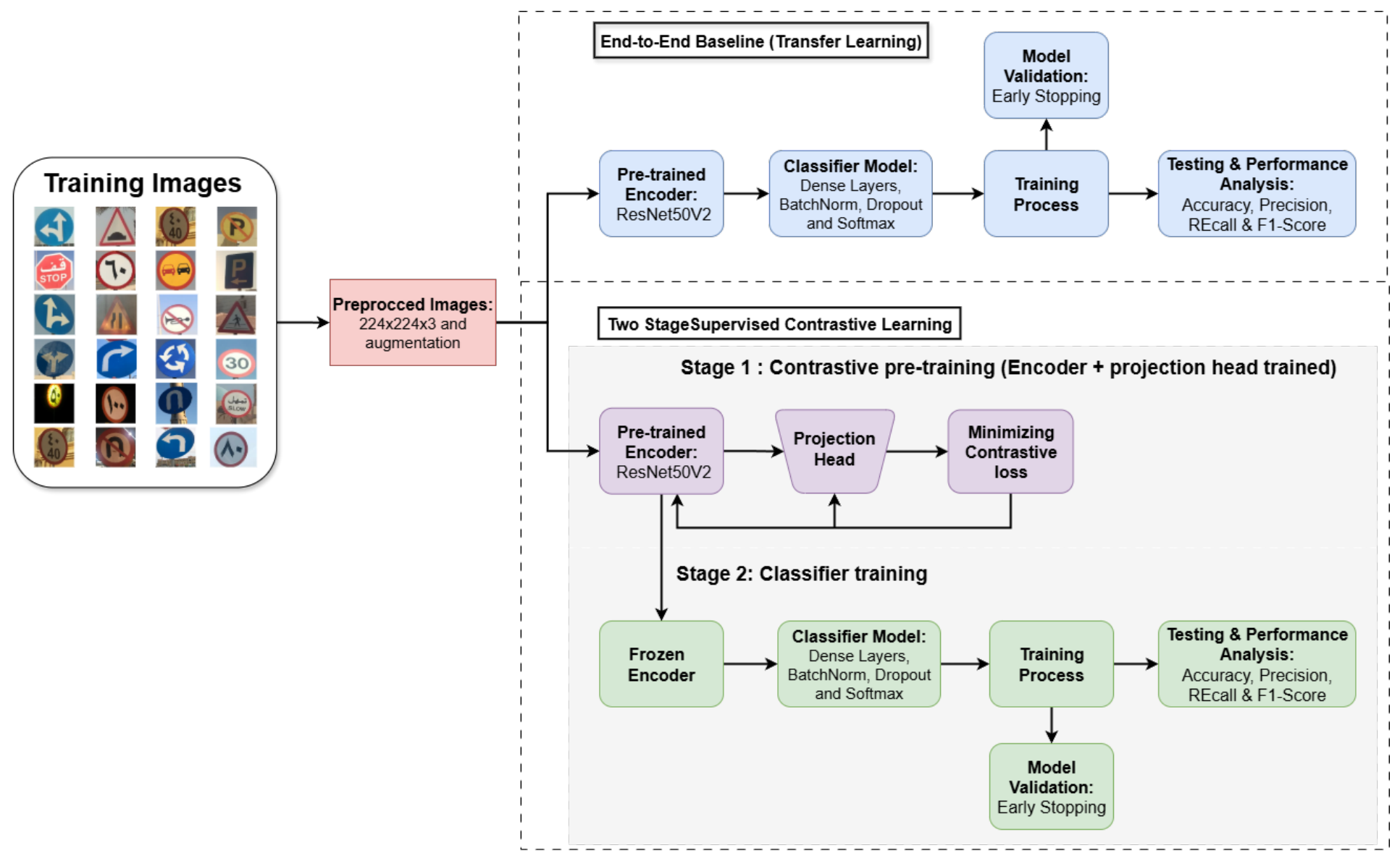
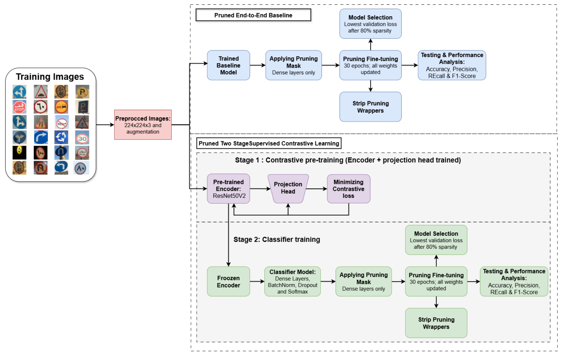
We investigate a two-stage supervised contrastive learning framework for Arabic traffic sign recognition and compare it with an end-to-end transfer learning baseline. Both approaches use a pre-trained encoder and a classifier network. In the first stage of the two-stage framework, the encoder and a projection head are trained by minimising the supervised contrastive loss to learn discriminative feature representations. The encoder weights are then frozen, and a new classifier is trained on the learned features using cross-entropy loss. To distinguish the effect of the contrastive objective from that of the two-stage training procedure, a cross-entropy two-stage control is also included. The overall architecture is illustrated in Figure 1. Furthermore, magnitude-based pruning is applied to the Dense layers to induce sparsity. The details of each module are provided in the following subsections.

Figure 1. Framework architecture of the end-to-end transfer learning baseline and the two-stage supervised contrastive learning approach.

3.1. Transfer Learning

Transfer learning is among the deep learning techniques that have been recently applied to solve complex tasks in natural language processing (NLP) and computer vision [67]. By utilising pre-trained parameters from large-scale datasets such as ImageNet [68], classification models can achieve improved performance. This is primarily accomplished by pre-training a network on a source domain and subsequently fine-tuning it on a related target domain to facilitate the learning of transferable feature embeddings. The widespread availability of open-source architectures pre-trained on ImageNet has led to the development of robust and computationally efficient baselines across multiple domains, including image classification and other computer vision tasks.

Our base model follows a two-module transfer learning architecture consisting of a pre-trained feature encoder and a task-specific classifier. The encoder module utilises ResNet50V2 to capture high-level feature representations from input images, serving as the main component of the recognition pipeline [69]. ResNet50V2 extends the original ResNet50 architecture by employing pre-activation residual units and identity shortcut connections to improve information and gradient propagation [69]. These residual connections ease the optimisation of very deep networks and address the degradation problem, in which the accuracy of plain networks deteriorates as depth increases, thereby improving the trainability of deep networks [70].

As shown in Table 2, ResNet50V2 begins with a stem consisting of a 7 × 7 convolutional layer with stride 2, which produces 112 × 112 feature maps, followed by a 3 × 3 max pooling layer with stride 2, which reduces the spatial resolution to 56 × 56. These are followed by four consecutive residual block stages (Stages II–V), each comprising several bottleneck residual blocks that employ the pre-activation paradigm, where batch normalisation and ReLU activation are applied before each convolutional operation. Throughout the network, identity shortcut connections allow gradients to propagate directly across layers, mitigating the vanishing gradient problem and enabling the training of very deep models. After the last residual stage, global average pooling transforms the 7 × 7 × 2048 feature maps into 2048-dimensional representations.

Table 2. Layer configuration of ResNet50V2 [69,70].

Layer Name (Stage)	Output Dimensions	Configuration
Initial Convolution (Stage I)	$112\times 112$	$7\times 7$ conv, stride 2
	$56\times 56$	$3\times 3$ max pool, stride 2
Residual Block Group (Stage II)	$56\times 56$	$\left[\begin{array}{c}1\times 1,64\hfill \\ 3\times 3,64\hfill \\ 1\times 1,256\hfill \end{array}\right]\times 3$
Residual Block Group (Stage III)	$28\times 28$	$\left[\begin{array}{c}1\times 1,128\hfill \\ 3\times 3,128\hfill \\ 1\times 1,512\hfill \end{array}\right]\times 4$
Residual Block Group (Stage IV)	$14\times 14$	$\left[\begin{array}{c}1\times 1,256\hfill \\ 3\times 3,256\hfill \\ 1\times 1,1024\hfill \end{array}\right]\times 6$
Residual Block Group (Stage V)	$7\times 7$	$\left[\begin{array}{c}1\times 1,512\hfill \\ 3\times 3,512\hfill \\ 1\times 1,2048\hfill \end{array}\right]\times 3$
Output Layer	$1\times 1$	Global average pooling ($7\times 7$)
		2048-dimensional feature vector

The encoder outputs are fed to a task-specific classifier module, which reduces the 2048-dimensional feature vectors to the final classification using a two-layer fully connected network. The first hidden layer has 512 units with ReLU activation, batch normalisation, and 50% dropout for regularisation. Subsequently, a second hidden layer further reduces the dimensionality to 256 units, with the same normalisation and dropout policy. The last layer has a softmax activation function with 24 output units that produces probability distributions over the 24 classes in our dataset. The classifier is trained with the Adam optimiser and the sparse categorical cross-entropy loss. The encoder can be used in two modes: (a) in the end-to-end baseline, the entire network (encoder and classifier) is updated during training; (b) in the two-stage models, the encoder is frozen and only the classification layers are trained. Additional implementation details are provided in Section 4.

3.2. Supervised Contrastive Learning

Our supervised contrastive learning (SCL) framework uses a two-stage training scheme that exploits class label information to learn discriminative features by optimising the contrastive loss. Unlike self-supervised contrastive learning methods, which produce positive pairs by comparing the augmented views of single images and treat all other samples in the batch as negatives, our supervised solution leverages class labels to provide more meaningful relationships among samples. In particular, positive pairs are formed by pairs of samples from the same class, while negative pairs are formed by pairs of samples from different classes. This label-driven approach is designed to promote intra-class compactness and inter-class separation in the embedding space [71].

Our SCL framework uses the same ResNet50V2 encoder architecture as the transfer learning baseline but follows a different training strategy. Whereas the baseline trains the encoder and classifier end-to-end using cross-entropy loss, SCL first trains the encoder and a projection head using supervised contrastive loss, followed by classifier training with the encoder weights frozen. This two-stage procedure allows the encoder to learn feature representations without being directly optimised for classification during the first stage. During contrastive training, the encoder is trained to bring anchor samples closer to positive samples (same class) and further from negative samples (different classes) in the embedding space. The similarity between two samples is measured using the cosine similarity of their projected embeddings:

$$\mathrm{sim}(z_i,z_j)={\displaystyle \frac{z_i·z_j}{\parallel z_i\parallel \parallel z_j\parallel }},$$

(1)

where $z_i$ and $z_j$ are the projection-head outputs, $z_i·z_j$ denotes the dot product of the two vectors, and $\parallel ·\parallel$ denotes the Euclidean (L2) norm. Since the embeddings are L2-normalised, the dot product between them is equivalent to cosine similarity.

Our supervised contrastive learning framework is broadly divided into four main components:

• Data Augmentation
  Data augmentation, $\mathrm{Aug}(·)$, produces random transformations $\tilde{x}=\mathrm{Aug}\left(x\right)$ of each input sample x to improve the generalisation and robustness of the model. We apply a series of geometric and photometric augmentations in our augmentation pipeline. The pipeline consists of normalisation, random width and height distortion ($\pm 10\%$), random zoom perturbation ($\pm 10\%$), random brightness distortion ($\pm 10\%$), and random contrast distortion ($\pm 10\%$). These transformations increase the diversity of the training samples while preserving their semantic content, helping the model to become less sensitive to visual variations.
• Base Encoder
  As explained earlier, our base encoder, $\mathrm{Enc}(·)$, uses a ResNet50V2 architecture pre-trained on ImageNet to capture high-level feature representations. The augmented input $\tilde{x}$ is then processed by the encoder and encoded into a 2048-dimensional representation vector:

  $$r=\mathrm{Enc}\left(\tilde{x}\right)\in {\mathbb{R}}^{2048}$$

  (2)
• Projection Head
  The projection head, $\mathrm{Proj}(·)$, is a lightweight network that projects the encoder representations into a lower-dimensional embedding space for contrastive learning. It consists of a Dense layer followed by ReLU and batch normalisation:

  $$z=\mathrm{BatchNorm}\left(\mathrm{ReLU}\left({\mathrm{Dense}}_{128}\left(r\right)\right)\right)\in {\mathbb{R}}^{128}$$

  (3)

  where the projection maps the 2048-dimensional encoder features to 128-dimensional embeddings. This dimensionality reduction provides a dedicated space for similarity comparisons during contrastive optimisation. The projection head is used only during contrastive pre-training and is then discarded, so that the classifier operates on the full 2048-dimensional encoder representation.
• Supervised Contrastive Loss
  The contrastive loss is calculated on the projected embeddings to learn the geometric structure of the feature space. Our supervised contrastive loss exploits class label information to define informative positive and negative pairs, where instances of the same class are pulled together and instances of different classes are pushed apart. The loss of the network is defined by the supervised contrastive loss function, as formulated in Equation (4).

  $$\begin{array}{cc}\hfill {\mathcal{L}}^{\sup }& =\sum _{i\in I}{\mathcal{L}}_i\hfill \\ \hfill {\mathcal{L}}_i& =-{\displaystyle \frac{1}{\left|P\right(i\left)\right|}}\sum _{p\in P\left(i\right)}\log {\displaystyle \frac{\exp (z_i·z_p/\tau )}{{\sum }_{a\in A\left(i\right)}\exp (z_i·z_a/\tau )}}\hfill \end{array}$$

  (4)
  In Equation (4), $P\left(i\right)\equiv \{p\in I:y_p=y_i,p\ne i\}$ is the set of all positive samples taken from the same class as anchor i but excluding the anchor itself, and $\left|P\right(i\left)\right|$ is the total number of positive samples in the batch for that class. $A\left(i\right)\equiv \{a\in I:a\ne i\}$ represents all samples in the batch excluding the anchor i itself, encompassing both positive samples (same class) and negative samples (different classes). This supervised framework is fundamentally different from self-supervised contrastive methods, which select positive and negative pairs based on views of the same image rather than on ground-truth class labels. The temperature $\tau$ controls how sharply the similarities are distributed, with lower values producing more confident predictions and tighter class clusters in the embedding space. In all experiments, $\tau =0.1$, and the loss is averaged over all anchors in the batch.

3.3. Cross-Entropy Two-Stage Control

To distinguish the effect of the supervised contrastive learning objective from that of the two-stage training procedure, we additionally train a cross-entropy (CE) two-stage control model. It uses the same ResNet50V2 encoder architecture, data augmentation, fixed 50-epoch first stage without early stopping, and second-stage training procedure as the SCL model. However, in the first stage, the encoder is trained using a linear softmax classification head and cross-entropy loss instead of the projection head and supervised contrastive loss. As in SCL, the first-stage head is then discarded, the encoder is frozen, and the same classifier architecture is trained in the second stage. This controlled comparison allows us to examine whether the performance differences are associated with the first-stage learning objective under a matched two-stage training procedure.

3.4. Pruning

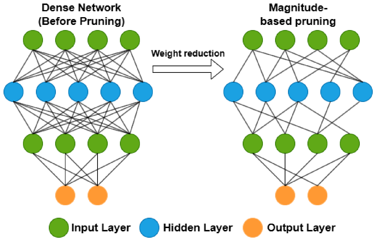
In Intelligent Transportation Systems (ITS), where computational and memory resources are often constrained, model compression is important for reducing memory and computational requirements while maintaining predictive accuracy. We use TensorFlow’s magnitude-based unstructured pruning framework, which ranks weights by their absolute magnitude and zeroes out the smallest values until reaching a target sparsity level [72]. A visual representation of the magnitude-based unstructured pruning process is shown in Figure 2. To preserve the convolutional feature extraction layers, we apply magnitude-based pruning only to Dense layers while keeping all convolutional layers unpruned. This approach preserves the network architecture and maintains the same total number of parameters, with pruned weights set to zero instead of being structurally removed. To stabilise training and avoid sudden weight removal, the sparsity progression follows a polynomial decay schedule:

$$S\left(t\right)=S_{\mathrm{final}}+(S_{\mathrm{initial}}-S_{\mathrm{final}})\times {\left(1-{\displaystyle \frac{t}{T}}\right)}^p$$

(5)

where $S\left(t\right)$ represents the sparsity level at training step t, T denotes the number of steps over which sparsity is increased, and p is the polynomial power. The pruning threshold is determined separately for each Dense layer l from the magnitudes of its kernel weights $W^{\left(l\right)}$:

$$q_{\lambda }^{\left(l\right)}:=quantile\left(\left\{|w_i^{\left(l\right)}|:w_i^{\left(l\right)}\in W^{\left(l\right)}\right\};\lambda \right),$$

(6)

where $\lambda =S\left(t\right)$. The pruning operation is defined as:

$$w_{i,\lambda }^{\left(l\right)}=\left\{\begin{array}{cc}0,\hfill & \mathrm{if}|w_i^{\left(l\right)}|\le q_{\lambda }^{\left(l\right)},\hfill \\ w_i^{\left(l\right)},\hfill & \mathrm{otherwise},\hfill \end{array}\right.l\in \mathcal{D},$$

(7)

$\mathcal{D}$ denotes the set of Dense layers selected for pruning. This operation sets a fraction $\lambda$ of the kernel weights in each Dense layer to zero, while leaving bias terms unpruned.

Figure 2. Illustration of magnitude-based unstructured pruning [73]. The original dense network (left) contains all connections, while the pruned sparse network (right) shows reduced connectivity after eliminating low-magnitude weights.

In our experiments, sparsity increases from an initial value of 30% to a final value of 80% over the first 20 of 30 fine-tuning epochs, with a polynomial power of 3. The pruning masks are updated every 100 training steps, and the target sparsity is maintained during the remaining epochs. Model selection is restricted to epochs after the target sparsity has been reached, based on the lowest validation loss. During fine-tuning, the end-to-end baseline updates both the encoder and classifier, whereas the two-stage models keep their encoders frozen and update only their classifier heads. After fine-tuning, the pruning wrappers are removed, preserving the original network architecture and total parameter count while retaining the pruned weights as zeros. Figure 3 illustrates the overall architecture of the proposed pruning framework.

Figure 3. Framework architecture of the pruned end-to-end baseline and the pruned two-stage supervised contrastive learning approach.

4. Experimental Results

This section presents the dataset, evaluation metrics and implementation settings, followed by the multi-seed classification results, an ablation study of the training objective, the model size and computational cost analysis, a comparison with previously reported methods, and an error analysis.

4.1. Dataset

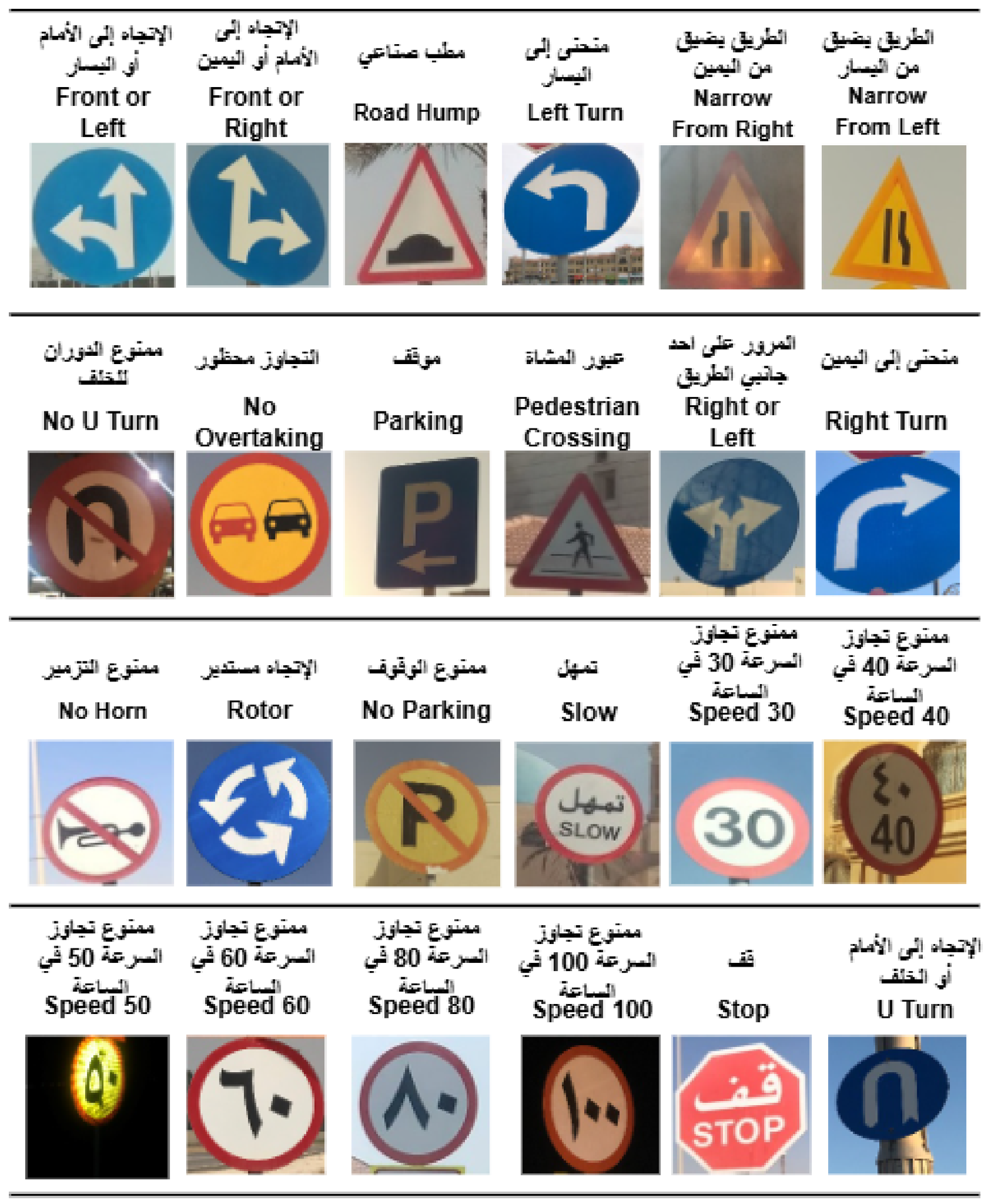
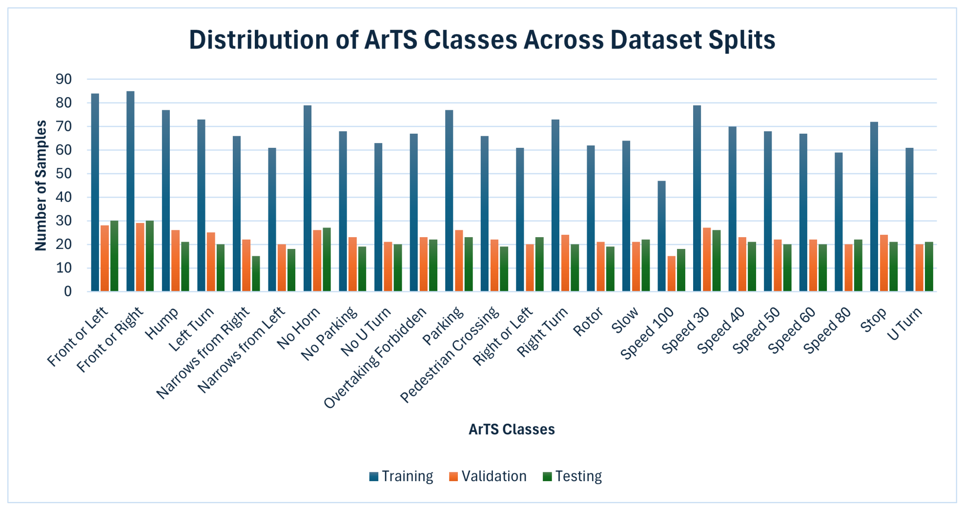
This study uses the Arabic traffic sign (ArTS) dataset developed at Prince Mohammad Bin Fahd University in Al Khobar, Kingdom of Saudi Arabia [74]. It is an open-source dataset for research on traffic sign recognition and autonomous vehicle applications. It was created to address the lack of resources for Arabic traffic sign recognition and supports applications such as autonomous vehicle navigation, intelligent traffic monitoring and driving safety. The ArTS dataset is a collection of 2718 images representing the 24 Arabic traffic signs most frequently encountered in Saudi Arabia, as shown in Figure 4. These images were systematically collected from three neighbouring cities, Al Khobar, Dammam and Dhahran, to ensure broad representation. In the original release, the dataset is split into 2200 training and 518 test images. For this study, the 2200 training images are further divided into 1650 training and 550 validation images using stratified sampling with a fixed random seed, while the original 518 test images remain unchanged (Figure 5). This split is performed only once and remains consistent across all experimental runs. The validation set is used for early stopping and model selection, whereas all reported performance results are obtained from the test set.

Figure 4. Examples of Arabic traffic signs (modified from ArTS dataset [74]).

Figure 5. Class distribution of the 24 traffic sign classes in the training, validation and test sets of the ArTS dataset.

4.2. Evaluation Metrics

The performance of the proposed models was assessed using the standard evaluation metrics, namely accuracy, precision, recall, F1-score. Accuracy measures the proportion of correctly recognised traffic signs out of all samples, providing an intuitive overall assessment of performance.

$$\begin{array}{cc}\hfill \mathrm{Accuracy}& ={\displaystyle \frac{1}{N}}{\displaystyle \sum _{c=1}^C}T{P}_c,\hfill \end{array}$$

(8)

$$\begin{array}{cc}\hfill {\text{F1-score}}_c& =2·{\displaystyle \frac{{\mathrm{Precision}}_c\times {\mathrm{Recall}}_c}{{\mathrm{Precision}}_c+{\mathrm{Recall}}_c}},\hfill \end{array}$$

(9)

where

$$\begin{array}{cc}\hfill {\mathrm{Precision}}_c& ={\displaystyle \frac{T{P}_c}{T{P}_c+F{P}_c}},\hfill \end{array}$$

(10)

$$\begin{array}{cc}\hfill {\mathrm{Recall}}_c& ={\displaystyle \frac{T{P}_c}{T{P}_c+F{N}_c}}.\hfill \end{array}$$

(11)

where $T{P}_c$, $F{P}_c$ and $F{N}_c$ denote the numbers of true positives, false positives and false negatives for class c in a one-vs.-rest evaluation. Here, $C=24$ represents the number of classes, and N denotes the total number of test images. Accuracy measures the proportion of correctly classified images, while precision, recall and F1-score are calculated separately for each class and then averaged across all classes, weighted by the number of test images in each class.

However, accuracy may not adequately represent the classifier’s efficacy in cases with substantial class imbalance. Precision measures the proportion of correct positive predictions relative to all positive predictions, while recall measures the proportion of true positives relative to all actual positive instances. The F1-score, defined as the harmonic mean of precision and recall, accounts for both false positives and false negatives. This makes it particularly relevant for Arabic traffic sign recognition, where some sign categories occur less frequently than others.

4.3. Evaluation Protocol and Statistical Analysis

All models are trained and evaluated using the data split described in Section 4.1. To assess the stability of the results, the main configurations (baseline, SCL, CE two-stage, and their pruned versions) are each trained with ten different random seeds (0–9), which affect weight initialisation, data augmentation, and batch order. The frozen-ImageNet control and the re-trained models from previous studies are also evaluated using multiple random seeds. Results are reported as mean ± standard deviation across seeds. Pairwise differences between configurations are assessed using two-sided paired t-tests and Wilcoxon signed-rank tests on test accuracies obtained from matched random seeds, with a significance level of 0.05. A non-significant result indicates no statistically detectable difference under the evaluated conditions and does not establish equivalence. The reported p-values are not adjusted for multiple comparisons.

4.4. Implementation Details

Following the methodology described in Section 3, we evaluate four main configurations: the end-to-end transfer learning baseline, the pruned baseline, two-stage supervised contrastive learning (SCL), and pruned SCL. To examine the effect of the first-stage training configuration under a matched two-stage procedure, we additionally evaluate the cross-entropy (CE) two-stage control and its pruned version (Section 3.3), as well as a frozen-ImageNet control, in which the ImageNet-pretrained encoder is kept frozen and only the classifier is trained. All ResNet50V2-based configurations use an ImageNet-pretrained encoder with input images of 224 × 224 × 3 pixels. The common training settings are as follows, with stage-specific differences described below:

• Batch size: 16
• Learning rate: $1\times {10}^{-4}$
• Optimiser: Adam
• Cross-entropy classifier training (baseline and second stages): up to 50 epochs with early stopping (patience of 8 epochs based on the validation loss, restoring the best weights)

In the baseline configuration, the encoder and classifier are trained end-to-end using the shared hyperparameters listed above and the sparse categorical CE loss. The SCL configuration begins by training the encoder together with the projection head (a 128-unit Dense layer with ReLU activation and batch normalisation) using the supervised contrastive loss with a temperature of 0.1 for a fixed 50 epochs, without early stopping. During the second stage, the projection head is discarded, the encoder is frozen, and the classifier is trained with the CE loss using the settings listed above. The CE two-stage control follows the same schedule, including a fixed 50-epoch first stage without early stopping, but uses a linear softmax head and the CE loss instead of the projection head and the supervised contrastive loss in the first stage. The same batch size, learning rate and optimiser are used in all training stages, including contrastive pre-training and pruning fine-tuning.

The pruned configurations are initialised from their corresponding trained models. Magnitude-based unstructured pruning is applied exclusively to the Dense layers over 30 fine-tuning epochs. Sparsity gradually increases from 30% to 80% during the first 20 epochs, using a polynomial decay schedule with a power of 3 and pruning masks updated every 100 training steps. The target sparsity of 80% is then maintained for the remaining epochs. Rather than applying early stopping, the model with the lowest validation loss is selected from the epochs after the target sparsity has been reached. All reported pruned models achieved 80.0% sparsity in their Dense-layer kernels, corresponding to approximately 3.8% sparsity across all model parameters, as the convolutional layers remain unpruned. During pruning fine-tuning, the baseline model updates both the encoder and classifier weights, whereas the two-stage models retain their frozen encoders and update only the classifier weights.

All experiments were carried out on a computer system equipped with an AMD Ryzen 7 5800H central processing unit (CPU), 16 GB of random-access memory (RAM), and an NVIDIA GeForce RTX 3060 Laptop graphics processing unit (GPU) with 6 GB of dedicated memory. The implementation was developed using TensorFlow 2.10 as the primary deep learning framework. Model pruning was carried out with the TensorFlow Model Optimization Toolkit (version 0.8), while evaluation metrics and statistical tests were computed using scikit-learn (version 1.7.2) and SciPy (version 1.10.1), respectively.

4.5. Measurement of Model Size and Inference Cost

To ensure consistent model size measurements, all models are saved in the same format without optimiser states. We report the sizes of the weights-only HDF5 files, their gzip-compressed versions, and the float32 and full-integer int8 TensorFlow Lite models. For int8 quantisation, 100 training images are used as a representative dataset to calibrate activation ranges. Model sizes are reported in decimal megabytes (1 MB = ${10}^6$ bytes), while computational complexity is measured in floating-point operations (FLOPs) of the inference graph. The inference benchmarking settings are summarised in Table 3.

Table 3. Inference benchmarking configurations.

Framework	Device	Measured Runs	Warm-Up Runs
TensorFlow	GPU	200	20
TensorFlow	CPU	200	20
TensorFlow Lite (float32)	CPU	100	10
TensorFlow Lite (int8)	CPU	3	1

All latency measurements are conducted with a batch size of one and reported as the median inference time. Both TensorFlow Lite models are evaluated on the same CPU under identical runtime settings, using 16 CPU threads. Peak GPU memory usage during inference is also recorded. Due to the long per-image runtime, int8 latency is measured over only three runs and is therefore considered indicative rather than a precise benchmark. Since unstructured pruning retains the dense computational graph, reductions in FLOPs or inference latency are not expected without sparse execution support. Latency and memory measurements are performed using the first random seed, while agreement between int8 and float32 predictions is assessed on a class-stratified subset of 120 test images (five per class).

4.6. Results and Discussion

This subsection presents the experimental results and discusses the classification performance, ablation study, model size and computational cost, comparison with previous studies, and error analysis.

4.6.1. Classification Results

We present the classification performance of the four main configurations evaluated over ten random seeds in Table 4. The end-to-end baseline achieved a mean accuracy of 98.47 ± 0.28%, while the two-stage SCL model achieved 98.90 ± 0.50%, representing a paired mean improvement of 0.42 percentage points (pp) (paired t-test, $p=0.016$; Wilcoxon signed-rank test, $p=0.033$). SCL outperformed the baseline in seven of the ten seeds, with one tie. Although SCL achieved a higher mean accuracy, its larger standard deviation indicates greater variability across random seeds. The weighted precision and F1-score followed a similar pattern, consistent with the accuracy results. In terms of classification errors, SCL reduced the average number of misclassified images from 7.9 to 5.7 out of 518 test images per run. All reported p-values are unadjusted for multiple comparisons (Section 4.3).

Table 4. Classification performance of the four main configurations on the ArTS test set (%; mean ± SD over 10 random seeds). Errors are the number of misclassified test images per run (out of 518).

Method	Accuracy	Precision	Recall	F1-Score	Errors
End-to-end baseline	98.47 ± 0.28	98.58 ± 0.25	98.47 ± 0.28	98.48 ± 0.28	7.9 ± 1.4
Pruned baseline	99.07 ± 0.27	99.14 ± 0.24	99.07 ± 0.27	99.07 ± 0.27	4.8 ± 1.4
SCL two-stage	98.90 ± 0.50	98.96 ± 0.48	98.90 ± 0.50	98.90 ± 0.50	5.7 ± 2.6
Pruned SCL	99.00 ± 0.54	99.07 ± 0.46	99.00 ± 0.54	99.00 ± 0.52	5.2 ± 2.8

Precision, recall and F1-score are weighted by the number of test images per class; weighted recall therefore equals accuracy.

Regarding the effect of magnitude-based pruning, applying 80% sparsity to the Dense-layer weights preserved classification performance in both main configurations. For the baseline, mean accuracy increased from 98.47% to 99.07%, representing a paired improvement of 0.60 ± 0.31 pp (paired t-test, $p<0.001$; Wilcoxon signed-rank test, $p=0.004$), with higher accuracy in nine of the ten seeds and one tie. In contrast, SCL showed a smaller improvement of 0.10 ± 0.25 pp, which was not statistically significant ($p=0.25$). The difference between the pruned SCL and pruned baseline models was also not statistically significant ($-0.08$ pp, $p=0.67$). Two factors may contribute to the observed accuracy improvement. First, magnitude-based pruning removes weights with small absolute values, reducing the effective complexity of the Dense layers while retaining the remaining connections. This may act as a form of regularisation by limiting overfitting and improving generalisation to unseen data. However, the same Dense layers were pruned to 80% sparsity in the two-stage models without a significant change in accuracy, suggesting that this potential regularisation effect alone does not explain the larger improvement in the baseline. Second, pruning involved 30 additional epochs of fine-tuning, during which the baseline continued updating both the ResNet50V2 encoder and classifier, whereas the two-stage models updated only their classifiers with frozen encoders. This additional end-to-end optimisation may have allowed the baseline to refine its feature representations further, contributing to its larger accuracy improvement. However, because sparsity and fine-tuning were applied together, their individual contributions to the observed improvement cannot be determined from these experiments. Nevertheless, the results demonstrate that 80% sparsity in the Dense layers can be achieved while maintaining classification performance.

To further examine the classification results, Table 5 presents the true positive (TP), true negative (TN), false positive (FP) and false negative (FN) counts for each configuration, summed across the 24 classes using a one-vs.-rest approach. The results are reported as the mean and standard deviation over ten random seeds. In this multi-class setting, each misclassified image contributes one FP to the predicted class and one FN to the actual class. Consequently, the total FP and FN counts are equal and correspond to the classification errors reported in Table 4. The relatively large TN counts arise because each test image is treated as a negative example for the other 23 classes. The per-class results for the SCL model, including precision, recall and F1-score, are discussed in Section 4.6.5.

Table 5. True positive (TP), true negative (TN), false positive (FP) and false negative (FN) counts per test run (518 images), summed over the 24 classes in a one-vs.-rest manner (mean ± SD over 10 random seeds). These counts underlie the metrics in Table 4 (Equations (8)–(11)).

Method	TP	TN	FP	FN
End-to-end baseline	510.1 ± 1.4	11,906.1 ± 1.4	7.9 ± 1.4	7.9 ± 1.4
SCL two-stage	512.3 ± 2.6	11,908.3 ± 2.6	5.7 ± 2.6	5.7 ± 2.6
CE two-stage	512.7 ± 1.8	11,908.7 ± 1.8	5.3 ± 1.8	5.3 ± 1.8
Pruned baseline	513.2 ± 1.4	11,909.2 ± 1.4	4.8 ± 1.4	4.8 ± 1.4
Pruned SCL	512.8 ± 2.8	11,908.8 ± 2.8	5.2 ± 2.8	5.2 ± 2.8
Pruned CE two-stage	512.6 ± 1.8	11,908.6 ± 1.8	5.4 ± 1.8	5.4 ± 1.8

In a multi-class setting, each misclassified image counts as one FN for its true class and one FP for the predicted class; therefore, the summed FP and FN are equal. TP + TN + FP + FN = 24 × 518 = 12,432 per run.

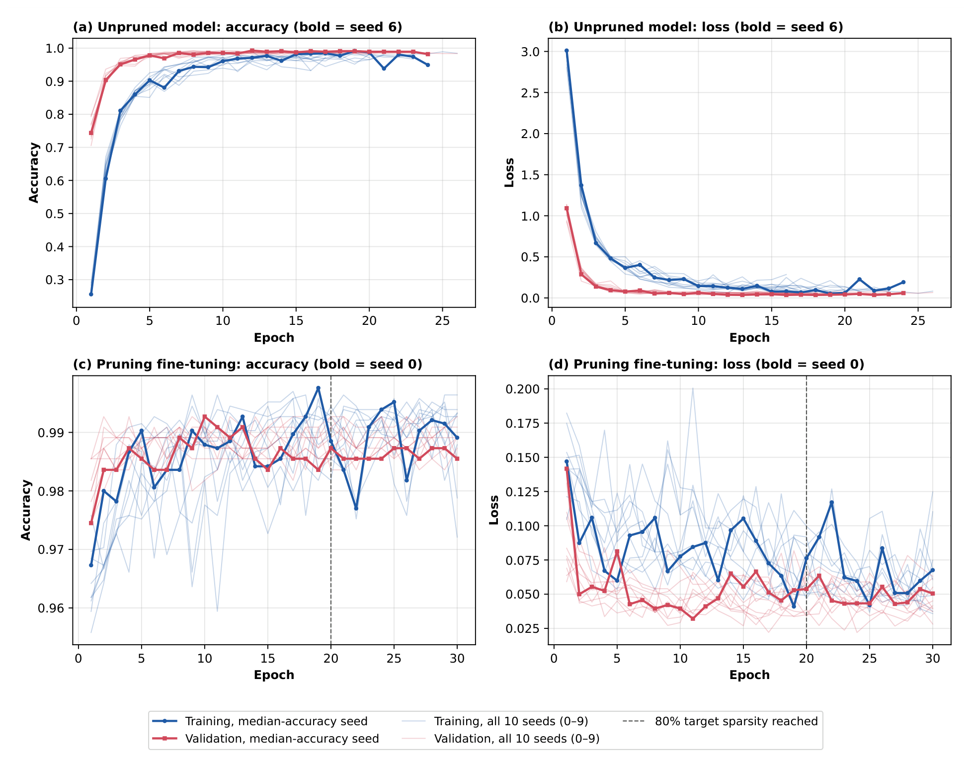
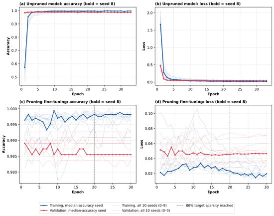
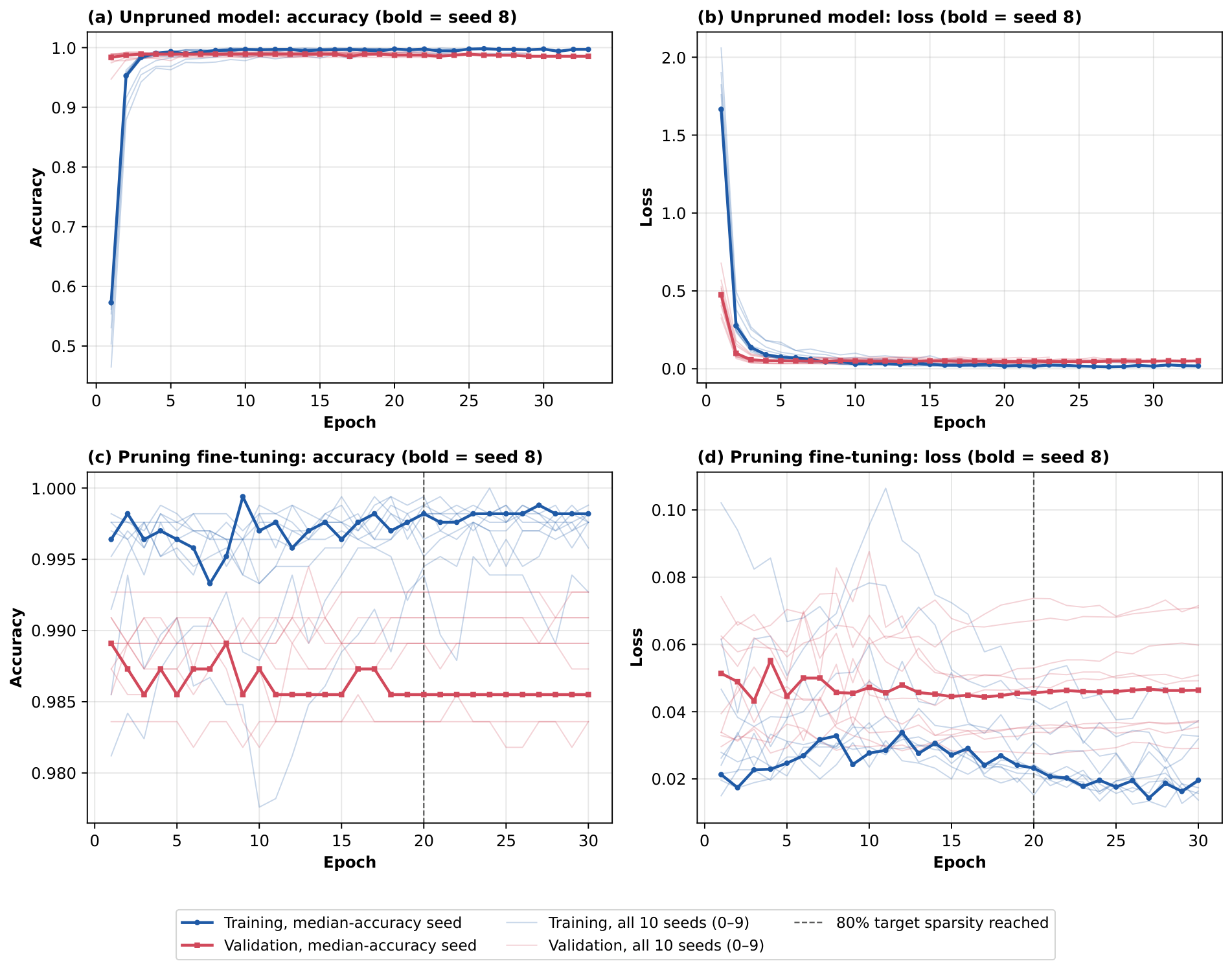
Figure 6 and Figure 7 show the training and validation curves of the baseline and SCL models over the ten seeds. For the baseline, the validation loss reached its minimum after 8–18 epochs, after which early stopping ended training. The training accuracy remained below the validation accuracy during most epochs because it was computed with data augmentation and dropout active. For SCL, the second-stage classifier reached a validation accuracy of approximately 98–99% within the first epochs, because the encoder had already been trained in the contrastive stage and only the classifier was updated. During pruning fine-tuning (Figure 6c,d and Figure 7c,d), the validation accuracy of both models remained within a narrow range while the sparsity increased from 30% to 80% and after the target sparsity was reached, indicating that removing 80% of the Dense-layer weights did not degrade recognition performance.

Figure 6. Training and validation curves of the end-to-end baseline over ten random seeds (0–9): (a,b) training of the unpruned model and (c,d) pruning fine-tuning. Curve lengths in (a,b) differ between seeds because of early stopping. Training accuracy is computed with data augmentation and dropout active.

Figure 7. Training and validation curves of the SCL model over ten random seeds (0–9): (a,b) second-stage classifier training with the encoder frozen and (c,d) pruning fine-tuning. Curve lengths in (a,b) differ between seeds because of early stopping.

4.6.2. Ablation Study: Effect of the Training Objective

The comparison in Section 4.6.1 differs in two respects: the training objective of the encoder (supervised contrastive loss versus cross-entropy) and the training procedure (two-stage training with a frozen encoder versus end-to-end training). To determine which of these factors is associated with the improvement, we compared SCL with the CE two-stage control (Section 3.3), which follows the same two-stage procedure and schedule but uses a linear softmax classification head and the cross-entropy loss instead of the projection head and the supervised contrastive loss in the first stage, and with a frozen-ImageNet control, in which the encoder is not trained on ArTS. The results are summarised in Table 6 and Table 7.

Table 6. Ablation study on the ArTS test set (%; mean ± SD over random seeds). All configurations use the same ResNet50V2 encoder, classifier and data split.

Configuration	Encoder Training	Accuracy	Macro F1
Frozen ImageNet	None (ImageNet weights)	88.22 ± 0.61	87.96 ± 0.56
End-to-end baseline	End-to-end, CE	98.47 ± 0.28	98.46 ± 0.27
CE two-stage	Stage 1, CE	98.98 ± 0.34	98.96 ± 0.35
SCL two-stage	Stage 1, SCL	98.90 ± 0.50	98.86 ± 0.53
Pruned CE two-stage	Stage 1, CE	98.96 ± 0.34	98.93 ± 0.33
Pruned SCL	Stage 1, SCL	99.00 ± 0.54	98.94 ± 0.61

Table 7. Paired comparisons of test accuracy over matched random seeds ($\mathrm{\Delta }$ = first minus second configuration, in percentage points; mean ± SD). Wins: number of seeds in which the first configuration was more accurate. p-values are two-sided and unadjusted for multiple comparisons.

Comparison	$\mathbf{\Delta }$ (pp)	t-Test p	Wilcoxon p	Wins
SCL vs. end-to-end baseline	+0.42 ± 0.45	0.016	0.033	7/10 (1 tie)
CE two-stage vs. end-to-end baseline	+0.50 ± 0.39	0.003	0.006	9/10
SCL vs. CE two-stage	−0.08 ± 0.38	0.534	0.375	4/10
SCL vs. frozen ImageNet	+10.69 ± 0.62	<0.001	0.062 1	5/5
Pruned SCL vs. pruned baseline	−0.08 ± 0.56	0.674	0.770	5/10
Pruned SCL vs. pruned CE two-stage	+0.04 ± 0.42	0.775	0.888	4/10 (2 ties)

¹ With five pairs, 0.0625 is the smallest two-sided p-value attainable by the Wilcoxon signed-rank test.

The frozen-ImageNet control achieved an accuracy of 88.22%, approximately 10.7 pp below SCL (Table 7), indicating that adapting the encoder to Arabic traffic signs substantially improves classification performance compared with using frozen ImageNet features. The CE two-stage control achieved 98.98 ± 0.34%, significantly outperforming the end-to-end baseline (+0.50 pp, paired t-test, $p=0.003$), while showing no statistically significant difference from SCL ($-0.08$ pp, $p=0.53$). These findings suggest that the improvement over the end-to-end baseline is associated with the two-stage training configuration, while no additional statistically significant advantage of SCL over the CE two-stage control was detected. However, two limitations should be considered. First, a non-significant difference does not establish equivalence, and the limited number of seeds may reduce the statistical power to detect small performance differences. Second, the two-stage configurations involved more gradient updates than the end-to-end baseline (approximately 7700 and 7600 versus 2100 steps), preventing a clear separation of the effects of the training procedure and the larger training budget. After pruning, SCL and CE two-stage continued to show similar performance ($p=0.78$), with only marginal changes in accuracy (SCL: +0.10 pp; CE two-stage: $-0.02$ pp).

4.6.3. Model Compression and Inference Efficiency

Table 8 summarises the model size and inference cost of the four main configurations, measured as described in Section 4.5. All four models share the same architecture and parameter count (24.75 million). When the models were saved in the same weights-only format, their file sizes were identical (99.35 MB). The size of a saved Keras model depends strongly on whether the optimiser state is stored: with the Adam optimiser state, the end-to-end model, whose encoder is trainable, occupies 297.45 MB, whereas a two-stage model with a frozen encoder occupies 108.88 MB, because optimiser moments are stored only for trainable weights. Such differences in file size are therefore caused by the serialisation format, not by the training method, and all comparisons below use the weights-only format.

Table 8. Model size and inference cost of the four main configurations (sizes in MB = ${10}^6$ bytes; median latency at batch size one; latency and memory measured for seed 0).

Metric	Baseline	Pruned Baseline	SCL	Pruned SCL
Total parameters (M)	24.75	24.75	24.75	24.75
Non-zero parameters (M)	24.75	23.81	24.75	23.81
Sparsity: Dense kernels/whole model (%)	0/0	80.0/3.8	0/0	80.0/3.8
Weights-only HDF5 (MB)	99.35	99.35	99.35	99.35
Weights-only HDF5, gzip (MB)	92.04	88.88	92.01	88.91
TFLite float32 (MB)	98.85	98.85	98.85	98.85
TFLite int8 (MB)	25.48	25.48	25.48	25.48
TFLite int8, gzip (MB)	21.14	20.51	21.19	20.43
int8–float32 agreement (%, 120 images)	99.2	100.0	100.0	100.0
FLOPs per image (G)	6.97	6.97	6.97	6.97
Latency, GPU, TensorFlow (ms)	6.5	9.0	5.8	6.0
Latency, CPU, TensorFlow (ms)	86.2	176.9	97.2	178.4
Latency, CPU, TFLite float32 (ms)	24.8	31.8	18.7	18.6
Latency, CPU, TFLite int8 (s) 1	2.68	2.97	2.70	2.75
Peak GPU memory (MB)	776	1023	720	800

¹ Median of three runs; indicative only (see Section 4.5).

The Dense layers account for 4.8% of all model parameters. Removing 80% of their weights (approximately 0.95 million weights) therefore resulted in an overall model sparsity of approximately 3.8%. Because unstructured pruning retains zero-valued weights in the dense format, it did not change the uncompressed file sizes but reduced the gzip-compressed model sizes by approximately 3.4% (92.04 to 88.88 MB for the baseline and 92.01 to 88.91 MB for SCL). The gzip-compressed int8 models also showed reductions of 3.0–3.6% after pruning, with the pruned SCL model achieving the smallest file size of 20.43 MB. In comparison, full-integer int8 quantisation reduced the model size by approximately 74% (99.35 to 25.48 MB), with 99.2–100% prediction agreement between the int8 and float32 models on 120 evaluated test images. These results highlight the complementary roles of pruning and quantisation in improving model storage efficiency.

All models had the same theoretical computational complexity of 6.97 GFLOPs per image, since unstructured pruning does not change the computational graph. Notably, SCL and pruned SCL showed GPU inference latencies of 5.8 and 6.0 ms, respectively, compared with 6.5 ms for the end-to-end baseline. This indicates that pruned SCL maintained comparable GPU inference performance while achieving 80% sparsity in the Dense layers. Overall, magnitude-based pruning preserved high classification accuracy while introducing substantial sparsity in the targeted Dense layers and providing modest compressed-storage savings. Further improvements in computational efficiency may be achieved by extending pruning to the convolutional encoder, which contains approximately 95% of the model parameters and accounts for nearly all computational operations, particularly through structured channel or filter pruning that removes complete operations from the computational graph.

4.6.4. Comparison with Previous Studies

Table 9 compares our results with previously reported methods on the ArTS dataset. Part (A) lists the accuracies reported in the original studies. In [40], network complexity in ResNet V1 was regulated by repeatedly stacking residual blocks, yielding a test accuracy of 96.14%. The LE-CNN model [65], comprising three convolutional blocks with dropout layers and trained on 32 × 32 RGB images, achieved 96.50% accuracy. In [41], a comparative evaluation of six architectures using extensive data augmentation and 5-fold cross-validation identified DenseNet121 as the best model, with a test accuracy of 96.54%. Because these results were obtained with different data splits, preprocessing and training settings, they cannot be compared directly with ours. Therefore, we re-trained ResNet V1 (ResNet50), DenseNet121 and LE-CNN under the protocol of this study (Part (B); Section 4).

Table 9. Comparison with previous methods on the ArTS test set. (A) Accuracy as reported in the original studies (different protocols; not directly comparable). (B) Methods re-trained under the protocol of this study (mean ± SD over random seeds).

Method	Accuracy (%)	Seeds
(A) Reported in previous studies
ResNet V1 [40]	96.14	–
LE-CNN [65]	96.50	–
DenseNet121 [41]	96.54	–
(B) Re-trained under the protocol of this study
LE-CNN 1	92.51 ± 0.54	5
ResNet V1 (ResNet50)	98.42 ± 0.60	5
DenseNet121	98.65 ± 0.47	5
ResNet50V2 end-to-end baseline	98.47 ± 0.28	10
Pruned ResNet50V2 baseline	99.07 ± 0.27	10
CE two-stage	98.98 ± 0.34	10
SCL two-stage	98.90 ± 0.50	10
Pruned SCL	99.00 ± 0.54	10

¹ Approximate re-implementation; some architectural details are not specified in [65].

Under the same protocol, ResNet50 (98.42%) and DenseNet121 (98.65%) achieved accuracies comparable to our ResNet50V2 baseline (98.47%) and approximately 2 pp higher than those reported in their original studies. The LE-CNN re-implementation achieved an accuracy of 92.51%, lower than the originally reported 96.50%. These findings suggest that differences in experimental protocols may contribute substantially to variations in reported accuracy, highlighting the importance of evaluating models under consistent conditions. Notably, both pruned configurations achieved higher mean accuracies than the re-trained ResNet50 and DenseNet121 models, reaching 99.07% for the pruned ResNet50V2 baseline and 99.00% for the pruned SCL model. Before pruning, the SCL model achieved a mean accuracy of 98.90%, which increased slightly to 99.00% after magnitude-based pruning. These results highlight the competitive recognition performance of the proposed SCL-based approach and its ability to maintain high classification accuracy under 80% Dense-layer sparsity.

4.6.5. Error Analysis

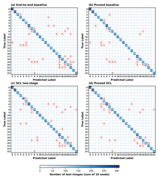
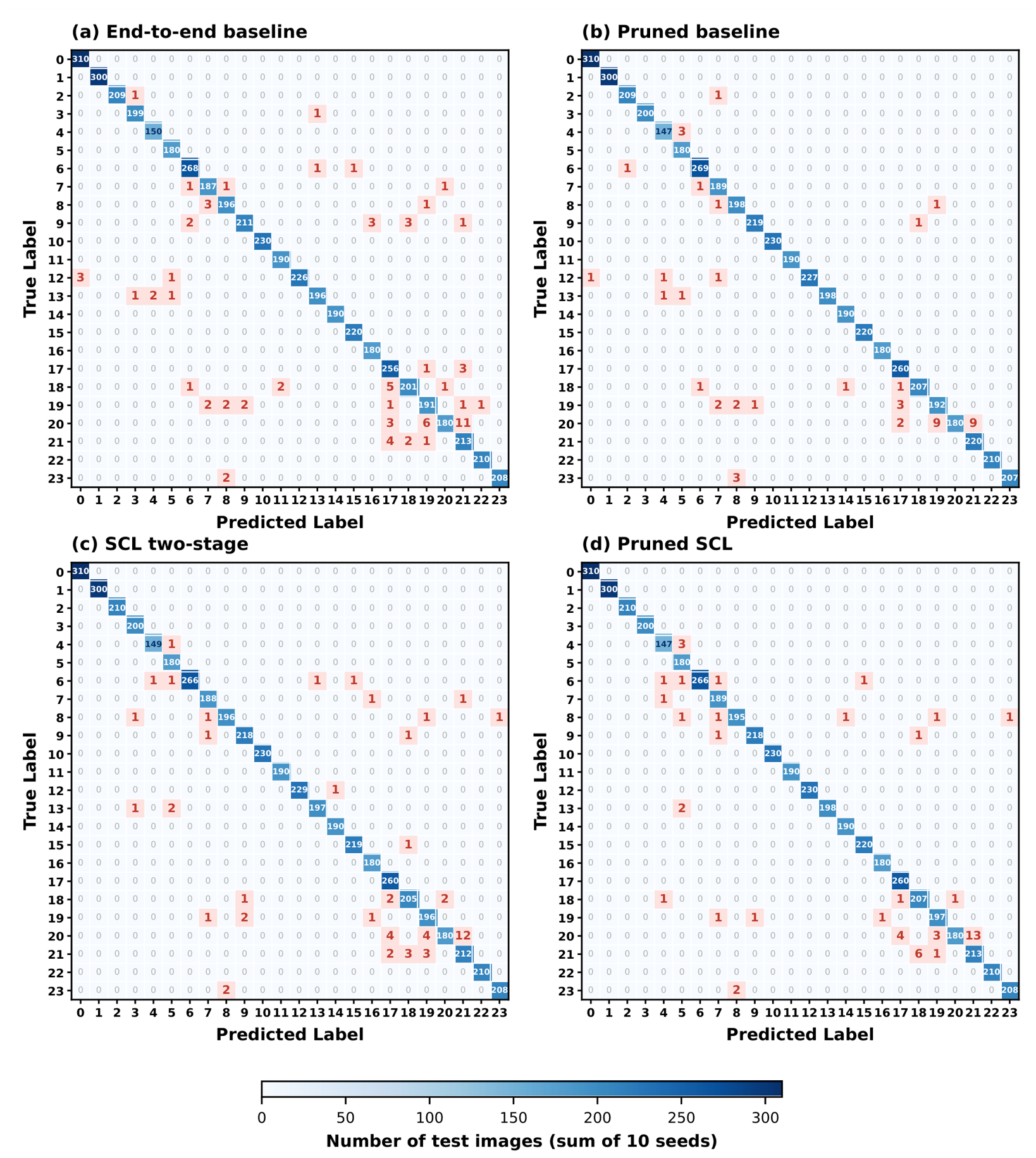
Table 10 presents the per-class TP, TN, FP and FN counts for the SCL model, while Figure 8 shows the confusion matrices of the four main configurations, aggregated across ten random seeds to illustrate their classification error patterns. Across all configurations, most classes were recognised without errors or with fewer than one error per run on average. For SCL, six classes (Front or Left, Front or Right, Hump, Parking, Pedestrian Crossing and Stop) had no FP or FN across any of the ten seeds. The classification errors were primarily concentrated among the speed-limit signs, classes 17–21 (Speed 30, Speed 40, Speed 50, Speed 60 and Speed 80), which share the same circular shape, colour and layout but differ in their displayed speed values. Confusions within this group accounted for 32 of the 57 SCL errors (56%) and 39 of the 79 baseline errors (49%). The most frequent misclassification involved Speed 60 being predicted as Speed 80, occurring 11, 9, 12 and 13 times over ten seeds for the baseline, pruned baseline, SCL and pruned SCL models, respectively; for the pruned baseline, this was tied with Speed 60 being predicted as Speed 50. For SCL, Speed 60 had the lowest recall (90.0%, corresponding to 2.0 FN per run), while Speed 80 had the lowest precision (94.2%, corresponding to 1.3 FP per run). In the one-vs.-rest evaluation, correct rejections (TNs) were the most frequent outcome for every class. For example, Speed 80 had an average of 494.7 TNs and 1.3 FPs per run among the 496 test images belonging to other classes, with 12 of the 13 FPs accumulated over ten seeds originating from Speed 60. This indicates that false positives for Speed 80 were primarily associated with the visually similar Speed 60 sign rather than being distributed across unrelated classes. Outside the speed-limit group, recurring confusions occurred mainly between signs with closely related pictograms, such as U Turn predicted as No U Turn (two to three times over ten seeds in every configuration) and the mirrored signs Narrows from Right predicted as Narrows from Left. Magnitude-based pruning reduced the total number of classification errors from 79 to 48 for the baseline and from 57 to 52 for SCL across ten seeds, while the predominant confusion patterns remained similar.

Table 10. Per-class TP, TN, FP and FN counts of the SCL two-stage model (mean per run over 10 random seeds; one-vs.-rest), with the resulting precision, recall and F1-score (%). Classes 17–21 (speed-limit signs) account for most errors.

#	Class	Support	TP	TN	FP	FN	Prec.	Rec.	F1
0	Front or Left	31	31.0	487.0	0.0	0.0	100.00	100.00	100.00
1	Front or Right	30	30.0	488.0	0.0	0.0	100.00	100.00	100.00
2	Hump	21	21.0	497.0	0.0	0.0	100.00	100.00	100.00
3	Left Turn	20	20.0	497.8	0.2	0.0	99.01	100.00	99.50
4	Narrows from Right	15	14.9	502.9	0.1	0.1	99.33	99.33	99.33
5	Narrows from Left	18	18.0	499.6	0.4	0.0	97.83	100.00	98.90
6	No Horn	27	26.6	491.0	0.0	0.4	100.00	98.52	99.25
7	No Parking	19	18.8	498.7	0.3	0.2	98.43	98.95	98.69
8	No U Turn	20	19.6	497.8	0.2	0.4	98.99	98.00	98.49
9	Overtaking Forbidden	22	21.8	495.7	0.3	0.2	98.64	99.09	98.87
10	Parking	23	23.0	495.0	0.0	0.0	100.00	100.00	100.00
11	Pedestrian Crossing	19	19.0	499.0	0.0	0.0	100.00	100.00	100.00
12	Right or Left	23	22.9	495.0	0.0	0.1	100.00	99.57	99.78
13	Right Turn	20	19.7	497.9	0.1	0.3	99.49	98.50	98.99
14	Rotor	19	19.0	498.9	0.1	0.0	99.48	100.00	99.74
15	Slow	22	21.9	495.9	0.1	0.1	99.55	99.55	99.55
16	Speed 100	18	18.0	499.8	0.2	0.0	98.90	100.00	99.45
17	Speed 30	26	26.0	491.2	0.8	0.0	97.01	100.00	98.48
18	Speed 40	21	20.5	496.5	0.5	0.5	97.62	97.62	97.62
19	Speed 50	20	19.6	497.2	0.8	0.4	96.08	98.00	97.03
20	Speed 60	20	18.0	497.8	0.2	2.0	98.90	90.00	94.24
21	Speed 80	22	21.2	494.7	1.3	0.8	94.22	96.36	95.28
22	Stop	21	21.0	497.0	0.0	0.0	100.00	100.00	100.00
23	U Turn	21	20.8	496.9	0.1	0.2	99.52	99.05	99.28

Prec.: precision; Rec.: recall. Support: number of test images per class.

Figure 8. Confusion matrices of the four configurations on the ArTS test set, summed over ten random seeds (0–9; 518 test images per seed): (a) end-to-end baseline; (b) pruned baseline; (c) SCL two-stage; (d) pruned SCL. Diagonal cells show correctly recognised images, and misclassifications are highlighted in red. Class indices 0–23 correspond to the class names listed in Table 10.

5. Conclusions and Future Work

In this study, we investigated the integration of supervised contrastive learning with magnitude-based pruning for Arabic traffic sign recognition using the Arabic Traffic Signs (ArTS) dataset, evaluating the main configurations over ten random seeds. The baseline ResNet50V2 transfer learning model achieved an average accuracy of 98.47 ± 0.28%, while two-stage supervised contrastive learning achieved 98.90 ± 0.50%, a statistically significant improvement over the baseline ($p=0.016$, unadjusted). However, the cross-entropy two-stage control achieved a comparable accuracy of 98.98 ± 0.34%, indicating that the improvement is associated with the two-stage training configuration rather than specifically with the contrastive objective. After pruning 80% of the Dense-layer weights, the baseline reached 99.07 ± 0.27% and the pruned SCL model 99.00 ± 0.54%; because the pruning phase also included additional fine-tuning, this gain cannot be attributed to sparsity alone, but the results show that 80% Dense-layer sparsity can be introduced while maintaining high recognition accuracy. Pruning reduced the gzip-compressed model size by only approximately 3.4% and did not reduce FLOPs or consistently improve inference latency or memory usage, whereas int8 quantisation reduced the model size from 99.35 to 25.48 MB.

Building on these findings, future research will explore alternative compression techniques to improve model size and computational efficiency. In addition, attention mechanisms, hard-example mining and targeted data augmentation will be investigated to reduce misclassifications among visually similar speed-limit signs. Finally, the proposed approach will be evaluated on resource-constrained edge devices to assess its inference performance, memory requirements and practical applicability in automotive environments.

References

- Yanchatuña, O.P. Skin Lesion Detection and Classification Using Convolutional Neural Network for Deep Feature Extraction and Support Vector Machine. Int. J. Adv. Sci. Eng. Inf. Technol. 2021, 11, 1260–1267. [Google Scholar] [CrossRef] [Scilit]
- Adegun, A.; Viriri, S. Deep Learning Techniques for Skin Lesion Analysis and Melanoma Cancer Detection: A Survey of State-of-the-Art. Artif. Intell. Rev. 2021, 54, 811–841. [Google Scholar] [CrossRef] [Scilit]
- Strzelecki, M.; Kociołek, M.; Strąkowska, M.; Kozłowski, M.; Grzybowski, A.; Szczypiński, P.M. Artificial Intelligence in the Detection of Skin Cancer: State of the Art. Clin. Dermatol. 2024, 42, 280–295. [Google Scholar] [CrossRef] [Scilit] [PubMed]
- Vijaya Kishore, V.; Kalpana, V.; Nagendra, R. Automated Blood Cell Identification, Counting, and Sub Type Classification Using Deep Learning. In Proceedings of the 2024 3rd International Conference on Automation, Computing and Renewable Systems (ICACRS), Pudukkottai, India, 4–6 December 2024; pp. 1115–1119. [Google Scholar] [CrossRef] [Scilit]
- Wang, Y.; Cao, Y. A Computer-Assisted Human Peripheral Blood Leukocyte Image Classification Method Based on Siamese Network. Med. Biol. Eng. Comput. 2020, 58, 1575–1582. [Google Scholar] [CrossRef] [Scilit] [PubMed]
- Zhai, Q.; Fan, B.; Zhang, B.; Li, J.H.; Liu, J.Z. Automatic White Blood Cell Classification Based on Whole-Slide Images with a Deeply Aggregated Neural Network. J. Med. Biol. Eng. 2022, 42, 126–137. [Google Scholar] [CrossRef] [Scilit]
- Hosseini, M.; Bani-Hani, D.; Lam, S.S. Leukocytes Image Classification Using Optimized Convolutional Neural Networks. Expert Syst. Appl. 2022, 205, 117672. [Google Scholar] [CrossRef] [Scilit]
- Feng, X.; Cao, Y.; Peng, K.; Chen, C. An Online Identity Authentication Method for Blood Smear. J. Innov. Opt. Health Sci. 2016, 9, 1550039. [Google Scholar] [CrossRef] [Scilit]
- Shirpour, M.; Khairdoost, N.; Bauer, M.A.; Beauchemin, S.S. Traffic Object Detection and Recognition Based on the Attentional Visual Field of Drivers. IEEE Trans. Intell. Veh. 2023, 8, 594–604. [Google Scholar] [CrossRef] [Scilit]
- Wang, Y.; Cui, Z.; Ke, R. Future Directions. In Machine Learning for Transportation Research and Applications; Elsevier: Amsterdam, The Netherlands, 2023; pp. 213–216. [Google Scholar] [CrossRef] [Scilit]
- Qiao, X. Research on Traffic Sign Recognition Based on CNN Deep Learning Network. Procedia Comput. Sci. 2023, 228, 826–837. [Google Scholar] [CrossRef] [Scilit]
- Liu, T.; Qin, H.; Zhan, Z.; Liu, Y. Deep Learning Methods for Ship Classification: From Visible to Infrared Images. In Proceedings of the 2023 5th International Conference on Robotics, Intelligent Control and Artificial Intelligence (RICAI), Hangzhou, China, 1–3 December 2023; pp. 1116–1120. [Google Scholar] [CrossRef] [Scilit]
- Gupta, B.B.; Gaurav, A.; Chui, K.T.; Arya, V. Deep Learning Model for Driver Behavior Detection in Cyber-Physical System-Based Intelligent Transport Systems. IEEE Access 2024, 12, 62268–62278. [Google Scholar] [CrossRef] [Scilit]
- Xu, J.; Lu, Y.; Xu, X. Construction of GAN-RES and Its Application to Small Sample Fusulinid Fossil Recognition. Ecol. Evol. 2025, 15, e71845. [Google Scholar] [CrossRef] [Scilit] [PubMed]
- Emmitt, J.; Masoud-Ansari, S.; Phillipps, R.; Middleton, S.; Graydon, J.; Holdaway, S. Machine Learning for Stone Artifact Identification: Distinguishing Worked Stone Artifacts from Natural Clasts Using Deep Neural Networks. PLoS ONE 2022, 17, e0271582. [Google Scholar] [CrossRef] [Scilit]
- Sferrazza, P. Archaeological and Experimental Lithic Microwear Classification Through 2D Textural Analysis and Machine Learning. J. Archaeol. Method Theory 2025, 32, 31. [Google Scholar] [CrossRef] [Scilit]
- Yang, S.; Luo, L.; Li, Q.; Chen, Y.; Wu, L.; Wang, X. Auto-Identification of Linear Archaeological Traces of the Great Wall in Northwest China Using Improved DeepLabv3+ from Very High-Resolution Aerial Imagery. Int. J. Appl. Earth Obs. Geoinf. 2022, 113, 102995. [Google Scholar] [CrossRef] [Scilit]
- Tsiachta, A.; Argyrou, P.; Tsougas, I.; Kladou, M.; Ravanidis, P.; Kaimaris, D.; Georgiadis, C.; Georgoula, O.; Patias, P. Multi-Sensor Image and Range-Based Techniques for the Geometric Documentation and the Photorealistic 3D Modeling of Complex Architectural Monuments. Sensors 2024, 24, 2671. [Google Scholar] [CrossRef] [Scilit] [PubMed]
- Gurjar, Y.; Wen, R.; Farahbakhsh, E.; Chandra, R. Landcover Classification and Change Detection Using Remote Sensing and Machine Learning: A Case Study of Western Fiji. Adv. Space Res. 2026, 77, 8521–8537. [Google Scholar] [CrossRef] [Scilit]
- Perbet, P.; Guindon, L.; Côté, J.-F.; Béland, M. Evaluating Deep Learning Methods Applied to Landsat Time Series Subsequences to Detect and Classify Boreal Forest Disturbances Events: The Challenge of Partial and Progressive Disturbances. Remote Sens. Environ. 2024, 306, 114107. [Google Scholar] [CrossRef] [Scilit]
- Xu, M.; Park, J.-E.; Lee, J.; Yang, J.; Yoon, S. Plant Disease Recognition Datasets in the Age of Deep Learning: Challenges and Opportunities. Front. Plant Sci. 2024, 15, 1452551. [Google Scholar] [CrossRef] [Scilit] [PubMed]
- Malisaba, J.; Omer, E.B.; Bubu, E.; Mukasa, P. A Review of Advanced Machine Learning and Deep Learning Technologies for Water Quality Management. Discov. Appl. Sci. 2026, 8, 670. [Google Scholar] [CrossRef] [Scilit]
- Saki, S.; Soori, M. Artificial Intelligence, Machine Learning and Deep Learning in Advanced Transportation Systems, A Review. Multimodal Transp. 2026, 5, 100242. [Google Scholar] [CrossRef] [Scilit]
- Hassan, M.; Al Nafees, A.; Shraban, S.S.; Paul, A.; Mahin, H.D. Application of Machine Learning in Intelligent Transport Systems: A Comprehensive Review and Bibliometric Analysis. Discov. Civ. Eng. 2025, 2, 98. [Google Scholar] [CrossRef] [Scilit]
- Sinha, G.K. Leveraging Data Analytics in Multimodal Deep Learning for Predictive Maintenance Aimed at Minimizing Rig Downtime. J. Artif. Intell. Cloud Comput. 2022, 1, 1–10. [Google Scholar] [CrossRef] [Scilit] [PubMed]
- Liu, Z.; Qi, M.; Shen, C.; Fang, Y.; Zhao, X. Cascade Saccade Machine Learning Network with Hierarchical Classes for Traffic Sign Detection. Sustain. Cities Soc. 2021, 67, 102700. [Google Scholar] [CrossRef] [Scilit]
- Kim, C.I.; Park, J.; Park, Y.; Jung, W.; Lim, Y.S. Deep Learning-Based Real-Time Traffic Sign Recognition System for Urban Environments. Infrastructures 2023, 8, 20. [Google Scholar] [CrossRef] [Scilit]
- Narejo, S.; Talpur, S.; Memon, M.; Rahoo, A. An Automated System for Traffic Sign Recognition Using Convolutional Neural Network. 3C Tecnol. Glosas Innov. Apl. Pyme 2020, 9, 119–135. [Google Scholar] [CrossRef] [Scilit]
- Girish, G.K.; Kishore, A.; Krishna, A.J. Real-Time Traffic Sign Recognition and Autonomous Vehicle Control System Using Convolutional Neural Networks. Multimed. Tools Appl. 2025, 84, 43119–43154. [Google Scholar] [CrossRef] [Scilit]
- Sharp, D. The Urbanization of Power and the Struggle for the City. Middle East Research and Information Project (MERIP). 13 October 2018. Available online: https://merip.org/2018/10/the-urbanization-of-power-and-the-struggle-for-the-city/ (accessed on 30 June 2026).
- Aldoski, Z.N.; Koren, C. Traffic Sign Detection and Quality Assessment Using YOLOv8 in Daytime and Nighttime Conditions. Sensors 2025, 25, 1027. [Google Scholar] [CrossRef] [Scilit] [PubMed]
- Lim, X.R.; Lee, C.P.; Lim, K.M.; Ong, T.S. Enhanced Traffic Sign Recognition with Ensemble Learning. J. Sens. Actuator Netw. 2023, 12, 33. [Google Scholar] [CrossRef] [Scilit]
- Wang, W.; Liu, X. Research on the Application of Pruning Algorithm Based on Local Linear Embedding Method in Traffic Sign Recognition. Appl. Sci. 2024, 14, 7184. [Google Scholar] [CrossRef] [Scilit]
- Valiente, R.; Xu, J.; Ashari, A.E. An Adaptive Hierarchical Framework with Contrastive Aggregation for Traffic Sign Classification. IEEE Open J. Intell. Transp. Syst. 2025, 6, 230–243. [Google Scholar] [CrossRef] [Scilit]
- Mumcu, F.; Yilmaz, Y. Fast and Lightweight Vision-Language Model for Adversarial Traffic Sign Detection. Electronics 2024, 13, 2172. [Google Scholar] [CrossRef] [Scilit]
- Mogelmose, A.; Liu, D.; Trivedi, M.M. Detection of U.S. Traffic Signs. IEEE Trans. Intell. Transp. Syst. 2015, 16, 3116–3125. [Google Scholar] [CrossRef] [Scilit]
- Chen, S.; Zhang, Z.; Zhang, L.; He, R.; Li, Z.; Xu, M.; Ma, H. A Semi-Supervised Learning Framework Combining CNN and Multiscale Transformer for Traffic Sign Detection and Recognition. IEEE Internet Things J. 2024, 11, 19500–19519. [Google Scholar] [CrossRef] [Scilit]
- Li, Z.; Chen, H.; Biggio, B.; He, Y.; Cai, H.; Roli, F.; Xie, L. Toward Effective Traffic Sign Detection via Two-Stage Fusion Neural Networks. IEEE Trans. Intell. Transp. Syst. 2024, 25, 8283–8294. [Google Scholar] [CrossRef] [Scilit]
- Yang, C.; Zhuang, K.; Chen, M.; Ma, H.; Han, X.; Han, T.; Guo, C.; Han, H.; Zhao, B.; Wang, Q. Traffic Sign Interpretation via Natural Language Description. IEEE Trans. Intell. Transp. Syst. 2024, 25, 18939–18953. [Google Scholar] [CrossRef] [Scilit]
- Latif, G.; Alghmgham, D.A.; Maheswar, R.; Alghazo, J.; Sibai, F.; Aly, M.H. Deep Learning in Transportation: Optimized Driven Deep Residual Networks for Arabic Traffic Sign Recognition. Alex. Eng. J. 2023, 80, 134–143. [Google Scholar] [CrossRef] [Scilit]
- Alamri, S.; Kanwal, S. Enhancing Traffic Systems: Arabic Traffic Sign Recognition with Deep Learning. Int. J. Data Warehous. Min. 2024, 20, 1–18. [Google Scholar] [CrossRef] [Scilit]
- Sapkota, R.; Karkee, M. Object Detection with Multimodal Large Vision-Language Models: An In-Depth Review. Inf. Fusion 2026, 126, 103575. [Google Scholar] [CrossRef] [Scilit]
- Manakitsa, N.; Maraslidis, G.S.; Moysis, L.; Fragulis, G.F. A Review of Machine Learning and Deep Learning for Object Detection, Semantic Segmentation, and Human Action Recognition in Machine and Robotic Vision. Technologies 2024, 12, 15. [Google Scholar] [CrossRef] [Scilit]
- Ahmed, S.F.; Alam, M.S.B.; Hassan, M.; Rozbu, M.R.; Ishtiak, T.; Rafa, N.; Mofijur, M.; Shawkat Ali, A.B.M.; Gandomi, A.H. Deep Learning Modelling Techniques: Current Progress, Applications, Advantages, and Challenges. Artif. Intell. Rev. 2023, 56, 13521–13617. [Google Scholar] [CrossRef] [Scilit]
- Talatahari, S.; Chen, F.; Gandomi, A.H. Developing a Robust Machine Learning Framework for Predicting the Behavior of Large-Scale Structure. J. Build. Eng. 2025, 105, 112204. [Google Scholar] [CrossRef] [Scilit]
- Zheng, M.; Xu, J.; Shen, Y.; Tian, C.; Li, J.; Fei, L.; Zong, M.; Liu, X. Attention-Based CNNs for Image Classification: A Survey. J. Phys. Conf. Ser. 2022, 2171, 012068. [Google Scholar] [CrossRef] [Scilit]
- Su, K.; Zhang, Y. Dual-Branch Adaptive Feature Fusion Network. Neurocomputing 2026, 669, 132410. [Google Scholar] [CrossRef] [Scilit]
- Liu, H.; Xu, K. Recognition of Gangues from Color Images Using Convolutional Neural Networks with Attention Mechanism. Measurement 2023, 206, 112273. [Google Scholar] [CrossRef] [Scilit]
- Zhou, H.; Xia, L.; Du, X.; Li, S. Remote Sensing Image Scene Classification Model Based on Self-Attention Hybrid Convolutional Layers. In Proceedings of the 2023 International Conference on Applied Physics and Computing (ICAPC), Ottawa, ON, Canada, 27–29 December 2023; pp. 506–508. [Google Scholar] [CrossRef] [Scilit]
- Wang, F.; Jiang, M.; Qian, C.; Yang, S.; Li, C.; Zhang, H.; Wang, X.; Tang, X. Residual Attention Network for Image Classification. In Proceedings of the 2017 IEEE Conference on Computer Vision and Pattern Recognition (CVPR), Honolulu, HI, USA, 21–26 July 2017; pp. 6450–6458. [Google Scholar] [CrossRef] [Scilit]
- Hu, Y.; Yang, S.; Xue, J.; Yue, X.; Wang, C. Mixed Residual Attention Network for Medical Image Super-Resolution. ASME J. Med. Diagn. 2026, 9, 011202. [Google Scholar] [CrossRef] [Scilit]
- Ponzi, V.; Napoli, C. Graph Neural Networks: Architectures, Applications, and Future Directions. IEEE Access 2025, 13, 62870–62891. [Google Scholar] [CrossRef] [Scilit]
- Cheng, J.; Liu, W.; Wang, Z.; Ren, Z.; Li, X. Joint Event Extraction Model Based on Dynamic Attention Matching and Graph Attention Networks. Sci. Rep. 2025, 15, 6900. [Google Scholar] [CrossRef] [Scilit] [PubMed]
- Shirani, A.; Rastin, N. Attention-Enhanced DenseNet-121 for Histopathological Classification of Oral Cancer. Signal Image Video Process. 2025, 19, 1433. [Google Scholar] [CrossRef] [Scilit]
- Qin, J.; Jiang, Y.; Cao, Y.; Wu, H. Single-Shot Phase-Shifting Composition Fringe Projection Profilometry by Multi-Attention Fringe Restoration Network. Neurocomputing 2025, 634, 129908. [Google Scholar] [CrossRef] [Scilit]
- Hou, M.; Li, X.; Guo, T.; Liu, Z.; Tian, M.; Luo, R.; Luo, W. Cognitive Fluctuations Enhanced Attention Network for Knowledge Tracing. Proc. AAAI Conf. Artif. Intell. (AAAI) 2025, 39, 14265–14273. [Google Scholar] [CrossRef] [Scilit]
- Wei, W.; Zhang, L.; Yang, K.; Li, J.; Cui, N.; Han, Y.; Zhang, N.; Yang, X.; Tan, H.; Wang, K. A Lightweight Network for Traffic Sign Recognition Based on Multi-Scale Feature and Attention Mechanism. Heliyon 2024, 10, e26182. [Google Scholar] [CrossRef] [Scilit] [PubMed]
- He, L.; Lan, F.; Zhou, C.; Ye, Y.; Zhang, W.; Chen, B.; Pan, J. A Feature-Enhanced Hybrid Attention Network for Traffic Sign Recognition in Real Scenes. IET Image Process. 2024, 18, 2064–2077. [Google Scholar] [CrossRef] [Scilit]
- Moukafih, Y.; Ghogho, M.; Smaili, K. Supervised Contrastive Learning as Multi-Objective Optimization for Fine-Tuning Large Pre-Trained Language Models. In Proceedings of the ICASSP 2023–2023 IEEE International Conference on Acoustics, Speech and Signal Processing (ICASSP), Rhodes Island, Greece, 4–10 June 2023; pp. 1–5. [Google Scholar] [CrossRef] [Scilit]
- Li, Z.; Li, H.; Ralescu, A.L.; Dillman, J.R.; Altaye, M.; Cecil, K.M.; Parikh, N.A.; He, L. Joint Self-Supervised and Supervised Contrastive Learning for Multimodal MRI Data: Towards Predicting Abnormal Neurodevelopment. Artif. Intell. Med. 2024, 157, 102993. [Google Scholar] [CrossRef] [Scilit] [PubMed]
- Wanyan, T.; Lin, M.; Klang, E.; Menon, K.M.; Gulamali, F.F.; Azad, A.; Zhang, Y.; Ding, Y.; Wang, Z.; Wang, F.; et al. Supervised Pretraining through Contrastive Categorical Positive Samplings to Improve COVID-19 Mortality Prediction. In Proceedings of the 13th ACM International Conference on Bioinformatics, Computational Biology and Health Informatics (BCB), Northbrook, IL, USA, 7–10 August 2022; p. 9. [Google Scholar] [CrossRef] [Scilit] [PubMed]
- Chong, Y.W.; Yau, K.L.A.; Ibrahim, N.F.; Rahim, S.K.A.; Keoh, S.L.; Basuki, A. Federated Learning for Intelligent Transportation Systems: Use Cases, Open Challenges, and Opportunities. IEEE Intell. Transp. Syst. Mag. 2025, 17, 18–32. [Google Scholar] [CrossRef] [Scilit]
- Ngo, D.; Park, H.-C.; Kang, B. Edge Intelligence: A Review of Deep Neural Network Inference in Resource-Limited Environments. Electronics 2025, 14, 2495. [Google Scholar] [CrossRef] [Scilit]
- Su, H.; Sun, H.; Zhao, Y. Efficient Pruning of Detection Transformer in Remote Sensing Using Ant Colony Evolutionary Pruning. Appl. Sci. 2025, 15, 200. [Google Scholar] [CrossRef] [Scilit]
- Khalifa, A.A.; Alayed, W.M.; Elbadawy, H.M.; Sadek, R.A. Real-Time Navigation Roads: Lightweight and Efficient Convolutional Neural Network (LE-CNN) for Arabic Traffic Sign Recognition in Intelligent Transportation Systems (ITS). Appl. Sci. 2024, 14, 3903. [Google Scholar] [CrossRef] [Scilit]
- Megalingam, R.K.; Thanigundala, K.; Musani, S.R.; Nidamanuru, H.; Gadde, L. Indian Traffic Sign Detection and Recognition Using Deep Learning. Int. J. Transp. Sci. Technol. 2023, 12, 683–699. [Google Scholar] [CrossRef] [Scilit]
- Zhou, Y.; Yan, H.; Ding, K.; Cai, T.; Zhang, Y. Few-Shot Image Classification of Crop Diseases Based on Vision–Language Models. Sensors 2024, 24, 6109. [Google Scholar] [CrossRef] [Scilit] [PubMed]
- Deng, J.; Dong, W.; Socher, R.; Li, L.-J.; Li, K.; Fei-Fei, L. ImageNet: A Large-Scale Hierarchical Image Database. In Proceedings of the IEEE Conference on Computer Vision and Pattern Recognition (CVPR), Miami, FL, USA, 20–25 June 2009; pp. 248–255. [Google Scholar] [CrossRef] [Scilit]
- He, K.; Zhang, X.; Ren, S.; Sun, J. Identity Mappings in Deep Residual Networks. In Computer Vision—ECCV 2016; Lecture Notes in Computer Science; Springer: Cham, Switzerland, 2016; Volume 9908, pp. 630–645. [Google Scholar] [CrossRef] [Scilit]
- He, K.; Zhang, X.; Ren, S.; Sun, J. Deep Residual Learning for Image Recognition. In Proceedings of the IEEE Conference on Computer Vision and Pattern Recognition (CVPR), Las Vegas, NV, USA, 27–30 June 2016; pp. 770–778. [Google Scholar] [CrossRef] [Scilit]
- Khosla, P.; Teterwak, P.; Wang, C.; Sarna, A.; Tian, Y.; Isola, P.; Maschinot, A.; Liu, C.; Krishnan, D. Supervised Contrastive Learning. In Proceedings of the Advances in Neural Information Processing Systems 33 (NeurIPS 2020), Virtual, 6–12 December 2020; pp. 18661–18673.
- Zhu, M.H.; Gupta, S. To Prune, or Not to Prune: Exploring the Efficacy of Pruning for Model Compression. In Proceedings of the 6th International Conference on Learning Representations (ICLR), Workshop Track, Vancouver, BC, Canada, 30 April–3 May 2018. [Google Scholar]
- Wang, J.; Li, G.; Zhang, W. Combine-Net: An Improved Filter Pruning Algorithm. Information 2021, 12, 264. [Google Scholar] [CrossRef] [Scilit]
- Latif, G.; Alghazo, J.; Alghmgham, D.A.; Alzubaidi, L. ArTS: Arabic Traffic Sign Dataset. Mendeley Data, V1, 2020. Available online: https://data.mendeley.com/datasets/4tznkn45mx/1 (accessed on 1 September 2026).
Disclaimer/Publisher’s Note: The statements, opinions and data contained in all publications are solely those of the individual author(s) and contributor(s) and not of MDPI and/or the editor(s). MDPI and/or the editor(s) disclaim responsibility for any injury to people or property resulting from any ideas, methods, instructions or products referred to in the content. |
© 2026 by the authors. Licensee MDPI, Basel, Switzerland. This article is an open access article distributed under the terms and conditions of the Creative Commons Attribution (CC BY) license.