Natural Gas Hydrate Formation Pressure Prediction Based on Machine Learning

Abstract

Natural gas hydrate formation and accumulation in pipelines may increase pressure drop and, in severe cases, cause blockage, thereby affecting safe pipeline operation. Hydrate formation pressure represents the pressure boundary at which hydrates begin to form stably under a given temperature and gas composition, and is an important parameter for assessing whether the operating pressure is approaching hydrate formation conditions. Therefore, accurate prediction of hydrate formation pressure is important for pipeline hydrate risk assessment. This study develops an optimized least-squares support vector regression model to approximate CSMHYD-calculated hydrate formation pressures for methane–ethane–propane mixtures. Two base models, a backpropagation neural network and a least-squares support vector regression model, are established. The least-squares support vector regression model achieves an R² of 0.8883 and outperforms the backpropagation neural network. On this basis, particle swarm optimization and improved particle swarm optimization are used to optimize the parameters of the least-squares support vector regression model. Across 15 runs, IPSO-LSSVR achieves a mean R² of 0.9602, indicating a modest average improvement over PSO-LSSVR. These errors quantify agreement with CSMHYD calculations, not with measured hydrate equilibria.

1. Introduction

1.1. Background

Natural gas hydrates are non-stoichiometric crystalline compounds formed when water molecules create cage-like structures that encapsulate small gas molecules such as methane, ethane, propane, and carbon dioxide. They typically form under low-temperature and high-pressure conditions. Natural gas hydrates are considered both a potential energy resource and a flow assurance risk that must be carefully controlled during natural gas production, gathering, and long-distance transportation [1,2,3].

During natural gas pipeline transportation, when the temperature, pressure, and gas composition satisfy hydrate formation conditions, hydrate particles may form and gradually accumulate on pipe walls, valves, elbows, or throttling components. This can increase pressure drop, reduce the effective flow area, and, in severe cases, cause blockage, thereby compromising pipeline safety. For multicomponent natural gas systems, hydrate formation conditions are jointly affected by temperature, pressure, gas composition, and the aqueous phase, while different gas components have different effects on hydrate structure stability and phase equilibrium boundaries. Therefore, accurate prediction of natural gas hydrate formation conditions is important for assessing hydrate formation risk, developing anti-blocking measures, and ensuring safe pipeline operation.

1.2. Related Works

Early studies of natural gas hydrate formation condition prediction mainly relied on experimental measurements, empirical correlations, and thermodynamic models. Wilcox et al. [4] proposed a K-value method based on gas composition and established a correlation between natural gas specific gravity and hydrate formation temperature and pressure. Parrish and Prausnitz [5] developed a method for calculating the dissociation pressure of hydrates formed from gas mixtures, providing a theoretical basis for phase equilibrium prediction in multicomponent gas systems. Adisasmito et al. [6,7] experimentally investigated the phase equilibrium conditions of carbon dioxide–methane and hydrocarbon gas systems containing carbon dioxide. Song and Kobayashi [8] analyzed the hydrate stability boundary of methane–propane mixtures in the presence of water and inhibitors. Ng and Robinson [9] investigated hydrate formation conditions in systems containing methane, ethane, propane, carbon dioxide, and hydrogen sulfide in the presence of methanol. These studies gradually improved methods for determining hydrate formation conditions in different gas systems using experimental data and theoretical calculations.

Experimental measurements can provide reliable hydrate phase equilibrium data, but they usually require considerable time and are difficult to extend to complex gas compositions and changing operating conditions. Empirical correlations are relatively simple to calculate, but their applicability is usually limited by the gas system and data range. Thermodynamic models have clear physical meaning, but they require multiple physical-property parameters, equations of state, and iterative calculations. Consequently, prediction methods based on existing phase equilibrium data that are more computationally efficient and capable of handling multivariable nonlinear relationships have become an important research direction for hydrate formation condition prediction.

As phase equilibrium data have accumulated, statistical correlations and machine-learning methods have increasingly been applied to hydrate formation condition prediction. Zahedi et al. [10] developed correlation models for pure hydrocarbons and hydrocarbon mixtures using statistical analysis and applied them to hydrate formation temperature prediction. Soroush et al. [11] developed a data-driven model for predicting natural gas hydrate formation conditions and showed that the method could describe the nonlinear relationships among temperature, pressure, and gas composition. Ghavipour et al. [12] trained an artificial neural network using experimental data to predict natural gas hydrate formation conditions and obtained good prediction results.

In hydrate formation condition prediction, some studies have further used hydrate formation pressure as the prediction target. Zeinali et al. [13] developed an adaptive neuro-fuzzy inference model based on experimental data; the relative error in pressure predictions in their case studies was consistently below 1%. Babakhani et al. [14] developed a multi-layer perceptron neural network using experimental data on binary gas mixtures; the average absolute relative deviation on the test set was 2.133%. Landgrebe and Nkazi [15] developed a deep multi-layer perceptron model using measured equilibrium data from the literature, achieving an R² of 0.993 on the holdout set. Yu and Tian [16] developed a random forest (RF) model based on experimental data, achieving good predictive accuracy and computational efficiency under the conditions of their study. Song et al. [17] developed a grey wolf optimization-based least-squares support vector machine (GWO-LSSVR) model, with an average absolute relative deviation of 2.89% on the data they used.

For the methane–ethane–propane system studied in this paper, it remains worth investigating how the correlation between temperature, gas composition, and formation pressure varies across different temperature ranges. Furthermore, in situations that require repeated queries for multiple temperature and composition conditions, pressure prediction models can be established using the calculation results from thermodynamic software. Once the model is trained, approximate pressure values can be obtained directly from the input conditions, eliminating the need to rerun the program for each individual condition. The primary value of this approach lies in its ability to facilitate repeated queries and batch predictions. It is intended to approximate the program output for such queries.

1.3. Contributions

The main contributions are as follows:

(1)

A natural gas hydrate formation pressure prediction framework is established, using temperature, methane content, ethane content, and propane content as input variables and hydrate formation pressure as the output variable.

(2)

Grey relational analysis is used to compare how the associations between the input variables and formation pressure vary across temperature intervals.

(3)

Particle swarm optimization and improved particle swarm optimization are applied to tune the parameters of the least-squares support vector regression model, and the prediction results of the resulting models are compared.

2. Methodology

The proposed natural gas hydrate formation pressure prediction method consists of five parts: data preprocessing, variable association analysis, base model development, parameter optimization, and model evaluation. Temperature, methane content, ethane content, and propane content are used as input variables, and hydrate formation pressure is used as the output variable. First, Min–Max Normalization is applied to eliminate differences in variable scales. Grey relational analysis is then used to examine the associations between the input variables and hydrate formation pressure. Next, a backpropagation neural network and a least-squares support vector regression model are established, and particle swarm optimization and improved particle swarm optimization are used to optimize the parameters of the least-squares support vector regression model. Finally, model performance is evaluated using error metrics and the coefficient of determination.

2.1. Data Preprocessing and Variable Association Analysis

2.1.1. Min–Max Normalization

Because the units and numerical ranges of the variables differ, directly using them for association analysis and machine-learning modeling may allow variables with larger numerical ranges to dominate the calculations, affecting convergence speed and prediction accuracy. To eliminate the effect of scale differences on subsequent analyses, Min–Max Normalization is applied to temperature, methane content, ethane content, propane content, and hydrate formation pressure, mapping them to the interval [0, 1]. The normalization formula is given as follows:

$$x^{\prime }=\frac{x-x_{\mathrm{m}\mathrm{i}\mathrm{n}}}{x_{\mathrm{m}\mathrm{a}\mathrm{x}}-x_{\mathrm{m}\mathrm{i}\mathrm{n}}}$$

(1)

where $x$ is the original value of a variable, $x_{\min }$ and $x_{\max }$ are the minimum and maximum values of that variable in the samples, respectively, and $x^{\prime }$ is the normalized value.

2.1.2. Grey Relational Analysis

Grey relational analysis is a quantitative method for evaluating the degree of association between variables. Its core idea is to measure the strength of association between different factors based on the similarity of their changing trends. If the changing trend of a factor sequence is closer to that of the target sequence, its grey relational grade is higher, indicating a stronger association with the target variable. In this study, grey relational analysis is used to calculate the associations between the input variables and hydrate formation pressure, providing a basis for subsequent input variable selection and result interpretation. The specific procedure is as follows [18].

(1)

Determination of analysis sequences. The mother sequence representing the characteristic behavior of the system and the subsequences representing the factors being compared with that behavior are selected from the original dataset. Suppose that there are m + 1 sequences, each containing n observations. The analysis sequences are denoted as $x_i=\left\{x_i(1),x_i(2),\dots ,x_i(n)\right\}$. Sequence 0 represents the mother sequence, and sequences 1 to m represent the subsequences.

(2)

Nondimensionalization of the analysis sequences. Because the variables have different units and numerical ranges, the analysis sequences must first be nondimensionalized to ensure comparability. In this study, Min–Max Normalization is used, as follows:

$${x_i}^{\prime }\left(k\right)={\displaystyle \frac{x_i\left(k\right)-\min X_i}{\max X_i-\min X_i}}$$

(2)

Here, $x_i\left(k\right)$ represents the original value of the $i$-th variable in the $k$-th sample; ${x_i}^{\prime }\left(k\right)$ represents the normalized value; and $\min X_i$ and $\max X_i$ represent the minimum and maximum values, respectively, in the sequence of the corresponding variable.

(3)

Calculation of the grey relational coefficient and grey relational grade. The grey relational coefficient between the k-th element of the mother sequence and the $k$-th element of the $i$-th subsequence is calculated as follows:

$${\xi }_i(k)={\displaystyle \frac{\underset{i}{\min } \underset{k}{\min }\left|x_0(k)-x_i(k)\right|+\rho \cdot \underset{i}{\max } \underset{k}{\max }\left|x_0(k)-x_i(k)\right|}{\left|x_0(k)-x_i(k)\right|+\rho \cdot \underset{i}{\max } \underset{k}{\max }\left|x_0(k)-x_i(k)\right|}}$$

(3)

where $\underset{i}{\min } \underset{k}{\min }\left|x_0(k)-x_i(k)\right|$ represents the minimum absolute difference between the $k$-th elements of all subsequences and the $k$-th element of the mother sequence; $\underset{i}{\max } \underset{k}{\max }\left|x_0(k)-x_i(k)\right|$ represents the corresponding maximum value; $\rho$ is the distinguishing coefficient, which is generally set to 0.5; and $\left|x_0(k)-x_i(k)\right|$ represents the absolute difference between the target element and the corresponding element of the mother sequence. The grey relational grade of the $i$-th subsequence is calculated as follows:

$${\gamma }_i={\displaystyle \frac{1}{n}}{\displaystyle \sum _{k=1}^n{\xi }_i(k)}$$

(4)

(4)

Ranking of grey relational grades. The grey relational grades of the subsequences are ranked in descending order. A higher grey relational grade indicates greater similarity between the factor sequence and the target sequence; it does not establish a causal effect.

2.2. Prediction Models

Natural gas hydrate formation pressure has a clear nonlinear relationship with temperature and gas composition. To establish the mapping between the input variables and formation pressure, a backpropagation neural network and a least-squares support vector regression model are selected as the base prediction models, and their prediction performance is compared.

2.2.1. Backpropagation Neural Network Model

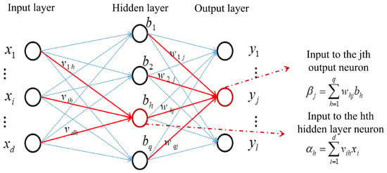
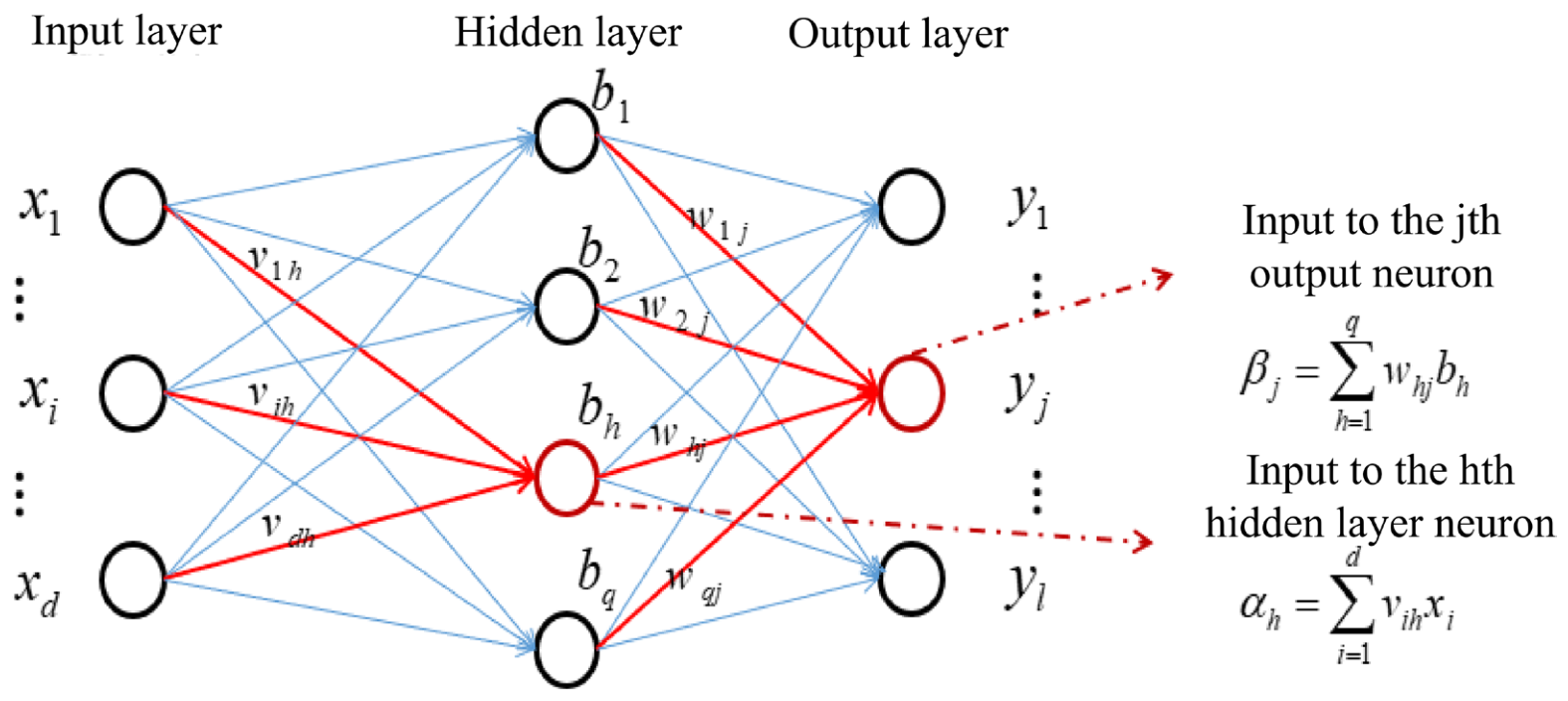
A backpropagation neural network (BPNN) is a feedforward neural network trained by error backpropagation [19,20]. In this study, it serves as a base nonlinear regression model for hydrate formation pressure. Figure 1 depicts the network architecture of the BPNN, which is a three-layer feedforward neural network composed of an input layer, a hidden layer, and an output layer.

Figure 1. Structure of the BPNN. Blue arrows indicate the network connections, and red arrows highlight the connections used to illustrate the calculations for the j-th output neuron and the h-th hidden neuron.

To determine the candidate range for the number of neurons in the hidden layer, this paper refers to the empirical formula used in existing research [21]:

$$J=\sqrt{m+n}+a$$

(5)

where $J$ represents the number of hidden layer neurons, and $m$ and $n$ represent the number of input-layer and output-layer nodes, respectively; $a$ is a constant ranging from 1 to 10. In this paper, $m=4$ and $n=1$ are used to set the number of candidate nodes to 3–12. This paper employs five random splits of the training data, performing five-fold cross-validation for each split, and uses the average validation set MAE as the comparison metric. The results for each number of nodes are shown in Table 1.

Table 1. Mean validation MAE for different numbers of BPNN hidden neurons.

Number of Nodes in the Hidden Layer	Average MAE (kPa)
3	698.33
4	644.41
5	785.8
6	704.92
7	603.71
8	618.87
9	581.96
10	694.57
11	609.68
12	749.44

As shown in Table 1, the configuration with 9 hidden layer neurons yields the lowest average validation set MAE. Thus, it is selected for the BPNN model.

In this paper, the BPNN network adopts a 4–9–1 architecture, meaning the input layer contains 4 nodes corresponding to temperature, methane content, ethane content, and propane content, respectively; the hidden layer contains 9 neurons; and the output layer contains 1 node corresponding to the hydrate formation pressure. The hidden layer and output layer use the tansig and purelin activation functions, respectively, and the network is trained using the Levenberg–Marquardt algorithm.

To avoid negative pressure predictions, the BPNN is trained to predict the natural logarithm of pressure, with pressure expressed in kPa. The predicted values are transformed back to kPa using the exponential function before evaluation.

2.2.2. Least-Squares Support Vector Regression Model

Least-squares support vector regression (LSSVR) formulates regression as a regularized squared-error optimization with equality constraints. The resulting optimality conditions form a linear system for estimating the model coefficients [22,23].

A kernel function allows LSSVR to represent nonlinear relationships [23,24]. In this study, linear, polynomial, and Gaussian kernels are compared using repeated five-fold cross-validation on the training data. For each of the 15 random seeds (1–15), the training data are shuffled and divided into five folds. Each fold is used once for validation, while the remaining four folds are used for training.

The regularization parameter of the linear kernel is searched over 0.001–500. For the polynomial kernel, the regularization parameter is searched over 0.001–500, the bias is set to 0 or 1, and the degree is set to 2 or 3. For the Gaussian kernel, the regularization parameter is searched over 0.001–500 and the kernel parameter over 0.001–100. Each parameter search uses 20 particles and 50 iterations.

The mean validation root mean square errors (RMSEs), averaged across the 15 repetitions and reported as the mean ± standard deviation, are 5401.47 ± 10.01, 689.17 ± 65.40, and 147.76 ± 1.27 kPa for the linear, polynomial, and Gaussian kernels, respectively. The Gaussian kernel achieves the lowest mean validation RMSE and is therefore selected.

For the Gaussian kernel LSSVR model, the regularization parameter controls the balance between the fitting error and the model complexity, while the kernel width parameter controls the smoothness of the nonlinear regression function. The optimization problem of LSSVR is written as:

$$\begin{array}{l}\underset{w,b,e_i}{\min }{\displaystyle \frac{1}{2}}{‖w‖}^2+{\displaystyle \frac{1}{2}}\lambda {\displaystyle {\sum }_{i=1}^m{e}_i^2}\\ s.t.f(x_i)-y_i=e_i,i=1,\dots ,m\end{array}$$

(6)

In this formulation, $e_i$ denotes the prediction residual, while $\lambda$ serves as the regularization parameter to govern the trade-off between the empirical risk and the structural complexity of the model. By introducing Lagrange multipliers and deriving the optimality conditions, the following system of equations is obtained:

$$\left\{\begin{array}{l}{\displaystyle \sum _{i=1}^m{\alpha }_i}k(x_i,x_j)+b+{\lambda }^{-1}{\alpha }_j=y_j,j=1,\dots ,m\\ {\displaystyle \sum _{i=1}^m{\alpha }_i=0}\end{array}\right.$$

(7)

By solving this linear system, the LSSVR regression function is obtained:

$$f\left(x\right)={\displaystyle \sum _{i=1}^m{\alpha }_i}k(x,x_i)+b$$

(8)

Unlike standard SVR, LSSVR replaces inequality constraints with equality constraints and obtains its solution from a linear system rather than an inequality-constrained quadratic program. The derivation still uses first-order optimality conditions.

2.3. Parameter Optimization Methods

The prediction performance of LSSVR is strongly affected by the regularization parameter and the Gaussian kernel parameter. To improve the rationality of parameter selection, particle swarm optimization and improved particle swarm optimization are used to search for suitable LSSVR parameters.

2.3.1. Particle Swarm Optimization

Particle swarm optimization (PSO) is a swarm-intelligence optimization algorithm inspired by the collaborative search and information-sharing behavior observed in group foraging [25]. In a D-dimensional target search space, a swarm consists of N particles, where each particle represents a candidate solution. The state of the $i$-th particle is characterized by its position vector $X_i$ and velocity vector $V_i$, which are defined as follows:

$$X_i=\left(x_{i1},x_{i2},\cdots x_{iD}\right),i=1,2,\cdots ,N$$

(9)

$$V_i=\left(v_{i1},v_{i2},\cdots v_{iD}\right),i=1,2,\cdots ,N$$

(10)

During the search process, each particle continuously adjusts its direction and velocity according to its historically best position and the historically best position of the swarm, gradually approaching the optimum of the objective function. Taking into account the particle’s own inertia, its individual optimal position, and the population’s optimal position, the formulas for updating the velocity and position of the $i$-th particle at the $t$-th iteration are as follows:

$$v_{ij}(t+1)=\omega v_{ij}(t)+c_1{r}_1(t)\lfloor p_{ij}(t)-x_{ij}(t)\rfloor +c_2{r}_2(t)\lfloor p_{gj}(t)-x_{ij}(t)\rfloor$$

(11)

$$x_{ij}(t+1)=x_{ij}(t)+v_{ij}(t+1)$$

(12)

Here, $\omega$ is the inertia weight, representing the particle’s ability to maintain its original motion state; $c_1$ and $c_2$ are the individual and global learning factors, respectively, used to adjust the extent to which the particle moves toward its individual best position $p_{ij}(t)$ and the global best position $p_{gj}(t)$; and $r_1(t)$ and $r_2(t)$ are random numbers between 0 and 1 used to increase the stochasticity of the particle search process.

The velocity update combines inertia, personal best information, global best information, and random factors [26].

2.3.2. Improved Particle Swarm Optimization

Although PSO has good global search capability during parameter optimization, it may still suffer from premature convergence and stagnation at local optima [26]. When the inertia weight and learning factors are fixed, particles adopt a relatively uniform search strategy throughout the iterations, making it difficult to balance global exploration in the early stage with local convergence in the later stage. To address these problems, this study combines two existing PSO modification strategies: a fitness-adaptive inertia weight $\omega$ and time-varying learning factors $c_1$ and $c_2$. This combination is referred to as improved particle swarm optimization (IPSO) in this study.

The inertia weight $\omega$ controls the extent to which a particle maintains its original motion state. The individual learning factor $c_1$ represents the weight assigned to the particle’s movement toward its historical best position, whereas the swarm learning factor $c_2$ represents the weight assigned to the particle’s movement toward the historical best position of the swarm. In the early iterations, the particles’ spatial search capability should be enhanced so that they can sufficiently explore different regions. In the later iterations, their ability to converge toward a better solution should be strengthened so that they gradually approach the global optimum.

Based on the fitness-adaptive inertia weight proposed by Liu et al. [27], the inertia weight is calculated as follows:

$$\omega =\left\{\begin{array}{l}{\omega }_{\min },f_{avg}=f_{\min }\\ {\omega }_{\min }+{\displaystyle \frac{\left({\omega }_{\max }-{\omega }_{\min }\right)\left(f-f_{\min }\right)}{f_{avg}-f_{\min }}},f_{avg}>f_{\min },f\le f_{avg}\\ {\omega }_{\max },f_{avg}>f_{\min },f>f_{avg}\end{array}\right.$$

(13)

Here, ${\omega }_{\min }$ and ${\omega }_{\max }$ are the preset minimum and maximum inertia weights, respectively; f is the fitness of the current particle; and f_min and f_avg are the minimum and average fitness values of all particles in the current iteration, respectively. When f_avg = f_min, ω is set to ω_min to avoid division by zero. For particles with fitness better than the average, a smaller ω reduces the influence of their previous velocity and promotes local search near the current favorable region. For particles with fitness worse than the average, ω_max promotes broader exploration.

The asymmetric adjustment formulas for $c_1$ and $c_2$ are given as follows [28]:

$$\begin{array}{l}{c}_1=c_1^{ini}+(c_1^{fin}-c_1^{ini})\ast {\displaystyle \frac{i}{M}}\\ c_2=c_2^{ini}+(c_2^{fin}-c_2^{ini})\ast {\displaystyle \frac{i}{M}}\end{array}$$

(14)

Here, the superscript $ini$ denotes the initial value, while $fin$ denotes the final value; both are initially specified parameters. $i$ represents the current iteration number, and $M$ represents the maximum number of iterations. It can be seen from the equations that, as the number of iterations increases, $c_1$ decreases linearly and $c_2$ increases linearly. This adjustment enables particles to rely more on individual historical experience during the early iterations and make greater use of the swarm’s global best information during the later iterations, thereby balancing global exploration and local convergence.

2.4. Evaluation Metrics

This study uses the mean absolute error (MAE), root mean square error (RMSE), mean absolute percentage error (MAPE), and coefficient of determination (R²) to evaluate model prediction performance. Before calculating MAE and RMSE, the predicted hydrate formation pressures are inverse-transformed to kPa using the output normalization parameters. These predictions are then compared with the reference pressures in kPa. Therefore, both MAE and RMSE are reported in kPa.

Let $n$ denote the number of test samples, $y_i$ the actual value, ${\widehat{y}}_i$ the predicted value, and $\overline{y}$ the mean actual value. The definitions of these metrics are given below.

MAE represents the mean absolute error between the predicted and actual values. It reflects the overall magnitude of the model prediction error, and its unit is the same as that of the predicted variable. Because the prediction target in this study is hydrate formation pressure, the unit of MAE is kPa:

$$MAE={\displaystyle \frac{1}{n}}{\displaystyle \sum _{i=1}^n\left|y_i-{\widehat{y}}_i\right|}$$

(15)

RMSE represents the square root of the mean squared prediction error. Because the errors are squared during calculation, RMSE is more sensitive to larger errors and can be used to reflect whether substantial deviations occur at individual sample points. The unit of RMSE is also kPa:

$$RMSE=\sqrt{{\displaystyle \frac{1}{n}}{\displaystyle \sum _{i=1}^n{\left(y_i-{\widehat{y}}_i\right)}^2}}$$

(16)

MAPE represents the mean absolute percentage error between the predicted and actual values. It is used to measure the magnitude of the prediction error relative to the actual value and is expressed as a percentage:

$$MAPE={\displaystyle \frac{100\%}{n}}{\displaystyle \sum _{i=1}^n\left|\frac{y_i-{\widehat{y}}_i}{y_i}\right|}$$

(17)

R² represents the proportion of variation in the actual values explained by the model and is used to evaluate the fitting performance between the predicted and actual values:

$$R^2=1-{\displaystyle \frac{{\displaystyle \sum _{i=1}^n{\left(y_i-{\widehat{y}}_i\right)}^2}}{{\displaystyle \sum _{i=1}^n{\left(y_i-\overline{y}\right)}^2}}}$$

(18)

When comparing the above metrics, lower MAE, RMSE, and MAPE values indicate lower prediction errors, whereas an R² value closer to 1 indicates better fitting performance for the test samples.

3. Case Study

3.1. Dataset Description and Preprocessing

The phase equilibrium pressures of natural gas hydrates used in this study are calculated by the CSMHYD program based on specified temperatures and gas compositions [29]. These are all calculated values and do not include experimentally measured values. Macelloni et al. [30] used the CSMHYD program to calculate the hydrate equilibrium conditions for the methane–ethane–propane system at different temperatures and gas compositions. Waage et al. [31] employed the CSMHYD program to calculate the stability boundaries of hydrates containing these three components. These studies provided a basis for selecting the CSMHYD program as the source of computational data in this paper.

Natural gas generally consists of multiple combustible and noncombustible gases, with methane as the major component and relatively smaller amounts of ethane, propane, and other light hydrocarbons. Considering common gas compositions in natural gas pipeline transportation, model complexity, and prediction accuracy, the gas composition is simplified in this study to three major components: methane, ethane, and propane. Temperature, methane content, ethane content, and propane content are used as input variables, and natural gas hydrate formation pressure is used as the output variable.

The training set is used to develop the models. Its temperature range is 253–303 K, with one temperature point selected every 2 K, giving 26 temperature points. Twenty-one gas composition combinations are specified, with methane content ranging from 90% to 100% and ethane and propane varying within the remaining fraction. Thus, each composition combination corresponds to 26 temperature points, producing 546 training samples. The composition combinations and corresponding numbers of data points are listed in Table 2.

Table 2. Training set natural gas component combinations and number of data points.

Natural Gas Components (%)			Number of Data Points
Methane Content	Ethane Content	Propane Content
100	0	0	26
98	2	0	26
98	0	2	26
96	4	0	26
96	2	2	26
96	0	4	26
94	6	0	26
94	4	2	26
94	2	4	26
94	0	6	26
92	8	0	26
92	6	2	26
92	4	4	26
92	2	6	26
92	0	8	26
90	10	0	26
90	8	2	26
90	6	4	26
90	4	6	26
90	2	8	26
90	0	10	26

The test set is used to evaluate model prediction performance. Its temperature range is 264–284 K, with one temperature point selected every 2 K, giving 11 temperature points. Methane content is set to five representative values: 91%, 93%, 95%, 97%, and 99%, while ethane and propane vary within the remaining fraction. The test set therefore contains 55 samples, as shown in Appendix A Table A1. Table 3 presents an example of the composition combinations for a methane content of 95%.

Table 3. Example of test set natural gas component combinations.

Temperature (K)	Natural Gas Components (%)
	Methane Content	Ethane Content	Propane Content
264	95	5	0
266	95	4.5	0.5
268	95	4	1
270	95	3.5	1.5
272	95	3	2
274	95	2.5	2.5
276	95	2	3
278	95	1.5	3.5
280	95	1	4
282	95	0.5	4.5
284	95	0	5

Because temperature, gas composition, and formation pressure have different units and numerical ranges, the input and output variables are normalized using the Min–Max Normalization method before modeling. This prevents differences in numerical scale from affecting model training and prediction results.

3.2. Grey Relational Analysis Results

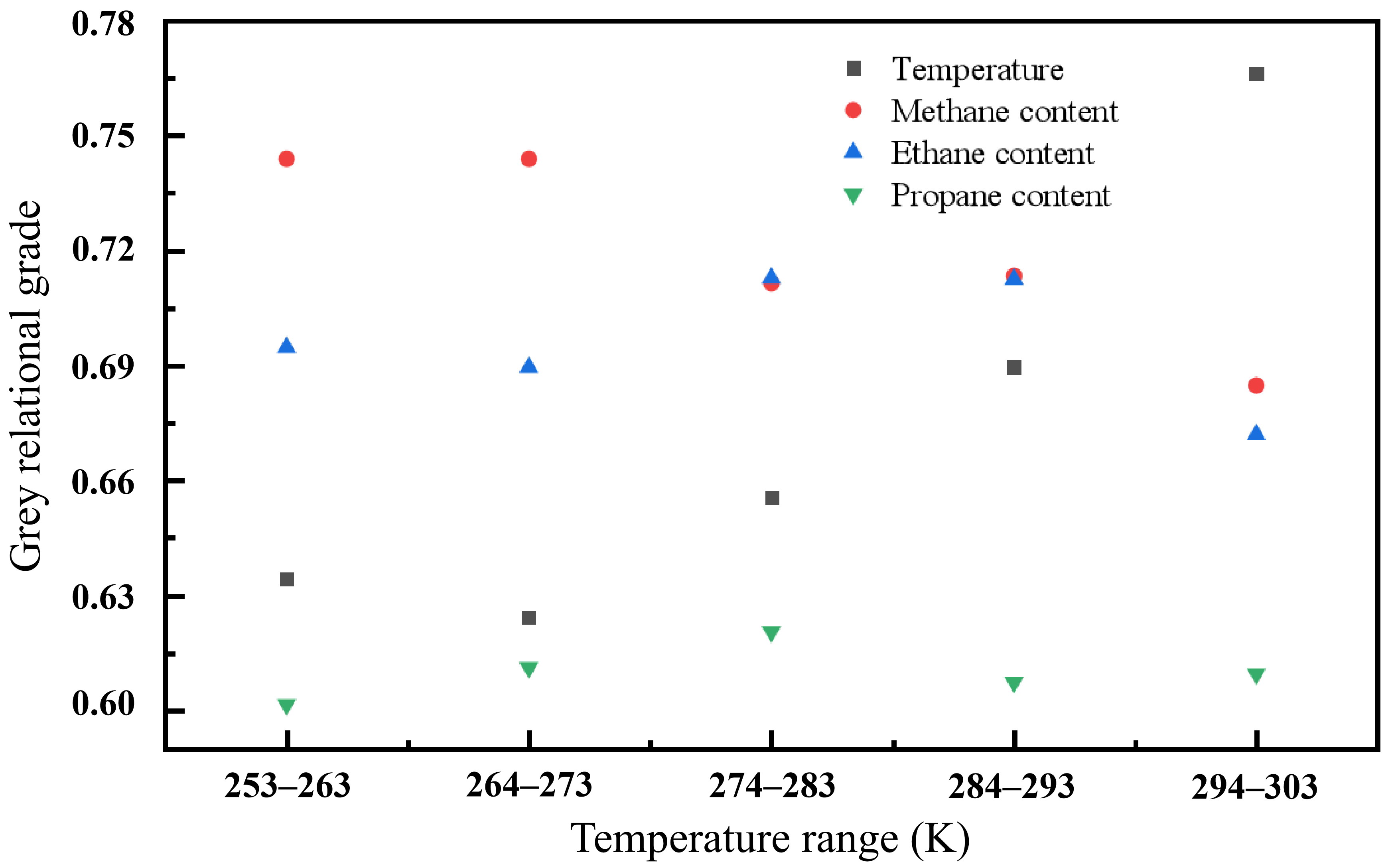
The grey relational grades between the input variables and natural gas hydrate formation pressure are compared across temperature intervals. Considering the temperature dependence of gas thermodynamic properties and hydrate phase equilibrium, the training samples are divided into five intervals: 253–263 K, 264–273 K, 274–283 K, 284–293 K, and 294–303 K. Table 4 presents the grey relational grades for temperature, methane content, ethane content, and propane content in each interval.

Table 4. Grey relational grades between input variables and formation pressure in different temperature intervals.

Temperature Range	Grey Relational Grade
	Temperature	Methane	Ethane	Propane
253 K~263 K	0.6344	0.7439	0.6947	0.6015
264 K~273 K	0.6244	0.7439	0.6895	0.6111
274 K~283 K	0.6556	0.7115	0.7128	0.6205
284 K~293 K	0.6896	0.7134	0.7125	0.6073
294 K~303 K	0.7663	0.6848	0.6720	0.6095

As shown in Table 4, the rankings vary across intervals. At 253–263 K and 264–273 K, methane content has the highest grade among the four variables, at 0.7439 in both intervals. At 274–283 K, the grade for ethane content (0.7128) is slightly higher than that for methane content (0.7115). At 284–293 K, their grades are close, at 0.7125 and 0.7134, respectively. At 294–303 K, temperature has the highest grade, at 0.7663. Because the grades do not show a clear separation among the four variables and the rankings vary across temperature intervals, these results do not provide a clear basis for excluding any one variable. Therefore, all four variables are retained as inputs to the subsequent prediction models. Notably, because the input conditions were generated on a regular grid, the grades may partly reflect the sampling design and should be interpreted only in the context of the dataset analyzed here.

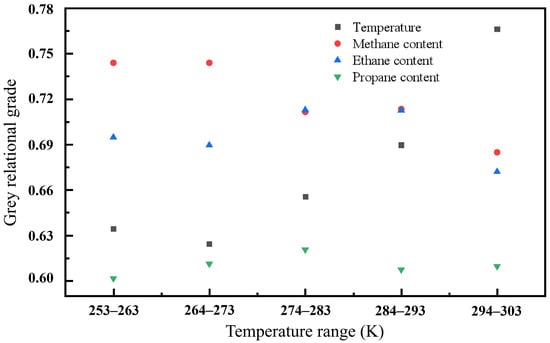
Figure 2 further illustrates how the grades vary across temperature intervals. The grade for temperature generally increases, whereas that for methane content generally decreases. Ethane content has a relatively high grade in the intermediate-temperature intervals, while propane content has relatively low grades throughout. Methane, ethane, and propane contents sum to 100% and are therefore not independent. These grades describe the similarity between each input variable sequence and the pressure sequence; they do not establish the independent effect of any component or a causal relationship.

Figure 2. Comparison of grey relational grades among input variables.

3.3. Base Model Prediction

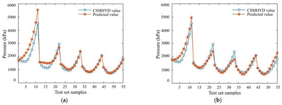
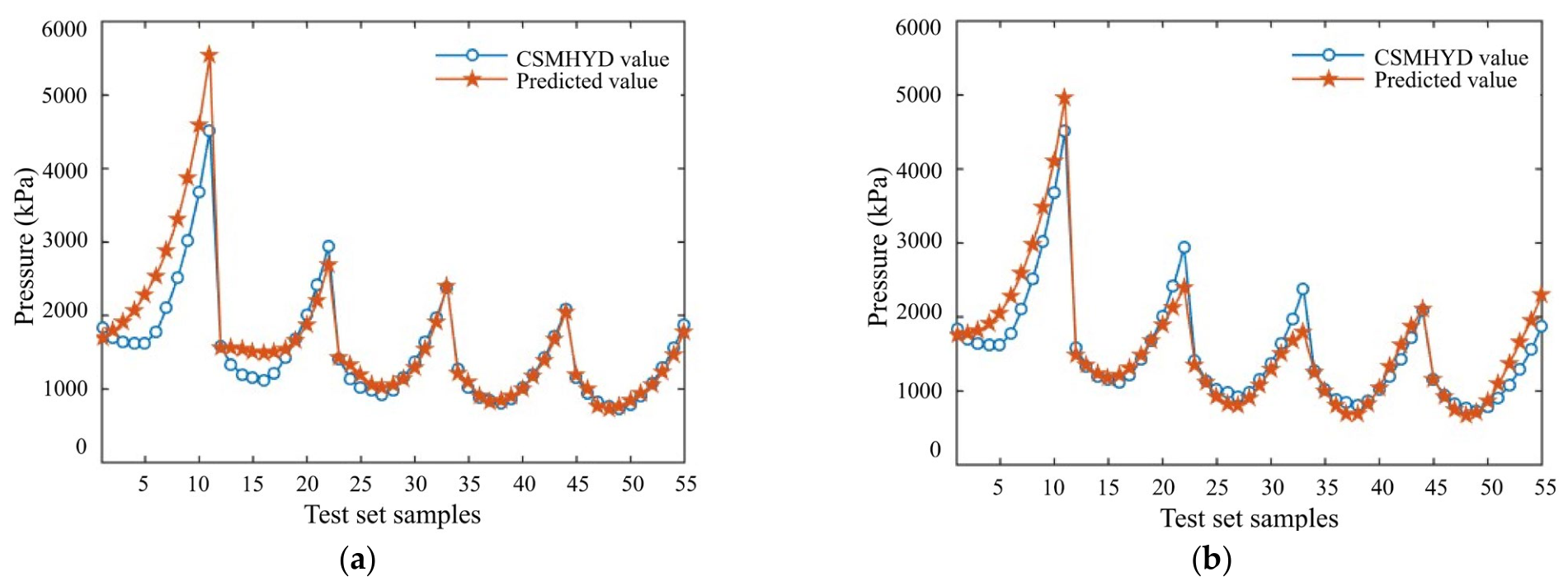
A BPNN and an LSSVR base regression model are established to predict natural gas hydrate formation pressure in the test set. Figure 3 compares the predicted and actual values of the two models. The horizontal axis represents the test sample index, and the vertical axis represents hydrate formation pressure.

Figure 3. Comparison between predicted and actual hydrate formation pressure obtained by basic regression models. (a) Prediction results of the BPNN model; (b) prediction results of the LSSVR model.

Figure 3 shows that both BPNN and LSSVR capture the overall variation trend of hydrate formation pressure in the test samples, indicating that both base regression models can describe the nonlinear relationship between the input variables and formation pressure. However, the BPNN shows noticeable deviations at some sample points. In contrast, the LSSVR predictions are generally closer to the actual values, with better curve agreement at most sample points, indicating lower prediction error on this dataset.

Table 5 lists the evaluation results for the BPNN and LSSVR models on the test set. For the LSSVR model, this study employs a Gaussian radial basis function kernel and determines the regularization and kernel parameters through five-fold cross-validation on the training set. The search ranges for these parameters are 0.001–500 and 0.001–100, respectively, and the final selected values are 344.61 and 0.2015. After determining the parameters, the model is refit using the complete training set, and its performance is evaluated on the test set.

Table 5. Test set prediction error metrics for the BPNN and baseline LSSVR models.

Model	MAE (kPa)	RMSE (kPa)	MAPE (%)	R2
BPNN	200	330	11.34	0.7984
LSSVR	179	246	11	0.8883

As shown in Table 5, the BPNN has MAE, RMSE, MAPE, and R² values of 200 kPa, 330 kPa, 11.34%, and 0.7984, respectively, whereas the corresponding LSSVR values are 179 kPa, 246 kPa, 11.0%, and 0.8883. Overall, compared with the BPNN, the LSSVR exhibits smaller prediction errors and better fitting performance on the test set. Therefore, LSSVR is used as the base model in the subsequent analysis to examine the effect of parameter optimization on prediction results.

3.4. Prediction with Optimized LSSVR Models

LSSVR prediction performance is strongly affected by the regularization parameter and the Gaussian kernel parameter, and their values directly influence prediction accuracy and stability. To improve the selection of LSSVR parameters, PSO and IPSO are used to search for suitable parameter combinations, and PSO-LSSVR and IPSO-LSSVR models are established. During parameter optimization, fitness is defined as the mean validation RMSE obtained from five-fold cross-validation on the training data. For each candidate parameter combination, the model is trained on four folds and evaluated on the remaining fold, and the RMSE values from the five validation folds are averaged. A lower fitness value indicates a lower mean validation error. The same fixed five-fold partition is used to evaluate every candidate parameter combination.

Both PSO-LSSVR and IPSO-LSSVR use a Gaussian kernel and search for the LSSVR regularization parameter and the Gaussian kernel parameter. The two optimized models use the same basic settings: a swarm size of 20, a maximum of 50 iterations, a regularization parameter search range of 0.001–500, a Gaussian kernel parameter search range of 0.001–100, and a maximum particle velocity of 6. Previous studies have also used similar parameter ranges: Li et al. [32] set the regularization parameter to 0.001–500; Xu et al. [33] set the search range for the Gaussian kernel parameter to 0.01–100.

To investigate the impact of the search bounds, this paper expands the upper bounds for the regularization parameter and Gaussian kernel parameter to 1000 and 200, respectively, and runs the optimization program using three random seeds; the results are shown in Table 6.

Table 6. Results of the simulation after expanding the upper bound of the search.

Random Seed	Optimal Regularization Parameter	Optimal Gaussian Kernel Parameter	RMSE (kPa)
1	417.22	0.2031	147.31
2	235.16	0.1534	158.29
3	400.04	0.2011	147.65

As shown in Table 6, the parameters obtained from the three random runs all fall within the original search range. This indicates that, in these three runs, expanding the search region does not alter the range within which the parameters are found.

In PSO, the inertia weight decreases linearly from 0.9 to 0.6, and both the individual and global learning factors are 2. In IPSO, the inertia weight is adjusted according to particle fitness within the range of 0.6–0.9; the individual learning factor decreases from 2.5 to 0.5, and the global learning factor increases from 0.5 to 2.5. The selected values of the regularization parameter and Gaussian kernel parameter are 425.96 and 0.20 for PSO-LSSVR, and 470.52 and 0.21 for IPSO-LSSVR, respectively.

Accounting for the stochasticity of PSO and IPSO, both optimization algorithms were run 15 times using random seeds 2026–2030, 2036–2040, and 2046–2050. The same training and test sets were used in every run. Table 7 reports the mean and standard deviation of the test set metrics across these runs. Because the baseline LSSVR uses fixed parameters, its metrics are reported from a single run.

Table 7. Prediction error metrics for the LSSVR, PSO-LSSVR, and IPSO-LSSVR.

Model	MAE (kPa)	RMSE (kPa)	MAPE (%)	R2
LSSVR	179	246	11	0.8883
PSO-LSSVR	108.235 ± 0.475	147.751 ± 1.143	6.710 ± 0.024	0.9597 ± 0.0006
IPSO-LSSVR	107.921 ± 0.263	146.904 ± 0.847	6.695 ± 0.019	0.9602 ± 0.0005

As shown in Table 7, both optimized models reduce the prediction errors compared with the baseline LSSVR. Across the 15 runs, IPSO-LSSVR has slightly lower mean MAE, RMSE, and MAPE and a slightly higher mean R² than PSO-LSSVR. The differences are modest, indicating a small average improvement with IPSO-LSSVR.

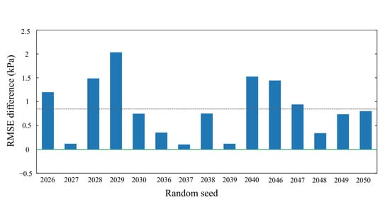
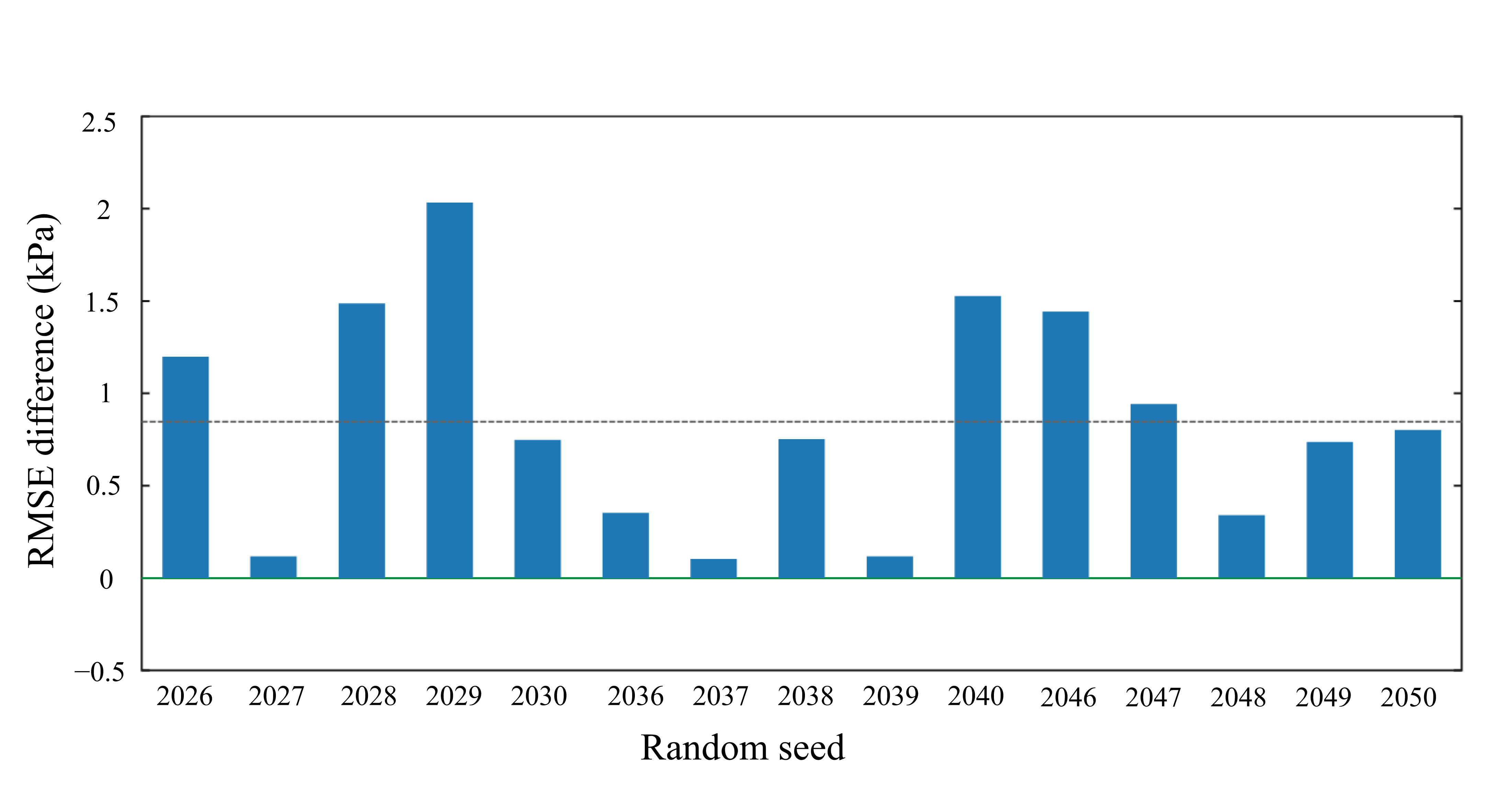
To visualize the results in Table 7 more directly, Figure 4 shows the test set RMSE difference between PSO-LSSVR and IPSO-LSSVR for each of the 15 runs. The zero line represents equal RMSE, and the dashed line indicates the mean difference of 0.847 kPa.

Figure 4. Run-wise differences in the test set RMSE between PSO-LSSVR and IPSO-LSSVR.

As shown in Figure 4, the RMSE differences vary across runs but are generally small. Overall, IPSO-LSSVR achieves a slightly lower test set RMSE than PSO-LSSVR.

To investigate the impact of noisy inputs on predictions, the IPSO-LSSVR model remains unchanged, and simulated perturbations are applied to the test samples. Zero-mean Gaussian noise is added to the temperature, ethane content, and propane content of each test sample, respectively. The standard deviations of the temperature noise are set to 0.05, 0.10, and 0.15 K, respectively; the standard deviations of the ethane and propane content noise are set to 0.05, 0.10, and 0.15 mole percent, respectively. After perturbation, the components are adjusted to ensure they are non-negative and sum to 100%. The evaluation is repeated 100 times for each noise level; the results are shown in Table 8.

Table 8. IPSO-LSSVR prediction results at different noise levels.

Standard Deviation of Temperature/Composition Noise (K/mol%)	MAE (kPa)	RMSE (kPa)	MAPE (%)	R2
0.05/0.05	108.49 ± 4.84	150.43 ± 10.17	6.73 ± 0.25	0.9580 ± 0.0057
0.10/0.10	112.28 ± 9.09	162.35 ± 20.09	6.98 ± 0.45	0.9506 ± 0.0123
0.15/0.15	119.37 ± 12.91	179.65 ± 29.65	7.44 ± 0.63	0.9388 ± 0.0209

As shown in Table 8, as the noise level increases, the average prediction error and its variability also increase. However, the model still maintains a certain level of predictive capability across the three noise levels tested, indicating that IPSO-LSSVR exhibits a certain degree of tolerance to the simulated input noise used in this study.

Table 9 provides a further run-level assessment of PSO-LSSVR and IPSO-LSSVR. It reports the random seed, selected regularization parameter, Gaussian kernel parameter, and corresponding test set RMSE for each run.

Table 9. Run-level optimal parameters and test set RMSEs for PSO-LSSVR and IPSO-LSSVR.

Random Seed	Optimal Regularization Parameter		Optimal Gaussian Radial Basis Kernel Square		RMSE (kPa)
	PSO- LSSVR	IPSO- LSSVR	PSO- LSSVR	IPSO- LSSVR	PSO- LSSVR	IPSO- LSSVR
1	326.76	365.94	0.1971	0.1999	149.29	148.34
2	319.31	438.13	0.1968	0.2094	149.49	146.90
3	306.44	441.85	0.1981	0.2069	149.85	146.85
4	407.63	500.00	0.2074	0.2137	147.46	145.93
16	356.12	406.24	0.2016	0.2072	148.55	147.48
17	380.59	446.76	0.2051	0.209	148	146.75
18	405.09	444.83	0.2096	0.2112	147.53	146.79
19	424.22	449.83	0.2041	0.2082	147.17	146.71
20	429.51	451.32	0.2113	0.2125	147.07	146.69
21	423.16	432.93	0.2092	0.2087	147.17	146.99
22	469.73	492.48	0.2115	0.2143	146.38	146.04
23	386.29	456.65	0.2019	0.2133	147.9	146.6
24	379.97	456.91	0.2073	0.21	148.04	146.59

As shown in Table 9, in the 13 runs, the average RMSE of IPSO-LSSVR is slightly lower than that of PSO-LSSVR. In the fourth IPSO-LSSVR run, the regularization parameter reaches the upper limit of 500.00. To verify this, this paper repeats the run while maintaining the same random seed and other optimization settings, and sets the upper limit of the regularization parameter to 650, 800, and 950, respectively. The resulting regularization parameter remains at 500.00.

To more comprehensively evaluate the method proposed in this paper, this study compares representative machine-learning methods used in the relevant literature [13,14,15,16,17], including adaptive neural-fuzzy inference systems, multi-layer perceptrons, deep multi-layer perceptrons, random forests, and GWO-LSSVM. Additionally, common support vector regression methods and the Klauda–Sandler thermodynamic model implemented by the P2F Hydrate Calculator [34] are included. Table 10 shows the prediction results of each method compared to those of IPSO-LSSVR. The parameter search ranges and selected settings corresponding to the results in Table 10 are summarized in Appendix A Table A2.

Table 10. Prediction results of different models.

Model	MAPE (%)
P2F (Klauda–Sandler model)	8.32
Adaptive neuro-fuzzy inference model	13.10
Multi-layer perceptron neural network	24.80
Deep multi-layer perceptron model	25.65
RF	22.13
GWO-LSSVM	6.67
SVR	14.85
IPSO-LSSVR	6.63

As shown in Table 10, among the machine-learning models, the MAPE value of IPSO-LSSVR is lower than that of other methods and differs only slightly from the MAPE value of GWO-LSSVM. The P2F value in Table 10 represents the difference between two thermodynamic programs and is not included in this comparison.

To examine the model’s predictive performance near the boundaries of the training range, this study establishes four sets of new CSMHYD calculation conditions. To examine the temperature boundary and the methane content boundary separately, when one variable approaches a boundary, the other variable is kept within the training range to prevent both from approaching their respective boundaries simultaneously. Ten samples are randomly selected from each set of generated operating conditions, and the IPSO-LSSVR model with fixed parameters is evaluated using the CSMHYD-calculated pressure as a reference value. The results are shown in Table 11. For each new condition, temperature and methane content were sampled independently within the specified group ranges; ethane and propane were randomly allocated from the remaining mole fraction so that the three components summed to 100%.

Table 11. Prediction results of IPSO-LSSVR near the boundaries of the training range.

Boundary Condition Groups	Temperature (K)	Methane Content (mol%)	MAPE (%)
Near the lower temperature limit	253–255	91–99	15.77
Near the upper temperature limit	301–303	91–99	2.10
Near the lower methane content limit	255–301	90–91	6.82
Near the upper methane content limit	255–301	99–100	10.22

As shown in Table 11, there are differences in the MAPE across the four sets of operating conditions. The IPSO-LSSVR model exhibits varying degrees of agreement with the CSMHYD-calculated values near the boundaries of the training range; in particular, the relative error is relatively large near the lower temperature limit.

To examine the model’s performance outside the training range, this study adds operating conditions where the temperature or methane content exceeds the training range. Ten samples are randomly selected from each set of operating conditions, and the pressure calculated using CSMHYD is used as a reference value to evaluate the IPSO-LSSVR model with fixed parameters. The results are shown in Table 12.

Table 12. Prediction results of IPSO-LSSVR under out-of-training-range conditions.

Out-of-Range Condition Group	Temperature (K)	Methane Content (mol%)	MAPE (%)
Outside the temperature range	245–252 or 304–311	91–99	6.11
Outside the methane content range	255–301	85–89	9.80

As shown in Table 12, the IPSO-LSSVR model exhibits differences in error across the temperature and methane concentration out-of-range categories, with larger errors when extrapolating in the direction of methane concentration exceeding the range than when extrapolating in the direction of temperature exceeding the range. These boundary and out-of-range assessments are diagnostic evaluations against CSMHYD-calculated pressures; they do not replace independent experimental or field validation.

For individual calculations, CSMHYD can be used directly. The potential utility of the trained surrogate is convenient approximate evaluation of repeated or batch queries within the studied domain. This convenience comes with an approximation error. Where closer agreement with the thermodynamic calculation is needed, direct use of CSMHYD remains preferable.

4. Conclusions

This study develops a machine-learning method for approximating CSMHYD-calculated hydrate formation pressures. The main conclusions are as follows:

(1)

The grey relational grades of temperature, methane content, ethane content, and propane content vary across temperature intervals. Methane content has the highest grade in the 253–263 K and 264–273 K intervals, at 0.7439 in both. Ethane content has the highest grade in the 274–283 K interval, at 0.7128, whereas temperature has the highest grade in the 294–303 K interval, at 0.7663.

(2)

The BPNN has MAE, RMSE, MAPE, and R² values of 200 kPa, 330 kPa, 11.34%, and 0.7984, respectively, while the corresponding LSSVR values are 179 kPa, 246 kPa, 11.0%, and 0.8883. LSSVR therefore provides lower prediction error and better fitting performance.

(3)

Across 15 runs, PSO-LSSVR has mean MAE, RMSE, MAPE, and R2 values of 108.235 ± 0.475 kPa, 147.751 ± 1.143 kPa, 6.710 ± 0.024%, and 0.9597 ± 0.0006, respectively. The corresponding IPSO-LSSVR means are 107.921 ± 0.263 kPa, 146.904 ± 0.847 kPa, 6.695 ± 0.019%, and 0.9602 ± 0.0005. The results indicate a modest average improvement with IPSO-LSSVR over PSO-LSSVR.

The main limitations of this study are as follows:

(1)

Among the models compared in this study, IPSO-LSSVR achieves the lowest MAPE relative to the CSMHYD-calculated pressures. Because the models are trained and evaluated using pressures calculated by CSMHYD, the reported errors measure agreement with that program, not accuracy against experimentally measured hydrate formation pressures. Generating an experimental dataset covering the full temperature and composition ranges studied here would require substantial time and resources. Consequently, no independent experimental validation is conducted.

(2)

The training data comprise regular combinations of temperature and gas composition, and the original test samples fall within the range covered by the training data. Actual pipeline operating conditions may have a more irregular distribution. However, field data that simultaneously record temperature, gas composition, and reliable hydrate formation observations are difficult to obtain, and independent field validation is currently lacking. Therefore, the existing results do not establish the models’ predictive performance under irregular field conditions.

(3)

The models were developed only for methane–ethane–propane mixtures within the temperature range studied here and do not account for CO₂, N₂, H₂S, heavier hydrocarbons, or hydrate inhibitors. Therefore, conclusions concerning pipeline application are limited to the three-component system, conditions, and models tested in this study. Broader practical conclusions require validation using independent data for natural gas mixtures with more complex compositions.

The corresponding future research directions are as follows:

(1)

Collect independent experimental hydrate phase equilibrium pressure data to evaluate prediction errors against measured pressures and assess model performance beyond reproducing CSMHYD calculations.

(2)

Collect field data with reliable operating-condition and hydrate formation records to assess how field conditions differ from the regular grid data used here and to evaluate the models under actual pipeline conditions.

(3)

Expand the dataset to include other gas components, inhibitors, and a broader range of operating conditions. Retrain and validate the models using independent data for these more complex mixtures to establish their revised applicability limits.

References

- Sloan, E.D.; Koh, C.A. Clathrate Hydrates of Natural Gases, 3rd ed.; CRC Press: Boca Raton, FL, USA, 2007. [Google Scholar]
- Carroll, J. Natural Gas Hydrates: A Guide for Engineers, 2nd ed.; Gulf Professional Publishing: Oxford, UK, 2009. [Google Scholar]
- Sloan, E.D. Fundamental principles and applications of natural gas hydrates. Nature 2003, 426, 353–359. [Google Scholar] [CrossRef] [Scilit] [PubMed]
- Wilcox, W.I.; Carson, D.B.; Katz, D.L. Natural gas hydrates. Ind. Eng. Chem. 1941, 33, 662–665. [Google Scholar] [CrossRef] [Scilit]
- Parrish, W.R.; Prausnitz, J.M. Dissociation pressures of gas hydrates formed by gas mixtures. Ind. Eng. Chem. Process Des. Dev. 1972, 11, 26–35. [Google Scholar] [CrossRef] [Scilit]
- Adisasmito, S.; Frank, R.J.; Sloan, E.D. Hydrates of carbon dioxide and methane mixtures. J. Chem. Eng. Data 1991, 36, 68–71. [Google Scholar] [CrossRef] [Scilit]
- Adisasmito, S.; Sloan, E.D. Hydrates of hydrocarbon gases containing carbon dioxide. J. Chem. Eng. Data 1992, 37, 343–349. [Google Scholar] [CrossRef] [Scilit]
- Song, K.Y.; Kobayashi, R. Measurement and interpretation of the water content of a methane–propane mixture in the gaseous state in equilibrium with hydrate. Ind. Eng. Chem. Fundam. 1982, 21, 391–395. [Google Scholar] [CrossRef] [Scilit]
- Ng, H.-J.; Robinson, D.B. Hydrate formation in systems containing methane, ethane, propane, carbon dioxide or hydrogen sulfide in the presence of methanol. Fluid Phase Equilib. 1985, 21, 145–155. [Google Scholar] [CrossRef] [Scilit]
- Zahedi, G.; Karami, Z.; Yaghoobi, H. Prediction of hydrate formation temperature by both statistical models and artificial neural network approaches. Energy Convers. Manag. 2009, 50, 2052–2059. [Google Scholar] [CrossRef] [Scilit]
- Soroush, E.; Mesbah, M.; Shokrollahi, A.; Rozyn, J.; Lee, M.; Kashiwao, T.; Bahadori, A. Evolving a robust modeling tool for prediction of natural gas hydrate formation conditions. J. Unconv. Oil Gas Resour. 2015, 12, 45–55. [Google Scholar] [CrossRef] [Scilit]
- Ghavipour, M.; Ghavipour, M.; Chitsazan, M.; Najibi, S.H.; Ghidary, S.S. Experimental study of natural gas hydrates and a novel use of neural network to predict hydrate formation conditions. Chem. Eng. Res. Des. 2013, 91, 264–273. [Google Scholar] [CrossRef] [Scilit]
- Zeinali, N.; Ameri, A.; Saber, M. Comparative analysis of hydrate formation pressure applying cubic equations of state, artificial neural network and adaptive neuro-fuzzy inference system. Int. J. Thermodyn. 2012, 15, 91–101. [Google Scholar] [CrossRef] [Scilit][Green Version]
- Babakhani, S.M.; Bahmani, M.; Shariati, J.; Badr, K.; Balouchi, Y. Comparing the capability of artificial neural network and CSMHYD program for predicting hydrate formation pressure in binary mixtures. J. Pet. Sci. Eng. 2015, 136, 78–87. [Google Scholar] [CrossRef] [Scilit]
- Landgrebe, M.K.B.; Nkazi, D. Toward a Robust, Universal Predictor of Gas Hydrate Equilibria by Means of a Deep Learning Regression. ACS Omega 2019, 4, 22399–22417. [Google Scholar] [CrossRef] [Scilit] [PubMed]
- Yu, Z.; Tian, H. Application of Machine Learning in Predicting Formation Condition of Multi-Gas Hydrate. Energies 2022, 15, 4719. [Google Scholar] [CrossRef] [Scilit]
- Song, Y.-L.; Guo, P.; Liu, H.; Sun, B.-W. Application of Four Intelligent Models for the Estimation of Formation Pressure of Natural Gas Hydrate. Chem. Eng. Res. Des. 2024, 207, 281–294. [Google Scholar] [CrossRef] [Scilit]
- Deng, J.-L. Control problems of grey systems. Syst. Control Lett. 1982, 1, 288–294. [Google Scholar] [CrossRef] [Scilit]
- Bai, H.; Feng, T.; Du, K.; Shi, L.; Xin, C.; Mi, N. Gas Well Production Allocation Method Based on BP Neural Network. China Sci. 2023, 18, 1000–1006. [Google Scholar]
- Rumelhart, D.E.; Hinton, G.E.; Williams, R.J. Learning representations by back-propagating errors. Nature 1986, 323, 533–536. [Google Scholar] [CrossRef] [Scilit]
- Fan, X.-H.; Li, Y.; Chen, X.-L. Prediction of Iron Ore Sintering Characters on the Basis of Regression Analysis and Artificial Neural Network. Energy Procedia 2012, 16, 769–776. [Google Scholar] [CrossRef] [Scilit]
- Smola, A.J.; Schölkopf, B. A tutorial on support vector regression. Stat. Comput. 2004, 14, 199–222. [Google Scholar] [CrossRef] [Scilit]
- Suykens, J.A.K.; Van Gestel, T.; De Brabanter, J.; De Moor, B.; Vandewalle, J. Least Squares Support Vector Machines; World Scientific: Singapore, 2002. [Google Scholar]
- Schölkopf, B.; Smola, A.J. Learning with Kernels: Support Vector Machines, Regularization, Optimization, and Beyond; MIT Press: Cambridge, MA, USA, 2002. [Google Scholar]
- Kennedy, J.; Eberhart, R. Particle swarm optimization. In Proceedings of the IEEE International Conference on Neural Networks, Perth, Australia, 27 November–1 December 1995; IEEE: Piscataway, NJ, USA, 1995; Volume 4, pp. 1942–1948. [Google Scholar] [CrossRef] [Scilit]
- Shi, Y.; Eberhart, R.C. A modified particle swarm optimizer. In Proceedings of the IEEE International Conference on Evolutionary Computation, Anchorage, AK, USA, 4–9 May 1998; IEEE: Piscataway, NJ, USA, 1998; pp. 69–73. [Google Scholar] [CrossRef] [Scilit]
- Liu, B.; Wang, L.; Jin, Y.-H.; Tang, F.; Huang, D.-X. Improved particle swarm optimization combined with chaos. Chaos Solitons Fractals 2005, 25, 1261–1271. [Google Scholar] [CrossRef] [Scilit]
- Ratnaweera, A.; Halgamuge, S.K.; Watson, H.C. Self-organizing hierarchical particle swarm optimizer with time-varying acceleration coefficients. IEEE Trans. Evol. Comput. 2004, 8, 240–255. [Google Scholar] [CrossRef] [Scilit]
- Sloan, E.D. The Colorado School of Mines Hydrate Prediction Program (CSMHYD); Center for Hydrate Research, Colorado School of Mines: Golden, CO, USA, 1996. [Google Scholar]
- Macelloni, L.; Lutken, C.B.; Garg, S.; Simonetti, A.; D’EMidio, M.; Wilson, R.; Sleeper, K.; Lapham, L.; Lewis, T.; Pizzi, M.; et al. Heat-flow regimes and the hydrate stability zone of a transient, thermogenic, fault-controlled hydrate system (Woolsey Mound, northern Gulf of Mexico). Mar. Pet. Geol. 2015, 59, 491–504. [Google Scholar] [CrossRef] [Scilit]
- Waage, M.; Portnov, A.; Serov, P.; Bünz, S.; Waghorn, K.A.; Vadakkepuliyambatta, S.; Mienert, J.; Andreassen, K. Geological Controls on Fluid Flow and Gas Hydrate Pingo Development on the Barents Sea Margin. Geochem. Geophys. Geosystems 2019, 20, 630–650. [Google Scholar] [CrossRef] [Scilit]
- Li, H.; Su, Y.; Li, Z.; Zhang, Y. Foundation Pit Soil Parameter Inversion and Deformation Prediction Based on ESFOA and Hybrid Kernel LSSVM. Appl. Sci. 2026, 16, 2247. [Google Scholar] [CrossRef] [Scilit]
- Xu, Y.; Cheng, Z.; He, G.; Liang, C. Temperature Compensation for Semiconductor Gas Sensors Based on Whale Optimization Algorithm–Least-Squares Support Vector Machine. Sens. Mater. 2023, 35, 2933–2946. [Google Scholar] [CrossRef] [Scilit]
- Kunneman, K.; Sum, A.K. p2f-hydratecalc: A web Python-based tool for the prediction of natural gas hydrate equilibrium and inhibition. SoftwareX 2025, 32, 102422. [Google Scholar] [CrossRef] [Scilit]
Disclaimer/Publisher’s Note: The statements, opinions and data contained in all publications are solely those of the individual author(s) and contributor(s) and not of MDPI and/or the editor(s). MDPI and/or the editor(s) disclaim responsibility for any injury to people or property resulting from any ideas, methods, instructions or products referred to in the content. |
© 2026 by the authors. Licensee MDPI, Basel, Switzerland. This article is an open access article distributed under the terms and conditions of the Creative Commons Attribution (CC BY) license.