Research on Sensor Layout Strategy Based on Inverse Finite Element Deformation Reconstruction Using an Enhanced NSGA-III Algorithm

Abstract

Strain sensor placement strongly influences the accuracy and cost of deformation reconstruction with the inverse finite element method (iFEM). This study develops a common sensor layout for several loading regimes by coupling the four-node inverse shell element with a Lichtenberg-inspired local search embedded in the Non-dominated Sorting Genetic Algorithm III (LA-NSGA-III). At a prescribed sensor count, the layout is optimized by simultaneously minimizing reconstruction residuals for multiple training loads. The method is assessed using DTLZ benchmarks and a plate example under equal objective-evaluation budgets, with separate controls for the multi-load formulation and the local search operator. Across 20 paired plate runs with 23 sensor sites, the proposed search reduces the mean joint training residual by 18.65% relative to NSGA-III, with mean displacement errors of 0.73% and 0.77% for the two training loads. Additional pressure, torsional and off-center force cases, a withheld combined load, strain noise, and sensor loss are used to assess a fixed layout under changing conditions. A cantilever plate test demonstrates strain-based displacement reconstruction, with laser peak displacement measurements used to calibrate the FE reference model. The method supports the offline design of a single sensor layout for iFEM reconstruction under multiple anticipated loading conditions, reducing the need to reposition sensors when the load changes.

1. Introduction

In modern society, with the continuous development of industrial technology, engineering structures are becoming larger and more intelligent. Technologies for intelligent monitoring and operation–maintenance [1,2,3] have become a crucial component in ensuring the long-term health and functionality of such structures. For various structural health monitoring (SHM) systems, the core objective is to achieve real-time deformation assessment or vibration monitoring using data collected from various sensors. Therefore, various sensors, including accelerometers, displacement sensors, and strain gauges, are widely used in structural health monitoring applications.

The inverse finite element method (iFEM), first proposed by Tessler and his colleagues [4], reconstructs displacement fields from measured strains through a least squares variational formulation. It does not require the applied loads or material constitutive properties during reconstruction [5,6,7] and has been applied to aerospace, marine, and mechanical structures [8,9,10].

The above research has demonstrated the effectiveness and broad applicability of the iFEM. However, to achieve accurate reconstruction using iFEM, a large number of sensors need to be used and precisely placed. In practical applications, it is necessary to optimize the arrangement of sensors to improve deformation reconstruction, while reducing the number of sensors used to achieve cost reduction. Researchers have already conducted some studies on sensor placement in iFEM. For example, M. Ghasemzadeh and A. Kefal [11] combined a genetic algorithm (GA) [12] with a four-node quadrilateral element algorithm to optimize sensor placement for plate and shell structures. X. Li et al. [13] employed a multi-objective particle swarm optimization algorithm to optimize sensor placement for beam deformation reconstruction. Roy et al. [14] conducted a series of exploratory studies on sensor placement strategies for rectangular plates. The sensor optimization arrangements made by previous researchers were only targeted at a certain load form. However, in practical engineering, the structure is subjected to very complex loads, and the working conditions cannot guarantee that the entire structure will always be subjected to only one load form. Using the sensor optimization arrangement scheme optimized for a single load under different load conditions may lead to distortion of the deformation contour plots or significant errors in deformation values.

This study addresses two related questions: how does including several load responses change a sensor layout, and how does a Lichtenberg-inspired search [15] change the performance of NSGA-III [16] for the same placement problem? The first is tested by comparing single-load and multi-load objectives with the same genetic algorithm (GA); the second is tested by comparing LA-NSGA-III, NSGA-III, and NSGA-II under identical multi-load objectives and evaluation budgets. The numerical assessment uses two mirror-symmetric loads to examine transfer between load locations, followed by three distinct training load distributions and a withheld combined load to evaluate reconstruction under different loading regimes.

2. Methodology

2.1. iFEM-iQS4 Element

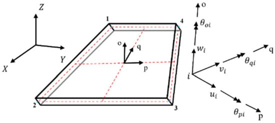
In this section, the four-node element in inverse finite element theory is first introduced. As one of the most efficient inverse finite elements currently available, the four-node quadrilateral element was initially proposed by Kefal [17]. Each node of this element possesses six degrees of freedom (DOFs), including rotations about the coordinate axes, which allows it to better accommodate the deformation of complex structures under load. The specific details of this element are illustrated in Figure 1.

Figure 1. Four-node quadrilateral element, DOF corresponding to local coordinates $(p,q,o)$ and global coordinates $(X,Y,Z)$. At node $i=1,\dots ,4$, $u_i$, $v_i,$ and $w_i$ denote translations along the local $p$, $q$ and $o$ axes, respectively; ${\theta }_{pi}$, ${\theta }_{qi}$ and ${\theta }_{oi}$ denote rotations about these axes. The $p$ and $q$ axes lie in the element midsurface, and $o$ is normal to it. The red dashed lines mark the element midsurface.

First, it is necessary to define a set of convenient coordinate frames of reference so that the geometric properties of the assembled shell structure are unique (as shown in Figure 1). The global coordinate system consists of the $X$-axis, $Y$-axis and $Z$-axis, and the local coordinates consist of the $p$-axis, $q$-axis, and $o$-axis.

The specific shape functions are shown in Appendix A. Through the nodal displacement ${\mathit{u}}^e$, the in-plane and lateral deformation vectors within the element can be obtained by the following equations:

$$\mathit{\epsilon }=\mathit{e}+z\mathit{\kappa }=\left({\mathit{B}}^{\mathrm{m}}+z{\mathit{B}}^{\mathrm{b}}\right){\mathit{u}}^e$$

(1)

$$\mathit{\gamma }={\mathit{B}}^{\mathrm{s}}{\mathit{u}}^e$$

(2)

$${\mathit{u}}^e={\left[{\mathit{u}}_1^e {\mathit{u}}_2^e {\mathit{u}}_3^e {\mathit{u}}_4^e\right]}^{\mathrm{T}}$$

(3)

Here, $\mathit{e}$ is the membrane strain vector, $\mathit{\kappa }$ is the curvature vector, $\mathit{\gamma }$ is the transverse shear strain vector, and $z$ is the thickness coordinate. The element displacement vector contains $u$, $v$, $w$, ${\theta }_x$, ${\theta }_y$ and ${\theta }_z$ at each of its four nodes. The strain–displacement matrices ${\mathit{B}}^{\mathrm{m}}$, ${\mathit{B}}^{\mathrm{b}}$ and ${\mathit{B}}^{\mathrm{s}}$ are defined in Appendix B.

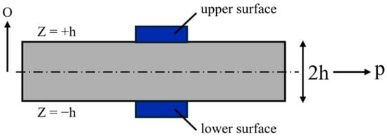
At an instrumented element, three in-plane strain components on each face, ${\mathit{\xi }}^{+}$ and ${\mathit{\xi }}^{-}$, determine the membrane strains and curvatures through Equation (4). The plate thickness is $2h$. A sensor site in the numerical optimization denotes this upper/lower measurement pair; sensor counts in Section 3 refer to sites, so that 23 sites correspond to $23\times 2$ surface rosettes. Figure 2 shows the corresponding surface sensor arrangement.

$$\left[{\mathit{e}}^{\mathrm{m}} {\mathit{\kappa }}^{\mathrm{m}}\right]=\left[{\displaystyle \frac{1}{2}}\left({\mathit{\xi }}^{+}+{\mathit{\xi }}^{-}\right) {\displaystyle \frac{1}{2h}}\left({\mathit{\xi }}^{+}-{\mathit{\xi }}^{-}\right)\right]$$

(4)

Figure 2. Specific arrangement of sensors. The local $p$ and $o$ axes indicate the in-plane and thickness directions, respectively. Here, $h$ is the half-thickness and $2h$ is the total thickness. The labels $Z=+h$ and $Z=-h$ mark the upper and lower surfaces, respectively; $Z$ in this schematic is the local through-thickness coordinate measured from the midsurface, denoted $z$ in Equation (1).

For each element with area $A_e$, the least squares functional is written as follows:

$${\Phi }^e={\int }_{{\mathrm{A}}_e}\left[{\omega }_e{‖\mathit{e}-{\mathit{e}}^{\mathrm{m}}‖}^2+{\omega }_{\kappa }{\left(2h\right)}^2{‖\mathit{\kappa }-{\mathit{\kappa }}^{\mathrm{m}}‖}^2+{\omega }_{\gamma }{‖\mathit{\gamma }‖}^2\right]\mathrm{d}A$$

(5)

The membrane and bending weights are ${\omega }_e={\omega }_{\kappa }=1$ at instrumented elements and ${10}^{-4}$ at uninstrumented elements. For an uninstrumented element, the observation vector is set to zero: the small weights provide regularization without introducing strain values from unsensed locations into the right-hand side. In Section 3, unmeasured transverse shear is regularized with ${\omega }_{\gamma }={10}^{-5}$ and zero shear observations. The factor ${\left(2h\right)}^2$ gives the curvature term the same dimensions as the membrane term. Element matrices are integrated with $2\times 2$ Gauss quadrature and assembled after applying the prescribed displacement boundary conditions.

By minimizing the functional $\Phi$, the stiffness matrix of the element in the local coordinate system can be obtained:

$${\displaystyle \frac{\mathsf{\partial }\varphi }{\mathsf{\partial }{\mathit{u}}^e}}={\mathit{k}}^e{\mathit{u}}^e-{\mathit{f}}^e=0\Rightarrow {\mathit{k}}^e{\mathit{u}}^e={\mathit{f}}^e$$

(6)

Here, ${\mathit{k}}^e$, ${\mathit{f}}^e,$ and ${\mathit{u}}^e$ are the element matrix, observation-dependent right-hand side, and nodal displacement vector. Assembly gives the global linear system. Translational and rotational magnitudes can be calculated from Equations (7) and (8), respectively.

$$U_T=\sqrt{U^2+V^2+W^2}$$

(7)

$${\theta }_T=\sqrt{{\left({\theta }_X\right)}^2+{\left({\theta }_Y\right)}^2+{\left({\theta }_z\right)}^2}$$

(8)

2.2. NSGA-III with Lichtenberg-Inspired Local Search

NSGA-III selects nondominated solutions using reference directions [16], whereas NSGA-II uses crowding distance [18]. The directions follow the Das–Dennis construction [19]. The general formulation contains one residual per training load and a sensor-count objective. The controlled comparisons fix the count at 23 sites and omit this constant objective, giving two objectives for A/B and three for C/D/E. NSGA-II provides an additional control for the A/B comparison.

The additional operator explores the neighborhood of first-front solutions through stochastic discharge moves. The Lichtenberg algorithm draws inspiration from branched discharge patterns [15,20], whose physical background includes diffusion-limited aggregation (DLA) [21,22]. Multi-objective Lichtenberg optimization extends this concept to engineering problems [23]. The present operator generates directions or binary masks directly. It does not simulate a DLA particle cluster and therefore has no particle count, adhesion or creation radius parameters.

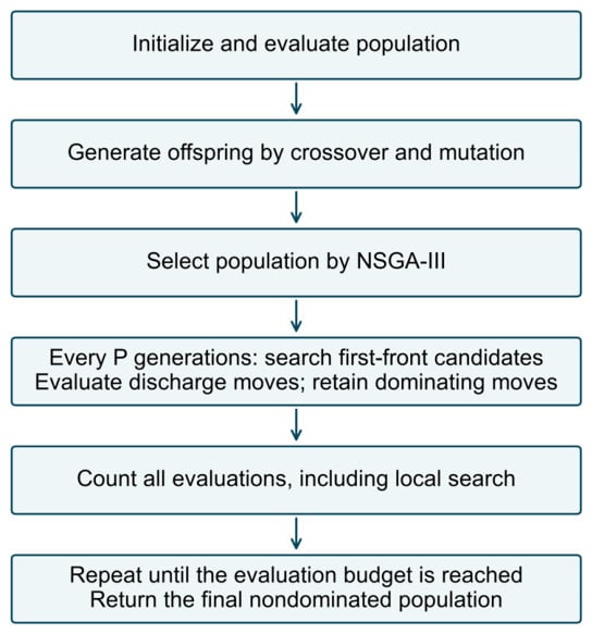
Figure 3 summarizes the algorithm. Local search is invoked after every $P=5$ completed offspring generations. Each candidate receives up to two trials for continuous benchmarks or six for binary placement, with energy reset and decayed according to Equation (9). Only if a trial Pareto-dominates its parent does it replace the parent. The next environmental selection step reassociates the updated population with the reference directions.

$$E_j=\max \left(E_{\min },E_0{a}^j\right),\hspace{1em}j=1,\dots ,M_{\mathrm{ls}}$$

(9)

Figure 3. LA-NSGA-III procedure. The objective-evaluation counter includes initialization, evolutionary offspring and every local search trial.

Table 1 and Table 2 specify the local search procedure and its continuous and binary moves. Both representations use the same energy law and dominance acceptance rule. The binary move exchanges active and inactive sites, preserving the prescribed sensor count. Section 2.4 gives one fixed configuration for the continuous benchmarks and one for numerical placement; development runs and reported confirmation runs are separated (Section 2.4).

Table 1. Lichtenberg-inspired local search procedure.

Step	Operation
1	Select the first nondominated front of the current population. If necessary, sample at most $N_{\mathrm{c}}$ candidates without replacement.
2	Initialize an empty tabu list for this invocation. For each candidate $\mathit{x},$ set the current objective vector to $\mathit{F}(\mathit{x}).$
3	For $j=1,\dots ,M_{\mathrm{ls}},$ stop if the evaluation budget has been consumed; otherwise, compute $E_j$ using Equation (9).
4	Generate one trial using Table 2, repair bounds or sensor count constraints, and evaluate its complete objective vector. Increment NFE by one.
5	If the trial is no worse in every objective and better in at least one, replace $\mathit{x}$ and store the accepted direction in the tabu list.
6	Return the updated population. All trials count toward the budget, including rejected or repeated candidates.

NFE: number of objective-function evaluations; $N_{\mathrm{c}}$: candidate limit (24 for three-objective DTLZ, 53 for five-objective DTLZ, and 60 for placement); $M_{\mathrm{ls}}$: maximum trials per candidate; $\mathit{F}$: objective vector. A single evaluation computes all objectives of one candidate.

Table 2. Discharge move generation in the two decision spaces.

Representation	Operation
Continuous	Draw and normalize a standard-normal base direction. Use $b=\max \left(1,\min \left(\mathrm{Poisson}\left(2E\right),3\right)\right)$ branches. For each branch, rotate two randomly selected coordinates through $\mathsf{\pi }(0.1+0.8U)$ and add the direction with weight $E(0.5+U).$ Normalize the sum to length $E.$
Continuous repair	If cosine similarity to an accepted direction exceeds 0.9, multiply its coordinates by independent factors $0.5+U$ before normalization. Coordinates below/above $[0,1]$ are reset within the lower/upper 10% of the interval.
Binary	Draw a Poisson variate with mean twice the current energy, add one and cap the branch count at three. Multiply this count by $\max \left(1,\mathrm{round}\left(0.3E{n}_{\mathrm{var}}\right)\right)$ and cap the product by the numbers of active and inactive sites. Select this many indices from each set uniformly without replacement, and toggle both subsets.
Binary repeat handling	If the exchange mask repeats an accepted mask, redraw both subsets once. Apply the mask by exclusive OR. The move preserves the parent sensor count; crossover and mutation offspring are separately repaired to the prescribed count.

$E$: current discharge energy; $U$: an independent uniform variate on $[0,1)$; $n_{\mathrm{var}}$: decision vector length; Poisson: Poisson random variate; exclusive OR toggles selected binary bits. The tabu list contains accepted moves from the current invocation only.

DTLZ1, DTLZ2, and DTLZ4 [24] are evaluated with three and five objectives over twenty paired confirmation runs. Table 3 uses identical evaluation caps: 56,494 evaluations for three objectives and 127,412 for five. Paired seeds give the same initial population. Initialization and every local trial count toward the budget, and the final batch is truncated at the exact cap.

Table 3. DTLZ results at exactly equal evaluation budgets.

Task ($\mathit{M}$)	Metric	LA-NSGA-III	NSGA-III	Adjusted $\mathit{p}$
DTLZ1 (3)	HV	$0.84186\pm 0.00011$	$0.84110\pm 0.00092$	<0.0001
DTLZ1 (3)	IGD	$0.04084\pm 0.00007$	$0.04098\pm 0.00021$	$0.0029$
DTLZ1 (5)	HV	$0.97969\pm 0.00009$	$0.97957\pm 0.00016$	$0.0365$
DTLZ1 (5)	IGD	$0.10479\pm 0.00016$	$0.10504\pm 0.00025$	$0.0319$
DTLZ2 (3)	HV	$0.55970\pm 0.00025$	$0.55973\pm 0.00015$	$1.0000$
DTLZ2 (3)	IGD	$0.05400\pm 0.00015$	$0.05406\pm 0.00012$	$0.5309$
DTLZ2 (5)	HV	$0.81170\pm 0.00019$	$0.81190\pm 0.00019$	$0.0365$
DTLZ2 (5)	IGD	$0.16118\pm 0.00008$	$0.16116\pm 0.00008$	$1.0000$
DTLZ4 (3)	HV	$0.55949\pm 0.00091$	$0.54869\pm 0.04961$	$1.0000$
DTLZ4 (3)	IGD	$0.05409\pm 0.00020$	$0.07839\pm 0.10897$	$1.0000$
DTLZ4 (5)	HV	$0.81236\pm 0.00017$	$0.81243\pm 0.00018$	$0.9354$
DTLZ4 (5)	IGD	$0.16108\pm 0.00008$	$0.16108\pm 0.00010$	$1.0000$

Values are mean $\pm$ sample standard deviation over twenty independent confirmation runs. HV: normalized hypervolume (larger is better); IGD: inverted generational distance (smaller is better); DTLZ: Deb–Thiele–Laumanns–Zitzler benchmark; LA: Lichtenberg-inspired local search; NSGA-III: Non-dominated Sorting Genetic Algorithm III. Two-sided paired Wilcoxon tests use Holm correction over the six tasks for each metric. Adjusted $p$-values assess differences; the metric values indicate their direction.

For the performance indicators, DTLZ1 objectives are divided by 0.5, while DTLZ2 and DTLZ4 use scale 1. Hypervolume (HV) [25] is calculated using an $M$-dimensional reference point with all coordinates set to 1.1 and normalized by the reference box volume ${1.1}^M$, where $M$ is the number of objectives. Inverted generational distance (IGD) is the mean distance from an analytical front reference point to its nearest returned solution. The reference sets contain 5050 points for $M=3$ and 4845 for $M=5$, obtained from simplex lattices with 99 and 16 divisions, respectively; for DTLZ2/4, the lattice vectors are normalized to unit Euclidean length. These definitions are fixed across algorithms and runs. HV is compared within each task and dimension, not pooled across dimensions.

With the fixed continuous configuration, LA-NSGA-III improves both HV and IGD on DTLZ1 at both objective dimensions (Holm-adjusted $p$ below 0.05). On DTLZ2 with five objectives, NSGA-III has the higher mean HV by 0.00020 (adjusted $p$ = 0.0365). Thus, the benchmark gains depend on the task. Section 3.3 evaluates the binary local search contribution directly on sensor placement, using identical objectives, variation operators, and evaluation budgets.

2.3. Coupling iFEM with Sensor Layout Optimization

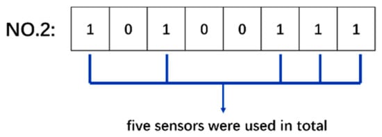
A layout is encoded by a binary vector $\mathit{g}$: $g_e=1$ denotes an instrumented inverse element, and $g_e=0$ denotes an uninstrumented element. Each bit represents an element, and the complete vector is a chromosome. Equation (10) and Figure 4 illustrate the encoding.

$$g_e=\left\{\begin{array}{c}1 \mathrm{e}\mathrm{l}\mathrm{e}\mathrm{m}\mathrm{e}\mathrm{n}\mathrm{t} e \mathrm{w}\mathrm{i}\mathrm{t}\mathrm{h} \mathrm{s}\mathrm{e}\mathrm{n}\mathrm{s}\mathrm{o}\mathrm{r}\mathrm{s} \\ 0 \mathrm{e}\mathrm{l}\mathrm{e}\mathrm{m}\mathrm{e}\mathrm{n}\mathrm{t} e \mathrm{w}\mathrm{i}\mathrm{t}\mathrm{h}\mathrm{o}\mathrm{u}\mathrm{t} \mathrm{s}\mathrm{e}\mathrm{n}\mathrm{s}\mathrm{o}\mathrm{r}\mathrm{s}\end{array}(e=1,2,3\dots ,n_e)\right.$$

(10)

Figure 4. Example chromosome for eight candidate elements. Five elements carry instrumented sites.

Equation (11) gives the general simultaneous minimization formulation: sensor count is scaled by 0.1, and the remaining $L$ objectives are load-specific residuals. The controlled numerical comparisons impose exactly 23 sites throughout each search. On this fixed-count subset, the count objective is constant and is omitted, while the load residuals remain separate objectives. NSGA-III normalizes the objective space during reference direction association; count is not added to the residuals in a scalar fitness.

$$\mathit{f}\left(\mathit{g}\right)={\left[0.1\sum _{e=1}^{n_e}{g}_e,J_1\left(\mathit{g}\right),\dots ,J_L\left(\mathit{g}\right)\right]}^{\mathrm{T}}$$

$$g_e\in \left\{0,1\right\},\hspace{1em}1\le \sum _{e=1}^{n_e}{g}_e\le n_{\max }$$

(11)

For each load $l$, the residual is defined using dimensionless component differences:

$$J_l\left(\mathit{g}\right)=\sum _{i=1}^{n_n}\sum _{c\in C}{\phi }_{l,c}{\left({\displaystyle \frac{d_{i,l,c}\left(\mathit{g}\right)-d_{i,l,c}^{\mathrm{ref}}}{s_c}}\right)}^2$$

(12)

Here, $n_e$ and $n_n$ denote the numbers of inverse elements and nodes, respectively; $n_{\max }=30$ is the general upper site count bound, with exactly 23 sites imposed for the controlled numerical comparisons. The component set is $C=\left\{u,v,w,{\theta }_x,{\theta }_y\right\}$. For the controlled numerical comparisons, the reconstructed component $d_{i,l,c}\left(\mathit{g}\right)$ is compared with the corresponding forward-FE design reference at the inverse mesh node. The reference uses the forward transverse displacement and two bending rotations; the in-plane displacements are zero for these linear pure-bending cases. The dimensional scales are $s_u=s_v=s_w=1\mathrm{mm}$ and $s_{{\theta }_x}=s_{{\theta }_y}=1\mathrm{rad}$. They ensure invariance to the numerical units when converted consistently. The dimensionless weights are ${\phi }_{l,u}={\phi }_{l,v}={\phi }_{l,{\theta }_x}={\phi }_{l,{\theta }_y}=1$, with ${\phi }_{\mathrm{A},w}=3000$ and ${\phi }_{\mathrm{B},w}=2700$; ${\phi }_{l,w}=3000$ for the additional loads. These coefficients prioritize transverse deformation. Their sensitivity is examined in Section 2.4.

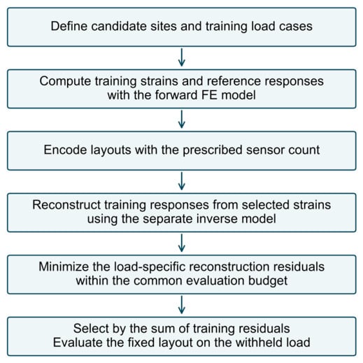
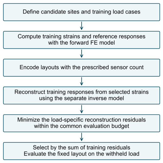
The drilling rotation ${\theta }_z$ remains in the assembled iQS4 system. It is excluded only from the placement objective because the target response here is plate bending, represented by $w$, ${\theta }_x,$ and ${\theta }_y$, and ${\theta }_z$ is an auxiliary in-plane rotational degree of freedom. This does not reduce the element to five degrees of freedom. For the single-objective control, the GA minimizes $J_{\mathrm{A}}$; a second GA control minimizes $J_{\mathrm{A}}+J_{\mathrm{B}}$ with the same fixed sensor count. Figure 5 summarizes how the optimizer evaluates each candidate layout through iFEM.

Figure 5. Coupling of the optimizer with iFEM at a prescribed sensor count. Forward-FE training responses define the design residuals; a separate inverse model reconstructs the responses from the selected strain inputs.

2.4. Parameter Protocol and Sensitivity

Table 4 states the settings used in the computations. Uniform crossover [26] is used for the binary layouts. For the benchmark and controlled numerical comparisons, the standard GA, NSGA-II, and NSGA-III mechanisms use pymoo 0.6.2 [27]; the discharge operator and iQS4 assembly are implemented in Python 3.12. The laboratory layout design and reconstruction routines use MATLAB R2023a (The MathWorks, Inc., Natick, MA, USA). Element operators are derived from the geometry and the shape functions in Appendix A and Appendix B, with derivative and rigid-bending checks. The repeated numerical comparisons use separate random seeds, paired between the compared settings. Computations run on an Intel Core i9-11900K processor (Intel Corporation, Santa Clara, CA, USA) with 64 GB RAM. Reported wall times include model setup, initialization, and optimization; independent runs execute concurrently, so the times describe the batch protocol rather than isolated processor speed.

Table 4. Computational and laboratory layout settings.

Setting	DTLZ Benchmark	Numerical Placement	Laboratory Layout
Decision variables	$M+4$ (DTLZ1); $M+9$ (DTLZ2/4), in $[0,1]$	100 binary elements; exactly 23 selected sites	36 candidate elements; up to 11 sites in design; 10 installed
Population	94 ($M=3$); 212 ($M=5$)	120 for all optimizers	120 in the layout design implementation
Stopping rule	56,494 or 127,412 evaluations, including initialization	36,120 evaluations; final batch truncated at the cap	300 generations for layout design; acquisition uses the fixed mask
Crossover	SBX: probability 1, index 30	Uniform: probability 0.9	Uniform: probability 0.9
Mutation	Polynomial: index 20, probability $1/n_{\mathrm{var}}$ per variable	Bit flip: probability 0.06 per bit	Bit flip: probability 0.06 per bit
Parent selection	Size-2 tournament; random tie-break for feasible NSGA-III individuals	Size-2 tournament; NSGA-II dominance/crowding, GA fitness, NSGA-III feasibility/random	Size-4 tournament with rank/crowding selection
Reference directions	Das–Dennis: 12 divisions/91 directions ($M=3$); 6/210 ($M=5$)	119 divisions/120 directions (A/B, two objectives); 12/91 (C/D/E, three objectives)	3 objectives; 12/91 directions
Local search	$P=5$; $E_0$ = 0.00022344434664; $a$ = 0.25; $E_{\min }$ = 0.000017523285198; $M_{\mathrm{ls}}$ = 2; candidate fraction 0.25 (rounded up)	$P=5$; $E_0$ = 0.1; $a$ = 0.5; $E_{\min }$ = 0.005; $M_{\mathrm{ls}}=6$; $N_{\mathrm{c}}$ = 60	Period 5; 6 trials; initial energy 0.9; decay 0.5; at most 60 first-front candidates
Independent runs	20 confirmation runs per task and algorithm	20 per optimizer for A/B and C/D/E; 5 per setting for formulation and sensitivity	One installed layout; one acquisition record per load case
Seed convention	3,300,000 + 100t + r; t = 0,…,5 for DTLZ1(3), DTLZ1(5), DTLZ2(3), DTLZ2(5), DTLZ4(3), DTLZ4(5)	5,770,000 + r (A/B); 240,000 + r (GA); 5,780,000 + r (C/D/E); 5,890,000 + r (weights)	Session random stream for design; fixed installation indices in Section 4.1

SBX: simulated binary crossover; $M$: objective count; $n_{\mathrm{var}}$: variable count; $r$: run index starting at 1. DTLZ sensitivity uses seeds 3,400,000 + r. Continuous energy constants are rounded here. Every numerical optimizer uses the same repair rule: randomly remove excess sites or add inactive sites until exactly 23 are selected. The laboratory mask is specified directly in Section 4.1. The laboratory column describes pre-installation design; acquisition and reconstruction use the fixed installed mask. Binary sensitivity uses the same five paired seeds as the weight checks.

Continuous parameters are selected using separate development seeds: 24 configurations are screened with 2 runs per DTLZ task, and the 3 leading candidates, the initial setting, and the baseline are evaluated with 4 further runs per task. Selection uses an equal-weight mean paired log-ratio score for HV and IGD across the six tasks. The binary energy constants in Table 4 are retained during development of the count-preserving exchange move, checked with five runs per training-load group. The final operator, parameters, common FE reference and fixed-count comparison protocol are then held fixed for twenty new paired numerical runs. Case F, noise, and site loss results are excluded from training objective and representative layout selection.

Across the six DTLZ tasks, mean elapsed times range from 5.4 to 18.1 s for LA-NSGA-III and from 4.5 to 15.4 s for NSGA-III. LA-NSGA-III completes 545–546 evolutionary generations on average, compared with 600 for NSGA-III. Its local trials use approximately 9.1% of the common evaluation budget. Plate study costs are reported in Section 3.3. Timings describe concurrent batches; the exact evaluation count controls the computational budget.

Table 5 varies $E_0$, $a$, $E_{\min }$ and $P$ around the selected configuration on three-objective DTLZ2, using five paired seeds and 56,494 evaluations. The energy constants are halved or doubled; $a$ takes values of 0.125, 0.25 and 0.5. For $P=1$, $P=5$ and $P=10$, local trials consume 33.7%, 9.2% and 4.8% of the budget, respectively. The selected $P=5$ combines regular refinement with predominantly evolutionary search.

Table 5. Sensitivity of the local search parameters on DTLZ2 with three objectives.

Setting	HV	IGD	Generations
Selected	$0.55958\pm 0.00017$	$0.05411\pm 0.00012$	$545.0\pm 0.0$
$P=1$	$0.55953\pm 0.00028$	$0.05406\pm 0.00018$	$398.0\pm 0.0$
$P=10$	$0.55972\pm 0.00007$	$0.05398\pm 0.00006$	$571.0\pm 0.0$
$E_0$ × 0.5	$0.55964\pm 0.00020$	$0.05409\pm 0.00011$	$545.0\pm 0.0$
$E_0$ × 2	$0.55966\pm 0.00013$	$0.05404\pm 0.00010$	$545.0\pm 0.0$
$a$ = 0.125	$0.55964\pm 0.00020$	$0.05409\pm 0.00011$	$545.0\pm 0.0$
$a$ = 0.5	$0.55976\pm 0.00010$	$0.05406\pm 0.00008$	$545.0\pm 0.0$
$E_{\min }$ × 0.5	$0.55975\pm 0.00011$	$0.05392\pm 0.00009$	$545.0\pm 0.0$
$E_{\min }$ × 2	$0.55979\pm 0.00024$	$0.05406\pm 0.00010$	$545.0\pm 0.0$

Mean $\pm$ sample standard deviation over five paired runs at 56,494 evaluations. “Selected” denotes the continuous configuration in Table 4. Each energy factor row changes only the named constant relative to that configuration; other parameters are fixed. HV and IGD follow Table 3.

Table 6 checks the binary A/B placement problem at exactly 23 sites and 36,120 evaluations using five paired seeds per setting. Initial energy, decay and energy floor are each halved or doubled; the invocation period is 1, 5 or 10. The weight checks multiply both transverse-displacement weights by 0.5 or 2, keeping the other component weights at one. Only the named setting changes in each row. Displacement errors, joint training residual, and overlap with the corresponding default layout quantify accuracy and layout variation; the selected configuration is retained for the main comparisons.

Table 6. Sensitivity of binary placement to local search parameters and displacement weights.

Setting	Error A (%)	Error B (%)	Joint Residual	Sites Shared with Default
Default	0.73 ± 0.07	0.71 ± 0.11	44.7 ± 6.8	23.0/23
Period 1	0.69 ± 0.07	0.76 ± 0.10	45.1 ± 8.9	10.8/23
Period 10	0.73 ± 0.07	0.83 ± 0.06	52.1 ± 1.3	11.0/23
Initial energy × 0.5	0.69 ± 0.09	0.76 ± 0.10	44.7 ± 7.0	12.8/23
Initial energy × 2	0.73 ± 0.03	0.81 ± 0.11	50.2 ± 6.3	12.2/23
Decay 0.25	0.70 ± 0.08	0.81 ± 0.07	48.6 ± 6.8	12.4/23
Decay 1	0.80 ± 0.08	0.90 ± 0.05	60.8 ± 7.4	11.6/23
Energy floor × 0.5	0.73 ± 0.08	0.74 ± 0.12	46.6 ± 10.7	16.0/23
Energy floor × 2	0.76 ± 0.09	0.77 ± 0.07	49.6 ± 4.5	12.4/23
Weights × 0.5	0.73 ± 0.07	0.71 ± 0.11	—	23.0/23
Weights × 2	0.73 ± 0.07	0.71 ± 0.11	—	23.0/23

Errors and joint training residuals are mean ± sample standard deviation over five paired runs (seeds 5,890,001–5,890,005). Default uses Table 4 settings and Section 2.3 weights. Joint residual is the sum of the two load objectives; it is omitted for weight changes because their objective scales differ. The weight multiplier applies to both transverse displacement weights. Site overlap is averaged across corresponding paired 23-site layouts. These runs are separate from the twenty-pair optimizer comparison.

Across the local search perturbations, mean A errors range from 0.69% to 0.80% and mean B errors from 0.71% to 0.90%. For periods 1, 5, and 10, mean joint residuals are 45.1, 44.7, and 52.1, while local trials consume 20.1%, 6.3%, and 4.1% of the evaluation budget, respectively. The default period gives mean A/B errors of 0.73%/0.71% while allocating most evaluations to evolutionary search. The weight multipliers leave all five paired layouts unchanged.

3. Numerical Simulation

The numerical study uses a plate under two mirror-symmetric loads to evaluate the effects of the multi-load objective formulation and the local search operator separately. A forward finite element (FE) model supplies the simulated strain inputs and the reference displacement fields used to evaluate reconstruction errors.

3.1. Forward and Inverse Models

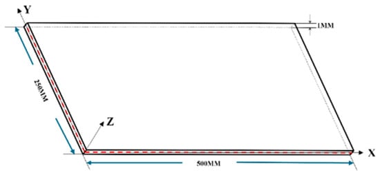
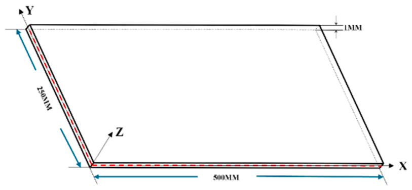
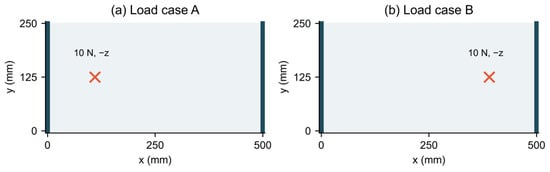
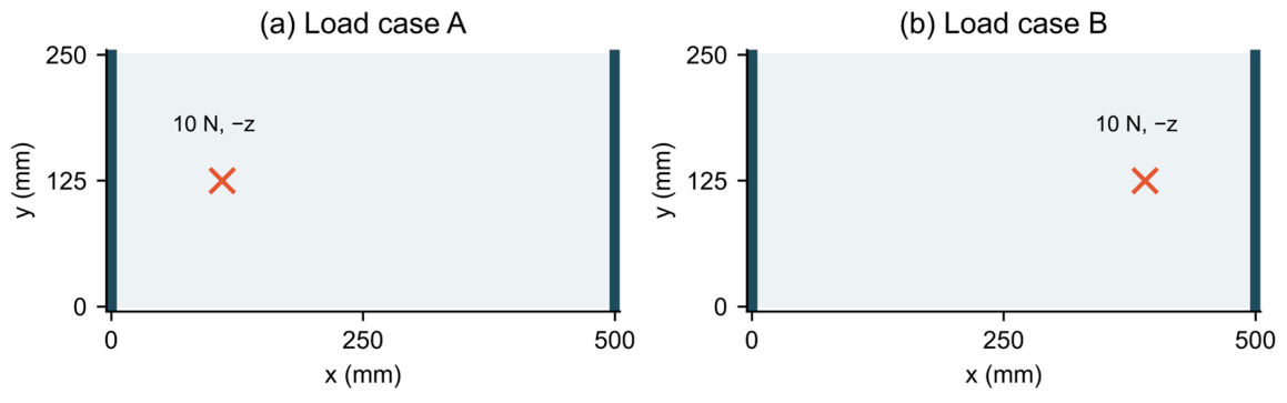
The aluminum plate measures $500\times 250\times 1 \mathrm{mm}$ (Figure 6), with Young’s modulus 71 GPa and Poisson’s ratio 0.33. Both edges $x=0$ and $x=500 \mathrm{mm}$ are fully clamped. Loads A and B are downward 10 N point forces at $(110,125)$ and $(390,125)$ mm, respectively (Figure 7). The two cases are mirror symmetric about $x=250 \mathrm{mm}$. This pair checks transfer between load locations; the distinct load distributions in Section 3.4 provide the additional test of loading-regime coverage.

Figure 6. Dimensions of the numerical plate. Lengths are in mm. The red dashed lines mark the plate midsurface.

Figure 7. Numerical loads and supports. The crosses denote forces acting in the $-z$ direction; thick edges are fully clamped.

The forward solution uses ANSYS Mechanical APDL 2023 R1 (ANSYS, Inc., Canonsburg, PA, USA), linear static analysis, and 5000 SHELL181 elements on a 5 mm square mesh, with 5151 nodes, full integration and stored upper/lower surface strains. The inverse mesh contains $20\times 5=100$ iQS4 elements and 126 nodes. Bilinear interpolation of forward nodal surface strains provides the six input components at each inverse-element center. The different element formulations, mesh densities, and independent assembly avoid identical forward and inverse discretizations. No numerical self-weight is included in Section 3; laboratory self-weight is addressed separately in Section 4.

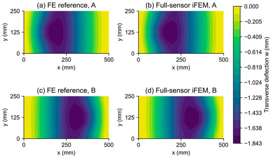
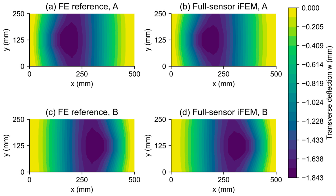
The forward maximum deflection magnitude is 1.8427 mm for each mirror case. With all 100 sites instrumented, the iFEM maximum magnitude is 1.8392 mm, and its relative $L_2$ error is 1.75% for each case (Figure 8). The forward FE fields define both the design residuals and the reported displacement errors. Full instrumentation is a reference configuration rather than an error lower bound: selecting sites changes the weighting of strain fitting on the coarser inverse mesh.

Figure 8. Forward FE reference and full-sensor iFEM reconstruction for loads A and B. All panels use the same color scale; fields are displayed at the inverse mesh nodes. Deflections and coordinates are in mm.

Reconstruction error for a complete load response is evaluated over all inverse mesh nodes by Equation (13). The nodal error uses Equation (14), whose fixed peak response denominator avoids singular relative errors at constrained or zero-displacement nodes.

$$e_l=100{\displaystyle \frac{{‖w_l\left(g\right)-w_l^{\mathrm{FE}}‖}_2}{{‖w_l^{\mathrm{FE}}‖}_2}}$$

(13)

$$e_{i,l}=100{\displaystyle \frac{\left|w_{i,l}\left(\mathit{g}\right)-w_{i,l}^{\mathrm{FE}}\right|}{\underset{k}{\max }\left|w_{k,l}^{\mathrm{FE}}\right|}}$$

(14)

Every numerical optimizer search layout containing exactly 23 sites. The evaluated mask with the lowest sum of training-load residuals is retained; this rule is identical for the multi-objective optimizers and does not use the withheld-load or perturbation results. For the GA controls, the retained mask minimizes the stated scalar objective. The illustrated mask is the run with the median training score, using the lower middle rank for an even number of runs. This common deployment cost isolates differences due to load coverage and the optimizer.

3.2. Effect of Including Both Training Loads

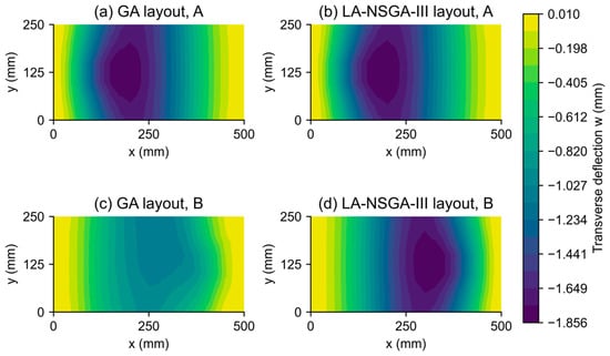
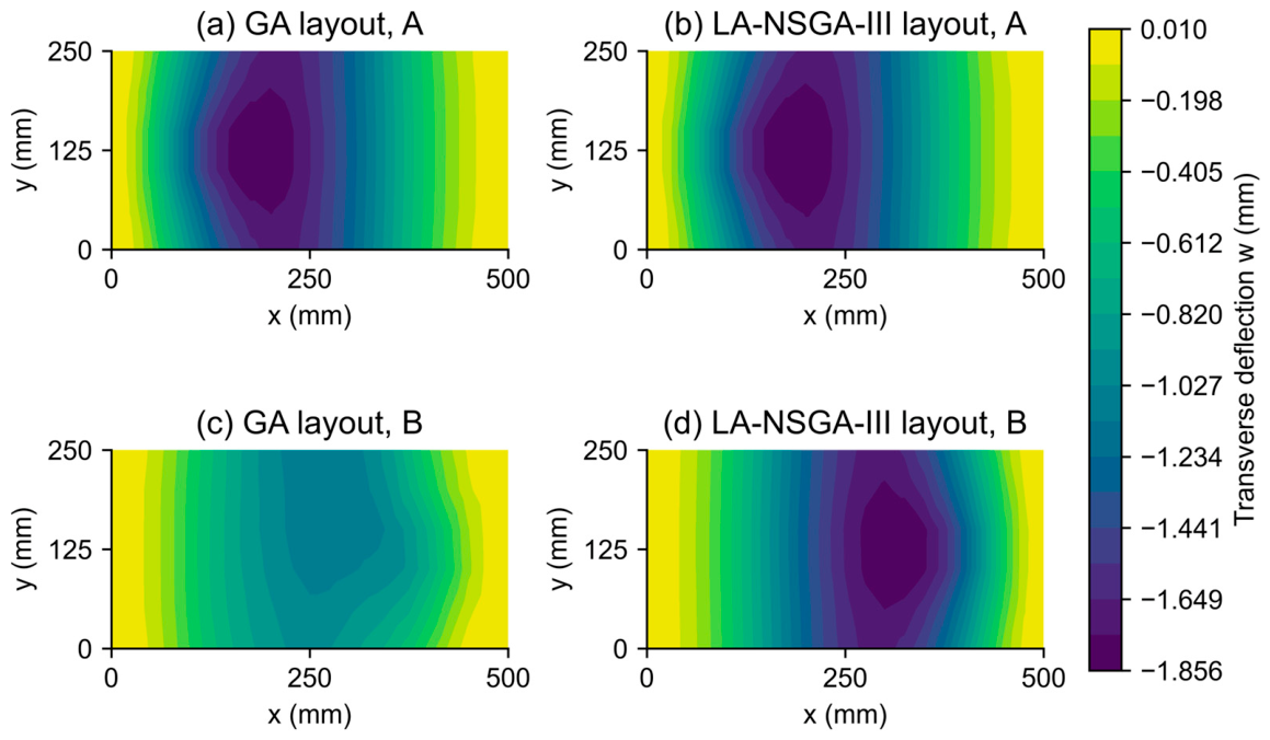
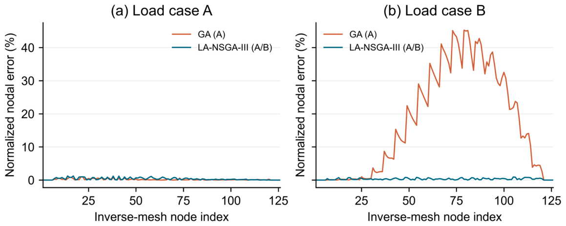
The same GA is run with exactly 23 sites for five paired seeds. The first control minimizes $J_{\mathrm{A}}$, and the second minimizes $J_{\mathrm{A}}+J_{\mathrm{B}}$; crossover, mutation, population and the 36,120-evaluation budget are identical. Mean FE errors are 0.48% on A and 37.70% on B for the single-load control, compared with 0.78% and 0.84% when both loads enter the objective (Table 7). Including B distributes reconstruction accuracy across the two loads rather than concentrating it on A alone.

Table 7. Formulation controls and optimizer comparison at 23 sites and 36,120 evaluations.

Method	Error A (%)	Error B (%)	${\mathit{J}}_{\mathbf{A}}\mathbf{+}{\mathit{J}}_{\mathbf{B}}$	Generations/Time (s)
GA (A)	$0.48\pm 0.03$	$37.70\pm 8.21$	$\mathrm{59,257.7}\pm \mathrm{21,921.3}$	$300.0/89.3$
GA (A + B)	$0.78\pm 0.04$	$0.84\pm 0.07$	$55.8\pm 3.7$	$300.0/89.1$
NSGA-II (A/B)	$0.90\pm 0.13$	$0.89\pm 0.13$	$69.9\pm 11.6$	$300.0/88.5$
NSGA-III (A/B)	$0.84\pm 0.10$	$0.81\pm 0.09$	$59.0\pm 8.5$	$300.0/89.9$
LA-NSGA-III (A/B)	$0.73\pm 0.08$	$0.77\pm 0.10$	$48.0\pm 7.3$	$280.4/91.0$

$J_{\mathrm{A}}$ and $J_{\mathrm{B}}$ are the dimensionless weighted reconstruction residuals defined by Equation (12) for training loads A and B, respectively; $J_{\mathrm{A}}+J_{\mathrm{B}}$ is their joint training residual. Errors and objectives are mean $\pm$ sample standard deviation; generations and elapsed seconds are means. All algorithms search exactly 23-site layouts. The first two rows compare scalar formulations over five paired runs. The final three rows compare multi-objective optimizers over twenty paired runs. Timings follow the concurrent-batch conditions in Section 2.4; all local search evaluations count toward the common cap.

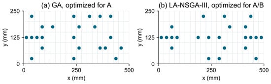
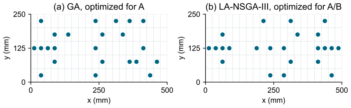
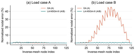
Figure 9 compares representative single-load GA and multi-load LA-NSGA-III layouts, and Figure 10 shows the corresponding reconstructions on common scales. These panels illustrate the complete design strategies. The same-formulation optimizer comparison in Section 3.3 is used to assess the additional local search operator. Figure 11 gives their nodal reconstruction errors.

Figure 9. Representative 23-site layouts, selected by median training score: (a) GA with load A only; (b) LA-NSGA-III with loads A and B. Each marker denotes a paired upper/lower strain measurement site.

Figure 10. Reconstructed transverse deflection fields for the layouts in Figure 9. Panels (a,b) show load A and (c,d) show load B; the two algorithms share a common color scale. The associated quantitative nodal errors are given in Figure 11.

Figure 11. Nodal reconstruction error relative to the forward FE field, normalized by the FE peak-deflection magnitude of each load (Equation (14)). The horizontal coordinate is the inverse mesh node index; the ordinate is a percentage.

3.3. Optimizer Comparison and Computational Cost

LA-NSGA-III, NSGA-III, and NSGA-II are compared on the same two-objective A/B problem at exactly 23 sites, with identical encoding, variation operators, initial populations and evaluation caps. Twenty paired confirmation seeds are used. The GA rows in Table 7 provide the separate scalar formulation controls. Duplicate masks are cached identically for all optimizers; every requested objective evaluation, including a cache hit, counts toward the cap.

LA-NSGA-III reduces the mean joint training residual by 18.65% relative to NSGA-III and 31.36% relative to NSGA-II. Its residual is lower in 17 of 20 NSGA-III pairs and all 20 NSGA-II pairs. Two-sided paired Wilcoxon tests, with Holm adjustment over these two comparisons, give $p$ = 0.0003 and $p$ below 0.0001, respectively. The corresponding mean FE errors are 0.73% and 0.77% for A and B, both below the two multi-objective controls. These comparisons isolate the local search contribution from the choice of training loads.

LA-NSGA-III completes 280.4 evolutionary generations on average, with 6.7% of the common budget assigned to local trials; NSGA-III and NSGA-II complete 300 generations. Its mean elapsed time is 91.0 s under the batch protocol. Layout optimization is performed offline. Once a layout is chosen, reconstruction uses a fixed inverse matrix and the current strain vector, without repeating the search for each measurement frame.

3.4. Distinct Loading Regimes and a Withheld Case

The same plate and supports are subjected to three distinct training regimes: C, a uniform downward pressure of $8\times {10}^{-5} \mathrm{N}/{\mathrm{mm}}^2$ over the plate (10 N total); D, a torsional couple with +5 N at (250,0) mm and −5 N at (250,250) mm; and E, a downward 10 N force at (185,175) mm. At the fixed count of 23 sites, the three reconstruction residuals form the objective vector. A total of 20 paired runs compare LA-NSGA-III and NSGA-III under this common formulation, using 36,120 evaluations per run and the same training-residual selection rule.

Case F combines the pressure from C with a downward 10 N force at $(315,75)$ mm. This force location differs from E. Case F is excluded from the optimization objectives, archive ranking and representative run selection, and the selected layout is applied to it without re-optimization. Table 8 reports reconstruction errors for both optimizers and the full-sensor reference across the three training loads and the withheld load.

Table 8. Reconstruction for three training regimes and a withheld combined load.

Layout	C (%)	D (%)	E (%)	F, Withheld (%)
All 100 sites	1.31	4.32	1.38	1.22
NSGA-III, 23 sites	$3.69\pm 0.63$	$2.57\pm 0.45$	$1.89\pm 0.38$	$4.60\pm 1.24$
LA-NSGA-III, 23 sites	$3.38\pm 0.70$	$2.22\pm 0.36$	$1.57\pm 0.27$	$4.81\pm 0.88$

Relative $L_2$ displacement errors against the independently discretized forward FE model. Optimized layout values are mean $\pm$ sample standard deviation over twenty paired runs. The full-sensor row is a deterministic reference. All layout choices use only C/D/E training residuals.

LA-NSGA-III gives lower mean errors on C, D and E, at 3.38%, 2.22%, and 1.57%, compared with 3.69%, 2.57%, and 1.89% for NSGA-III. The mean joint training residual decreases by 23.40% (paired Wilcoxon $p$ = 0.0001). On the withheld F load, the mean errors are 4.81% and 4.60%, respectively, without re-optimization. This verifies application of the trained layouts to the specified combined load; the training load ranking does not extend to this case. The optimizer benefit is established for the training objectives, while F provides a separate assessment of transfer to an untrained load.

3.5. Strain Noise and Loss of Instrumented Sites

Robustness is evaluated for the representative A/B LA-NSGA-III layout, the representative single-load GA layout and a 23-site space-filling reference. The latter is generated deterministically by starting at the candidate closest to the plate center and repeatedly selecting the candidate with the largest distance to its nearest selected site; ties use the smaller element index. This provides an approximately uniform comparison with exactly the same number of instrumented sites.

Independent zero-mean Gaussian noise is added to each measured upper/lower strain component according to Equations (15) and (16), with $\eta =0.01, 0.02 \mathrm{or} 0.05$. The scale ${\sigma }_{c,l}$ is the root mean square value of that component across all candidate sites in the forward strain field for the corresponding load. Thus, the noise scale is fixed independently of the selected layout. The same 100 noise realizations are used for each layout (seed 270,001); only selected strain inputs enter the inverse right-hand side. Table 9 reports the resulting displacement errors.

$${\epsilon }_{e,c,l}^{\mathrm{noise}}={\epsilon }_{e,c,l}+\eta {\sigma }_{c,l}{z}_{e,c,l},\hspace{1em}{z}_{e,c,l}\sim \mathrm{N}\left(0,1\right)$$

(15)

$${\sigma }_{c,l}=\sqrt{{\displaystyle \frac{{\sum }_{e=1}^{n_e}{\epsilon }_{e,c,l}^2}{n_e}}}$$

(16)

Table 9. Dependence of reconstruction error on strain noise level.

Layout	Noise (%)	Error A (%)	Error B (%)
LA-NSGA-III	0	$0.82\pm 0.00$	$0.67\pm 0.00$
LA-NSGA-III	1	$0.86\pm 0.07$	$0.72\pm 0.06$
LA-NSGA-III	2	$0.96\pm 0.17$	$0.84\pm 0.16$
LA-NSGA-III	5	$1.48\pm 0.55$	$1.38\pm 0.50$
Single-load GA	0	$0.46\pm 0.00$	$39.56\pm 0.00$
Single-load GA	1	$0.53\pm 0.07$	$39.58\pm 0.20$
Single-load GA	2	$0.68\pm 0.20$	$39.60\pm 0.40$
Single-load GA	5	$1.26\pm 0.64$	$39.66\pm 1.01$
Space-filling	0	$31.73\pm 0.00$	$37.24\pm 0.00$
Space-filling	1	$31.73\pm 0.11$	$37.24\pm 0.12$
Space-filling	2	$31.73\pm 0.22$	$37.24\pm 0.24$
Space-filling	5	$31.73\pm 0.55$	$37.25\pm 0.59$

Relative $L_2$ errors against the forward FE displacement, in percent. Non-zero-noise rows give mean $\pm$ sample standard deviation over 100 realizations. The zero-noise row is deterministic and has zero spread. All layouts contain 23 instrumented sites.

Sensor loss is simulated by removing all strain components at one or two instrumented sites. The affected elements revert to the uninstrumented regularization rule of Section 2.1; no strain value is supplied there. All 23 single-site removals and all 253 distinct two-site combinations are evaluated, so failed sites are always among those actually installed. This site loss scenario is conservative for a failure confined to one component of a rosette. Table 10 reports mean and worst-case errors over the removal combinations.

Table 10. Reconstruction after loss of instrumented sites.

Layout	Lost Sites	A: Mean/Worst (%)	B: Mean/Worst (%)
LA-NSGA-III	1	$4.98/48.43$	$4.85/45.37$
LA-NSGA-III	2	$9.18/62.79$	$9.09/59.81$
Single-load GA	1	$6.81/66.05$	$42.71/59.94$
Single-load GA	2	$12.80/74.22$	$45.84/65.04$
Space-filling	1	$32.83/42.14$	$39.33/45.89$
Space-filling	2	$34.12/58.92$	$41.44/54.03$

One lost site removes the upper/lower measurement pair. Results exhaust all 23 single-site and 253 two-site losses for each 23-site layout, with no added noise. Mean and worst refer to relative $L_2$ error across the removal combinations, not repeated loading experiments.

At 5% strain noise, the multi-load layout gives mean errors of 1.48% and 1.38% for A and B (Table 9). The single-load GA retains its emphasis on A, whereas the multi-load layout maintains accuracy across both loads. Under site loss, the optimized layout has lower mean errors than the space-filling control, although some worst-case removals give larger errors (Table 10). Accurate nominal reconstruction therefore needs to be distinguished from tolerance of critical-site failure. Noise and site loss are tested separately. Laboratory element-center marking and gauge–axis alignment address installation; systematic position or orientation errors require a separate calibration model.

4. Laboratory Deformation Reconstruction

A cantilever plate test examines displacement reconstruction using the optimized ten-site layout under two laboratory loads. Calibrated experimental strain inputs drive the iFEM reconstruction, while an FE model calibrated against measured peak displacement provides the reference field. The same installed layout is used for both loads.

4.1. Specimen, Loads and Installed Layout

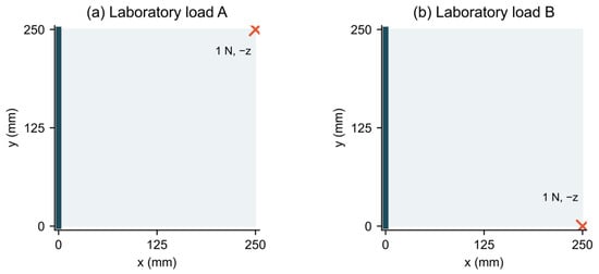
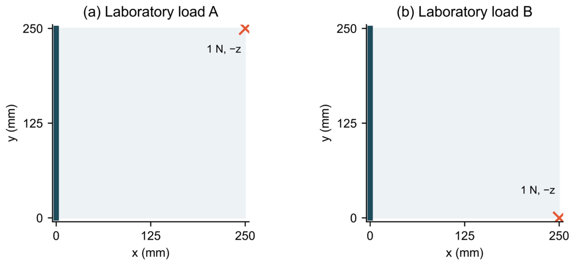
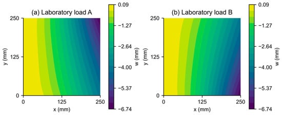
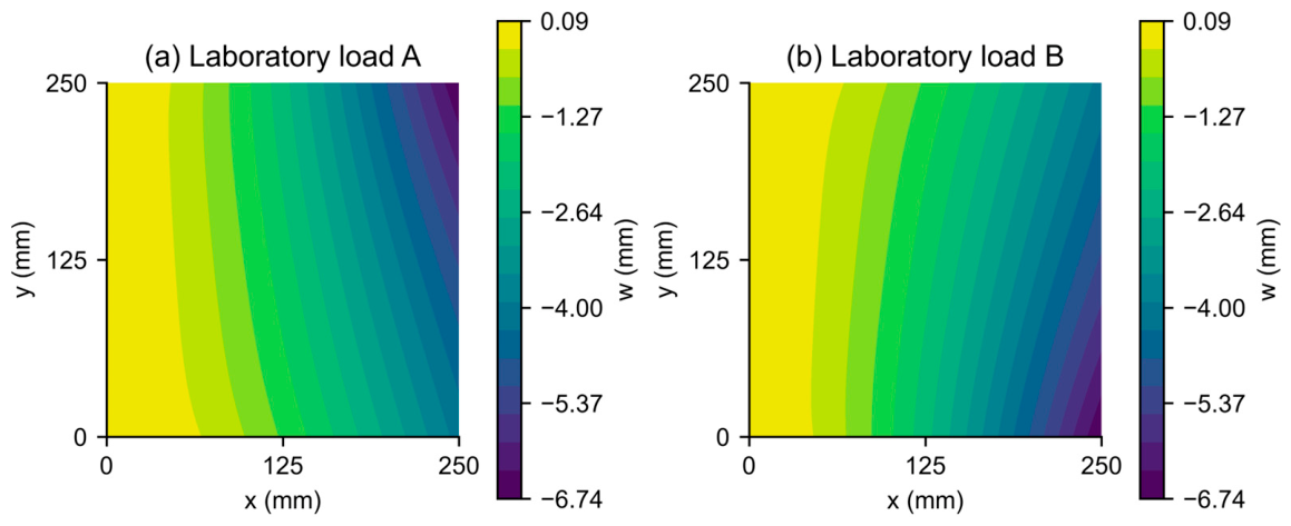
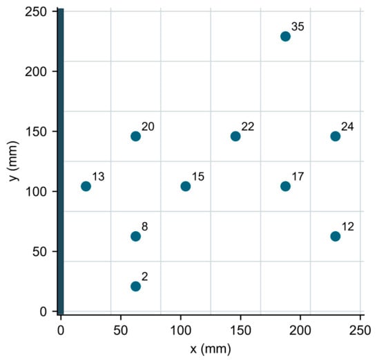
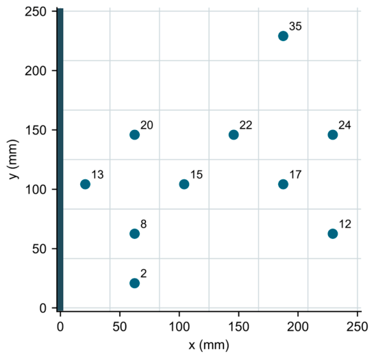
The aluminum specimen is $250\times 250\times 1\mathrm{mm}$, clamped along $x=0$. Two nominal 1 N loads are applied at opposite corners of the free edge (Figure 12). The FE design reference uses a Young’s modulus of 71 GPa, a Poisson’s ratio of 0.33, density of $2770 \mathrm{kg}/{\mathrm{m}}^3$, and gravitational acceleration of $9.80665 \mathrm{m}/{\mathrm{s}}^2$. A 5 mm mesh of 2500 SHELL181 elements gives 2601 nodes. Figure 13 shows these self-weight-included numerical reference fields, with a maximum deflection magnitude of 6.7355 mm for each load. The inverse design grid has $6\times 6=36$ elements and 49 nodes. A total of 10 sites are installed at element indices 2, 8, 12, 13, 15, 17, 20, 22, 24 and 35, with elements numbered along $x$ within each $y$ row (Figure 14). The fixed mask defines the specimen used in the test and is given explicitly for reproduction.

Figure 12. Laboratory plate geometry, clamped edge, and nominal applied forces. The crosses denote forces acting in the negative z direction.

Figure 13. FE reference displacement fields for the laboratory loads, including self-weight. The model is calibrated against laser measurements of peak displacement; the color scales give transverse displacement $w$ in mm.

Figure 14. The 10 installed sites on the 36-element design grid. Labels denote element indices; coordinates are in mm.

Pre-installation layout design uses the two load residuals and the sensor count objective, with at most 11 active sites. Its target responses are full-instrumentation iFEM reconstructions calculated from the corresponding FE strains. Table 4 gives the evolutionary and local search settings. Each local invocation uses six geometrically decreasing energies, from 0.45 to 0.0140625, without an active energy floor. Bit-flip trials are repaired to the upper site count limit. An elite pool contains up to ten members, with an injection probability of 0.2. The physical test uses the specified ten-site layout throughout; Section 3 provides the controlled optimizer comparisons.

4.2. Strain Acquisition and Displacement Reconstruction

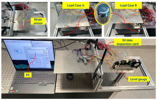
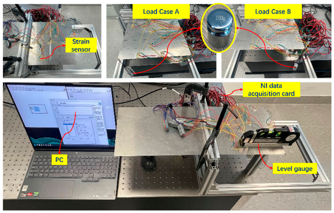
The setup is shown in Figure 15. 120-1AA-S strain gauges with 30 cm preattached leads (CDEM, Chengdu, China) have a nominal resistance of $120 \Omega$ (tolerance $\pm 0.3 \Omega$) and a gauge factor of 2.11 ($\pm 1\%$). Signals are acquired using NI 9235 quarter-bridge modules and an NI cDAQ-9178 chassis with LabVIEW 2021 (National Instruments Corporation, Austin, TX, USA). The plate grid and element centers are marked before bonding. The nominal gauge factor supplies the strain conversion; bridge balancing is performed before loading to remove the initial electrical offset associated with the bonded gauges and lead wires.

Figure 15. Laboratory installation, load application, acquisition equipment, and level gauge (GREENER; Yantai Lvlin Tools Co., Ltd., Yantai, China).

Before bridge balancing, the plate is temporarily supported in a horizontal configuration. The temporary support is then removed, and the external load is applied. The recorded strains describe changes from this supported horizontal reference, including the subsequent response to self-weight and the applied load. Self-weight is therefore retained in the FE reference in Figure 13, and no numerical gravity subtraction is applied to the measured strain records.

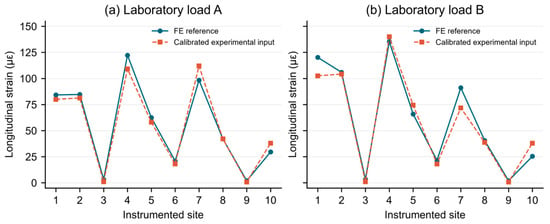
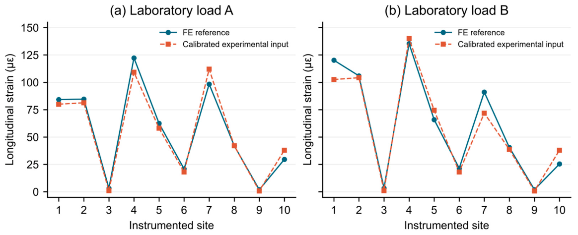
The sampling interval is 0.2 ms (5 kHz). The reported results use one recorded acquisition for each load case on the same specimen. Channel readings are averaged for the static analysis, and the calibrated strain values are assigned to the ten installed element indices in Section 4.1. The same strain inputs supply the iFEM reconstruction and the longitudinal-strain comparison with FE in Figure 16. The laboratory reconstruction uses ${\omega }_{\gamma }={10}^{-10}$ for unmeasured transverse shear; uninstrumented elements provide only matrix regularization, with zero strain observations.

Figure 16. Longitudinal strain at the ten installed sites for loads (a) A and (b) B: calibrated experimental inputs used by iFEM and corresponding FE reference values. Site order follows Section 4.1; strain is in microstrain ($\mathsf{\mu }\mathsf{\epsilon }$).

The peak transverse displacement under each laboratory load is measured manually using an SD-C050 laser displacement sensor (Shenzhen SinceVision Technology Co., Ltd., Shenzhen, China), with displacement expressed in millimeters. The FE model is calibrated against these peak measurements and supplies the reference displacement fields in Figure 13. This peak calibration supports use of the model as a reference; it does not constitute an independent measurement of the complete displacement field.

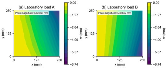
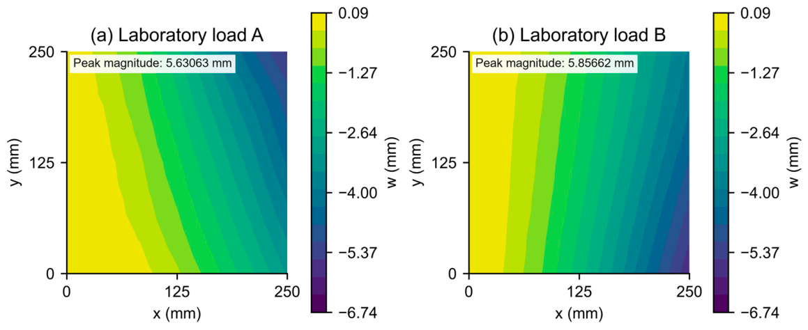
Figure 17 shows the iFEM displacement fields reconstructed from these calibrated experimental strain inputs. The fields capture the cantilever bending pattern and the shift of the maximum-deflection region with load position. Figure 13 and Figure 17 use the same displacement color scale to compare the FE reference with the reconstruction.

Figure 17. Transverse displacement reconstructed by iFEM from the calibrated experimental strain inputs for laboratory loads (a) A and (b) B, using the same color scale as Figure 13. Displacements and coordinates are in mm.

The reconstructed peak displacement magnitudes are 5.63063 and 5.85662 mm for A and B, compared with 6.73550 mm for the FE reference in both cases. Relative peak differences are 16.40% and 13.05%; the relative $L_2$ field differences (Equation (13)) are 17.82% and 9.03%, respectively. The peak difference is normalized by the FE peak magnitude. FE values are assigned to the 49 inverse mesh nodes by nearest-node sampling, and both metrics use the displacement vectors plotted in Figure 17. These are differences from the calibrated FE reference. The test demonstrates strain-based reconstruction with one installed layout under both loads; Section 3.2 and Section 3.3 separately assess the formulation and optimizer effects.

5. Conclusions

A multi-load iFEM placement formulation and LA-NSGA-III search support a common layout for anticipated load responses. With the GA and 23-site count fixed, including both mirror loads reduces the mean second-load error from 37.70% to 0.84%. On the same two-objective placement problem, LA-NSGA-III reduces the mean joint training residual by 18.65% relative to NSGA-III at exactly 36,120 evaluations over 20 paired runs. Its mean FE errors are 0.73% and 0.77% for the two loads. The three-regime C/D/E study also gives lower mean training load errors than NSGA-III, supporting the local search contribution beyond the mirror pair.

The withheld combined load and perturbation tests assess use of the fixed layouts beyond nominal training conditions. They establish the reported transfer and noise performance while identifying sensitivity to critical-site loss. The benchmark and withheld-load results delimit the scope of the optimizer gains. The cantilever test demonstrates displacement reconstruction from calibrated experimental strains using the same installed layout for both loads, with the FE reference calibrated against laser measurements of peak displacement. Together, the numerical and laboratory evidence supports offline design and practical installation of a common sensor layout for iFEM monitoring across a defined set of anticipated loading regimes.

Future work will focus on extending the framework to curved shells and time-varying loads and incorporating sensor failure tolerance and installation uncertainty directly into the placement objectives. Repeated experiments with independent full-field displacement measurements will also be conducted to further evaluate reconstruction accuracy and robustness.

References

- Li, J.; Huang, J.; Bao, X.; Shen, J.; Chen, X.; Cui, H. Tunnel intelligent monitoring and early warning system integrating multi-source data: Methods, architecture, and engineering practices. Tunn. Undergr. Space Technol. 2026, 168, 107142. [Google Scholar] [CrossRef] [Scilit]
- Aroquipa, H.; Hurtado, A.; Angel, C. Methodological framework for integrating structural health monitoring and digital-twin models for seismic assessment of heritage buildings: Case study of Basilica Maria Auxiliadora, Lima, Peru. In Structures; Elsevier: Amsterdam, The Netherlands, 2025; Volume 80. [Google Scholar]
- Aroquipa, H.; Hurtado, A.; Murga, C.; De La Cruz, R.; Tarque, N. Towards Smart Cities: Foundational Methodology for Implementing Intelligent Circular Resilience in Heritage Buildings through Structural Health Monitoring and Digital-Twins–Part A. Int. J. Disaster Risk Reduct. 2025, 128, 105749. [Google Scholar] [CrossRef] [Scilit]
- Tessler, A.; Spangler, J.L. A Variational Principle for Reconstruction of Elastic Deformations in Shear Deformable Plates and Shells; National Aeronautics and Space Administration, Langley Research Center: Hampton, VA, USA, 2003.
- Zhao, F.; Du, R.; Wang, J.; Zhang, F.; Hong, B. Geometrically nonlinear shape sensing of anisotropic composite beam structure using iFEM algorithm and third-order shear deformation theory. Compos. Struct. 2023, 322, 117364. [Google Scholar] [CrossRef] [Scilit]
- Roy, R.; Tessler, A.; Surace, C.; Gherlone, M. Efficient shape sensing of plate structures using the inverse Finite Element Method aided by strain pre-extrapolation. Thin-Walled Struct. 2022, 180, 109798. [Google Scholar] [CrossRef] [Scilit]
- Craiu, I.D.; Nedelcu, M. Combining iFEM and GBT for accurate shape sensing and damage detection in truncated conical shells with circular cross-section. Ocean Eng. 2024, 311, 118811. [Google Scholar] [CrossRef] [Scilit]
- Khalid, I.; Qureshi, Z.A.; Oterkus, S.; Oterkus, E. Structural Health Monitoring of aerospace thin plate and shell structures using the inverse finite element method (iFEM). Thin-Walled Struct. 2025, 209, 112923. [Google Scholar] [CrossRef] [Scilit]
- Li, M.; Kefal, A.; Oterkus, E.; Oterkus, S. Structural health monitoring of an offshore wind turbine tower using iFEM methodology. Ocean Eng. 2020, 204, 107291. [Google Scholar] [CrossRef] [Scilit]
- Zhan, J.Z.; Hong, K.; Liu, G. An improved inverse finite element method based on co-rotational coordinates for reconstructing geometrically nonlinear shell deformations. Thin-Walled Struct. 2025, 215, 113569. [Google Scholar] [CrossRef] [Scilit]
- Ghasemzadeh, M.; Kefal, A. Sensor placement optimization for shape sensing of plates and shells using genetic algorithm and inverse finite element method. Sensors 2022, 22, 9252. [Google Scholar] [CrossRef] [Scilit] [PubMed]
- Reeves, C.R. Genetic algorithms. In Handbook of Metaheuristics; Springer: Boston, MA, USA, 2010; pp. 109–139. [Google Scholar]
- Li, X.; Niu, S.; Bao, H.; Hu, N. Improved adaptive multi-objective particle swarm optimization of sensor layout for shape sensing with inverse finite element method. Sensors 2022, 22, 5203. [Google Scholar] [CrossRef] [Scilit] [PubMed]
- Roy, R.; Tessler, A.; Surace, C.; Gherlone, M. Shape sensing of plate structures using the inverse finite element method: Investigation of efficient strain–sensor patterns. Sensors 2020, 20, 7049. [Google Scholar] [CrossRef] [Scilit] [PubMed]
- Pereira, J.L.J.; Francisco, M.B.; Diniz, C.A.; Oliver, G.A.; Cunha, S.S., Jr.; Gomes, G.F. Lichtenberg algorithm: A novel hybrid physics-based meta-heuristic for global optimization. Expert Syst. With Appl. 2021, 170, 114522. [Google Scholar] [CrossRef] [Scilit]
- Deb, K.; Jain, H. An evolutionary many-objective optimization algorithm using reference-point-based nondominated sorting approach, part I: Solving problems with box constraints. IEEE Trans. Evol. Comput. 2013, 18, 577–601. [Google Scholar] [CrossRef] [Scilit]
- Kefal, A.; Oterkus, E.; Tessler, A.; Spangler, J.L. A quadrilateral inverse-shell element with drilling degrees of freedom for shape sensing and structural health monitoring. Eng. Sci. Technol. An. Int. J. 2016, 19, 1299–1313. [Google Scholar] [CrossRef] [Scilit]
- Deb, K.; Pratap, A.; Agarwal, S.; Meyarivan, T. A fast and elitist multiobjective genetic algorithm: NSGA-II. IEEE Trans. Evol. Comput. 2002, 6, 182–197. [Google Scholar] [CrossRef] [Scilit]
- Das, I.; Dennis, J.E. Normal-boundary intersection: A new method for generating the Pareto surface in nonlinear multicriteria optimization problems. SIAM J. Optim. 1998, 8, 631–657. [Google Scholar] [CrossRef] [Scilit]
- Merrill, F.H.; Von Hippel, A. The atomphysical interpretation of Lichtenberg figures and their application to the study of gas discharge phenomena. J. Appl. Phys. 1939, 10, 873–887. [Google Scholar] [CrossRef] [Scilit]
- Witten, T.A., Jr.; Sander, L.M. Diffusion-limited aggregation, a kinetic critical phenomenon. Phys. Rev. Lett. 1981, 47, 1400. [Google Scholar] [CrossRef] [Scilit]
- Witten, T.A.; Sander, L.M. Diffusion-limited aggregation. Phys. Rev. B 1983, 27, 5686. [Google Scholar] [CrossRef] [Scilit]
- Pereira, J.L.J.; Oliver, G.A.; Francisco, M.B.; Cunha, S.S., Jr.; Gomes, G.F. Multi-objective lichtenberg algorithm: A hybrid physics-based meta-heuristic for solving engineering problems. Expert Syst. Appl. 2022, 187, 115939. [Google Scholar] [CrossRef] [Scilit]
- Deb, K.; Thiele, L.; Laumanns, M.; Zitzler, E. Scalable multi-objective optimization test problems. In Proceedings of the 2002 Congress on Evolutionary Computation, Honolulu, HI, USA, 12–17 May 2002; CEC’02 (Cat. No. 02TH8600); IEEE: Piscataway, NJ, USA, 2002; Volume 1. [Google Scholar]
- Zitzler, E.; Thiele, L. Multiobjective evolutionary algorithms: A comparative case study and the strength Pareto approach. IEEE Trans. Evol. Comput. 1999, 3, 257–271. [Google Scholar] [CrossRef] [Scilit]
- Syswerda, G. Uniform crossover in genetic algorithms. ICGA 1989, 3, 2–9. [Google Scholar]
- Blank, J.; Deb, K. Pymoo: Multi-Objective Optimization in Python. IEEE Access 2020, 8, 89497–89509. [Google Scholar] [CrossRef] [Scilit]
Disclaimer/Publisher’s Note: The statements, opinions and data contained in all publications are solely those of the individual author(s) and contributor(s) and not of MDPI and/or the editor(s). MDPI and/or the editor(s) disclaim responsibility for any injury to people or property resulting from any ideas, methods, instructions or products referred to in the content. |
© 2026 by the authors. Licensee MDPI, Basel, Switzerland. This article is an open access article distributed under the terms and conditions of the Creative Commons Attribution (CC BY) license.