Interface Decomposition and Stagewise Attenuation of Multilayer Ultrasonic Propagation in a Dual-String Wellbore

Abstract

In dual-string wells with retained tubing, ultrasound must pass successively through the wellbore fluid, tubing, annular fluid, casing, cement sheath, and formation. Repeated fluid–solid transitions make signals from the outer layers difficult to separate directly from the final received waveform. This study combined 300 kHz ultrasonic through-transmission experiments with COMSOL simulations, progressing from individual media and fluid–solid combinations to an ideal intact dual-string wellbore. The principal wave packets in the experiments corresponded well to those in the respective models. For the water–steel combination, the characteristic peaks differed in time by 0.66 μs, and the local waveform correlation coefficient was 0.986. A two-dimensional axisymmetric model was then used to compare the envelope peaks of consistently identified early composite responses and cumulative outward work over 0–120 μs at successive radial sections. The responses near the tubing and casing did not decrease monotonically. Local amplitudes could increase even as the wave response continuing outward weakened, and the sections adjacent to the two steel strings exhibited distinct stagewise changes. Interface decomposition relates response changes along the complete propagation path to individual material layers, providing a basis for explaining the formation of weak outer-layer signals in dual-string wells.

1. Introduction

Carbon capture, utilization, and storage (CCUS) places stringent demands on long-term well integrity. Corrosion or debonding of the casing, cement sheath, and adjacent interfaces can weaken zonal isolation [1,2,3,4]. Previous studies have examined well integrity in terms of cement durability and well barriers [5,6]. In wells with retained tubing, ultrasound must also cross the inner string before reaching the outer casing and cement sheath. Understanding how multilayer media affect the received response is therefore important for interpreting ultrasonic monitoring signals in dual-string wells.

Acoustic evaluation of single-casing wells is supported by well-established methods. Wang et al. analyzed casing-wave responses under different measurement configurations [7], and Zeroug et al. reviewed the sensitivity of sonic and ultrasonic methods to casing, cement, and formation properties [8]. Waveform amplitude, propagation velocity, dispersion, and interface slip models have also been used to analyze responses under different casing bonding conditions [9,10,11]. Leaky flexural waves and their transit times have been used to identify interface conditions and recover cement elastic properties [12,13]. These studies show that wave propagation near interfaces carries substantial information about the surrounding media.

Retaining tubing creates a dual-string structure comprising multiple fluid and solid layers. Through theory and experiments, Liu et al. showed that the inner and outer strings undergo coupled vibration through the annular fluid [14]. Numerical simulations by Viggen et al. indicated that later wave packets can carry information about outer media in through-tubing ultrasonic measurements. However, interface reflections and mode conversion make these packets difficult to identify directly [15,16,17]. Experiments with two steel strings further showed that propagation distance, string eccentricity, and bonding conditions all affect the received waveform [18,19]. Although outer media can be probed from inside the well, how successive interfaces alter the final waveform warrants further investigation.

Recent through-tubing acoustic studies have progressed from establishing whether outer-layer signals can be received to determining how they can be used to evaluate outer-layer conditions. Correia et al. developed analytical and numerical models of multilayer cylinders to examine guided waves under intact and debonded conditions [20]. Chen et al. analyzed monopole and dipole fields in double-casing wells and found different sensitivities of casing, external Stoneley, and flexural waves to outer-annulus media and source orientation [21,22]. Chen et al. used Lamb waves to detect channels at double-casing interfaces in successive steps [23]. De Souza et al. combined through-tubing experimental data with machine learning to evaluate cement integrity [24], while Zhang et al. investigated velocity imaging in double-casing wells using numerical wavefields and convolutional networks [25]. Semi-analytical finite elements and full-wave modal decomposition have also provided computational and interpretive tools for complex multistring wavefields [26,27]. These studies mainly analyze the final received waveform or a selected mode. Understanding how weak outer-layer signals develop during propagation requires further separation of the response changes within individual material layers and near adjacent interfaces.

The final received signal in a dual-string well contains reflections, transmissions, and superposed waves from multiple interfaces. Comparing only the transmitted signal and the outermost received waveform cannot readily locate the changes along the path. Here, interface decomposition refers to successive radial extraction of signals in an ideal intact wellbore to examine the response as ultrasound crosses each medium. The method provides an additional way to analyze multilayer propagation and weak deep-layer signals; it does not make an ideal-wellbore baseline a prerequisite for defect identification.

This study combined 300 kHz ultrasonic through-transmission experiments with COMSOL transient simulations, progressing from individual media to fluid–solid combinations and then to a complete dual-string wellbore. Transmission experiments on steel plates, rock cores, cement, and fluids were first compared, and a measured excitation was introduced to improve the numerical waveforms. A clean water/steel plate combination was then used to examine propagation across a fluid–solid interface. A two-dimensional axisymmetric model of an ideal concentric dual-string wellbore was subsequently established to extract waveforms and work across sections along the complete radial path. Interface decomposition converts the combined effects that are difficult to distinguish in the final signal into response changes at successive stages. This approach was used to identify the principal propagation characteristics responsible for weakening deep-layer signals in an ideal intact wellbore.

2. Ultrasonic Propagation in Individual Media and Numerical Model Validation

2.1. Experimental System and Material Testing Method

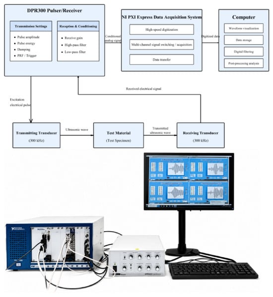
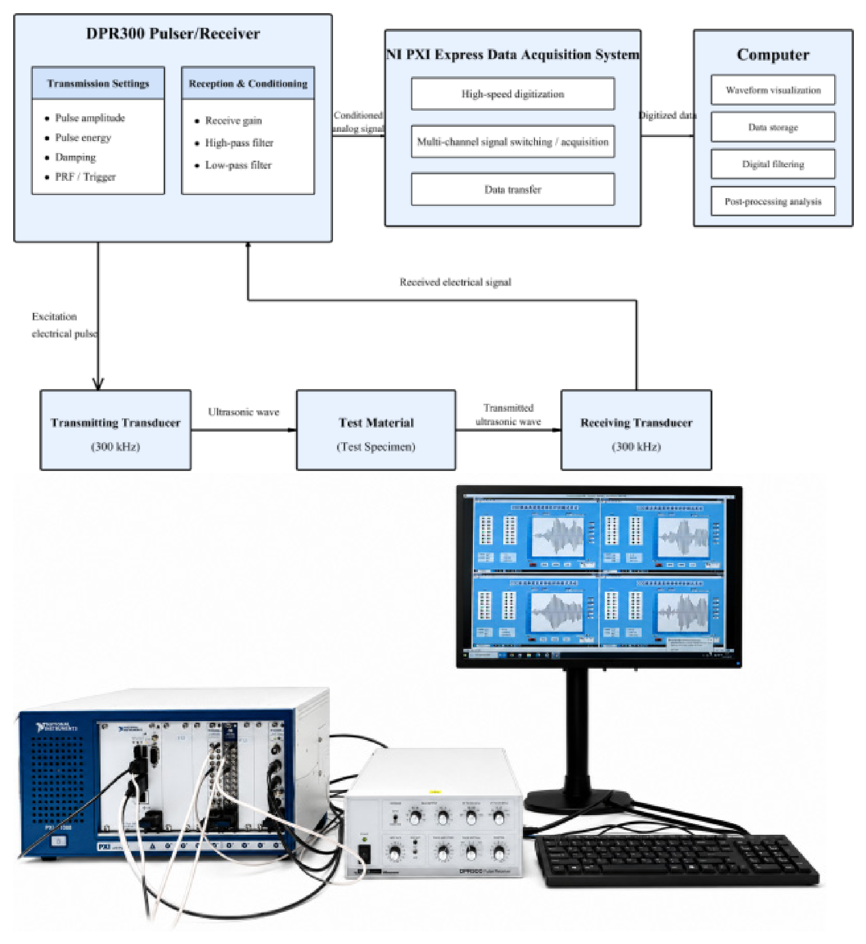
The laboratory ultrasonic system comprised an NI PXI Express acquisition and control platform, a DPR300 pulser–receiver, 300 kHz ultrasonic transducers, and a processing computer. The NI platform used a PXIe-1088 chassis with a PXIe-8821 embedded controller, a PXIe-5122 high-speed digitizer, and a PXIe-2593 multiplexer. It provided 14-bit vertical resolution, a maximum sampling rate of 100 MS/s, and an analog bandwidth of 100 MHz. The multiplexer enabled switching and routing between test channels for recording microsecond-scale signals. The DPR300 generated ultrasonic pulses and provided gain and front-end conditioning for received signals. Its pulse rise time was below 5 ns, and it was compatible with transducers operating from 100 kHz to 50 MHz. The NI platform digitized the conditioned signals, which were displayed, stored, digitally filtered, and analyzed in the time and frequency domains on the computer. The system, processes, and experimental equipment are shown in Figure 1.

Figure 1. Ultrasonic through-transmission system, signal-processing workflow, and laboratory apparatus.

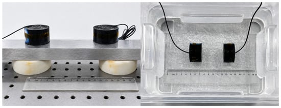
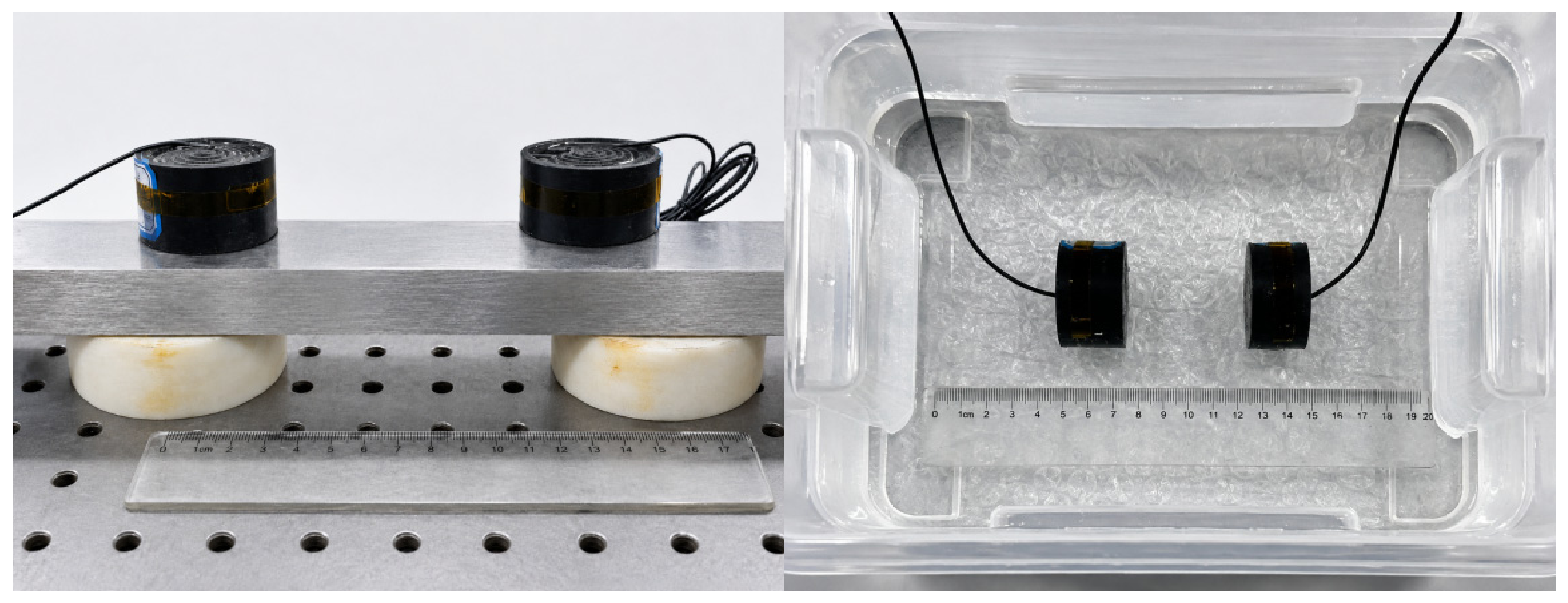
Opposite-side through-transmission experiments were conducted using a transmitting and a receiving transducer with a center frequency of 300 kHz. See Figure 2 for the diagram of ipsilateral and contralateral monitoring. Tests were performed at ambient temperature and pressure on a 20 mm steel plate, a 45 mm water-saturated rock core, and 15 mm water-saturated cement. Clean water and impurity-containing water were also tested, both over a propagation distance of 25 mm. Instrument and receiver settings were kept identical across the tests. Signals sampled at 100 MHz were processed using a Butterworth bandpass filter with a passband of 250–350 kHz. A second-order prototype was transformed into a fourth-order digital bandpass filter and applied using one-way causal filtering. The same processing procedure was used for all datasets.

Figure 2. Same-side transmit–receive and opposite-side through-transmission configurations for ultrasonic testing.

2.2. Experimental Attenuation Characteristics of the Materials

The received reference signal recorded with the two transducers facing each other directly was used as the amplitude baseline. Its maximum absolute amplitude was 216.82 mV. This reference had already passed through the transducers and receiving chain. It therefore reduced, to some extent, the discrepancy between transmitter settings and the actual received response compared with using the pulser output voltage directly. Receiver gain and coupling arrangements were kept consistent for different specimens. Because the measured waveforms could contain later reflections, characteristic peaks were extracted within the actual arrival window of the principal transmitted wave packet. The relative amplitude retention ratio, amplitude attenuation ratio, and insertion loss were then calculated.

Let A_ref be the peak of the direct transducer-to-transducer reference signal and A_m the maximum absolute voltage of the principal wave packet transmitted through a material. The relative amplitude retention ratio R_A, amplitude attenuation ratio η_A, and insertion loss L_A are defined as follows:

R_A = A_m/A_ref

(1)

η_A = (1 − R_A) × 100%

(2)

L_A = 20log₁₀(A_ref/A_m)

(3)

These indices describe the combined transmission response under the specified specimen thickness, material structure, and experimental coupling conditions. They include the effects of propagation within the material and interactions at the specimen surfaces. They can therefore be used to compare the experimental conditions considered here, but do not directly represent intrinsic material absorption coefficients.

2.2.1. Solid Materials

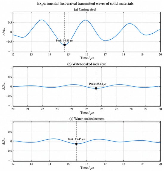
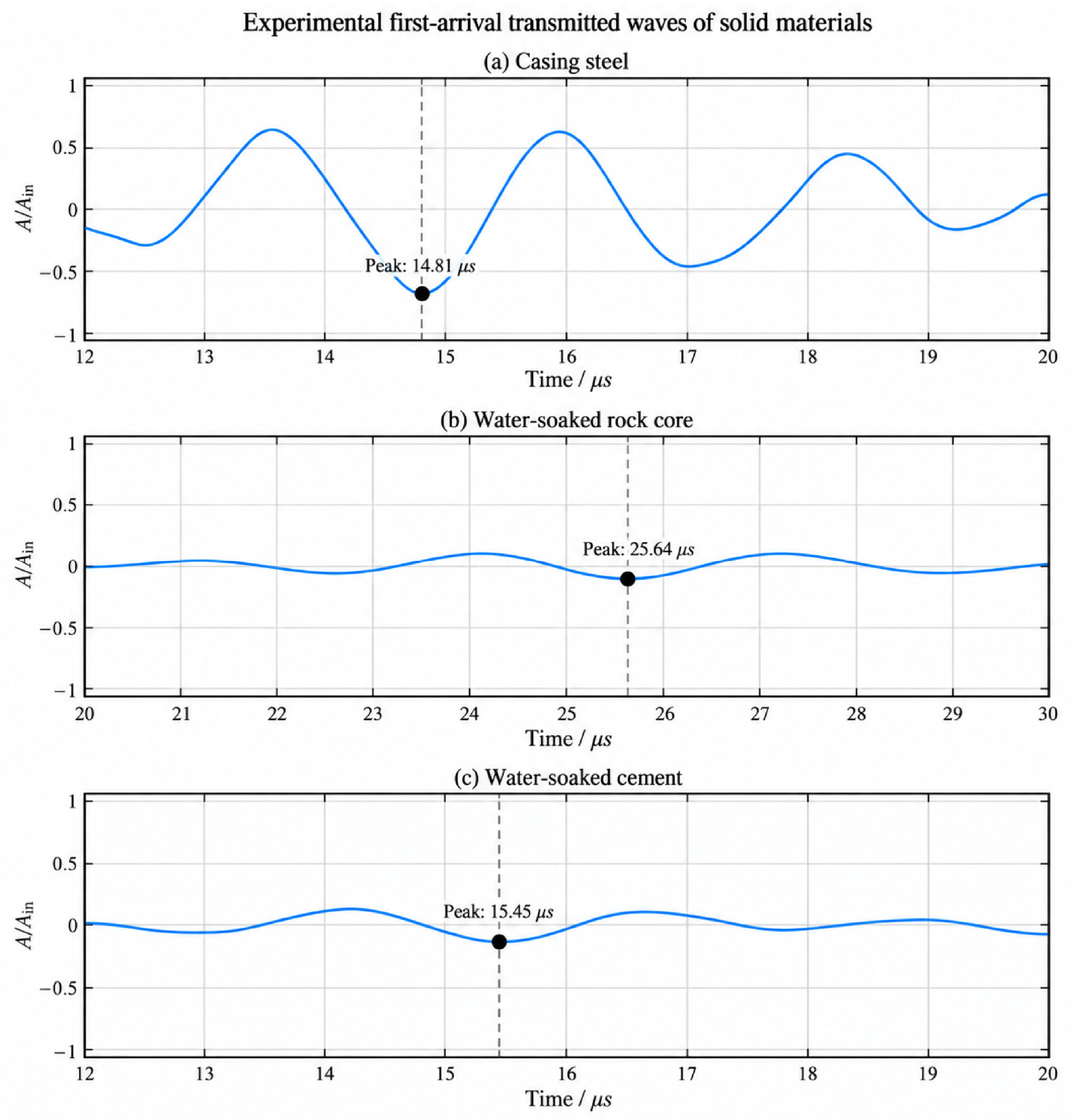
The solid specimens were a 20 mm steel plate, a 45 mm water-saturated rock core, and 15 mm water-saturated cement. Apparent longitudinal velocities calculated from the characteristic peak delays between the reference and principal transmitted wave packets were approximately 6116, 3191, and 3836 m/s, respectively. Evident reports longitudinal velocities of approximately 5850–5890 m/s for selected steels [28], and reported P-wave velocities for water-saturated sandstone are approximately 2950–3300 m/s [29,30]. The measured steel and water-saturated core velocities were close to these ranges, supporting the physical plausibility of the recorded transit delays and first-arrival peak identification.

An analysis window was set for each material according to the position of the principal transmitted wave packet in the received waveform. The maximum absolute amplitude and corresponding peak time were extracted within each window. All solid-material responses were normalized by the direct reference voltage of 216.82 mV for comparison, as shown in Figure 3.

Figure 3. Experimental first-arrival transmitted waves in different solid materials.

Figure 3 shows differences in peak amplitude, principal wave packet shape, and subsequent oscillations among the steel plate, water-saturated cement, and water-saturated core. The peak values and analysis windows are listed in Table 1.

Table 1. Experimental transmission characteristics of first-arrival waves in solid materials.

Material	Thickness/mm	First-Arrival Window/μs	Peak Time/μs	|Am|/mV	RA/%	ηA/%	LA/dB
Casing steel	20	12–20	14.81	147.44	68.00	32.00	3.35
Water-saturated core	45	20–30	25.64	21.85	10.08	89.92	19.93
Water-saturated cement	15	12–20	15.45	28.03	12.93	87.07	17.77

Table 1 shows clear differences in first-arrival transmitted amplitude among the solid media. The steel plate produced a strong transmitted response, whereas the received amplitudes in the water-saturated core and cement were substantially lower. These differences were associated with internal structure, specimen thickness, and interface coupling. The comparatively uniform structure of the steel plate favored preservation of the principal transmitted wave packet. By contrast, pores and heterogeneity in the water-saturated core and cement may have caused scattering and local redistribution of the wavefield, affecting the received response. The amplitude retention ratios were jointly controlled by specimen thickness, water saturation, and interface coupling. They therefore cannot be used to rank the intrinsic attenuation properties of the materials.

2.2.2. Fluid Media

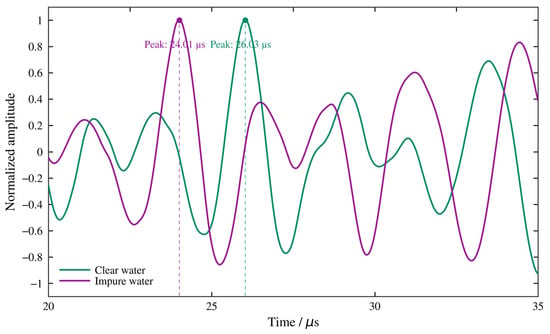
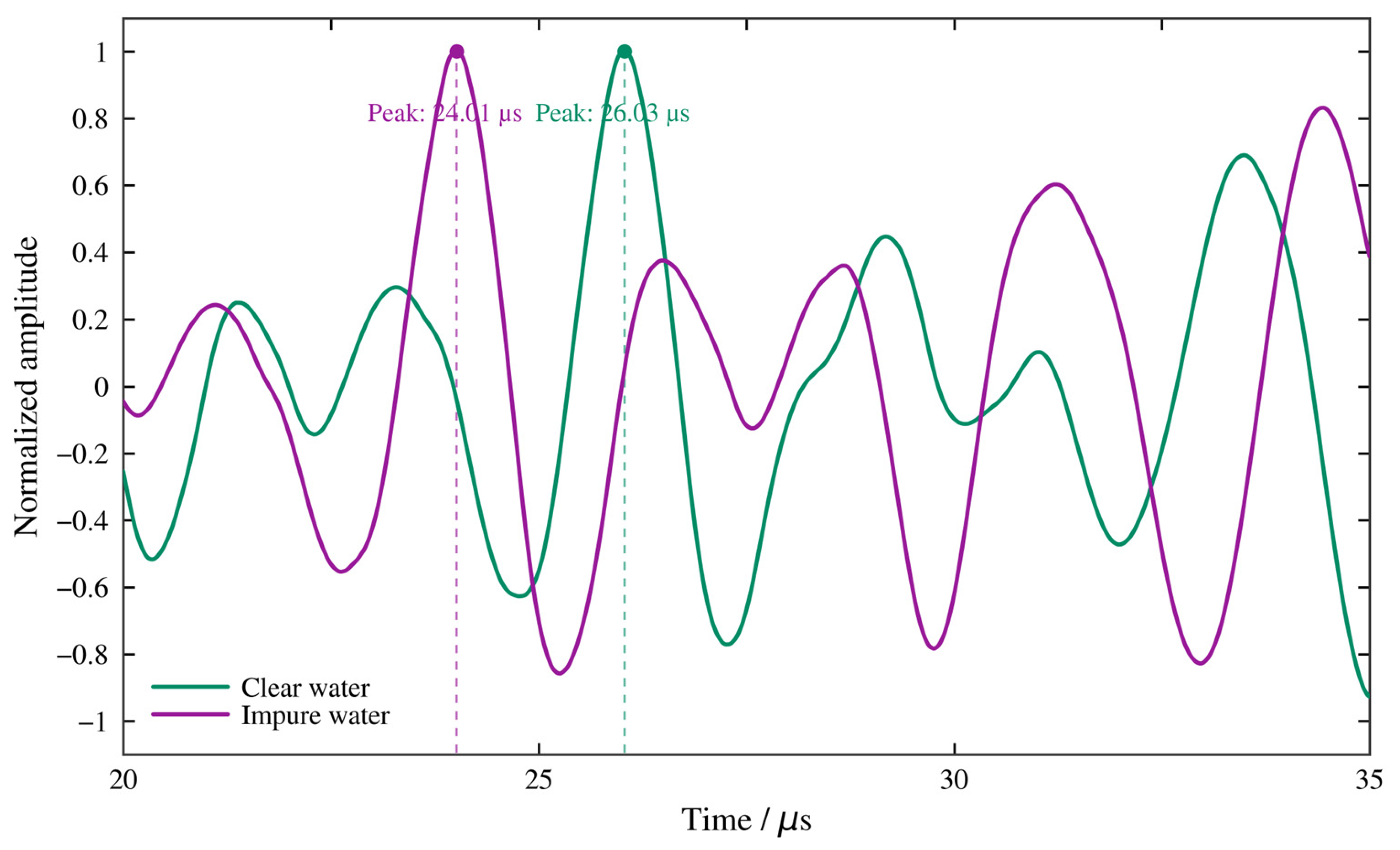
The transmitting and receiving transducers were separated by 25 mm in both clean water and impurity-containing water. The peak time and maximum absolute amplitude of the principal wave packet were extracted within a 20–35 μs window, as listed in Table 2. Because the fluids differed in acoustic properties and later reflections, propagation differences were assessed using waveform shape as well as peak amplitude.

Table 2. Experimental first-arrival results for clean water and impurity-containing water.

Fluid	Path Length/mm	First-Arrival Window/μs	Peak Time/μs	Absolute Peak/mV
Clean water	25	20–35	26.03	229.39
Impurity-containing water	25	20–35	24.01	235.84

To examine how the medium affected the first-arrival wave packet shape, the signals from clean water and impurity-containing water were normalized separately. Their principal oscillatory structures, extrema, and phase changes were compared. The normalized waveforms within the first-arrival window are shown in Figure 4.

Figure 4. Normalized experimental first-arrival waveforms in clean water and impurity-containing water.

At the same propagation distance, the received peak amplitudes differed by approximately 2.8%, indicating similar overall first-arrival amplitude reduction over the short path considered here. The peak arrival times differed more clearly. The peak in impurity-containing water preceded that in clean water by 2.02 μs, equivalent to 0.61 periods of a 300 kHz ultrasonic pulse.

Figure 4 shows that the main differences were the temporal shift of the principal wave packet, changes in local extrema, and phase evolution. Under the present conditions, fluid properties therefore affected propagation timing and waveform structure more strongly than first-arrival peak amplitude. Changes in density, compressibility, and viscosity jointly alter sound speed, wavenumber, and acoustic impedance. Suspended particles or other heterogeneous constituents in impurity-containing water can also cause scattering and frequency-dependent waveform distortion. The experiments thus revealed identifiable effects of fluid condition on first-arrival timing and local waveform structure.

2.3. Numerical Model Validation

COMSOL Multiphysics 6.2 was used to establish transient propagation models corresponding to the individual-material transmission experiments. Solid mechanics models were used for solids and transient pressure acoustics for fluids. The propagation thickness, excitation position, and receiver position matched the respective experimental configurations. For the water–steel combination, coupling across the fluid–solid interface was represented using the acoustic–structure boundary interface.

In the fluid domain, propagation was governed by transient pressure acoustics and expressed by the following scalar wave equation:

$${\displaystyle \frac{1}{{\rho }_f{c}_f^2}}{\displaystyle \frac{{\partial }^{2}p}{\partial t^2}}-\mathsf{\nabla }·({\displaystyle \frac{1}{{\rho }_f}}\mathsf{\nabla }p)=0$$

(4)

Here, p is transient acoustic pressure (Pa), ρ_f is fluid density (kg/m³), and c_f is fluid sound speed (m/s). In the solid domain, elastic-wave propagation followed the momentum conservation equation for a linear–elastic solid:

$${\rho }_s{\displaystyle \frac{{\partial }^{2}u}{\partial t^2}}=\mathsf{\nabla }·\sigma +F_v$$

(5)

Here, ρ_s is solid density (kg/m³), u is the displacement vector (m), and σ is the stress tensor. Stress and strain were related through the elastic constitutive law. At fluid–solid interfaces, pressure loading and solid motion were transferred through acoustic–structure coupling:

$$n·({\displaystyle \frac{1}{{\rho }_f}}\mathsf{\nabla }p)=-n·{\displaystyle \frac{{\partial }^{2}u}{\partial t^2}}$$

(6)

Here, n is the unit normal vector at the fluid–solid interface. The Pearson correlation coefficient r was introduced to assess agreement between experimental and simulated waveform shapes:

$$r={\displaystyle \frac{{\sum }_{i=1}^n(x_i-\overline{x})(y_i-\overline{y})}{\sqrt{{\sum }_{i=1}^n{(x_i-\overline{x})}^2{\sum }_{i=1}^n{(y_i-\overline{y})}^2}}}$$

(7)

2.3.1. Selection and Application of the Measured Excitation

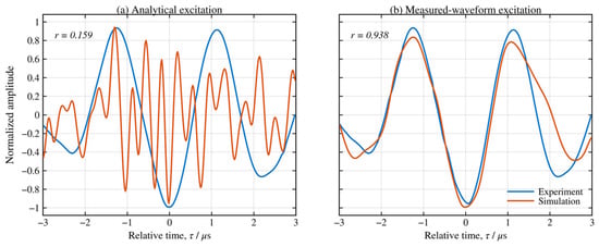
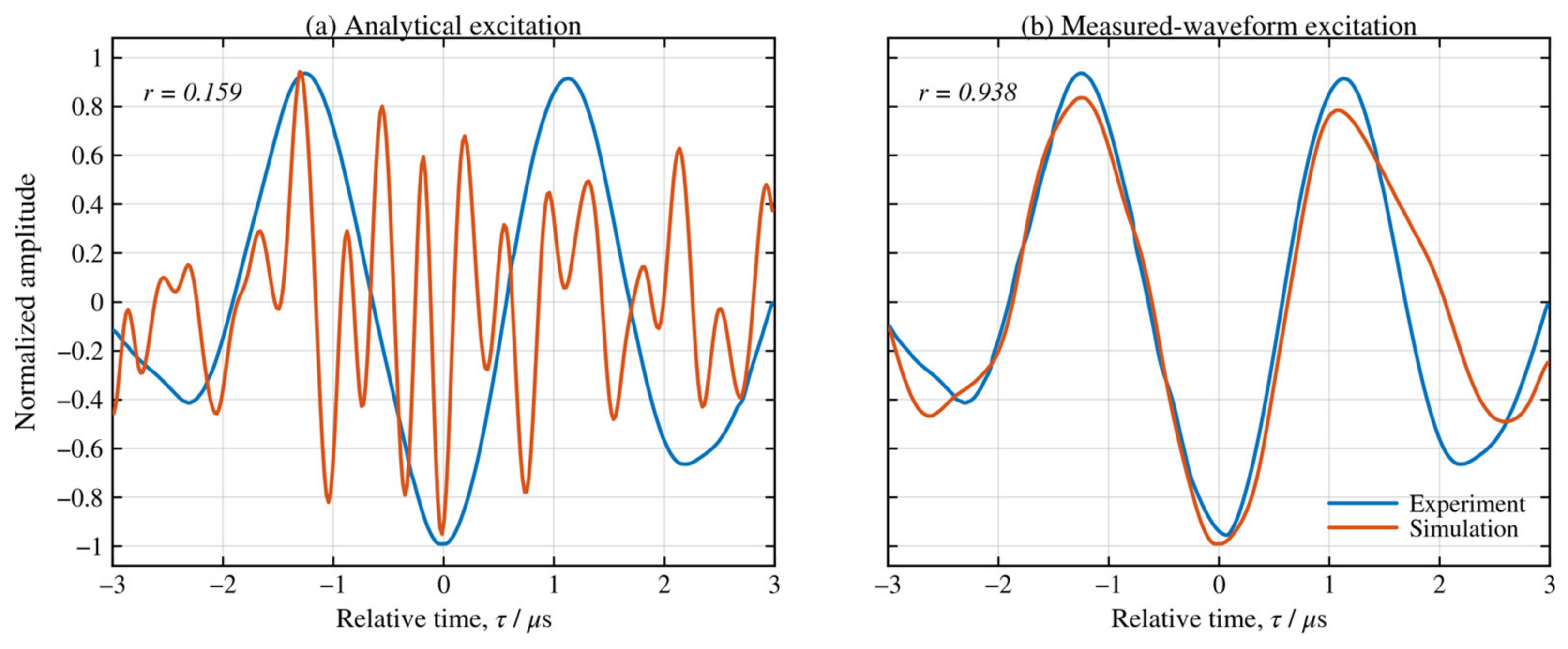
A transient excitation compatible with the experimental ultrasonic transducers was first required. The 300 kHz pulsed signal needed a defined dominant frequency and a finite duration and spatial extent. During initial model development, a sinusoidal pulse modulated by a Gaussian envelope was used as an idealized source. A smooth spatial weighting function was also applied over the transducer footprint. The resulting time–space expression was as follows:

$$g(t,s)=-\mathit{exp}[{\displaystyle \frac{{(t-t_p/2)}^2}{2{\sigma }^2}}]\mathit{sin}[2\pi f_0(t-t_p/2)]{\displaystyle \frac{1}{\sqrt{2\pi }}}\mathit{exp}[-{\displaystyle \frac{{(10s-5)}^2}{12}}]$$

(8)

Here, f₀ is the center frequency (300 kHz). The pulse center parameter and the associated envelope parameters control the pulse position and duration, while the spatial weighting describes a smooth distribution over a finite excitation region.

The analytical excitation was prescribed by a function and could not fully reproduce the actual wave packet formed by the transducers and receiving chain. The model therefore also used the measured reference waveform after consistent filtering and amplitude normalization. This waveform was imported into COMSOL as an interpolated time function, retaining its principal oscillations and envelope. Displacement or normal-acceleration amplitudes were specified separately through the corresponding boundary conditions.

The steel-plate responses obtained with the analytical excitation and measured reference waveform were compared. To examine local waveform changes, relative time was defined separately from the principal characteristic peak in the experiment and simulation. Normalized waveforms were compared within 3 μs before and after the peak. Propagation times were compared on the original time axes without peak alignment.

Figure 5 shows that the simulated wave packet obtained with the analytical excitation differed substantially from the experiment. With the measured reference waveform, the principal positive and negative extrema, oscillation period, and envelope became much closer to the experimental response. The local Pearson correlation coefficient increased from 0.159 to 0.938. Before alignment, the experimental and simulated characteristic peaks occurred at 14.81 and 16.20 μs, respectively, differing by 1.39 μs, mainly because of the specified material parameters. This comparison shows that the measured excitation improved reproduction of the wave packet shape and allowed subsequent material experiments and models to use a common waveform-processing procedure.

Figure 5. Experimental and numerical first-arrival responses in casing steel with different excitation waveforms.

2.3.2. Excitation Boundaries and Material Parameters

The filtered measured excitation signal s(t) was first normalized to a dimensionless time function:

$$f(t)={\displaystyle \frac{s\left(t\right)}{\mathit{max}\left|s\right(t\left)\right|}}$$

(9)

This procedure preserved the measured envelope, oscillation period, and phase. Solid displacement and fluid normal-acceleration excitations were then constructed according to the boundary conditions used in the solid mechanics and pressure acoustics models, respectively.

For solids, the mechanical vibration applied by the transducer to the specimen surface was represented by a prescribed-displacement boundary. The displacement along the propagation direction was written as follows:

u_x(t) = U₀f(t)

(10)

The displacement–amplitude scale was set to 1 nm. In the linear–elastic calculations, this common small-displacement scale allowed waveform responses in different materials to be compared under the same input conditions. It specified the computational excitation without changing the procedure for comparing separately normalized waveforms.

For fluids, a normal-acceleration boundary represented the mechanical drive applied by the transducer:

$$a_n(t)={\displaystyle \frac{d^{2}u\left(t\right)}{d{t}^2}}=U_0{\displaystyle \frac{d^{2}f\left(t\right)}{d{t}^2}}$$

(11)

Normal acceleration has units of m/s², and its time history was imported into COMSOL through an interpolation function. Solid displacement and fluid normal acceleration were applied to the corresponding physics interfaces using the same reference waveform-processing procedure.

Solids were modeled as isotropic linear–elastic materials, with density, Young’s modulus, and Poisson’s ratio specified for each specimen. Material dissipation was approximated using stiffness-proportional Rayleigh damping, with the mass-proportional term set to zero. The parameters are listed in Table 3. Damping coefficients were selected from available information and modeling experience. The analysis focused on propagation and interface effects under these prescribed material conditions. With the mass-proportional coefficient set to zero, the equivalent Rayleigh damping ratio at frequency f is ζ(f) = πfβ, where β is the stiffness-proportional coefficient. The Table 3 coefficients were prescribed for the laboratory specimens on the basis of material type, specimen condition, and modeling considerations.

Table 3. Material parameters used for the solid media in the numerical models.

Material	ρ/(kg·m−3)	E/GPa	ν	Stiffness Damping β/s	cL/(m·s−1)
AISI 4340 steel	7850	205	0.30	2.0 × 10−9	5929
Dry core	2360	30	0.20	1.0 × 10−8	3758
Water-saturated core	2400	33	0.25	1.6 × 10−8	4062
Dry cement	1900	13	0.22	1.3 × 10−8	2795
Water-saturated cement	2150	16	0.28	2.1 × 10−8	3084

Fluid acoustic properties were described mainly by density, sound speed, and viscosity. Air properties were used in the local-pore model of the rock core. The parameters are listed in Table 4.

Table 4. Material parameters used for the fluid media in the numerical models.

Medium	ρ/(kg·m−3)	c/(m·s−1)	Dynamic Viscosity/(Pa·s)	Bulk Viscosity/(Pa·s)
Clean water	1000	1500	0.001	0.0025
Impurity-containing water	1220	1560	0.020	0.050
Air	1.2	343	1.82 × 10−5	2.0 × 10−5

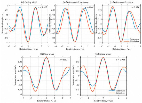
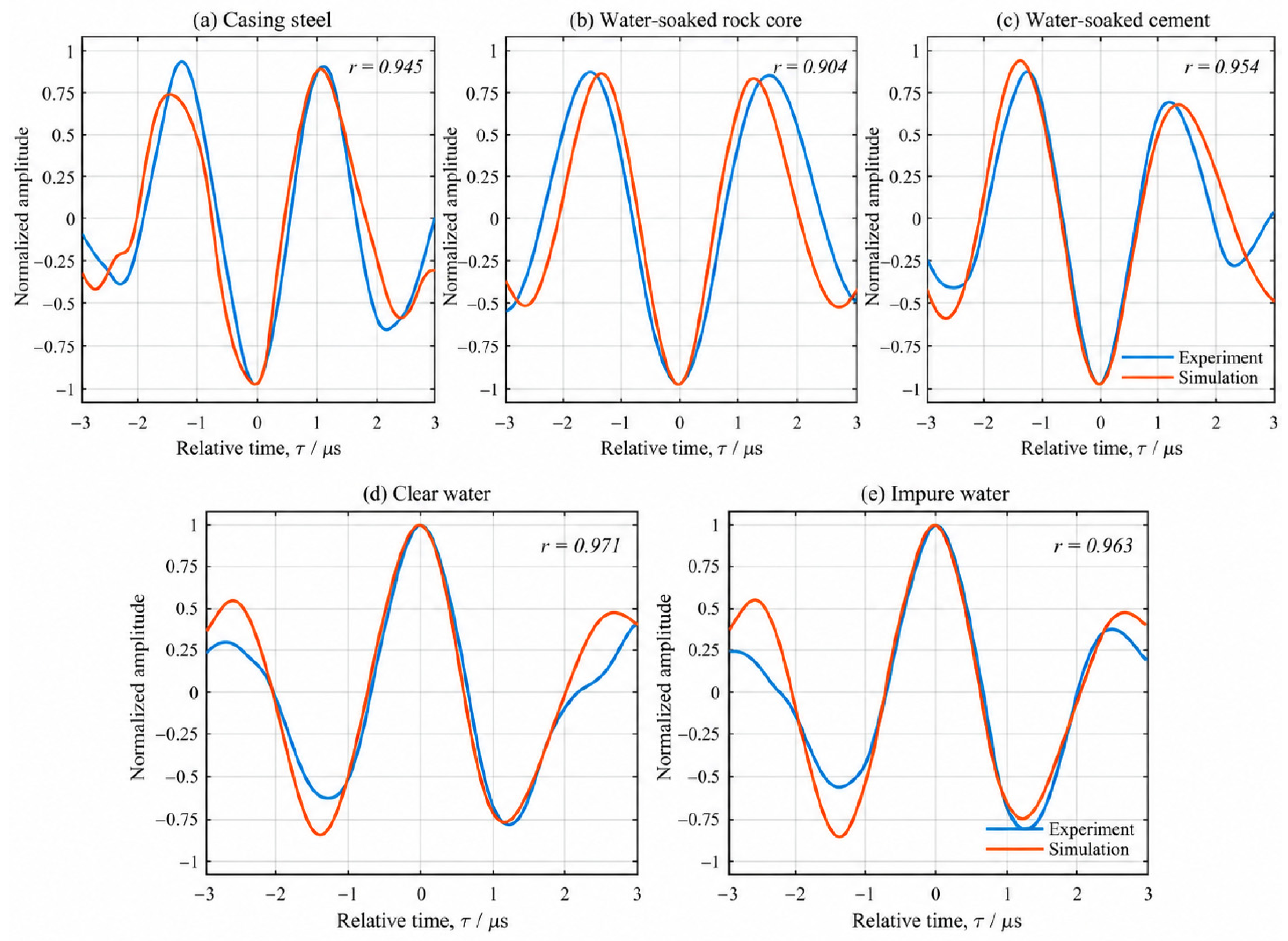
2.3.3. Comparison of Experimental and Numerical Waveforms

The experimental and simulated responses were compared in waveform shape and first-arrival peak amplitude to assess the model’s representation of propagation in different media. Each response was first normalized by its own maximum absolute amplitude within the first-arrival window. Relative time was defined from the main peak, and the principal extrema, oscillation period, and local envelope were compared within 3 μs on either side. Pearson correlation coefficients were also calculated. The results are shown in Figure 6.

Figure 6. Normalized experimental and numerical first-arrival waveforms in different media.

Figure 6 shows that the simulations reproduced the principal oscillatory structures of the transmitted wave packets in all five media. After main-peak alignment, the Pearson correlation coefficients ranged from 0.904 to 0.971. The measured excitation therefore enabled the models to reproduce the principal extrema, oscillation periods, and local waveform variations across the media. The locally normalized and peak-aligned Pearson coefficient evaluates waveform shape similarity but does not independently validate absolute amplitude, unaligned arrival time, or transmitted energy. These aspects are therefore considered separately through the original peak times, within-group relative peaks, and spectral comparisons.

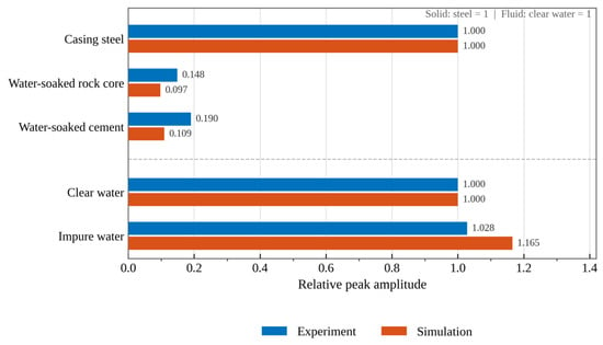
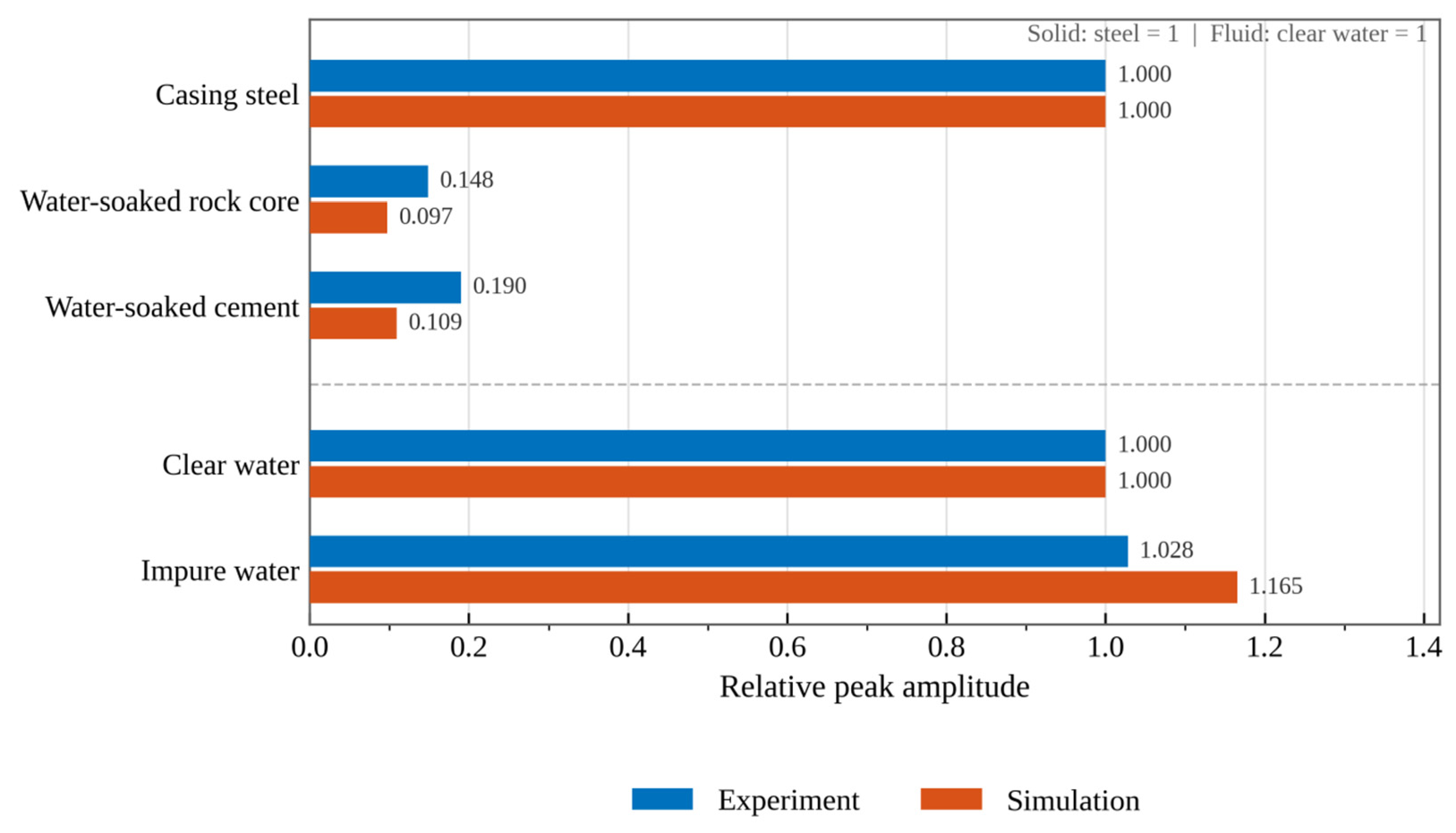
The maximum absolute amplitude within each first-arrival window was then extracted to compare relative transmission responses among the media in the experiments and simulations. The experiments recorded receiver voltage, whereas the simulations returned equivalent longitudinal-wave pressure in solids or acoustic pressure in fluids. Their absolute values were therefore not compared directly. Relative peaks were calculated separately within each dataset using the steel plate as the common solid reference and clean water as the common fluid reference. The results are shown in Figure 7.

Figure 7. Relative first-arrival peak amplitudes in different media from experiments and simulations.

Figure 7 shows that the steel plate produced the strongest solid-material response, with substantially lower peaks in the water-saturated core and cement. With the steel-plate peak set to 1, the experimental and simulated relative peaks were 0.148 and 0.097 for the water-saturated core, respectively. The corresponding values for water-saturated cement were 0.190 and 0.109. Both datasets showed higher peaks in steel than in water-saturated cement and slightly higher peaks in cement than in the water-saturated core. With clean water set to 1, the experimental and simulated relative peaks in impurity-containing water were 1.028 and 1.165, respectively. Both increased, but by different amounts. The model thus reproduced the principal ordering of relative response strengths for these materials, although the peak ratios did not agree exactly.

Before peak alignment, the experimental and simulated characteristic peak times differed by approximately 1.39–4.74 μs across the five individual media. These discrepancies may reflect material sound speed parameters, actual specimen conditions, and coupling. The model’s propagation response was assessed mainly through first-arrival wave packet shape and relative peak changes; peak times served as supporting information.

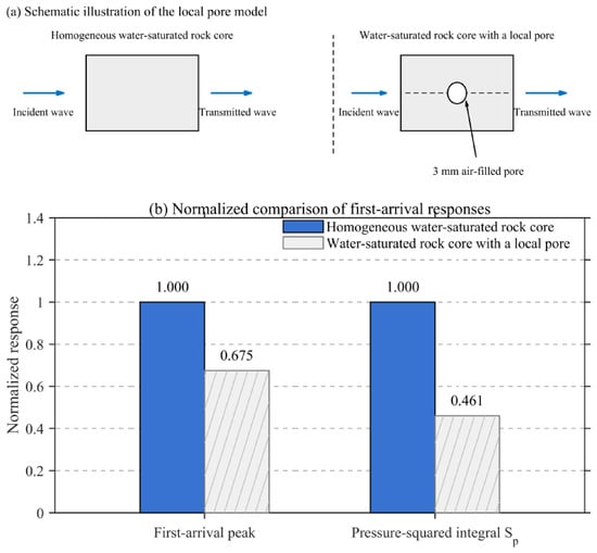
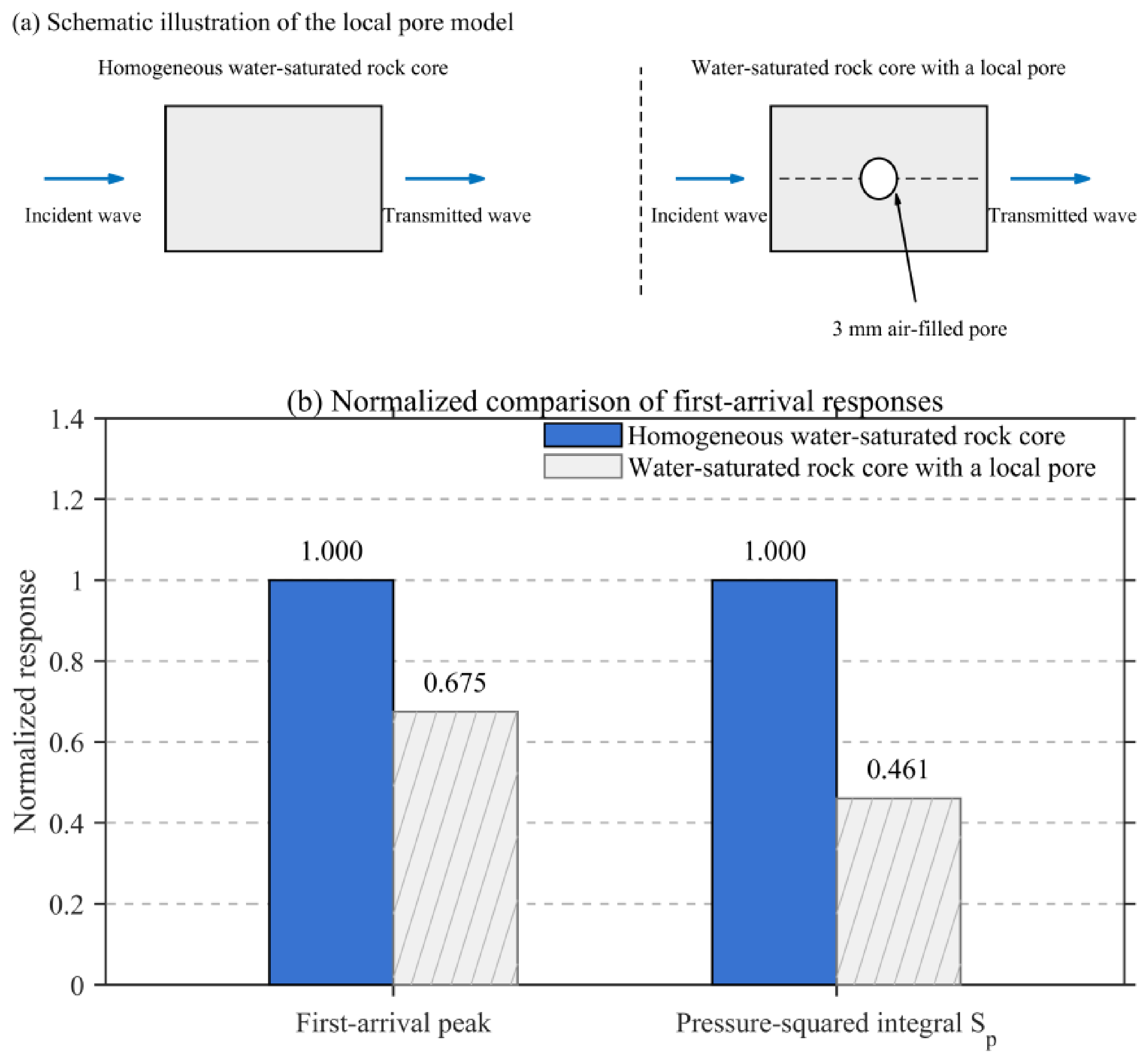
Following the material comparisons, homogeneous and local-pore models of the water-saturated core were used to examine propagation through a heterogeneous structure. A local air-filled pore was introduced, while all other parameters and the excitation were held constant. The principal transmitted wave packets were compared using the pressure-squared integral over the same time window as an auxiliary index:

$$S_p=\int p_{\mathit{eq}}^2\left(t\right)\mathit{dt}$$

(12)

This integral describes waveform intensity for the same physical quantity and time window; it is not directly equivalent to acoustic energy crossing a section. The comparison is shown in Figure 8.

Figure 8. Effect of a local air-filled pore on the principal transmitted response in a water-saturated core.

Figure 8 shows that introducing the local air-filled pore reduced the principal wave packet peak by approximately 32.5% and the pressure-squared integral by approximately 53.9% relative to the homogeneous model. The large impedance contrast between the air-filled pore and water-saturated rock matrix altered the local wavefield, weakening the response along the original receiver path. In addition to thickness, internal structure and interface differences can therefore substantially alter the local transmitted wave packet. This result supported further investigation of fluid–solid combinations.

Together, the waveform-shape and relative-peak comparisons show that the models driven by the measured excitation reproduced the principal transmitted wave packets in the individual media. They also captured the qualitative trends in relative response strength among the tested materials. These local experimental comparisons and pore-model results provided a basis for subsequent analysis of fluid–solid interfaces and stagewise attenuation in dual-string wells.

3. Experimental and Numerical Validation of Ultrasonic Transmission Across a Fluid–Solid Interface

A complete dual-string wellbore contains successive fluid–solid interfaces as well as different materials. A clean-water/steel-plate combination was therefore examined to determine the response changes after crossing a fluid–solid interface and provide an experimental reference for multilayer propagation.

3.1. Fluid–Solid Experiment and Numerical Model

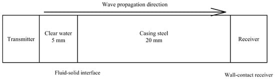
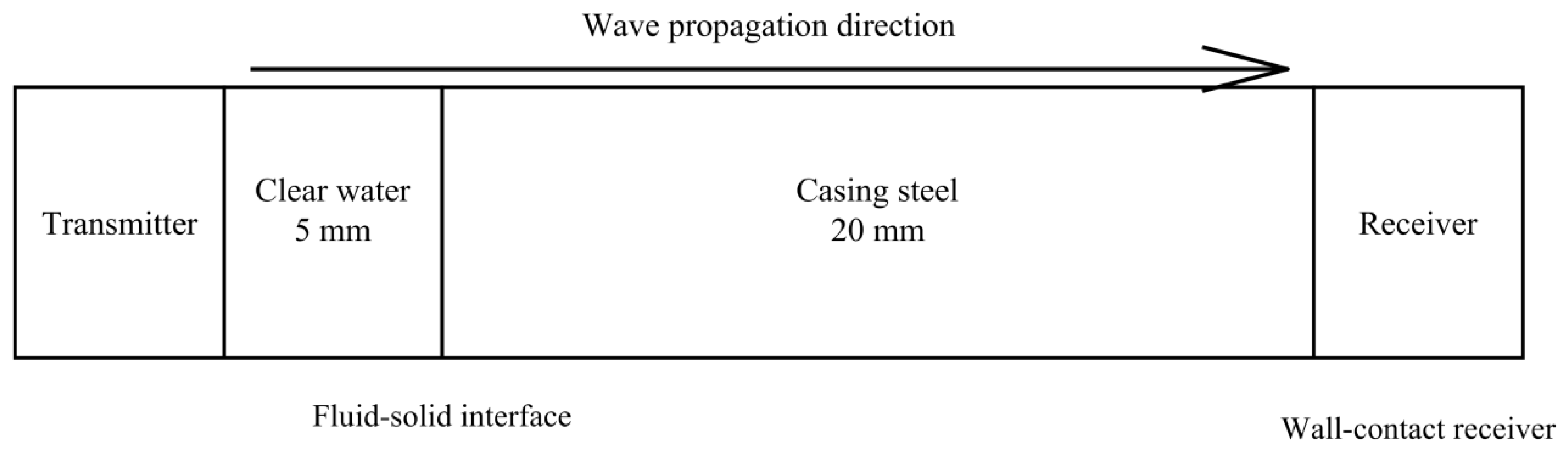
The original test system and excitation-processing procedure were retained. A 5 mm clean-water layer was placed before a 20 mm steel plate, with the receiving transducer attached to the outer steel surface. The model used the same layer sequence and thicknesses. Pressure acoustics and solid mechanics jointly described transmission near the water–steel interface. The specimen arrangement and propagation direction are shown in Figure 9.

Figure 9. Equivalent propagation paths in the combined-structure experiment and numerical model.

Clean water and steel differ substantially in acoustic impedance, causing both reflection and transmission when a wave reaches their interface. An ideal planar interface with a normally incident plane wave was first used as a theoretical reference. Acoustic impedance was defined from material density and longitudinal-wave velocity:

Z = ρc

(13)

Here, ρ and c are material density and longitudinal-wave velocity, respectively. Under ideal normal incidence, the energy partition into the transmitted wave can be expressed as follows:

$$T_I={\displaystyle \frac{4Z_w{Z}_s}{{(Z_w+Z_s)}^2}}$$

(14)

The densities and sound speeds of clean water and steel give acoustic impedances of approximately 1.50 and 46.54 MRayl, respectively. The corresponding ideal normal-incidence energy transmission coefficient is approximately 0.121. Interfaces between high- and low-impedance materials therefore strongly affect transmitted acoustic energy. The actual response is also influenced by finite layer thickness, multiple reflections, transducer frequency response, and coupling conditions.

3.2. Time- and Frequency-Domain Comparison Between Experiment and Simulation

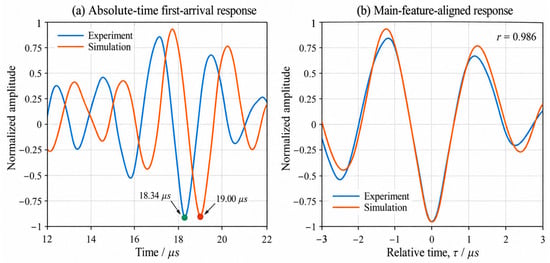
Using the material sound speeds specified in the model, the calculated transit time through 5 mm of clean water and 20 mm of steel was approximately 6.71 μs. The principal characteristic peak of the direct reference waveform occurred near 12.1 μs, giving an estimated transmitted wave packet arrival near 18.81 μs for the combined structure. The experimental and simulated peaks occurred at 18.34 and 19.00 μs, respectively, both close to this estimate. The selected packets therefore had a physically reasonable correspondence in propagation time.

Figure 10 shows similar wave packet shapes, sequences of extrema, and oscillation periods in the water–steel experiment and simulation. Before alignment, the characteristic peaks occurred at 18.34 and 19.00 μs, respectively, differing by 0.66 μs. After normalization and main-peak alignment, the local Pearson correlation coefficient was 0.986. Together with the theoretical transit time through 5 mm of water and 20 mm of steel, these results indicate that the model reproduced the principal transmitted packet’s time-domain characteristics. They provide local experimental support for subsequent analysis of successive fluid–solid interfaces.

Figure 10. Experimental and numerical first-arrival waveforms for the combined structure.

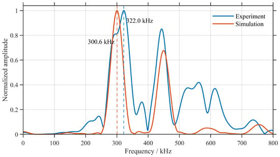
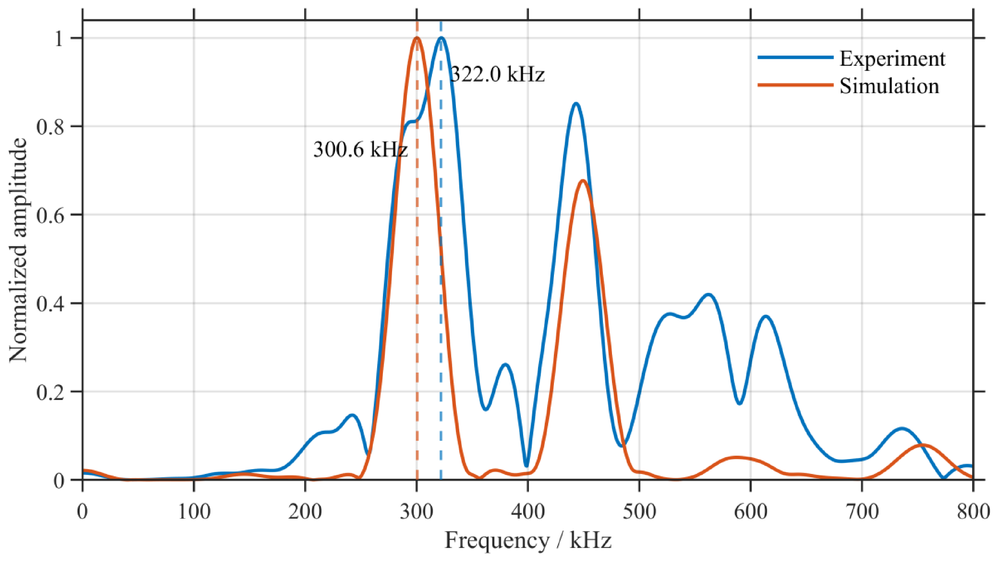
To assess preservation of the received signal’s frequency content, the effective experimental and simulated responses from 10 to 60 μs were extracted for a windowed Fourier transform. Each spectrum was normalized by its own maximum. The comparison is shown in Figure 11.

Figure 11. Normalized experimental and numerical received-signal spectra for the combined structure.

Figure 11 shows dominant experimental and simulated peaks at 322.0 and 300.6 kHz, respectively, both within the principal operating band of the 300 kHz transducer. Although the experimental spectrum contained richer high-frequency components, the dominant frequencies and representative oscillatory features corresponded. Combined with the time-domain results, this agreement indicates that the model reasonably described the principal cross-interface response near the operating frequency used here.

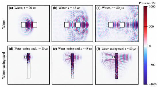
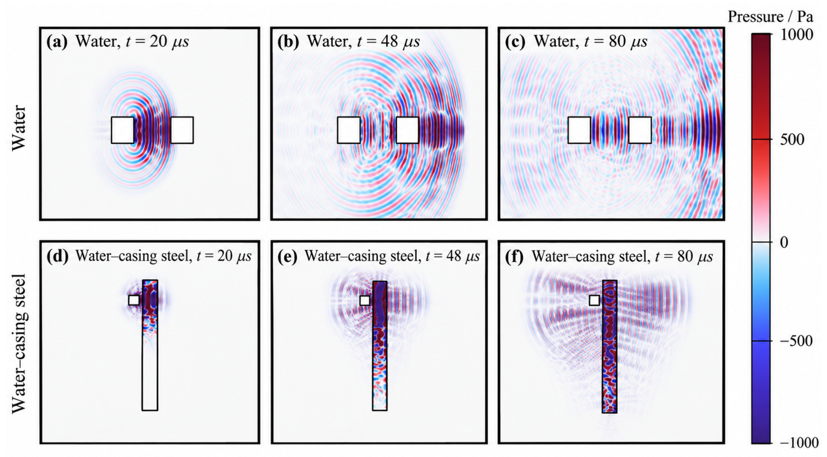
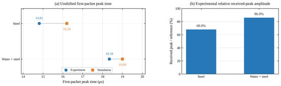
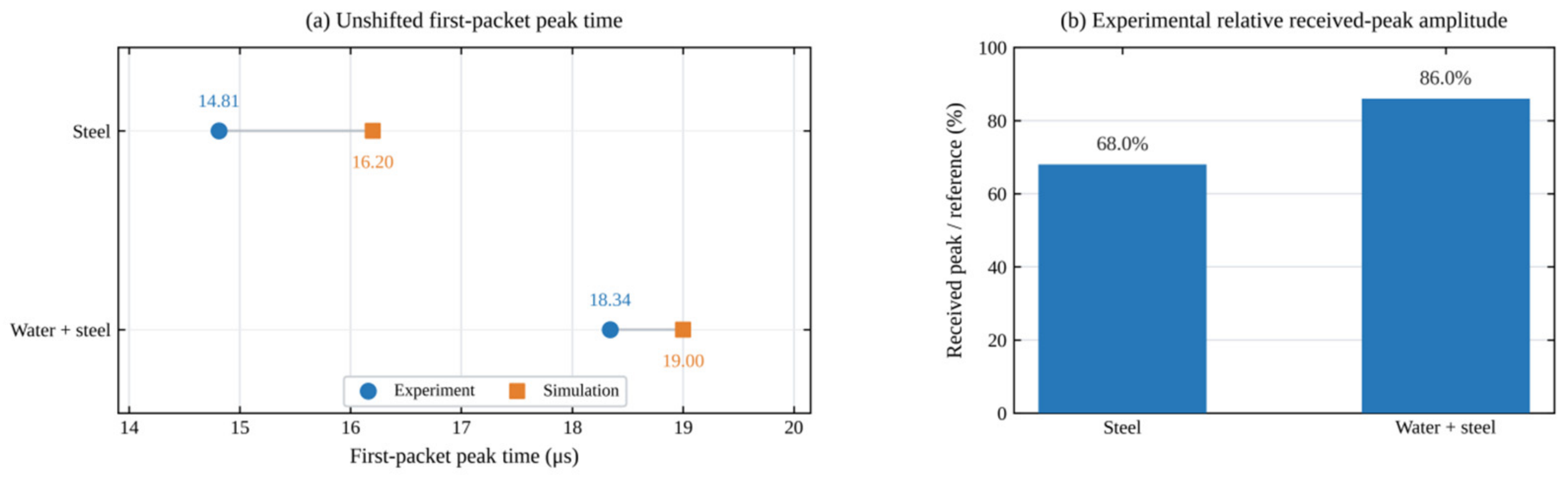
Figure 12 compares propagation in clean water and the water–steel combination. The packet propagated relatively directly in clean water. Introducing the steel plate caused pronounced reflection near the water–steel interface, while a transmitted wave still crossed the steel and reached the receiver side. Together with the received wave packet changes in Figure 10, these observations show that fluid–solid transmission altered both response strength and wave packet structure. Figure 13 further compares characteristic peak times and received peak amplitudes for steel alone and the water–steel combination using common reference conditions.

Figure 12. Wavefield propagation in clean water and the water–steel combination corresponding to the local experiments.

Figure 13. Characteristic peak times and relative experimental received amplitudes for steel alone and the water–steel combination.

Figure 13a compares characteristic peak times for steel alone and the water–steel combination on the original time axes. For steel alone, the experimental and simulated peaks occurred at 14.81 and 16.20 μs, respectively. For the water–steel combination, they occurred at 18.34 and 19.00 μs. Adding the water layer delayed the experimental and simulated peaks by 3.53 and 2.80 μs, respectively. Both therefore showed a later arrival of the principal transmitted wave packet. The experimental–numerical peak time difference for the water–steel combination was 0.66 μs, approximately 0.2 periods at 300 kHz. Figure 10 also shows similar principal extrema and a Pearson correlation coefficient of 0.986, while both dominant frequencies in Figure 11 are near 300 kHz. Together, these comparisons show good correspondence between experiment and simulation in the principal transmitted waveform, propagation timing, and frequency characteristics. Figure 13b compares the experimental received peaks under the same reference conditions. The peaks were 147.44 mV for steel alone and 186.47 mV for the water–steel combination, or 68.0% and 86.0% of the direct reference peak, respectively. Adding the water–steel interface therefore did not simply reduce the local received peak. Instead, the peak reflected the combined effects of interface reflection and transmission, wave packet superposition, and coupling. Changes in received peak amplitude cannot be equated directly with interface energy transmittance and require interpretation alongside propagation characteristics.

The individual–medium and water–steel comparisons assessed the model’s representation of the principal ultrasonic transmission characteristics. Experiments and simulations corresponded well in waveform shape, dominant frequency, and characteristic peak time, indicating a reasonable description of propagation in individual media and across a local fluid–solid interface. A complete path through wellbore fluid, tubing, annular fluid, casing, cement, and formation is more complex. Reflections, transmissions, and superposed wave packets make the effects of individual layers and interfaces difficult to distinguish from the final received signal alone. A complete dual-string wellbore model was therefore needed to analyze stagewise radial propagation by interface decomposition and examine the effects of individual layers and interfaces on overall attenuation.

4. Interface Decomposition and Attenuation Prediction for Multilayer Propagation in an Ideal Dual-String Wellbore

4.1. Axisymmetric Dual-String Wellbore Model and Interface-Decomposition Method

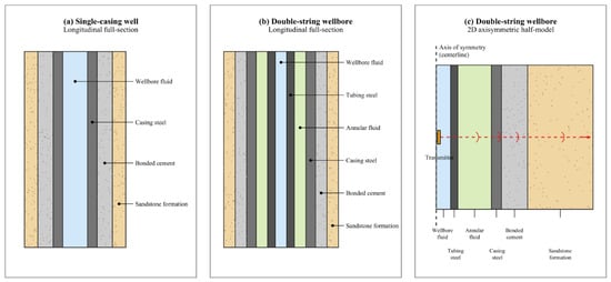
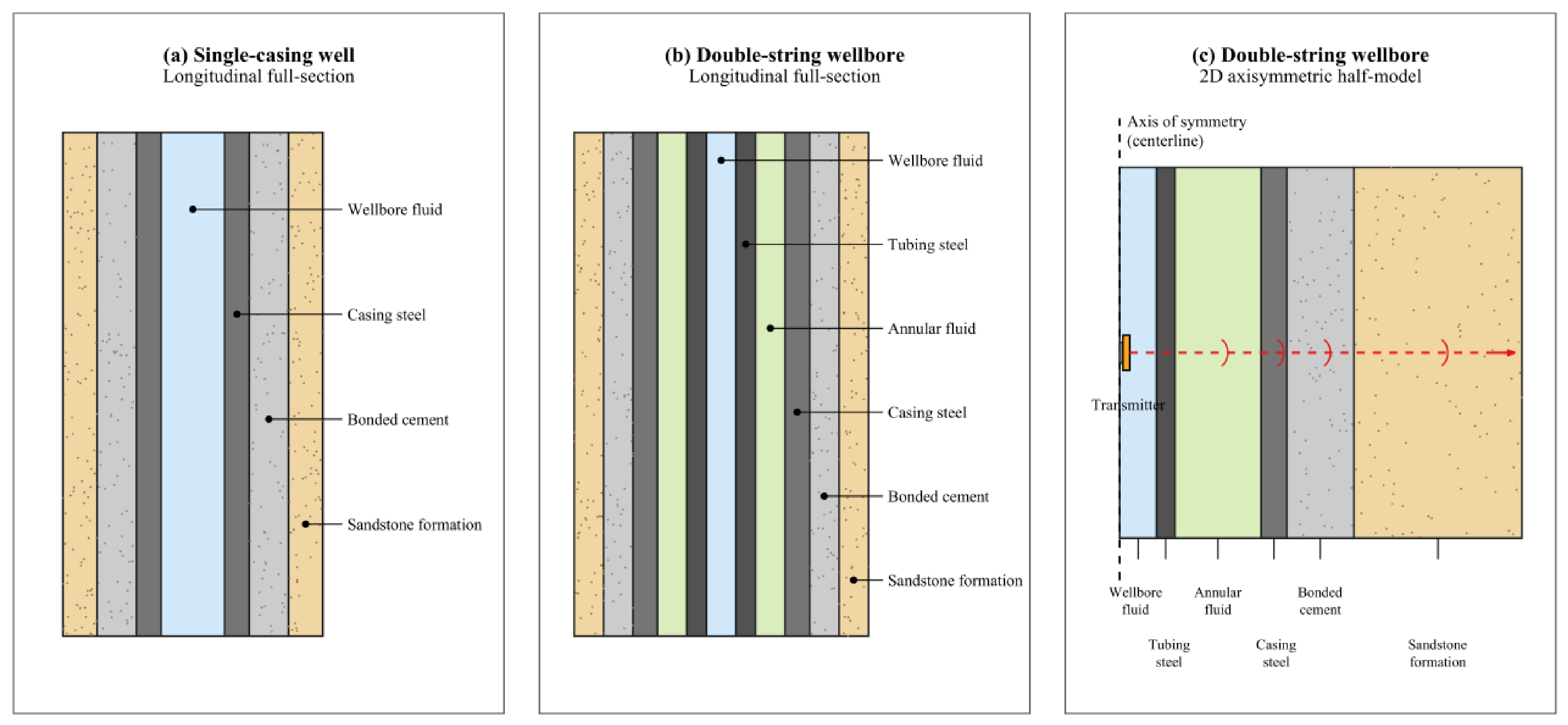
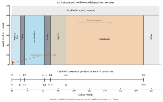
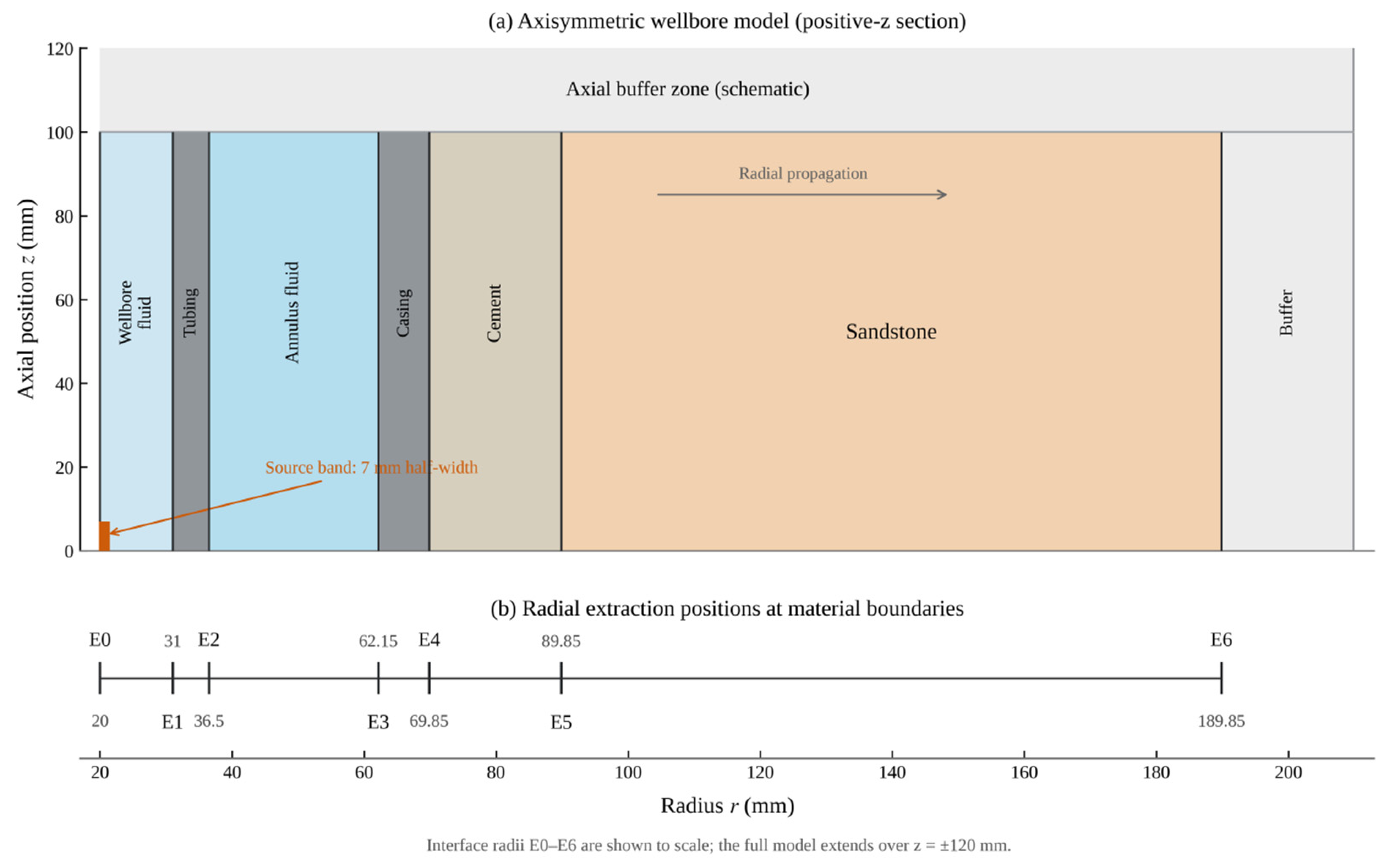
For individual media and the water–steel combination, received experimental packets could be related relatively directly to their propagation paths. In an actual dual-string wellbore, tubing, annular fluid, casing, cement sheath, and formation form successive layers whose interfaces jointly affect the final received waveform. An ideal concentric dual-string wellbore was therefore represented by a two-dimensional axisymmetric model, with successive radial extraction positions at the material-layer boundaries. The axisymmetric formulation assumes ideal concentric layers and a circumferentially uniform equivalent excitation. It does not represent tool eccentricity, azimuthally localized transducer radiation, or other circumferentially non-uniform features; these effects require three-dimensional modeling. The layer sequence and probe arrangement are shown in Figure 14 and Figure 15, respectively.

Figure 14. Single-casing and dual-string wellbore structures and radial material-layer sequences.

Figure 15. Two-dimensional axisymmetric domain and successive radial probes for the ideal concentric dual-string wellbore (dimensions in mm).

From the inside outward, the model comprised 11 mm of wellbore fluid, 5.5 mm of tubing steel, 25.65 mm of annular fluid, 7.7 mm of casing steel, 20 mm of well cement, and 100 mm of sandstone. The excitation reference surface was at a radius of 20 mm, and the axial domain extended over z = ±120 mm. Seven radial nodes, E0–E6, were located at 20, 31, 36.5, 62.15, 69.85, 89.85, and 189.85 mm. Each adjacent pair enclosed one material layer. The six stages through wellbore fluid, tubing, annular fluid, casing, cement, and sandstone could therefore be analyzed successively.

Transient pressure acoustics were used for fluids and solid mechanics for the steel strings, cement, and formation, with acoustic-structure coupling at fluid–solid interfaces. A circumferentially uniform equivalent axisymmetric excitation used the processed measured reference waveform. Radiation and low-reflecting conditions were applied at the external fluid and solid boundaries, respectively. The stiffness-proportional Rayleigh damping coefficients for steel, cement, and sandstone were 2.5 × 10⁻⁹, 1.3 × 10⁻⁸, and 8 × 10⁻⁹ s, respectively. The mass-proportional term was zero. Unlike the specimen-specific coefficients in Table 3, these values are prescribed engineering-equivalent settings for the ideal wellbore materials, reflecting different material assumptions and modeling purposes. These values defined the prescribed material conditions. The principal wave packet peak amplitude Ai and outward work Wi were used to characterize local packet responses and overall outward energy transfer during radial propagation.

The principal wave packet envelope peak at radial node i within its analysis window was defined as follows:

$$A_i=\underset{t\in {\mathcal{T}}_i}{\mathit{max}}\left|q_i\left(t\right)+j\hspace{0.17em}\mathcal{H}\left[q_i\left(t\right)\right]\right|$$

(15)

Here, q_i(t) is the extracted fluid acoustic pressure or effective solid normal traction at radial node i, $\mathscr{H}$ denotes the Hilbert transform, and $𝒯$_i is the corresponding principal wave packet analysis window.

For the numerical sensitivity comparisons, the packet extraction procedure was revised after inspection of the complete original time histories. The Hilbert envelope was calculated from the full 0–120 μs record. On reference mesh A, the earliest local maximum within 3.3–90 μs satisfying a height threshold of 25% and a prominence threshold of 3% of the reference maximum, with a minimum peak separation of 0.6 μs, was used as the node-specific anchor. A fixed window extending one 300 kHz period (3.333 μs) on each side of that anchor was then applied identically to all meshes and time steps. The envelope maximum within this window represents an early composite response, not an independently isolated first-arrival mode. No waveform time alignment or gain adjustment was used for the sensitivity comparisons.

The peak-amplitude loss between adjacent nodes was defined as follows:

$$L_{i-1\to i}^{\left(A\right)}=20{\mathit{log}}_{10}\left({\displaystyle \frac{A_{i-1}}{A_i}}\right)$$

(16)

To further examine radial wave transfer, outward work across each radial section was calculated over the same observation period:

$$W_i={\int }_0^{120\hspace{0.17em}\mathit{\mu s}}{\int }_{S_i}\mathit{max}\left[P_{r,i}\left(z,t\right),\hspace{0.17em}0\right]\hspace{0.17em}\mathit{dS}\hspace{0.17em}\mathit{dt}$$

(17)

Here, P_r,i(z,t) is the instantaneous radial power flux density across section i, and S_i is its actual integration region. The outward radial direction was taken as positive. Power flux was calculated from acoustic pressure and radial velocity in fluids and from effective stress and the corresponding velocity components in solids:

$$P_{r,i}\left(z,t\right)=\left\{\begin{array}{ll}p\hspace{0.17em}{v}_r,& \mathit{fluid},\\ -\left({\sigma }_{\mathit{rr}}^{\mathit{eff}}{v}_r+{\sigma }_{\mathit{rz}}^{\mathit{eff}}{v}_z\right),& \mathit{solid}.\end{array}\right.$$

(18)

For the two-dimensional axisymmetric model, the section-area element was

dS = 2πr_i dz

(19)

where r_i is the section radius; v_r and v_z are radial and axial velocities; and ${\mathsf{\sigma }}_{\mathrm{rr}}^{\mathrm{eff}}$ and ${\mathsf{\sigma }}_{\mathrm{rz}}^{\mathrm{eff}}$ are effective solid stress components. Every section was integrated over the same 0–120 μs period and its actual spatial extent in the model. The term max(P_r,i,0) accumulates local positive power flux; the resulting work is not the network obtained by canceling positive and negative contributions. The common 0–120 μs interval includes the selected early response at E6 (approximately 70.275 μs) and part of the subsequent superposed field. Because cumulative outward work at E6 still increases by approximately 35.9% from 110 to 120 μs, this interval defines a finite observation window rather than an all-time energy convergence limit.

The outward-work loss between adjacent nodes was defined as follows:

$$L_{i-1\to i}^{\left(W\right)}=10{\mathit{log}}_{10}\left({\displaystyle \frac{W_{i-1}}{W_i}}\right)$$

(20)

A positive loss indicates weakening over that stage, whereas a negative value indicates local enhancement.

4.2. Radial Propagation and Stagewise Attenuation in the Dual-String Wellbore

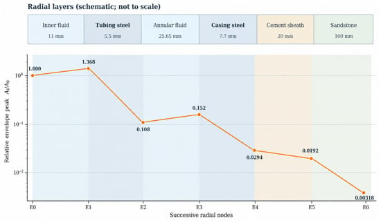
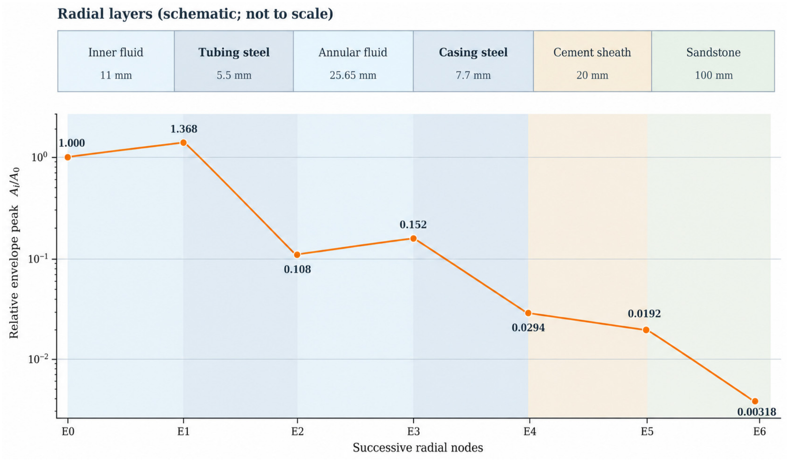
Figure 16 shows principal wave packet amplitudes at radial nodes E0–E6. Local amplitude did not decrease continuously as ultrasound propagated outward. It increased near the inner tubing surface and within the annular fluid but decreased substantially after crossing the two steel strings. Individual layers therefore affected the response differently. Propagation distance or the final amplitude alone could not capture the changes near interfaces.

Figure 16. Relative early composite response envelope peaks at successive radial nodes in the dual-string wellbore.

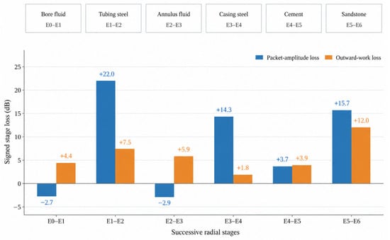
To relate these observations to the structure, amplitude changes were calculated for the six stages between adjacent nodes and compared with outward work across the sections. The results are shown in Figure 17. The following analysis examines the principal responses around the two steel strings and their physical origins.

Figure 17. Signed envelope-peak losses of the early composite response and cumulative outward-work losses over 0–120 μs across six successive propagation stages in the ideal dual-string wellbore.

Figure 16 and Figure 17 show that the early-response envelope peak increased from approximately 2.89 to 3.95 kPa over E0–E1 but fell to approximately 0.313 kPa at E2 after crossing the tubing steel. It increased again to approximately 0.438 kPa at E3 at the outer edge of the annular fluid before falling to approximately 0.085 kPa at E4 after crossing the casing. Local early responses could therefore increase within the wellbore and annular fluids, while the selected response weakened substantially across the tubing and casing. The stagewise differences were concentrated near the steel layers rather than distributed uniformly along the radial path.

Over E0–E1, from the wellbore fluid toward the tubing, the steel wall and fluid had a large contrast in acoustic impedance. The incident wave traveling toward the steel and the reflected wave returning into the fluid altered the near-interface pressure distribution, potentially producing a large local peak. After the wave crossed the tubing and reached the outer fluid, elastic propagation in the steel, reflections at both interfaces, and fluid–solid conversion jointly altered the packet. The principal peak consequently fell markedly over E1–E2. Although the first-arrival envelope peak recovered over E2–E3 in the annular fluid, it remained substantially below the amplitude at E1 inside the tubing. This local increase therefore did not compensate for the preceding amplitude loss.

The stagewise amplitude changes in Figure 17 show local peak enhancement over E0–E1 and E2–E3 within the revised common early-response windows. The corresponding amplitude losses were approximately −2.72 and −2.93 dB. By contrast, losses across the tubing (E1–E2) and casing (E3–E4) were approximately 22.02 and 14.25 dB, respectively; the cement and sandstone stages showed losses of approximately 3.69 and 15.65 dB. These stagewise values describe differences between prescribed adjacent observation sections and include both propagation within each enclosed layer and interactions at its interfaces.

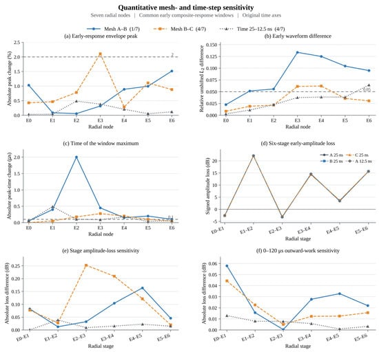
Figure 18 presents quantitative mesh and time step sensitivity results using the revised common early-response windows. Three meshes with prescribed maximum/minimum sizes of 0.7/0.14, 0.5/0.10, and 0.35/0.07 mm were compared with the same controlled 25 ns time integration setting; an independent comparison on mesh A used 25 and 12.5 ns. The largest change in a single stage’s amplitude loss was 0.2525 dB for mesh refinement and 0.0389 dB for time step refinement; the corresponding maximum outward-work loss differences were 0.0443 and 0.0129 dB. The revised common-window definition changed the tubing-stage estimate from 26.51 to 22.02 dB without changing the underlying COMSOL field solution. The signs of all six stage-amplitude changes were preserved, although complete nodal or joint space–time convergence was not demonstrated.

Figure 18. Quantitative mesh and time step sensitivity of early composite responses at seven radial nodes and six successive propagation stages in the dual-string wellbore.

A supplementary check on the finest mesh examined sampling sections 0.5 and 1.0 mm inside both steel layers, using like-sided solid-response quantities. For the tubing, the early-envelope loss changed from 22.018 dB across the full layer to 6.928 and 3.545 dB for the two shortened interior spans; the corresponding casing values were 14.306, 5.679, and −0.319 dB. The matched cumulative outward-work losses remained positive. Moving both sampling sections also shortens the propagation path and changes near-interface interference; therefore, these differences represent section-dependent responses, not pure probe-placement error or intrinsic steel attenuation.

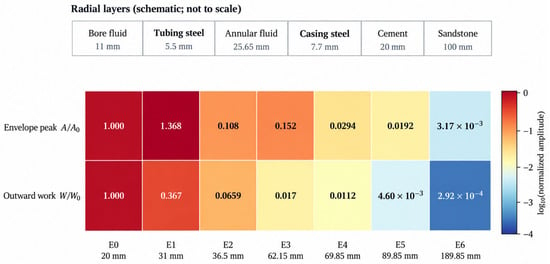
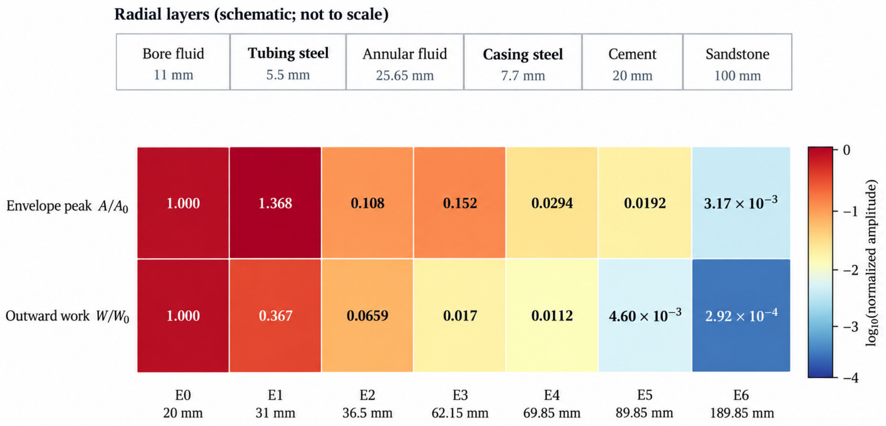
Figure 19 compares principal wave packet amplitudes and outward work across radial sections, each normalized to its value at E0. Local peaks and outward work did not change in parallel. For example, the early-response peak increased by approximately 36.8% over E0–E1, whereas 0–120 μs cumulative outward work at E1 was approximately 36.7% of that at E0 over the selected period. A large local peak therefore did not necessarily mean that a comparable amount of wave motion continued outward. Point amplitudes and section responses must be considered together when interpreting the complete propagation path.

Figure 19. Relative early-response envelope peaks and cumulative outward work over 0–120 μs at successive radial nodes, normalized to their respective E0 values.

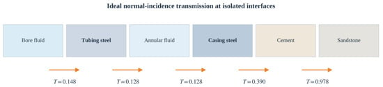
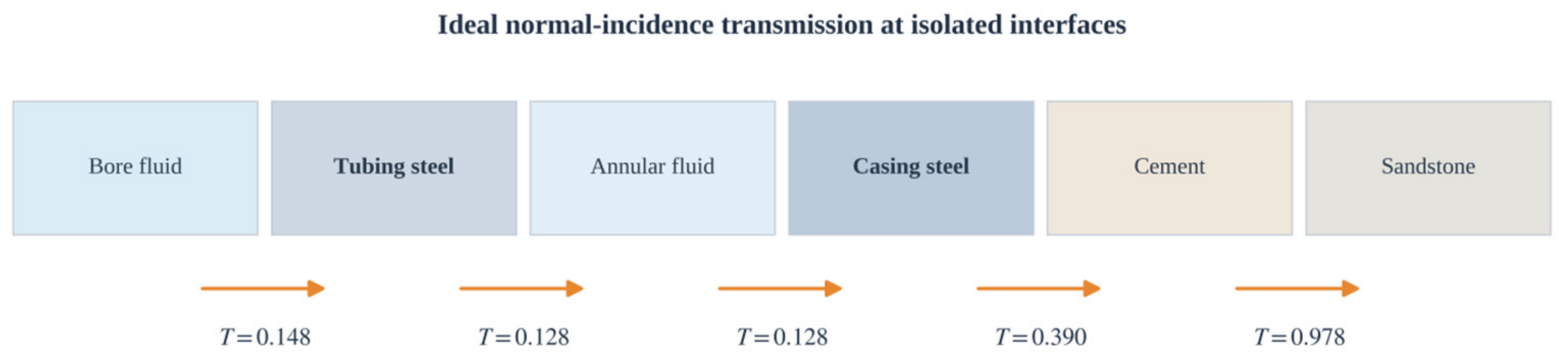
These differences can be further understood through material acoustic impedances and interfacial wave interactions. The wellbore fluid, steel strings, and annular fluid differ substantially in impedance. Figure 20 lists ideal plane-wave normal-incidence transmission coefficients at adjacent interfaces as a theoretical reference. When a wave reaches high-impedance steel from a low-impedance fluid, reflection changes the local pressure, while transmission conditions control the portion continuing outward. Upon entry into fluid or cement, impedance contrasts and propagation within the steel jointly affect the outer packet. Although both steel layers caused clear amplitude changes, they should not be treated as two identical attenuation units.

Figure 20. Theoretical energy transmission coefficients at adjacent interfaces in the dual-string wellbore under ideal normal incidence.

The tubing mainly separates two fluids, whereas the casing is bounded externally by well cement. Even with the same steel, different neighboring media change reflection and transmission conditions. The local packets around the tubing and casing therefore undergo different amplitude losses. After crossing the tubing, the effective packet entering the annulus is already much weaker than the inner response. The casing and cement act on this weaker input and further reduce the identifiable outer packet. This sequence is an important reason that the effects of multiple media accumulate in a dual-string wellbore.

Figure 17 and Figure 19 show that local peak changes and outward-work changes convey different physical information. Local amplitude increased over E0–E1, while outward work decreased. A local amplitude recovery was also observed over E2–E3. Enhanced local reflections can therefore increase peaks at individual observation points without indicating that more wave motion has reached the outer layers. Both indices are needed to describe the local response and wave transfer across sections separately.

Across the six stages, the two steel strings and nearby interfaces produced pronounced changes in the principal transmitted packet. The cement and formation continued to affect the already attenuated outer response. Under the ideal concentric geometry and prescribed excitation considered here, the early composite-response envelope peak at E6 was approximately 0.32% of that at E0. The modeled outer response was therefore much weaker than the inner response. Successive stagewise extraction also identified the layers that jointly contributed to the overall weak outer signal.

5. Conclusions

This study combined 300 kHz material transmission experiments, a water–steel experiment, and numerical simulations of an ideal concentric wellbore. Ultrasonic responses were extracted stage by stage along a multilayer path to examine how different materials and fluid–solid interfaces affected the outer wave packet. The following conclusions were obtained.

(1)

The individual-medium experiments and corresponding models showed good agreement in principal with wave packet shape. The measured reference excitation increased the local correlation coefficient for steel from 0.159 to 0.938. For the water–steel combination, experimental and simulated peak times differed by 0.66 μs before alignment, and the principal operating frequencies were both near 300 kHz. These results provide specific local experimental support for modeling propagation within materials and across a fluid–solid interface.

(2)

In the ideal concentric dual-string model, the layers affected wave packets differently. Local peak enhancement occurred near the wellbore and annular fluids, whereas the selected early composite-response peaks weakened substantially after crossing the tubing and casing. Changes near the two steel strings were particularly pronounced among the six stages. Interface decomposition related these observations to specific material layers.

(3)

Local wave packet amplitude and outward work across a section did not change in parallel. A large local pressure peak may arise from reflection and near-interface wavefield changes and does not necessarily indicate greater outward transmission. By progressing from individual media and local combinations to a complete wellbore, the study resolved propagation stages that are difficult to distinguish from the final signal in a multilayer string structure. The results provide numerical evidence for the formation of weak outer-layer signals in an ideal intact dual-string wellbore and provide a reference for further studies of interface effects under complex field conditions.

Several limitations should be noted. The ideal axisymmetric model excludes eccentric tools, azimuthally localized sources, and non-uniform circumferential structures. Rayleigh damping was prescribed rather than independently calibrated from frequency-dependent attenuation, and the complete dual-string model has not been directly validated by a full-string physical experiment. Future work will pursue controlled full-well experiments, independently constrained material parameters, further numerical convergence checks, and three-dimensional analyses of eccentricity, non-uniform cement bonding, and interface defects.

References

- Zhang, C.; Luo, L.; Shao, Y.; Ma, Z.; Duan, S. Research progress and engineering applications of carbon capture, utilization and storage technology. Petrol. Geol. Recovery Effic. 2026, 33, 243–254. [Google Scholar] [CrossRef]
- Zhang, M.; Bachu, S. Review of integrity of existing wells in relation to CO2 geological storage: What do we know? Int. J. Greenh. Gas Control 2011, 5, 826–840. [Google Scholar] [CrossRef] [Scilit]
- Bai, M.; Zhang, Z.; Fu, X. A review on well integrity issues for CO2 geological storage and enhanced gas recovery. Renew. Sustain. Energy Rev. 2016, 59, 920–926. [Google Scholar] [CrossRef] [Scilit]
- Carroll, S.; Carey, J.W.; Dzombak, D.; Huerta, N.J.; Li, L.; Richard, T.; Um, W.; Walsh, S.D.C.; Zhang, L. Review: Role of chemistry, mechanics, and transport on well integrity in CO2 storage environments. Int. J. Greenh. Gas Control 2016, 49, 149–160. [Google Scholar] [CrossRef] [Scilit]
- Teodoriu, C.; Bello, O. A review of cement testing apparatus and methods under CO2 environment and their impact on well integrity prediction—Where do we stand? J. Pet. Sci. Eng. 2020, 187, 106736. [Google Scholar] [CrossRef] [Scilit]
- Kruszewski, M.; Montegrossi, G.; Ramírez Montes, M.; Wittig, V.; Gomez Garcia, A.; Sánchez Luviano, M.; Bracke, R. A wellbore cement sheath damage prediction model with the integration of acoustic wellbore measurements. Geothermics 2019, 80, 195–207. [Google Scholar] [CrossRef] [Scilit]
- Wang, H.; Tao, G.; Shang, X. Understanding acoustic methods for cement bond logging. J. Acoust. Soc. Am. 2016, 139, 2407–2416. [Google Scholar] [CrossRef] [Scilit] [PubMed]
- Zeroug, S.; Bose, S.; Sinha, B.K.; Skataric, M.; Liu, Y.; D’Angelo, R. Sonic and ultrasonic measurement applications for cased oil wells. Insight Non-Destr. Test. Cond. Monit. 2016, 58, 423–430. [Google Scholar] [CrossRef] [Scilit]
- Tang, J.; Zhang, C.; Zhang, B.; Shi, F. Cement bond quality evaluation based on acoustic variable density logging. Pet. Explor. Dev. 2016, 43, 514–521. [Google Scholar] [CrossRef] [Scilit]
- Tang, X.M.; Jiang, C.; Su, Y.D.; Chen, X.L. An acoustic-wave theory for casing bond evaluation using viscoelastic slip boundary modeling. Sci. China Earth Sci. 2018, 61, 1057–1064. [Google Scholar] [CrossRef] [Scilit]
- Jiang, C.; Chen, X.L.; Su, Y.D.; Tang, X.M. Cased borehole acoustic-wave propagation with varying bonding conditions: Theoretical and experimental modeling. Geophysics 2019, 84, D161–D169. [Google Scholar] [CrossRef] [Scilit]
- He, X.; Chen, H.; Wang, X. Ultrasonic leaky flexural waves in multilayered media: Cement bond detection for cased wellbores. Geophysics 2014, 79, A7–A11. [Google Scholar] [CrossRef] [Scilit]
- Xu, F.; Hu, H. Inversion of the shear velocity of the cement in cased borehole through ultrasonic flexural waves. Geophysics 2017, 82, D57–D68. [Google Scholar] [CrossRef] [Scilit]
- Liu, Y.; D’Angelo, R.M.; Sinha, B.K.; Zeroug, S. Theoretical and experimental investigations of acoustic waves in embedded fluid-solid multi-string structures. Appl. Phys. Lett. 2017, 110, 101906. [Google Scholar] [CrossRef] [Scilit]
- Viggen, E.M.; Johansen, T.F.; Merciu, I.A. Simulation and modeling of ultrasonic pitch-catch through-tubing logging. Geophysics 2016, 81, D383–D393. [Google Scholar] [CrossRef] [Scilit]
- Viggen, E.M.; Johansen, T.F.; Merciu, I.A. Analysis of outer-casing echoes in simulations of ultrasonic pulse-echo through-tubing logging. Geophysics 2016, 81, D679–D685. [Google Scholar] [CrossRef] [Scilit]
- Viggen, E.M.; Johansen, T.F.; Merciu, I.A. Simulation and inversion of ultrasonic pitch-catch through-tubing well logging with an array of receivers. NDT E Int. 2017, 85, 72–75. [Google Scholar] [CrossRef] [Scilit]
- Talberg, A.S.; Johansen, T.F.; Larsen, I. Laboratory experiments on ultrasonic logging through casing for barrier integrity validation. In Proceedings of the ASME 2017 36th International Conference on Ocean, Offshore and Arctic Engineering, Trondheim, Norway, 25–30 June 2017. Paper OMAE2017-62645. [Google Scholar] [CrossRef] [Scilit]
- Liu, Y.; D’Angelo, R.M.; Choi, G.; Zhu, L.; Patel, M.; Bose, S.; Zeroug, S.; Merciu, I.A.; Constable, K. Experimental investigation of acoustic features associated with cement damages in double cased-wellbores. AIP Conf. Proc. 2019, 2102, 050024. [Google Scholar] [CrossRef] [Scilit]
- Correia, T.M.; Souza, L.P.B.; Hidalgo, J.A.S.; Ribeiro, M.G.C.; Camerini, I.G.; Sousa, B.G.; Kubrusly, A.C.; Ayala, H.V.H.; Batista, J.H.G.; Almeida, R.V. Analytical and numerical modeling of through-tubing acoustic logging. In Proceedings of the Rio Oil & Gas Expo and Conference, Rio de Janeiro, Brazil, 21–24 September 2020. Article 099. [Google Scholar] [CrossRef] [Scilit]
- Chen, X.L.; Jiang, C.; Zhuang, C.X.; Tang, X.M. Response characteristics of monopole sonic log in double casing strings. Chin. J. Geophys. 2020, 63, 4268–4276. [Google Scholar] [CrossRef]
- Chen, X.L.; Tang, X.M. The wavefield characteristics of dipole acoustic logging in a double-casing well. Chin. J. Geophys. 2021, 64, 363–371. [Google Scholar] [CrossRef]
- Chen, D.; Yin, Y.; Zhang, C.; Chen, S.; Guan, W. Ultrasonic Lamb wave detection of a channel in a double-casing well. Ultrasonics 2023, 130, 106916. [Google Scholar] [CrossRef] [Scilit] [PubMed]
- de Souza, L.P.B.; Ferreira, G.R.B.; Camerini, I.G.; Correia, T.M.; Ribeiro, M.G.C.; Hidalgo, J.A.S.; de São João, B.L.D.; Angulo Llerena, R.W.; Kubrusly, A.C.; Ayala, H.V.H.; et al. Machine learning-based cement integrity evaluation with a through-tubing logging experimental setup. Geoenergy Sci. Eng. 2023, 227, 211882. [Google Scholar] [CrossRef] [Scilit]
- Zhang, S.; Zeng, Z.; Wang, X.; Chen, S.; Liu, Y. Imaging in double-casing wells with convolutional neural network based on inception module. APL Mach. Learn. 2024, 2, 026105. [Google Scholar] [CrossRef] [Scilit]
- de Souza, L.P.B.; Hidalgo, J.A.S.; Correia, T.M.; Camerini, I.G.; Ferreira, G.R.B.; Rodrigues, A.S.; Kubrusly, A.C.; Braga, A.M.B. Acoustic wave propagation in oil wells: A comparison between semi-analytical and finite element modeling approaches. Wave Motion 2025, 134, 103487. [Google Scholar] [CrossRef] [Scilit]
- Ji, Y.; Huang, J.; Wang, H.; Bi, Q.; Shi, S.; Gu, Y. Full-wave decomposition and mode wave analysis of through-tubing monopole acoustic logging. IEEE Trans. Geosci. Remote Sens. 2025, 63, 5900910. [Google Scholar] [CrossRef] [Scilit]
- Evident Scientific. Material Sound Velocities. Ultrasonic Thickness Gauge Tutorial. Available online: https://ims.evidentscientific.com/en/learn/ndt-tutorials/thickness-gauge/appendices-velocities (accessed on 23 October 2026).
- Kassab, M.A.; Weller, A. Study on P-wave and S-wave velocity in dry and wet sandstones of Tushka region, Egypt. Egypt. J. Pet. 2015, 24, 1–11. [Google Scholar] [CrossRef] [Scilit]
- Zheng, Y.; Liu, C.; Lu, K.; Zhang, H.; Jian, B.; Zhang, W. Study on the fracture behavior and critical slowing down characteristics of saturated sandstone based on acoustic emission and resistivity. Sci. Rep. 2025, 15, 12113. [Google Scholar] [CrossRef] [Scilit] [PubMed]
Disclaimer/Publisher’s Note: The statements, opinions and data contained in all publications are solely those of the individual author(s) and contributor(s) and not of MDPI and/or the editor(s). MDPI and/or the editor(s) disclaim responsibility for any injury to people or property resulting from any ideas, methods, instructions or products referred to in the content. |
© 2026 by the authors. Licensee MDPI, Basel, Switzerland. This article is an open access article distributed under the terms and conditions of the Creative Commons Attribution (CC BY) license.