Machine Learning-Based Rapid Seismic Damage Evaluation for Concrete Arch Dams

Abstract

A fast and accurate assessment of earthquake-induced damage in arch dams is critical for emergency management, yet conventional approaches, such as field investigations, numerical simulations, and fragility-based assessments, are inadequate for timely and reliable damage evaluation. This study proposes a rapid seismic damage state assessment framework for arch dams based on machine learning techniques. Feature screening, machine learning algorithm selection, and hyperparameter optimization are systematically incorporated to develop prediction models with strong generalization capability. The proposed methodology is demonstrated through a case study of a high arch dam in southwestern China. A total of 1000 dynamic simulations are performed to generate a ground motion intensity measure-seismic damage state dataset for model training and testing. By considering five feature scenarios and employing six machine learning algorithms, 30 candidate machine learning models are developed and evaluated. Among all the developed prediction models, the ANN model under the 20-feature scenario achieves the best overall predictive performance, with an overall accuracy of 0.88. The trained model can be deployed in earthquake alert systems to rapidly evaluate the seismic damage state of arch dams using monitored ground motion data, thereby facilitating emergency decision-making.

1. Introduction

Concrete arch dams are a common type of massive water-retaining structure. A fast and accurate assessment of earthquake-induced damage to arch dams is crucial for the emergency management operations of dams (such as flood discharge, dam reinforcement, and the evacuation of downstream residents). Conventional methods used to determine the post-earthquake damage state of arch dams include on-site investigations, numerical simulations using recorded ground motions, and estimation from seismic fragility curves. On-site investigations require trained engineers to visually inspect the condition of the dam and determine whether it is safe. Such investigations are time-consuming and labor-intensive. Similarly, nonlinear time-history analysis is also time-consuming and cannot satisfy the efficiency requirements because of its heavy modeling and computational workload for a three-dimensional arch dam–foundation system. Fragility estimation can only provide the probability of exceeding a given damage state and cannot explicitly predict the damage state itself. Moreover, current seismic fragility analyses of arch dams typically rely on a single ground motion intensity measure, peak ground acceleration (PGA) [1,2]. Such a single intensity measure cannot adequately capture the complex time-frequency characteristics of ground motions, thereby limiting the accuracy of fragility estimates [3]. In summary, these traditional approaches cannot meet the requirements for timely and accurate seismic damage assessment. Recently, machine learning and its applications in various research fields have attracted considerable attention [4,5,6,7]. Prediction models developed using machine learning algorithms have emerged as a promising approach for the fast and accurate assessment of seismic damage.

Rapid seismic damage assessment based on machine learning has been extensively investigated for building and bridge structures. Xu et al. [8] applied three different machine learning algorithms (support vector machine, logistic regression, and decision tree) to develop seismic damage prediction models for an individual building and regional building clusters. The models were evaluated using accuracy and F1-score, which are commonly used metrics for classification tasks. The results demonstrated that the developed models were reliable for seismic damage prediction in buildings. Mangalathu et al. [9] developed prediction models for the seismic damage states of bridge portfolios using various machine learning algorithms. The input variables of these models included not only seismic intensity measures but also various bridge design attributes. The best-performing model selected from the candidate models was integrated into earthquake alert systems to rapidly assess the damage states of bridges given a new set of input parameters. Similar research approaches and findings are also reported in the literature [10,11,12,13,14,15]. The results of these studies demonstrate that machine learning-based damage assessment methods can satisfy the requirements for rapid and accurate post-earthquake damage state identification. However, as massive concrete structures, the seismic behavior of arch dams differs significantly from that of buildings and bridges. The application of machine learning-based damage assessment methods to arch dams still requires further investigation.

Machine learning methods have been used in research on performance-based earthquake engineering for concrete dams. Hariri-Ardebili and Sasan Barak [16] were among the first to apply machine learning algorithms to the prediction of the seismic responses of gravity dams. They discussed the application of six different machine learning techniques to forecasting the structural displacement and stress responses of gravity dams under earthquakes and demonstrated the applicability of machine learning algorithms. Subsequently, Hariri-Ardebili et al. [17] further extended the application of machine learning algorithms to the prediction of the seismic responses of arch dams, including crest displacement, maximum body stress, and nodal stresses throughout the entire dam. Both real and synthetic ground motion records were used to construct the dataset, and five scenarios were defined using separate and mixed groups of real and synthetic ground motions. The predictive capability of the machine learning-based metamodels was systematically evaluated, and the results indicated that the kernel extreme learning machine outperformed the other machine learning methods. Segura et al. [18,19] identified the most suitable metamodel for seismic fragility assessment of gravity dams. Specifically, a comparative analysis of six metamodeling techniques was performed to determine the best-performing regression metamodel for predicting the base sliding of gravity dams. Li et al. [20] trained a BP neural network-based surrogate model for the seismic failure analysis of gravity dams, and its predictive performance was validated. The established surrogate model was then used to predict the damage states of gravity dams under a large number of seismic ground motions, thereby reducing the computational cost of nonlinear earthquake analysis in seismic risk assessment. The aforementioned studies mainly employed regression-based supervised machine learning algorithms to predict the seismic responses of dams, such as displacement, stress, and sliding. In contrast, the present study aims to predict the seismic damage states of dams, which requires the use of classification-based supervised learning algorithms.

This paper proposes a new methodology for the rapid seismic damage state assessment of arch dams by utilizing the capabilities of machine learning algorithms. The proposed method consists of training and deploying the prediction model during the pre-earthquake stage, followed by predicting the damage state of arch dams during the post-earthquake stage using features extracted from monitored ground motion records. The core of this approach lies in constructing a machine learning model with strong generalization capability. Consequently, the key techniques involved in model development, including feature selection, the choice of machine learning algorithms, and the optimization of model hyperparameters, are carefully taken into consideration to enhance the predictive accuracy of the model. The proposed method is applied to a real arch dam located in the seismically active region of southwestern China to verify its feasibility.

The rest of the paper is organized as follows: In Section 2, six different machine learning classification algorithms considered in this study are briefly reviewed. Section 3 illustrates the proposed framework for rapid seismic damage assessment in detail. Description and modeling, damage state criteria, and ground motion selection of the case study arch dam are provided in Section 4. In Section 5, the proposed methodology is applied to the case study arch dam, and the detailed treatments in dataset generation and training and test of machine learning models are discussed. Section 6 summarizes the major findings and presents directions for future work.

2. A Brief Overview of Machine Learning Classification Techniques

In this study, seismic damage state prediction models for arch dams are developed using machine learning classification techniques, enabling rapid post-earthquake damage assessment. Six various classification algorithms, i.e., Logistic Regression (LR), Decision Tree (DT), K-Nearest Neighbors (KNN), Support Vector Machine (SVM), Artificial Neural Networks (ANN), and Random Forest (RF), are explored in the current study. These algorithms are briefly reviewed in this section for engineers who are not familiar with the fundamentals of classification algorithms, and interested readers are directed to References [21,22] for more detailed explanations.

2.1. Logistic Regression

Despite its name, Logistic regression (LR) is a linear model for classification rather than regression problems. The logistic regression is also known in the literature as logit regression, maximum-entropy classification or the log-linear classifier. Unlike linear regression, which predicts continuous variables, LR estimates the probability that a sample belongs to a particular class.

For binary classification problems, the relationship between the input variables and the output probability is established through the logistic function [23]:

$$p(y=1|\mathbf{x})={\displaystyle \frac{1}{1+\exp \left(-({\mathbf{w}}^{\mathrm{T}}\mathbf{x}+b)\right)}}$$

(1)

where $\mathbf{x}$ denotes the input feature vector, $\mathbf{w}$ represents the model weights, and b is the bias term. The output of the logistic function ranges from 0 to 1, which can be interpreted as the posterior probability of the sample belonging to the positive class. The model parameters are commonly estimated by maximizing the likelihood function or equivalently minimizing the cross-entropy loss function:

$$L=-{\displaystyle \frac{1}{N}}{\displaystyle \sum _{i=1}^N}\left[y_i\ln \left(p_i\right)+(1-y_i)\ln (1-p_i)\right]$$

(2)

where N is the number of training samples, $y_i$ is the true label, and $p_i$ is the predicted probability for the i-th sample. Optimization algorithms such as gradient descent method and Newton method are typically employed to determine the optimal parameters.

For multiclass classification problems, logistic regression can be extended using strategies such as one-versus-rest or multinomial logistic regression with the softmax function [24].

2.2. Decision Tree

Decision tree (DT) is a supervised machine learning algorithm widely used for classification and regression tasks due to its interpretability, simple implementation, and capability of handling nonlinear relationships and mixed data types. The fundamental principle of DT is to recursively partition the input feature space into several homogeneous subsets according to specific decision rules. The resulting model has a tree-like structure consisting of a root node, internal decision nodes, and leaf nodes [25].

In classification problems, the algorithm starts from the root node containing the entire training dataset and iteratively selects the optimal feature to split the data. The objective is to maximize the homogeneity of samples within each subset while increasing the separability among different classes. The selection of the splitting feature is typically based on impurity measures, such as information gain, gain ratio, or Gini impurity. Information gain is commonly adopted to evaluate the effectiveness of a feature split [26]:

$$IG(D,A)=Ent\left(D\right)-\sum _{v\in Values\left(A\right)}{\displaystyle \frac{|D_v|}{\left|D\right|}}Ent\left(D_v\right)$$

(3)

where D is the dataset, A represents the candidate feature, $D_v$ denotes the subset corresponding to a specific feature value, and $Ent\left(D\right)$ is the information entropy and can be expressed as:

$$Ent\left(D\right)=-{\displaystyle \sum _{i=1}^C}{p}_i{\log }_2{p}_i$$

(4)

where $p_i$ denotes the probability of samples belonging to class i, and C is the total number of classes. DT are prone to overfitting, especially when the tree becomes excessively deep. Therefore, pruning strategies are commonly employed to improve the generalization performance of the model. The final prediction is obtained by traversing the tree from the root node to a leaf node according to the feature values of an input sample.

2.3. K-Nearest Neighbors

The K-nearest neighbors (KNN) algorithm is a non-parametric supervised learning method [27]. In KNN, the classification of a new observation is determined based on the majority class among its K nearest neighbors in the feature space. Typically, a distance metric (e.g., Euclidean distance) is used to identify the nearest neighbors. A useful technique is to assign weights to the neighbors, such that closer neighbors exert a greater influence than more distant ones [28].

The conditional probability that an observation $\mathbf{x}$ belongs to class t can be estimated as:

$$P(Y=t\mid X=\mathbf{x})={\displaystyle \frac{1}{K}}\sum _{i\in N_K\left(\mathbf{x}\right)}I(y_i=t)$$

(5)

where $N_K\left(\mathbf{x}\right)$ denotes the set of K nearest neighbors of $\mathbf{x}$ in the training dataset, and $I(·)$ is the indicator function. The KNN classifier assigns the observation $\mathbf{x}$ to the class with the highest estimated probability. The optimal choice of K depends on the characteristics of the dataset. In general, larger values of K reduce the influence of noise on the classification results but tend to produce less distinct decision boundaries between classes. An appropriate value of K can be determined through hyperparameter optimization.

2.4. Support Vector Machine

Because of its strong generalization ability, robustness in high-dimensional spaces, and effectiveness with limited training samples, Support vector machine (SVM) has been extensively applied in classification tasks. The fundamental objective of SVM is to determine an optimal hyperplane that maximizes the margin between different classes in the feature space [29,30].

For linearly separable data, the optimization problem can be formulated as:

$$\begin{array}{cc}\hfill \underset{\mathbf{w},b}{\min }& {\displaystyle \frac{1}{2}}{\parallel \mathbf{w}\parallel }^2\hfill \\ \hfill \mathrm{s}.\mathrm{t}.& y_i({\mathbf{w}}^{\mathrm{T}}{\mathbf{x}}_i+b)\ge 1,i=1,2,\dots ,N\hfill \end{array}$$

(6)

where $\mathbf{w}$ and b are the weight vector and bias term, respectively, ${\mathbf{x}}_i$ and $y_i\in \{-1,+1\}$ denote the input feature vector and class label of the i-th sample, respectively, and N is the number of training samples. In practical applications, the data are often not linearly separable, and the optimal hyperplane is determined by maximizing the geometric margin while simultaneously minimizing classification errors. Soft-margin SVM is commonly adopted by introducing slack variables and a penalty parameter C to balance the trade-off between margin maximization and classification error minimization. For nonlinear classification problems, SVM employs kernel functions to map the original data into a higher-dimensional feature space, where linear separation becomes feasible [31]. Commonly used kernel functions include the linear kernel, polynomial kernel, radial basis function (RBF) kernel, and sigmoid kernel. Among them, the RBF kernel is frequently applied due to its strong capability in handling nonlinear relationships. SVM can be extended to multiclass classification problems through one-versus-rest or one-versus-one strategy.

2.5. Artificial Neural Networks

An artificial neural network (ANN) is a data-driven computational model inspired by the structure and information processing mechanism of biological neural systems. In classification tasks, ANNs aim to establish a nonlinear mapping relationship between the input features and the target categories through hierarchical feature learning [32].

A typical ANN consists of an input layer, one or more hidden layers, and an output layer. Each layer contains multiple artificial neurons. For a neuron in the hidden or output layer, the weighted sum of the inputs is first computed and then transformed through a nonlinear activation function such as the sigmoid, hyperbolic tangent, or rectified linear unit (ReLU) function. The forward propagation process can be expressed as:

$$z_j^{\left(l\right)}=\sum _i{w}_{ij}^{\left(l\right)}{a}_i^{(l-1)}+b_j^{\left(l\right)},a_j^{\left(l\right)}=f\left(z_j^{\left(l\right)}\right)$$

(7)

where $w_{ij}^{\left(l\right)}$ and $b_j^{\left(l\right)}$ denote the weight and bias parameters, respectively, $a_i^{(l-1)}$ represents the output from the previous layer, and $f(·)$ is the activation function.

For multiclass classification problems, the output layer commonly employs the Softmax activation function to convert the network outputs into posterior probabilities for each class:

$$P(y=k\mid x)={\displaystyle \frac{e^{z_k}}{{\sum }_{j=1}^K{e}^{z_j}}}$$

(8)

where K is the total number of classes and $z_k$ is the output of the k-th neuron in the output layer.

During the training process, the network parameters are optimized by minimizing a predefined loss function using gradient-based optimization algorithms. For classification tasks, the cross-entropy loss function is widely adopted:

$$L=-{\displaystyle \sum _{i=1}^N}{\displaystyle \sum _{k=1}^K}{y}_{ik}\log \left({\widehat{y}}_{ik}\right)$$

(9)

where N is the number of training samples, $y_{ik}$ is the true label, and ${\widehat{y}}_{ik}$ is the predicted probability for class k. The gradients of the loss function with respect to the network parameters are computed using the backpropagation algorithm, and the parameters are iteratively updated through optimization methods such as stochastic gradient descent or Adam.

2.6. Random Forest

Random Forest (RF) is an ensemble learning algorithm that combines multiple decision trees to improve the predictive accuracy and robustness of machine learning models [33]. The core principle of RF is based on the ensemble strategy of bagging (Bootstrap Aggregating) [34], in which a large number of decision trees are independently constructed using randomly sampled subsets of the training data and features.

For classification tasks, RF generates multiple bootstrap samples from the original training dataset through random sampling with replacement. Each decision tree is trained using one bootstrap sample, while a random subset of features is selected at each node during the splitting process. This feature randomness reduces the correlation among individual trees and enhances the diversity of the ensemble model. After all decision trees are constructed, the final classification result is determined through majority voting among the outputs of individual trees. Compared with a single decision tree, RF exhibits superior generalization capability and resistance to overfitting due to the averaging effect of multiple trees.

3. Proposed Rapid Seismic Damage Evaluation Framework for Arch Dams

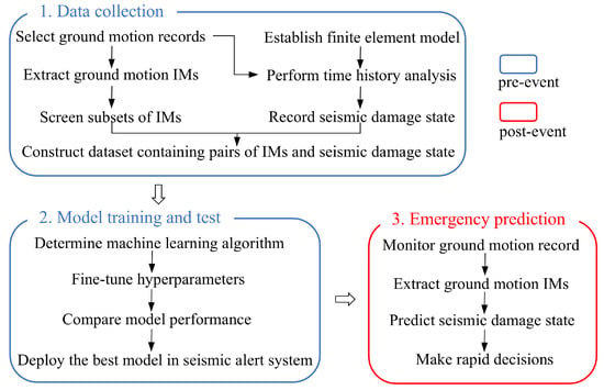
Utilizing the capabilities of machine learning algorithms to learn the mapping relationship between ground motion intensity measures (IMs) and structural damage states, a methodology for rapidly classifying the damage state of arch dams into one of the three levels (i.e., no damage, moderate damage, or severe damage) after an earthquake is proposed in this section. The proposed framework is divided into two main parts: (1) the pre-event process and (2) the post-event process.

To get ready for the near-real-time damage assessment in times of emergency, the pre-event process should be performed first. The pre-event process has the following two steps:

• Step 1: Data collection. According to the engineering site conditions, appropriate real ground motions are selected from a ground motion database. The IMs of these ground motions are then computed and used as features in the dataset. It is noteworthy that many IMs exhibit strong correlations, and using a large number of highly correlated IMs may lead to information redundancy, thereby reducing the predictive performance of the model. Therefore, the screening of intensity measures is required to identify the most representative ones. Considering the key factors influencing the seismic response of arch dams, a numerical model of the target dam is established, and earthquake time-history analyses are conducted under scaled ground motions. The seismic damage state of the arch dam is determined based on damage state evaluation criteria, which serves as the labels in the dataset. Finally, the dataset used for training and testing the machine learning models is constructed by pairing the IMs with the corresponding damage states.
• Step 2: Machine learning models training and test. The dataset obtained in Step 1 is divided randomly into the training subset and the test subset. The selected machine learning algorithms are trained on the training dataset to establish the mapping relationship between ground motion IMs and structural damage states. To enhance the predictive accuracy of the model, hyperparameter tuning is performed for each algorithm. The different trained machine learning models are evaluated on the test dataset and compared based on classification metrics such as accuracy, precision, and recall. The model with the best predictive accuracy is selected for deployment on the emergency response platform.

The post-event process for near-real-time seismic damage evaluation is carried out using the trained machine learning model with the best predictive performance and the ground motions recorded during the earthquake. The post-event process corresponds to Step 3:

• Step 3: Emergency seismic damage prediction. When an earthquake occurs, ground motions are recorded by the seismic monitoring network installed in the vicinity of the dam site. The ground motion IMs required by the prediction model can be rapidly calculated using a predeveloped intensity-measure computation program and subsequently input into a pre-loaded prediction model within the earthquake alert system to estimate the seismic damage state of arch dams. This process requires neither additional model training nor finite element analysis. Based on the predicted damage level, the corresponding emergency management actions can be initiated by the dam authorities.

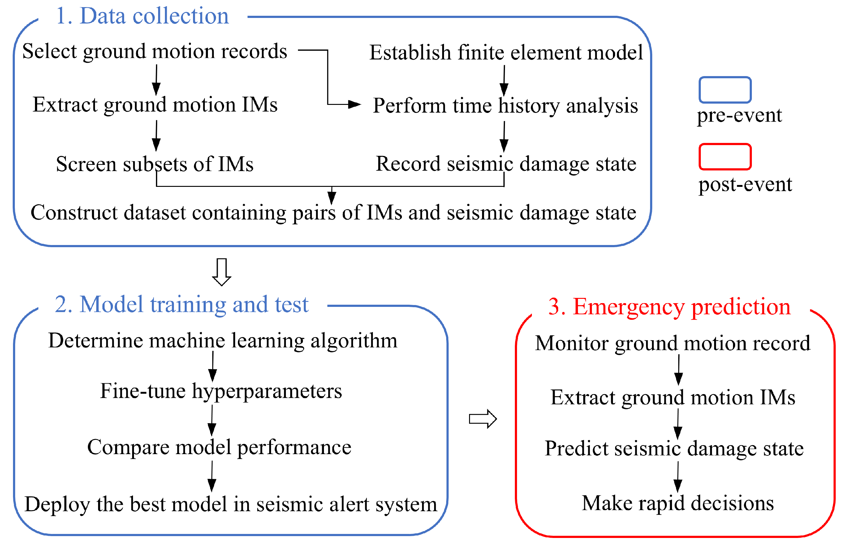
The proposed framework is shown in Figure 1, which is demonstrated in detail in the following sections with a case study.

Figure 1. Framework for rapid seismic damage state evaluation of arch dams.

4. Case Study Arch Dam

4.1. Numerical Modeling

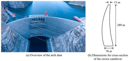
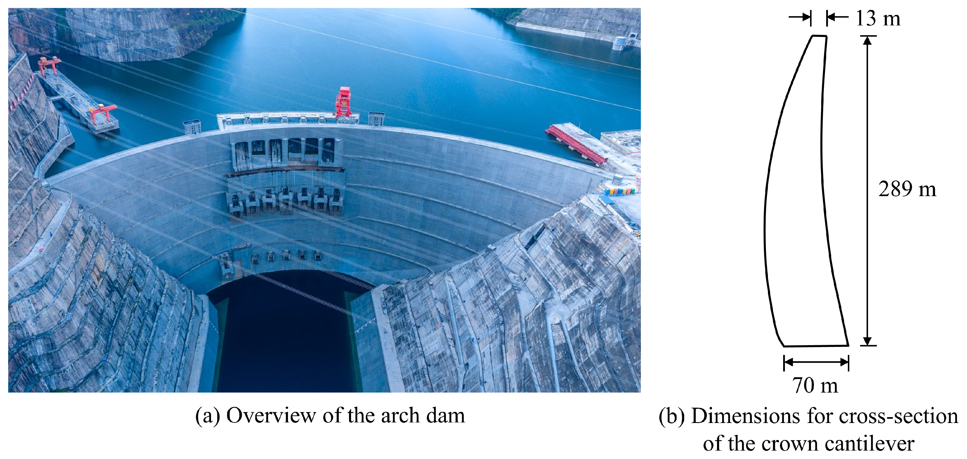
The Baihetan double-curvature arch dam situated in the strong earthquake zone of southwestern China is selected as the case study dam, as shown in Figure 2. The dam has a maximum height of 289 m and a crest arc length of 700 m. The thickness of the crown cantilever is 13 m at the crest and 70 m at the base.

Figure 2. Baihetan arch dam.

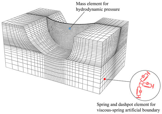
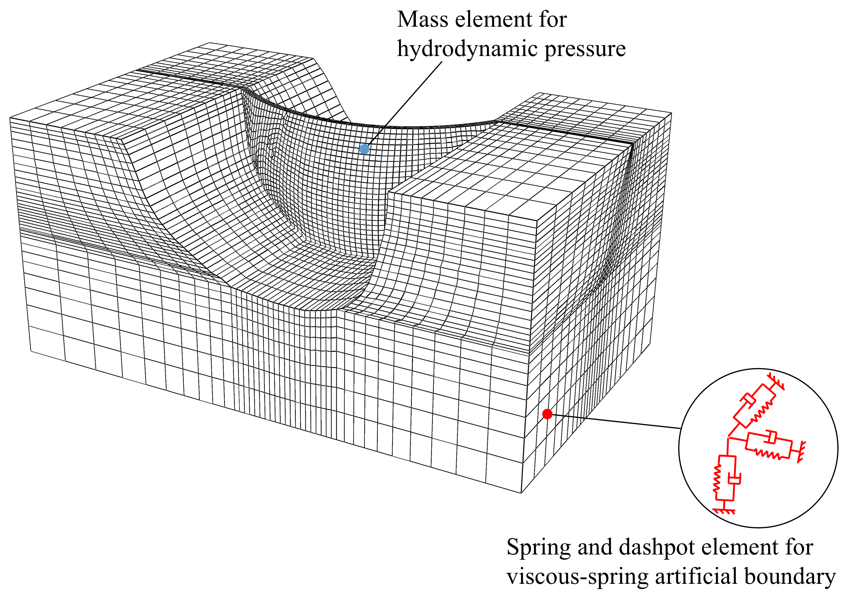
The arch dam is primarily modeled using hexahedral elements, with a limited number of pentahedral elements employed to ensure mesh continuity at the dam–foundation interface. The mesh size of the dam body is approximately 10 m in both the vertical and tangential directions and one-fourth of the arch ring thickness in the radial direction. The concrete dam consists of 4656 solid elements and 6130 nodes. The foundation domain extends to approximately 1.5 times the dam height in all five truncated directions and comprises 19,200 solid elements and 22,425 nodes. Figure 3 shows the finite element model of the Baihetan arch dam–foundation system. Recent research has recognized the radiation effects induced by a semi-infinite foundation on the earthquake response of arch dams [35,36]. To simulate the radiation damping effect, viscous-spring artificial boundaries are applied along the truncated faces [37]. The viscous-spring boundary is implemented by assigning spring and dashpot elements in both the normal and tangential directions at the nodes of the truncated boundaries, as illustrated in Figure 3. The coefficients of spring and dashpot elements are given as follows [38]:

$$K_{ln}=a_n{\displaystyle \frac{2G}{r}},K_{ls}=a_s{\displaystyle \frac{G}{2r}}$$

(10)

$$C_{ln}=b\rho c_p,C_{ls}=b\rho c_s$$

(11)

where the subscript l denotes the node number on the truncated boundary, n and s refer to the normal and tangential directions respectively, G is the shear modulus of foundation rock, r is the distance from the wave source to the node l, $\rho$ is the mass density of foundation rock, $c_p$ and $c_s$ are the velocity of P wave and S wave respectively, and $a_n$, $a_s$, and b are three coefficients, and their recommended values are provided in Reference [37].

Figure 3. Finite element discretization of the analyzed dam–foundation system.

According to the design data, the material properties adopted in this study are as follows: for dam concrete, the elastic modulus $E_c=36\mathrm{GPa}$, density ${\rho }_c=2400{\mathrm{kg}/\mathrm{m}}^3$, Poisson’s ratio ${\nu }_c=0.167$; for foundation rock, the elastic modulus $E_f=26\mathrm{GPa}$, density ${\rho }_f=2800{\mathrm{kg}/\mathrm{m}}^3$, and Poisson’s ratio ${\nu }_f=0.24$. It should be noted that the elastic modulus adopted here is a dynamic value, which is 50% higher than the static value [39,40]. A Rayleigh damping model assuming a damping ratio of 5% for the first and fifth vibration modes of the dam–foundation system is adopted. The selection of the first and fifth vibration modes aims to approximate the target damping ratio over a relatively broad frequency range while accounting for the contributions of both fundamental and higher vibration modes. Applied loads include the self-weight of the dam, hydrostatic pressure, hydrodynamic pressure, and earthquake force. The hydrodynamic pressure arising from the dam–water interaction is represented using Westergaard’s added mass approach [41]. The added mass is implemented by assigning mass elements to the nodes on the upstream face below the normal storage water level, as illustrated in Figure 3. The expression for the added mass is given as follows:

$$m_l={\displaystyle \frac{7}{8}}{A}_l{\rho }_w\sqrt{H_{0}h}$$

(12)

where $m_l$ is the added mass of node l on the upstream surface of the dam, $A_l$ is the tributary area of node l, ${\rho }_w$ is the density of water, $H_0$ is the total depth of the reservoir, and h is the water depth of node l. The seismic inputs are considered to be incident vertically and converted to equivalent forces at the truncated foundation boundaries. The equivalent forces exerted on node l can be expressed as:

$${\mathbf{F}}_l=\left({\mathbf{K}}_l{\mathbf{u}}_l^{ff}+{\mathbf{C}}_l{\dot{\mathbf{u}}}_l^{ff}+{\sigma }_l^{ff}\mathbf{n}\right)A_l$$

(13)

where ${\mathbf{u}}_l^{ff}$, ${\dot{\mathbf{u}}}_l^{ff}$, and ${\sigma }_l^{ff}$ represent the free-field displacement, velocity, and stress at node l respectively, $A_l$ is the influence area of node l, and $\mathit{n}$ is the unit outward normal vector of the truncated boundary. Detailed information on the equivalent nodal forces can be found in Reference [35].

The static solutions of the dam are taken as initial conditions in the dynamic analysis. Thus, the integral static–dynamic analysis of dams includes two steps [42]. For the initial static step, gravity loads, hydrostatic loads, and reaction forces of nodes on the truncated boundary from auxiliary static analysis are applied to obtain the static state. In the subsequent dynamic step, the equivalent nodal forces are applied to the nodes along the truncated boundary to shake the dam–foundation system. The seismic analysis of the dam–foundation system is performed using the commercial finite element software ABAQUS (version 2020).

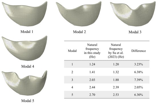
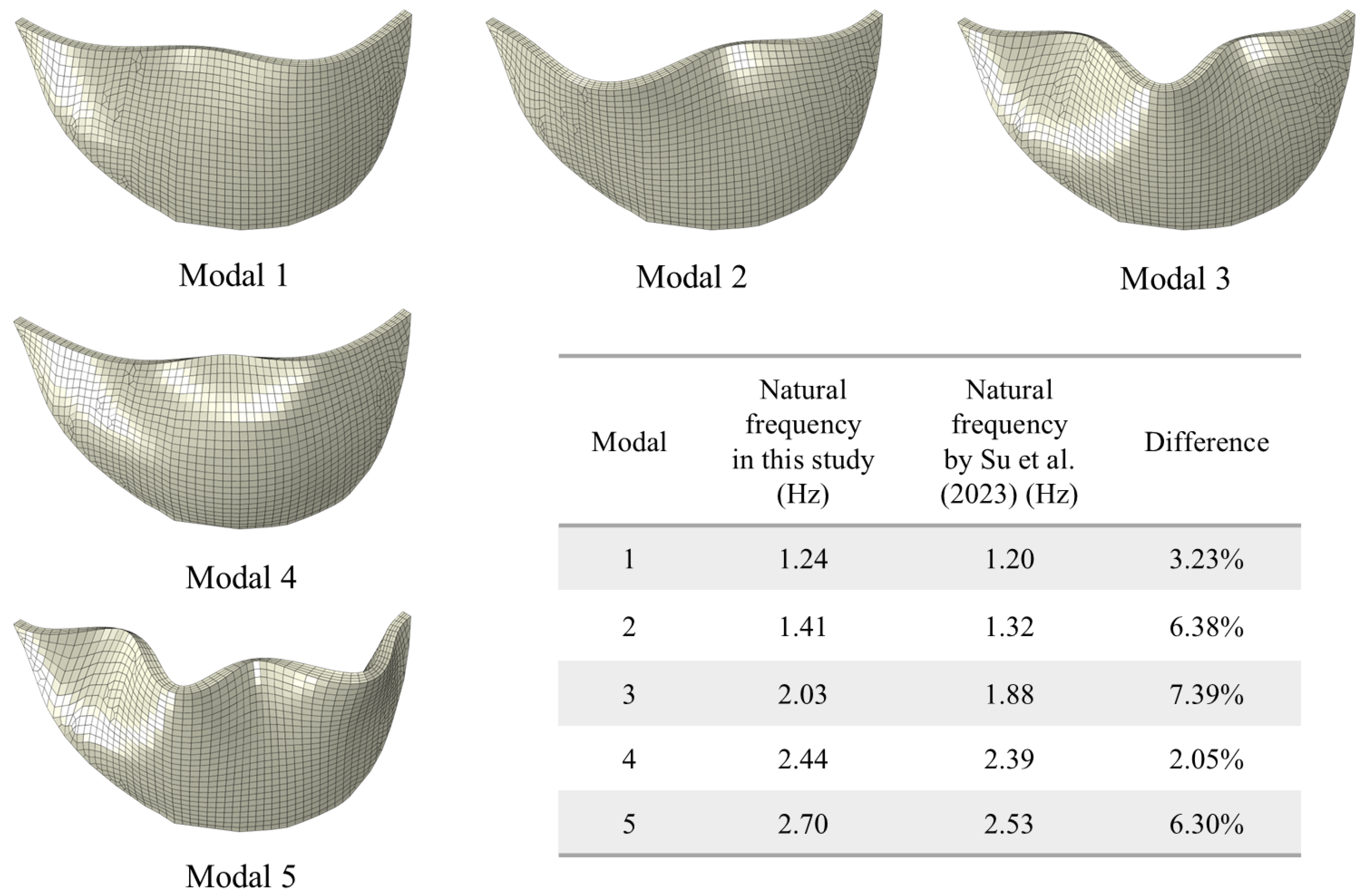
The first five modal shapes and frequencies of the arch dam are shown in Figure 4. The calculated natural frequencies show good agreement with those presented in the study [43]. The symmetric and antisymmetric bending modal shapes are consistent with those by Chen et al. [44].

Figure 4. Comparison between the first five modals of the arch dam calculated in this paper and those reported by Su et al. [43].

4.2. Damage States of Arch Dams

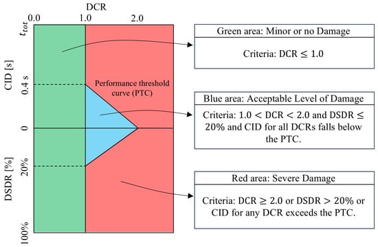
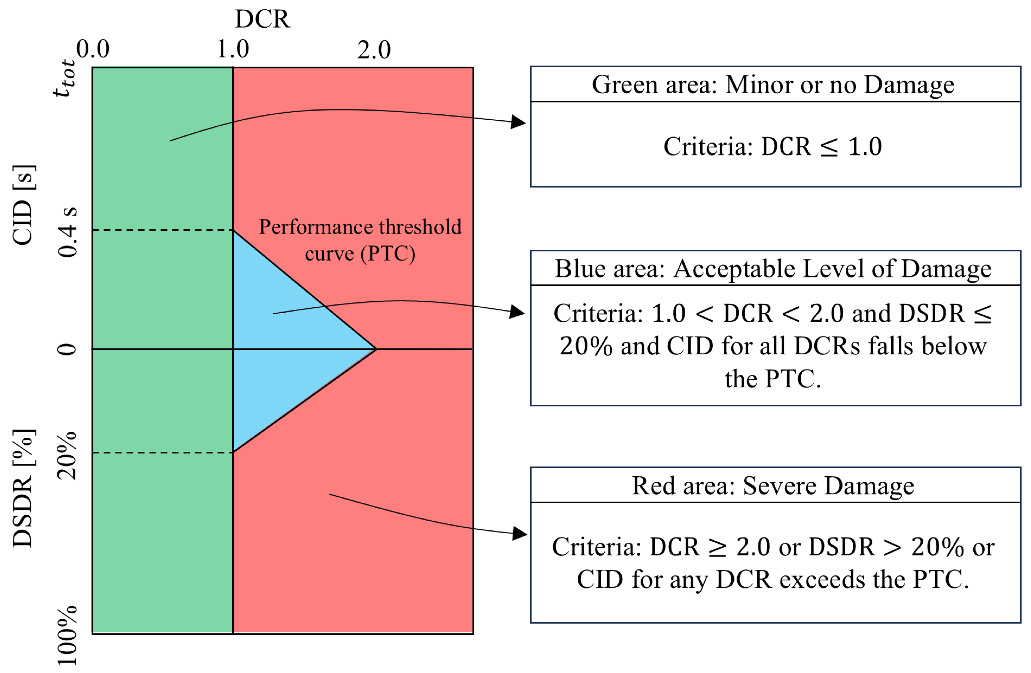
The seismic performance evaluation method for concrete dams proposed by Yusof Ghanaat [45] is adopted in this study to determine the post-earthquake damage states of arch dams. This method has been widely applied in studies on the seismic performance assessment of concrete dams [46,47,48]. The seismic performance indicators involved in this method are as follows:

• Demand capacity ratio (DCR): the ratio of the calculated maximum principal stress to the tensile strength of mass concrete.
• Cumulative inelastic duration (CID): the total time duration of stress exceeding a stress level associated with a certain DCR value.
• Damage spatial distribution ratio (DSDR): the ratio of the overstressed region to total dam cross-sectional area.

• After the seismic performance indices have been evaluated, the damage state of the arch dam can be identified as one of the following three levels:

• Minor or no Damage. When the computed stress DCRs are less than or equal to 1.0, the arch dam is considered to remain within the linear elastic range, exhibiting little or no damage.
• Acceptable Level of Damage. If the computed stress DCRs exceed 1.0, the arch dam is expected to exhibit nonlinear behavior characterized by contraction joint opening and concrete tensile cracking. The extent of joint opening and cracking is considered acceptable if the stress DCRs remain below 2.0, the overstressed region is confined to less than 20% of the upstream or downstream surface area, and the cumulative inelastic duration for all DCRs in the range of 1.0–2.0 lies below the performance curve.
• Severe Damage. If the performance criteria described above are not met, the extent of joint opening and cracking is significant and the arch dam is considered to be in a severely damaged state.

• The classification criteria of seismic damage states for arch dams are illustrated in Figure 5. The thresholds of the performance indicators are based on the mechanical interpretation of concrete tensile behavior, engineering judgment, and assumptions regarding repeated stress excursions, and are validated through case studies of Pacoima Dam and Morrow Point Dam. The stress time history of the dam surface nodes can be obtained through finite element analysis, and then the performance index values can be calculated from the stress time history. Based on the position in Figure 5, the damage state of the arch dam can be determined. Detailed information regarding the determination of these damage states can be found in Reference [45]. For simplicity, Minor or No Damage, Acceptable Level of Damage, and Severe Damage are hereafter referred to as DS0, DS1, and DS2, respectively.
  

  Figure 5. Classification of seismic damage states for arch dams; adapted from the literature [47].

4.3. Ground Motions

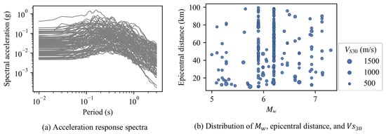
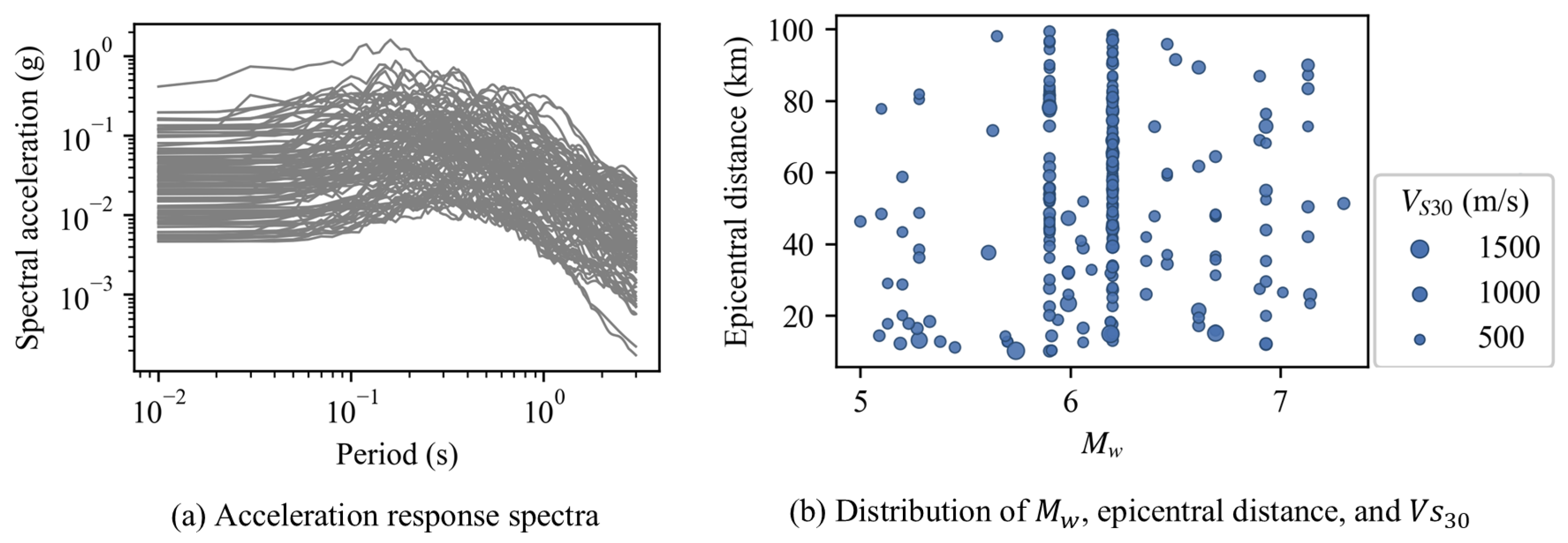
The ground motion set utilized in this study consists of 250 records selected from the NGA-West2 ground motion database developed by the Pacific Earthquake Engineering Research Center [49]. According to the engineering site conditions, the selection criteria for the ground motion records are as follows: (1) a moment magnitude between 4.5 and 7.5; (2) an epicentral distance between 10 and 100 km; and (3) a shear wave velocity greater than 500 m/s. The adopted selection procedure incorporates key seismic and site characteristics relevant to Baihetan arch dam. The acceleration response spectra and detailed information of the selected records are presented in Figure 6. Most of the selected natural ground motion records exhibit relatively low intensities, resulting in only minor structural responses. Therefore, to generate a sufficient number of samples corresponding to severe damage states, amplitude scaling is applied. The scaling of ground motion records has been widely adopted in seismic design codes and seismic damage assessment studies [39,50,51]. Previous research has indicated that amplitude scaling factors of up to 4.0 are generally acceptable [52]. The entire suite of ground motions is scaled by factors of 2.0, 3.0, and 4.0, resulting in an expanded suite of 1000 ground motions, which is employed in the present study.

Figure 6. Detailed information of the selected records.

A recorded earthquake ground motion exhibits unique characteristics, primarily because it originates from a specific fault rupture at a particular location and time and is captured at a specific site by a seismograph. These distinctive characteristics make the seismic response of arch dams highly complex and unique. Consequently, the seismic damage state of an arch dam is strongly dependent on the input ground motion. To establish the functional relationship between the input ground motion and the resulting seismic damage state using machine learning algorithms, it is essential to identify the unique characteristics of the ground motion and represent the ground motion record using one or more IMs. With reference to the IMs employed in several existing studies on the earthquake engineering of concrete dams [16,20,53,54], a total of 40 ground motion IMs are selected in this study, as listed in Table 1. These IMs exhibit substantial diversity, including: (1) acceleration-, velocity-, displacement-based, and hybrid measures; (2) frequency- and time-domain measures; and (3) cumulative and peak measures. These IMs can be computed rapidly after an earthquake, thereby ensuring the efficiency of post-earthquake damage assessment.

Table 1. Description of ground motion IMs.

No.	IMs	Symbol	Definition
1	Total duration	$t_{\mathrm{tot}}$	$t_{1.00I_A}-t_{0.00I_A}$
2	Significant duration	$t_{\mathrm{sig}}$	$t_{0.95I_A}-t_{0.05I_A}$
3	Seismological duration	$D_{5-75}$	$t_{0.75I_A}-t_{0.05I_A}$
4	Peak ground acceleration	$PGA$	$\max \left(\right|\ddot{u}\left(t\right)\left|\right)$
5	Peak ground velocity	$PGV$	$\max \left(\right|\dot{u}\left(t\right)\left|\right)$
6	Peak ground displacement	$PGD$	$\max \left(\right|u\left(t\right)\left|\right)$
7	Root-mean-square of acceleration	$a_{\mathrm{rms}}$	$\sqrt{{\displaystyle \frac{1}{t_{\mathrm{tot}}}}{\int }_0^{t_{\mathrm{tot}}}{\left(\ddot{u}\left(t\right)\right)}^{2}dt}$
8	Root-mean-square of velocity	$v_{\mathrm{rms}}$	$\sqrt{{\displaystyle \frac{1}{t_{\mathrm{tot}}}}{\int }_0^{t_{\mathrm{tot}}}{\left(\dot{u}\left(t\right)\right)}^{2}dt}$
9	Root-mean-square of displacement	$u_{\mathrm{rms}}$	$\sqrt{{\displaystyle \frac{1}{t_{\mathrm{tot}}}}{\int }_0^{t_{\mathrm{tot}}}{\left(u\left(t\right)\right)}^{2}dt}$
10	Root-square of acceleration	$a_{\mathrm{rs}}$	$\sqrt{{\int }_0^{t_{\mathrm{tot}}}{\left(\ddot{u}\left(t\right)\right)}^{2}dt}$
11	Root-square of velocity	$v_{\mathrm{rs}}$	$\sqrt{{\int }_0^{t_{\mathrm{tot}}}{\left(\dot{u}\left(t\right)\right)}^{2}dt}$
12	Root-square of displacement	$u_{\mathrm{rs}}$	$\sqrt{{\int }_0^{t_{\mathrm{tot}}}{\left(u\left(t\right)\right)}^{2}dt}$
13	Arias intensity	$I_A$	${\displaystyle \frac{\pi }{2g}}{\int }_0^{t_{\mathrm{tot}}}{\left(\ddot{u}\left(t\right)\right)}^{2}dt$
14	Specific energy density	$SED$	${\int }_0^{t_{\mathrm{tot}}}{\left(\dot{u}\left(t\right)\right)}^{2}dt$
15	Cumulative absolute velocity	$CAV$	${\int }_0^{t_{\mathrm{tot}}}\left|\ddot{u}\left(t\right)\right|dt$
16	Cumulative absolute displacement	$CAD$	${\int }_0^{t_{\mathrm{tot}}}\left|\dot{u}\left(t\right)\right|dt$
17	Cumulative absolute impulse	$CAI$	${\int }_0^{t_{\mathrm{tot}}}\left|u\left(t\right)\right|dt$
18	Shaking intensity rate	$SIR$	${I_A}_{5-75}·{\left(D_{5-75}\right)}^{-1}$
19	Acceleration spectrum intensity	$ASI$	${\int }_{0.1}^{0.5}{S}_a(T,\xi =5\%)dT$
20	Velocity spectrum intensity	$VSI$	${\int }_{0.1}^{2.5}{S}_v(T,\xi =5\%)dT$
21	Displacement spectrum intensity	$DSI$	${\int }_{2.0}^{5.0}{S}_d(T,\xi =5\%)dT$
22	Effective peak acceleration	$EPA$	${\displaystyle \frac{1}{2.5}}·{\int }_{0.1}^{0.5}{S}_a(T,\xi =5\%)dT$
23	Effective peak velocity	$EPV$	${\displaystyle \frac{1}{2.5}}·{\int }_{0.8}^{1.2}{S}_v(T,\xi =5\%)dT$
24	Effective peak displacement	$EPD$	${\displaystyle \frac{1}{2.5}}·{\int }_{2.5}^{4.0}{S}_d(T,\xi =5\%)dT$
25	First-mode spectral acceleration	$S_a\left(T_1\right)$	$S_a(T_1,\xi =5\%)$
26	First-mode spectral velocity	$S_v\left(T_1\right)$	$S_v(T_1,\xi =5\%)$
27	First-mode spectral displacement	$S_d\left(T_1\right)$	$S_d(T_1,\xi =5\%)$
28–31	Higher-mode spectral acceleration	$S_a\left(T_i\right)$	$S_a(T_i,\xi =5\%),i=2,\dots ,5$
32	Peak spectral acceleration	$PSA$	$\max \left(S_a(T,\xi =5\%)\right)$
33	Peak spectral velocity	$PSV$	$\max \left(S_V(T,\xi =5\%)\right)$
34	Peak spectral displacement	$PSD$	$\max \left(S_d(T,\xi =5\%)\right)$
35	Peak velocity to acceleration ratio	$F{R}_1$	${\displaystyle \frac{PGV}{PGA}}$
36	Peak displacement to velocity ratio	$F{R}_2$	${\displaystyle \frac{PGD}{PGV}}$
37	Peak square velocity to acceleration ratio	$F{R}_3$	${\displaystyle \frac{PG{V}^2}{PGA}}$
38	Riddell acceleration intensity	$R{I}_a$	$PGA·{t_{\mathrm{sig}}}^{1/3}$
39	Riddell velocity intensity	$R{I}_v$	$PG{V}^{2/3}·{t_{\mathrm{sig}}}^{1/3}$
40	Riddell displacement intensity	$R{I}_d$	$PGD·{t_{\mathrm{sig}}}^{1/3}$

Note: $\ddot{u}\left(t\right)$, $\dot{u}\left(t\right)$, and u(t) are acceleration, velocity, and displacement time histories respectively; g is gravitational acceleration.

5. Application of the Proposed Framework to the Selected Arch Dam

5.1. Dataset Generation

As described in Section 4.3, 1000 ground motion records are utilized to conduct the earthquake time-history analyses of the arch dam. The seismic damage state of the arch dam is determined using the Ghanaat’s method based on its stress response. The ground motion records employed in this study are three-component records, namely the cross-stream (H₁), stream (H₂), and vertical (V) components, and each component is characterized by the 40 IMs in Table 1. Thus, each record is characterized by 120 IMs. The 120 intensity measures associated with one record (feature of a sample), together with the corresponding seismic damage state of the arch dam (label of a sample), form a single sample; the resulting dataset comprises 1000 such samples in total. The number of samples in each seismic damage state is presented in Table 2.

Table 2. The number of samples for each seismic damage state.

Damage state	DS0	DS1	DS2
Number of samples	704	97	199

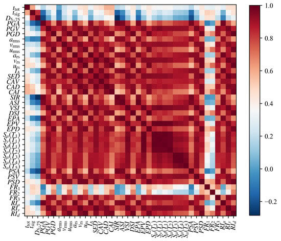
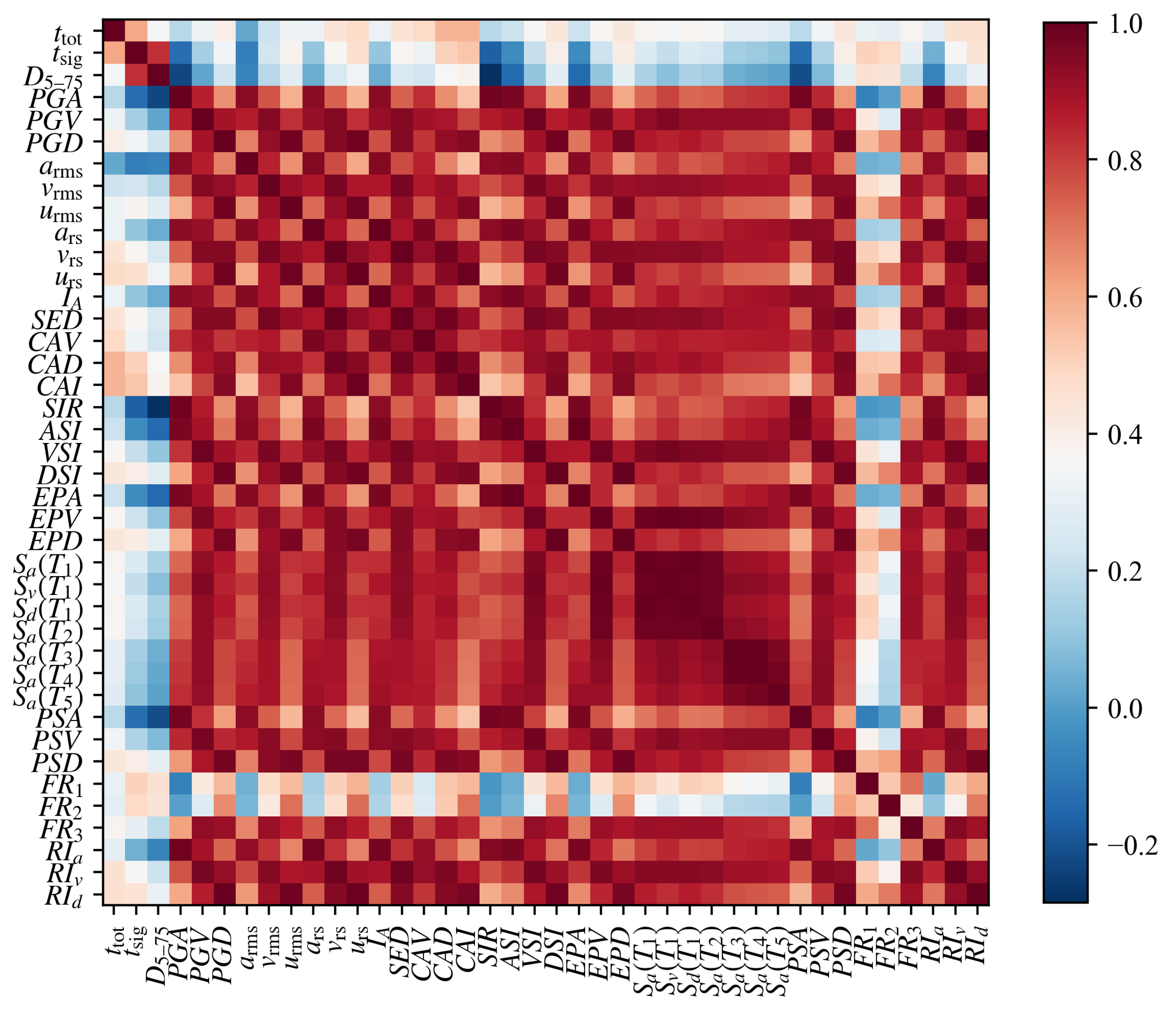
Due to the amplitude scaling of ground motions and the similarities in the definition of IMs, correlations may exist among the 120 IMs. To quantitatively evaluate the correlations, the Spearman correlation coefficient is introduced to investigate correlations between two variables. It varies between −1 and +1 with 0 implying no correlation. Generally, when the absolute value of the correlation coefficient is greater than 0.8, the two variables can be regarded as strongly correlated. Figure 7 illustrates the correlations among the 40 IMs of H₂ component. Dark red corresponds to strong positive correlations, and blue corresponds to low positive or negative correlations. It is evident that some IMs are highly correlated, such as between $PGA$ and $a_{\mathrm{rms}}$, $I_A$ and $a_{\mathrm{rs}}$, and $EPA$ and $ASI$. IMs with strong correlations contain overlapping and redundant seismic information and may reduce accuracy and efficiency of the prediction machine learning models. Therefore, to obtain models with improved predictive capability, it is necessary to perform screening of input IMs (commonly referred to as feature selection in the field of machine learning).

Figure 7. Correlation map among the 40 IMs of H₂ component.

Recursive feature elimination (RFE) is used in this study to select the informative IMs. This method consists of two steps. First, a classifier capable of assigning weights to the features is trained using the full feature set, and the importance of each feature is derived. Subsequently, the least important features are removed from the current feature set. This process is recursively repeated on the reduced set until the target number of selected features is reached. The RFE algorithm is conveniently implemented using the application programming interface provided by the scikit-learn machine learning library [55]. Scikit-learn is an open-source Python library that provides efficient implementations of a wide range of machine learning algorithms and related tools for model development and evaluation [56].

Five feature scenarios are considered in this study, with the number of features being 1, 5, 10, 20, and 120, respectively. The outcome of feature selection by RFE is shown in Table 3. It is noted that the selected intensity measures are mainly derived from the H₁ and H₂ components rather than from the V component, indicating that the H₁ and H₂ components have a greater influence on the seismic damage state of the arch dam compared with the V component. This observation is consistent with common engineering experience. It is also noted that spectral-type IMs dominate the selected feature subset. In addition, the only IM selected in the 1-feature scenario is the $S_v\left(T_1\right)$ of H₂ component, indicating that the $S_v\left(T_1\right)$ of H₂ component is the IM most strongly correlated with the seismic damage of arch dams.

Table 3. Feature selection results for the five feature scenarios.

Feature Scenarios	Features Selected
1-feature	H2: $S_v\left(T_1\right)$
5-feature	H1: $S_a\left(T_5\right)$, $PSV$; H2: $EPD$, $S_a\left(T_1\right)$, $S_v\left(T_1\right)$
10-feature	H1: $SED$, $S_a\left(T_2\right)$, $S_a\left(T_5\right)$, $PSV$; H2: $EPD$, $S_a\left(T_1\right)$, $S_v\left(T_1\right)$, $S_a\left(T_5\right)$, $PSV$; V: $PSV$
20-feature	H1: $PGD$, $SED$, $ASI$, $S_a\left(T_2\right)$, $S_a\left(T_5\right)$, $PSV$; H2: $SED$, $DSI$, $EPV$, $EPD$, $S_a\left(T_1\right)$, $S_v\left(T_1\right)$, $S_d\left(T_1\right)$, $S_a\left(T_3\right)$, $S_a\left(T_4\right)$, $S_a\left(T_5\right)$, $PSV$, $R{I}_v$; V: $S_a\left(T_3\right)$, $PSV$
120-feature	All features

5.2. Training and Test of Machine Learning Models

As described in Section 2, six classical machine learning algorithms, including Logistic Regression (LR), Decision Tree (DT), K-Nearest Neighbors (KNN), Support Vector Machine (SVM), Artificial Neural Networks (ANN), and Random Forest (RF), are adopted to establish the mapping between the ground motion IMs and the seismic damage state of the arch dam. These six algorithms have been demonstrated to be reliable in the fast damage assessment task for other types of structures [8,9]. In addition to the choice of machine learning algorithm, the hyperparameter settings of each algorithm also affect the performance of the prediction model. Therefore, to obtain a prediction model with higher accuracy, grid search combined with 5-fold cross validation is employed in this study to tune the hyperparameters. Grid search systematically evaluates all predefined combinations of hyperparameter values by training and validating the model under each combination. Although grid search can be computationally expensive, it provides a straightforward and exhaustive strategy for identifying suitable hyperparameter settings within a predefined search space. In the 5-fold cross validation, the training dataset is randomly partitioned into 5 equal-sized subsets. For each hyperparameter combination, 4 subsets are used as training data, and the remaining subset is adopted as validation data. This process is repeated until each of the 5 parts is used exactly once as the validation set. The final evaluation score is obtained by averaging the scores from the 5 validation runs. The major hyperparameters considered for each algorithm, along with their corresponding search ranges, are summarized in Table 4.

Table 4. The tuned hyperparameters for the six machine learning algorithms.

Algorithms	Hyperparameters Tuned	Values Considered
LR	penalty	l1, l2, elasticnet, None
	C	1, 10, 100
DT	max_depth	3, 5, 7, 9, 11
	max_features	sqrt, log2, None
KNN	n_neighbors	5, 10, 15
	p	1, 2
SVM	kernel	linear, rbf, poly
	C	1, 10, 100
	gamma	scale, auto
ANN	hidden_layer_sizes	(5,), (10,), (5, 5), (10, 10)
	activation	identity, logistic, tanh, relu
	learning_rate_init	0.01, 0.001
RF	n_estimators	50, 100, 150
	max_depth	3, 4, 5
	max_samples	0.8, 0.9, 1.0

Note: the hyperparameters and their values are not described in detail herein; comprehensive information can be found in the scikit-learn library documentation [57].

The dataset established in Section 5.1 is randomly divided into the training subset (70%, 700 samples) and the test subset (30%, 300 samples). The data are split in a stratified manner to ensure that the class proportions in the training and test datasets remain consistent. Hyperparameter optimization and model training under different feature scenarios are performed exclusively using the training dataset, and the test dataset is used solely to evaluate and compare the predictive performance of the trained candidate models. To eliminate the influence of feature distributions and measurement units, min-max scaling is applied to each feature such that all feature values fall within the range [0, 1]. It should be emphasized that the dataset exhibits class imbalance. The number of DS0 samples is substantially greater than that of the other two classes, as shown in Table 2. To mitigate the effect of this imbalance, class weights are incorporated into the machine learning algorithms. The training and test of the six machine learning algorithms employed in this study are conducted using the scikit-learn machine learning library (version 1.7.2). A random seed of 42 was adopted to improve the reproducibility of the data partitioning and model training. Hyperparameter optimization was performed using grid search combined with five-fold cross-validation. Except for the hyperparameters included in the grid search, all remaining parameters were set to their default values in scikit-learn. The final optimized hyperparameters of the machine learning models are summarized in Table 5.

Table 5. Optimized hyperparameters of the machine learning models.

Feature Scenarios	Models	Optimized Hyperparameters
1-feature	LR	‘C’: 1, ‘penalty’: ‘l2’
	DT	‘max_depth’: 3, ‘max_features’: ‘sqrt’
	KNN	‘n_neighbors’: 15, ‘p’: 1
	SVM	‘C’: 1, ‘gamma’: ‘scale’, ‘kernel’: ‘linear’
	ANN	‘activation’: ‘logistic’, ‘hidden_layer_sizes’: (5, 5), ‘learning_rate_init’: 0.01
	RF	‘max_depth’: 4, ‘max_samples’: 0.8, ‘n_estimators’: 50
5-feature	LR	‘C’: 1, ‘penalty’: ‘l2’
	DT	‘max_depth’: 7, ‘max_features’: ‘sqrt’
	KNN	‘n_neighbors’: 10, ‘p’: 1
	SVM	‘C’: 1, ‘gamma’: ‘scale’, ‘kernel’: ‘poly’
	ANN	‘activation’: ‘tanh’, ‘hidden_layer_sizes’: (5,), ‘learning_rate_init’: 0.01
	RF	‘max_depth’: 5, ‘max_samples’: 0.8, ‘n_estimators’: 100
10-feature	LR	‘C’: 1, ‘penalty’: ‘elasticnet’
	DT	‘max_depth’: 11, ‘max_features’: None
	KNN	‘n_neighbors’: 10, ‘p’: 2
	SVM	‘C’: 100, ‘gamma’: ‘scale’, ‘kernel’: ‘poly’
	ANN	‘activation’: ‘tanh’, ‘hidden_layer_sizes’: (10, 10), ‘learning_rate_init’: 0.01
	RF	‘max_depth’: 5, ‘max_samples’: 0.9, ‘n_estimators’: 150
20-feature	LR	‘C’: 10, ‘penalty’: ‘l1’
	DT	‘max_depth’: 11, ‘max_features’: None
	KNN	‘n_neighbors’: 10, ‘p’: 1
	SVM	‘C’: 100, ‘gamma’: ‘scale’, ‘kernel’: ‘poly’
	ANN	‘activation’: ‘tanh’, ‘hidden_layer_sizes’: (10,), ‘learning_rate_init’: 0.01
	RF	‘max_depth’: 5, ‘max_samples’: 0.9, ‘n_estimators’: 100
120-feature	LR	‘C’: 100, ‘penalty’: ‘l2’
	DT	‘max_depth’: 9, ‘max_features’: None
	KNN	‘n_neighbors’: 5, ‘p’: 2
	SVM	‘C’: 100, ‘gamma’: ‘scale’, ‘kernel’: ‘rbf’
	ANN	‘activation’: ‘tanh’, ‘hidden_layer_sizes’: (10,), ‘learning_rate_init’: 0.01
	RF	‘max_depth’: 5, ‘max_samples’: 0.9, ‘n_estimators’: 100

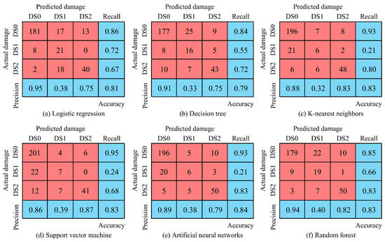
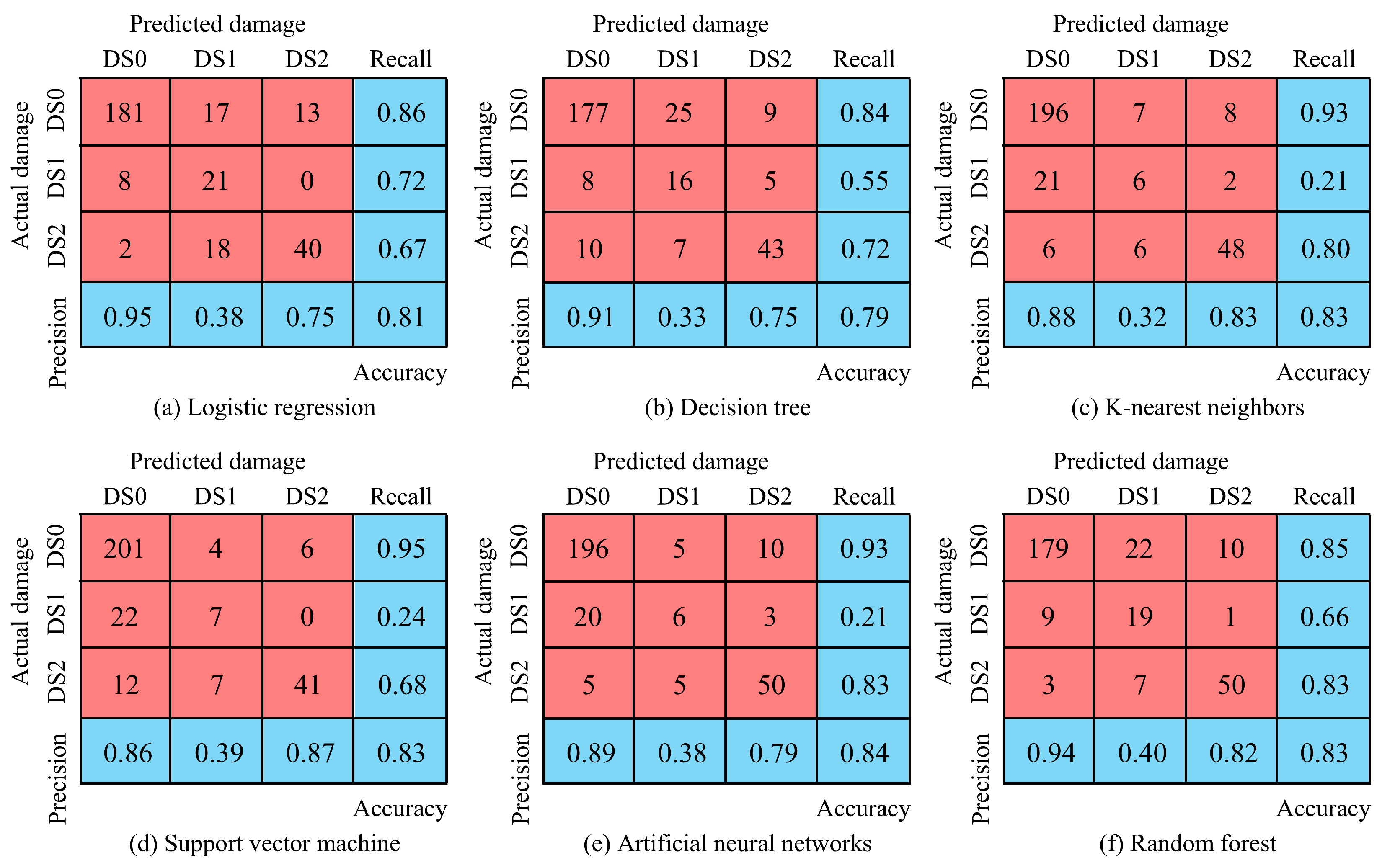
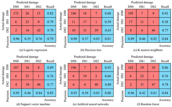
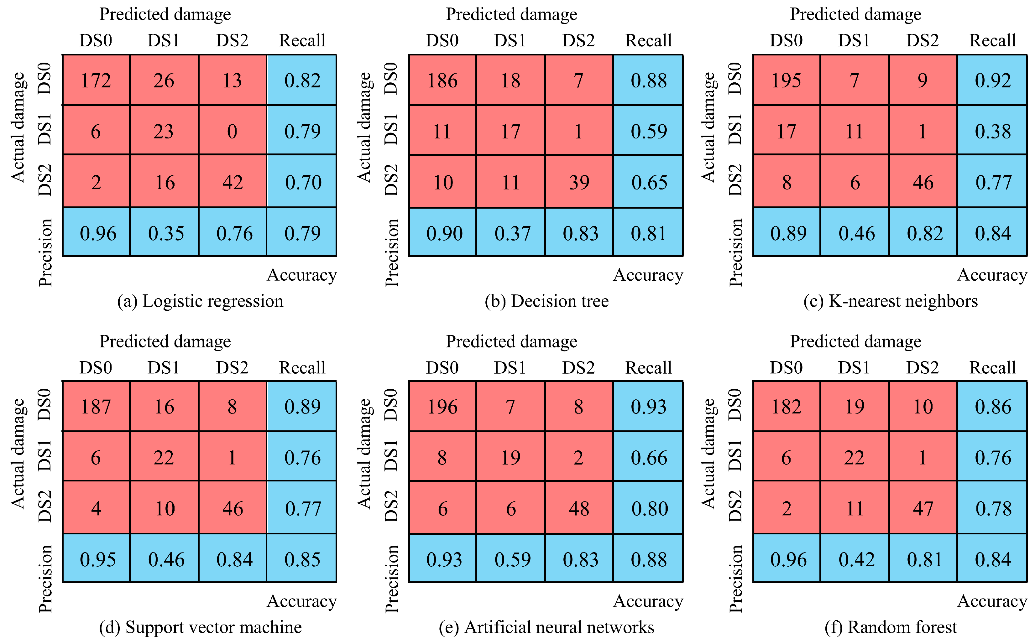
The test results on the test dataset can be illustrated using a confusion matrix. In this matrix, the diagonal elements correspond to samples that are correctly classified by the machine learning model, whereas the off-diagonal elements denote misclassified samples. The performance of the machine learning models can be evaluated in terms of precision, recall, and accuracy. Precision is defined as the proportion of predicted labels that are correctly assigned, while recall denotes the proportion of actual labels that are correctly identified. Accuracy is calculated as the ratio of correctly predicted samples to the total number of samples. High values of precision, recall, and accuracy indicate strong predictive performance of the machine learning models. The confusion matrices and the corresponding precision, recall, and accuracy values for the trained machine learning models are presented in the next section.

5.3. Results and Discussion

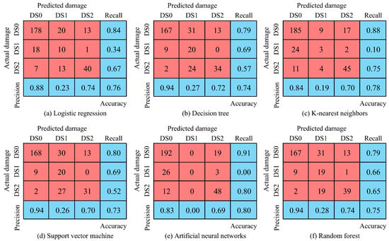
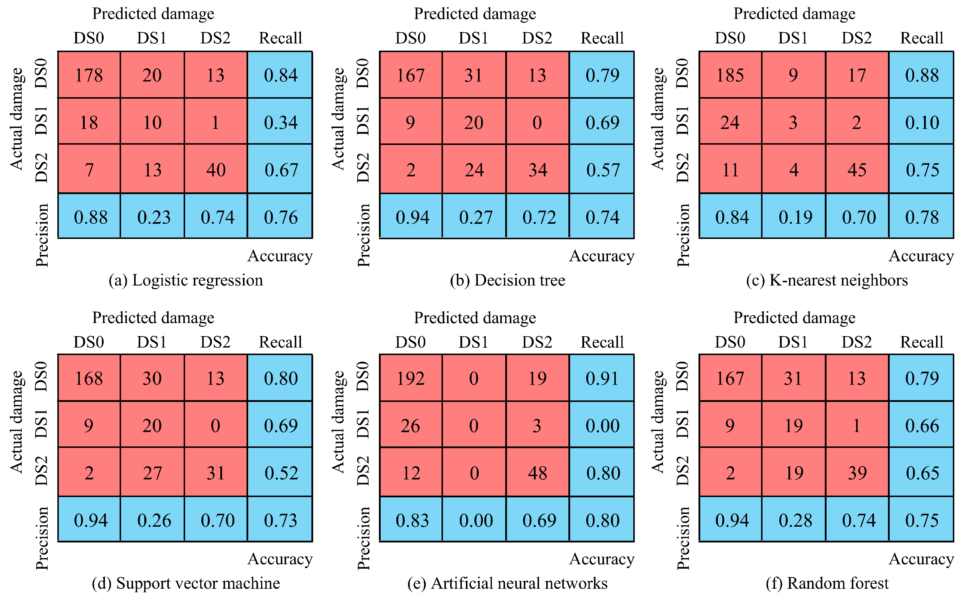
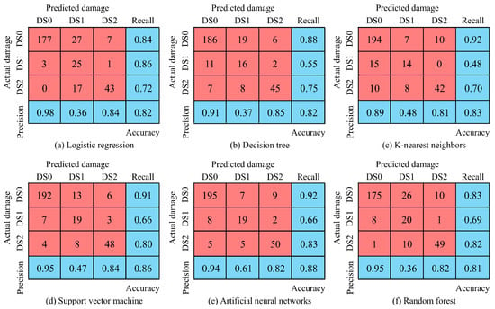
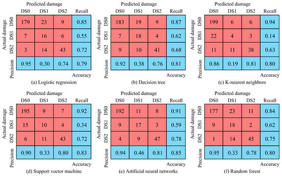
After the 30 machine learning models corresponding to the six machine learning algorithms and the five feature scenarios are trained, their predictive performance is evaluated on the test dataset. The test results for the five feature scenarios are presented in Figure 8, Figure 9, Figure 10, Figure 11 and Figure 12, respectively. In these figures, the red panels show the confusion matrices, whereas the blue panels present the precision, recall, and accuracy metrics. The following observations can be drawn from these figures:

Figure 8. Test results of the six machine learning models for the 1-feature scenario.

Figure 9. Test results of the six machine learning models for the 5-feature scenario.

Figure 10. Test results of the six machine learning models for the 10-feature scenario.

Figure 11. Test results of the six machine learning models for the 20-feature scenario.

Figure 12. Test results of the six machine learning models for the 120-feature scenario.

• For each of the 30 machine learning models, the precision and recall values for DS1 are relatively lower than those for the other two damage states, DS0 and DS2. This can be attributed to the fact that the number of DS1 samples in the dataset is comparatively small. Consequently, the machine learning models have fewer opportunities to learn the characteristic patterns associated with DS1, making them more susceptible to confusion with the neighboring damage states.
• Considering the overall performance in terms of accuracy, precision, and recall, the ANN model under the 20-feature scenario is identified as the optimal model. It achieves an total accuracy of 0.88, with precision values of 0.94, 0.61, and 0.82 and recall values of 0.92, 0.66, and 0.83 for DS0, DS1, and DS2, respectively. Owing to its satisfactory predictive performance, this trained model can be integrated into earthquake alerting systems to facilitate rapid post-earthquake assessment of arch dam damage states.
• For post-earthquake emergency management, the misclassification of DS2 deserves particular attention, as underestimating the actual damage state may delay necessary emergency responses. The confusion matrix of the ANN model under the 20-feature scenario reveals that, among the 60 actual DS2 samples, 50 are correctly classified, while 5 are misclassified as DS1 and the remaining 5 as DS0. Accordingly, the recall for DS2 reaches 0.83, indicating that the model has a relatively high accuracy in identifying severe damage states.

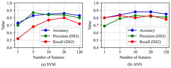
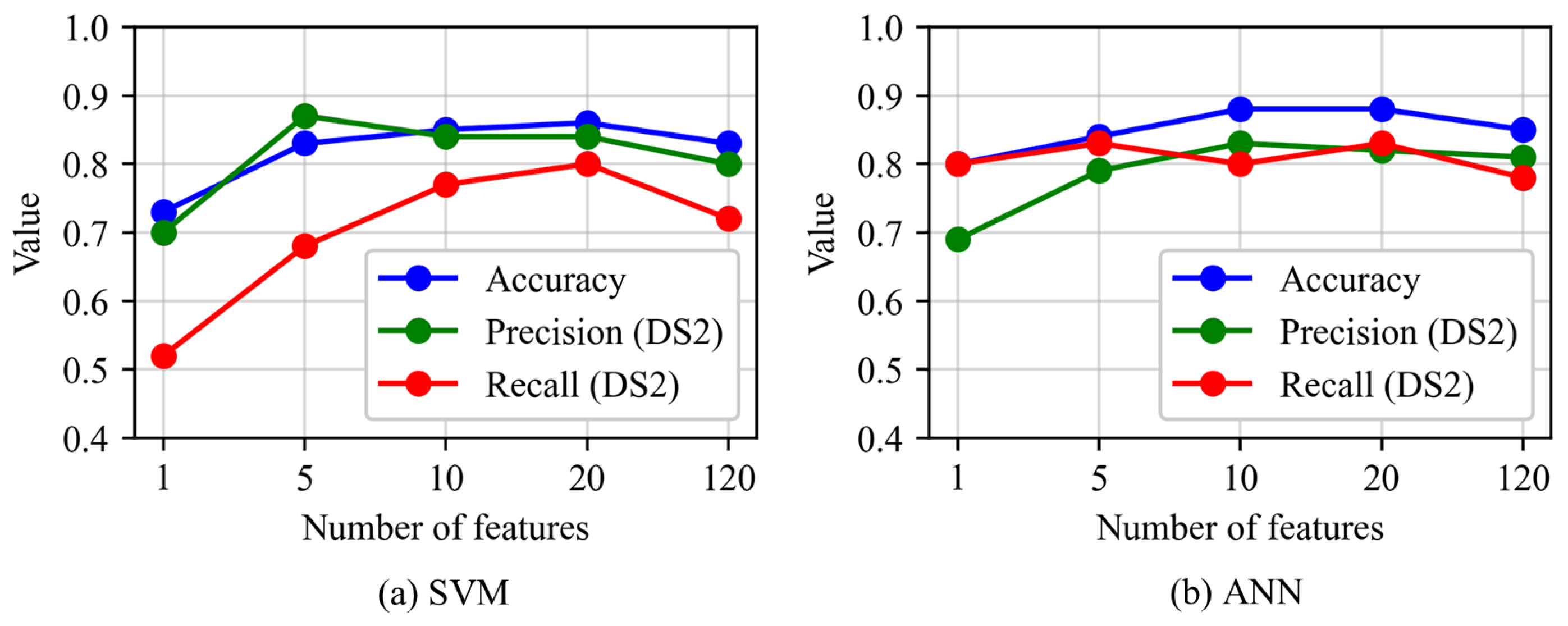
Figure 13 illustrates the variations in overall accuracy, precision for DS2, and recall for DS2 with the number of selected features for the SVM and ANN models. These two models were selected as representatives because, as can be seen from the confusion matrices, they generally exhibit better predictive performance than the other algorithms. The machine learning models developed under the 1-feature scenario consistently exhibit poorer predictive performance than those developed under the other feature scenarios. This finding indicates that a single IM cannot adequately represent the characteristics of ground motions related to arch dam damage. Therefore, multiple complementary features are required to provide sufficient information for reliable damage state prediction. Although some of the 120 IMs are highly correlated, the machine learning models under the 120-feature scenario do not exhibit a noticeable deterioration in predictive performance compared with those under the 5-, 10-, and 20-feature scenarios. This finding suggests that the machine learning algorithms considered in this study are capable of effectively handling highly correlated features and are not overly sensitive to feature redundancy.

Figure 13. Variations in accuracy, precision for DS2, and recall for DS2 with the number of features.

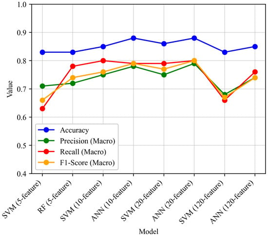
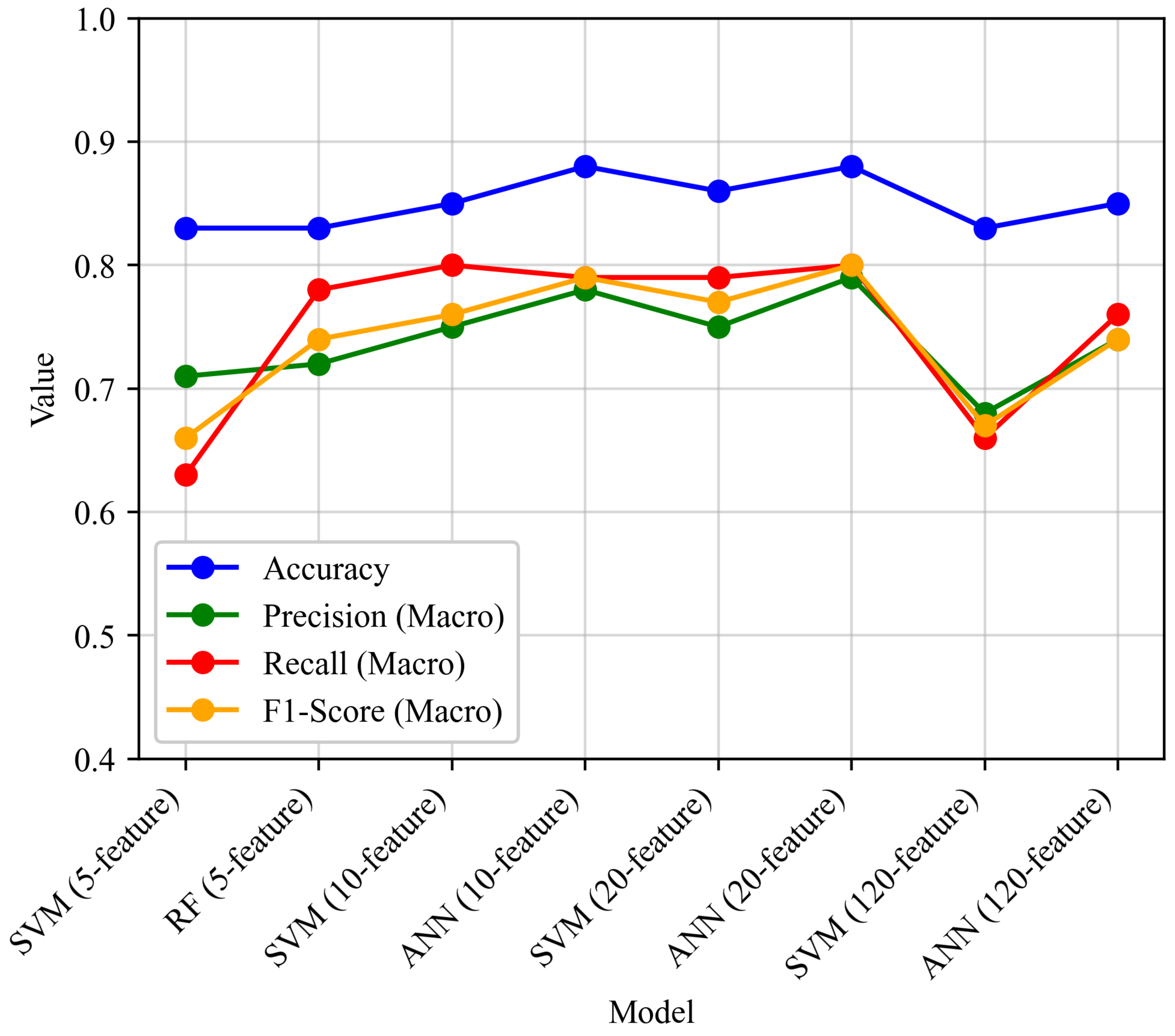
To further evaluate the classification performance of the developed models, eight models preliminarily selected by accuracy are chosen for additional comparison using macro-averaged precision, recall, and F1-score, as shown in Figure 14. Unlike overall accuracy, macro-averaged metrics assign equal importance to each damage state, thereby providing a more balanced assessment of classification performance in the presence of class imbalance. As illustrated in Figure 14, the ANN model under the 20-feature scenario achieves the best overall performance among the eight models, with an accuracy of 0.88 and macro-averaged precision, recall, and F1-score of 0.79, 0.80, and 0.80, respectively. These findings further support the selection of the ANN model under the 20-feature scenario as the best-performing model.

Figure 14. Comparison of accuracy and macro-averaged metrics for the eight models.

Table 6 summarizes a set of well-performing models selected from Figure 8, Figure 9, Figure 10, Figure 11 and Figure 12. Total accuracy is adopted as one of the selection criteria. In addition, because the prediction of DS2 is more critical for the emergency management of arch dams than that of the other two damage states, the precision for DS2 is also adopted as a selection criterion. It is observed that the SVM and ANN algorithms outperform the other four algorithms in assessing the seismic damage states of arch dams. Both the total accuracy and the precision for DS2 of the selected models exceed 0.8, indicating that they are reliable for assessing the seismic damage states of arch dams. In addition to deploying only the optimal model, this set of well-performing models can also be deployed simultaneously in earthquake alert systems. The final damage state of the arch dam can then be determined using a majority voting scheme, in which each model casts one vote for its predicted damage state, and the damage state receiving the largest number of votes is adopted as the final prediction.

Table 6. Selected set of well-performing models.

Feature Scenarios	Models Selected
1-feature	None (neither the total accuracy nor the precision for DS2 exceeds 0.8).
5-feature	SVM (0.83, 0.87)
10-feature	SVM (0.85, 0.84), ANN (0.88, 0.83)
20-feature	SVM (0.86, 0.84), ANN (0.88, 0.82)
120-feature	ANN (0.85, 0.81)

Note: the two values in parentheses correspond to the total accuracy and the precision for DS2, respectively.

6. Conclusions

Rapid and reliable assessment of earthquake-induced damage in arch dams is essential for effective dam emergency management. In this study, a rapid seismic damage assessment method for arch dams based on machine learning algorithms is proposed and verified through a case study of the Baihetan arch dam in southwestern China. The following conclusions can be drawn from this study:

(1)

In feature selection, the selected IMs are mainly from the H₁ and H₂ components, indicating that the horizontal components play a more important role than the V component in characterizing the seismic damage of arch dams. $S_v\left(T_1\right)$ of H₂ component exhibits the strongest correlation with the seismic damage of arch dams.

(2)

The six models developed under the 1-feature scenario consistently exhibit poorer predictive performance, indicating that considering only the single most important IM is insufficient for developing prediction models and that multiple IMs should be considered.

(3)

Under the 5-, 10-, 20-, and 120-feature scenarios, the SVM and ANN algorithms outperform the other four algorithms in terms of both the total accuracy and the precision for DS2. Therefore, these two algorithms are recommended for developing prediction models for seismic damage of arch dams.

(4)

Among all the developed prediction models, the ANN model under the 20-feature scenario achieves the best overall predictive performance. It attains a total accuracy of 0.88. The precision values for DS0, DS1, and DS2 are 0.94, 0.61, and 0.82, respectively, while the corresponding recall values are 0.92, 0.66, and 0.83. This model can be deployed in earthquake alerting systems to rapidly evaluate the seismic damage state of arch dams using ground motion data monitored during earthquakes, thereby facilitating dam emergency decision-making.

Despite its promising predictive performance, the proposed framework has certain limitations. First, the developed prediction models can assess the overall seismic damage state of an arch dam but cannot identify the specific locations of damage within the dam structure. Future research will focus on incorporating damage location information into the dataset to enable more detailed damage assessment. Second, the developed prediction models have been validated only through a case study of the Baihetan arch dam. Their generalizability to other arch dams with different structural characteristics and site conditions requires further investigation. Classical machine learning algorithms (using ground motion IMs as input features) are employed in this study to develop the prediction models for the seismic damage state of arch dams. The use of deep learning algorithms may further enhance the predictive performance of the models. Thus, another extension of this work can be directed towards convolutional neural networks (using time-frequency representations of ground motions as input features) and recurrent neural networks (using ground motion time histories as input features).

References

- Wang, J.T.; Zhang, M.X.; Jin, A.Y.; Zhang, C.H. Seismic fragility of arch dams based on damage analysis. Soil Dyn. Earthq. Eng. 2018, 109, 58–68. [Google Scholar] [CrossRef] [Scilit]
- Liang, H.; Tu, J.; Guo, S.; Liao, J.; Li, D.; Peng, S. Seismic fragility analysis of a High Arch Dam-Foundation System based on seismic instability failure mode. Soil Dyn. Earthq. Eng. 2020, 130, 105981. [Google Scholar] [CrossRef] [Scilit]
- Wang, Y.; Zheng, Z.; Ji, D.; Pan, X.; Tian, A. Machine learning-driven probabilistic seismic demand model with multiple intensity measures and applicability in seismic fragility analysis for nuclear power plants. Soil Dyn. Earthq. Eng. 2023, 171, 107966. [Google Scholar] [CrossRef] [Scilit]
- Xie, Y.; Sichani, M.E.; Padgett, J.E.; DesRoches, R. The promise of implementing machine learning in earthquake engineering: A state-of-the-art review. Earthq. Spectra 2020, 36, 1769–1801. [Google Scholar] [CrossRef] [Scilit]
- Xie, Y. Deep Learning in Earthquake Engineering: A Comprehensive Review. ASCE OPEN: Multidiscip. J. Civ. Eng. 2025, 3, 03125001. [Google Scholar] [CrossRef] [Scilit]
- Thai, H.T. Machine learning for structural engineering: A state-of-the-art review. Structures 2022, 38, 448–491. [Google Scholar] [CrossRef] [Scilit]
- Amini Pishro, A. Machine learning applications in reinforced concrete structures: A comprehensive review of methods, challenges, and future directions. Structures 2026, 89, 112103. [Google Scholar] [CrossRef] [Scilit]
- Xu, Y.; Lu, X.; Tian, Y.; Huang, Y. Real-Time Seismic Damage Prediction and Comparison of Various Ground Motion Intensity Measures Based on Machine Learning. J. Earthq. Eng. 2022, 26, 4259–4279. [Google Scholar] [CrossRef] [Scilit]
- Mangalathu, S.; Hwang, S.H.; Choi, E.; Jeon, J.S. Rapid seismic damage evaluation of bridge portfolios using machine learning techniques. Eng. Struct. 2019, 201, 109785. [Google Scholar] [CrossRef] [Scilit]
- Kourehpaz, P.; Molina Hutt, C. Machine Learning for Enhanced Regional Seismic Risk Assessments. J. Struct. Eng. 2022, 148, 04022126. [Google Scholar] [CrossRef] [Scilit]
- Morfidis, K.; Kostinakis, K. Approaches to the rapid seismic damage prediction of r/c buildings using artificial neural networks. Eng. Struct. 2018, 165, 120–141. [Google Scholar] [CrossRef] [Scilit]
- Ozturk, B.; Hussein, A.F.; El Naggar, M.H. Machine Learning-Based Seismic Damage Assessment of a Bridge Portfolio in Cohesive Soil. Buildings 2025, 15, 1682. [Google Scholar] [CrossRef] [Scilit]
- Bhatta, S.; Dang, J. Seismic damage prediction of RC buildings using machine learning. Earthq. Eng. Struct. Dyn. 2023, 52, 3504–3527. [Google Scholar] [CrossRef] [Scilit]
- Zheng, X.; Wei, B.; Jiang, L.; Lai, Z.; Chen, J.; Chen, M.; Xiao, B.; Zhang, R.; Yang, Z. Active learning-based regional seismic risk assessment of high-speed railway bridges. Adv. Eng. Inform. 2025, 66, 103470. [Google Scholar] [CrossRef] [Scilit]
- Xu, J.G.; Feng, D.C.; Mangalathu, S.; Jeon, J.S. Data-driven rapid damage evaluation for life-cycle seismic assessment of regional reinforced concrete bridges. Earthq. Eng. Struct. Dyn. 2022, 51, 2730–2751. [Google Scholar] [CrossRef] [Scilit]
- Hariri-Ardebili, M.A.; Barak, S. A series of forecasting models for seismic evaluation of dams based on ground motion meta-features. Eng. Struct. 2020, 203, 109657. [Google Scholar] [CrossRef] [Scilit]
- Hariri-Ardebili, M.A.; Chen, S.; Mahdavi, G. Machine learning-aided PSDM for dams with stochastic ground motions. Adv. Eng. Inform. 2022, 52, 101615. [Google Scholar] [CrossRef] [Scilit]
- Segura, R.; Padgett, J.E.; Paultre, P. Metamodel-Based Seismic Fragility Analysis of Concrete Gravity Dams. J. Struct. Eng. 2020, 146, 04020121. [Google Scholar] [CrossRef] [Scilit]
- Segura, R.; Padgett, J.; Paultre, P. Expected seismic performance of gravity dams using machine learning techniques. Bull. N. Zealand Soc. Earthq. Eng. 2021, 54, 58–68. [Google Scholar] [CrossRef] [Scilit]
- Li, Z.; Wu, Z.; Lu, X.; Zhou, J.; Chen, J.; Liu, L.; Pei, L. Efficient seismic risk analysis of gravity dams via screening of intensity measures and simulated non-parametric fragility curves. Soil Dyn. Earthq. Eng. 2022, 152, 107040. [Google Scholar] [CrossRef] [Scilit]
- Hastie, T.; Friedman, J.; Tibshirani, R. The Elements of Statistical Learning; Springer Series in Statistics; Springer: New York, NY, USA, 2001. [Google Scholar] [CrossRef] [Scilit]
- Vapnik, V.N. The Nature of Statistical Learning Theory; Springer: New York, NY, USA, 2000. [Google Scholar] [CrossRef] [Scilit]
- Hosmer, D.W., Jr.; Lemeshow, S.; Sturdivant, R.X. Applied Logistic Regression; John Wiley & Sons: Hoboken, NJ, USA, 2013. [Google Scholar]
- Raschka, S.; Liu, Y.; Mirjalili, V. Machine Learning with PyTorch and Scikit-Learn; Packt Publishing: Birmingham, UK, 2022. [Google Scholar]
- Breiman, L.; Friedman, J.; Olshen, R.A.; Stone, C.J. Classification and Regression Trees; Chapman and Hall/CRC: Boca Raton, FL, USA, 2017. [Google Scholar]
- Quinlan, J.R. Induction of decision trees. Mach. Learn. 1986, 1, 81–106. [Google Scholar] [CrossRef] [Scilit]
- Cover, T.; Hart, P. Nearest neighbor pattern classification. IEEE Trans. Inf. Theory 1967, 13, 21–27. [Google Scholar] [CrossRef] [Scilit]
- Samworth, R.J. Optimal weighted nearest neighbour classifiers. Ann. Stat. 2012, 40, 2733–2763. [Google Scholar] [CrossRef] [Scilit]
- Burges, C.J. A tutorial on support vector machines for pattern recognition. Data Min. Knowl. Discov. 1998, 2, 121–167. [Google Scholar] [CrossRef] [Scilit]
- Chang, C.C.; Lin, C.J. LIBSVM: A library for support vector machines. ACM Trans. Intell. Syst. Technol. (TIST) 2011, 2, 27. [Google Scholar]
- Cristianini, N.; Shawe-Taylor, J. An Introduction to Support Vector Machines and Other Kernel-Based Learning Methods; Cambridge University Press: Cambridge, UK, 2000. [Google Scholar]
- Mehrotra, K.; Mohan, C.; Ranka, S. Elements of Artificial Neural Networks; MIT Press: Cambridge, MA, USA, 1997; Available online: https://direct.mit.edu/books/monograph/3932/Elements-of-Artificial-Neural-Networks (accessed on 17 January 2026).
- Breiman, L. Random forests. Mach. Learn. 2001, 45, 5–32. [Google Scholar] [CrossRef] [Scilit]
- Breiman, L. Bagging predictors. Mach. Learn. 1996, 24, 123–140. [Google Scholar] [CrossRef] [Scilit]
- Zhang, C.; Pan, J.; Wang, J. Influence of seismic input mechanisms and radiation damping on arch dam response. Soil Dyn. Earthq. Eng. 2009, 29, 1282–1293. [Google Scholar] [CrossRef] [Scilit]
- Løkke, A.; Chopra, A.K. Direct finite element method for nonlinear earthquake analysis of 3-dimensional semi-unbounded dam–water–foundation rock systems. Earthq. Eng. Struct. Dyn. 2018, 47, 1309–1328. [Google Scholar] [CrossRef] [Scilit]
- Liu, J.; Du, Y.; Du, X.; Wang, Z.; Wu, J. 3D viscous-spring artificial boundary in time domain. Earthq. Eng. Eng. Vib. 2006, 5, 93–102. [Google Scholar] [CrossRef] [Scilit]
- Pan, J.; Wang, J. Effect of abutment movements on nonlinear seismic response of an arch dam. Struct. Infrastruct. Eng. 2020, 16, 1106–1120. [Google Scholar] [CrossRef] [Scilit]
- NB 35047-2015; Code for Seismic Design of Hydraulic Structures of Hydropower Project. National Energy Administration: Beijing, China, 2015.
- Chen, J.; Qin, L.; Xu, Q.; Li, J. Seismic Damage Indexes of a High Arch Dam Based on the Monolith. KSCE J. Civ. Eng. 2020, 24, 2063–2077. [Google Scholar] [CrossRef] [Scilit]
- Westergaard, H.M. Water Pressures on Dams during Earthquakes. Trans. Am. Soc. Civ. Eng. 1933, 98, 418–433. [Google Scholar] [CrossRef] [Scilit]
- Qiu, Y.X.; Wang, J.T.; Zhang, C.H. An internal input framework of earthquake motions for dam-water-foundation rock systems. Soil Dyn. Earthq. Eng. 2022, 156, 107241. [Google Scholar] [CrossRef] [Scilit]
- Su, Y.; Zhang, C.; Hu, E. Seismic fragility study of high arch dam based on balanced spectral clustering algorithm. J. Zhejiang Univ. (Eng. Sci.) 2023, 57, 2254–2265. [Google Scholar]
- Chen, J.; Cao, X.; Xu, Q.; Li, J. Exploration on Damage Mechanism and Equivalent Damage Model of High Arch Dams under Earthquakes. KSCE J. Civ. Eng. 2020, 24, 1285–1306. [Google Scholar] [CrossRef] [Scilit]
- Ghanaat, Y. Failure modes approach to safety evaluation of dams. In Proceedings of the 13th World Conference on Earthquake Engineering, Vancouver, BC, Canada, 1–6 August 2004. [Google Scholar]
- Hariri-Ardebili, M.A.; Saouma, V.E.; Porter, K.A. Quantification of seismic potential failure modes in concrete dams. Earthq. Eng. Struct. Dyn. 2016, 45, 979–997. [Google Scholar] [CrossRef] [Scilit]
- Hariri-Ardebili, M.A.; Seyed-Kolbadi, S.M.; Saouma, V.E.; Salamon, J.; Rajagopalan, B. Random finite element method for the seismic analysis of gravity dams. Eng. Struct. 2018, 171, 405–420. [Google Scholar] [CrossRef] [Scilit]
- Chen, J.; Liu, P.; Xu, Q.; Li, J. Seismic analysis of hardfill dams considering spatial variability of material parameters. Eng. Struct. 2020, 211, 110439. [Google Scholar] [CrossRef] [Scilit]
- Ancheta, T.D.; Darragh, R.B.; Stewart, J.P.; Seyhan, E.; Silva, W.J.; Chiou, B.S.J.; Wooddell, K.E.; Graves, R.W.; Kottke, A.R.; Boore, D.M.; et al. NGA-West2 database. Earthq. Spectra 2014, 30, 989–1005. [Google Scholar] [CrossRef] [Scilit]
- Alembagheri, M.; Ghaemian, M. Damage assessment of a concrete arch dam through nonlinear incremental dynamic analysis. Soil Dyn. Earthq. Eng. 2013, 44, 127–137. [Google Scholar] [CrossRef] [Scilit]
- Pan, J.; Xu, Y.; Jin, F. Seismic performance assessment of arch dams using incremental nonlinear dynamic analysis. Eur. J. Environ. Civ. Eng. 2015, 19, 305–326. [Google Scholar] [CrossRef] [Scilit]
- Bommer, J.J.; Acevedo, A.B. The Use of Real Earthquake Accelerograms as Input to Dynamic Analysis. J. Earthq. Eng. 2004, 8, 43–91. [Google Scholar] [CrossRef] [Scilit]
- Hariri-Ardebili, M.A.; Saouma, V.E. Probabilistic seismic demand model and optimal intensity measure for concrete dams. Struct. Saf. 2016, 59, 67–85. [Google Scholar] [CrossRef] [Scilit]
- Tidke, A.R.; Adhikary, S. Optimal intensity measure selection and probabilistic seismic demand models for dam-reservoir-layered foundation system. Structures 2022, 37, 318–337. [Google Scholar] [CrossRef] [Scilit]
- RFE. Available online: https://scikit-learn.org/stable/modules/generated/sklearn.feature_selection.RFE.html (accessed on 17 January 2026).
- Pedregosa, F.; Varoquaux, G.; Gramfort, A.; Michel, V.; Thirion, B.; Grisel, O.; Blondel, M.; Prettenhofer, P.; Weiss, R.; Dubourg, V.; et al. Scikit-learn: Machine Learning in Python. J. Mach. Learn. Res. 2011, 12, 2825–2830. [Google Scholar]
- API Reference. Available online: https://scikit-learn.org/stable/api/index.html (accessed on 17 January 2026).
Disclaimer/Publisher’s Note: The statements, opinions and data contained in all publications are solely those of the individual author(s) and contributor(s) and not of MDPI and/or the editor(s). MDPI and/or the editor(s) disclaim responsibility for any injury to people or property resulting from any ideas, methods, instructions or products referred to in the content. |
© 2026 by the authors. Licensee MDPI, Basel, Switzerland. This article is an open access article distributed under the terms and conditions of the Creative Commons Attribution (CC BY) license.