Short-Term Metro Origin–Destination Forecasting for Large Events Using a Dual-Stream Multi-Graph Spatiotemporal Network

Abstract

Large events concentrate arrival and departure demand at core metro stations. We propose DMG-STNet, a dual-stream multi-graph spatiotemporal network that separately encodes origin–destination (OD) histories and station margins derived from the same data. The model combines cross-station graph information, event conditions at each prediction step, and arrival/departure sample weighting, with joint supervision of a single OD output and its derived margins. It predicts the next 15 min interval from 120 min histories within a 42-station subnetwork containing 984 valid OD pairs. Evaluation covers 122 core-station-linked OD pairs on two ordinary days and two event days, including two concerts at the National Stadium (Bird’s Nest). Across both event days, OD weighted absolute percentage error (WAPE) over the event-window union is 52.94%, 3.54 percentage points lower than Pairwise Ridge; paired time-block resampling gives an approximate 95% interval of [1.20, 5.73] percentage points for this difference. Station-aggregate WAPE is 24.02% over the event-window union and 23.04% over the arrival/departure-window union. With common log(1 + x) historical-flow inputs, DMG-STNet achieves lower mean OD and station-aggregate WAPE than the three deep baselines in both window sets. By combining fine-grained OD allocation with station-aggregate demand, the method supports short-term demand assessment for the planned large events examined here.

1. Introduction

Planned events such as large concerts concentrate metro demand within a short period at a few nearby stations, with arrivals and departures involving different travel directions. Previous research has used entry-flow disturbances at other stations and social media trends to forecast station exit demand during events, showing the predictive value of event information beyond routine flow histories [1]. Station totals describe local demand, whereas origin–destination (OD) forecasts identify where passengers come from and where they travel. Jointly modeling these two levels preserves travel allocations while estimating demand at core stations.

Short-term OD forecasting must account for pair-specific changes, cross-station dependencies, and information available at prediction time. CAS-CNN identifies data availability, high dimensionality, and sparsity as modeling challenges and uses gating and masked losses to exploit valid information [2]. During planned events, flows may change rapidly in the arrival and departure phases, with historical sequences and future schedules serving different roles. Individual OD histories retain recent changes in each relationship but have difficulty representing influences from other stations on their own; station aggregates capture changes shared by multiple OD pairs but omit origin–destination allocation; known schedules supply future conditions that have not yet been fully reflected in historical flows. Event-related station forecasting [1] demonstrates the value of external disturbance information. Applying such information to OD allocation also requires retaining origin–destination relationships and the scale of demand at core stations.

Multigranularity demand modeling provides a basis for using information at different levels. PIANet combines OD information from previous days with current-day entry flows through parallel interactions [3]. MTLMetro uses flow conservation on station and OD graphs to jointly predict entries, exits, and OD demand under two temporal definitions. OD completion and dynamic task weights address partial observability and training balance [4]. ODMixer directly learns fine-grained OD relationships and combines temporal branches [5], while ST-MSLA integrates multiresolution spatial encoding, temporal modeling, and inflow/outflow priors [6]. HIAM aggregates information from unfinished trips to address incomplete online OD observations [7]. These methods demonstrate the importance of historical information fusion and observability handling. This study focuses on planned-event forecasting with aggregated OD data, using OD histories and their margins as two encoding paths to retain complementary information on fine-grained changes and aggregate demand.

Graph modeling organizes cross-station information through relational structures. Localized spectral filtering [8] and graph convolutional networks (GCNs) [9] provide a basis for neighborhood propagation. PVCGN combines physical and virtual relationships [10], STGCN combines graph and temporal convolutions [11], Graph WaveNet learns adaptive dependencies [12], DCRNN represents directed diffusion relationships [13], and graph attention networks distinguish neighboring contributions [14]. In metro applications, GCN-GRU has been used for large-scale OD forecasting [15], while STGNN forecasts multistep station flows [16]. MGLTN integrates topology, static entry/exit similarity, and two dynamic relationships to learn recent, daily, and weekly patterns and complete OD flows associated with unfinished trips [17]. In contrast to designs that update graph relationships over time, this study fixes the geographic, forward-OD, and reverse-OD graphs within each fitting stage, describes demand changes through recent histories and step-specific event conditions, and retains an OD-history term that enters decoding directly. Graph updating and the retention of relationship histories are therefore distinct design choices.

Parallel forecasting and compact representations provide further approaches to OD modeling. Higher-order weighted dynamic mode decomposition describes the temporal evolution of OD matrices through low-dimensional approximation [18]. Metro-GATF combines static rail topology with dynamic sparse OD graphs, generates future station representations in parallel, and reconstructs OD matrices through endpoint-factor inner products and sparse gating [19]. TNEKF uses low-rank tensor networks to represent states and covariances in OD forecasting [20]. This study also uses endpoint factors to represent interactions, but adds each relationship’s recent history directly to decoding and injects event conditions for each prediction step into station states, allowing cross-station representations and recent OD changes to contribute jointly to planned-event forecasting.

The representation of unusual conditions needs to match the information available about them. An OD method combining a temporal convolutional network (TCN) with long short-term memory (LSTM) attention incorporates date, time, and weather variables [21]. A counterfactual OD model for incidents uses incident types and station semantics to construct factual and counterfactual channels [22]. Incident information describes operational disturbances that have occurred, whereas planned concert schedules identify arrival and departure phases in advance. The Temporal Fusion Transformer distinguishes historical observations from known future inputs [23], providing a basis for introducing schedules at each prediction step. For multigranularity supervision, CATI predicts IO, OD, and DO with task-specific mean absolute error (MAE) losses against observations and adds aggregate consistency regularization across predictions [24]. Forecast reconciliation research further distinguishes summation consistency from forecast accuracy [25]. Here, margins are derived by summing a single OD output and jointly supervised with OD flows against their observed values: the output structure guarantees summation relationships, while supervision against observations optimizes accuracy. MTLMetro and CATI define demand by entry or exit time, whereas the margins here follow the source-data intervals; these temporal meanings remain distinct. The designs compared in Table 1 show that planned-event OD forecasting calls for organizing recent relationship histories, information shared across stations, and step-specific event conditions, while learning travel allocation and station demand through a unified output.

Table 1. Design comparison of representative methods for origin–destination (OD) and multigranularity demand forecasting.

Method	Input Granularity and Observability	Graph Relationships and Updates	Event Information	Direct Outputs	Aggregation and Loss
MTLMetro [4]	Entry/exit flows and INOD/OUTOD, with completion of partially observed INOD	Fixed topology and reachable-OD graphs, with node and edge features in message passing	No event-schedule channel in the stated inputs	Entries, exits, INOD, OUTOD	Information transfer through flow conservation. Squared errors for prediction and completion, with dynamic task weights
MGLTN [17]	Recent, daily, and weekly OD and entry/exit information, with delayed entry counts used to complete recent OD flows	Topology, static entry/exit similarity, and two dynamic graphs whose distribution similarity and spatial correlations vary by time interval	No event-schedule channel in the stated inputs	OD matrix for the next interval	OD-matrix MSE. Delayed entry counts complete historical OD flows. No margin term in the prediction loss
Metro-GATF [19]	Complete historical OD matrices under an offline observability setting	Static rail topology and time-varying sparse OD graphs	Temporal encoding and station attributes, without an event-schedule channel	Multistep OD matrices	Endpoint-factor inner products and sparse gating, with positive-magnitude and gate-classification losses
CATI [24]	IO, OD, and DO, with completion of recent OD representations	Fixed rail topology, cross-task attention, and gated interaction	No event-schedule channel in the stated inputs	IO, OD, DO	Mean absolute error (MAE) supervision against observations for each task, with aggregate consistency regularization across predictions
DMG-STNet	OD histories and row/column margins from the same aggregated OD data	Geographic, forward-OD, and reverse-OD graphs, fixed within each fitting stage and rebuilt for refitting	Schedule and exposure conditions at each step, with weighted arrival and departure losses	A single OD matrix	Margins derived by summation, with event-weighted Huber losses against observed OD flows and margins

In Table 1, IO denotes entry/exit demand, and MSE denotes mean squared error. The temporal definitions of INOD/OUTOD and OD/DO follow the respective studies. The table compares input information, graph relationships, and supervision designs.

This study develops the dual-stream multi-graph spatiotemporal network (DMG-STNet) for planned large events. It combines recent OD changes, cross-station relationships, and event schedules through a single OD output that links travel allocation to core-station demand. The contribution lies in organizing input, decoding, and supervision relationships around planned-event demand, using established components including temporal convolution, graph propagation, factorized decoding, and Huber loss. The main contributions are as follows.

(1)

Cross-station representations are combined with recent OD histories that enter decoding directly. The station branch integrates cross-station information through geographic, forward-OD, and reverse-OD graphs, while the separately parameterized OD branch retains recent changes in each relationship. Both sources participate in the same decoding process. Structural configuration comparisons provide corresponding evidence at the station-aggregate and OD levels.

(2)

Event conditions known in advance are incorporated into station states at each prediction step, and arrival/departure samples receive higher training weights, organizing event demand through both input information and the training objective. Event-configuration comparisons and schedule perturbations with model weights held fixed examine their combined performance and the role of temporal alignment.

(3)

Origin and destination margins are obtained by summing a single OD output, and OD flows and margins are jointly supervised against their observed values to learn travel allocation and station demand. The summation structure guarantees aggregate consistency within the subnetwork, while marginal supervision participates in optimizing aggregate error. Configuration comparisons further report the corresponding OD prediction errors.

Section 2 describes the method. Section 3 presents the experimental design. Section 4 reports OD forecasts, station-aggregate forecasts, and component effects. Section 5 discusses the mechanisms, practical value, and research outlook. Section 6 concludes the study.

2. Methodology

2.1. Study Data

The study uses metro OD-flow data for May and August 2023 from the CTS-2024-dataset directory in the public CTS-transmit repository [26], together with station coordinates and event information. The data used here are already aggregated into 15 min intervals. Each record gives the passenger count from an origin station to a destination station within an interval defined by the source data. The study does not process individual smart-card transactions or gate records. The fixed modeling domain contains 31 origins, 32 destinations, 42 physical stations, and 984 valid OD pairs. Evaluation focuses on 122 distinct OD pairs linked to Olympic Park station (A) and Beitucheng station (B). The experiments use two ordinary days, 24 and 25 May 2023, and two event days, 27 May and 25 August 2023, with a focus on event and arrival/departure windows. In this paper, the origin and destination directions of a station refer to the row and column sums of the study OD flows, respectively. Their temporal assignment follows the source-data intervals, and their coverage is restricted to OD flows within the study subnetwork. Table 2 summarizes the data scope and temporal-window settings.

Table 2. Data scope and temporal-window specifications.

Item	Definition
Fixed OD set	Distinct origin–destination combinations observed in the source data for 19–22 May 2023. Of the 31 × 32 positions, 984 are valid and 8 are structurally invalid
OD pairs linked to the core stations	Pairs with station A or B at either endpoint, totaling 122 distinct pairs. Each station is linked to 32 OD pairs as an origin and 31 as a destination
Time axis	Source data are aggregated every 15 min. Each day has 78 interval start times from 04:30 to 23:45, with the final interval ending at 00:00 the next day
History and supervision	The main setting uses 8 historical steps and 4 parallel supervised steps, with 67 windows per complete training/validation day. Only the first prediction step is evaluated
Test coverage	All four test days cover 06:30 to 23:45, with 70 windows and 8540 linked-OD records per day. Event and arrival/departure windows are also extracted for the event days as specified in Section 3.3
Input transformation	DMG-STNet applies log(1 + x) to flow channels. Observation masks and station roles remain unchanged. No z-score normalization is applied

The core stations were selected for their venue access and passenger redistribution functions. Beitucheng station connects metro Lines 8 and 10 and can accommodate redistributed flows serving the Bird’s Nest, Olympic Park, and surrounding areas, so it was also included as a core station. The model retains the manually assigned event link between Beitucheng and the Bird’s Nest, with the exposure setting specified in Table 3.

Table 3. Fixed network settings and future-condition encoding.

Item	Implementation
Temporal encoding	Input projection with kernel size 1, followed by two residual convolutional layers with kernel size 3 and dilation rates 1 and 2. Gaussian error linear unit (GELU), GroupNorm, and dropout 0.2 are used. The representation at the final historical time step is used
Normalization	GroupNorm operates over the hidden channels and the full history of each entity. LayerNorm operates over station hidden channels
10 future channels	Time-of-day sin/cos, weekend, event in progress, arrivals, departures, log-scale size proxy, station exposure, timing confidence, and concert indicator
Concert feature windows	Arrivals span 2 h before the start to 30 min after it. Departures span 15 min before the end to 2 h after it. Windows include the left endpoint and exclude the right endpoint
Missing schedule fields	No record is generated without a start time. A missing end time is set to 2.5 h after the start, with confidence reduced from 1 to 0.70
Non-concert events	Events without a reliable intraday time anchor are encoded for the full day with confidence 0.35. No concert arrival/departure windows are generated
Spatial exposure	The existing 500 m and 1500 m bands receive values of 1 and 0.5. Overlapping assignments retain the nearer band. The Beitucheng–Bird’s Nest link is manually added with an exposure coefficient of 0.5. Band upper bounds are not measured distances
Event size and overlap	log(1 + size proxy) is divided by log(1 + x) for the largest parseable size in the event table. Missing sizes are set to 0. Multiple events are combined by taking the maximum in each channel
Decoding	OD hidden dimension 8, endpoint-factor rank 8, and learnable prediction-step embeddings, prior coefficient, and global bias

At the end of the most recent historical interval, the model forecasts the next 15 min interval. Horizontal axes in the figures indicate the start of the target interval. Offline evaluation assumes that these historical OD flows have been aggregated and are available at forecast issuance. Station histories, obtained by summing the same OD data, follow the same availability assumption. Training supervises four future intervals simultaneously to learn shared multistep representations, while the reported evaluation concerns the next 15 min interval. Let t denote the final historical interval and h = 1, 2, 3, 4 the decoding steps. Indices i, j, and n denote origins, destinations, and physical stations, respectively. The structural mask S identifies valid support, and the interval-specific observation mask M identifies known observations. Appendix A lists the main symbols and their units.

To use both station demand and OD direction information, let ${\tilde{Y}}_{tij}$ equal the original flow when the OD position is structurally valid and the observation is known, and zero otherwise. The margins are calculated as:

$$u_{ti}={\sum }_{j=1}^{32}{\tilde{Y}}_{tij}$$

(1)

$$v_{tj}={\sum }_{i=1}^{31}{\tilde{Y}}_{tij}$$

(2)

Both historical streams are derived from the same OD data. The OD input comprises flows and observation masks, while the station input comprises row sums, column sums, and origin/destination role indicators. Supervision includes components that are structurally valid and available as targets. Station margins are used for both historical encoding and auxiliary supervision.

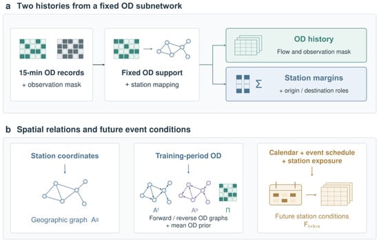
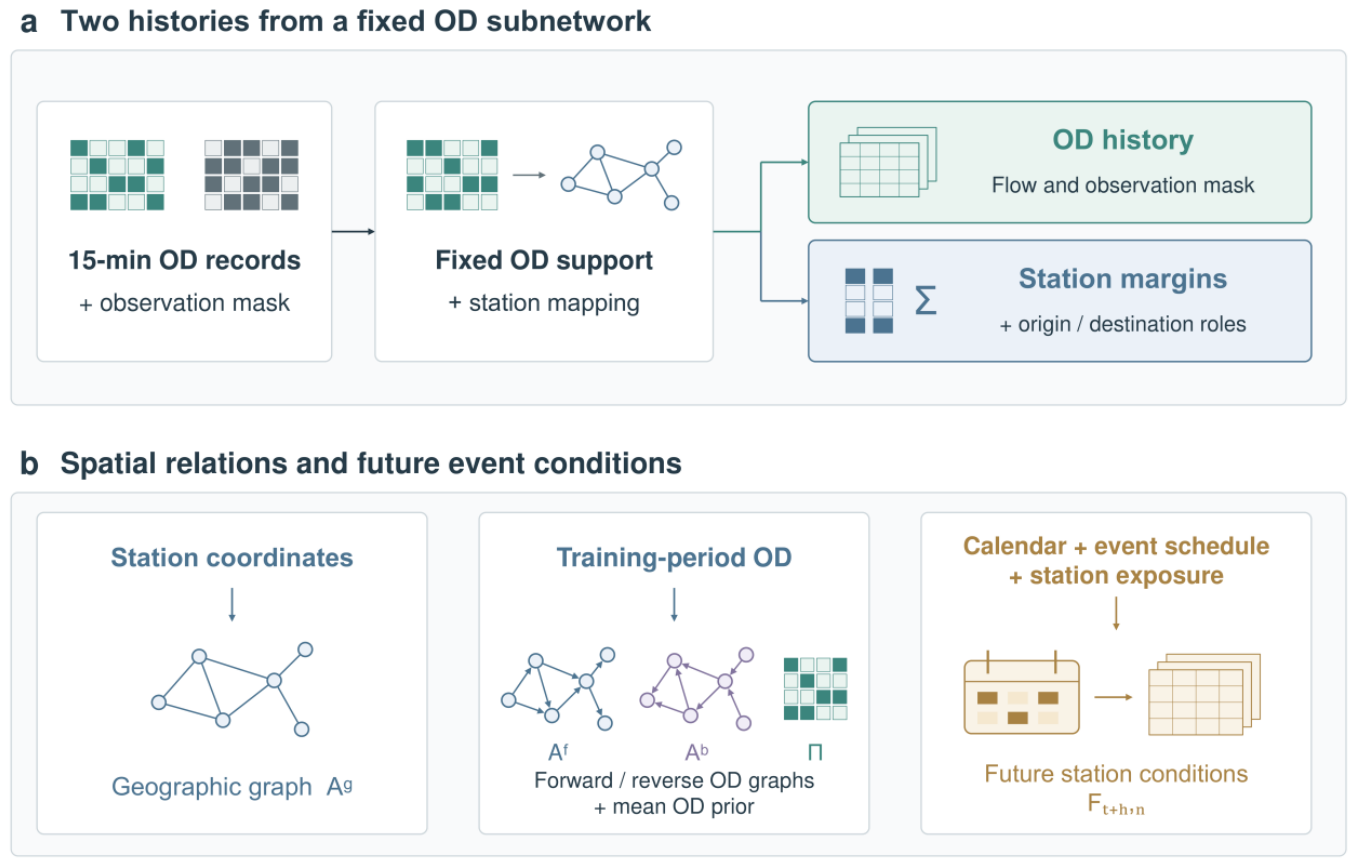
Figure 1 shows the construction of the two historical granularities, static relationships, and future conditions. OD support is determined from the earliest shared training period and then fixed. Section 2.3 defines the calculation and update rules for graph relationships and mean priors.

Figure 1. Construction of historical inputs and conditioning information.

2.2. Conditional Dual-Stream Encoding

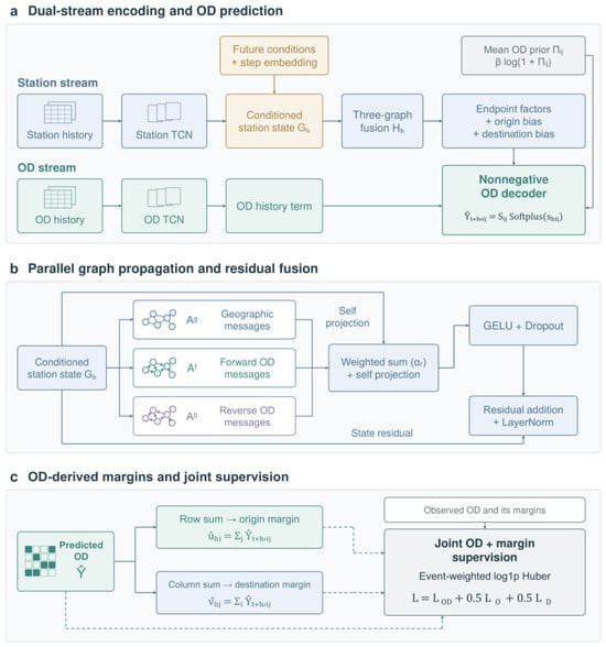
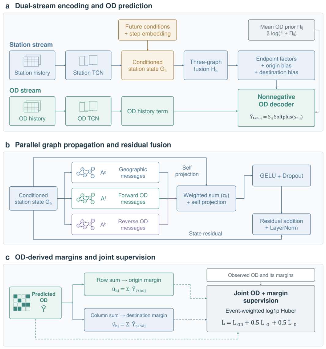
The station stream encodes changes shared across stations, while the OD stream encodes the temporal behavior of individual relationships. Shared states and relationship-specific changes therefore contribute jointly to prediction. The two branches have separate parameters, with each branch sharing parameters among entities of the same type. Residual dilated convolutions [27] capture temporal changes within the finite history, and each branch uses the hidden representation at its final historical time step. TCN in Figure 2 denotes a temporal convolutional network. The encoding shown in Figure 2 corresponds to Equation (3), with fixed layer settings in Table 3:

$$E^{\left(l\right)}=E^{(l-1)}+\mathrm{D}\mathrm{r}\mathrm{o}\mathrm{p}\left\{\mathrm{G}\mathrm{E}\mathrm{L}\mathrm{U}\right[\mathrm{G}\mathrm{N}\left({\mathrm{C}\mathrm{o}\mathrm{n}\mathrm{v}}_{3,d_l}^{\mathrm{l}\mathrm{e}\mathrm{f}\mathrm{t}}\right(E^{(l-1)}\left)\right)\left]\right\}$$

(3)

Figure 2. DMG-STNet architecture.

GELU in Equation (3) denotes the Gaussian error linear unit. Group normalization (GN) normalizes over all 8 historical steps, whose observations precede forecast issuance. The model generates four steps in one pass and learns a representation for each step through parallel supervision.

Event schedules supplement recent flow histories with information about future intervals. The model adds an encoding of the future conditions $F_{t+h,n}$ to the station-history representation so that each prediction step receives event information for its time and station:

$$G_{hn}=h_n+\mathrm{D}\mathrm{r}\mathrm{o}\mathrm{p}\left\{\mathrm{G}\mathrm{E}\mathrm{L}\mathrm{U}\right(W_F{F}_{t+h,n}+b_F\left)\right\}+e_h$$

(4)

Future conditions enter only the station stream. The OD stream retains relationship histories without graph propagation. Decoding combines recent OD changes with future event schedules, while the event table supplies conditioning features such as schedules and spatial exposure.

The confidence values in Table 3 follow the stated rules. The size proxy comes from venue capacity or other event statistics; the two Bird’s Nest concerts in this study use venue capacity. Size, exposure, and confidence are assigned within the relevant event-related windows. The value of 0.5 for Beitucheng is an exposure parameter. Event links also participate in generating arrival/departure indicators, while loss weighting follows the event-factor rule in Table 4.

2.3. Multi-Graph Propagation

The station branch combines geographic, forward-OD, and reverse-OD graphs to use both geographic proximity and travel connections across stations. The geographic graph uses Haversine distances $d_{nm}$ calculated from station coordinates. For each station, the 4 nearest other stations are selected, and the median of the selected positive distances defines bandwidth $\sigma$:

$$B_{nm}=\mathbf{1}\{m\in {\mathcal{N}}_4(n)\}\mathrm{e}\mathrm{x}\mathrm{p}(-{\displaystyle \frac{d_{nm}^2}{2{\sigma }^2}})$$

(5)

$$A_{nm}^g=max(B_{nm},B_{mn})$$

(6)

$$A_{nn}^g=0$$

(7)

The bold 1 in Equation (5) denotes the indicator function. This graph describes geographic proximity between stations. For the directional relationships, valid observed OD flows accumulated over the training period ${\mathcal{T}}_g$ of the current fitting stage are mapped to a physical-station matrix $C$. The two graphs are then constructed as:

$$A^f=\mathcal{R}\left[\mathrm{l}\mathrm{o}\mathrm{g}\right(1+C\left)\right]$$

(8)

$$A^b=\mathcal{R}\left[\mathrm{l}\mathrm{o}\mathrm{g}\right(1+C^{\mathsf{T}}\left)\right]$$

(9)

$\mathcal{R}$ divides each nonempty row by its row sum and leaves empty rows at zero. The reverse graph is obtained by transposing the unnormalized matrix and normalizing it again. It therefore generally differs from the direct transpose of the forward graph. The historical prior ${\Pi }_{ij}$ is the mean OD flow over valid observations in the training period of the same fitting stage. Hyperparameter selection uses the initial training days. For final fitting, the graphs and priors are rebuilt after the validation day is added. They remain fixed within each stage, and no test flows enter their calculation. Event-related changes are represented through historical inputs, future conditions, and learned parameters. Graph weights are not rebuilt over time during prediction.

To combine complementary relationships, each graph is clipped to nonnegative weights, augmented with unit self-loops, and row-normalized within the model, yielding ${\overline{A}}^r$. Three global parameters $a_r$ determine the shared fusion weights and the update:

$${\alpha }_r={\displaystyle \frac{\mathrm{e}\mathrm{x}\mathrm{p}\left(a_r\right)}{{\sum }_{q\in \{g,f,b\}}\mathrm{e}\mathrm{x}\mathrm{p}\left(a_q\right)}}$$

(10)

$$T_h=G_h{W}_0+b_0+{\sum }_{r\in \{g,f,b\}}{\alpha }_r{\overline{A}}^r{G}_h{W}_r$$

(11)

The fused station representation is:

$$H_h=\mathrm{L}\mathrm{N}\{G_h+\mathrm{D}\mathrm{r}\mathrm{o}\mathrm{p}[\mathrm{G}\mathrm{E}\mathrm{L}\mathrm{U}\left(T_h\right)\left]\right\}$$

(12)

LN in Equation (12) denotes layer normalization. The three shared graph weights control the contribution of each relationship type. Matrix multiplication aggregates other stations’ representations according to travel connections, combining information from different sources in each station state.

2.4. Jointly Supervised OD Decoding

The decoder adds station interactions to the OD-history term so that information shared across stations and recent changes in each OD pair jointly determine the forecast. Let $\iota \left(i\right)$ and $ȷ\left(j\right)$ map the 31 origins and 32 destinations to the unified index of 42 physical stations. Origin and destination representations are extracted from the corresponding rows of $H_h$. Separate affine transformations produce R-dimensional endpoint factors $p_{hi}$ and $q_{hj}$ ($R=8$) and the corresponding biases. A single mapping of $z_{ij}$ yields the historical contributions $b_{hij}^{\mathrm{h}\mathrm{i}\mathrm{s}\mathrm{t}}$ for all four steps:

$$s_{hij}={\displaystyle \frac{p_{hi}^{\mathsf{T}}{q}_{hj}}{\sqrt{R}}}+b_{hi}^O+b_{hj}^D+b_{hij}^{\mathrm{h}\mathrm{i}\mathrm{s}\mathrm{t}}+\beta \mathrm{l}\mathrm{o}\mathrm{g}(1+{\Pi }_{ij})+b_{\ast }$$

(13)

The prediction and activation function are defined as:

$${\hat{Y}}_{t+h,ij}=S_{ij}\mathrm{S}\mathrm{o}\mathrm{f}\mathrm{t}\mathrm{p}\mathrm{l}\mathrm{u}\mathrm{s}\left(s_{hij}\right)$$

(14)

$$\mathrm{S}\mathrm{o}\mathrm{f}\mathrm{t}\mathrm{p}\mathrm{l}\mathrm{u}\mathrm{s}\left(\mathrm{x}\right)=\mathrm{l}\mathrm{o}\mathrm{g}(1+\mathrm{e}\mathrm{x}\mathrm{p}x)$$

(15)

The factor inner product parameterizes endpoint interactions at low rank. The final output also incorporates the history term, prior, nonlinearity, and structural mask. Softplus directly produces nonnegative predictions on the original count scale, without an exponential inverse transformation. The structural mask sets invalid positions to zero.

To eliminate summation discrepancies among independently parameterized outputs, origin and destination margins are obtained directly by summing the same OD output:

$${\hat{u}}_{hi}={\sum }_j{\hat{Y}}_{t+h,ij}$$

(16)

$${\hat{v}}_{hj}={\sum }_i{\hat{Y}}_{t+h,ij}$$

(17)

$${\sum }_i{\hat{u}}_{hi}={\sum }_j{\hat{v}}_{hj}$$

(18)

Equations (16)–(18) ensure summation consistency between subnetwork OD flows and their derived margins within floating-point precision. Equations (19)–(21) supervise prediction errors against observed OD flows and margins to optimize the accuracy of travel allocation and aggregate demand, respectively.

Joint supervision of OD cells and station margins optimizes both travel allocation and demand at core stations. Dashed lines in Figure 2c denote supervision paths. A Huber loss in log space [28] is used at the OD, origin, and destination levels. With $e=\mathrm{l}\mathrm{o}\mathrm{g}(1+\hat{y})-\mathrm{l}\mathrm{o}\mathrm{g}(1+y)$ and threshold $\delta =1$, the loss is:

$${\mathcal{l}}_{\delta }(e)=\left\{\begin{array}{cc}{\displaystyle \frac{1}{2}}{e}^2,& \left|e\right|\le \delta ,\\ \delta (|e|-{\displaystyle \frac{1}{2}}\delta ),& \left|e\right|>\delta \end{array}\right.$$

(19)

For level $a\in \{\mathrm{O}\mathrm{D},O,D\}$, let $\nu$ index the batch, prediction step, and corresponding unit. The loss is normalized by the valid weights:

$$L_a={\displaystyle \frac{{\sum }_{\nu }{m}_{\nu }^a{w}_{\nu }^a{\mathcal{l}}_{\delta }\left(e_{\nu }^a\right)}{{\sum }_{\nu }{m}_{\nu }^a{w}_{\nu }^a}}$$

(20)

$$L=L_{\mathrm{O}\mathrm{D}}+0.5L_O+0.5L_D$$

(21)

OD supervision requires a structurally valid position with a known, finite target. Marginal supervision requires at least one valid pair in the row or column and known observations for every valid pair, preventing incomplete aggregates from introducing downward-biased targets. Table 4 specifies the weights, where $m_{\nu }^a$ is the valid-supervision mask and $w_{\nu }^a$ is the product of the base and event weights. Loss weighting changes samples’ influence on training, while conditioning inputs supply event information. Disabling each separately tests the roles of the optimization objective and input information.

Table 4. Shared training settings and hierarchical loss.

Item	Setting
Optimizer	AdamW [29], batch size 32, weight decay 0.0001, and gradient-norm clipping at 5
Candidates and stopping	Station/baseline hidden dimension 32 or 64, learning rate 0.001 or 0.0005. Maximum 120 epochs, patience 20, and relative validation weighted absolute percentage error (WAPE) improvement threshold 0.002
Loss levels	Huber loss in log(1 + x) space with threshold 1. OD, origin, and destination coefficients are 1.0, 0.5, and 0.5
Base weights	A weight of 1 for observed zero targets and 1.5 for positive targets. Each level is normalized by the sum of valid weights
Event factor	An additional factor of 2 when either OD endpoint is in a concert arrival or departure window. Each margin uses the maximum event factor among its valid OD pairs
Randomness	All four deep model types are fitted independently with seeds 2024, 2025, and 2026. Each deterministic baseline is run once per date
Runtime environment	Python 3.12.14, PyTorch 2.14.0 + cu126, CUDA 12.6, NVIDIA RTX 4060 Laptop GPU

Table 4. Shared training settings and hierarchical loss.

Item	Setting
Optimizer	AdamW [29], batch size 32, weight decay 0.0001, and gradient-norm clipping at 5
Candidates and stopping	Station/baseline hidden dimension 32 or 64, learning rate 0.001 or 0.0005. Maximum 120 epochs, patience 20, and relative validation weighted absolute percentage error (WAPE) improvement threshold 0.002
Loss levels	Huber loss in log(1 + x) space with threshold 1. OD, origin, and destination coefficients are 1.0, 0.5, and 0.5
Base weights	A weight of 1 for observed zero targets and 1.5 for positive targets. Each level is normalized by the sum of valid weights
Event factor	An additional factor of 2 when either OD endpoint is in a concert arrival or departure window. Each margin uses the maximum event factor among its valid OD pairs
Randomness	All four deep model types are fitted independently with seeds 2024, 2025, and 2026. Each deterministic baseline is run once per date
Runtime environment	Python 3.12.14, PyTorch 2.14.0 + cu126, CUDA 12.6, NVIDIA RTX 4060 Laptop GPU

The event factor multiplies the positive-target base weight, giving a maximum effective weight of 3. All deep comparison models share these loss and training rules. Their specific architectures and input processing are described in Section 3. Each model independently selects its width, learning rate, and number of training epochs from validation results.

3. Experimental Design

3.1. Training Configuration

The main experiments use a fixed setting of 8 historical steps (120 min) and four-step parallel supervision. Four-step training jointly learns representations for the prediction steps over the next hour, while the formal comparison focuses on the next 15 min. Section 4.3.3 independently fits 4-, 8-, and 12-step history configurations using common sample start times; their station-aggregate weighted absolute percentage error (WAPE) values are 28.55%, 28.12%, and 28.81%, respectively. The 8-step configuration has a lower mean error among the settings examined. The sample-start protocols for this sensitivity comparison and the main experiments are reported separately.

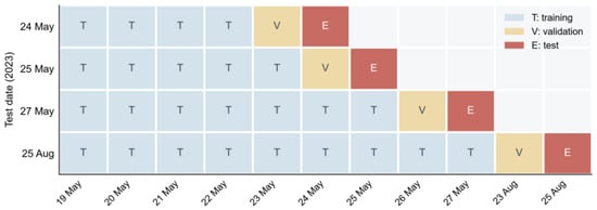
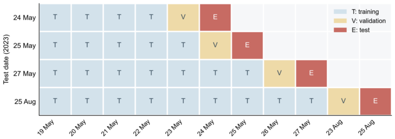
The experiments use the four test days in Table 5 and Figure 3, comprising two ordinary days and two event days. Hyperparameters are selected and models fitted separately for each date. The date axis in Figure 3 lists the available observation days, with T, V, and E denoting training, validation, and test data. Deep models first compare combinations of hidden dimension and learning rate using random seed 2024. The configuration is selected by validation WAPE over all 984 OD pairs and four supervised steps. The number of epochs is then determined separately for each training seed. Finally, the model is reinitialized with the corresponding seed and fitted on the combined training and validation days. For the main-comparison models, seed 2024 reuses the validated epoch count of the selected candidate configuration. Test targets do not enter parameter selection, and each date is fitted independently.

Table 5. Date splits and final DMG-STNet settings for the four target days.

Test Day	Initial Training Days	Validation Day	Final Fitting Days	Width	Epochs for the Three Seeds
24 May 2023	19–22 May 2023	23 May 2023	19–23 May 2023	32	94/95/56
25 May 2023	19–23 May 2023	24 May 2023	19–24 May 2023	32	114/108/115
27 May 2023	19–25 May 2023	26 May 2023	19–26 May 2023	64	118/119/117
25 August 2023	19–27 May 2023	23 August 2023	19–27 May 2023 and 23 August 2023	64	117/109/107

Note: The learning rate is 0.001. Epoch counts correspond to seeds 2024, 2025, and 2026, in that order.

Figure 3. Date splits for the four test days.

Independent TCN, OD-STGCN, Graph WaveNet, and DMG-STNet are each run independently with random seeds 2024, 2025, and 2026. Before each fit, the random states of Python, NumPy, and PyTorch are set. The same seed controls parameter initialization and training-sample shuffling. Historical Average and Pairwise Ridge are deterministic and are run once per date. The software environment used Python 3.12.14 (Python Software Foundation, Beaverton, OR, USA; https://www.python.org/), PyTorch 2.14.0+cu126 (https://pytorch.org/), and CUDA 12.6 (NVIDIA Corporation, Santa Clara, CA, USA). Additional library versions were NumPy 2.5.2 (https://numpy.org/), pandas 3.0.5 (https://pandas.pydata.org/), Matplotlib 3.11.1 (https://matplotlib.org/), SciPy 1.18.1 (https://scipy.org/), and scikit-learn 1.9.0 (https://scikit-learn.org/).

The fitting data for 27 May include earlier event observations, while the final fit for 25 August includes 23 August. These data allow the model to learn historical event patterns and incorporate information from recent dates for calibration. The main setting yields 67 windows per complete training day and 70 windows per target day. Daily linked-OD results are calculated over the full daily evaluation period for each of the four dates. The event-window union and arrival/departure-window union are additionally selected for focused evaluation on the two event days. Future calendar and event features needed for forecasts near the end of the day are generated along the time axis. Four-step training and evaluation for the next 15 min use their respective target-availability conditions.

The experiments use an NVIDIA GeForce RTX 4060 Laptop GPU (NVIDIA Corporation, Santa Clara, CA, USA). The event-day configurations in Table 5 contain 44,483 trainable parameters, while the ordinary-day configurations contain 12,259. For the existing configuration with 44,483 parameters, efficiency measurements used GPU-synchronized timing of 100 consecutive forward passes after 5 warm-up passes. Forward-pass latency was 3.36 ms for a single sample and 3.18 ms for a complete batch of 32 samples, both averaged across the three seeds; the maximum peak allocated GPU memory was 64.35 MiB. Each sample produces four OD matrices in one pass. These times cover model forward computation and exclude data reading, preprocessing, and service communication.

3.2. Comparison Models

Six model types are included: Historical Average (HA), Pairwise Ridge, Independent TCN, OD-STGCN, Graph WaveNet, and DMG-STNet. They represent intraday averaging, pairwise linear regression, OD temporal convolution, station graph convolution, adaptive graph relationships, and the dual-stream multi-graph design, respectively. Table 6 summarizes their information scope and fitting procedures. The comparison implementations follow the corresponding methodological ideas in the literature, with graph baselines adapted to OD forecasting for this task.

Table 6. Comparison models and their implementations for this task.

Model	Information and Architecture	Fitting and Adaptation
HA [13,30]	Historical mean for each OD pair in the same 15 min time slot	Calculated over the final fitting dates without additional day-of-week matching
Pairwise Ridge [31]	Separate regression for each OD pair and prediction step using 8 historical values on the original count scale; no future conditioning inputs	Ridge regression with nonnegative coefficients. Candidate α values: 0.1, 1, 10, 100. All four test dates select 0.1. Refitted over the final fitting period
Independent TCN [27]	A shared temporal encoder and four-step prediction head across OD pairs, without graph propagation or future conditioning inputs	Original-count and log1p versions of historical OD flows, with separate parameter selection by date and fitting by seed
OD-STGCN [11]	Station TCN, shared future conditions, geographic graph, and endpoint-factor OD decoder	Original-count and log1p versions of station flows, each with separate parameter selection and fitting. Geographic relationships are not the actual rail-network graph
Graph WaveNet [12]	Station TCN, shared future conditions, a static support obtained by averaging the three graphs, and a learnable adaptive support	Original-count and log1p versions of station flows, with 10-dimensional left and right node embeddings and separate parameter selection and fitting
DMG-STNet	Station and OD streams, three fixed graphs, shared future conditions, and decoding with history and prior terms	Historical flows use log1p inputs. Four-step supervision, with the formal comparison restricted to the next 15 min

All models predict flows for the study OD pairs over the next 15 min, using the date splits in Table 5. They are evaluated on the same OD set, time windows, and station-aggregation definitions. HA and Pairwise Ridge are fitted by their respective deterministic procedures. The four deep model types share the three-level event-weighted Huber loss, candidate set, stopping rules, and training seeds. The main comparison retains original-count inputs for the three deep baselines and log(1 + x) inputs for DMG-STNet. Supplementary comparisons apply log(1 + x) to the historical OD-flow channels of Independent TCN and the historical station-flow channels of OD-STGCN and Graph WaveNet; masks, roles, calendar channels, and event channels retain their original values. Targets remain on the original count scale, outputs are nonnegative counts, and losses are still calculated in log space according to Equations (19)–(21).

For each of the four dates, each log1p baseline searches the original four-configuration grid with seed 2024, then determines the epoch count and performs an independent final fit with each of seeds 2024, 2025, and 2026. Seed 2024 reuses the epoch count of the corresponding selected candidate. Results for all test dates are reported separately for the original-count and log1p input versions. OD-STGCN, Graph WaveNet, and DMG-STNet use the same future calendar and event conditions. Independent TCN does not use future conditioning inputs for prediction but shares the event-weighted training loss. HA uses historical means for the same time slot, and Pairwise Ridge has no future conditioning inputs. Comparisons with Independent TCN or Pairwise Ridge therefore reflect the combined effects of information configuration and model structure. The common-transformation comparison examines each complete implementation’s sensitivity to historical-flow processing; differences between input versions also include the effects of renewed parameter selection and adaptation.

3.3. Experimental Settings

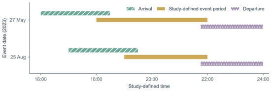
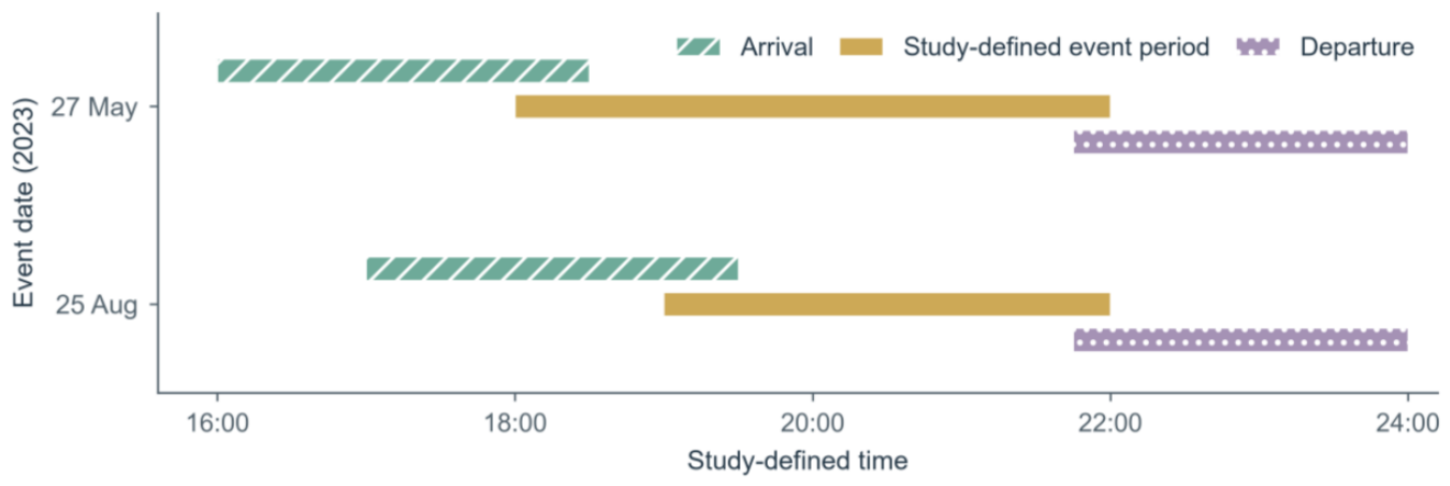
For all four test days, daily results for the 122 OD pairs linked to the core stations are calculated over the full daily evaluation period to assess linked-OD forecasting on ordinary and event days. The main evaluation focuses on the event windows of 27 May and 25 August 2023, examining both linked OD flows and their station-direction aggregates. The event-window union covers arrivals, the event itself, and departures. The arrival/departure-window union focuses on the two phases with concentrated changes in demand. All windows include their left endpoint and exclude their right endpoint, and overlaps are counted once. Table 7 gives the schedules, windows, and station-direction sample counts, while Figure 4 shows the evaluation windows. Arrival/departure windows are defined from event schedules recorded in advance. Each time slot contains four samples, comprising two stations and two directions. The arrival/departure-window union contains 19 time slots and 76 samples on each event day. Across both event days, the event-window union and arrival/departure-window union contain 240 and 152 station-direction samples, respectively.

Table 7. Study-defined event periods, evaluation windows, and station-direction sample counts on the event days.

Date	Study-Defined Event Period	Arrival Window	Departure Window	Station-Direction Samples in the Event-Window Union
27 May 2023	18:00–22:00	16:00–18:30	21:45–24:00	128
25 August 2023	19:00–22:00	17:00–19:30	21:45–24:00	112

Figure 4. Evaluation windows for the two event days.

Based on the start and end times recorded in the event and venue information workbook, the study-defined event periods were set to 18:00–22:00 on 27 May and 19:00–22:00 on 25 August for constructing event features and evaluation windows. Table 7 and Figure 4 retain the study settings: the event-window union is [16:00, 24:00) on 27 May and [17:00, 24:00) on 25 August, with arrival and departure windows constructed according to Table 3.

Component experiments are conducted on the two event days and report aggregate results over the event-window union for both stations and directions. Structural and event-condition configurations also report event-window-union results for the 122 linked OD pairs, while the marginal-supervision control additionally reports OD errors over the arrival/departure-window union. Table 8 defines the experimental treatments. Structural and event-related variants requiring refitting use the width and learning rate selected for the full model on the corresponding date but determine their epoch counts independently. The history-length experiment uses common sample start times with a complete 12-step history and the corresponding valid targets, from which 4-, 8-, and 12-step inputs are extracted. Common start times are determined separately for training, validation, and testing under the original date splits. Each complete training day provides 63 windows, and each test day provides 66 windows with target start times from 07:30 to 23:45. All three history configurations are fitted independently. The event evaluation windows lie entirely within this shared range, retaining 240 evaluation samples.

Table 8. Definitions of component and sensitivity experiments.

Experiment	Treatment	Model Weights Refitted?
Structure	Replace geographic relationships with self-loops, replace forward/reverse-OD relationships with self-loops, disable the OD-history decoding term, disable marginal loss, or set the decoding rank to 4	Yes, for each variant and seed
Event conditions	A00: both disabled. A10: event inputs only. A01: event weighting only. A11: both inputs and weighting enabled	Yes for A00/A10/A01. A11 reuses the full model
History length	Extract 4-, 8-, and 12-step inputs at common start times with a complete 12-step history and corresponding valid targets	Yes, including the 8-step configuration
Perturbations with fixed weights	Set event channels to zero, shift the entire schedule 60 min later and re-encode it, or construct a full-day permutation using seed 76,123 and the date	No. Use full-model weights from the corresponding seed

Refitted controls compare configurations after training, while inference perturbations assess the dependence of a fixed model on its inputs. Event weighting uses the arrival and departure masks. For intraday shuffling, the perturbation seed 76,123 is added to the eight-digit integer representation of the target date to generate a fixed random permutation of the day’s 96 15 min intervals. Event conditions are mapped before batched inference. Models from the three training seeds use the same date-specific mapping and their respective fitted weights, while calendar channels remain unchanged. The first three calendar channels are retained when event inputs are disabled or perturbed. Encoder parameters are retained when the OD-history decoding term is disabled.

3.4. Evaluation Methods

Weighted absolute percentage error (WAPE), mean absolute error (MAE), root mean squared error (RMSE), and the coefficient of determination (R²) are used. Lower values are better for the first three metrics. Higher R² is better, and negative values are possible. For N_e valid records in a given evaluation set, with observations y_k and predictions ŷ_k, the metrics are defined as:

$$\mathrm{W}\mathrm{A}\mathrm{P}\mathrm{E}={\displaystyle \frac{{\sum }_{k=1}^{N_e}|{\hat{y}}_k-y_k|}{{\sum }_{k=1}^{N_e}\left|y_k\right|}}\times 100\%$$

(22)

$$\mathrm{M}\mathrm{A}\mathrm{E}={\displaystyle \frac{1}{N_e}}{\sum }_{k=1}^{N_e}|{\hat{y}}_k-y_k|$$

(23)

$$\mathrm{R}\mathrm{M}\mathrm{S}\mathrm{E}=\sqrt{{\displaystyle \frac{1}{N_e}}{\sum }_{k=1}^{N_e}({\hat{y}}_k-y_k{)}^2}$$

(24)

$$R^2=1-{\displaystyle \frac{{\sum }_{k=1}^{N_e}{\left(y_k-{\widehat{y}}_k\right)}^2}{{\sum }_{k=1}^{N_e}{\left(y_k-\overline{y}\right)}^2}}$$

(25)

Here, $\overline{y}={\displaystyle \frac{1}{N_e}}{\sum }_{k=1}^{N_e}{y}_k$ is the mean observed value in the same evaluation set. WAPE is undefined when the total observed flow is zero, and R² is undefined when observations have no variation. MAE and RMSE are measured in trips/OD pair/15 min at the OD level and trips/study-station direction/15 min at the aggregate level.

OD evaluation uses each date-OD pair-time combination as a unit and directly compares observations and predictions for the 122 linked OD pairs. Station-level evaluation first sums observations and predictions by origin or destination, then uses each date-station-direction-time combination as a unit. Full-day OD metrics are calculated separately for each of the four test days, with 8540 records per day. Event-window results are calculated for individual days or pooled samples from both event days, with records concatenated within the same evaluation level. For every evaluation set, metrics are first calculated separately for each random seed and then summarized by the arithmetic mean and minimum-to-maximum range across the three seeds. Deterministic models report the result of a single fit. OD evaluation describes the accuracy of origin–destination relationships, while station-aggregate evaluation describes demand at stations affected by the event.

Relative improvement is calculated as (comparison-model error − DMG-STNet error)/comparison-model error × 100%. Direct differences in WAPE are expressed in percentage points.

Paired time-block resampling intervals are additionally calculated for two core comparisons over the event-window union of the two event days: DMG-STNet versus Pairwise Ridge at the OD level, and DMG-STNet versus original-input Independent TCN at the station-aggregate level. Error differences are defined as comparison-model error minus DMG-STNet error, with WAPE differences expressed in percentage points; positive values indicate lower DMG-STNet error. Records from both days are concatenated, metrics are calculated separately for each seed, and the metrics are then averaged across seeds. Deterministic Pairwise Ridge contributes its single result; predictions are not averaged before metric calculation.

Sampling is performed separately within the arrival, middle-event, and departure phases of each date, retaining 10, 13, and 9 slots on 27 May and 10, 9, and 9 slots on 25 August. Non-circular consecutive time blocks are sampled, with the last block truncated to the required length. All objects, models, and training seeds at a given time share the same sampling index. Based on the lag correlations of phase-centered paired absolute-error differences, the primary block length of 2 slots (30 min) and the adjacent length of 3 slots (45 min) are fixed before interval calculation. Each comparison and block length uses 2000 resamples, with the 2.5th and 97.5th percentiles of the difference distribution forming a two-sided approximate 95% interval. The resampling seeds for the two OD block lengths are 677,502 and 677,503, and those for station aggregates are 677,602 and 677,603. These intervals are conditional on the two events and the saved models; the minimum-to-maximum range across three training seeds separately describes training variation.

4. Prediction Results

4.1. OD Prediction

4.1.1. Prediction by Date

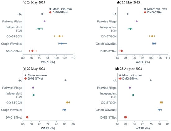
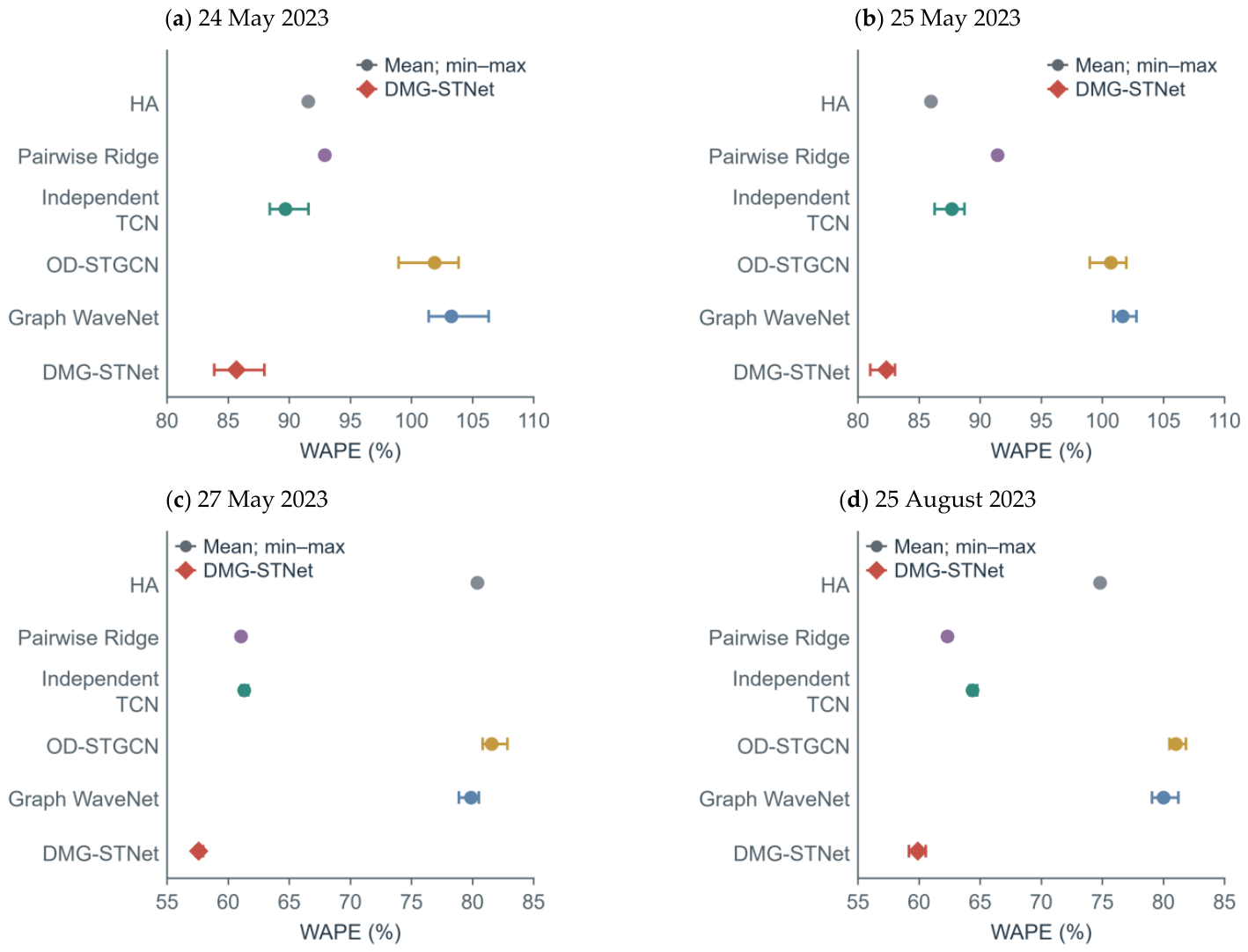
Table 9, Table 10, Table 11, Table 12 and Table 13 use the main-comparison inputs described in Section 3.2: HA, Pairwise Ridge, and the three deep baselines use original-count historical flows, while DMG-STNet uses log(1 + x) historical flows. Figure 5 and Table 9 and Table 10 report prediction results for the 122 linked OD pairs from 06:30 to 23:45 on each of the four test days. In the point-and-error-bar plots, points for the deep models denote the mean metric across three training seeds, and error bars show the minimum-to-maximum range. In Table 9 and Table 10, DMG-STNet achieves WAPE values of 85.68%, 82.32%, 57.58%, and 59.91% on 24 May, 25 May, 27 May, and 25 August, respectively; its MAE and RMSE are also lower than those of the other five model types. For OD results in this paper, MAE and RMSE are measured in trips/OD pair/15 min, and R² is dimensionless.

Table 9. Prediction metrics for linked OD pairs on the two ordinary days.

Date	Model	WAPE/%	MAE	RMSE	R2
24 May 2023	HA	91.55	0.964	1.900	0.344
24 May 2023	Pairwise Ridge	92.89	0.978	1.876	0.360
24 May 2023	Independent TCN	89.69	0.944	2.036	0.246
24 May 2023	OD-STGCN	101.89	1.072	2.138	0.169
24 May 2023	Graph WaveNet	103.25	1.087	2.129	0.176
24 May 2023	DMG-STNet	85.68	0.902	1.852	0.376
25 May 2023	HA	85.98	0.919	1.846	0.377
25 May 2023	Pairwise Ridge	91.42	0.977	1.820	0.394
25 May 2023	Independent TCN	87.69	0.937	1.873	0.359
25 May 2023	OD-STGCN	100.68	1.076	2.071	0.215
25 May 2023	Graph WaveNet	101.66	1.086	2.066	0.219
25 May 2023	DMG-STNet	82.32	0.880	1.780	0.420

Table 10. Prediction metrics for linked OD pairs on the two event days.

Date	Model	WAPE/%	MAE	RMSE	R2
27 May 2023	HA	80.38	2.702	7.183	0.235
27 May 2023	Pairwise Ridge	61.05	2.052	4.540	0.694
27 May 2023	Independent TCN	61.30	2.060	4.719	0.670
27 May 2023	OD-STGCN	81.57	2.742	7.319	0.205
27 May 2023	Graph WaveNet	79.87	2.685	7.080	0.256
27 May 2023	DMG-STNet	57.58	1.936	4.424	0.710
25 August 2023	HA	74.80	2.566	6.950	0.268
25 August 2023	Pairwise Ridge	62.33	2.138	4.920	0.633
25 August 2023	Independent TCN	64.36	2.208	5.306	0.573
25 August 2023	OD-STGCN	81.01	2.779	7.116	0.232
25 August 2023	Graph WaveNet	80.01	2.745	6.953	0.267
25 August 2023	DMG-STNet	59.91	2.055	4.810	0.649

Table 11. Prediction metrics for OD pairs linked to the core stations on the two event days.

Evaluation Window	Model	WAPE/%	MAE	RMSE	R2
Event-window union	HA	76.39	3.664	8.991	0.218
Event-window union	Pairwise Ridge	56.48	2.709	5.614	0.695
Event-window union	Independent TCN	56.99	2.733	5.893	0.664
Event-window union	OD-STGCN	78.50	3.765	9.186	0.184
Event-window union	Graph WaveNet	76.84	3.686	8.956	0.224
Event-window union	DMG-STNet	52.94	2.539	5.318	0.726
Arrival/departure-window union	HA	74.77	3.797	9.787	0.213
Arrival/departure-window union	Pairwise Ridge	55.00	2.793	6.065	0.698
Arrival/departure-window union	Independent TCN	55.87	2.838	6.433	0.660
Arrival/departure-window union	OD-STGCN	77.34	3.928	9.985	0.180
Arrival/departure-window union	Graph WaveNet	75.51	3.835	9.725	0.223
Arrival/departure-window union	DMG-STNet	50.46	2.563	5.740	0.729

Table 12. Prediction metrics for core stations within the event-window union on the two event days.

Date	Model	WAPE/%	MAE	RMSE	R2
27 May 2023	HA	65.08	103.84	183.03	0.027
27 May 2023	Pairwise Ridge	30.37	48.46	78.01	0.823
27 May 2023	Independent TCN	25.95	41.41	67.76	0.867
27 May 2023	OD-STGCN	60.41	96.40	172.87	0.130
27 May 2023	Graph WaveNet	55.95	89.27	160.20	0.253
27 May 2023	DMG-STNet	24.40	38.93	67.57	0.866
25 August 2023	HA	63.30	90.01	142.66	0.163
25 August 2023	Pairwise Ridge	28.71	40.82	55.63	0.873
25 August 2023	Independent TCN	25.00	35.55	54.06	0.880
25 August 2023	OD-STGCN	48.17	68.49	124.53	0.362
25 August 2023	Graph WaveNet	45.40	64.55	115.40	0.449
25 August 2023	DMG-STNet	23.54	33.47	48.13	0.905

Table 13. Pooled station prediction metrics for the two window sets.

Model	Event-Window Union WAPE/% Mean (Range)	Arrival/Departure-Window Union WAPE/%	Event-Window Union MAE	Event-Window Union RMSE	Event-Window Union R2
HA	64.30(64.30–64.30)	64.16	97.39	165.42	0.081
Pairwise Ridge	29.64(29.64–29.64)	29.68	44.89	68.48	0.843
Independent TCN	25.53(25.16–25.76)	25.97	38.67	61.75	0.872
OD-STGCN	55.05(51.96–58.24)	58.03	83.38	152.25	0.221
Graph WaveNet	51.33(48.44–53.98)	53.97	77.74	141.16	0.330
DMG-STNet	24.02(23.55–24.91)	23.04	36.38	59.44	0.881

Figure 5. Weighted absolute percentage error (WAPE) for linked OD predictions on the four test days.

4.1.2. Prediction Within Event Windows

Table 11 evaluates the 122 OD pairs linked to the core stations on the two event days. The event-window union and arrival/departure-window union contain 7320 and 4636 OD-interval records, respectively. DMG-STNet achieves WAPE values of 52.94% and 50.46%. For the event-window union, MAE, RMSE, and R² are 2.539 trips/OD pair/15 min, 5.318 trips/OD pair/15 min, and 0.726, respectively. Relative to Pairwise Ridge, the baseline with the lowest WAPE in both window sets, DMG-STNet reduces WAPE by 6.27% and 8.24%, respectively. Section 4.2.1 presents the paired error differences and intervals relative to Pairwise Ridge over the event-window union. Bold text in Table 11 highlights DMG-STNet and its results.

4.2. Station-Level Aggregate Prediction

4.2.1. Errors Within Event Windows

Table 12 reports prediction results for the next 15 min for the core stations within the event-window union on the two event days. DMG-STNet achieved WAPE values of 24.40% on 27 May and 23.54% on 25 August, representing relative reductions of 5.99% and 5.84% from the 25.95% and 25.00% achieved by Independent TCN with raw-count inputs. The corresponding MAE values were 38.93 and 33.47 trips/study-station direction/15 min, and RMSE values were 67.57 and 48.13 trips/study-station direction/15 min. All subsequent station-level MAE and RMSE results use this evaluation unit; R² is dimensionless.

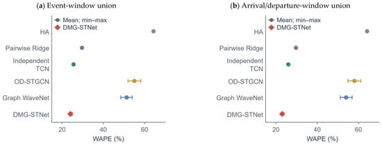
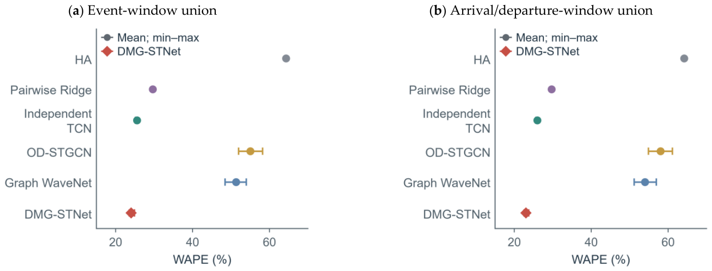
Figure 6 and Table 13 pool the core-station origin and destination samples from the two event days. DMG-STNet achieved WAPE values of 24.02% for the event-window union and 23.04% for the arrival/departure-window union, representing relative reductions of 5.92% and 11.28%, respectively, from Independent TCN with raw-count inputs.

Figure 6. Prediction WAPE for the core stations.

Table 13 reports MAE, RMSE, R² and the WAPE seed range for the event-window union. DMG-STNet achieved an MAE of 36.38 trips/study-station direction/15 min, an RMSE of 59.44 trips/study-station direction/15 min and an R² of 0.881. Its WAPE ranged from 23.55% to 24.91% across the three seeds, compared with 25.16% to 25.76% for Independent TCN with raw-count inputs. Deep models are reported by their mean metrics across three seeds and minimum–maximum ranges; deterministic HA and Pairwise Ridge use a single result each. The seed ranges describe training variability in these runs, while paired time-block intervals are reported later in this section.

The two evaluation levels describe errors at different granularities: station-aggregate WAPE for the event-window union is 24.02%, compared with a pooled WAPE of 52.94% for the 122 linked OD pairs. Positive and negative errors across OD pairs can cancel during aggregation, so lower station-level errors indicate more accurate demand-volume estimates rather than equal accuracy for every OD pair. The value of 52.94% is a pooled metric for the same evaluation set; its reduction from Pairwise Ridge is 3.54 percentage points, or 6.27% in relative terms. These two measures of improvement are used separately.

Table 14 reports WAPE for the three deep baselines using log1p historical passenger-flow inputs, with evaluation scopes as rows and models as columns. At the OD level, it covers the full day on all four test dates and the two pooled event-window sets; at the station level, it covers the two event days and the two pooled window sets. Each cell gives the three-seed mean and minimum–maximum range. The effect of the input transformation varies by model and date: Independent TCN changes from 89.69% to 89.09% for full-day OD WAPE on 24 May and from 61.30% to 68.41% on 27 May, while both graph baselines show lower pooled station-level errors after transformation. Compared with Table 9, Table 10, Table 11, Table 12 and Table 13, DMG-STNet retains lower mean OD WAPE on all four test days and lower mean OD and station WAPE in the pooled windows of the two event days than these supplementary configurations. This comparison describes the sensitivity of each complete implementation to historical passenger-flow preprocessing.

Table 14. WAPE (%) across evaluation scopes with log1p inputs.

Evaluation Level/Date/Window	Independent TCN	OD-STGCN	Graph WaveNet
OD/24 May 2023 full day	89.09 (88.80–89.27)	101.71 (98.18–106.95)	98.44 (95.57–100.62)
OD/25 May 2023 full day	88.18 (85.16–90.38)	100.44 (96.60–104.18)	99.08 (98.57–99.83)
OD/27 May 2023 full day	68.41 (67.38–69.00)	80.49 (77.73–82.95)	77.17 (76.37–77.93)
OD/25 August 2023 full day	67.83 (67.48–68.02)	79.29 (78.51–80.26)	79.74 (79.23–80.11)
OD/two-day event-window union	64.80 (64.07–65.19)	77.59 (76.14–79.12)	75.52 (75.10–76.19)
OD/two-day arrival/departure-window union	64.25 (63.67–64.61)	75.92 (74.49–77.24)	73.18 (72.36–74.23)
Station/27 May 2023 event-window union	38.47 (36.33–40.10)	55.91 (48.31–62.46)	43.78 (38.52–48.62)
Station/25 August 2023 event-window union	29.77 (28.62–30.65)	41.00 (38.51–44.45)	38.83 (38.38–39.55)
Station/two-day event-window union	34.66 (33.84–35.07)	49.38 (46.62–51.97)	41.61 (38.97–44.22)
Station/two-day arrival/departure-window union	35.30 (34.80–35.58)	50.30 (48.19–52.12)	42.95 (40.55–45.69)

Table 15 reports paired comparisons over the event-window union of the two event days. At the OD level, DMG-STNet reduces WAPE by 3.5429 percentage points and MAE by 0.1699 trips/OD pair/15 min relative to Pairwise Ridge. The approximate 95% intervals are above zero for both the main 30 min block length and the adjacent 45 min block length, supporting lower OD errors under the present sample and statistical settings. At the station-aggregate level, the mean reductions from Independent TCN with raw-count inputs are 1.5124 percentage points in WAPE and 2.2907 trips/study-station direction/15 min in MAE. Under both block lengths, the approximate 95% intervals for the station-aggregate WAPE difference include zero. The conclusions agree between the two block lengths. The two evaluation levels use 7320 OD records and 240 station-direction records, respectively, both covering 60 time points. Each comparison uses 2000 resamples for each block length, and the intervals in the table refer to the WAPE difference.

Table 15. Paired error differences over the event-window union of the two event days.

Level/Comparison Model	Block Length	WAPE Difference/Percentage Points	Approximate 95% Interval for WAPE Difference	MAE Difference
OD/Pairwise Ridge	30 min, main analysis	3.5429	[1.2050, 5.7296]	0.1699
OD/Pairwise Ridge	45 min, adjacent block length	3.5429	[0.9215, 5.7858]	0.1699
Station/raw-input TCN	30 min, main analysis	1.5124	[−1.1801, 3.5251]	2.2907
Station/raw-input TCN	45 min, adjacent block length	1.5124	[−0.9401, 3.9690]	2.2907

4.2.2. Responses by Station Direction

Table 16 separates the main-comparison results for the event-window union by date, station and direction. DMG-STNet achieved the lowest WAPE in five of the eight combinations. For station A origin on 27 May, its WAPE was 29.88%, compared with a minimum of 31.93% among the other models. For station A destination on 25 August, the corresponding values were 12.22% and 15.99%. The comparison-model minimum uses the input versions of the five baselines in the main comparison described in Section 3.2.

Table 16. Event-window union WAPE by date, station and direction.

Date	Station	Direction	DMG-STNet/%	Lowest-WAPE Comparison Model	Minimum WAPE/%
27 May 2023	B	Destination	25.29	Pairwise Ridge	31.20
27 May 2023	B	Origin	26.60	OD-STGCN	28.27
27 May 2023	A	Destination	19.54	Independent TCN	18.72
27 May 2023	A	Origin	29.88	Independent TCN	31.93
25 August 2023	B	Destination	35.25	Graph WaveNet	40.35
25 August 2023	B	Origin	32.95	OD-STGCN	28.16
25 August 2023	A	Destination	12.22	Independent TCN	15.99
25 August 2023	A	Origin	32.57	Independent TCN	30.36

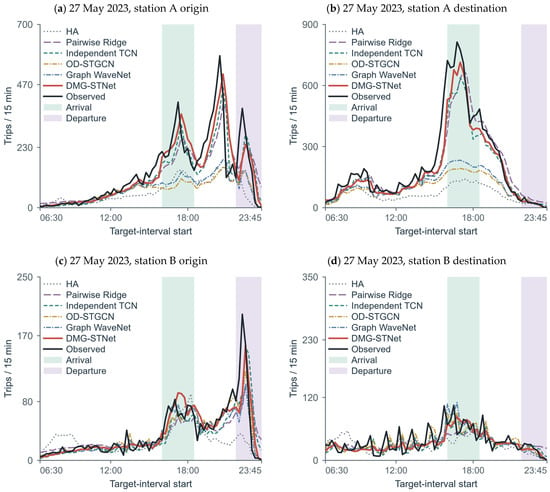
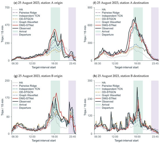
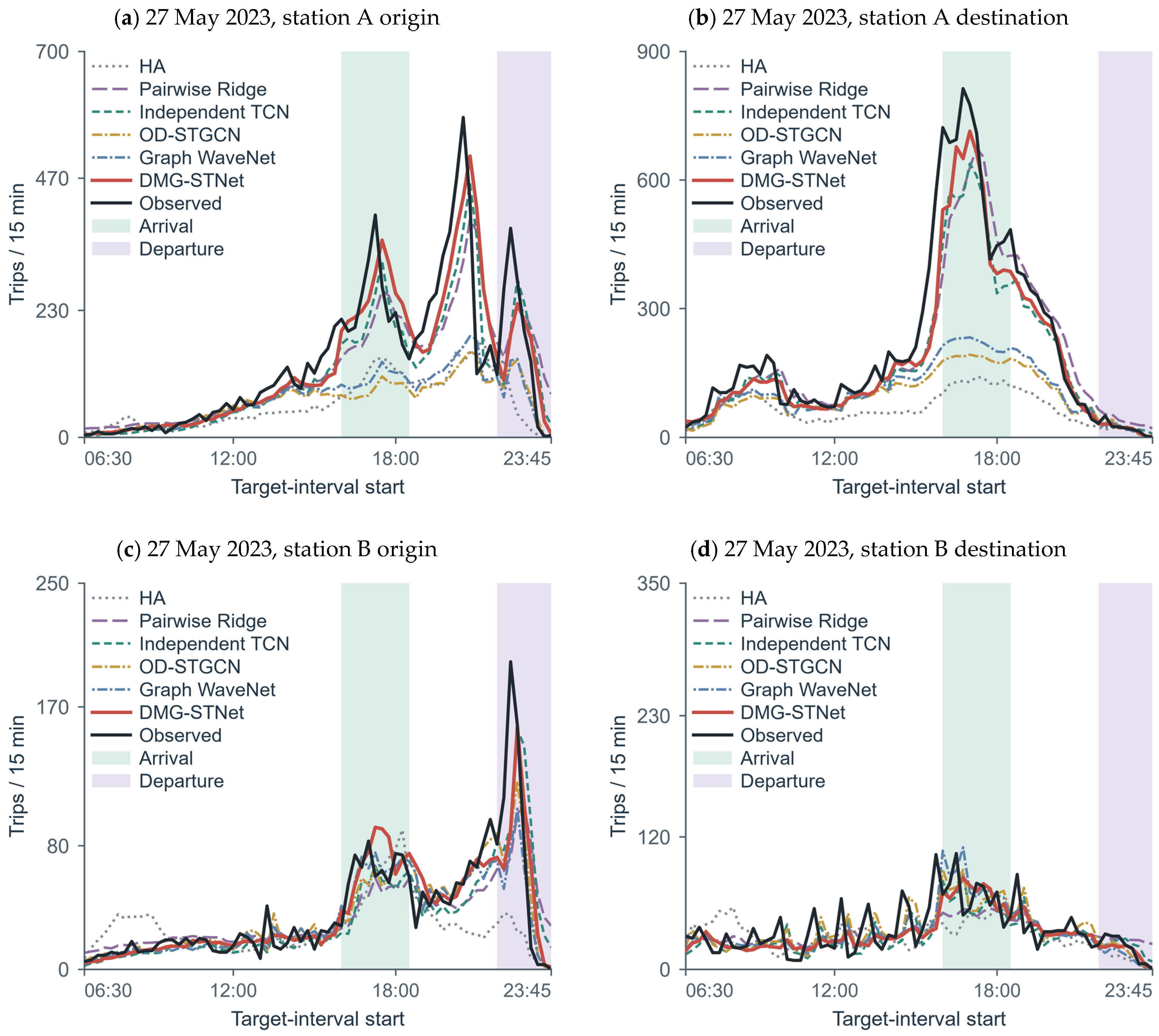
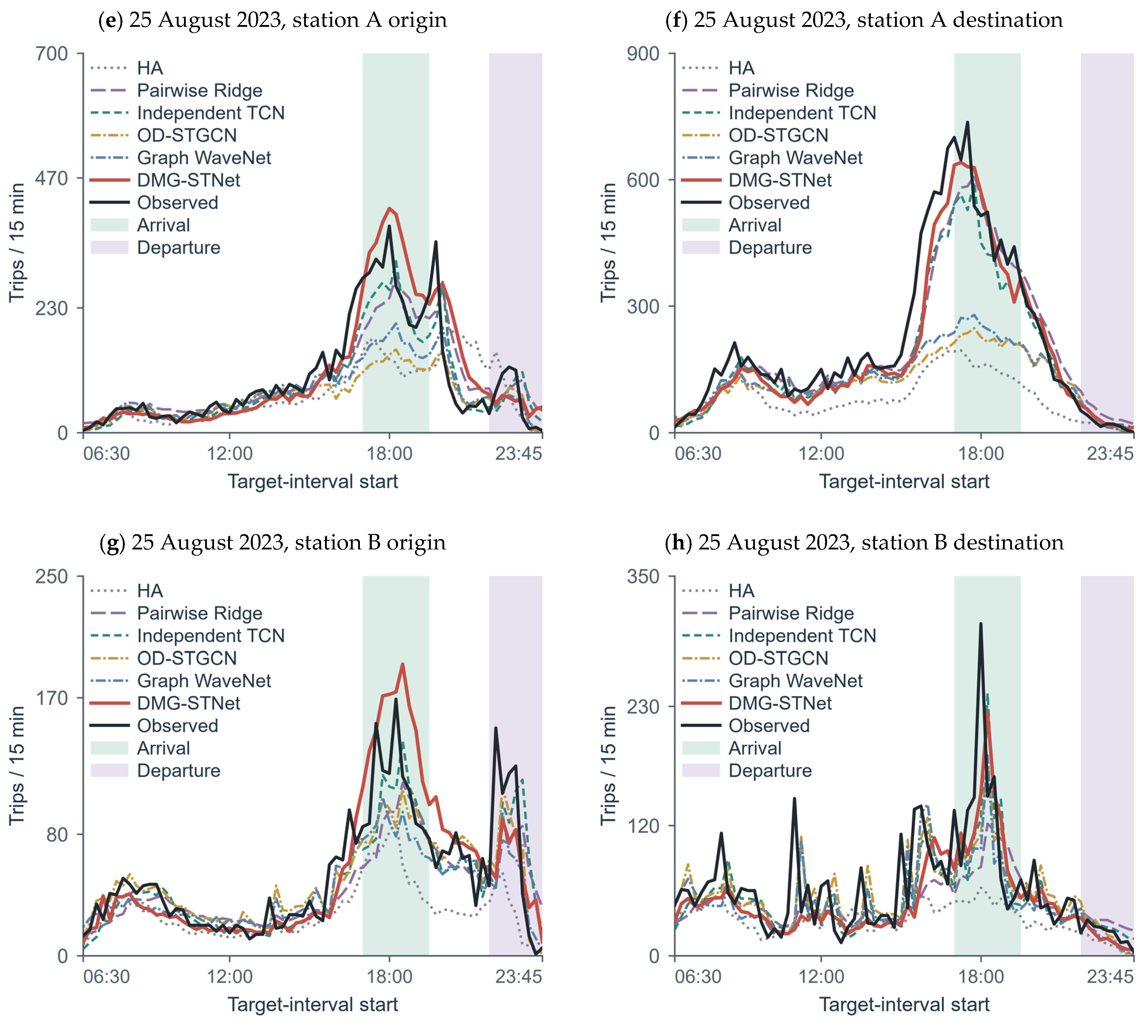
Figure 7 shows the core-station origin and destination time series from 06:30 to 23:45 on the two event days. The deep-model curves use the main-comparison results with seed 2024. Green and purple shading denote the arrival and departure windows, respectively. Increases in destination flows at station A were concentrated within the arrival window on both dates, whereas the prominent origin-flow peak at station B on 27 May occurred within the departure window.

Figure 7. Full-day prediction time series for the core stations.

4.3. Component Effects

4.3.1. Structural Ablation

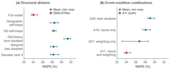
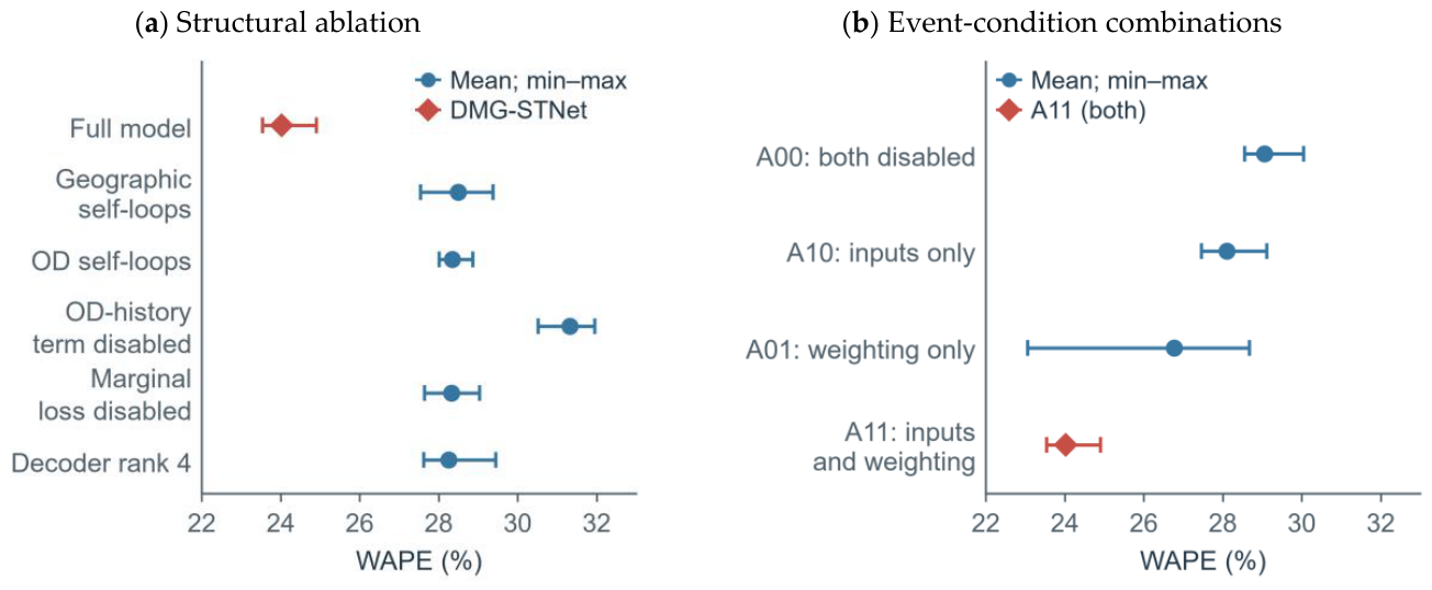
Figure 8a and Table 17 compare the full model with five refitted structural variants. On the same event-window union, the full model achieved a WAPE of 24.02%, 7.30 percentage points lower than the 31.32% obtained without the OD-history decoding term. This was the largest improvement among the structural comparisons. Directly retaining recent changes in each OD pair during decoding therefore provides useful information for predicting core-station demand volumes.

Figure 8. Component analysis for core stations within the event-window union.

Table 17. Structural ablation within the event-window union.

Model/Setting	WAPE/%	WAPE Range/%	MAE	RMSE	R2
Full model	24.02	23.55–24.91	36.38	59.44	0.881
Geographic graph reduced to self-loops	28.50	27.54–29.38	43.16	73.62	0.818
OD graphs reduced to self-loops	28.34	28.01–28.87	42.93	73.74	0.817
OD-history term disabled	31.32	30.52–31.96	47.44	82.52	0.771
Marginal loss disabled	28.32	27.65–29.03	42.89	74.46	0.814
Decoder rank 4	28.26	27.62–29.44	42.80	73.26	0.819

Reducing the geographic graph or the forward/reverse-OD graphs to self-loops yielded WAPE values of 28.50% and 28.34%, respectively. The full model reduced these errors by 4.47 and 4.32 percentage points. Both comparisons retain the corresponding branch parameters and self-loop propagation to assess the contribution of cross-station relationships. Combining geographic proximity with training-period travel relationships helps share information on passenger-flow changes across event-related stations. Recent history and future conditions supply information that varies with the prediction time.

Disabling the marginal loss and reducing the factor rank from 8 to 4 yielded WAPE values of 28.32% and 28.26%, respectively. The full model reduced these values by 4.30 and 4.24 percentage points, and lowered RMSE from 74.46 and 73.26 to 59.44. Marginal supervision optimizes station-level aggregate errors within the study subnetwork and constrains core-station predictions at the aggregate level. The rank-8 endpoint representations provide greater interaction capacity in these configurations.

Table 18 adds configuration comparisons for the 122 linked OD pairs over the same event-window union. OD WAPE is 52.94% for the full model, 62.53% and 62.29% when the geographic and OD graphs are reduced to self-loops, respectively, 72.49% without the OD-history term, 60.16% without the marginal loss, and 62.19% with decoder rank 4. The full model uses the predictions corresponding to Table 11, while the other configurations use their respective variant predictions. Table 18 reports predictive performance across configurations; potential differences in prediction processing limit attribution to individual components. Among these configurations, disabling the OD-history term produces the largest WAPE difference from the full model. Each configuration uses the 7320 OD-interval records pooled across the two days. Metrics are first calculated for each seed and then averaged, and WAPE ranges give the minimum and maximum across the three seeds.

Table 18. OD comparison of structural configurations within the event-window union.

Configuration	OD WAPE/%	WAPE Range/%	OD MAE	OD RMSE
Full model	52.94	52.27–53.40	2.539	5.318
Geographic graph reduced to self-loops	62.53	61.78–63.25	2.999	7.353
OD graphs reduced to self-loops	62.29	61.58–63.53	2.988	7.368
OD-history term disabled	72.49	71.95–73.05	3.477	8.227
Marginal loss disabled	60.16	59.66–61.08	2.886	7.159
Decoder rank 4	62.19	61.15–63.30	2.983	7.303

The full model and the configuration without marginal loss have OD WAPE values of 52.94% and 60.16% over the event-window union, and 50.46% and 58.31% over the arrival/departure-window union, giving differences of 7.22 and 7.84 percentage points, respectively. Equations (16)–(18) already guarantee summation consistency; these OD metrics additionally compare errors against observed travel allocations. In per-OD comparisons of MAE averaged across three seeds, the full model has lower MAE for 37 OD pairs and higher MAE for 85, showing that aggregate metric differences and the distribution of pairwise differences are distinct.

4.3.2. Event-Condition Configuration

Figure 8b and Table 19 report WAPE values of 29.06%, 28.10%, 26.77% and 24.02% for A00, A10, A01 and A11, respectively. A11 reduced WAPE by 17.34% relative to A00 and by 4.08 and 2.75 percentage points relative to A10 and A01. Enabling both event inputs and weighting produced the lowest mean WAPE, supporting their joint use for core-station prediction.

Table 19. Combinations of event inputs and event weighting.

Model/Setting	WAPE/%	WAPE Range/%	MAE	RMSE	R2
A00: both disabled	29.06	28.55–30.05	44.01	76.23	0.805
A10: inputs only	28.10	27.47–29.11	42.56	72.72	0.822
A01: weighting only	26.77	23.06–28.67	40.54	68.18	0.841
A11: inputs and weighting	24.02	23.55–24.91	36.38	59.44	0.881

The WAPE range across the three seeds spanned 1.36 percentage points for A11, compared with 5.61 percentage points for A01. The combined configuration achieved a lower mean error with less variation across these runs.

Table 20 reports the OD results for the event-condition configurations. Over the event-window union, OD WAPE values for A00, A10, A01 and A11 are 61.70%, 62.51%, 61.81% and 52.94%, respectively, with MAE values of 2.959, 2.998, 2.964 and 2.539 trips/OD pair/15 min. A11 is the full model and uses the same predictions as Table 18; the other configurations use the prediction sources described in Section 4.3.1. In these results, enabling both inputs and weighting yields lower mean errors at both the OD and station-aggregate levels. Table 20 follows the configuration comparison interpretation in Section 4.3.1 and does not separately estimate the effects of event inputs, weighting, or their interaction. The evaluation set, metric calculation and seed-range definitions follow Section 4.3.1.

Table 20. OD configuration comparison of event inputs and event weighting.

Configuration	OD WAPE/%	WAPE Range/%	OD MAE	OD RMSE
A00: both disabled	61.70	60.74–62.85	2.959	7.439
A10: inputs only	62.51	61.63–63.54	2.998	7.302
A01: weighting only	61.81	60.93–63.02	2.964	7.458
A11: inputs and weighting	52.94	52.27–53.40	2.539	5.318

4.3.3. Sensitivity Analysis

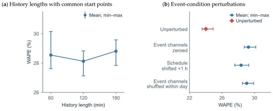
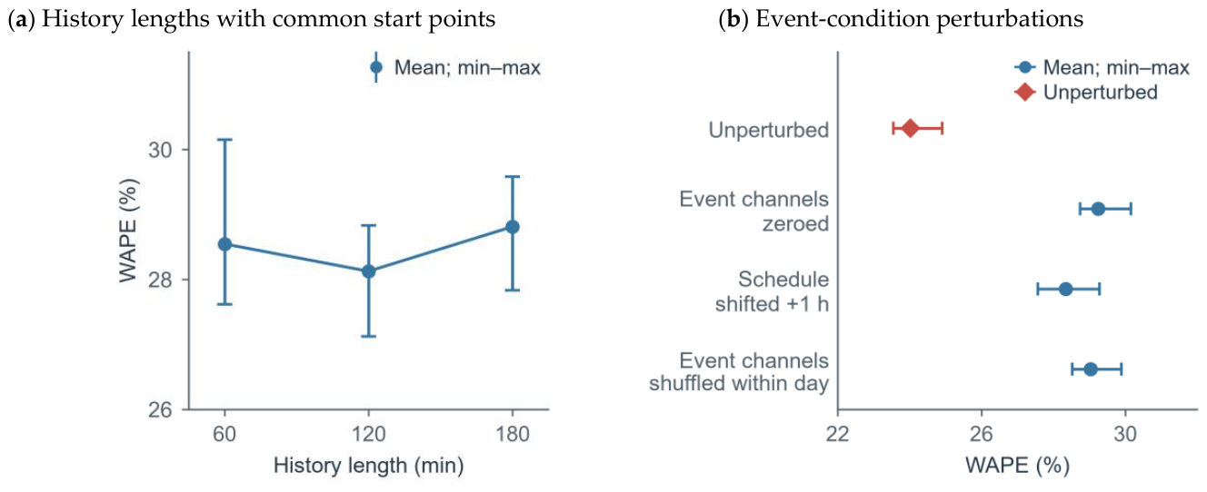
Under the common-sample protocol in Section 3.3, Figure 9a and Table 21 compare models refitted with histories of 4, 8 and 12 steps. Their station-level aggregate WAPE values for the event-window union were 28.55%, 28.12% and 28.81%, respectively. The 8-step configuration achieved a comparatively low mean error in this experiment. The 8-step configuration was refitted using common sample start points, which differ from the sample-start protocol used for the main experiment in Table 2. In Table 21 and Table 22, MAE and RMSE are measured in trips/study-station direction/15 min, and WAPE ranges give the minimum and maximum across three seeds.

Figure 9. Sensitivity to history length and event conditions.

Table 21. History-length sensitivity under common sampling.

Model/Setting	WAPE/%	WAPE Range/%	MAE	RMSE	R2
4-step history	28.55	27.61–30.15	43.23	75.00	0.811
8-step history	28.12	27.12–28.83	42.60	73.19	0.820
12-step history	28.81	27.83–29.58	43.64	74.77	0.812

Table 22. Event-condition perturbations with fixed model weights.

Model/Setting	WAPE/%	WAPE Range/%	MAE	RMSE	R2
Unperturbed	24.02	23.55–24.91	36.38	59.44	0.881
Event channels zeroed	29.24	28.74–30.16	44.29	76.82	0.802
Schedule shifted 1 h later	28.34	27.57–29.28	42.92	73.72	0.817
Event channels shuffled within day	29.03	28.53–29.89	43.97	76.40	0.804

With model weights fixed and passenger-flow history and calendar channels retained, the event channels were separately zeroed, shifted 1 h later or shuffled within each day. Figure 9b and Table 22 show that the WAPE of 24.02% with unperturbed event inputs was 5.22, 4.32 and 5.01 percentage points lower than the 29.24%, 28.34% and 29.03% obtained under these perturbations, respectively. These results support the contribution of event inputs and their temporal alignment to core-station prediction in these experiments.

5. Discussion

5.1. Complementary Information

The structural ablations support the complementary roles of cross-station information and recent OD histories. Disabling the OD-history decoding term produces the largest change in station-aggregate WAPE, indicating that pair-specific histories add predictive information to shared station representations. Fixed graphs encode geographic proximity and travel links observed during training, while OD histories update at each forecast time to capture recent changes. Together, they represent spatial connections and temporal changes in event demand.

Event inputs provide schedules and spatial exposure known in advance, while loss weighting changes the influence of arrival/departure samples on training. In the refitted comparisons in Section 4.3.2, using both produces lower mean aggregate error than using either alone. The fixed-weight perturbations in Section 4.3.3 show that predictions depend on the event conditions and their temporal alignment.

5.2. Practical Value

The unified OD output and its derived margins provide travel allocations and station demand volumes, respectively. Station-aggregate results can be combined with event schedules to identify periods and directions with concentrated demand, while OD results indicate how flows are distributed among origins and destinations. The MAE differences in Table 15 express reductions in mean absolute error in the corresponding trip units, providing a scale reference for using these two types of demand information. Both can serve as demand inputs for passenger guidance, capacity preparation and staff deployment, with their use guided by the respective evaluation granularity and error magnitude.

This study directly evaluates the forecast for the next 15 min. The model also generates steps two to four, corresponding to the following three 15 min intervals. Combined with event schedules, these outputs can serve as candidate information for rolling demand assessment and advance preparation. In the main comparison, station-aggregate WAPE over the arrival/departure-window union is on average 11.28% lower than that of Independent TCN in relative terms; the paired difference and uncertainty over the event-window union are reported in Table 15. Previous research predicts emergency demand on metro sections during disruptions [32]. The present study uses planned-event schedules to provide short-term demand information.

5.3. Research Outlook

The study covers two ordinary days and two event days for the same core-station group. The event-window experiments use historical event observations and recent dates for fitting and calibration. Additional independent events and venues would allow evaluation of first-time events, transfer across months, and applicability to a wider range of ordinary days and periods outside event windows. The three random seeds describe training variability; event-level uncertainty requires more independent event samples.

Comparisons using a common log1p transformation of historical passenger-flow inputs show that the input transformation and corresponding parameter adaptation affect models differently. Table 1 compares representative methods by inputs, relationship modeling and supervision; a common-data benchmark could further evaluate their predictive performance.

The study performs offline forecasting with aggregated OD data. Deployment requires historical OD flows, event schedules available at forecast time, size proxies and station mappings; station histories are derived from the same OD data. Size proxies use venue capacity or other event statistics rather than measured attendance at an individual event. If OD records become available only after journeys are completed or entered into the database, both recent OD histories and their derived margins are affected by the delay. The available 15 min aggregates lack individual journey and database-entry timestamps needed to reconstruct the actual arrival process, so this effect cannot yet be quantified. With model weights fixed, shifting the schedule 1 h later changes station-aggregate WAPE from 24.02% to 28.34% (Table 22), showing the dependence of predictions on schedule alignment. Last-minute rescheduling, event cancellation, mapping errors, station closures and transfer controls may change the conditions and travel links, requiring updated condition information and checks on the applicability of the relationships. When extending the network, shared encoders and low-rank endpoint representations allow the modeling structure to be reused, but dense-graph storage, graph propagation, and OD-history and output computations in the current implementation increase with the numbers of stations and OD pairs. The latency reported in Section 3.1 for the 42-station configuration must be considered separately from data aggregation, transmission and service overheads; end-to-end operation on larger networks requires independent testing.

Local peak amplitudes and response timing can be further improved. On 27 May, the observed destination-flow peak at station A was 813 trips at 16:45, compared with 649.66 trips predicted at that time using seed 2024. At station B, the observed and predicted origin flows at 22:15 were 199 and 89.75 trips, respectively. Both predicted peaks lagged by 15 min. Values at the observed peak time describe amplitude error, whereas the time of the predicted curve maximum describes peak-timing error; the two are evaluated separately. In road-traffic cases, DL-Traff observed lags in LSTNet, DCRNN and Graph WaveNet during sharp fluctuations [33], providing related evidence on responses to abrupt changes. Research on shape and time distortion losses distinguishes and improves shape and temporal-localization errors through the training objective [34]. Incorporating entry-gate control information, journey-time lags and peak-sensitive training objectives could improve local responses, alongside further evaluation of sparse OD pairs and other forecast horizons. Summation guarantees consistency among subnetwork outputs; operational benefits still require validation against line conditions, capacity and decision losses.

6. Conclusions

This study presents DMG-STNet, which combines recent OD histories, shared cross-station information and event conditions for each forecast step, and derives station margins from a single OD output to jointly supervise travel allocations and demand volumes. Evaluation covers 122 OD pairs linked to the core stations on two ordinary days and two event days, with a focus on event and arrival/departure demand for two planned concerts at the same venue.

In the main comparison, DMG-STNet achieves lower daily WAPE, MAE and RMSE for linked OD pairs than the other five models on all four test days. Across the two event days, OD WAPE over the event-window union is 52.94% and station-aggregate WAPE is 24.02%, reflecting predictive accuracy for fine-grained travel allocations and aggregate demand, respectively. In comparisons using a common log1p transformation of historical passenger-flow inputs, DMG-STNet retains lower mean OD and station-aggregate WAPE than the three deep baselines in the event and arrival/departure windows. Structural and event-configuration comparisons provide further results at both evaluation levels.

The unified OD output and its derived margins provide corresponding information on travel allocations and demand volumes for the planned events examined, supporting short-term demand assessment. Future work can further improve OD prediction accuracy and local peak-amplitude and peak-timing responses in station-aggregate forecasts, and evaluate applicability using independent events and different venues.

References

- Xue, G.; Liu, S.; Ren, L.; Ma, Y.; Gong, D. Forecasting the subway passenger flow under event occurrences with multivariate disturbances. Expert Syst. Appl. 2022, 188, 116057. [Google Scholar] [CrossRef] [Scilit]
- Zhang, J.; Che, H.; Chen, F.; Ma, W.; He, Z. Short-term origin-destination demand prediction in urban rail transit systems: A channel-wise attentive split-convolutional neural network method. Transp. Res. Part C Emerg. Technol. 2021, 124, 102928. [Google Scholar] [CrossRef] [Scilit]
- Zhou, W.; Gao, C.; Tang, T. Parallel Interactive Attention Network for Short-Term Origin–Destination Prediction in Urban Rail Transit. Appl. Sci. 2024, 14, 100. [Google Scholar] [CrossRef] [Scilit]
- Huang, H.; Mao, J.; Liu, R.; Lu, W.; Tang, T.; Liu, L. MTLMetro: A Deep Multi-Task Learning Model for Metro Passenger Demands Prediction. IEEE Trans. Intell. Transp. Syst. 2024, 25, 11805–11820. [Google Scholar] [CrossRef] [Scilit]
- Liu, Y.; Chen, B.; Zheng, Y.; Cheng, L.; Li, G.; Lin, L. ODMixer: Fine-Grained Spatial-Temporal MLP for Metro Origin-Destination Prediction. IEEE Trans. Knowl. Data Eng. 2025, 37, 5508–5522. [Google Scholar] [CrossRef] [Scilit]
- Duan, Z.; Gu, M.; Luo, S. A multi-resolution spatiotemporal semantic learning approach for origin-destination demand prediction in urban rail transit network. Comput. Ind. Eng. 2026, 211, 111623. [Google Scholar] [CrossRef] [Scilit]
- Liu, L.; Zhu, Y.; Li, G.; Wu, Z.; Bai, L.; Lin, L. Online Metro Origin-Destination Prediction via Heterogeneous Information Aggregation. IEEE Trans. Pattern Anal. Mach. Intell. 2023, 45, 3574–3589. [Google Scholar] [CrossRef] [Scilit] [PubMed]
- Defferrard, M.; Bresson, X.; Vandergheynst, P. Convolutional Neural Networks on Graphs with Fast Localized Spectral Filtering. In Proceedings of the 30th Conference on Neural Information Processing Systems (NIPS), Barcelona, Spain, 5–10 December 2016; pp. 3844–3852. Available online: https://proceedings.neurips.cc/paper/2016/hash/04df4d434d481c5bb723be1b6df1ee65-Abstract.html (accessed on 20 September 2026).
- Kipf, T.N.; Welling, M. Semi-Supervised Classification with Graph Convolutional Networks. In Proceedings of the 5th International Conference on Learning Representations (ICLR), Toulon, France, 24–26 April 2017. [Google Scholar]
- Liu, L.; Chen, J.; Wu, H.; Zhen, J.; Li, G.; Lin, L. Physical-Virtual Collaboration Modeling for Intra- and Inter-Station Metro Ridership Prediction. IEEE Trans. Intell. Transp. Syst. 2022, 23, 3377–3391. [Google Scholar] [CrossRef] [Scilit]
- Yu, B.; Yin, H.; Zhu, Z. Spatio-Temporal Graph Convolutional Networks: A Deep Learning Framework for Traffic Forecasting. In Proceedings of the Twenty-Seventh International Joint Conference on Artificial Intelligence, Stockholm, Sweden, 13–19 July 2018; pp. 3634–3640. [Google Scholar] [CrossRef] [Scilit] [PubMed]
- Wu, Z.; Pan, S.; Long, G.; Jiang, J.; Zhang, C. Graph WaveNet for Deep Spatial-Temporal Graph Modeling. In Proceedings of the Twenty-Eighth International Joint Conference on Artificial Intelligence, Macao, China, 10–16 August 2019; pp. 1907–1913. [Google Scholar] [CrossRef] [Scilit] [PubMed]
- Li, Y.; Yu, R.; Shahabi, C.; Liu, Y. Diffusion Convolutional Recurrent Neural Network: Data-Driven Traffic Forecasting. In Proceedings of the 6th International Conference on Learning Representations (ICLR), Vancouver, BC, Canada, 30 April–3 May 2018. [Google Scholar]
- Veličković, P.; Cucurull, G.; Casanova, A.; Romero, A.; Liò, P.; Bengio, Y. Graph Attention Networks. In Proceedings of the 6th International Conference on Learning Representations (ICLR), Vancouver, BC, Canada, 30 April–3 May 2018. [Google Scholar]
- Wang, X.; Zhang, Y.; Zhang, J. Large-Scale Origin–Destination Prediction for Urban Rail Transit Network Based on Graph Convolutional Neural Network. Sustainability 2024, 16, 10190. [Google Scholar] [CrossRef] [Scilit]
- Chang, Y.; Zong, M.; Dang, Y.; Wang, K. Multi-Step Passenger Flow Prediction for Urban Metro System Based on Spatial-Temporal Graph Neural Network. Appl. Sci. 2024, 14, 8121. [Google Scholar] [CrossRef] [Scilit]
- Xing, X.; Wang, B.; Ning, X.; Wang, G.; Tiwari, P. Short-term OD flow prediction for urban rail transit control: A multi-graph spatiotemporal fusion approach. Inf. Fusion 2025, 118, 102950. [Google Scholar] [CrossRef] [Scilit]
- Cheng, Z.; Trépanier, M.; Sun, L. Real-Time Forecasting of Metro Origin-Destination Matrices with High-Order Weighted Dynamic Mode Decomposition. Transp. Sci. 2022, 56, 904–918. [Google Scholar] [CrossRef] [Scilit]
- Kim, S.H.; Jeong, H.J.; Shin, S.I.; Kwon, J.W. A Non-Autoregressive Spatiotemporal Framework for Offline Full-Matrix Origin–Destination Forecasting in Large-Scale Metro Networks. Appl. Sci. 2026, 16, 5333. [Google Scholar] [CrossRef] [Scilit]
- Su, A.; Wu, B.; Fang, X. Short-Term Metro Passenger OD Demand Forecasting Based on Low-Rank Tensor Network Extended Kalman Filter. ISPRS Int. J. Geo-Inf. 2026, 15, 327. [Google Scholar] [CrossRef] [Scilit]
- Hou, Z.; Han, J.; Yang, G. Analysis of Passenger Flow Characteristics and Origin–Destination Passenger Flow Prediction in Urban Rail Transit Based on Deep Learning. Appl. Sci. 2025, 15, 2853. [Google Scholar] [CrossRef] [Scilit]
- Fan, Q.; Yu, C.; Zuo, J. Predicting Urban Rail Transit Network Origin–Destination Matrix Under Operational Incidents with Deep Counterfactual Inference. Appl. Sci. 2025, 15, 6398. [Google Scholar] [CrossRef] [Scilit]
- Lim, B.; Arık, S.Ö.; Loeff, N.; Pfister, T. Temporal Fusion Transformers for interpretable multi-horizon time series forecasting. Int. J. Forecast. 2021, 37, 1748–1764. [Google Scholar] [CrossRef] [Scilit]
- Yang, Q.; Xu, X.; Yu, J.; Gao, Q.; Zhang, C. CATI: Cross-Attention-Based Task Interaction for Multi-Granular Metro Passenger Flow Forecasting. Symmetry 2026, 18, 809. [Google Scholar] [CrossRef] [Scilit]
- Wickramasuriya, S.L.; Athanasopoulos, G.; Hyndman, R.J. Optimal Forecast Reconciliation for Hierarchical and Grouped Time Series Through Trace Minimization. J. Am. Stat. Assoc. 2019, 114, 804–819. [Google Scholar] [CrossRef] [Scilit]
- CTS-2024-Dataset. CTS-Transmit GitHub Repository. Available online: https://github.com/Africar-Lee/CTS-transmit/tree/67c4eaef155926ee0e5ab3f735f1caa6b1b5c21c/CTS-2024-dataset (accessed on 21 September 2026).
- Bai, S.; Kolter, J.Z.; Koltun, V. An Empirical Evaluation of Generic Convolutional and Recurrent Networks for Sequence Modeling. arXiv 2018, arXiv:1803.01271. [Google Scholar] [CrossRef] [Scilit]
- Huber, P.J. Robust Estimation of a Location Parameter. Ann. Math. Stat. 1964, 35, 73–101. [Google Scholar] [CrossRef] [Scilit]
- Loshchilov, I.; Hutter, F. Decoupled Weight Decay Regularization. In Proceedings of the 7th International Conference on Learning Representations (ICLR), New Orleans, LA, USA, 6–9 May 2019; Available online: https://openreview.net/forum?id=Bkg6RiCqY7 (accessed on 20 September 2026).
- Xie, P.; Ma, M.; Li, T.; Ji, S.; Du, S.; Yu, Z.; Zhang, J. Spatio-Temporal Dynamic Graph Relation Learning for Urban Metro Flow Prediction. IEEE Trans. Knowl. Data Eng. 2023, 35, 9973–9984. [Google Scholar] [CrossRef] [Scilit]
- Hoerl, A.E.; Kennard, R.W. Ridge Regression: Biased Estimation for Nonorthogonal Problems. Technometrics 1970, 12, 55–67. [Google Scholar] [CrossRef]
- Ma, J.; Zeng, X.; Xue, X.; Deng, R. Metro Emergency Passenger Flow Prediction on Transfer Learning and LSTM Model. Appl. Sci. 2022, 12, 1644. [Google Scholar] [CrossRef] [Scilit]
- Jiang, R.; Yin, D.; Wang, Z.; Wang, Y.; Deng, J.; Liu, H.; Cai, Z.; Deng, J.; Song, X.; Shibasaki, R. DL-Traff: Survey and Benchmark of Deep Learning Models for Urban Traffic Prediction. In Proceedings of the 30th ACM International Conference on Information and Knowledge Management (CIKM ’21), Virtual Event, QLD, Australia, 1–5 November 2021. [Google Scholar] [CrossRef] [Scilit]
- Le Guen, V.; Thome, N. Shape and Time Distortion Loss for Training Deep Time Series Forecasting Models. In Proceedings of the Advances in Neural Information Processing Systems, Vancouver, BC, Canada, 8–14 December 2019; Volume 32. Available online: https://papers.nips.cc/paper_files/paper/2019/hash/466accbac9a66b805ba50e42ad715740-Abstract.html (accessed on 22 October 2026).
Disclaimer/Publisher’s Note: The statements, opinions and data contained in all publications are solely those of the individual author(s) and contributor(s) and not of MDPI and/or the editor(s). MDPI and/or the editor(s) disclaim responsibility for any injury to people or property resulting from any ideas, methods, instructions or products referred to in the content. |
© 2026 by the authors. Licensee MDPI, Basel, Switzerland. This article is an open access article distributed under the terms and conditions of the Creative Commons Attribution (CC BY) license.