Low-Temperature Tensile Strength of J55 and P110 Tubular Steels and an Elastic Consistency Check of a Scaled Tubular Model

Abstract

This study reports the tensile strengths of J55 and P110 tubular steels at low temperatures and assesses the consistency of the geometry, loading, and material inputs in an existing single-tube Abaqus/Explicit model. Ten tensile tests were conducted at five chamber temperatures from −60 to 20 °C, with one specimen per grade–temperature condition. Force and extensometer measurements were recorded at a crosshead speed of 3 mm/min after at least 30 min of thermal conditioning. Between 20 and −60 °C, J55 yield strength increased from 403 to 436 MPa (8.2%) and ultimate tensile strength from 609 to 718 MPa (17.9%). The corresponding P110 values increased from 876 to 952 MPa (8.7%) and from 984 to 1057 MPa (7.4%). For the documented 1000 mm model, a 120 kN axial force gives an analytical nominal stress of approximately 551 MPa and an elastic elongation of 2.71 mm. The model contains a single set of temperature-dependent plasticity inputs obtained by processing experimental curves for both steels. This combined set does not provide separate constitutive descriptions of J55 and P110. Its initial plastic stresses are all above 551 MPa, so the nominal calculation assesses elastic consistency only. The results document the measured strength changes and the scope of the existing model; independent validation is still required for grade-specific plastic deformation and fracture predictions.

1. Introduction

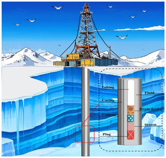
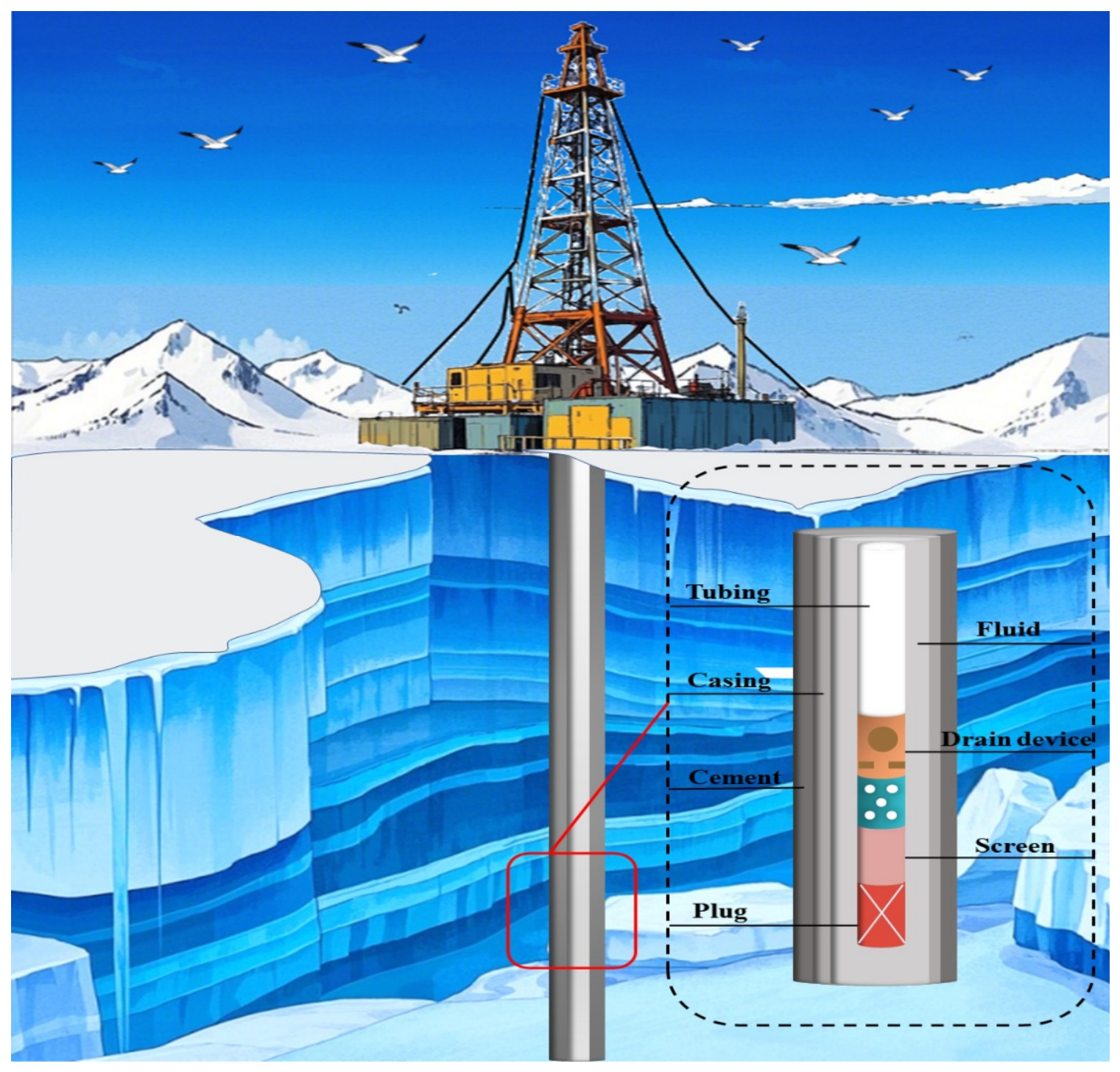
Oil and gas operations in polar and permafrost regions face low temperatures, sea ice, and restricted access to infrastructure. Figure 1 illustrates the tubular-string system and surrounding wellbore environment considered in this study. Loading history and prestrain affect ductile-fracture initiation in steels [1], while operating constraints and dynamic loads influence the response of tubular strings [2]. Low temperatures can also alter material strength, ductility, and failure behavior.

Figure 1. Schematic of a polar tubular-string system and its surrounding wellbore context.

Low-temperature changes in the deformation capacity and impact resistance of tubing and casing steels are relevant to well integrity. Cyclic and impact loads may compound these effects [3]. Characterizing the mechanical response of tubular steels under cold conditions is therefore a necessary part of assessing their suitability for polar operations [4].

Experimental studies have characterized the low-temperature response of several ferrous alloys and structural steels. Straffelini et al. [5] investigated impact deformation and fracture in porous iron and Fe–Ni–Cu–Mo–C alloys using notched and unnotched specimens between room temperature and −60 °C. Plastic bending dominated energy absorption in the unnotched porous-iron specimens, and the absorbed energy decreased with temperature. Menzemer et al. [6] related the reduction in alloy-steel impact toughness to microstructure, local stress state, and macroscopic fracture behavior. Feng et al. [7] used three-point bending to determine critical crack-tip opening displacement and J-integral values, both of which decreased as temperature fell. Tensile tests on Q460C steel also showed increases in yield and ultimate tensile strength at lower temperatures [8,9].

Yan et al. [10] measured stress–strain response, elastic modulus, yield strength, ultimate tensile strength, and fracture strain for normal-strength mild steel and S690 steel at temperatures relevant to Arctic service. Ma et al. [11] tested 66 specimens from cold-formed steel hollow sections with nominal yield stresses of 700, 900, and 1100 MPa and proposed a constitutive description based on the Ramberg–Osgood relation. Using ANSYS, Xu et al. [12] found that initial imperfections and welding residual stresses affected the local-buckling stress of 960 MPa steel columns under compression more strongly than their ultimate resistance.

Tong et al. [13] compared the impact toughness of the base metal, heat-affected zone, and weld metal in four high-strength structural steels. Azhari et al. [14] observed increased strength and reduced ductility in Grade 1200 steel tested at −40 and −80 °C. Niu et al. [15] related the low-temperature toughness and impact crack propagation of X80 pipeline steel to its effective grain size. Chen et al. [16] characterized the tensile response of Q890 and Q960 steels and their weld metals down to −75 °C. Other studies have examined empirical predictions of steel properties at low temperatures [17], Q460C fracture toughness [18], temperature-dependent structural-steel properties [19], and tower-steel impact toughness [20].

When extracting conventional coupons from an operating tubular is impractical, instrumented indentation, full-field measurements, and inverse finite-element analysis can provide complementary estimates of local elastoplastic properties and residual stress [21]. These methods were not used in the present study but offer a possible approach to future local material characterization.

Numerical studies of metallic fracture have used stress-state-dependent ductile-damage models, subzero fracture assessments of tubular joints, descriptions of the ductile-to-brittle transition, temperature- and rate-dependent phase-field models, and structural-scale pipeline simulations [22,23,24,25,26]. These approaches require explicitly defined damage parameters and validation against fracture measurements, beyond agreement in yield and ultimate tensile strength.

For a material model to represent a particular steel grade, the input values must be traceable to that grade’s measurements and processing procedure. Documenting an input file establishes what was assigned to the model; agreement in nominal stress or strength alone does not validate a fracture law.

This study reports the measured yield and ultimate tensile strengths of J55 and P110 and examines the geometry, loading, and material inputs of an existing scaled single-tube model. The existing model contains one temperature-dependent plasticity set obtained by processing the tensile curves of both steels, as documented in Section 2.4. It is a combined model input rather than two separate grade-specific calibrations. The measurements and model settings are therefore reported with their respective scopes: the tests establish the recorded strength differences, while the analytical calculation checks the nominal elastic response implied by the assigned geometry, applied force, and elastic modulus.

The plasticity and damage inputs are documented to explain the configuration and limitations of the existing model. The damage parameters were assigned separately and were not calibrated against the tensile tests. Prescribed temperature selects the corresponding plasticity entries; heat transfer, thermal expansion, and feedback from deformation to temperature are not included.

The available evidence supports a comparison of measured tensile strengths and an analytical check of the model settings. It does not establish physical fracture times, microscopic fracture mechanisms, buckling, service life, or a ranking of the steels by structural fracture resistance.

2. Materials and Methods

2.1. Numerical Formulation and Scope

The analytical assessment calculates nominal axial stress and elastic elongation from the tube geometry, applied force, and isotropic elastic constants. The existing Abaqus model additionally contains temperature-dependent von Mises plasticity with isotropic hardening, ductile-damage initiation, linear displacement-based damage evolution, and element deletion. Section 2.4 documents a combined plasticity input derived from the authors’ tensile curves for J55 and P110. The separately assigned damage inputs have not been calibrated as fracture properties of either grade.

Temperature is prescribed as a uniform field without thermal expansion or heat-transfer calculations. Because the same elastic constants are used at all five model temperatures, the analytical elastic response is independent of temperature. Section 2.2, Section 2.3 and Section 2.4 describe the model settings and material inputs.

2.2. Nominal and Computational Geometry

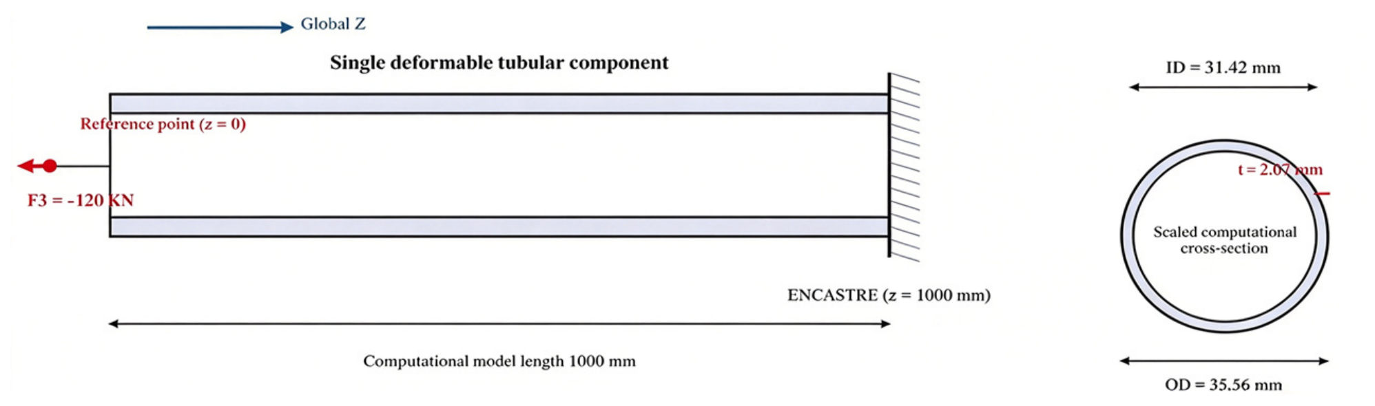
The nominal tube has an outer diameter of 177.80 mm and an inner diameter of 157.10 mm, corresponding to a radial wall thickness of 10.35 mm. In the documented model, the cross-sectional dimensions were scaled by 0.20 and the length was set to 1000 mm. The modeled outer diameter, inner diameter, and wall thickness are approximately 35.56, 31.42, and 2.07 mm, respectively (Table 1). This geometry represents a numerical specimen rather than an API-qualified full-scale component.

Table 1. Nominal tubular dimensions and dimensions of the scaled finite-element model.

Geometry	Length (mm)	OD (mm)	ID (mm)	Radial Thickness (mm)
Nominal tubular dimensions	Not specified	177.80	157.10	10.35
Scaled finite-element model	1000	≈35.56	≈31.42	≈2.07

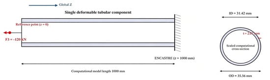
Figure 2 shows the single deformable tube included in the model. The end at z = 1000 mm is fully fixed. The end at z = 0 is coupled to a reference point and loaded in the negative global Z direction to produce axial tension. The casing, screen, connectors, and supports are outside the computational domain, so no contact, tie, or friction interactions are defined.

Figure 2. Geometry, boundary conditions, and axial loading of the scaled single-tube model.

2.3. Model Discretization, Loading, and Temperature Assignment

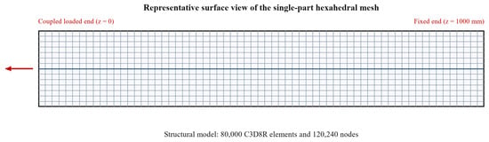
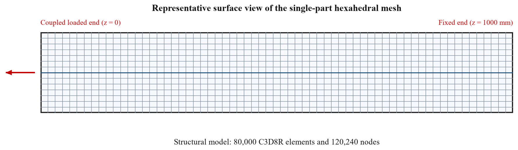
The existing model was created in Abaqus/CAE 2022 for analysis with Abaqus/Explicit. The mesh contains 80,000 eight-node reduced-integration hexahedral elements (C3D8R) and 120,240 nodes (Figure 3). An ENCASTRE boundary condition fixes the end at z = 1000 mm, while the end at z = 0 is kinematically coupled to a reference point. A concentrated axial force increases linearly from 0 to −120 kN over the first second and remains constant until the end of the 23 s step. Geometric nonlinearity is enabled. Fixed mass scaling uses a target time increment of 0.005 s. The default linear and quadratic bulk-viscosity coefficients are 0.06 and 1.2, respectively; these are numerical stabilization settings, without calibration as physical damping. Field output is requested at 200 intervals.

Figure 3. Representative surface view of the scaled tubular mesh (80,000 C3D8R elements and 120,240 nodes).

Five uniform temperature fields (−60, −40, −20, 0, and 20 °C) select the corresponding plasticity inputs. Deformation and dissipation do not update the temperature field, and no thermal expansion coefficient or reference temperature is assigned. The model therefore excludes heat transfer, thermal gradients, and thermal-expansion stresses. The applied force belongs to the scaled numerical specimen. It is not converted to a full-scale load because geometric and dynamic similitude were not imposed.

The corresponding structural-model settings, including the solver, mesh, boundary conditions, loading, step settings, mass scaling, bulk viscosity, interactions, temperature assignment, and field output, are summarized in Table 2.

Table 2. Structural-model settings.

Item	Setting
Software and solver	Abaqus/CAE 2022; Abaqus/Explicit
Geometry	Single tubular part; length 1000 mm; OD ≈ 35.56 mm; ID ≈ 31.42 mm
Discretization	C3D8R; 80,000 elements; 120,240 nodes
Boundary conditions	z = 1000 mm: ENCASTRE; z = 0: kinematic coupling to reference point
Loading	Global direction 3; 0 to −120 kN during 0–1 s; −120 kN during 1–23 s
Step	Explicit dynamic; 23 s; NLGEOM enabled;
Mass scaling	Fixed; target time increment 0.005 s
Bulk viscosity	Linear 0.06; quadratic 1.2 (numerical stabilization)
Interactions	No contact, tie, or friction interaction
Temperature	Uniform prescribed field selecting temperature-indexed plasticity data
Field output	200 intervals

2.4. Low-Temperature Tensile Tests and Material Definition

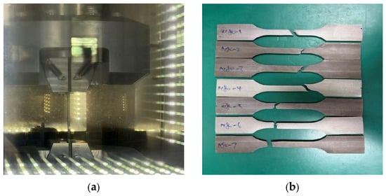
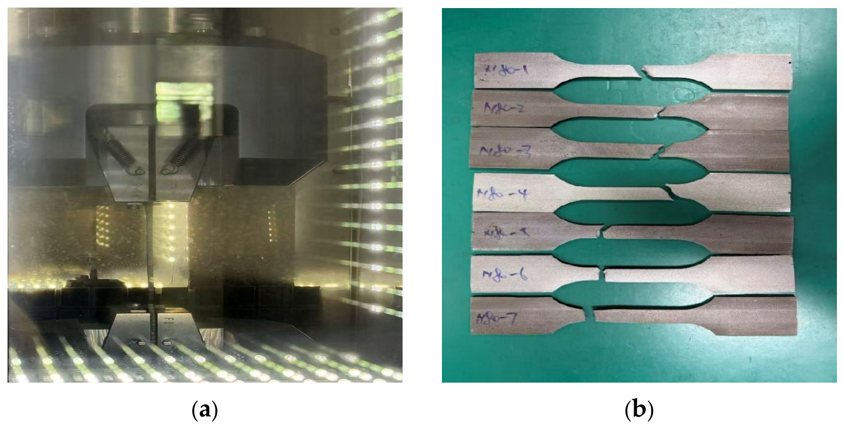
Flat specimens were wire-cut from J55 and P110 tubular products and machined with reference to GB/T 228.3-2019 [27]. Their overall length, reduced parallel length, reduced-section width, thickness, fillet radius, grip width, and grip length were 190, 48, 12.5, 3.0, 25, 35, and 50 mm, respectively. Tests used a 250 kN SUNS UTM5000 machine at a crosshead speed of 3 mm/min. Loading began after the chamber reached its setpoint and the specimens had been held for at least 30 min. The five setpoints were −60, −40, −20, 0 and 20 °C. One specimen was tested for each grade–temperature condition, giving 10 tests. Force and axial strain were acquired in real time using the force sensor and extensometer; crosshead displacement was also recorded. Figure 4 shows the equipment and representative specimens, and Table 3 summarizes the test conditions.

Figure 4. Equipment and specimens for the low-temperature tensile tests. (a) Universal testing machine. (b) Low-temperature tensile specimen.

Table 3. Low-temperature tensile test conditions.

Experimental Item	Setting
Standard	Specimen preparation and tensile testing with reference to GB/T 228.3-2019
Reported grades	J55 and P110
Specimen	190 mm overall; 48 mm parallel; 12.5 mm width; 3.0 mm thickness; R25 mm
Machine	SUNS UTM5000; 250 kN capacity
Crosshead speed	3 mm/min (nominal crosshead-based rate ≈ 1.04 × 10−3 s−1)
Temperatures	−60, −40, −20, 0, and 20 °C
Conditioning	At least 30 min at the chamber setpoint
Replication	n = 1 per grade–temperature condition; 10 tests
Recorded channels	Force, extensometer strain, and crosshead displacement
Yield-strength determination	Automatic calculation by MaterialTest 5.4 software (SUNS UTM5000) from force and extensometer measurements using a routine appropriate to the recorded yielding behavior

The reported temperatures refer to the chamber setpoints, as a separate continuous record of specimen temperature is unavailable. Dividing the crosshead speed by the 48 mm parallel length gives a nominal strain-rate estimate of 1.04 × 10⁻³ s⁻¹. This estimate characterizes the loading protocol and is distinct from the strain measured by the extensometer and the local equivalent plastic strain rate used in the damage model.

The SUNS UTM5000 universal testing machine (Shenzhen SUNS Technology Stock Co., Ltd., Shenzhen, China) acquired force and extensometer measurements in real time, and its manufacturer-supplied software generated the stress–strain curves and calculated yield-related properties according to the observed yielding behavior. For curves with a distinct yield stage, the evaluation identifies the upper yield strength (ReH), the maximum stress before the first force decrease, and the lower yield strength (ReL), the minimum stress during yielding after excluding initial transient effects. For curves without a distinct yield stage, the 0.2% proof strength (Rp0.2) is determined from the intersection of the stress–strain curve with a line parallel to the elastic segment and offset by 0.002 strain. The reported yield strengths are the test-system outputs. These alternative criteria explain the evaluation procedure; they do not identify which output label applies to each reported value, so the values are not retrospectively relabeled as ReH, ReL, or Rp0.2.

Table 4 summarizes the material definition used in the finite-element model, including the assigned elastic constants, the combined temperature-dependent plasticity input, and the separately assigned damage parameters. Table 5 presents the single temperature-dependent plasticity dataset used in the model at −60, −40, −20, 0, and 20 °C. This dataset was obtained by processing the authors’ experimental stress–strain curves for J55 and P110 and converting the resulting values into stress–equivalent-plastic-strain format. The tensile tests are the experimental source, and Table 5 reports the values assigned to the model. Each temperature has one sequence of four stress values rather than a separate sequence for each grade. The available processing record does not specify how the data from the two steels were combined; therefore, a specific averaging, weighting, or fitting procedure cannot be reported reproducibly.

Table 4. Assigned elastic properties, combined plasticity input, and damage parameters.

Input	Value or Option
Density	7.8 × 10−9 tonne/mm3
Elasticity	E = 203,000 MPa; ν = 0.30
Plasticity	One temperature-dependent set constructed from J55 and P110 tensile curves (Table 5); grade-specific calibration is not established
Damage initiation	One archived row: initiation strain 0.10; triaxiality 0.3333; equivalent plastic strain-rate coordinate 1.0 s−1. Not calibrated to the tests.
Damage evolution	Archived linear displacement-based softening; equivalent plastic displacement 0.10 mm; no independent calibration
Temperature dependency	Temperature-dependent plasticity; temperature-independent damage initiation and evolution
Thermal formulation	No heat transfer, thermal expansion, or deformation-to-temperature feedback
Toughness inputs	No Charpy, KIC, JIC, CTOD, or independently measured fracture-energy input

Table 5. Temperature-dependent plasticity dataset used in the finite-element model.

Temperature (°C)	εp = 0	εp = 0.025	εp = 0.072	εp = 0.182
−60	917	923	928	931
−40	690	696	701	709
−20	670	674	682	687
0	650	657	663	670
20	627	634	639	647

The assigned elastic modulus, Poisson’s ratio, and density are E = 203,000 MPa, ν = 0.30, and 7.8 × 10⁻⁹ tonne/mm³, respectively. Table 5 lists the plasticity inputs at −60, −40, −20, 0, and 20 °C. The experimental strain records were obtained using an extensometer. These measurements describe axial strain over its gauge length but do not independently resolve local true strain after necking. Additional measurements and an appropriate conversion procedure are needed for post-necking constitutive and fracture calibration.

The ductile-damage initiation table contains one entry: an equivalent plastic strain at initiation of 0.10, a stress triaxiality of 0.3333, and an equivalent plastic strain rate of 1.0 s⁻¹. The third value is the rate coordinate associated with the tabulated initiation strain, rather than an applied loading rate, time increment, or dimensionless factor [28]. A single rate entry does not establish calibrated rate dependence. The damage inputs are independent of temperature.

The nominal experimental rate, (3/60)/48 ≈ 1.04 × 10⁻³ s⁻¹, is approximately 960 times lower than the damage-table rate of 1.0 s⁻¹. These quantities have different meanings: the former is estimated from crosshead motion, while the latter is a local equivalent plastic strain-rate coordinate. The existing record does not establish rate matching or justify the selected damage-table value. Replacing it with the nominal experimental rate would require damage calibration and a new analysis.

Damage evolution uses linear displacement-based softening with an equivalent plastic displacement of 0.10 mm, followed by element deletion [28]. The initiation and evolution inputs have not been independently calibrated against fracture strain, force–displacement response, dissipated energy, or multiaxial fracture data. Charpy energy and fracture-mechanics quantities such as CTOD and the J-integral are not model inputs. The ideal uniform elastic calculation does not activate or assess these damage parameters.

Together, Table 4 and Table 5 document the assigned model inputs rather than independently validated grade-specific constitutive and fracture properties. Validation of the plasticity and fracture response requires additional grade-specific measurements and calibration.

The dataset was obtained by processing the tensile-test curves of J55 and P110. Values are stress inputs in MPa at the stated equivalent plastic strains; they are not separate constitutive data for each grade.

The combined input in Table 5 must be distinguished from the grade-specific measurements in Table 6. At 20 °C, its initial plastic stress is 627 MPa, whereas the recorded yield strengths are 403 MPa for J55 and 876 MPa for P110. At −60 °C, the corresponding values are 917, 436, and 952 MPa. These differences preclude identifying the Table 5 values as the measured yield strengths of both steels. The combined set is retained to document the existing model, but it cannot establish the plastic or fracture response of either grade. Reproducible material calibration requires the original curve identifiers, their grade and temperature assignments, and the actual conversion and combination procedure. Moreover, comparison against the same data used to construct an input set is a calibration check, not independent validation.

Table 6. Measured yield and ultimate tensile strengths of J55 and P110 steels at the five test temperatures; one specimen was tested for each grade–temperature condition.

Steel	Temperature (°C)	Yield Strength (MPa)	Ultimate Tensile Strength (MPa)
J55	−60	436	718
J55	−40	430	711
J55	−20	419	652
J55	0	415	649
J55	20	403	609
P110	−60	952	1057
P110	−40	925	1039
P110	−20	885	992
P110	0	880	987
P110	20	876	984

3. Results and Discussion

3.1. Low-Temperature Tensile-Strength Observations

Table 6 presents the recorded yield and ultimate tensile strengths for all five test temperatures. The values are approximate and rounded to the nearest MPa. For J55, the yield strength decreased from approximately 436 MPa at −60 °C to 430, 419, 415, and 403 MPa at −40, −20, 0, and 20 °C, respectively. Over the same temperature sequence, the ultimate tensile strength decreased from approximately 718 to 711, 652, 649, and 609 MPa.

For P110, the yield strength decreased from approximately 952 MPa at −60 °C to 925, 885, 880, and 876 MPa at −40, −20, 0, and 20 °C, respectively. The ultimate tensile strength decreased from approximately 1057 to 1039, 992, 987, and 984 MPa. Thus, both steels exhibited higher recorded strengths at lower temperatures across the five tested conditions. Between 20 and −60 °C, J55 exhibited increases of 8.2% in yield strength and 17.9% in ultimate tensile strength, whereas the corresponding increases for P110 were 8.7% and 7.4%.

These values are individual specimen observations. They document the complete five-temperature test matrix but do not quantify scatter, confidence intervals, or statistically significant differences between grades. The yield strengths were calculated by the test system from force and extensometer measurements. Strength values alone do not determine fracture strain, fracture energy, or fracture toughness.

3.2. Analytical Check of the Structural Model

The modeled cross-sectional area, A = π(OD² − ID²)/4, is approximately 217.8 mm². An axial force of 120,000 N therefore gives a nominal stress F/A of approximately 551 MPa. With E = 203,000 MPa and L = 1000 mm, the corresponding elastic elongation FL/(AE) is approximately 2.71 mm. These analytical values describe a uniformly loaded elastic tube and check the consistency of the specified geometry, force, and modulus. They are not results extracted from the finite-element solution.

The initial plastic stresses in Table 5 range from 627 MPa at 20 °C to 917 MPa at −60 °C. Each exceeds the nominal stress of 551 MPa, so the uniform axial calculation remains below plastic initiation for this particular material card. The plasticity and damage entries therefore do not affect the analytical result. The nominal stress and elastic elongation are identical at all five temperatures because geometry, load, and elastic modulus are unchanged.

This conclusion applies to the assigned material card and cannot be transferred directly to either tested steel. In particular, 551 MPa exceeds the recorded J55 yield strengths of 403 and 436 MPa at 20 and −60 °C. The present check therefore does not establish elastic behavior for a J55 tube under the same nominal stress. It also cannot show that every integration point in an Explicit simulation remains elastic: end constraints and transient effects require examination of finite-element fields and energy histories. No conclusion about quasi-static equivalence, physical fracture timing, acceleration oscillations, or the relative structural fracture resistance of J55 and P110 is drawn from this calculation.

3.3. Study Limitations

One specimen was tested per grade–temperature condition, so repeatability and statistical scatter were not assessed. The extensometer measurements support the reported stress–strain response but do not resolve local post-necking strain. Table 5 originates from processing the authors’ tensile curves, although its point-by-point construction from the two grades is not documented sufficiently for independent reproduction. It therefore remains a combined model input without a demonstrated grade-specific calibration. The damage parameters also lack calibration at the experimental loading rate. The numerical assessment is limited to an analytical check; energy-balance, loading-rate, time-step, and mesh-convergence studies have not been supplied. Agreement in nominal stress or tensile strength cannot resolve these limitations.

4. Conclusions

Cooling from 20 to −60 °C increased the recorded yield and ultimate tensile strengths of both tested steels. For J55, the values increased from 403 to 436 MPa (8.2%) and from 609 to 718 MPa (17.9%), respectively. For P110, they increased from 876 to 952 MPa (8.7%) and from 984 to 1057 MPa (7.4%). J55 showed the larger relative change in ultimate tensile strength, while P110 retained the higher absolute strength. These findings describe the tested specimens; replicated measurements are needed to quantify variability.

For the documented 1000 mm model with a cross-sectional area of approximately 217.8 mm², a 120 kN force gives a nominal stress of 551 MPa and an elastic elongation of 2.71 mm. This stress is below the initial plastic stresses of 627–917 MPa in the assigned material card. The analytical result therefore checks elastic consistency for that input set. It does not validate plasticity or damage and cannot be interpreted as evidence that J55 remains elastic at the same nominal stress.

The study brings together measured strength changes and an explicit check of the mechanical conditions represented by an existing tubular model. It identifies a necessary distinction between the separate J55/P110 measurements and the single plasticity set constructed from both steels. Comparing the applied nominal stress with the model’s initial plastic stress makes the scope of the calculation clear. Establishing grade-specific constitutive behavior additionally requires a reproducible account of how the experimental curves were processed.

For engineering assessment, the measured strengths provide specimen-level information about the response to cooling. Increased tensile strength alone does not establish improved fracture resistance. Material selection should also consider ductility, toughness, defects, and service loading. The present combined material input does not support a structural ranking of J55 and P110; such comparisons require independently calibrated constitutive and fracture descriptions for each grade.

Further work should document the complete processing of each grade’s tensile curves and include replicated tests, full force–displacement records, and fracture measurements. Notched or other multiaxial tests would support damage calibration over relevant temperatures and strain rates. Numerical verification should examine energy balance, loading rate, mass scaling, time-step sensitivity, and mesh dependence before component-scale validation. These steps are needed to extend the current assessment to quantitative predictions of low-temperature tubular fracture.

References

- Enami, K. The effects of compressive and tensile prestrain on ductile fracture initiation in steels. Eng. Fract. Mech. 2005, 72, 1089–1105. [Google Scholar] [CrossRef] [Scilit]
- Deng, Q.; Jiang, J.; Yang, D.; Han, H.; Qi, G. Dynamic analysis and optimization of perforated tubing strings in deep-water wells under diverse operating conditions. Ocean Eng. 2025, 322, 120535. [Google Scholar] [CrossRef] [Scilit]
- Yan, J.B.; Luo, Y.L.; Su, L.; Lin, X.; Luo, Y.B.; Zhang, L. Low-temperature compression behaviour of square CFST columns using Q960 ultra-high strength steel. J. Constr. Steel Res. 2021, 183, 106727. [Google Scholar] [CrossRef] [Scilit]
- Ren, X.; Nordhagen, H.O.; Zhang, Z.; Akselsen, O.M. Tensile properties of 420 MPa steel at low temperature. In Proceedings of the ISOPE International Ocean and Polar Engineering Conference, Big Island, HI, USA, 21–26 June 2015. [Google Scholar]
- Straffelini, G.; Fontanari, V.; Molinari, A. Impact fracture toughness of porous alloys between room temperature and −60 °C. Mater. Sci. Eng. A 1999, 272, 389–397. [Google Scholar] [CrossRef] [Scilit]
- Menzemer, C.C.; Srivatsan, T.S.; Ortiz, R.; Al-Hajri, M.; Petraroli, M. Influence of temperature on impact fracture behavior of an alloy steel. Mater. Des. 2001, 22, 659–667. [Google Scholar] [CrossRef] [Scilit]
- Feng, B.; Wang, Y.; Shi, Y. Analysis of Fracture Surface and Elastoplastic Fracture Toughness of Railway Rail Steel at Low Temperature. Low Temp. Archit. Technol. 2007, 3, 4. [Google Scholar]
- Wang, Y.; Zhang, H.; Gao, D.; Ke, K.; Liu, W. Mechanical Properties Test and Strength Design of Drill String Materials in Low-Temperature Environments. Pet. Drill. Tech. 2021, 49, 35–41. [Google Scholar]
- Wang, Y.; Lin, Y.; Zhang, Y.; Shi, Y. Low Temperature Fracture Toughness Test of High Strength Steel Q460C. J. Jilin Univ. (Eng. Technol. Ed.) 2012, 42, 6. [Google Scholar] [CrossRef]
- Yan, J.B.; Liew, J.R.; Zhang, M.H.; Wang, J.Y. Mechanical properties of normal strength mild steel and high strength steel S690 in low temperature relevant to Arctic environment. Mater. Des. 2014, 61, 150–159. [Google Scholar] [CrossRef] [Scilit]
- Ma, J.L.; Chan, T.M.; Young, B. Material properties and residual stresses of cold-formed high strength steel hollow sections. J. Constr. Steel Res. 2015, 109, 152–165. [Google Scholar] [CrossRef] [Scilit]
- Xu, K.; Shi, G.; Lin, C. Analysis and design method on local buckling behavior of 960 MPa high strength steel columns under axial compression. Nat. Sci. 2017, 44, 102–111. [Google Scholar]
- Tong, L.; Niu, L.; Jing, S.; Ai, L.; Zhao, X.L. Low temperature impact toughness of high strength structural steel. Thin-Walled Struct. 2018, 132, 410–420. [Google Scholar] [CrossRef] [Scilit]
- Azhari, F.; Apon, A.A.H.; Heidarpour, A.; Zhao, X.L.; Hutchinson, C.R. Mechanical response of ultra-high strength (Grade 1200) steel under extreme cooling conditions. Constr. Build. Mater. 2018, 175, 790–803. [Google Scholar] [CrossRef] [Scilit]
- Niu, Y.; Liu, Q.; Jia, S.; Wang, B.; Ren, Y. Microstructure and Impact Toughness of X80 High Strength Low Alloy Pipeline Steel. Iron Steel 2019, 2, 9. [Google Scholar] [CrossRef]
- Chen, M.T.; Cai, A.; Pandey, M.; Shen, C.; Zhang, Y.; Hu, L. Mechanical properties of high strength steels and weld metals at arctic low temperatures. Thin-Walled Struct. 2023, 185, 110543. [Google Scholar] [CrossRef] [Scilit]
- Wang, Y. Grey Prediction Method for Variation Rule of Mechanical Properties of Steel at Low Temperature. J. Shenyang Jianzhu Univ. (Nat. Sci.) 2014, 30, 9. [Google Scholar]
- Wang, Y.Q.; Lin, Y.; Zhang, Y.N.; Shi, Y.J. Experimental study on fracture toughness of Q460C the high-strength construction steel at low temperature. Appl. Mech. Mater. 2011, 71, 890–897. [Google Scholar] [CrossRef] [Scilit]
- Wang, Y.; Wu, Y.; Shi, Y.; Wang, X.; Zhang, Y. Experimental Study on the Effect of Low Temperature on the Main Mechanical Properties of Structural Steel. J. Railw. Sci. Eng. 2005, 2, 4. [Google Scholar] [CrossRef]
- Wang, Y.; Liao, X.; Zhang, Z.; Liu, X.; Xing, H. Experiment on Mechanical Properties and Impact Toughness of Steel for Transmission Tower at Low Temperature. J. Harbin Inst. Technol. 2015, 47, 5. [Google Scholar]
- Buljak, V.; Cocchetti, G.; Cornaggia, A.; Maier, G. Assessment of residual stresses and mechanical characterization of materials by ‘hole drilling’ and indentation tests combined and by inverse analysis. Mech. Res. Commun. 2015, 68, 18–24. [Google Scholar] [CrossRef] [Scilit]
- Jia, L.J.; Kuwamura, H. Ductile fracture simulation of structural steels under monotonic tension. J. Struct. Eng. 2014, 140, 04013115. [Google Scholar] [CrossRef] [Scilit]
- Björk, T.; Heinilä, S.; Marquis, G. Assessment of subzero fracture of welded tubular K-joint. J. Struct. Eng. 2008, 134, 181–188. [Google Scholar] [CrossRef] [Scilit]
- Nam, W.; Hopperstad, O.S.; Amdahl, J. Modelling of the ductile-brittle fracture transition in steel structures with large shell elements: A numerical study. Mar. Struct. 2018, 62, 40–59. [Google Scholar] [CrossRef] [Scilit]
- Marandi, S.M.; Nourbakhsh, S.H.; Botshekanan Dehkordi, M.; Badnava, H. Finite element implementation of coupled temperature-rate dependent fracture using the phase field model. Mech. Mater. 2020, 148, 103449. [Google Scholar] [CrossRef] [Scilit]
- Talemi, R.; Cooreman, S.; Mahgerefteh, H.; Martynov, S.; Brown, S. A fully coupled fluid-structure interaction simulation of three-dimensional dynamic ductile fracture in a steel pipeline. Theor. Appl. Fract. Mech. 2019, 101, 224–235. [Google Scholar] [CrossRef] [Scilit]
- GB/T 228.3-2019; Metallic Materials—Tensile Testing—Part 3: Method of Test at Low Temperature. Standardization Administration of China: Beijing, China, 2019.
- Dassault Systèmes SIMULIA. Abaqus 2022 Documentation: Material Data Definition; Damage for Ductile Metals; Damage Evolution and Element Removal; Abaqus/Explicit Analysis; Dassault Systèmes: Providence, RI, USA, 2022. [Google Scholar]
Disclaimer/Publisher’s Note: The statements, opinions and data contained in all publications are solely those of the individual author(s) and contributor(s) and not of MDPI and/or the editor(s). MDPI and/or the editor(s) disclaim responsibility for any injury to people or property resulting from any ideas, methods, instructions or products referred to in the content. |
© 2026 by the authors. Licensee MDPI, Basel, Switzerland. This article is an open access article distributed under the terms and conditions of the Creative Commons Attribution (CC BY) license.