Numerical Evaluation of a Mirror-Slope Rockfill Replacement for Embankments in Warm Island Permafrost

Featured Application

The proposed mirror-slope rockfill layer (MSRL) can be applied to the design and rehabilitation of highway embankments in warm island permafrost regions. It improves thermal stability and stress transfer near the slope toes, thereby mitigating permafrost degradation and long-term differential deformation and providing guidance for the design of the rockfill replacement extent and slope ratio.

Abstract

Highway embankments in warm island permafrost regions of Northeast China are vulnerable to climate warming and foundation softening. To improve long-term temperature and deformation control, a mirror-slope rockfill layer (MSRL) and corresponding mirror-slope rockfill embankment (MSRE) are proposed by mirroring the embankment side-slope geometry. A two-dimensional hydro–thermal–mechanical model was established for the K49 section of S201 Highway, and 40-year simulations were conducted at a warming rate of 0.06 °C/a for an unprotected embankment, a rectangular rockfill embankment, and four replacement-interface slopes. In Year 40, centerline settlement decreased from 29.20 cm in the unprotected embankment to 0.86 cm in the MSRE. Relative to the rectangular scheme, absolute vertical and horizontal displacements at the right slope toe decreased by 2.10 and 2.90 cm, respectively. Among vertical, 1:1.5, 1:2.5, and 1:3.5 interfaces, the 1:2.5 MSRL reduced maximum shear stress and rockfill consumption by 30.1% and 16.4%, respectively, relative to the vertical interface. Further flattening to 1:3.5 provided limited mechanical improvement but increased slope-toe temperature fluctuations. The 1:2.5 MSRL therefore offers a feasible balance among thermal control, deformation control, and material consumption under the investigated conditions.

1. Introduction

With ongoing warming [1,2], permafrost in Northeast China has undergone continuous degradation [3,4,5]. Permafrost thaw reduces the stability of ice-rich subgrades and increases the risks of thaw settlement and differential embankment deformation [6,7]. Long-term deformation control of subgrades in warm island permafrost is therefore of considerable engineering importance.

Rockfill replacement is a direct method for treating permafrost foundations. Previous studies have focused mainly on replacement material and thickness. Researchers have compared the effects of rockfill, breccia, and gravel on foundation temperature and deformation [8] and investigated ground-temperature variations for different rockfill replacement thicknesses [9]. These studies indicate that rockfill replacement can improve the thermal stability of the underlying permafrost and reduce embankment deformation caused by permafrost degradation [8,9].

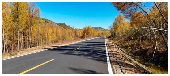
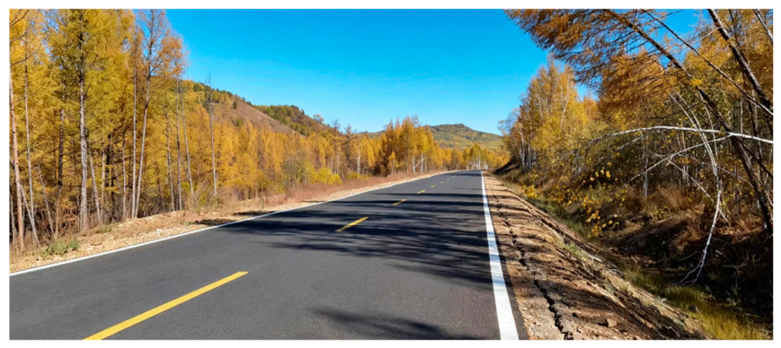
Layer geometry affects both the replacement extent and rockfill consumption and may also alter the temperature and stress distributions within the subgrade. Conventional replacement layers are commonly rectangular, with vertical side boundaries at which stress concentrations can develop. Under asymmetric heating of the two side slopes, the likelihood of slope cracking may increase (Figure 1). Accordingly, this study proposes a mirror-slope rockfill layer (MSRL) based on the mirrored geometry of the embankment-fill cross-section. The two inclined sides of the MSRL follow the embankment slope ratio of 1:2.5 and extend toward both slope toes. The study examines whether this geometry can reduce stress concentrations and improve the temperature and deformation fields near the embankment.

Figure 1. Longitudinal cracks on the side slope of a rectangular rockfill replacement road section.

In addition to replacement materials and thickness, previous studies have also proposed geometric schemes such as base rockfill layers, slope rockfill revetments, slope rockfill interlayers, composite structures for sunny–shady slopes, and L-shaped rockfill embankments [10,11,12,13,14]. Most of these schemes rely on exposed or ventilated rockfill layers to enhance heat dissipation. In contrast, the MSRL proposed in this paper adopts excavation and replacement, burying the rockfill layer into the soft clay foundation. It simultaneously compares temperature, deformation, stress, and material consumption per linear meter. Therefore, this paper focuses on the mirror-slope interface design under buried replacement conditions and its multi-criteria evaluation.

Because field tests are constrained by differences in climate, stratigraphy, and construction conditions, as well as by the required observation period, this study primarily uses numerical simulation. Model reliability is evaluated using laboratory freezing tests, borehole ground-temperature measurements beneath the natural ground surface, and monitored centerline deformation.

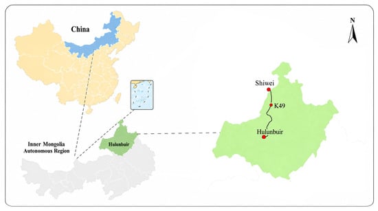
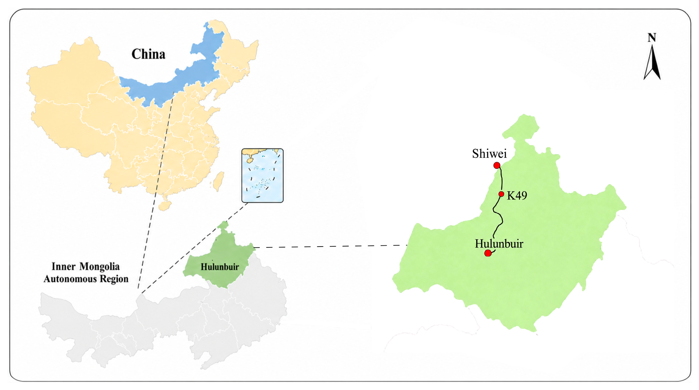
The K49 cross-section of S201 Highway (Figure 2) is investigated using a two-dimensional hydro–thermal–mechanical model. Three questions are addressed: first, whether the mirror-slope replacement scheme can slow the downward migration of the centerline thermal interface and reduce calculated settlement relative to an unprotected embankment; second, how the slope-toe temperature, displacement, and stress differ between the complete mirror-slope and rectangular schemes at the same design thickness; and third, how the mechanical response, temperature fluctuations, and material consumption of four candidate interface slopes can be balanced for a prescribed top width and maximum replacement depth. The results provide a reference for the geometric design of rockfill replacement layers in warm island permafrost regions.

Figure 2. Location of the study area Blue indicates the Inner Mongolia Autonomous Region, and green indicates Hulunbuir. Red dots mark Shiwei, the K49 study section, and Hulunbuir; the black line shows the S201 Highway alignment, and the dashed lines indicate the corresponding enlarged map extents.

2. Materials and Methods

A simplified two-dimensional hydro–thermal–mechanical model was developed from the governing equations for unsaturated seepage, heat transfer with phase change, and plane-strain mechanics. Each material domain was treated as homogeneous and isotropic, with parameters assigned separately to the different domains.

2.1. Governing Equations for the Temperature Field with Phase Change in Frozen Soil

Unsaturated frozen soil consists of soil particles, unfrozen water, ice, and gas. Heat transfer in each material domain was described using an equivalent-continuum approach [15,16]. Only the latent heat of the ice–water phase change was considered; vapor migration, convective heat carried by liquid-water migration, and airflow within rockfill pores were neglected. The governing equation is:

$${\rho C}_{eff}{\displaystyle \frac{\mathsf{\partial }T}{\mathsf{\partial }t}}=\mathsf{\nabla }\cdot \left({\lambda }_{eff}\mathsf{\nabla }T\right)+{\rho }_i{\displaystyle \frac{\mathsf{\partial }{\theta }_i}{\mathsf{\partial }t}}L,$$

(1)

$$C_{eff}=\{\begin{array}{cc}{C}_f& T<T_f-∆T\\ C_f+{\displaystyle \frac{C_u-C_f}{2∆T}}\left[T-\left(T_f-∆T\right)\right]& T_f-∆T\le T\le T_f+∆T\\ C_u& T>T_f+∆T\end{array},$$

(2)

$${\lambda }_{eff}=\{\begin{array}{cc}{\lambda }_f& T<T_f-∆T\\ {\lambda }_f+{\displaystyle \frac{{\lambda }_u-{\lambda }_f}{2∆T}}[T-\left(T_f-∆T\right)]& T_f-∆T\le T\le T_f+∆T,\\ {\lambda }_u& T>T_f+∆T\end{array}$$

(3)

where $\rho$ is the soil density (kg·m⁻³); θ is the volumetric water content; C_eff is the effective mass-specific heat capacity of soil (J·kg⁻¹·°C⁻¹); λ_eff is the effective thermal conductivity of soil (W·m⁻¹·°C⁻¹); $∆T$ = 0.5 °C; $T_f$ = 0 °C; t is time; T is temperature (°C); ∇ is the differential operator; L is the latent heat of the ice–water phase change, L = 335 × 10³ J·kg⁻¹; ${\rho }_i$ is the density of ice (kg·m⁻³); and θ_i is the volumetric ice content of the pores (m³·m⁻³).

2.2. Moisture Migration Equation

With the X-axis positive to the right and the Y-axis positive upward, liquid-water migration was described using Richards’ equation with an ice–water phase-change source/sink term [16,17]. Matric suction and gravity govern liquid-water flux, while temperature affects water migration through the unfrozen-water content and ice-impedance relationship [8,16]. The water-retention curve and relative hydraulic conductivity were represented by van Genuchten-type relationships [18,19], as follows:

$${\displaystyle \frac{\mathsf{\partial }{\theta }_u}{\mathsf{\partial }t}}+{\displaystyle \frac{{\rho }_i}{{\rho }_w}}{\displaystyle \frac{\mathsf{\partial }{\theta }_i}{\mathsf{\partial }t}}=\nabla ·\left[D\left({\theta }_u\right){\nabla \theta }_u\right]+{\displaystyle \frac{\mathsf{\partial }{k}_g\left({\theta }_u\right)}{\mathsf{\partial }y}},$$

(4)

$${\theta }_t={\theta }_u+{\displaystyle \frac{{\rho }_i}{{\rho }_w}}{\theta }_i,$$

(5)

$${{\theta }_t\left(x,y,t\right)|}_{t=0}={\theta }_0\left(x,y,0\right),$$

(6)

$$D({\theta }_u)=\{\begin{array}{cc}{\displaystyle \frac{k_{sat}·k\left({\theta }_u\right)}{c\left({\theta }_u\right)}}& T>T_f\\ {\displaystyle \frac{k_{sat}·k\left({\theta }_u\right)}{c\left({\theta }_u\right)}}{I}_i& T\le T_f\end{array},$$

(7)

$$I_i=10^{-10{\theta }_I},$$

(8)

$${\theta }_u\left({\theta }_t,\mathrm{T}\right)=\{\begin{array}{cc}{\theta }_t& \mathrm{T}\ge {\mathrm{T}}_{\mathrm{f}}\\ \min \left[{\theta }_t,\max \left({\theta }_r,\mathrm{A}{\left|\mathrm{T}\right|}^{\mathrm{B}}\right)\right]& \mathrm{T}<{\mathrm{T}}_{\mathrm{f}}\end{array},$$

(9)

$$S={\displaystyle \frac{{\theta }_u-{\theta }_r}{{\theta }_{sat}-{\theta }_r}},$$

(10)

$$k({\theta }_u)=S^l{[1-{(1-S^{{\displaystyle \frac{1}{m}}})}^m]}^2,$$

(11)

$$c\left({\theta }_u\right)=\alpha \cdot {\displaystyle \frac{m}{\left(1-m\right)}}\cdot \left({\theta }_{sat}-{\theta }_r\right)S^{{\displaystyle \frac{1}{m}}}{(1-S^{{\displaystyle \frac{1}{m}}})}^m,$$

(12)

$$k_g({\theta }_u)=\{\begin{array}{cc}{k}_{sat}\cdot k\left({\theta }_u\right)& T>T_f\\ I_i\cdot k_{sat}\cdot k\left({\theta }_u\right)& T\le T_f\end{array},$$

(13)

where ${\theta }_u$ is the volumetric unfrozen-water content, and A and B are experimental parameters obtained using the temperature-measurement method; θ_t is the total volumetric water content, whose value at t = 0 is the initial value; θ₀ is the initial volumetric water content; T_f is the phase-change temperature (0 °C); ${\rho }_w$ and ${\rho }_i$ are the densities of water and ice, respectively; ${\mathrm{k}}_{\mathrm{g}}\left({\theta }_u\right)$ is the hydraulic conductivity in the gravitational direction; $\mathrm{D}\left({\theta }_u\right)$ is the unfrozen-water diffusivity; $\mathrm{k}\left({\theta }_u\right)$ is the hydraulic conductivity of unsaturated soil; α, m, and l are van Genuchten model parameters; ${\mathrm{I}}_i$ is the impedance factor representing the obstruction of water flow by ice in the pores; θ_sat and θ_r are the saturated and residual volumetric water contents (m³·m⁻³), respectively; S is the effective saturation (0 < S ≤ 1); $\mathrm{c}\left({\theta }_u\right)$ is the specific moisture capacity, i.e., the volume of water released per unit volume of soil for a unit decrease in pressure head (m⁻¹); k is the dimensionless relative hydraulic conductivity; and k_sat is the saturated hydraulic conductivity (m/s).

2.3. Constitutive Relations and Hydro–Thermal–Mechanical Coupling

2.3.1. Constitutive Equations

A two-dimensional plane-strain model was used to analyze the long-term deformation of the embankment and its foundation. Taking the $z$-direction as the longitudinal direction of the road, the plane-strain condition is:

$${\epsilon }_z={\gamma }_{xz}={\gamma }_{yz}=0,$$

(14)

A zero longitudinal strain ${\epsilon }_z$ does not imply zero longitudinal stress. The longitudinal effective stress ${\sigma }_z^{\prime }$ is determined automatically by the constitutive relation and is included in the subsequent stress-invariant and yield-state calculations.

The effective-stress increment of the soil skeleton is:

$$d{\sigma }^{\prime }=D\left(T\right):\left(d\epsilon -d{\epsilon }^p\right),$$

(15)

where ${\sigma }^{\prime }$ is the three-dimensional effective-stress tensor, and $D\left(T\right)$ is the elastic-stiffness tensor defined by the temperature-dependent elastic modulus $E\left(T\right)$ and Poisson’s ratio $\nu$; where $D\left(T\right)$ is the temperature-dependent elastic-stiffness matrix. Under two-dimensional plane-strain conditions and using engineering shear strain, the matrix is:

$$\begin{array}{cccc}& D\left(T\right)={\displaystyle \frac{E\left(T\right)}{\left(1+\nu \right)\left(1-2\nu \right)}}\left[\begin{array}{ccc}1-\nu & \nu & 0\\ \nu & 1-\nu & 0\\ 0& 0& {\displaystyle \frac{1-2\nu }{2}}\end{array}\right],& & \end{array}$$

(16)

where $E\left(T\right)$ is the temperature-dependent elastic modulus and $\nu$ is Poisson’s ratio.

The Drucker–Prager yield function was evaluated using the effective stress of the soil skeleton [20]:

$$F=\sqrt{J_2^{\prime }}+{\alpha }_{\mathrm{D}\mathrm{P}}{I}_1^{\prime }-k\le 0,$$

(17)

The first invariant of the effective-stress tensor, $I_1^{\prime }$, is the sum of the effective normal stresses in the three directions:

$$I_1^{\prime }=\mathrm{tr}\left({\sigma }^{\prime }\right)={\sigma }_x^{\prime }+{\sigma }_y^{\prime }+{\sigma }_z^{\prime },$$

(18)

Under two-dimensional plane-strain conditions, ${\tau }_{xz}^{\prime }={\tau }_{yz}^{\prime }=0$; therefore, the second invariant of the effective deviatoric-stress tensor, $J_2^{\prime }$, is:

$$J_2^{\prime }={\displaystyle \frac{1}{6}}\left[{\left({\sigma }_x^{\prime }-{\sigma }_y^{\prime }\right)}^2+{\left({\sigma }_y^{\prime }-{\sigma }_z^{\prime }\right)}^2+{\left({\sigma }_z^{\prime }-{\sigma }_x^{\prime }\right)}^2\right]+{\left({\tau }_{xy}^{\prime }\right)}^2,$$

(19)

Accordingly, the Drucker–Prager yield function under plane-strain conditions can be fully expanded as:

$$\begin{gathered} F=\sqrt{{\displaystyle \frac{1}{6}}\left[{\left({\sigma }_x^{\prime }-{\sigma }_y^{\prime }\right)}^2+{\left({\sigma }_y^{\prime }-{\sigma }_z^{\prime }\right)}^2+{\left({\sigma }_z^{\prime }-{\sigma }_x^{\prime }\right)}^2\right]+{\left({\tau }_{xy}^{\prime }\right)}^2} \\ +{\alpha }_{\mathrm{D}\mathrm{P}}\left({\sigma }_x^{\prime }+{\sigma }_y^{\prime }+{\sigma }_z^{\prime }\right)-k\le 0, \end{gathered}$$

(20)

where $I_1^{\prime }$ represents the mean pressure level of the effective-stress state and $J_2^{\prime }$ represents the magnitude of the effective deviatoric stress or shear action. The embankment fill, clay, and tuff were modeled using Drucker–Prager elastoplasticity, whereas the rockfill layer was modeled as linear elastic. The plastic-strain increment was calculated using an associated flow rule: This study adopts an associated flow rule, in which the plastic potential function G is identical to the yield function F, and no independent dilation angle is specified. When matching Mohr–Coulomb parameters, this can be interpreted as the dilation angle ψ(T) being equal to the internal friction angle ϕ(T). This setting is applied to the embankment fill, clay, and tuff; the rockfill layer is treated as a linear elastic material and does not involve the plastic flow rule [21,22].

$$\mathrm{d}{\epsilon }^p=\mathrm{d}\lambda {\displaystyle \frac{\mathsf{\partial }F}{\mathsf{\partial }{\sigma }^{\prime }}},\mathrm{d}\lambda \ge 0,$$

(21)

where $\mathrm{d}\lambda$ is the plastic multiplier. When $F<0$, the material remains elastic and $\mathrm{d}\lambda =0$; when the stress reaches the yield surface $F=0$, plastic strain may develop.

Using compression-meridian matching between the Drucker–Prager and Mohr–Coulomb yield surface [23], the parameters ${\alpha }_{\mathrm{D}\mathrm{P}}$ and $k_{DP}$ are determined as:

$${\alpha }_{\mathrm{D}\mathrm{P}}\left(T\right)={\displaystyle \frac{2\sin {\phi }_T}{\sqrt{3}\left(3-\sin {\phi }_T\right)}},$$

(22)

$$k_{\mathrm{D}\mathrm{P}}\left(T\right)={\displaystyle \frac{2\sqrt{3}{c}_T\cos {\phi }_T}{3-\sin {\phi }_T}},$$

(23)

where ${\phi }_T$ and $c_T$ are the internal friction angle and cohesion of the material at temperature $T$, respectively; ${\alpha }_{\mathrm{D}\mathrm{P}}$ is a dimensionless parameter representing pressure sensitivity; and $k_{DP}$ is a strength parameter controlling the size of the yield surface and has units of stress.

2.3.2. Hydro–Thermal–Mechanical Coupling Relationships

The mechanical analysis primarily considered two coupling mechanisms: pore-water effective stress and temperature-dependent strength. The former represents changes in pore-water pressure and matric suction caused by precipitation infiltration, evaporation, and moisture migration; the latter represents the effects of pore-ice bonding and thaw-induced softening on soil stiffness and strength.

Because volumetric unfrozen-water content was used as the state variable in the moisture-migration equation, the matric pressure head was obtained by inverting the van Genuchten water-retention relationship:

$$h_m=-{\displaystyle \frac{1}{\alpha }}{\left(S^{-{\displaystyle \frac{1}{m}}}-1\right)}^{{\displaystyle \frac{1}{n}}},n={\displaystyle \frac{1}{1-m}},$$

(24)

The pore-water pressure is:

$$p_w={\rho }_{w}g{h}_m,$$

(25)

The pore-air pressure was taken as zero gauge pressure, i.e., $p_a=0$. To account for the effects of pore-water pressure and matric suction on the soil-skeleton stress under unsaturated conditions, the Bishop equivalent pore pressure was introduced [24,25]:

$$p_B=\{\begin{array}{cc}{p}_w,& p_w\ge p_a,\\ p_a-\chi \mathrm{m}\mathrm{i}\mathrm{n}(p_a-p_w,s_{max})& p_w<p_a,\end{array},\chi =S^{\beta },$$

(26)

where $\chi$ is the Bishop effective-stress parameter, with $\beta =1.0$ adopted in this study; $s_{\mathrm{m}\mathrm{a}\mathrm{x}}$ is the suction cap used in the mechanical calculation to prevent unrealistically high suction as the material approaches its residual water content. A value of $s_{\mathrm{m}\mathrm{a}\mathrm{x}}=100$ kPa was used for the embankment fill, clay, and tuff, and 20 kPa was used for the more freely draining rockfill layer.

Taking tensile stress as positive, the relationship between total stress and the effective stress of the soil skeleton is [26]:

$$\sigma ={\sigma }^{\prime }-b_{\mathrm{B}}{p}_B·I,$$

(27)

$$\mathrm{I}=\left\{\begin{array}{ccc}1& 0& 0\\ 0& 1& 0\\ 0& 0& 1\end{array}\right\},$$

(28)

The corresponding quasi-static equilibrium equation is:

$$\nabla \cdot \left({\sigma }^{\prime }-b_{\mathrm{B}}{p}_B·\mathrm{I}\right)+\rho g=0,$$

(29)

where $b_{\mathrm{B}}$ is the Biot coefficient, taken as 1.0 for the embankment fill, clay, and rockfill layer and 0.8 for the tuff. In this simplified model, pore ice was treated as part of the soil skeleton and ice pressure was not calculated separately. Ice-bonding enhancement and thaw-induced softening were represented through experimentally fitted, temperature-dependent elastic modulus, cohesion, and internal friction angle.

2.4. Geometric Models and Simulation Cases

2.4.1. MSRE and Unprotected Embankment

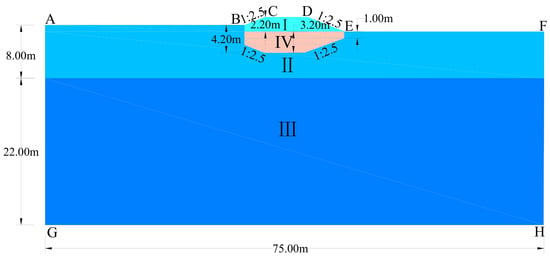
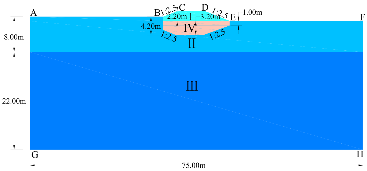
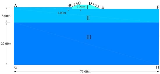
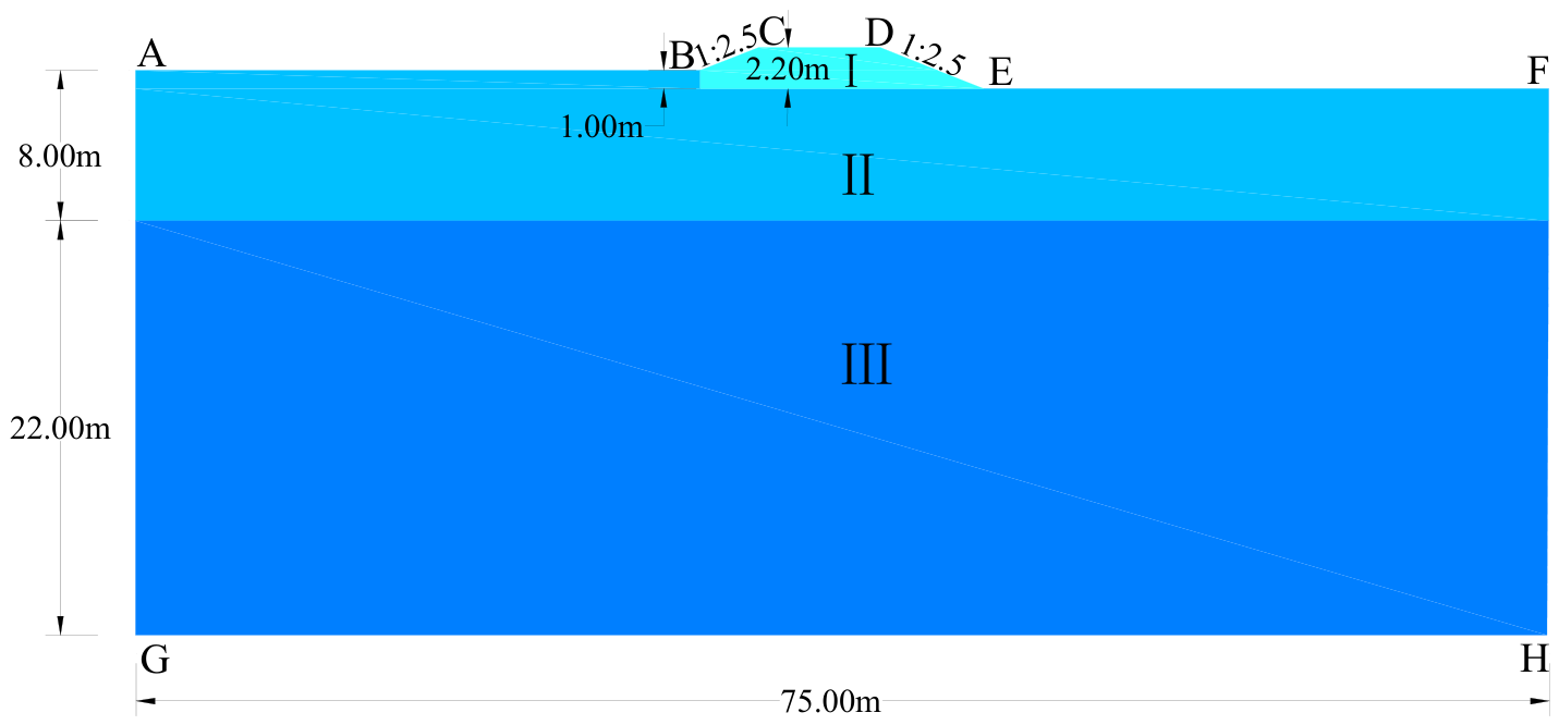
Models of the MSRE and the unprotected embankment were established from the engineering design of the K49 cross-section of S201 Highway (Figure 3 and Figure 4). The lateral model boundaries extended 30 m outward from each slope toe. From top to bottom, the stratigraphy comprised 2.2 m of embankment fill, 8.00 m of clay, and 22.00 m of tuff. A 3.2 m-thick MSRL was placed within the MSRE foundation. The rockfill consisted of granite particles 10–30 cm in size, with a mean particle size of 18.6 cm.

Figure 3. MSRE model. Points A–H denote the model boundaries; Roman numerals I–IV denote the embankment fill, clay, tuff, and rockfill, respectively. Arrows indicate geometric dimensions and slope ratios, and colors distinguish the material domains.

Figure 4. Unprotected embankment model. Points A–H denote the model boundaries; Roman numerals I–III denote the embankment fill, clay, and tuff, respectively. Arrows indicate geometric dimensions and slope ratios, and colors distinguish the material domains.

The MSRL comprises a mirrored portion and an additional rectangular portion, whose dimensions are governed jointly by the original embankment cross-section and the design replacement thickness (Figure 5). With the base of the embankment fill as the reference, the 2.2 m-high fill cross-section with a side-slope ratio of 1:2.5 was mirrored downward into the foundation, yielding a 2.2 m-thick mirrored portion. A rectangular rockfill layer 15 m long and 1.0 m thick was placed above it. The resulting design structural thickness of the MSRL is:

$$H_{\mathrm{M}\mathrm{S}\mathrm{R}\mathrm{L}}=2.2+1.00=3.2\mathrm{m}.$$

(30)

Figure 5. Geometric configuration of the MSRL. Roman numerals I and II denote the mirrored and rectangular portions of the MSRL, respectively, and III denotes their combined geometry. Arrows indicate geometric dimensions and slope ratios.

Because the natural ground surface is higher on the left than on the right, the top of the rockfill layer is approximately 1.0 m below ground level when referenced to the left-side ground elevation. The maximum construction depth on the left side is therefore:

$$D_{\mathrm{m}\mathrm{a}\mathrm{x}}=1.00+3.2=4.2\mathrm{m}.$$

(31)

The additional rectangular rockfill layer primarily ensures continuity of the replacement layer and construction feasibility. If only the 2.2 m-thick mirrored portion were used, its edge thickness would decrease rapidly along the inclined surface, hindering formation of a continuous coarse-particle skeleton and complicating control of layered placement and compaction.

2.4.2. MSRE and Rectangular Rockfill Embankment

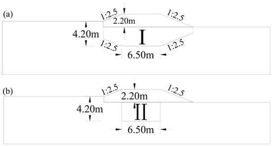
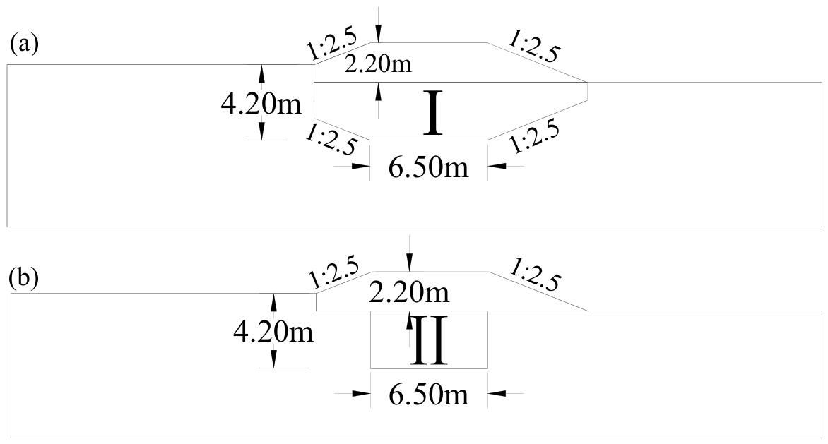
A rectangular rockfill replacement scheme was established as a control under identical material parameters, loads, climatic boundaries, and design thickness (Figure 6) [8,9]. The rectangular rockfill layer was 6.5 m long and 3.2 m thick, with the same particle size as the MSRL. Because this scheme differs from the MSRL in lateral coverage and material consumption, the comparison concerns two complete design schemes rather than geometry alone.

Figure 6. Geometric configurations of the embankment cross-sections: (a) MSRE; (b) conventional rectangular rockfill embankment. Roman numerals I and II denote the rockfill replacement domains in the two schemes, respectively. Arrows indicate geometric dimensions and slope ratios, and colors distinguish the rockfill layers from the surrounding foundation.

2.4.3. Rockfill Embankments with Different Replacement-Interface Slopes

In this study, the replacement-interface slope refers specifically to the inclined contact surface between the rockfill layer and the clay on each side. It is expressed as vertical height: horizontal distance; a larger second term denotes a flatter interface. Previous field observations have shown that transverse temperature asymmetry is closely related to differential deformation of highway embankments in warm permafrost regions [27].

The 1:2.5 interface was initially derived from the mirrored geometry of the original embankment slope. However, this geometric relationship only identifies 1:2.5 as an engineering-based candidate and cannot, by itself, establish it as the most reasonable slope. With the replacement-layer top width, maximum replacement depth, material parameters, and boundary conditions held constant, four candidate schemes—a vertical interface and slopes of 1:1.5, 1:2.5, and 1:3.5 (Figure 7)—were compared in terms of shear stress and slope-toe temperature response. The vertical-interface scheme in this comparison is 15 m wide and differs from the 6.5 m-wide rectangular control scheme described in Section 2.4.2.

Figure 7. Rockfill-layer configurations with different replacement-interface slopes: (a) vertical interface; (b) 1:1.5; (c) 1:2.5 (MSRL); (d) 1:3.5. The cross-sectional areas of the rockfill replacement layer under the four schemes are 48.00, 43.29, 40.15, and 37.01 m², respectively, corresponding to rockfill consumption per linear meter of embankment of 48.00, 43.29, 40.15, and 37.01 m³/m. Roman numerals I–IV denote the vertical, 1:1.5, 1:2.5, and 1:3.5 interface schemes, respectively, and arrows indicate geometric dimensions and slope ratios.

2.5. Boundary Conditions

2.5.1. Temperature Boundary Conditions

The geometric-model boundaries include the natural ground surface, the left and right side-slope surfaces, and the asphalt pavement surface. Temperature boundary conditions were fitted to the measured temperatures at the corresponding locations. The periodic temperature boundaries were fitted using a sinusoidal function, consistent with commonly adopted boundary formulations for permafrost embankments [28,29]. Each temperature boundary was expressed as a sinusoidal function of time:

$$T=T_0+A_0\cdot \sin \left(2\pi t_a+{\alpha }_0\right)+T_1\cdot t_a,$$

(32)

where $T_0$ is the annual mean ground temperature at each boundary; ${\alpha }_0$ is the initial phase angle associated with the construction date. Construction began on 15 July; therefore, ${\alpha }_0$ was set to 0.5π. $t_a$ is time in years; $T_1$ is the local warming rate due to climate change; and $A_0$ is the mean temperature amplitude. To represent an accelerated warming scenario, $T_1$ was set to 0.06 °C/a, which lies between the ensemble warming rates projected for Northern Hemisphere permafrost regions [30].

The remaining temperature-boundary parameters are listed in Table 1.

Table 1. Temperature-boundary parameters.

Boundary	Annual Mean Temperature T0 (°C)	Mean Temperature Amplitude A0 (°C)
Natural ground surface (AB, EF)	−0.54	13.32
Left side slope (BC)	1.05	13.74
Right side slope (DE)	1.09	15.83
Asphalt pavement (CD)	1.13	16.32

The values of $T_0$ and $A_0$ were obtained by least-squares fitting of the temperature records collected at K49 from 2010 to 2020. The phase parameter ${\alpha }_0=0.5\pi$ was determined from the recorded construction start date of 15 July. In this study, the upper thermal boundary was fitted using measured near-surface temperatures at the K49 section from 2010 to 2020, consistent with the approach adopted in previous rockfill replacement studies on the same road section [9]. Therefore, the combined effects of snow cover, solar radiation, and surface heat exchange during the fitting period have been partially incorporated into the boundary parameters [28,31]; however, the model does not explicitly represent snow depth, density, duration, or their interannual variability.

The left and right lateral boundaries were thermally insulated, and a geothermal heat flux of 0.09 W/m², determined from borehole measurements, was applied at the bottom boundary.

Before the formal simulation, a preliminary calculation was performed using periodic temperature boundaries without the linear warming term. The temperature field on 15 July was extracted as the initial field for the long-term simulation.

2.5.2. Moisture Boundary Conditions

The asphalt pavement (CD) and the left and right lateral boundaries (AG and FH) were assigned no-flux moisture boundaries. A total volumetric water content of ${\theta }_t=0.15$, corresponding to the measured initial volumetric water content of the deep tuff layer listed in Table 2 was prescribed at the bottom boundary (GH) to approximate stable deep-stratum moisture conditions. The natural ground surface (AB and EF) and the embankment side slopes (BC and DE) were permeable boundaries, where surface moisture exchange included both precipitation infiltration and evaporation [32].

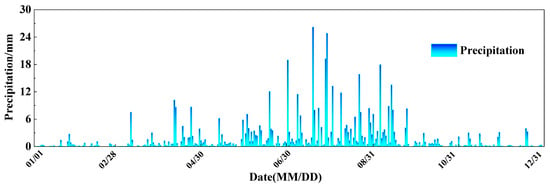
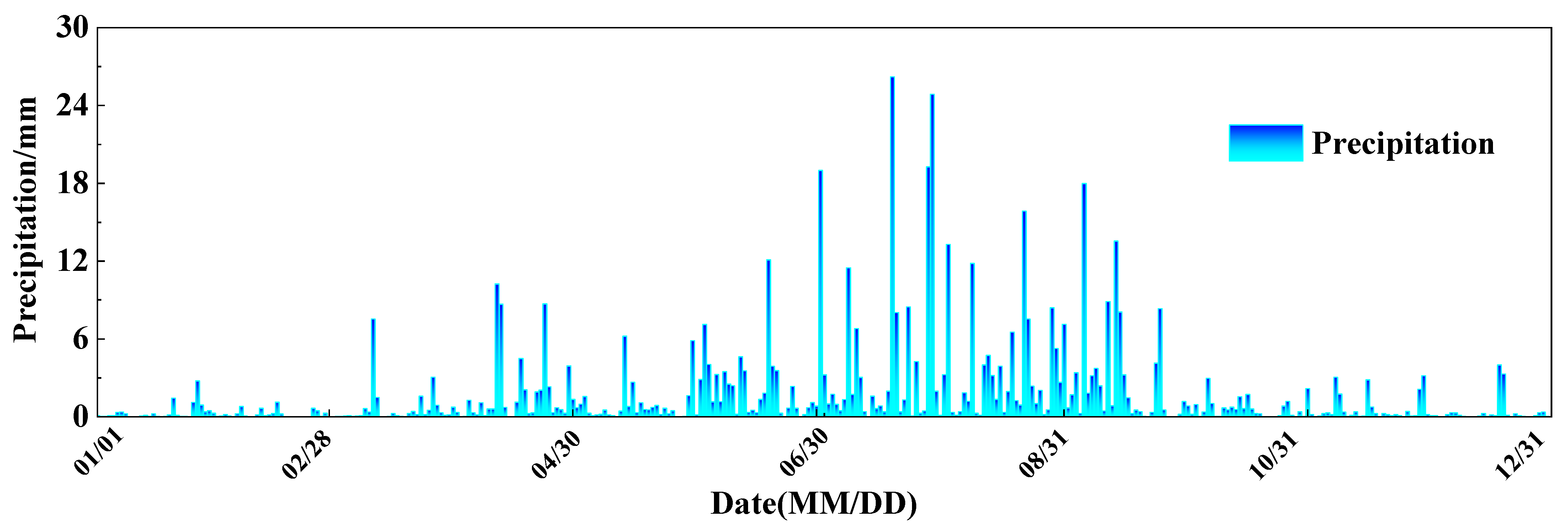
The precipitation boundary was prescribed using daily precipitation data recorded at Hailar National Reference Climatological Station (Station ID: 50527) from 1 January to 31 December 2025 (Figure 8). For days with precipitation, the daily total was distributed uniformly over 24 h and converted to the boundary moisture flux $q_p\left(t\right)$:

$$q_p\left(t\right)={\displaystyle \frac{P_{2025}\left(d\right)}{1000\times 86400}}{H}_p\left(T_a\right),$$

(33)

where $P_{2025}\left(d\right)$ is the daily precipitation on day $d$ (mm); $1000$ and $\mathrm{86,400}$ convert millimeters to meters and days to seconds, respectively; and $H_p\left(T_a\right)$ is an indicator function for liquid precipitation, equal to 1 when the air temperature exceeds 0 °C and 0 otherwise. The threshold of 0 °C was adopted as a simplified binary criterion for rainfall infiltration; actual rain–snow temperature thresholds vary spatially and are affected by humidity and atmospheric pressure [33]. The precipitation flux was set to zero on days without precipitation. For the long-term simulation, the 2025 daily precipitation series was repeated annually to eliminate the effects of interannual precipitation variability.

Figure 8. Daily precipitation in Hulunbuir in 2025.

Because vegetation is sparse in the study area, plant transpiration was neglected, and the outward liquid-water flux caused by surface evaporation was expressed as:

$$q_e=q_{0}SH\left(\mathrm{T}\right),$$

(34)

Because continuous surface-evaporation observations were unavailable for the study area, a simplified empirical evaporation-flux boundary with $q_0=1.0\times {10}^{-8}$ m/s was adopted. This value corresponds to approximately 315 mm/a and was selected as a regional upper-bound reference, close to the mean annual evapotranspiration of approximately 310 mm/a reported for Hulunbuir [34]. Here, $S$ is the effective liquid-water saturation, and $H\left(T\right)$ controls evaporation under frozen conditions:

$$H\left(T\right)=\{\begin{array}{cc}1,& \mathrm{T}>0°\mathrm{C}\\ 0,& \mathrm{T}\le 0°\mathrm{C}\end{array},$$

(35)

where T is the temperature in degrees Celsius. Liquid-water evaporation was considered when the surface temperature exceeded 0 °C and was assumed to cease when the surface temperature was at or below 0 °C. Snow sublimation and plant transpiration were not considered; therefore, this boundary condition is a simplification of actual surface moisture exchange.

2.5.3. Displacement Boundary Conditions and Gravity Loading

The bottom boundary (GH) was fully fixed, whereas roller constraints were applied to the left and right lateral boundaries (AG and FH), leaving vertical displacement unconstrained. The asphalt pavement (CD), natural ground surface (AB and EF), and embankment side slopes (BC and DE) were free boundaries. Continuous connections were assigned among the embankment fill, clay, tuff, and rockfill, assuming continuity of displacement and normal stress across each interface and neglecting interface slip, opening, and separation. The assumption of continuous connection is a first-order simplification in macroscopic continuum models, intended for comparing the freeze–thaw response within each material zone and the overall deformation [8]. It does not imply that the actual rockfill–clay interface is incapable of slipping or opening. Furthermore, the present model does not resolve the detachment, migration, deposition, and clogging processes of fine particles.

Gravity body forces were applied to all material domains included in the solid-mechanics analysis: embankment fill (I), clay (II), tuff (III), and rockfill (IV). The body force in each material domain is:

$$b_i={\rho }_{i}g=\left[\begin{array}{c}0\\ -{\rho }_{i}g\end{array}\right],$$

(36)

where ${\rho }_i$ is the equivalent bulk density of material $i$, $g=9.81\mathrm{m}/{\mathrm{s}}^2$ is gravitational acceleration, and $b_i$ has units of $\mathrm{N}/{\mathrm{m}}^3$. The same form of gravity body force was applied to each comparison case according to its material distribution. Gravity equilibrium was established before the transient calculation; displacements were then reset to zero, and the equilibrated initial stress field was used as the initial condition.

2.5.4. Model Parameters

The parameters for the moisture field were determined from field measurements, laboratory tests, and published sources, as summarized below:

Table 2. Moisture-field parameters of the embankment fill, rockfill, clay, and tuff.

Parameter	A	B	θsat	α (m−1)	m	l	θr	Ksat (m/s)	θ0
Embankment fill	0.08	−0.096	0.23	2.60	0.25	0.5	0.06	1.2 × 10−6	0.14
Rockfill	0.065	−0.210	0.16	20.00	0.75	0.5	0.01	5.0 × 10−2	0.05
Clay	0.12	−0.180	0.40	0.80	0.10	0.5	0.07	1.1 × 10−8	0.24
Tuff	0.11	−0.320	0.24	0.11	0.67	0.5	0.03	1.0 × 10−7	0.15

Note: Values of A, B, θ_sat, θ_r, θ₀, and K_sat were obtained from laboratory tests. The values of α and m were selected with reference to published parameter ranges and material-specific water-retention studies for textural soils, rockfill, and tuff [35,36,37], whereas the pore-connectivity parameter l was set to 0.5 following the Mualem–Van Genuchten formulation [18,19].

Table 2. Moisture-field parameters of the embankment fill, rockfill, clay, and tuff.

Parameter	A	B	θsat	α (m−1)	m	l	θr	Ksat (m/s)	θ0
Embankment fill	0.08	−0.096	0.23	2.60	0.25	0.5	0.06	1.2 × 10−6	0.14
Rockfill	0.065	−0.210	0.16	20.00	0.75	0.5	0.01	5.0 × 10−2	0.05
Clay	0.12	−0.180	0.40	0.80	0.10	0.5	0.07	1.1 × 10−8	0.24
Tuff	0.11	−0.320	0.24	0.11	0.67	0.5	0.03	1.0 × 10−7	0.15

Note: Values of A, B, θ_sat, θ_r, θ₀, and K_sat were obtained from laboratory tests. The values of α and m were selected with reference to published parameter ranges and material-specific water-retention studies for textural soils, rockfill, and tuff [35,36,37], whereas the pore-connectivity parameter l was set to 0.5 following the Mualem–Van Genuchten formulation [18,19].

Based on laboratory-test fitting, the mechanical parameters and physical parameters of the embankment fill, rockfill, clay, and tuff are listed in Table 3 and the corresponding physical parameters are listed in Table 4. Under frozen conditions, the elastic modulus $E_S$ (MPa), internal friction angle $\phi$ (rad), and cohesion $c$ (MPa) of each porous medium are functions of temperature $T$ (°C), as follows:

$$E\left(T\right)=\{\begin{array}{cc}{a}_1+b_1\left|T\right|& T<T_f\\ a_1& T\ge T_f\end{array},$$

(37)

$$\phi \left(T\right)=\{\begin{array}{cc}{a}_2+b_2{\left|T\right|}^{C_2}& T<T_f\\ a_2& T\ge T_f\end{array},$$

(38)

$$c\left(T\right)=\{\begin{array}{cc}{a}_3+b_3{\left|T\right|}^{C_3}& T<T_f\\ a_3& T\ge T_f\end{array},$$

(39)

Table 3. Mechanical parameters of the embankment fill, rockfill, clay, and tuff.

Material	a1	b1	a2	b2	C2	a3	b3	C3	v
Embankment fill	28.0	26.4	0.262	0.017	0.8	0.022	0.41	0.9	0.35
Rockfill	86.0	15.0	N/A	N/A	N/A	N/A	N/A	N/A	0.20
Clay	3.2	2.8	0.202	0.017	1.3	0.068	0.83	0.6	0.40
Tuff	26.0	0.8	0.235	0.011	1.2	0.046	0.13	0.5	0.30

Table 4. Physical parameters of the embankment fill, rockfill, clay, and tuff.

Material	λu (W/m·K)	λf (W/m·K)	Cf (J/kg·K)	Cu (J/kg·K)	ρ (kg/m3)
Embankment fill	1.32	1.68	1543	2297	1937
Rockfill	0.85	1.39	983	1180	2127
Clay	0.70	2.20	1241	1874	1610
Tuff	0.60	2.50	1826	2014	1482

The numerical calculations were performed in COMSOL Multiphysics 5.4. The two-dimensional model used free triangular elements and quadratic Lagrange interpolation. The maximum and minimum element sizes were 2.80 and 0.13 m, respectively. No additional manual local refinement zones were specified; COMSOL automatically generated a graded mesh according to the geometric boundaries and domain sizes, with a denser mesh near the embankment, slope surfaces, and material boundaries, and a coarser mesh in the foundation region away from the embankment. The original mesh contained a total of 940 triangular elements.

For the transient calculation, a first- to second-order implicit backward differentiation formula (BDF) and free time stepping were adopted. The initial and maximum internal time steps were automatically adjusted by the solver based on the error; results were output every 1/12 year. The hydro–thermal–mechanical equations were solved in a fully coupled manner. Nonlinear convergence was determined by a solution-based tolerance criterion with a tolerance factor of 1. The maximum number of nonlinear iterations per time step was 4, and the linear system was solved using a direct solver.

2.6. Model Validation

2.6.1. Laboratory-Test Validation

Laboratory tests were used as the primary validation benchmark. The test conditions were reproduced numerically, and the simulated results were compared with laboratory measurements to evaluate whether the model captured the relevant physical processes [8,16].

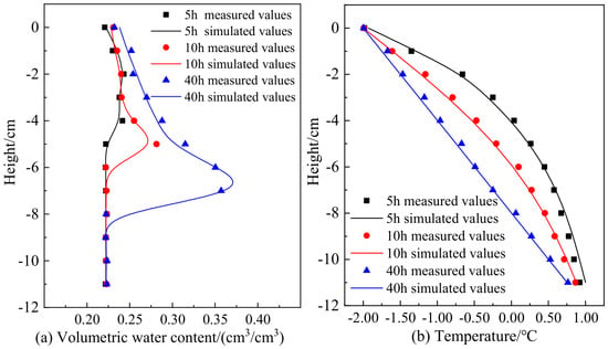
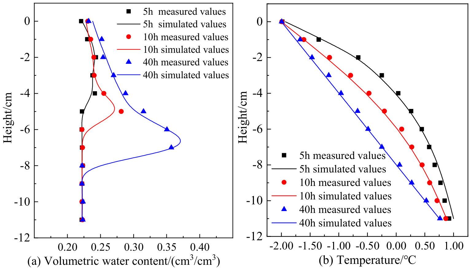
Three replicate one-dimensional freezing tests were conducted on unsaturated clay specimens. Each specimen was 12 cm high and had an initial volumetric water content of 24.0%. The cold-end temperature was −2 °C and the warm-end temperature was 1 °C. During freezing, the specimen sides were thermally insulated and water was continuously supplied without pressure at the bottom. The three specimens were frozen for 5, 10, and 40 h, respectively. After freezing, the volumetric water content was measured using layered sectioning.

A hydro–thermal–mechanical model was established using the preceding theory. The model parameters were consistent with those of the clay used in the laboratory tests (Table 5), and the temperature boundaries were prescribed according to the test conditions. Figure 9 compares measured and simulated volumetric water content and temperature during the one-dimensional freezing tests. The simulated and measured values were reasonably close, indicating that the model captured the principal variable changes during soil freezing to a certain extent.

Table 5. Thermophysical parameters of the clay used in the laboratory test.

Material	λu (W/m·K)	λf (W/m·K)	Cu (J/kg·K)	Cf (J/kg·K)	ρ (kg/m3)	θ0 (m3/m3)
Clay	0.70	2.20	1874	1241	1610	0.24

Figure 9. Comparison of measured and simulated volumetric water content and temperature in one-dimensional freezing tests of soil columns; (a) volumetric water content; (b) temperature.

For quantitative evaluation, the RMSE and MAE of the 36 volumetric water content data points in Figure 9a are approximately 0.0062 and 0.0032 cm³/cm³, respectively; the RMSE and MAE of the 36 temperature data points in Figure 9b are approximately 0.048 and 0.041 °C, respectively. Part of the laboratory test data was also used to determine the clay parameters; therefore, this comparison is a calibration-supported base-model check rather than a fully independent validation.

2.6.2. Validation Against Borehole Data

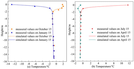
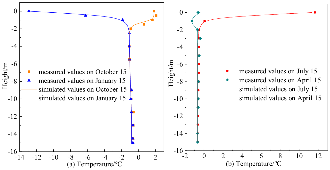
Measured values were obtained from a borehole beneath the natural ground surface along S201 Highway. Follow-up observations were conducted near the middle of January, April, July, and October 2010. Simulated values were taken from the long-term numerical analysis at the corresponding mid-month dates [8,9].

The measured and simulated surface temperatures in July were 11.66 and 11.37 °C, respectively, whereas those in January were −12.91 and −12.76 °C. Both measured and simulated ground temperatures at depths greater than 6 m fell within −0.65 ± 0.02 °C. The close agreement indicates that the model can predict the ground-temperature distribution at this cross-section to a reasonable extent.

For the 51 paired data points in Figure 10a,b, the RMSE and MAE are approximately 0.278 and 0.149 °C, respectively. It should be noted that the 2010–2020 temperature records at the K49 section were also used to fit the upper thermal boundary of the model; therefore, the ground-temperature comparison here is also a calibration-supported consistency check.

Figure 10. Comparison of measured and simulated natural-ground temperature; (a) January and October; (b) April and July.

2.6.3. Mechanical Validation

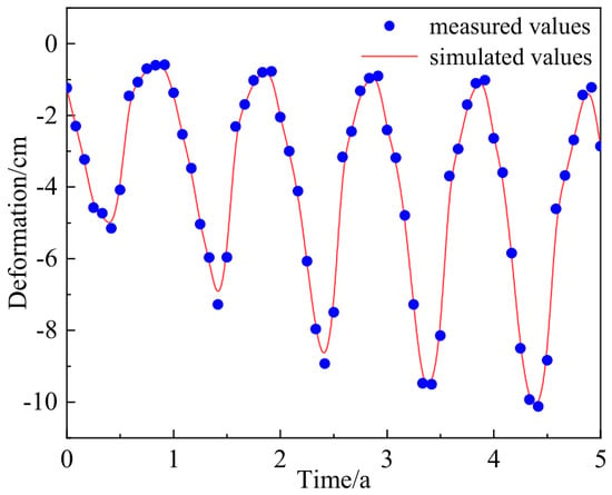
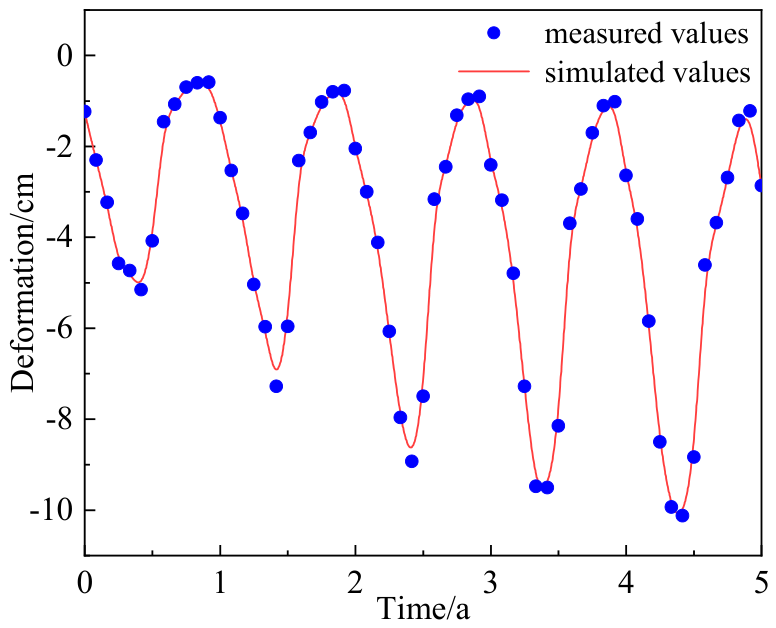
To validate the mechanical model, monitored centerline-deformation data for S201 Highway from 2020 to 2025 were compared with simulated values for the same period. Similar comparisons between simulated and monitored deformation have been used to assess numerical models of permafrost embankments [38]. The road section was constructed in 2009, and 2020 was taken as the initial time in the figure. The simulation and measurements generally agreed in annual cyclic behavior, timing of peaks and troughs, and deformation amplitude. The root-mean-square error (RMSE) was approximately 0.27 cm, indicating that the model adequately represented the long-term deformation characteristics of this cross-section (Figure 11). Centerline deformation from 2020 to 2025 was used to verify the mechanical response. Figure 9, Figure 10 and Figure 11 validate the base HTM framework and the original road-section model, rather than providing field validation of a constructed MSRL project; the MSRL component represents a prediction made on the validated base model.

Figure 11. Comparison of measured and simulated centerline deformation at the K49 cross-section of S201 Highway from 2020 to 2025.

2.6.4. Numerical Discretization Independence Tests

For the mesh independence test, the peak-to-peak amplitude of the vertical displacement at the embankment centerline from 2020 to 2025 was selected as the indicator. With the material parameters, boundary conditions, time-step control, and nonlinear convergence settings unchanged, the coarse, original, and fine meshes contained 550, 940, and 1467 elements, respectively, and yielded displacement amplitudes of 9.83, 9.72, and 9.70 cm. The differences between the coarse and fine meshes relative to the original mesh were 1.13% and 0.20%, respectively; with further refinement, the amplitude changed by only 0.02 cm, indicating that the overall displacement amplitude had essentially stabilized.

Because maximum shear stress is another key indicator used to evaluate the replacement-interface schemes, its mesh sensitivity was further examined for the 1:2.5 case. On 15 October in Year 40, the coarse, original, and fine meshes, containing 550, 940, and 1467 triangular elements, yielded maximum shear stresses of 162, 165, and 167 kPa, respectively. Relative to the original mesh, the differences for the coarse and fine meshes were 1.82% and 1.21%, respectively. Although the number of elements increased by 56.1% from the original mesh to the fine mesh, the maximum shear stress changed by only 2 kPa. Therefore, the original mesh provides sufficiently stable estimates of both the overall displacement amplitude and the maximum shear stress considered in this study.

For the time-step independence test, the mesh, material parameters, boundary conditions, and monthly output times were kept unchanged, and only the maximum internal time step was limited to 1/24 year. Under the original automatic time stepping and the 1/24 year limit, the peak-to-peak amplitudes of the centerline vertical displacement from 2020 to 2025 were 9.72 and 9.67 cm, respectively, with an absolute difference of 0.05 cm and a relative difference of 0.51% from the original setting. This indicates that further reducing the internal time step has only a small effect on the displacement amplitude.

3. Results

The permafrost table in the study area generally reaches its maximum annual depth in October; accordingly, its position was approximated by the 0 °C isotherm on 15 October. The results first compare ground temperature, volumetric ice content, and long-term deformation between the unprotected embankment and the MSRE, then examine slope-toe deformation in the MSRE and rectangular rockfill embankment, and finally compare the stress and temperature responses for different replacement-interface slopes.

3.1. Ground-Temperature and Ice-Content Distributions Beneath the Unprotected Embankment

The permafrost beneath the unprotected embankment degraded continuously with service time. Because the right slope received stronger solar radiation, thawing was more pronounced beneath that side.

In Year 4, the 0 °C isotherm already exhibited marked lateral nonuniformity (Figure 12a). Its depths beneath the natural ground surface and the embankment centerline were approximately 1.88 and 2.39 m, respectively; the corresponding depths beneath the right and left slope toes were approximately 3.50 and 2.32 m, a difference of 1.18 m. Zones with a volumetric ice content above 0.12 occurred mainly below a depth of approximately 2.21 m and within the horizontal ranges X = 15–42 m and X = 45–60 m (Figure 12b).

Figure 12. Temperature and volumetric ice-content distributions beneath the unprotected embankment: (a) temperature on 15 October in Year 4; (b) volumetric ice content on 15 October in Year 4; (c) temperature on 15 October in Year 40; (d) volumetric ice content on 15 October in Year 40.

By Year 40, the extent of permafrost degradation had increased markedly, and the lateral difference had become more pronounced. The 0 °C isotherm was approximately 3.64 m below the natural ground surface and 7.98 m below the embankment centerline. At the centerline, it had descended by 5.59 m since Year 4, corresponding to an average rate of approximately 0.16 m/a. Its depths beneath the right and left slope toes were approximately 6.20 and 4.46 m, respectively, increasing their difference to 1.74 m (Figure 12c). Zones with a volumetric ice content above 0.12 retreated to approximately 4 m below the ground surface and were restricted to local areas at X = 15–27 m and X = 46–60 m (Figure 12d). These changes indicate that persistent heat accumulation reduced the thermal stability of the underlying permafrost.

3.2. Ground-Temperature and Ice-Content Distributions Beneath the MSRE

The MSRL substantially limited degradation of the underlying permafrost and mitigated the asymmetric degradation caused by unequal heat input from the two side slopes.

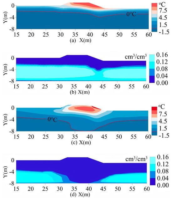
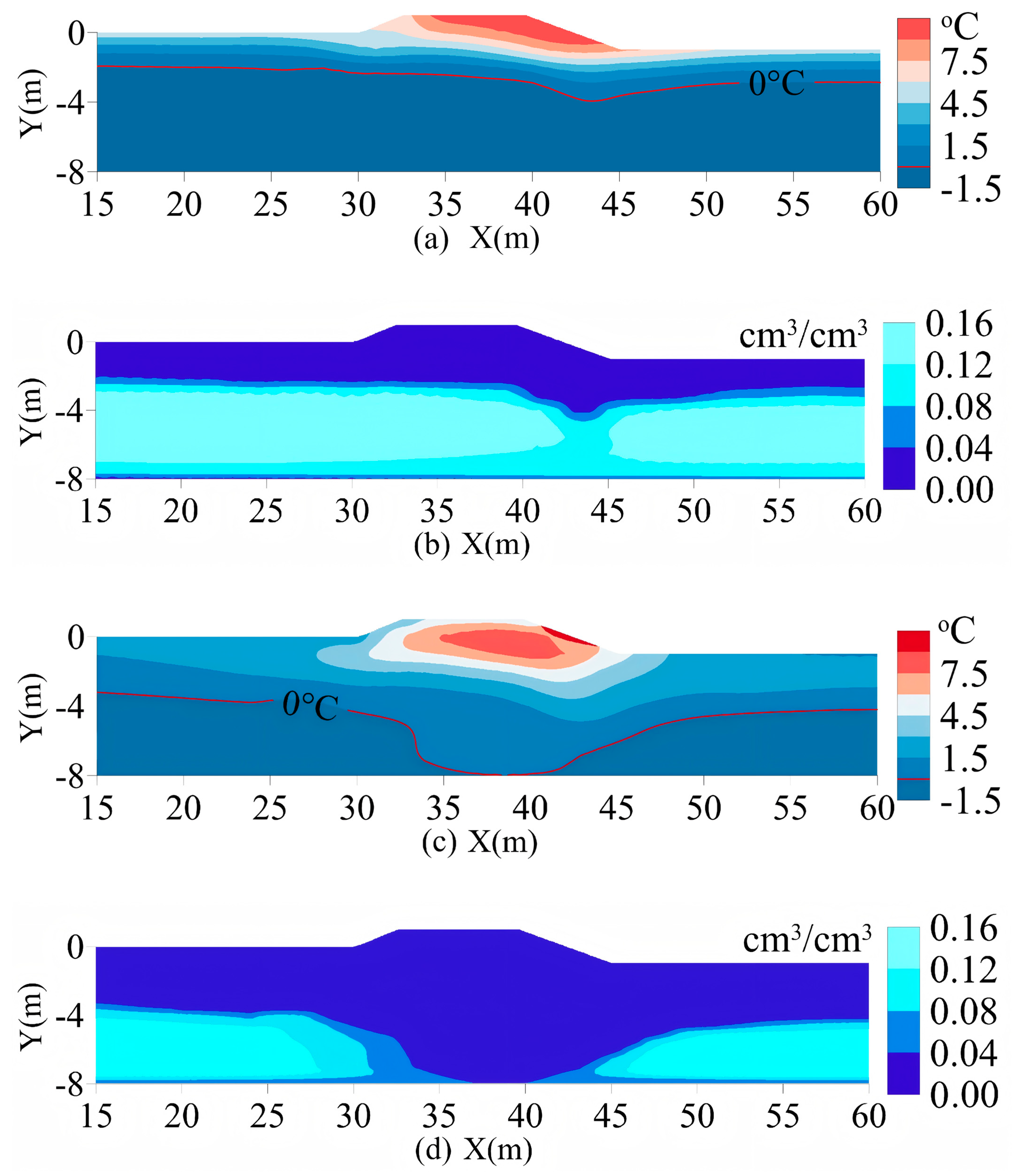
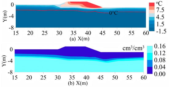
In Year 4, the permafrost-table depth beneath the MSRE centerline was close to that beneath the unprotected embankment. The depths of the 0 °C isotherm beneath the natural ground surface and embankment centerline were approximately 1.74 and 2.50 m, respectively. Its depth beneath the right slope toe was approximately 2.23 m, which was 1.27 m shallower than the 3.50 m depth beneath the unprotected embankment (Figure 13a). The zone with a volumetric ice content above 0.12 occurred mainly below a depth of approximately 2.13 m and extended across the entire cross-section from X = 15 to 60 m (Figure 13b).

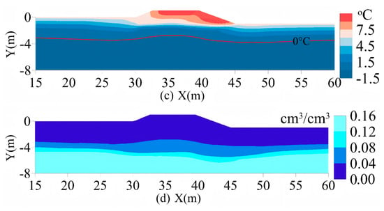
Figure 13. Temperature and volumetric ice-content distributions beneath the MSRE: (a) temperature on 15 October in Year 4; (b) volumetric ice content on 15 October in Year 4; (c) temperature on 15 October in Year 40; (d) volumetric ice content on 15 October in Year 40.

By Year 40, the MSRE continued to limit both downward migration of the permafrost table and lateral nonuniformity. The 0 °C isotherm was approximately 3.62 m below the natural ground surface and 3.27 m below the embankment centerline. At the centerline, it had descended by only 0.77 m since Year 4, corresponding to an average rate of approximately 0.02 m/a, markedly lower than the 0.16 m/a beneath the unprotected embankment. Its depths beneath the right and left slope toes were approximately 3.34 and 3.65 m, respectively, a difference of 0.31 m—approximately 82% smaller than the 1.74 m difference beneath the unprotected embankment (Figure 13c).

The volumetric ice-content distribution also indicates that the frozen ground beneath the MSRE remained comparatively well preserved. In Year 40, the zone with a volumetric ice content above 0.12 occurred mainly below a depth of approximately 3.81 m and extended across the entire cross-section, whereas only local zones on both sides remained beneath the unprotected embankment. In particular, the volumetric ice content beneath the right slope toe of the MSRE remained above 0.12, and the corresponding ice-rich zone remained continuous (Figure 13d).

3.3. Long-Term Deformation of the MSRE

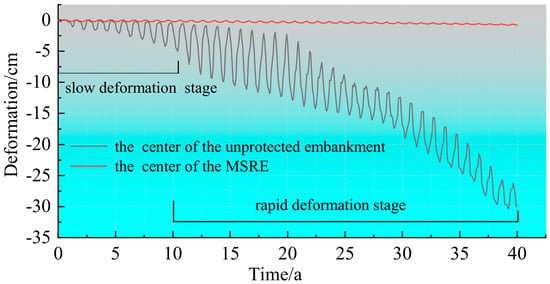
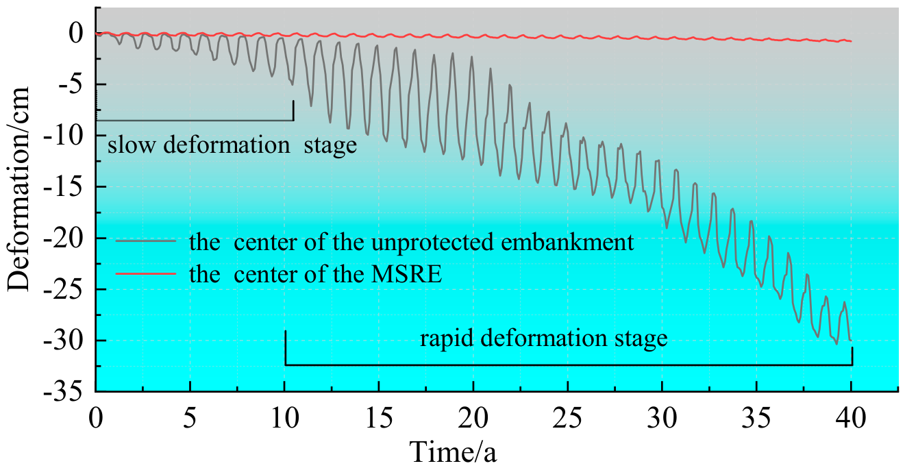
The MSRE substantially reduced long-term settlement at the embankment centerline and did not exhibit the rapid late-stage deformation observed in the unprotected embankment (Figure 14).

Figure 14. Centerline vertical-deformation curves for the MSRE and unprotected embankment.

During the first 10 years, cumulative settlement of the unprotected embankment was approximately 2.65 cm, corresponding to a relatively low average rate of 0.27 cm/a. Between Years 10 and 40, cumulative settlement increased from 2.65 to 29.2 cm, and the average rate increased to 0.89 cm/a. By contrast, cumulative settlement of the MSRE was only 0.86 cm after 40 years, approximately 97.1% lower than that of the unprotected embankment, and its seasonal fluctuations remained small throughout the simulation.

3.4. Comparison of Slope-Toe Deformation Between the MSRE and Rectangular Rockfill Embankment

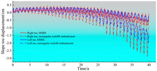
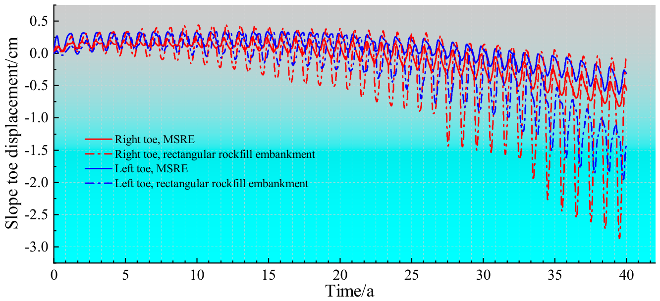
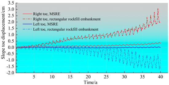
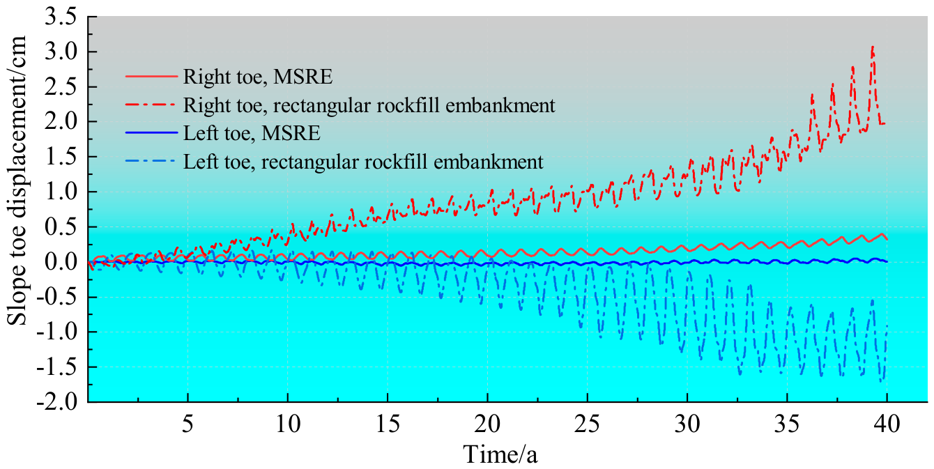
Differences between the two replacement schemes emerged mainly in intermediate- and late-stage slope-toe deformation: settlement and outward displacement accumulated continuously in the rectangular scheme, whereas both remained small in the MSRE (Figure 15 and Figure 16).

Figure 15. Vertical displacements at the slope toes of the two rockfill embankments.

Figure 16. Horizontal displacements at the slope toes of the two rockfill embankments.

Negative vertical displacement denotes settlement, whereas positive and negative horizontal displacements denote rightward and leftward movement, respectively. In Year 40, the vertical displacements at the right and left slope toes of the rectangular rockfill embankment were −2.92 and −1.91 cm, respectively, and the corresponding horizontal displacements were 3.22 and −1.75 cm, indicating outward movement on both sides. During the same period, the vertical displacements at the right and left slope toes of the MSRE were −0.82 and −0.62 cm, and the corresponding horizontal displacements were 0.32 and −0.07 cm.

3.5. Hydro–Thermal–Mechanical Responses for Different Replacement-Interface Slopes

The replacement-interface slope primarily affects stress concentration at the rockfill–clay interface and temperature fluctuations near the slope toes. To control other factors, the vertical, 1:1.5, 1:2.5, and 1:3.5 interfaces were compared under identical material parameters, boundary conditions, replacement-layer top width, and maximum replacement depth (Figure 7). Maximum shear stress on 15 October in Year 40 was used to characterize the mechanical response, and temperature 3 m below the right slope toe was used to characterize the thermal response.

$${\tau }_{max}={\displaystyle \frac{{\sigma }_1-{\sigma }_3}{2}}.$$

(40)

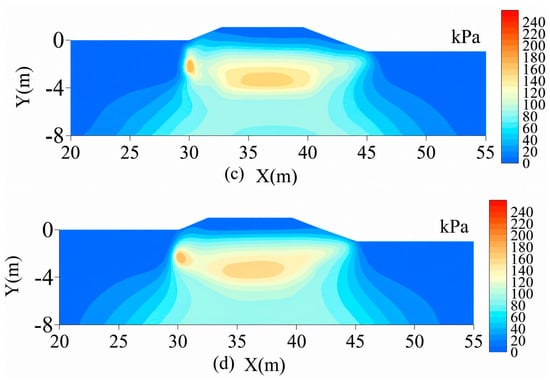
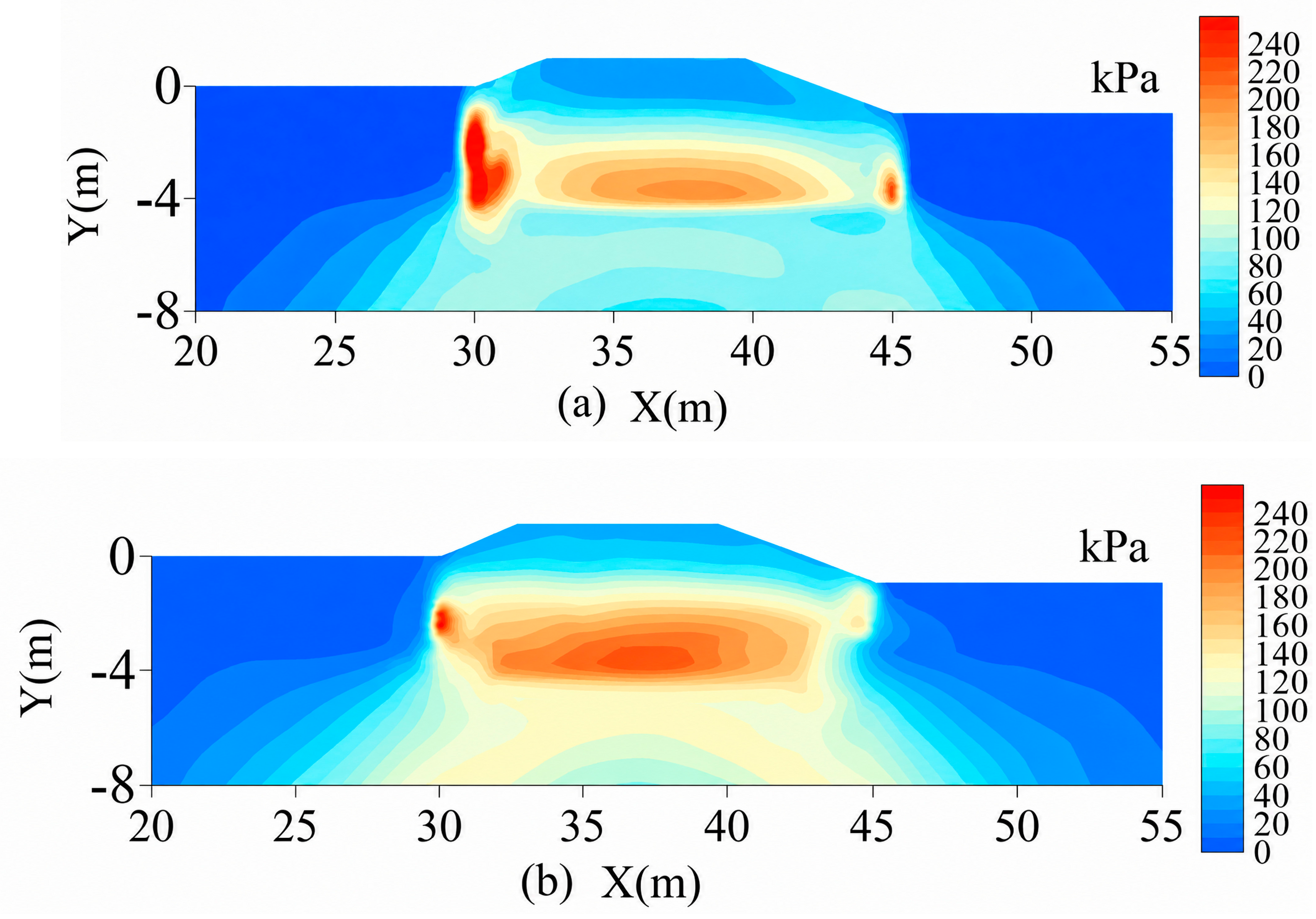
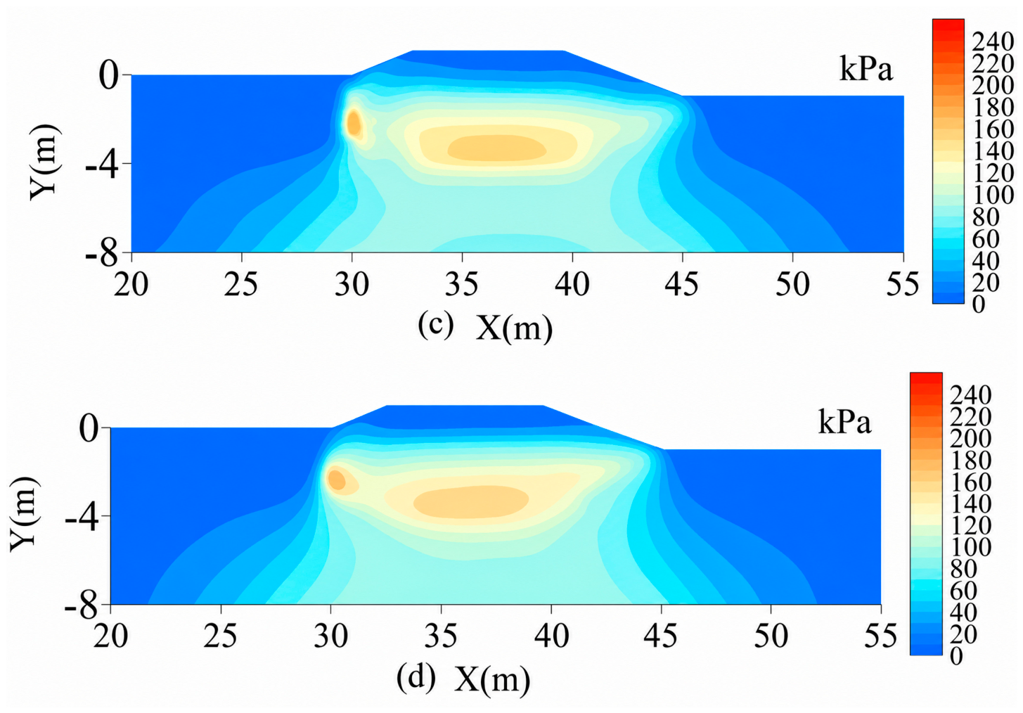
The peak maximum shear stresses for the vertical, 1:1.5, 1:2.5, and 1:3.5 interfaces were 236, 224, 165, and 159 kPa, respectively, corresponding to reductions of 5.1%, 30.1%, and 32.6% for the latter three cases relative to the vertical interface. For the vertical and 1:1.5 interfaces, the high-stress zones were concentrated mainly along the left-side and bottom interfaces, where maximum shear stress was approximately 190–240 kPa over the principal zones. For the 1:2.5 interface, the high-stress zones contracted markedly, and maximum shear stress over the principal zones decreased to approximately 110–170 kPa. The distribution for the 1:3.5 interface was similar to that for the 1:2.5 interface, with a further peak reduction of only 3.6% (Figure 17).

Figure 17. Maximum shear-stress distributions on 15 October in Year 40 for different replacement-interface slopes: (a) vertical interface; (b) 1:1.5; (c) 1:2.5 (MSRL); (d) 1:3.5.

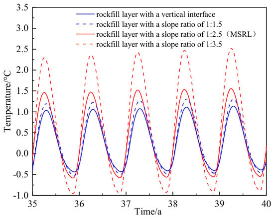
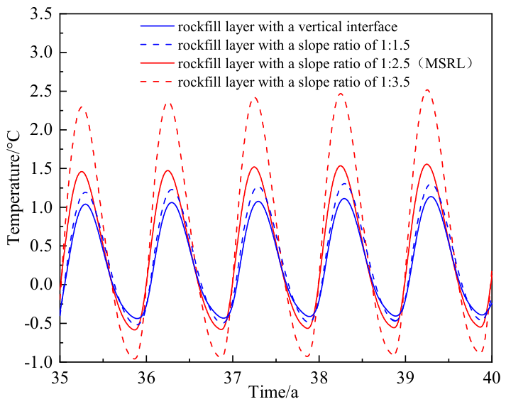
Slope-toe temperature fluctuations generally increased as the replacement interface became flatter, with the most pronounced fluctuations occurring for the 1:3.5 case (Figure 18). From Years 35 to 40, all cases exhibited similar annual-cycle phases and a slight overall warming trend. The annual maximum temperatures for the vertical, 1:1.5, 1:2.5, and 1:3.5 interfaces were approximately 1.1, 1.3, 1.6, and 2.6 °C, respectively; the corresponding annual minimum temperatures were approximately −0.5, −0.4, −0.6, and −0.8 °C, yielding annual temperature ranges of approximately 1.6, 1.8, 2.2, and 3.4 °C. Relative to the 1:2.5 case, the 1:3.5 case increased the annual maximum temperature by approximately 1.0 °C and the annual temperature range by approximately 1.2 °C.

Figure 18. Temperature histories 3 m below the right slope toe for different replacement-interface slopes (Years 35–40).

4. Discussion

4.1. Mechanisms of the MSRL

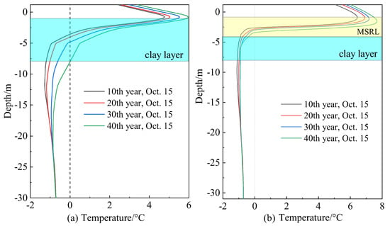
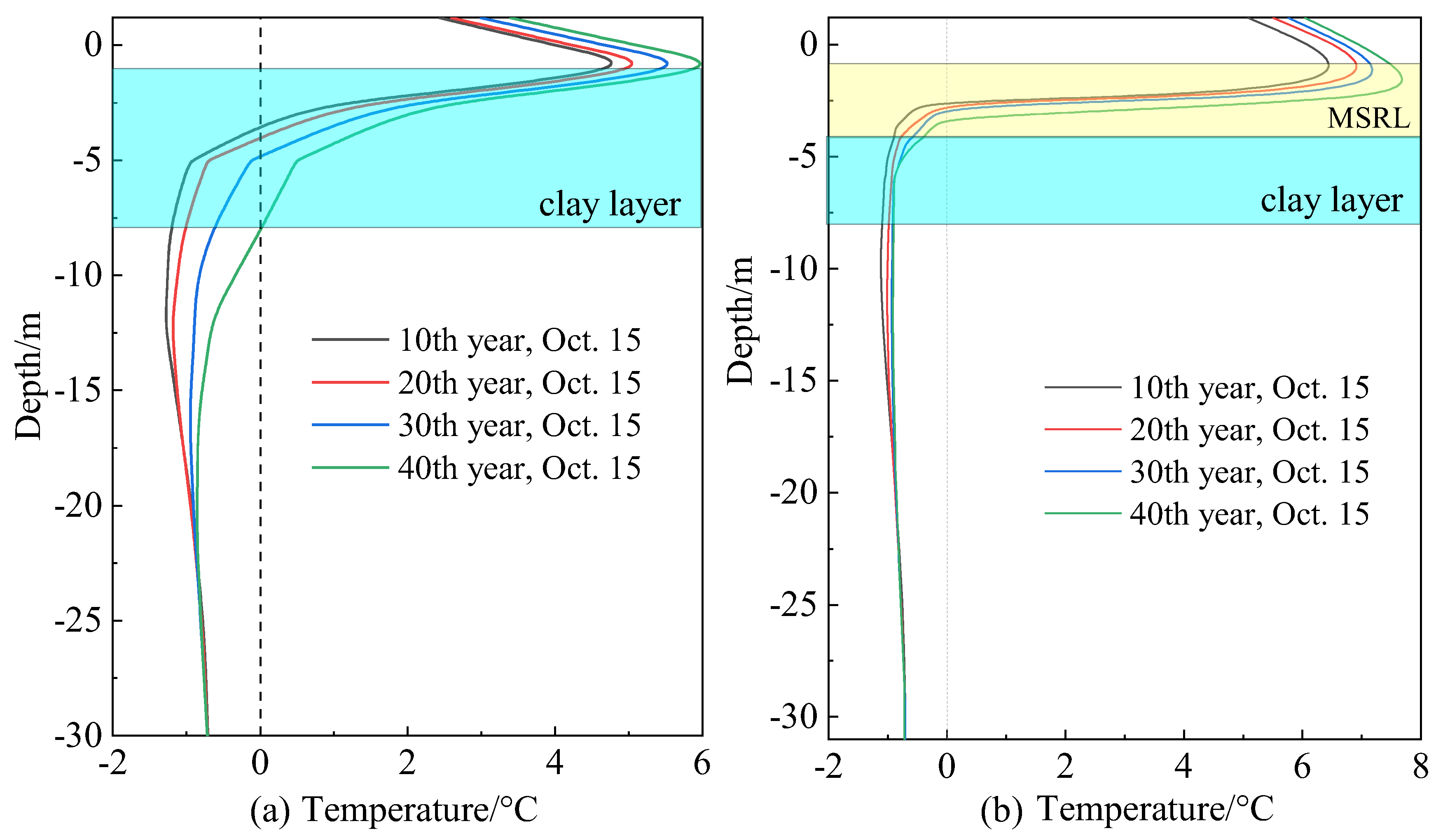
The accelerated late-stage settlement of the unprotected embankment was primarily associated with stiffness loss caused by warming and thawing of the underlying frozen clay. The permafrost-table depths beneath the centerline in Years 10, 20, 30, and 40 were 3.21, 3.52, 4.34, and 7.98 m, respectively, indicating continuous downward migration and progressive deepening of the thawed clay layer. As the clay temperature approached and entered the critical freeze–thaw interval from −1 to 0 °C, its elastic modulus decreased from approximately 6.0 to 3.2 MPa, while cohesion decreased from approximately 0.898 to 0.068 MPa. The combined loss of stiffness and strength accelerated deformation [38,39].

The MSRL first limits permafrost degradation by slowing warm-season heat transfer to greater depths [8,9]. Unlike conventional crushed-rock cooling embankments that place porous rock layers at the embankment base and/or on the slopes to enhance heat dissipation [10,12,14], the MSRL is formed primarily by excavating and replacing weak foundation clay; therefore, its engineering function also includes direct mechanical improvement of the subgrade. Under the equivalent thermal properties adopted in this study, the depths of the 0 °C isotherm beneath the MSRE centerline on 15 October in Years 10, 20, 30, and 40 were 2.65, 2.77, 2.94, and 3.27 m, respectively, markedly shallower than the corresponding depths beneath the unprotected embankment (3.21, 3.52, 4.34, and 7.98 m). Moreover, on 15 October in Year 40, the clay beneath the MSRL generally remained below 0 °C and experienced substantially less warming than that beneath the unprotected embankment (Figure 19), indicating that the MSRL maintained the thermal stability of the warm permafrost.

Figure 19. Centerline temperature profiles: (a) unprotected embankment; (b) MSRE. The horizontal dotted line indicates the clay–tuff interface.

The MSRL also replaces part of the low-modulus clay, increasing the stiffness of the subgrade beneath the embankment and reducing the thickness of the underlying clay layer [8,40]. Through the combined effects of thermal protection and mechanical replacement, centerline settlement of the MSRE was limited to 0.86 cm in Year 40, far below the 29.2 cm settlement of the unprotected embankment.

4.2. Comparison Between the MSRE and the Rectangular Rockfill Embankment

For the two schemes considered in this study, the principal advantage of the MSRL over the rectangular rockfill layer was improved long-term control of slope-toe deformation. The schemes differed not only in side-interface geometry but also in lateral replacement extent and rockfill consumption. Therefore, the following comparison assumes an identical design thickness and evaluates the overall mechanical and thermal performance of the complete MSRL and rectangular rockfill schemes; the observed differences cannot be attributed to interface geometry alone.

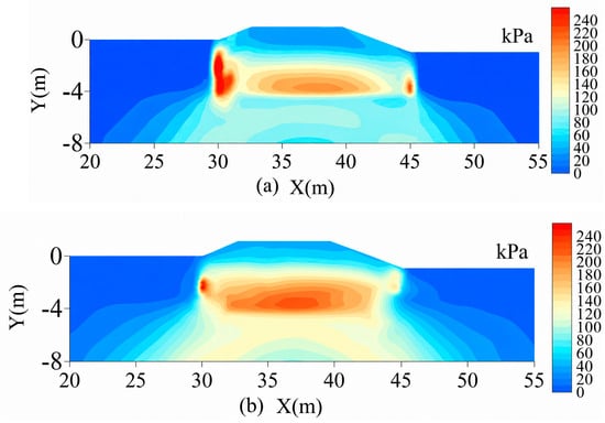
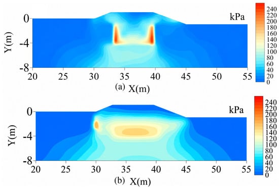
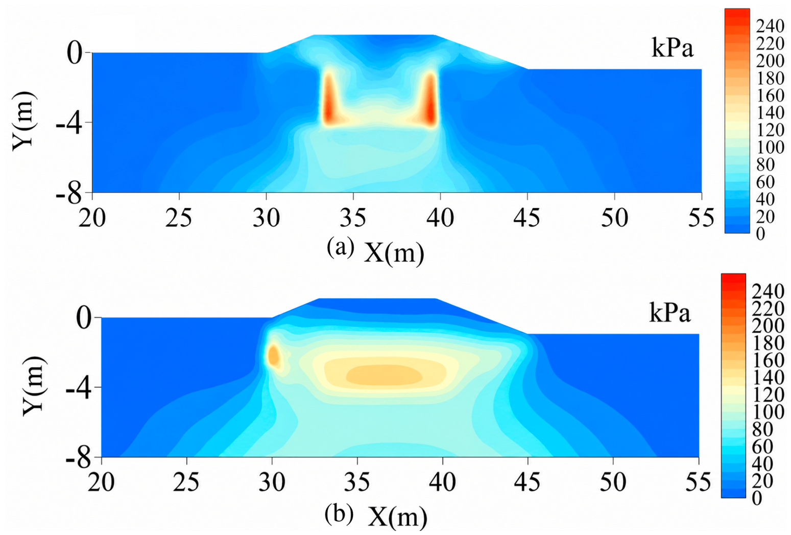
Mechanically, the inclined sides of the MSRL follow the embankment slope ratio, increasing the rockfill–clay contact area and reducing local stress concentration. The maximum shear stress in the rectangular rockfill embankment was 247 kPa, with high values concentrated along the vertical rockfill–clay interface and densely spaced, sharply curved contours. The corresponding peak in the MSRE was 165 kPa, and its high-stress zone was smaller with more continuous contours (Figure 20). In the rectangular scheme, the vertical side interface forms a distinct corner with the bottom interface. Under loading, deformation incompatibility between the rockfill and clay tends to concentrate near this corner and produce locally high stresses. The inclined MSRL interface lengthens and smooths the transition between the two materials, resulting in a more uniform stress distribution. This pattern is consistent with the smaller horizontal displacement at the MSRE slope toes and indicates better control of outward slope-toe deformation.

Figure 20. Maximum shear-stress distributions on 15 October in Year 40: (a) rectangular rockfill embankment; (b) MSRE.

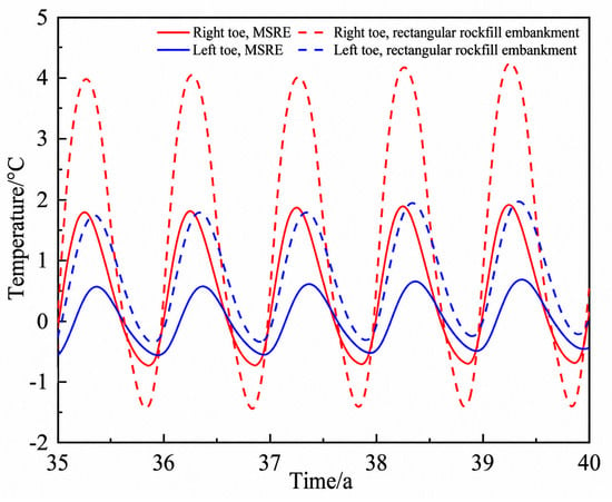
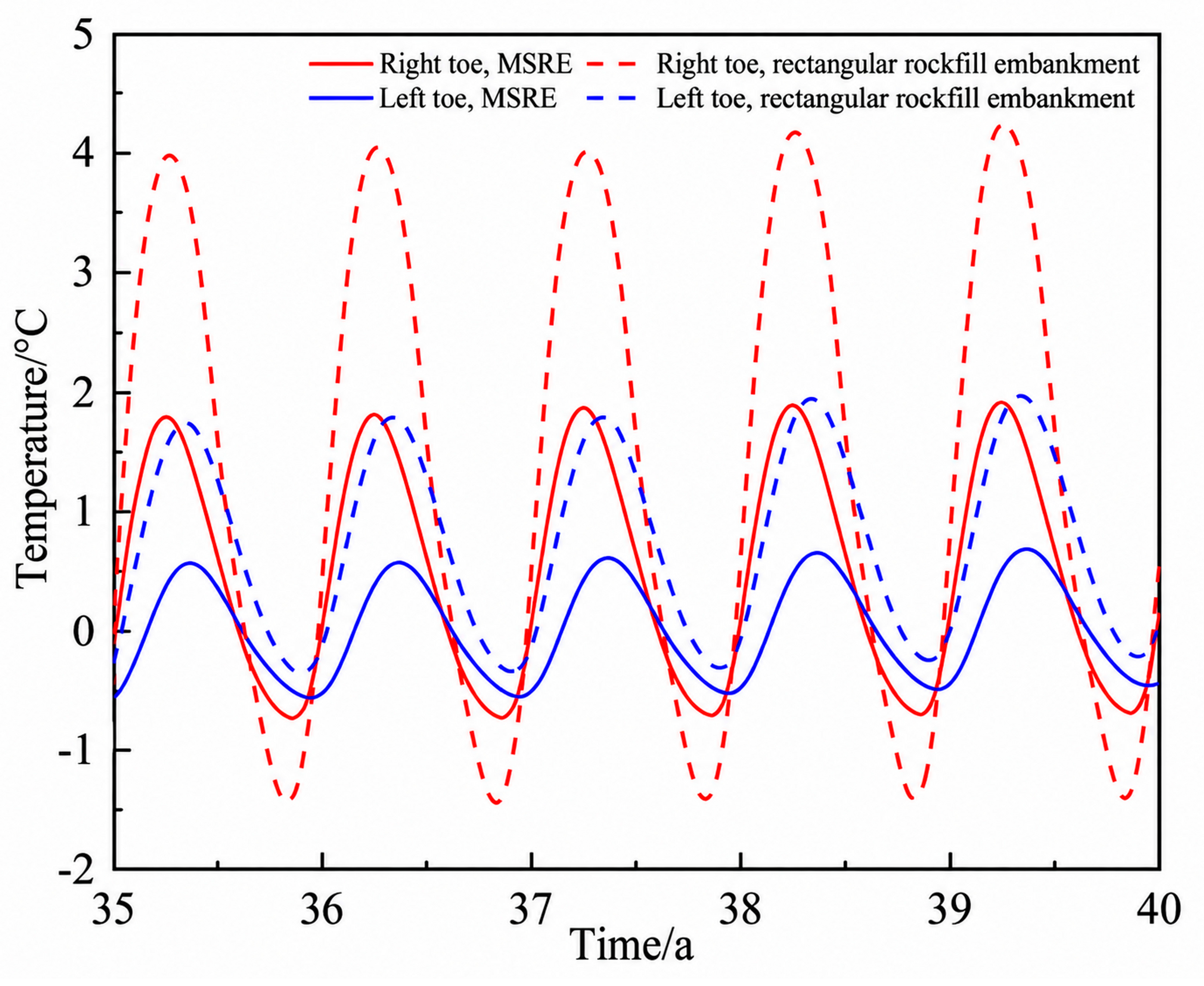
Thermally, the MSRL reduced the unreplaced clay area near the slope toes and thereby limited local heat input. Under the equivalent thermal parameters adopted in this study, the annual temperature ranges 3 m below the right and left slope toes of the rectangular rockfill embankment in Year 40 were 5.8 and 2.3 °C, respectively; the corresponding values for the MSRE decreased to 2.2 and 1.1 °C (Figure 21). Continuous coverage along the slope profile therefore moderated temperature variations near the slope toes and reduced the difference between the two sides.

Figure 21. Temperature histories 3 m below the slope toes of the two rockfill embankments (Years 35–40).

To more directly compare the influence of interface geometry, the 15 m wide vertical-interface scheme in Figure 7a was also compared with the 1:2.5 MSRL under an equal lateral replacement extent. On 15 October in Year 40, their maximum shear stresses were 236 and 165 kPa, respectively, with the MSRL reducing it by 30.1%; the rockfill consumption decreased from 48.00 to 40.15 m³/m, a reduction of 16.4% (Figure 7 and Figure 17). However, the annual temperature variation range at 3 m below the right slope toe increased from 1.6 to 2.2 °C (Figure 18). Therefore, the inclined interface is more favorable in terms of stress concentration and material consumption, but the local temperature fluctuation increases slightly; this is a trade-off among several performance indicators rather than a comprehensive superiority over the rectangular scheme in all aspects.

4.3. Basis for Selecting the MSRL Among the Four Candidate Interface Slopes

The four candidate cases indicate that the 1:2.5 interface provides a favorable balance among stress reduction, temperature fluctuation, and rockfill consumption. As the interface was progressively flattened from vertical, stress concentrations continued to decrease; however, the local replacement layer became thinner and slope-toe temperature fluctuations increased.

Mechanically, flattening the interface lengthened the load-transfer path and allowed stress to redistribute over a wider area. At the vertical interface (1:0), the stiffness contrast between the materials coincided with a geometric discontinuity, promoting a localized high-shear-stress zone as load was transferred from the rockfill layer to the clay foundation. Because the transition remained short for the 1:1.5 interface, its maximum shear stress was only 5.1% lower than that of the 1:0 case. At 1:2.5, the maximum shear stress was 26.3% lower than that of the 1:1.5 case, and the high-stress zone contracted markedly. Further flattening to 1:3.5 reduced the maximum shear stress by only an additional 3.6%, indicating substantially diminishing mechanical benefits beyond 1:2.5.

Thermally, an excessively flat interface thinned the rockfill layer near the slope toe and increased seasonal subgrade-temperature variations. For the temperature 3 m below the right slope toe examined in Section 3.5, the 1:2.5 case produced slightly larger but numerically comparable fluctuations relative to the 1:0 and 1:1.5 cases. After the interface was flattened to 1:3.5, the warm-season maximum temperature increased by approximately 1.0 °C and the annual temperature range increased by approximately 1.2 °C relative to the 1:2.5 case.

In terms of replacement volume per longitudinal meter of embankment, the vertical, 1:1.5, 1:2.5, and 1:3.5 cases required 48.00, 43.29, 40.15, and 37.01 m³/m of rockfill, respectively. The 1:2.5 case used 16.4% less rockfill than the vertical case and 7.3% less than the 1:1.5 case. Although the 1:3.5 case saved a further 3.14 m³/m, its additional mechanical benefit was limited and its temperature fluctuations increased markedly.

To reduce the bias caused by judgment based on a single indicator, a simple normalized comprehensive evaluation was performed for the four schemes using the maximum shear stress τ_max, the annual temperature variation range ΔT at 3 m below the right slope toe from Years 35–40, and the rockfill consumption per linear meter V. All three indicators are such that smaller values are more favorable, and min–max normalization was adopted:

$$N_{ij}={\displaystyle \frac{X_{j,max}-X_{ij}}{X_{j,max}-X_{j,min}}},0\le N_{ij}\le 1$$

(41)

where x_ij is the original value of the j-th indicator for the i-th scheme, and x_i,max and x_i,min are the maximum and minimum values of that indicator among the four schemes, respectively. A larger N_ij indicates better performance of the corresponding indicator. Because no objective basis for weighting is available, the three indicators were assigned equal weights of 1/3. The composite score is:

$$S_i={\displaystyle \frac{N_{i,\tau max}+N_{i,T}+N_{i,V}}{3}}$$

(42)

Table 6 shows that the equal-weight composite scores of the vertical, 1:1.5, 1:2.5, and 1:3.5 schemes are 0.333, 0.491, 0.768, and 0.667, respectively, with 1:2.5 ranking first among the four discrete schemes. When the interface slope was further flattened from 1:2.5 to 1:3.5, the maximum shear stress decreased by only an additional 3.6%, while the annual temperature variation range increased from 2.2 to 3.4 °C, an increase of 54.5% (Figure 17 and Figure 18). This indicates that 1:2.5 does not minimize every indicator but rather achieves a more balanced performance among the three indicators.

Table 6. Normalized multi-criteria evaluation of schemes with different interface slopes.

Interface Slope Ratio	τmax/kPa (Nτ)	ΔT/°C (NT)	V/(m3/m) (NV)	S	Rank
Vertical interface (1:0)	236 (0.000)	1.6 (1.000)	48.00 (0.000)	0.333	4
1:1.5	224 (0.156)	1.8 (0.889)	43.29 (0.429)	0.491	3
1:2.5	165 (0.922)	2.2 (0.667)	40.15 (0.714)	0.768	1
1:3.5	159 (1.000)	3.4 (0.000)	37.01 (1.000)	0.667	2

In the weight sensitivity test, when the weight of any one indicator was increased to 0.50 and the other two were each set to 0.25, the scores of 1:2.5 were 0.806, 0.742, and 0.754, respectively, and it remained ranked first in all cases. When the weight of material consumption was 0.50, the scores of 1:2.5 and 1:3.5 were very close (0.754 and 0.750), indicating that the preferred selection still varies with engineering objectives. Therefore, 1:2.5 can only be regarded as the preferred scheme under the engineering conditions of this study and among the four discrete schemes, rather than the global optimum over a continuous range of slope ratios.

The 1:2.5 interface is explicitly conditional and should not be regarded as a global optimum over a continuous range of slopes. It is applicable only to road sections broadly comparable to the present case in terms of the 1:2.5 upper embankment slope, 3.2 m design replacement thickness, stratigraphy, and climatic boundaries. When embankment height, natural-ground inclination, replacement thickness, rockfill properties, foundation ice content, or temperature boundaries differ substantially, the design should be recalculated and checked against replacement volume per unit length and construction conditions.

4.4. Engineering Significance and Model Limitations

The engineering significance of the MSRL lies in extending continuous rockfill protection to the embankment slope toes, thereby providing a passive measure that addresses both thermal stability and deformation control in warm island permafrost. The MSRL is not intended to replace the rectangular rockfill layer in all cases; rather, it supplements existing rockfill-replacement methods by targeting vulnerable slope-toe zones and provides a basis for selecting the replacement extent and structural form for similar road sections.

The limitations of this study mainly arise from model dimensionality, physical processes, and parameter assumptions. The two-dimensional cross-sectional model does not account for longitudinal terrain variation or end effects, and the hydrothermal processes do not explicitly include water vapor migration [41]. Material parameters and the warming boundary are also treated as deterministic values. The Drucker–Prager model adopts an associated flow rule with ψ(T) = φ(T); this is a common first-order simplification, but it may overestimate dilatancy and plastic volumetric strain in localized shear zones [21,22].

In this study, the MSRL is a buried, enclosed structure, and its 3.2 m thickness may induce natural convection driven by temperature differences. However, the MSRL was modeled primarily as a pure heat conduction medium in the simulation. Therefore, neglecting local natural convection may cause the simulated winter temperatures to be slightly higher, leading to a conservative estimate of the absolute cooling effect [42]. On the other hand, the fitted temperature boundary only partially incorporates the integrated effects of historical snow cover from 2010 to 2020; if future snow cover becomes thicker or persists longer, the model may overestimate winter heat dissipation, resulting in lower ground temperatures and smaller thaw settlement [31].

The continuous-interface assumption facilitates comparison of geometric schemes under uniform conditions, but it cannot describe local slip, opening, fine-particle migration, or clogging. Previous experiments have observed progressive erosion at soil–rock interfaces as the hydraulic gradient increases [43]. No geotextile was included in the present model because interface parameters, as well as 40-year data on construction damage, clogging, and degradation for this project, are still lacking. The placement and compaction of coarse-grained material may cause geotextile abrasion or puncture [44,45]. In actual engineering, a graded filter transition layer can be installed according to site-specific soil and hydraulic conditions [46], or a high-strength geotextile with a protective cushion can be adopted; the specific configuration should be determined through filter compatibility and construction durability tests.

Future research will incorporate long-term field monitoring and multi-section data, gradually adding three-dimensional terrain, air–thermal coupling within the rockfill layer, a dynamic snow cover layer, interface contact and particle erosion, and will conduct sensitivity and uncertainty analyses of key parameters.

5. Conclusions

(1)

Long-term warming caused continuous degradation of the permafrost beneath the unprotected embankment, with centerline settlement reaching 29.20 cm in Year 40. With the MSRL, the centerline permafrost table descended by only 0.77 m from Years 4 to 40, and cumulative settlement in Year 40 was 0.86 cm, indicating that the MSRL can provide long-term control of permafrost degradation and embankment settlement.

(2)

Compared with the conventional rectangular rockfill layer, the MSRL provided better control of slope-toe temperature and deformation. In Year 40, the annual temperature range 3 m below the right slope toe decreased by 3.6 °C, while the absolute vertical and horizontal displacements at the right slope toe decreased by 2.10 and 2.90 cm, respectively. The principal advantage of the MSRL is therefore its long-term control of slope-toe temperature and deformation.

(3)

Among the vertical, 1:1.5, 1:2.5 (MSRL), and 1:3.5 interfaces, the 1:2.5 case reduced maximum shear stress by 30.1% and rockfill consumption by 16.4% relative to the vertical case. Further flattening to 1:3.5 reduced maximum shear stress by only an additional 3.6% but increased the annual slope-toe temperature range by 1.2 °C. Under the engineering conditions investigated, the 1:2.5 mirror slope therefore provides a reasonable balance among mechanical response, thermal control, and rockfill consumption and can inform embankment design in warm island permafrost environments.

References

- Li, X.; Cheng, G.; Jin, H.; Kang, E.; Che, T.; Jin, R.; Wu, L.; Nan, Z.; Wang, J.; Shen, Y. Cryospheric change in China. Glob. Planet. Chang. 2008, 62, 210–218. [Google Scholar] [CrossRef] [Scilit]
- Biskaborn, B.K.; Smith, S.L.; Noetzli, J.; Matthes, H.; Vieira, G.; Streletskiy, D.A.; Schoeneich, P.; Romanovsky, V.E.; Lewkowicz, A.G.; Abramov, A.; et al. Permafrost is warming at a global scale. Nat. Commun. 2019, 10, 264. [Google Scholar] [CrossRef] [Scilit] [PubMed]
- Zhang, Z.-Q.; Wu, Q.-B.; Hou, M.-T.; Tai, B.-W.; An, Y.-K. Permafrost change in Northeast China in the 1950s–2010s. Adv. Clim. Chang. Res. 2021, 12, 18–28. [Google Scholar] [CrossRef] [Scilit]
- Wang, X.; Li, X.; Wang, W.; Wang, Z.; Ding, L.; Song, Y.; Liu, Y. The spatial and temporal distribution of permafrost in Northeast China based on temperature at the top of permafrost model. For. Eng. 2025, 41, 990–999. [Google Scholar] [CrossRef]
- Chang, X.; Jin, H.; He, R.; Zhang, Y.; Li, X.; Jin, X.; Li, G. Permafrost changes in the northwestern Da Xing’anling Mountains, Northeast China, in the past decade. Earth Syst. Sci. Data 2022, 14, 3947–3959. [Google Scholar] [CrossRef] [Scilit]
- Hjort, J.; Streletskiy, D.; Doré, G.; Wu, Q.; Bjella, K.; Luoto, M. Impacts of permafrost degradation on infrastructure. Nat. Rev. Earth Environ. 2022, 3, 24–38. [Google Scholar] [CrossRef] [Scilit]
- Ran, Y.; Cheng, G.; Dong, Y.; Hjort, J.; Lovecraft, A.L.; Kang, S.; Tan, M.; Li, X. Permafrost degradation increases risk and large future costs of infrastructure on the Third Pole. Commun. Earth Environ. 2022, 3, 238. [Google Scholar] [CrossRef] [Scilit]
- Shan, W.; Ma, M.; Guo, Y.; Zhang, C. Numerical analysis of the influence of foundation replacement materials on the hydrothermal variation and deformation process of highway subgrades in permafrost regions. Water 2022, 14, 2642. [Google Scholar] [CrossRef] [Scilit]
- Shan, W.; Li, Y.; Guo, Y.; Zhang, C.; Hou, P. Ground temperature monitoring and simulation of temperature field changes in block-stone material replacement foundation for the Shiwei–Labudalin Highway. Appl. Sci. 2024, 14, 6222. [Google Scholar] [CrossRef] [Scilit]
- Cheng, G. A roadbed cooling approach for the construction of Qinghai–Tibet Railway. Cold Reg. Sci. Technol. 2005, 42, 169–176. [Google Scholar] [CrossRef] [Scilit]
- Liu, M.; Niu, F.; Ma, W.; Fang, J.; Lin, Z.; Luo, J. Experimental investigation on the enhanced cooling performance of a new crushed-rock revetment embankment in warm permafrost regions. Appl. Therm. Eng. 2017, 120, 121–129. [Google Scholar] [CrossRef] [Scilit]
- Pei, W.; Zhang, M.; Li, S.; Lai, Y.; Jin, L. Thermo-mechanical stability analysis of cooling embankment with crushed-rock interlayer on a sloping ground in permafrost regions. Appl. Therm. Eng. 2017, 125, 1200–1208. [Google Scholar] [CrossRef] [Scilit]
- Ma, Q.; Luo, X.; Gao, J.; Sun, W.; Li, Y.; Lan, T. Numerical evaluation for cooling performance of a composite measure on expressway embankment with shady and sunny slopes in permafrost regions. Energy 2022, 244, 123194. [Google Scholar] [CrossRef] [Scilit]
- Guo, Y.; Pei, W.; Zhang, M.; Liu, D.; Bai, R.; Zhou, Y.; Li, G. Numerical study on cooling performance of the L-shaped crushed-rock embankment in permafrost regions. Cold Reg. Sci. Technol. 2025, 230, 104380. [Google Scholar] [CrossRef] [Scilit]
- Harlan, R.L. Analysis of coupled heat-fluid transport in partially frozen soil. Water Resour. Res. 1973, 9, 1314–1323. [Google Scholar] [CrossRef] [Scilit]
- Hansson, K.; Šimůnek, J.; Mizoguchi, M.; Lundin, L.-C.; van Genuchten, M.T. Water flow and heat transport in frozen soil: Numerical solution and freeze–thaw applications. Vadose Zone J. 2004, 3, 693–704. [Google Scholar] [CrossRef] [Scilit]
- Richards, L.A. Capillary conduction of liquids through porous mediums. Physics 1931, 1, 318–333. [Google Scholar] [CrossRef] [Scilit]
- van Genuchten, M.T. A closed-form equation for predicting the hydraulic conductivity of unsaturated soils. Soil Sci. Soc. Am. J. 1980, 44, 892–898. [Google Scholar] [CrossRef] [Scilit]
- Mualem, Y. A new model for predicting the hydraulic conductivity of unsaturated porous media. Water Resour. Res. 1976, 12, 513–522. [Google Scholar] [CrossRef] [Scilit]
- Drucker, D.C.; Prager, W. Soil mechanics and plastic analysis or limit design. Q. Appl. Math. 1952, 10, 157–165. [Google Scholar] [CrossRef] [Scilit]
- Rotta Loria, A.F.; Frigo, B.; Chiaia, B. A non-linear constitutive model for describing the mechanical behaviour of frozen ground and permafrost. Cold Reg. Sci. Technol. 2017, 133, 63–69. [Google Scholar] [CrossRef] [Scilit]
- Li, K.-Q.; Yin, Z.-Y.; Qi, J.-L.; Liu, Y. State-of-the-art constitutive modelling of frozen soils. Arch. Comput. Methods Eng. 2024, 31, 3801–3842. [Google Scholar] [CrossRef] [Scilit]
- Alejano, L.R.; Bobet, A. Drucker–Prager criterion. Rock Mech. Rock Eng. 2012, 45, 995–999. [Google Scholar] [CrossRef] [Scilit]
- Bishop, A.W.; Blight, G.E. Some aspects of effective stress in saturated and partly saturated soils. Géotechnique 1963, 13, 177–197. [Google Scholar] [CrossRef] [Scilit]
- Vanapalli, S.K.; Fredlund, D.G.; Pufahl, D.E.; Clifton, A.W. Model for the prediction of shear strength with respect to soil suction. Can. Geotech. J. 1996, 33, 379–392. [Google Scholar] [CrossRef] [Scilit]
- Biot, M.A. General theory of three-dimensional consolidation. J. Appl. Phys. 1941, 12, 155–164. [Google Scholar] [CrossRef] [Scilit]
- Chou, Y.; Sheng, Y.; Li, Y. Sunny–shady slope effect on the thermal and deformation stability of the highway embankment in warm permafrost regions. Cold Reg. Sci. Technol. 2010, 63, 78–86. [Google Scholar] [CrossRef] [Scilit]
- Wang, T.; Yan, L.-E. A heat-flux upper boundary for modeling temperature of soils under an embankment in permafrost region. Sci. Rep. 2022, 12, 13295. [Google Scholar] [CrossRef] [Scilit] [PubMed]
- Niu, F.; Liu, X.; Ma, W.; Wu, Q.; Xu, J. Monitoring study on the boundary thermal conditions of duct-ventilated embankment in permafrost regions. Cold Reg. Sci. Technol. 2008, 53, 305–316. [Google Scholar] [CrossRef] [Scilit]
- Hu, G.; Zhao, L.; Wu, T.; Wu, X.; Park, H.; Li, R.; Zhu, X.; Ni, J.; Zou, D.; Hao, J.; et al. Continued warming of the permafrost regions over the Northern Hemisphere under future climate change. Earth’s Future 2022, 10, e2022EF002835. [Google Scholar] [CrossRef] [Scilit]
- Zhang, T. Influence of the seasonal snow cover on the ground thermal regime: An overview. Rev. Geophys. 2005, 43, RG4002. [Google Scholar] [CrossRef] [Scilit]
- Wang, Z.; Wang, L.; Wang, X.; Ming, F. Heat and moisture transport characteristics in permafrost embankment under seasonal rainfall. Front. Earth Sci. 2024, 12, 1442576. [Google Scholar] [CrossRef] [Scilit]
- Jennings, K.S.; Winchell, T.S.; Livneh, B.; Molotch, N.P. Spatial variation of the rain–snow temperature threshold across the Northern Hemisphere. Nat. Commun. 2018, 9, 1148. [Google Scholar] [CrossRef] [Scilit] [PubMed]
- Qu, X.; Gao, S.; Dou, H.; Wang, Y.; Zheng, H.; Luo, H. Analysis of evapotranspiration variation in Hulunbuir based on MOD16. Desert Oasis Meteorol. 2020, 14, 101–107. (In Chinese) [Google Scholar] [CrossRef]
- Carsel, R.F.; Parrish, R.S. Developing joint probability distributions of soil water retention characteristics. Water Resour. Res. 1988, 24, 755–769. [Google Scholar] [CrossRef] [Scilit]
- Wu, Y.; Yin, Y.; Ding, Y.; Zhang, B.; Sun, X. Rainfall infiltration and water-retention characteristics of rockfill material. Int. J. Geomech. 2022, 22, 04021303. [Google Scholar] [CrossRef] [Scilit]
- Kuhlman, K.L.; Mills, M.M.; Heath, J.E.; Paul, M.J.; Wilson, J.E.; Bower, J.E. Parameter estimation from spontaneous imbibition into volcanic tuff. Vadose Zone J. 2022, 21, e20188. [Google Scholar] [CrossRef] [Scilit]
- Ming, F.; Yu, Q.-H.; Li, D.-Q. Investigation of embankment deformation mechanisms in permafrost regions. Transp. Geotech. 2018, 16, 21–28. [Google Scholar] [CrossRef] [Scilit]
- Zhao, X.-D.; Zhou, G.-Q.; Wei, C.; Li, X.-J. Effects of temperature gradients on elastic modulus and compression strength of the saturated frozen clay. Procedia Earth Planet. Sci. 2009, 1, 420–424. [Google Scholar] [CrossRef] [Scilit]
- Ma, M.; Ma, Y. Evaluation of the long-term thermal–mechanical stability of an embankment replaced with crushed rocks in cold regions. Transp. Res. Rec. 2025, 2679, 93–111. [Google Scholar] [CrossRef] [Scilit]
- Yin, X.; Liu, E.; Song, B.; Zhang, D. Numerical analysis of coupled liquid water, vapor, stress and heat transport in unsaturated freezing soil. Cold Reg. Sci. Technol. 2018, 155, 20–28. [Google Scholar] [CrossRef] [Scilit]
- Ibrahim, A.; Meguid, M.A. On the role of air flow in air-convection embankments: Insights from thermal numerical modeling. In Proceedings of the Rocscience International Conference 2023 (RIC 2023), Toronto, ON, Canada, 24–26 April 2023; Atlantis Press: Dordrecht, Netherlands, 2023; pp. 199–206. [Google Scholar] [CrossRef] [Scilit] [PubMed]
- Huang, D.; Huang, W.; Ke, C.; Song, Y. Experimental investigation on seepage erosion of the soil–rock interface. Bull. Eng. Geol. Environ. 2021, 80, 3115–3137. [Google Scholar] [CrossRef] [Scilit]
- Carlos, D.M.; Carneiro, J.R.; Lopes, M.L. Effect of different aggregates on the mechanical damage suffered by geotextiles. Materials 2019, 12, 4229. [Google Scholar] [CrossRef] [Scilit] [PubMed]
- Xu, C.; Du, C.; Yang, Y.; Shen, P.; Li, M. Long-term permeability tests on clogging and permeability of nonwoven geotextile filtering silty clay. J. Text. Inst. 2023, 114, 1704–1715. [Google Scholar] [CrossRef] [Scilit]
- Delgado-Ramos, F.; Poyatos, J.M.; Osorio, F. Internal erosion of clayey soils protected by granular filters. Houille Blanche 2012, 98, 42–47. [Google Scholar] [CrossRef] [Scilit]
Disclaimer/Publisher’s Note: The statements, opinions and data contained in all publications are solely those of the individual author(s) and contributor(s) and not of MDPI and/or the editor(s). MDPI and/or the editor(s) disclaim responsibility for any injury to people or property resulting from any ideas, methods, instructions or products referred to in the content. |
© 2026 by the authors. Licensee MDPI, Basel, Switzerland. This article is an open access article distributed under the terms and conditions of the Creative Commons Attribution (CC BY) license.