


Abstract
Magnetically powered micro- and nanorobots have emerged as remotely controlled carriers and tools for minimally invasive medicine. Their performance is governed by magnetic torque and force, low-Reynolds-number hydrodynamics, interactions with biological interfaces and the ability to localize and control devices in real time. This review links these physical principles to helical swimmers, surface rollers, flexible swimmers, magnetic assemblies and biohybrid systems. We evaluate experimental evidence for drug delivery, tumour targeting, cell transport, thrombus-related interventions and localized manipulation, carefully distinguishing benchtop demonstrations from animal studies and clinically relevant integrated systems. We further examine the coupled challenges of magnetic-field generation, navigation in blood and mucus, imaging, dose delivery, materials safety, biodegradation and retrieval. A microrobot becomes medically useful only when propulsion, localization and therapeutic function remain effective within the same physiological environment. Consequently, the most plausible early applications combine a well-defined access route, a constrained anatomical target, compatible imaging and a clear advantage over existing delivery or interventional approaches. Finally, we outline benchmarks for reproducibility, biological fate and clinical translation. Twenty-three fully worked examples connect magnetic forces and torques to locomotion, actuator requirements, localization uncertainty, feedback control and drug exposure; their hypothetical inputs and simplifying assumptions are stated explicitly to support reproducible teaching and preliminary design. In this review, “micro- and nanorobots” is an inclusive small-scale robotics term: we report the complete device dimensions and explicitly identify micrometre- and millimetre-scale platforms, even when their magnetic or functional constituents are nanoscale.
1. Introduction
Targeted medicine attempts to concentrate treatment at a diseased site while limiting exposure elsewhere. Conventional nanoparticles can exploit chemistry and biological recognition, but their transport after systemic administration is subject to blood flow, protein adsorption, immune clearance and heterogeneous tissue permeability. Remotely actuated small-scale robots add a controllable physical input. A magnetic field can orient or propel a magnetic structure without an onboard motor or chemical fuel, while a gradient can exert a translational force. This distinction is central: magnetic guidance of a passively transported particle does not necessarily constitute active swimming [1,2,3,4,5].
The expression “nanorobot” is frequently applied to devices that contain nanoscale building blocks but have overall dimensions of several micrometres. We therefore use “micro- and nanorobots” as an inclusive field-level term, while classifying each platform by its complete hydrodynamic dimension: nanoscale carriers are below approximately 1 µm, microrobots are approximately 1–1000 µm, and millimetre-scale devices are identified explicitly. These operational ranges are descriptors rather than universal regulatory definitions. The terms powered and autonomous also require care. The external field supplies energy and instructions; most present systems are remotely actuated and may use closed-loop control, but they do not carry a fully autonomous onboard power and decision system.
This narrative review emphasizes mechanisms, system integration and therapeutic evidence. Its organizing question is how a physical actuation mechanism can be preserved from a simplified fluid chamber through realistic biological barriers to a clinically practical intervention. Representative studies are combined with worked examples; this is not a systematic or exhaustive survey. The examples are instructional calculations, and their assumed parameters must not be interpreted as experimentally validated performance or clinical dosing [3,4].
Recent reviews have mapped materials, actuation, localization and system integration [6], the progression toward intelligent micromachines [7], life-like soft magnetic robots [8] and swarm control from collective physics to autonomy [9]. The present review complements those surveys by using 23 worked calculations as a tutorial bridge between governing equations, reported experiments and translational evidence. Table 1 provides a road map to the examples and states the conclusion that each calculation can—and cannot—support.
Table 1.
Road map to the 23 tutorial examples. Numerical results are conditional on the assumptions stated in the corresponding example and are not performance claims for a cited platform.
2. Physical Principles of Magnetic Actuation
2.1. Magnetic Torque and Gradient Force
Magnetic actuation can change the orientation of a robot, translate it by a force or produce locomotion through the coupling between rotation and translation. The following derivations connect these mechanisms to measurable quantities and provide worked examples for estimating performance. All numerical inputs are illustrative design assumptions, not measurements from a particular experimental platform. The calculations use SI units and a nonmagnetic, Newtonian surrounding fluid unless stated otherwise [10,11].
2.1.1. Magnetic Moment and the Dipole Approximation
The magnetic dipole moment m has units A m2, equivalent to J/T. It is the volume integral of magnetization M, measured in A/m. For a uniformly magnetized inclusion, m = M Vmag, where Vmag is the magnetic volume. The hydrodynamic volume of a coated robot can be much larger. Saturation magnetization should not be used to estimate the operating moment unless saturation is actually reached; the appropriate input is the moment measured or predicted at the applied field.
The dipole approximation treats the magnetic body as small compared with the spatial scale over which the applied field changes. In the following equations, B denotes the externally generated magnetic flux density at the particle position, excluding its own field. For a fixed moment rigidly attached to the body, the interaction energy and torque are
E = −m · B, τ = m × B, |τ| = mB sin θ
Here θ is the angle between m and B. The torque tends to align them; it vanishes when they are parallel. Translation follows from the spatial variation in the energy. With the moment and body orientation held fixed during the spatial derivative,
For a moment aligned with the local field along an axial trajectory, this reduces to Fx = mG, where G = dB/dx is the local field-magnitude gradient in T/m. The unit check is (A m2)(T/m) = N. A uniform field gives no direct dipole force, although it can rotate a robot. A suitably shaped helix can then translate through hydrodynamic coupling. By contrast, an isolated rotating sphere does not swim in an unbounded Newtonian fluid [10].
2.1.2. Rotation and the Step-Out Frequency
Consider a spherical rotor with radius a and a body-fixed permanent moment m perpendicular to the rotation axis. A field of constant magnitude B rotates in the same plane at angular frequency ω = 2πf. In creeping flow, the viscous resistance to rotation is ζrΩ, where Ω is the rotor angular speed and ζr = 8πηa3. Neglecting rotational inertia and thermal fluctuations, the phase lag δ between the field and the rotor obeys [12]
Synchronous rotation requires Ω = ω and a constant phase lag. Because sin δ cannot exceed unity, the maximum synchronous frequency is
Example 1.
Estimate the rotation rate of a magnetic microsphere. Take a = 1 µm, η = 1 mPa s = 10−3 Pa s, m = 10−15 A m2 and B = 5 mT. First calculate the maximum magnetic torque and rotational drag coefficient:
τmax = (10−15) (5 × 10⁻³) = 5 × 10⁻¹⁸ N m
ζr = 8π (10−3) (10−6)3 = 2.51 × 10⁻²⁰ N m s
At f = 20 Hz, Equation (4) gives δ ≈ 39.17° using the unrounded value of fso. At f = 40 Hz, no synchronous solution exists in this model; the rotor slips relative to the field rather than maintaining 40 rotations per second. Doubling viscosity halves fso to 15.83 Hz. For a helix, the relevant rotational resistance includes its geometry and coupling to translation, so the sphere formula is an instructional benchmark, not a quantitative prediction for a helical swimmer.
2.1.3. Induced Moments and Magnetic Anisotropy
A reversible, linearly magnetizable body has a field-dependent moment. For an isotropic particle in a medium with permeability approximately μ0, write
Here μ0 ≈ 4π × 10−7 H/m, V is the volume used to define the effective particle susceptibility, and χp is the intrinsic susceptibility of a homogeneous sphere. The second expression includes the sphere’s demagnetizing field; it is not a general formula for an arbitrary composite or nonspherical robot. For a magnetic composite, χeff should represent its actual loading and geometry [11].
A factor of one half enters the energy because the moment grows as the field is established. For an isotropic, reversible response, E(B) = −∫0Bm(b) db. In the linear regime this gives
Substituting m(B) into −mB and then differentiating the whole product would overestimate the linear induced force by a factor of two. Equation (7), obtained from the correct energy, also shows that increasing B at fixed G differs from increasing both together. In a linear coil system, scaling all relevant currents by a factor of two doubles both B and G and therefore quadruples the induced force. Saturation or hysteresis invalidates this simple scaling.
An isotropic induced moment is parallel to B, so m × B = 0 in the instantaneous equilibrium model. Magnetization does not, by itself, guarantee mechanical rotation. A body with different effective susceptibilities parallel and perpendicular to a material axis can experience a torque even without remanence. Defining Δχ = χ∥ − χ⊥, its orientation-dependent energy and restoring torque are
Magnetic anisotropy can arise from shape, intrinsic material properties or the organization of embedded nanoparticles [13,14]. In this quasistatic model, the maximum torque magnitude scales as B2 and occurs at a 45° mismatch, unlike the 90° maximum of a body-fixed permanent dipole. Dynamic magnetic relaxation can introduce additional phase lag and loss; its timescale must be included when the quasistatic approximation fails.
2.1.4. From Gradient Force to Translation
For an isolated sphere in a quiescent liquid, the Stokes resistance is ζt = 6πηa. Balancing this resistance against the magnetic force gives the steady drift velocity relative to the fluid [11]
Example 2.
Estimate the drift of an induced magnetic carrier. Consider a homogeneous effective sphere with a = 1 µm, χeff = 0.30, B = 10 mT, G = 10 T/m and η = 1 mPa s. Here V is the full volume of the effective magnetic composite, and a is also its hydrodynamic radius. The susceptibility is assumed constant over the field range of interest.
Fx = mG = 10−13 N = 0.10 pN
With fluid density ρ = 1000 kg/m3 and characteristic length 2a, the Reynolds number is Re = ρUmag(2a)/η = 1.06 × 10⁻⁵, consistent with the creeping-flow approximation. The gradient length B/G = 1 mm greatly exceeds the 2 µm diameter, supporting the dipole approximation locally. The calculated speed is an ideal unbounded-fluid estimate; nearby walls, adhesion, cell collisions and non-Newtonian rheology require additional modelling.
At fixed B and geometry, doubling G doubles the speed, while tripling viscosity reduces it to 1.77 µm/s. Increasing magnetic loading can raise the moment, but adding a nonmagnetic coating increases drag without automatically increasing magnetic force. Magnetic volume and hydrodynamic size must therefore be specified separately.
2.1.5. Can the Carrier Move Against a Flow?
Choose the positive direction toward the target and let the fluid flow in the opposite direction with speed Uflow. In a local uniform-flow approximation, the laboratory-frame velocity and the gradient needed just to hold position are
Example 3.
Use the carrier from Example 2 in an opposing flow of 100 µm/s. At G = 10 T/m, Ulab = 5.31 − 100 = −94.69 µm/s: the carrier moves away from the target despite a magnetic force directed toward it. Holding position would require:
Net upstream progress requires G > Ghold. If viscosity is 3 mPa s at the same local flow speed, the threshold becomes 565.49 T/m. These are local requirements, not claims that a particular clinical actuator can generate those gradients at depth. The moment is evaluated at the local B = 10 mT; it must be recalculated if the actuator changes B together with G. Transport toward a nearby vessel wall or local administration may require substantially less work than sustained motion against the full bulk flow.
2.1.6. Why Nanoscale Transport Is More Difficult
For geometrically similar induced magnetic spheres with unchanged effective susceptibility and magnetic loading, V scales as a3. Equations (7) and (10) then imply F ∝ a3 and Umag ∝ a2 at fixed B, G and viscosity. Reducing radius by a factor of 20 reduces drift speed by a factor of 400. Meanwhile, translational diffusion increases as the particle shrinks [15]:
Here σx is the one-dimensional root-mean-square diffusive displacement, kB = 1.380649 × 10⁻²³ J/K, T is absolute temperature, and ℓ is the transport distance used to define the Péclet number. Peℓ compares directed drift with diffusion over that specified distance; it is not independent of the chosen length scale.
Example 4.
Compare the carrier in Example 2 with an effective magnetic sphere of radius 50 nm. Keep χeff = 0.30, B = 10 mT, G = 10 T/m, η = 1 mPa s and T = 310 K. The comparison assumes the effective linear susceptibility remains the same after miniaturization; a real nanoparticle requires a measured magnetic response.
The a2 speed scaling is therefore conditional, not a material-independent nanorobot law. Miniaturization can change magnetic volume fraction, demagnetizing factor, surface spin disorder, saturation and the field dependence of susceptibility; χeff must be measured for each size and formulation before Table 2 is used quantitatively.
Table 2.
Original calculations under the stated assumptions. Displayed results are rounded; calculations used unrounded intermediate values.
The smaller particle has a measurable mean drift but much larger stochastic motion over one second. Diffusion does not eliminate the magnetic bias; it broadens trajectories and makes deterministic tracking less useful. A drift–diffusion model is then more informative than a single calculated path [15]. Magnetic orientation is a different question: for a rigid permanent dipole its energetic measure is λ = mB/(kBT). Example 1 gives λ = 1168.22, indicating strong equilibrium alignment even though its ability to translate would still depend on a gradient or a propulsion geometry. For induced anisotropic particles, the corresponding orientational energy scale is V|Δχ|B2/(2μ0), rather than the permanent-dipole expression.
2.1.7. Relating the Field to a Coil System
A circular Helmholtz pair consists of two identical coils of radius R separated by R, carrying equal currents in the same sense. If each coil has N turns, the ideal central field is
Example 5.
For N = 100 turns per coil, R = 5 cm and I = 2 A, Equation (13) gives B0 = 3.60 mT. Producing 5 mT requires I = 2.78 A in this ideal model. Two orthogonal pairs with currents proportional to cos(ωt) and sin(ωt) produce a rotating field of nearly constant magnitude near their common centre:
B(t) = B0[cos(ωt)ex + sin(ωt)ey]
By symmetry the first axial gradient vanishes at the centre of an ideal Helmholtz pair. Generating the desired B0 therefore does not demonstrate the gradient needed in Examples 2 and 3. Gradient actuation requires an appropriate coil configuration or a spatially varying permanent-magnet field. The actual field and gradient must be mapped together over the intended workspace; they cannot be treated as arbitrary independent vectors at every point [10]. Thus Example 5 is only a central-field calculation: it neither predicts a nonzero pulling gradient nor verifies field/gradient performance over a patient-scale workspace.
This calculation concerns field generation, not coil heating or a clinical exposure limit. A realizable design must also specify coil resistance and inductance, current and voltage limits, cooling, waveform, duty cycle and working distance. The examples establish a practical sequence for design: determine m(B), calculate torque and force at the target, balance viscous resistance, check thermal fluctuations and background flow and then verify that the actuator can supply the required field throughout the accessible region.
2.2. Fluid Mechanics at Small Scales
For a characteristic velocity U, length L, density ρ and dynamic viscosity η, the Reynolds number is Re = ρUL/η. At micrometre dimensions and modest speeds in water-like fluids, Re is often far below one. Viscous effects dominate inertia: when actuation stops, propulsion relative to the surrounding liquid decays rapidly, although background flow can continue to advect the carrier. Purcell’s scallop theorem shows why a time-reversible deformation cannot produce net displacement in a Newtonian fluid under ideal creeping-flow conditions. Helical rotation, a flexible beating filament and a nonreciprocal sequence of shape changes can break this symmetry [16,17,18,19].
A simple sphere of radius a moving slowly through a Newtonian liquid experiences Stokes drag Fd = 6πηaU. This expression gives useful order-of-magnitude intuition, although real robots are often anisotropic and biological media may be shear dependent, viscoelastic or spatially heterogeneous. Helical swimmers couple angular and translational motion; propulsion depends on pitch, filament radius, body drag, wall separation and rotation frequency. Above a step-out frequency, available magnetic torque no longer sustains synchronous rotation, and forward speed may plateau or decline. Thus the fastest motion in a dilute aqueous chamber is not a reliable predictor of transport in mucus, blood or an extracellular matrix [17,18,19,20,21].
Near a boundary, hydrodynamic coupling changes both trajectory and speed. This can be exploited by magnetic surface rollers but also produces unwanted wall following, adhesion and loss of control. At still smaller sizes, Brownian translation and rotational diffusion become more important; magnetic alignment must compete with thermal fluctuations. At the scale of a vessel, local flow and red-blood-cell collisions may dominate motion. These effects require experiments in geometries and media chosen for the intended indication [3,17,22].
2.3. Scaling and Energy
Magnetic moments generally scale with magnetic volume, whereas viscous drag and wall interactions scale differently with device size. Smaller devices may enter narrow spaces and be less obstructive, but they generate smaller absolute forces and carry less cargo. A useful design metric is not speed alone; it is net progress toward a target against the actual background flow, followed by retained dose and evidence of therapeutic action. Actuator power, field waveform and working distance must be reported together, and magnetic actuation must be evaluated in the context of the complete clinical procedure [3,23].
3. Robot Architecture and Locomotion
Magnetic actuation supplies force or torque, but robot architecture determines how these inputs produce motion. A rigid helix converts rotation into translation; a flexible filament develops a nonreciprocal stroke; a roller couples rotation to a nearby surface; and a biohybrid swimmer can combine biological propulsion with magnetic steering. In assemblies, magnetic and hydrodynamic interactions also determine whether individual units remain together. The following examples connect these mechanisms to calculable design quantities. Figure 1 summarizes these principal mechanisms.
Figure 1.
Principal magnetic locomotion mechanisms. A rotating, nearly uniform field can propel a chiral helix, drive phase-lagged bending in a flexible swimmer or produce boundary-coupled rolling; direct dipole translation requires a field gradient. Geometry, boundaries and rheology determine how the magnetic input becomes motion [10,16,22,24]. Curved magenta arrows in (A,C) indicate rotation; green arrows indicate translation in (A,C) and the gradient force in (D). The magenta double-headed arrow in (B) denotes phase-lagged bending. Blue arrows in (D) represent the applied magnetic field; the grey rightward arrow denotes increasing field strength.
All numerical values below are illustrative assumptions, not experimental results from the cited studies. Calculations assume a Newtonian liquid and negligible inertia unless stated otherwise. Dimensions refer to the complete hydrodynamic body: many devices containing magnetic nanoparticles are micrometre-sized robots. Results are rounded to two decimal places where appropriate; intermediate calculations retain full precision.
3.1. Rigid Helical Swimmers
Early artificial magnetic propellers and bacterial-flagellum analogues established controlled rotation-to-translation coupling [25,26]. Performance in viscoelastic media and in the vitreous body demonstrates why the environment must be included in design [21,27]. Three-dimensional fabrication also permits biodegradable carriers and light-responsive drug release [28,29]. Magnetic uniformity, coating stability, loading, sterilization and production yield remain translational constraints [3].
A rotating helix experiences coupled axial force and torque. At low Reynolds number, the hydrodynamic force Fh and torque Th depend linearly on translation speed U and angular speed Ω. Choose the handedness and positive rotation direction so that the coupling coefficient C is positive:
Fh = −AU + CΩ, Th = CU − DΩ
The resistance coefficients have units A: N s/m, C: N s and D: N m s. Positive viscous dissipation requires A > 0, D > 0 and AD > C2. With no external axial force, Fh = 0. The required magnetic torque balances the hydrodynamic torque, giving
Thus a spatially uniform rotating field can propel a helix without exerting a direct translational magnetic force. Magnetically driven helices and cargo transport have been demonstrated experimentally [30]. For a body-fixed magnetic moment m perpendicular to the rotation axis, the maximum available torque is mB. Synchronous rotation at frequency f therefore requires
For an instructional estimate, resistive-force theory represents each short filament segment by local tangential and normal drag coefficients ξ‖ and ξ⊥, in N s/m2. Let L be the helix contour length, R its radius and ψ the angle between its tangent and its axis. Neglecting end effects gives
A = L(ξ‖cos2ψ + ξ⊥sin2ψ)
C = LR(ξ⊥ − ξ‖) sin ψ cos ψ
D = LR2(ξ⊥cos2ψ + ξ‖sin2ψ)
If ξ⊥ = ξ‖, the coupling vanishes: drag anisotropy is essential in this model. These local approximations are useful for teaching trends, but neglected hydrodynamic interactions can cause substantial errors for real helices. Quantitative design should use measured resistance coefficients or a validated slender-body or boundary-based calculation [31].
Example 6.
Calculate swimming speed, then add cargo. Take η = 1 mPa s, L = 40 µm, R = 2 µm, ψ = 45°, ξ∥ = 0.002 N s/m2 and ξ⊥ = 0.004 N s/m2. Equations (18)–(20) give:
A = 1.20 × 10⁻⁷ N s/m, C = 8 × 10⁻¹⁴ N s
D = 4.80 × 10⁻¹⁹ N m s, Deff = 4.27 × 10⁻¹⁹ N m s
For m = 10−14 A m2 and B = 5 mT, the maximum torque is 5 × 10⁻¹⁷ N m and fso = 18.65 Hz, so the 10 Hz synchronous calculation is admissible. The predicted advance per turn, 2πC/A = 4.19 µm, is smaller than the geometric pitch, 2πR/tan ψ = 12.57 µm. A helix in a liquid does not advance like a screw in a solid thread.
Now attach a spherical cargo of radius ac = 3 µm, centred on the helix axis and rotating rigidly with it. As a first approximation, neglect interactions between cargo and helix and add their isolated translational and rotational resistances:
The coupling C is unchanged in this additive approximation. Recalculate Deff using the loaded coefficients. Table 3 summarizes the resulting changes:
Table 3.
Original calculations using the additive cargo model and unrounded intermediate values.
At 10 Hz, substitution into the loaded synchronous speed formula would give 28.47 µm/s, but the field frequency exceeds the loaded step-out frequency. That value is therefore not a valid steady synchronous prediction. Cargo changes both speed and the admissible frequency range. Close cargo–helix spacing requires a coupled hydrodynamic calculation; off-axis attachment introduces additional resistance and can change the swimming direction. The additive construction also assumes a spherical, coaxial, rigidly attached cargo in an unbounded Newtonian liquid; cargo position and shape, linker compliance, nearby walls and helix–cargo hydrodynamic interactions can alter A, C and D rather than merely adding isolated drag terms.
Theory-to-experiment comparison. Example 6 predicts 20.94 µm/s for the unloaded idealized helix at 5 Hz. Ceylan et al. reported 3.36 ± 0.71 µm/s for 20 µm-long, 6 µm-diameter biodegradable double helices driven at 20 mT and 5 Hz [28]. The approximately sixfold numerical difference is not a model-validation error because the geometries, magnetic moments, drag coefficients, materials and boundary conditions are different. It instead shows how a resistance-matrix estimate should be calibrated: measure speed versus frequency below step-out in the intended medium, infer or compute the platform-specific coefficients and then repeat after cargo loading. Schamel et al. and Wu et al. further show that viscoelastic media and the vitreous environment can change propulsion relative to simple Newtonian chambers [21,27].
3.2. Flexible Swimmers, Rollers and Tumblers
Adaptive microswimmers and soft robots illustrate how geometry, elasticity and magnetization can combine to change locomotion [20,32,33]. Magnetic microgrippers provide a related example of untethered manipulation and assembly [34]. In nonlinearly viscoelastic fluids, even magnetic microspheres can propel through broken symmetry; this does not contradict the unbounded Newtonian-fluid result in Section 2.1 [35].
Flexible swimmers generate a sequence of shapes rather than rotating a fixed propeller. In a Newtonian liquid at negligible inertia, a prescribed reciprocal shape cycle cannot produce net swimming in an unbounded domain. Elastic relaxation can introduce phase differences along a driven filament, creating a nonreciprocal stroke. Small-amplitude elastic-filament theory describes this balance [24], and magnetic bead chains have been used as artificial flagella [19].
For transverse displacement y(s,t), bending stiffness κ and normal drag coefficient per unit length ξ⊥, a local small-deflection model is
Here s is arclength, E is Young’s modulus and rf is the radius of a solid circular filament. For forcing at angular frequency ω, the penetration length ℓω and dimensionless sperm number Sp are
Example 7.
Decide whether a magnetic tail will bend appreciably. Let L = 10 µm, rf = 100 nm, E = 1 MPa, ξ⊥ = 0.003 N s/m2 and f = 10 Hz. Assume small-amplitude oscillation is imposed at the base, with a free distal end. The bending stiffness and penetration length are:
At 1 Hz, Sp = 1.24; at 100 Hz, Sp = 3.94. Doubling filament radius increases κ by a factor of 16 and reduces Sp at 10 Hz to 1.11, holding the drag coefficient fixed for this sensitivity estimate. A tenfold increase in viscosity, with drag proportional to viscosity, raises Sp by a factor of 1.78. The strong fourth-power dependence on filament radius makes fabrication tolerances important.
For Sp ≪ 1, bending relaxation is fast and the filament tends to follow the forcing nearly rigidly. For Sp ≫ 1, motion imposed at the base penetrates only part of its length. Neither limit establishes a universal optimal frequency. Sp measures the elastic–viscous balance; a swimming speed requires solving the shape dynamics with the actual boundary conditions, head motion and force balance.
Surface rollers use a different mechanism: a nearby boundary couples rotation to translation. The relation depends on the gap, contact, friction, surface chemistry and hydrodynamic conditions. Magnetic surface microrollers have been investigated for cargo delivery under blood-flow conditions [22]. A convenient experimentally calibrated description is
Urel = αaΩ = 2παaf
Here a is the roller radius and α is an effective dimensionless coupling coefficient. The equality Ω = 2πf assumes synchronous rotation. Pure rolling without slip gives α = 1 as a kinematic benchmark, not a general hydrodynamic prediction or universal upper bound.
Example 8.
Estimate upstream motion near a wall. Take a = 2 µm, f = 10 Hz and an illustrative measured α = 0.20. The no-slip benchmark is aΩ = 125.66 µm/s, whereas the calibrated speed relative to the background drift is Urel = 25.13 µm/s. If the independently characterized opposing advection is Uadv = 20 µm/s, then:
Ulab = Urel − Uadv = 5.13 µm/s
Net upstream progress requires f > fmin, provided synchrony persists and α remains approximately constant. This result uses the particle’s local advection, not the channel’s average flow speed. Changes in wall separation or adhesion can alter α or arrest motion. For a tumbling body, an analogous empirical estimate is U = Δxcycle f, where Δxcycle is the measured advance per complete cycle; body length alone does not determine this displacement.
3.3. Biohybrid Swimmers and Bacterial Carriers
Additional biohybrid strategies include magnetically steerable bacterial carriers in three-dimensional biological matrices, bioadhesive bacterial swimmers and sperm-carrying micromotors [36,37,38]. Biological thrust, magnetic steering and chemical or biological targeting should be assessed separately. Viability, host response, unintended proliferation and controlled termination are application-specific requirements [3,39].
In a motile biohybrid, biological machinery may provide thrust while magnetic material provides directional control. Magneto-aerotactic bacteria have, for example, been investigated as carriers of drug-containing nanoliposomes [40]. This distinction matters: a stronger steering field does not automatically increase biological thrust. Biohybrid structures incorporating nonmotile cells still require an external propulsion mechanism.
Example 9.
Separate cargo loading from turning time. Model a bacterium as an effective translational resistance ζcell carrying a spherical cargo with resistance ζcargo. If its propulsion supplies a constant effective thrust Fp, an additive drag estimate is:
Use η = 1 mPa s, Fp = 0.50 pN, effective cell radius ab = 0.75 µm and cargo radius ac = 1.50 µm. The isolated speed is 35.37 µm/s. Attaching the cargo gives
This is a constant-thrust teaching model. Flagellar motors can change their operating point with load, and a nonspherical cell and attached cargo interact hydrodynamically. Effective radii are drag parameters, not a statement that the organism is spherical.
For magnetic turning, assume a rigid moment aligned with the swimming axis and neglect other torques. If θ is the angle to a newly imposed static field, rotational torque balance gives
With m = 2 × 10⁻¹⁶ A m2, B = 2 mT and a separately characterized loaded rotational resistance ζr = 2 × 10⁻¹⁹ N m s, talign = 0.50 s. Reorientation from 90° to 10° requires
At the loaded speed, the swimmer travels approximately 14.36 µm along its curved path during this turn. This is path length, not lateral targeting error. Turning distance therefore deserves attention near a bifurcation even when static magnetic alignment is strong. Flow-induced rotation, biological taxis and fluctuations can modify the response.
3.4. Swarms and Reconfigurable Assemblies
Broader swarm design and control strategies include field-driven changes in collective geometry and actuation mode [41]. A robust experiment should quantify target-associated material, off-target loss, spatial spread and stability under representative flow, rather than reporting only the trajectory of the swarm centre.
Magnetic units can form chains and other assemblies through dipolar interactions, while driven motion introduces hydrodynamic coupling. Modular magnetic swimmers and reconfigurable swarms demonstrate that collective shape and actuation mode can change together [12,42]. A useful tutorial must distinguish cohesion, propulsion and aggregate size: strong attraction alone does not establish useful transport.
Example 10.
Compare pair cohesion with thermal energy and shear. Consider two identical fixed magnetic moments m aligned with an imposed field. Let r be their centre-to-centre separation and θ the angle between the separation vector and the moments. The point-dipole interaction energy is:
For a head-to-tail pair, θ = 0, the energy is negative. Its magnitude and the attractive force magnitude are
Let a = 1 µm, r = 4 µm, m = 10−14 A m2 and T = 310 K. Using μ0 ≈ 4π × 10−7 H/m and kB = 1.38 × 10⁻²³ J/K gives
The pair interaction substantially exceeds thermal energy under these assumptions. Doubling separation reduces attraction by a factor of 16 and interaction energy by a factor of eight. For induced moments, changes in local field and mutual magnetization must also be considered.
A simple shear-disruption screening estimate compares this force with the Stokes drag associated with a velocity difference of order r:
At η = 1 mPa s and = 1 s−1, this scale is 0.08 pN and Fshear/Fdd = 0.32. At = 10 s−1, it is 0.75 pN and the ratio is 3.22. Resistance to thermal disorder therefore does not guarantee stability in flow. These ratios are screening quantities, not exact breakup thresholds: orientation, neighbouring particles, hydrodynamic interactions and the time dependence of the field alter the result.
Example 11.
Estimate how compact aggregation changes gradient-driven transport. Consider N identical particles of radius a and moment m forming an approximately spherical, impermeable cluster with packing fraction ϕ. Assume parallel moments, an externally imposed gradient G nearly constant across the cluster and no saturation change on assembly. Volume balance and Stokes drag give:
For N = 1000, a = 0.10 µm, ϕ = 0.64, m = 10−17 A m2 per particle, G = 10 T/m and η = 1 mPa s, the cluster radius is 1.16 µm. The isolated drift speed is 5.31 × 10⁻² µm/s, whereas the cluster speed is 4.57 µm/s, an increase by a factor of 86.18. Combining 1000 units increases magnetic force 1000-fold, but also increases hydrodynamic drag.
This scaling applies to the specified compact aggregate, not to every swarm. A porous assembly, a dilute rotating swarm or a cluster with cancelling moments requires a different model. Aggregation also increases the dimensions relevant to passage through constrictions and interactions with vessel walls. Transport performance should therefore be assessed together with collective size and disassembly behaviour.
3.5. Using the Calculations in Robot Design
The six examples predict different quantities and should not be read as a ranking of architectures. A helix requires a resistance matrix and a synchrony check; a flexible swimmer requires a deformation model; a roller requires calibrated surface coupling; a biohybrid requires separate propulsion and steering measurements; and a swarm requires both interaction and transport models. For reproducible comparison, report magnetic moment at the operating field, full robot dimensions, cargo configuration, viscosity, field waveform, frequency, gradient, local flow and proximity to boundaries. The simplest defensible calculation is a starting point for identifying which additional measurements the proposed application needs. Table 4 summarizes the main opportunities and limitations of the representative architectures.
Table 4.
Representative architectures. Performance depends on the anatomical environment and cannot be inferred from architecture alone.
4. Actuation, Localization and Feedback
A useful magnetic navigation system must generate the requested field, estimate the robot’s state and correct its motion before uncertainty or disturbances carry it outside the intended region. These requirements are coupled: stronger fields increase electrical demands, longer image exposures can improve signal while delaying feedback, and aggressive control can amplify the consequences of latency. This section develops six worked examples linking actuator design, localization precision, feedback stability and tracking interruptions. Figure 2 summarizes the closed-loop information flow.
Figure 2.
Information flow in closed-loop magnetic navigation. Imaging is converted into a time-stamped state estimate with uncertainty; the controller allocates feasible field and gradient commands; the robot and environment close the loop. End-to-end latency, update rate, saturation and tracking-loss handling must be assessed together rather than as isolated component specifications.
Numerical inputs are illustrative design assumptions, and the calculated results are not performance claims for the cited experimental systems. The examples use local, simplified models whose assumptions are stated explicitly. Different examples represent different platforms unless a connection is specified. Equations use SI units unless a numerical calculation explicitly uses micrometres or nanometres.
4.1. Magnetic Field Generation and Actuator Limits
Permanent magnets offer strong fields with reduced electrical dissipation at the field source, but require mechanical positioning and a suitable shutdown strategy. Coils provide waveform control while imposing current, voltage, cooling and access constraints. These choices must be assessed together with imaging compatibility and working distance [2,3,23].
In the linear operating regime, a calibrated multicoil system maps coil currents to a local magnetic field and its spatial derivatives. OctoMag demonstrated how multiple electromagnets can control three positional and two pointing degrees of freedom [23]. For a point dipole, magnetic torque has no component along the moment itself; an arbitrary six-component force–torque command is therefore generally unattainable. Field maps must also respect Maxwell’s equations.
Here i is the current vector and J is the field-gradient tensor. In a locally homogeneous, nonmagnetic and current-free region, under the magnetoquasistatic approximation, J is symmetric and its trace is zero. Its nine entries therefore contain only five independent quantities. For a fixed dipole, F = JTm. Saturation, hysteresis and changing robot position require additional calibration or a nonlinear model.
Example 12.
Determine the electrical cost of a rotating field. Consider two orthogonal Helmholtz pairs. Each pair has N = 100 turns per coil, radius R = 5 cm and coil separation R. For current I in one pair, the ideal central field is B = kcoilI, with the coil constant:
A rotating field of magnitude B0 = 5 mT requires I0 = B0/kcoil = 2.78 A peak in each pair, with currents I0 cos(2πft) and I0 sin(2πft). Let the total series resistance and inductance of each pair be Rc = 2 Ω and Lc = 10 mH. Neglect mutual inductance and core losses. The required peak voltage per pair and mean total resistive power are
At f = 20 Hz, V0 = 6.57 V and total resistive power is 15.46 W. At 100 Hz, V0 rises to 18.33 V, although the ideal resistive power remains 15.46 W for the same current amplitude. Inductance therefore imposes a voltage requirement that a current-only specification misses. Real losses and resistance may increase with temperature and frequency.
The electrical time constant Lc/Rc is 5 ms; a passive first-order current response takes about 15 ms to reach 95% of its final value. A current-controlled amplifier can change this response, subject to its voltage limit. These estimates concern the coils, not tissue temperature. Cooling, waveform fidelity and the actual current transient must be measured. An ideal Helmholtz pair has zero first axial gradient at its centre, so this field calculation does not establish a useful pulling force.
Example 13.
Check whether simultaneous field and gradient commands are feasible. At one calibrated location, suppose two channels produce the following axial field and gradient, with currents I1 and I2 in amperes:
Bx = (2 mT/A)(I1 + I2)
These are illustrative local calibration coefficients for a different actuator from Example 12; the remaining gradient components must satisfy Maxwell’s constraints. Requesting Bx = 6 mT and Gx = 8 T/m gives I1 + I2 = 3 A and I1 − I2 = 2 A, hence I1 = 2.50 A and I2 = 0.50 A. If each channel is limited to ±2 A, the request is infeasible.
Keeping Bx = 6 mT fixes the current sum at 3 A. The largest positive gradient then occurs at I1 = 2 A and I2 = 1 A, giving only Gx = 4 T/m. Simply clipping the original first current to 2 A would instead produce 5 mT and 6 T/m. A controller should solve a constrained allocation problem that states which objective has priority. Field and gradient residuals must be normalized by meaningful tolerances before they are combined in a least-squares objective.
Working distance further restricts the attainable commands. In the far field of a compact permanent magnet, dipole scaling gives B ∝ r−3 and gradient magnitude ∝ r−4. Doubling distance thus reduces the gradient by a factor of 16 in that regime. These powers are not universal near the magnet or for extended coils; measured field and gradient maps are the relevant design inputs.
Experimental actuation scales illustrate this trade-off. OctoMag characterized magnetic manipulation in a central 20 × 20 mm plane and was designed around an approximately 25 mm-diameter workspace, with fields up to 15 mT and optical feedback at 30 Hz [23]. By contrast, the clinically oriented system of Landers et al. used a 20 × 20 × 20 cm workspace, fields up to 30 mT and gradients up to 1 T/m to manipulate 1.69 mm capsules under fluoroscopy [4]. These are not competing measurements of one device: they show that robot size, access, imaging and working distance co-determine the attainable actuation regime.
4.2. Localization Precision and Measurement Meaning
Imaging must identify the relevant physical quantity: the position of an individual robot, the centre of a swarm or the distribution of a contrast agent. These are not interchangeable. Optical tracking can localize isolated fluorescent markers precisely [43]; ultrasound, fluoroscopy, MRI and magnetic particle imaging address different combinations of tissue access, contrast and acquisition constraints. Ultrasound feedback has enabled magnetic microparticle positioning [44]. MRI-based navigation has been demonstrated with a 1.50 mm ferromagnetic bead in a living animal [45], a scale that should not be presented as evidence of individual nanoparticle tracking.
Optical microscopy is useful in transparent chambers but has limited access at depth. Fluoroscopy, ultrasound, MRI, optoacoustic imaging and magnetic particle imaging offer different contrasts and acquisition constraints [46,47]. Three-dimensional optoacoustic tracking of cell-sized magnetic microrobots has been demonstrated in mouse brain vasculature [48]. Localization of individual objects must be distinguished from detection of a population or tracer distribution.
Example 14.
Calculate an optical localization uncertainty. For a stationary, isolated fluorescent point marker with an approximately Gaussian point-spread function, a commonly used estimate of the one-coordinate localization variance is [43]:
Here s is the standard deviation of the optical spot, p is the pixel width in object space, Nγ is the detected signal-photon count and b is the standard deviation of background noise per pixel in photon-equivalent units. Assume s = 140 nm, p = 100 nm, Nγ = 1000 and b = 5. The two variance contributions are 20.43 and 24.14 nm2, giving σloc = 6.68 nm. This is localization precision for an isolated marker under the model, not the separation at which two objects can be resolved.
Navigation also requires registration between image and actuator coordinates and knowledge of the marker’s position relative to the robot. For independent, zero-mean errors in one coordinate,
If σreg = 30 nm and σmark = 50 nm, the combined uncertainty is 58.69 nm. Improving photon statistics alone then has little effect. Systematic bias must be calibrated separately; adding variances does not remove it. Extended robots, motion blur, scattering and marker detachment require models beyond the isolated stationary emitter. Consequently, the nanometre-scale result in Example 14 is an ideal optical point-emitter precision benchmark, not an estimate of in vivo microrobot localization accuracy.
For motion during exposure, even an otherwise perfect image can be temporally stale. At constant speed U and exposure duration texp, a uniform exposure records the midpoint of the path. Relative to the position at exposure end, the centroid is displaced by Utexp/2. With U = 100 µm/s and texp = 20 ms, this offset is 1 µm before readout and processing delays are added. The image should therefore carry an acquisition timestamp, and the estimator should predict forward to the actuation time.
4.3. Position Feedback and Sampled Control
A one-dimensional gradient-driven sphere provides a transparent control model. Assume radius a, viscosity η, known moment m aligned along the controlled axis and local fluid velocity u. In creeping flow, magnetic force balances translational drag:
A bias field is assumed to maintain the moment orientation while the signed gradient G is changed. For an induced particle, m must be evaluated at the operating field, so β need not remain constant. Define position error e = xref − x for a fixed target and estimate the fluid velocity as û. The proportional controller with flow compensation is
Kp has units s−1. With an exact model, perfect measurement and no saturation or delay, de/dt = −Kpe, so e(t) = e(0) exp(−Kpt). This simple derivation identifies the nominal response time 1/Kp; it does not establish the stability of a complete imaging-and-actuation system.
Example 15.
Choose a gain and check the update rate. Take a = 1 µm, η = 1 mPa s and m = 10−14 A m2. Then β = 0.53 µm s−1 per T/m. Let u = û = 2 µm/s, e(0) = 20 µm and Kp = 2 s−1. The initial command is 71.63 T/m, and holding position at the target requires −3.77 T/m. An assumed local actuator range of ±100 T/m accommodates these commands; this is a separate assumed actuator capability, not a result of Examples 12 or 13. The ±100 T/m bound is hypothetical and is not a measured specification of any actuator cited in this review.
In the continuous ideal model, reducing the error from 20 to 2 µm takes ln(10)/Kp = 1.15 s. If the command is instead updated every Δt and held constant between updates, exact integration of Equation (42) with perfect flow compensation gives
ek+1 = (1 − α)ek, α = KpΔt
The sampled system is asymptotically stable only for 0 < α < 2. It approaches the target without alternating sign for 0 < α ≤ 1. Table 5 illustrates why raising gain without considering the imaging rate can be counterproductive.
Table 5.
Ideal unsaturated sampled responses. The larger gains require correspondingly larger actuator commands; the table isolates the sampling effect rather than claiming those commands are feasible.
An additional full-sample measurement delay changes the recurrence to ek+1 = ek − αek−1. Its characteristic polynomial is λ2 − λ + α = 0, and stability requires 0 < α < 1. At α = 1.50, a gain that was stable without the delay becomes unstable. Actual exposure, processing, communication and current-settling delays must therefore be included in controller validation.
A residual flow error also creates an offset. From de/dt = −Kpe − (u − û), the steady error is ess = −(u − û)/Kp. An underestimated flow of 1 µm/s produces an error magnitude of 0.50 µm at Kp = 2 s−1. Integral action can remove a constant offset when sufficient control authority exists, but requires treatment of saturation and delay.
4.4. State Estimation and Missing Observations
A state estimator combines measurements with a motion model instead of treating every observed position as exact. In a scalar Kalman update, a prior position estimate with variance P− is combined with an independent measurement z having variance R [49]:
P+ = (1 − K)P−
The superscripts − and + denote before and after incorporating the observation, not negative and positive values. The standard deviations and variances must not be confused.
Example 16.
Update a position estimate and propagate it through an image dropout. Suppose = 100 µm with standard deviation 5 µm, while z = 106 µm with standard deviation 2 µm. Thus P− = 25 µm2 and R = 4 µm2. The gain is 25/29 = 0.86, the updated position is 105.17 µm and its standard deviation is 1.86 µm.
During an unobserved interval τ, use a calibrated position-diffusion model with variance growth rate q:
P(τ) = P+ + qτ
For q = 4 µm2/s and τ = 0.50 s, the predicted standard deviation grows to 2.33 µm. This illustrative q includes unmodelled disturbances; it is not automatically equal to thermal diffusion. For pure Brownian motion, q = 2D with D = kBT/(6πηa), where kB is Boltzmann’s constant and T is absolute temperature. A 1 µm sphere at 310 K in a 1 mPa s liquid has D = 0.23 µm2/s.
If the dominant uncertainty is instead an unknown constant velocity with variance σu2, it contributes σu2τ2, rather than qτ. Bias, incorrect object association and a detached marker are not repaired by the Kalman equations. The assumed process and measurement covariances should be checked against independent tracking data.
4.5. Data-Driven Perception and Autonomous Control
Artificial intelligence and machine learning can complement model-based control at three levels. First, learned segmentation and data association can detect a robot or swarm in noisy ultrasound, fluoroscopic, optoacoustic or microscopic images. Second, data-driven residual models can compensate repeatable errors in field maps, hydrodynamic response and background flow. Third, trajectory or policy optimization can plan around bifurcations, obstacles and actuator limits, particularly for high-dimensional soft robots and swarms [7,9,50]. These functions should augment—not conceal—the physical constraints established by calibration and safety analysis.
For biomedical deployment, training and test data must be separated by specimen or animal, and performance should be reported under domain shifts in anatomy, contrast, flow and robot number. Uncertainty calibration, failure detection, bounded commands and an interpretable fallback policy are more important than nominal accuracy alone. A learned planner still requires time-stamped sensing and independent measurement of end-to-end latency. Prospective comparison with a model-based baseline is needed to show whether learning improves navigation success, tissue safety or procedure time rather than merely fitting recorded trajectories [7,50].
4.6. Scheduling Imaging and Actuation
Some platforms alternate propulsion and acquisition because their magnetic waveforms or sensing arrangements interfere. Magnetic particle imaging/navigation experiments have demonstrated such switching between imaging and navigation modes [51]. The relevant update rate is the rate of completed, usable state estimates, not simply a camera’s advertised frame rate.
Example 17.
Quantify the cost of an interleaved cycle. Let each cycle contain 20 ms of imaging, 10 ms of settling and processing and 70 ms of actuation. The cycle lasts 100 ms, so the update rate is 10 Hz and the actuation duty fraction is δact = 0.70. Assume propulsion produces Uon = 30 µm/s relative to the fluid during the actuation interval, zero propulsive drift otherwise and a constant opposing flow Uflow = 10 µm/s throughout the cycle. Then:
Uaverage = δactUon − Uflow = 11 µm/s
Continuous propulsion at the same on-state speed would give 20 µm/s upstream. Interleaving reduces this to 11 µm/s because the flow continues during imaging. Positive mean progress requires δact > Uflow/Uon = 0.33. The result assumes instantaneous on-state speed and no propulsion during acquisition; switching transients and forces generated by the imaging waveform can change it.
A separate calculation sets an allowable age of the latest observation. If the last position estimate has one-coordinate standard deviation σ0, the magnitude of all subsequent displacement is bounded by umaxτ, and c is the available centre-position clearance after allowing for robot size, a conservative screening condition is
umaxτ + zσ0 < c
For c = 10 µm, σ0 = 1 µm, z = 3 and umax = 50 µm/s, the observation age must remain below (10 − 3)/50 = 0.14 s. A 0.20 s interruption violates this condition. This is a one-coordinate Gaussian uncertainty margin combined with a deterministic displacement bound, not a guarantee of collision avoidance; it omits additional stochastic growth unless that is included in the bound.
The controller should respond to a missed or ambiguous observation using a prevalidated action suited to the anatomy and actuator. Switching off propulsion does not generally stop a freely suspended carrier in flowing liquid. Possible responses include a feasible holding command, reduced motion within a verified region or recovery through an established access route. The chosen response must account for the same force limits and uncertainty used in normal navigation.
4.7. Measurements Needed for an Integrated Demonstration
A reproducible demonstration should report the attainable field and gradient over the workspace, current and voltage limits, coil temperature, localization error against independent ground truth, image-to-actuation latency, update intervals and tracking-loss frequency. Closed-loop trajectory error should be reported separately from image-localization precision. Tests should include cargo, background flow, boundary interactions and representative observation interruptions. For a swarm, centre tracking should be accompanied by measurements of spread and the fraction of material that remains associated with the tracked structure.
A 2025 integrated platform combined an electromagnetic navigation system, a release catheter and a dissolvable drug-carrying capsule. Navigation was tested in human vascular models, with fluoroscopic tracking and navigation also demonstrated in large animals [4]. These results support evaluation of the complete delivery workflow; they do not establish clinical efficacy in human patients. Indication-specific outcomes still require comparison with standard interventions.
Published closed-loop and imaging-guided systems remain difficult to compare because “accuracy” may denote marker localization, trajectory error or ensemble-detection resolution, and because acquisition rate is not the same as end-to-end control rate. Table 6 therefore retains each study’s reported metric and marks missing latency information rather than converting unlike quantities into a ranking.
Table 6.
Representative experimental actuation, localization and feedback systems. Reported quantities are retained in their original meaning and are not directly interchangeable. NR, not reported as an end-to-end closed-loop metric.
5. Medical Applications and Strength of Evidence
5.1. Targeted Drug Delivery and Cancer Therapy
The therapeutic value of magnetic navigation depends on delivering active drug to the relevant cells with an appropriate spatial and temporal exposure profile. Carrier accumulation, drug release, tissue penetration and therapeutic response are separate outcomes. Magneto-aerotactic bacteria carrying drug-loaded nanoliposomes have been investigated for delivery to hypoxic tumour regions [40], and magnetic torque has been used to enhance bacterial tumour infiltration [53]. These studies motivate quantitative analysis of the delivery pathway, but increased carrier signal cannot by itself establish improved drug exposure or tumour control.
The five examples below are original instructional calculations using hypothetical parameters. They illustrate experimental design and interpretation, not clinical dosing. Model inputs should be replaced by measurements for the specific robot, drug, administration route and tumour model. All transport and kinetic approximations are stated explicitly; the examples are connected only where indicated.
Synthetic and living micropropellers have also been used to enhance nanoparticle transport by local convection [54], while folate-functionalized magnetic microrobots illustrate the combination of magnetic guidance and molecular targeting [55]. These mechanisms address different steps in the delivery pathway. Cancer-directed microrobotic studies must distinguish carrier localization from active drug exposure and therapeutic outcome [56].
Release can be controlled through carrier composition and degradation, as illustrated by biodegradable printed microswimmers and light-triggered chitosan systems [28,29]. Navigation and release should be tested together, with controls for carrier, applied field and free drug at matched administered drug mass.
5.1.1. From Payload per Robot to Active Drug Delivery
The starting quantity is the drug mass actually loaded into the administered carrier population, rather than the mass of drug initially offered during fabrication. For N robots with mean payload q, the administered drug mass is Minj = Nq. A staged mass balance can express the cumulative active drug released in the target compartment as
Mactive = Nq ftargetfretfintactfrelfactive
The fractions describe arrival at the target, retention until the release stage, chemically intact payload, local release during the observation interval and retained activity after release. Each fraction is conditional on the preceding stage, so the product does not require statistical independence. Definitions and sampling times must prevent double counting; in a continuous experiment, a kinetic mass balance is preferable.
Example 18.
Audit the delivery efficiency. Suppose N = 108 robots are administered, each containing q = 0.20 pg of drug. The total loaded dose is 20 µg. Assume the conditional fractions are 0.10 for arrival, 0.60 for retention, 0.90 for intact payload, 0.80 for local release and 0.75 for retained activity. Then:
Mactive = 20 × 0.10 × 0.60 × 0.90 × 0.80 × 0.75
= 0.65 µg (3.24% of the administered drug mass)
Doubling the arrival fraction to 0.20 doubles the final mass to 1.30 µg only if every downstream fraction remains unchanged. A navigation modification that accelerates arrival but damages the payload or increases washout may yield much less benefit. The cumulative released mass is also not the mass still present at the endpoint, because released drug can leave the compartment.
Reporting the percentage of injected dose per gram requires a separate denominator. In an independent hypothetical scenario—not a continuation of the staged balance in Table 7—suppose 1.50 µg of the original 20 µg injected dose is measured in a tumour of mass mT = 0.20 g at a defined time. The tumour then contains 7.50% of the injected dose, or 37.50% ID/g:
Table 7.
Staged bookkeeping using unrounded intermediate values. The final unrounded mass is 0.648 µg. Rows describe different stages, not simultaneous drug inventories.
This does not mean that 37.50% of the injected dose is in the whole tumour; %ID/g is normalized by tissue mass. The measured analyte must also be identified: iron, fluorescence, parent drug and pharmacologically active drug can have different biodistributions. A drug-loading assay and a drug-specific tissue assay are therefore needed alongside robot tracking.
5.1.2. Magnetic Approach to a Vessel Wall Under Flow
Magnetic targeting in a vessel is a competition between transverse transport and axial residence time. Detailed models integrate spatially varying magnetic forces and flow [11]. A simple screening calculation considers a spherical carrier approaching a target wall while being advected through a vessel segment of length L. Let d be the required transverse travel distance, Ux the approximate axial speed and Gy the gradient component producing transverse force for a known aligned moment m. With unbounded Stokes drag,
Reaching the wall within the segment requires tcross ≤ tres, which gives
Example 19.
Can a carrier reach the wall before it passes the target? Take hydrodynamic radius a = 1 µm, moment m = 10−14 A m2 at the operating field, η = 3 mPa s, d = 25 µm, L = 1 mm and Ux = 200 µm/s. At Gy = 30 T/m, the transverse speed is:
tcross = 4.71 s, tres = 5 s, Gmin = 28.27 T/m
The ideal estimate just satisfies the encounter condition. Increasing Ux to 1000 µm/s reduces residence time to 1 s and raises Gmin to 141.37 T/m. This is a local gradient requirement; it does not demonstrate that an external magnet can provide it at a chosen tissue depth.
For the same sphere at 310 K, the Stokes–Einstein diffusion coefficient is 0.08 µm2/s and the one-coordinate root-mean-square Brownian displacement over 5 s is 0.87 µm, using unrounded values. Brownian motion is smaller than the required 25 µm traversal in this example. Red-cell interactions, a nonuniform velocity profile and increased resistance near the wall remain excluded. In particular, approaching a wall is not equivalent to stable adhesion or extravasation. A tumour-delivery model must address those subsequent steps separately.
5.1.3. Competition Between Local Release and Carrier Escape
Drug-release kinetics depend on the carrier matrix, diffusion, binding and degradation; mechanistic nanocontainer models can resolve these processes [57]. A first-order approximation is useful when it fits the measured release profile. Let M(t) be intact drug still encapsulated in carriers residing in the target compartment. If release occurs at rate kr and intact carriers leave the compartment at rate ke,
Integrating the local release rate krM(t) gives the cumulative fraction released before escape by time t:
The long-time fraction is kr/(kr + ke), rather than unity. This model treats escaped encapsulated drug as a separate pool with no return; it does not imply that the escaped drug disappears or becomes harmless.
Example 20.
Compare release half-time with residence half-time. Start with M0 = 1.08 µg of intact local payload, matching the intact-payload stage of Example 18, but now replace its assumed release fraction with a kinetic calculation. A release half-time of 30 min gives kr = ln(2)/30 = 2.31 × 10⁻² min−1. A carrier-escape half-time of 10 min gives ke = 6.93 × 10⁻² min−1. At 60 min,
Using unrounded intermediate values, 24.90% of the initial local payload, or 0.27 µg, has been released locally. The remaining mass is either still encapsulated locally or has left in carriers. Even an arbitrarily long observation would raise the locally released fraction only to 25% under these fixed competing rates.
Extending the escape half-time to 60 min, while keeping the release half-time at 30 min, raises the 60 min locally released fraction to 58.33%, or 0.63 µg. With no carrier escape, it would be 75%, or 0.81 µg. These are alternative retention conditions, not an additional multiplication of the retention fraction in Example 18. The comparison shows why a rapid release assay in a closed vial can overestimate release at a flowing biological target.
5.1.4. Drug Penetration After Local Release
Delivering a carrier near a tumour does not ensure uniform drug exposure inside it. Experimental and computational work has examined how diffusion and drug binding produce spatially heterogeneous exposure [58]. Consider a simplified planar tissue occupying x ≥ 0. The free extracellular concentration C follows diffusion with an effective first-order removal rate ku:
For a maintained boundary concentration C(0) = C0 and C → 0 far from the boundary, the steady solution is
The length ℓ is a penetration scale, not a sharp boundary. The sink represents removal from the free extracellular pool through processes approximated as irreversible over the relevant interval. It does not equate uptake with successful cell killing.
Example 21.
Estimate the effect of release location. Choose an effective molecular diffusivity D = 10 µm2/s and ku = 0.01 s−1. The penetration scale is ℓ = 31.62 µm. This is a one-dimensional planar, steady-state calculation with a maintained constant boundary concentration, uniform D and first-order removal; the numerical ratios do not apply unchanged to a finite three-dimensional depot or transient pulse. At 100 µm from the maintained source,
Using unrounded values, the concentration is 4.23% of C0. The distance at which it falls to 10% is L10 = ℓ ln(10) = 72.81 µm. If a carrier can instead release drug only 20 µm from the same cells, the corresponding ratio is 53.13%, an increase by a factor of 12.55 for the same maintained local source concentration. This illustrates a possible benefit of deeper source placement; it does not demonstrate that a microrobot can actually traverse that tissue.
Without removal, a one-dimensional diffusion-timescale estimate over 100 µm is tD = x2/(2D) = 500 s, or 8.33 min. Meanwhile, 1/ku = 100 s. Removal can therefore strongly reduce the concentration reaching distant cells. A finite depot, reversible binding, interstitial flow, heterogeneous diffusivity and spherical geometry require a more complete model. The maintained-source solution cannot be extrapolated unchanged to a short release pulse.
5.1.5. Local Concentration and Exposure over Time
Cumulative released mass and instantaneous concentration answer different questions. To illustrate their relationship, consider a separate, well-mixed target compartment of volume V containing a retained depot with initial drug mass Mdep. Assume first-order release kr, complete chemical activity, no carrier escape and first-order loss kc of released drug from the compartment. The concentration balance is
Equation (60) applies when kc ≠ kr. When they are equal to k, its limit is C(t) = (Mdep/V)kt exp(−kt). Integrating the concentration over all time gives
Example 22.
Compare a retained depot with an immediate local bolus. Use Mdep = 1 µg, V = 0.10 mL, a release half-time of 30 min and a released-drug loss half-time of 20 min. These are independent hypothetical inputs, not the cumulative released mass from Example 20. The depot reaches its maximum concentration after 35.10 min, with Cmax = 2.96 µg/mL. At 60 min its concentration is 2.50 µg/mL.
An immediate bolus of the same 1 µg into the same compartment starts at 10 µg/mL and falls to 1.25 µg/mL at 60 min. Both profiles have AUC0–∞ = 288.54 µg min/mL because all drug eventually enters the same linear compartment with the same loss rate. Slower release changes the concentration profile without increasing total exposure in this particular model. Carrier escape, incomplete release or nonlinear clearance would change that conclusion. Figure 3 compares the release–escape and local-exposure scenarios.
Figure 3.
Original model calculations for two independent scenarios. (A) Competition between release with a 30 min half-time and carrier escape, as in Example 20. (B) Depot and immediate-bolus concentration profiles from Example 22. The equal infinite-time AUC condition applies only to the two panel-(B) curves because they use the same dose, complete eventual entry into the same linear compartment and the same first-order loss rate; it does not relate panel (A) to panel (B) and does not imply equal biological response.
These exposure metrics do not predict efficacy without a drug-specific pharmacodynamic relation and information about intracellular availability. A lower local peak is not automatically safer or more effective, and a larger tumour AUC does not establish a better therapeutic index without off-target exposure and toxicity data. Comparisons should use matched administered drug mass and distinguish effects of the magnetic field, carrier material and active drug. Spatial drug measurements, validated release assays and therapeutic endpoints should accompany navigation results.
5.2. Regenerative Medicine and Cell Transport
Cell-carrying microrobots have been proposed for targeted transplantation and tissue repair. A porous magnetic carrier can protect or transport adherent cells and be positioned by an external gradient. A seminal study demonstrated carrying and delivery of targeted cells in vivo, establishing an important experimental precedent. Translational performance still requires cell viability, phenotype and engraftment after actuation; evidence of carrier movement alone is insufficient [59].
Neural and ocular settings create opportunities because the target can be spatially precise and the intervention costly or difficult by conventional means. They also demand stringent safety: misplaced material may damage sensitive structures, and magnetic or mechanical effects must be evaluated relative to normal tissue. Local injection, defined organ access and imaging compatibility will be central to deciding whether the robot adds value to established delivery tools [3,27,59].
5.3. Vascular and Luminal Intervention
Magnetically controlled endovascular platforms have been investigated for navigation and thrombus-related intervention. Ultrasound Doppler tracking has been combined with navigation of a millimetre-scale helical robot (length 7.30 mm; diameter 2.15 mm) for accelerated thrombolysis under dynamic blood flow [52]. Magnetic steering of a guidewire has also been demonstrated in a three-dimensional phantom vascular network [60]; this is a tethered intervention, not free swimming by a nanoscale carrier. FePt surface microrollers provide another approach to imaging-guided endovascular delivery [61]. Flow, vessel branching, access route and full device dimensions must therefore be specified when comparing these platforms [3,62].
Localized mechanical work should be assessed against potential tissue damage. Sperm-carrying micromotors have been investigated for assisted fertilization [38], and sperm-hybrid carriers for targeted drug delivery [63]. Reproductive applications require specific assessment of gamete viability and the consequences of residual material. In each anatomical setting, the relevant measure is improved procedural outcome with acceptable risk, rather than trajectory accuracy alone.
6. Biological Fate, Safety and Translational Design
6.1. Biocompatibility and Dose Accounting
“Biocompatible” is not an intrinsic yes/no property of a material. Its safety depends on composition, dose, surface chemistry, route of administration, residence time, degradation products and host condition. Protein adsorption can change the hydrodynamic size and surface identity of a robot in blood. Haemolysis, platelet activation, complement response, inflammatory signalling and endothelial interaction should be considered for intravascular use. Magnetic particles may separate from a polymer scaffold or dissolve over time; each component needs an independent fate assessment [3,64].
Particle number, magnetic mass and therapeutic mass should be reported together. Some designs are too large to cross a capillary bed, while smaller fragments may distribute in organs that were not part of the target region. A biodegradable body solves the problem of persistent intact robots only if products degrade on a suitable timescale and do not introduce new toxicity. Conversely, a retrievable device requires a realistic retrieval route and a quantitative account of retained fragments. Repeated dosing may pose risks different from a single experiment [3,28,64].
Ceylan et al. provide an experimental example of how degradation can be incorporated into the robot design [28]. Their double-helical microswimmers, 20 µm long and 6 µm in diameter, were fabricated from gelatin methacryloyl containing functionalized iron oxide nanoparticles. Matrix metalloproteinase-2 (MMP-2) degraded the hydrogel structure within 118 h under the physiological-enzyme conditions investigated. The authors also examined acute cytotoxicity of the degradation products in SKBR3 cells and demonstrated cell labelling with released antibody-functionalized nanoparticles. These are in vitro observations; the reported degradation time is conditional on the assay environment, rather than a universal residence time in an animal or patient.
The distinction between scaffold degradation and elimination of its constituents is central to interpreting such experiments. Loss of an intact robot does not establish clearance of the iron oxide fraction, coatings or therapeutic cargo. A useful fate study would therefore quantify each constituent in the target tissue, blood, major accumulation organs and excreta at defined times. Recovery should be expressed relative to the administered amount, with uncertainty and unrecovered material reported. Imaging signal loss alone can reflect redistribution or a change in detectability and should not automatically be interpreted as elimination [3,64].
Published imaging demonstrations reveal a second distinction: detectability is not fate. Wrede et al. visualized 5, 10 and 20 µm magnetic microrobots in porcine vessels and a perfused mouse brain at 10 volumetric frames per second with approximately 150 µm optoacoustic resolution [48]. This establishes procedure-scale visibility in vascular tissue, but not degradation or elimination. Conversely, Felfoul et al. quantified bacterial delivery of drug-loaded nanoliposomes to hypoxic regions in a mouse tumour model [40]; that endpoint does not by itself establish long-term microbial safety or clearance of every liposomal and magnetic constituent. A translational protocol must therefore pair navigation imaging with constituent-specific mass recovery at prespecified times.
Dose accounting should connect the mechanical design to the biological exposure. For N nominally identical robots, let mmag and mdrug denote the magnetic-material mass and drug mass per robot, respectively. Their administered totals are
Mmag = N mmag, Mdrug = N mdrug
These totals should be accompanied by the distributions of individual loading, the injection volume and, where relevant, normalization to body mass. Elemental iron mass must be distinguished from iron oxide mass. For heterogeneous populations, the corresponding totals are sums over individual robots. Measuring the mean payload without the encapsulation yield or the number actually administered leaves the delivered dose ambiguous. Follow-up measurements should distinguish retained, released and eliminated fractions rather than count all material initially loaded as therapeutically available.
6.2. Reproducibility and Manufacturing
Translation depends on reproducible geometry, magnetization, cargo content and release kinetics across batches. Three-dimensional lithography can fabricate elaborate prototypes but may lack the throughput required for a therapeutic dose; simpler particle assemblies may scale better while offering less independent control. Sterilization can change polymer properties, magnetic coatings or a biological propulsion component. Stability testing must include storage, sterilization and exposure to relevant physiological media [3,28,29].
An informative preclinical protocol reports complete field maps, robot size distribution, magnetic characterization, cargo loading and release, medium composition, flow profile, imaging sensitivity and failure events. Comparators should include the best available conventional intervention. Blinded outcome measurement and adequate biological replication matter more for medical credibility than adding another demonstration of motion in a transparent channel [3,4].
An example of a different manufacturing route is the platform of Landers et al. [4]. A three-dimensional flow-focusing chip produced gelatin capsules containing magnetic and radiopaque nanoparticles; flow rates and temperature controlled capsule formation. The reported average diameter was 1.69 mm for capsules adapted to the porcine vascular model. These are millimetre-scale devices, not nanorobots. Their relevance here is the connection between manufacturing, dose and deployment requirements, rather than evidence that the same production method or anatomical access applies at every scale.
The fabrication contrast is instructive. The two-photon-polymerized Ceylan microswimmers required approximately 10 s of printing per robot and supported micrometre-scale geometry and functionalized nanoparticle loading [28], whereas the Landers platform used microfluidic flow focusing to generate millimetre-scale gelatin capsules compatible with catheter deployment [4]. Neither route is universally more scalable: a therapeutic dose may require very large numbers of micrometre-scale units, while a smaller number of millimetre-scale capsules demands tight control of individual payload and deployability. Manufacturing claims should therefore report usable devices per unit time, yield after functionalization and sterilization, batch-to-batch magnetic moment and payload distributions and the fraction meeting an application-specific release test.
Example 23.
Estimate how capsule diameter affects payload reproducibility.
Consider spherical capsules with homogeneous, fixed drug concentration cdrug and magnetic-material concentration cmag per unit capsule volume. The geometric model gives
V = πd3/6, mdrug = cdrug V, mmag = cmag V
Using the published nominal diameter d1 = 1.69 mm only as a geometric reference gives V1 = 2.53 mm3 = 2.53 µL. Now impose a hypothetical 10% diameter increase, d2 = 1.10d1. The volume and payload ratios become
V2/V1 = mdrug,2/mdrug,1 = mmag,2/mmag,1 = (1.10)3 = 1.331
The larger capsule has a volume of 3.36 µL and contains 33.10% more drug and magnetic material under these assumptions. This is an original sensitivity calculation, not a measured size variation or loading result from Landers et al. It assumes unchanged composition, no porosity changes and no preferential loss during fabrication. A 10% smaller diameter would instead reduce volume by 27.10%, illustrating the asymmetric effect of equal positive and negative diameter deviations.
Consequently, batch characterization should pair the size distribution with measurements of magnetic response and payload, rather than infer all three from one representative micrograph. A proposed release specification should also include functional endpoints: propulsion under a defined field, cargo release under defined conditions and structural integrity after storage and sterilization. Acceptance limits must be justified for the intended indication. For example, a batch with acceptable mean speed may still contain a clinically important fraction of immobile robots. The yield of usable devices and the rejected fraction are therefore relevant manufacturing outcomes [3].
6.3. A Practical Sequence for Clinical Development
The choice of indication should come before optimizing an exotic swimmer. First define the target, permissible access route, required action, imaging method and clinical comparator. Next determine the force and torque needed in the intended medium, and whether the actuator can provide them at patient scale. Then show navigation and cargo function together in an anatomically realistic model. Finally establish biodistribution, degradation or retrieval, dose-dependent safety and a clinically meaningful endpoint in an appropriate animal model [3,4].
The distinction between research robot and medical product matters. A drug-bearing magnetic device can combine aspects of a medical device and a medicinal product; classification and evidence requirements will depend on its final design and jurisdiction. Clinical planning therefore needs manufacturing quality, traceability, user training, emergency procedures and compatibility with hospital imaging equipment. The field should avoid treating an animal proof of concept as equivalent to clinical readiness [3,4,28].
The study by Landers et al. illustrates why these development steps must be evaluated at the system level [4]. It combined electromagnetic navigation, a release catheter and fluoroscopic tracking. Navigation was demonstrated in porcine and ovine models, whereas targeted thrombolytic delivery was evaluated in an in vitro vascular-occlusion model. The latter showed onset of reperfusion within 7.5 min and substantial clot breakdown within 19 min after triggered release. These endpoints must remain separate: animal navigation does not itself demonstrate therapeutic efficacy in an animal or a patient.
For a subsequent efficacy study, the intended indication should determine the comparator and primary endpoint before testing begins. In a vascular-occlusion application, candidate endpoints include time to reperfusion, the fraction of vessels recanalized, distal embolization and tissue injury. Free drug at a matched dose and the relevant conventional delivery procedure would help identify the contribution of robotic targeting. Procedural time, imaging exposure and unsuccessful deployment should be reported alongside successful navigation. These are proposed evaluation criteria, not outcomes established by the studies summarized here.
Across the representative studies in Table 8 and Table 9, no single platform demonstrated autonomous navigation, clinically relevant depth imaging, drug delivery, dose-matched therapeutic efficacy, complete biodistribution or retrieval, and long-term safety together in the same in vivo study. The strongest studies answer different parts of this chain: for example, Felfoul et al. demonstrated biologically targeted delivery in mice [40], Wang et al. combined ultrasound tracking, autonomous navigation and thrombolysis in a dynamic-flow phantom [52], and Landers et al. integrated large-workspace actuation, fluoroscopy and animal navigation while evaluating thrombolysis in a separate in vitro model [4]. This separation should be presented as the current evidence boundary, not as a failure of those purpose-specific experiments.
Table 8.
Comparison of representative biomedical platforms by complete device scale, tethering, actuation, imaging and validation endpoint. Demonstration of transport or localization is not counted as therapeutic efficacy.
Table 9.
Evidence matrix for selected published studies. “Unmeasured” means not established by the cited experiment; it does not imply that the endpoint is absent or unfavourable.
A risk-ordered development sequence is more efficient than optimizing every component simultaneously. First, select an indication and access route for which patient-scale actuation and established imaging are physically feasible. Second, freeze a manufacturable design and quantify magnetic moment, dose, release and failure distributions. Third, demonstrate closed-loop navigation and action together under anatomical geometry, physiological flow and realistic imaging latency. Fourth, test a dose-matched therapeutic endpoint, biodistribution and a retrieval or degradation strategy in the same animal protocol. Only after these gates should increased autonomy or scale of deployment be used to justify a clinical feasibility study. Figure 4 summarizes this sequence.
Figure 4.
Evidence-gated path from physical feasibility to clinical evaluation. The order is indication specific, but each stage should connect actuation, observation, function and safety with explicit comparators and failure criteria; isolated success at a later-looking task does not replace missing evidence at an earlier gate.
Safety assessment should follow both successful and failed procedures. Loss of tracking, unintended lodging or incomplete dissolution requires a predefined response and an account of residual material. Longer follow-up should test whether an initially successful procedure produces delayed inflammation or organ accumulation. Evidence should therefore be organized by the question actually answered: fabrication consistency, navigation reliability, therapeutic benefit or biological fate. Table 9 summarizes the experimental examples used here and the evidence still needed for translation.
7. Outlook and Conclusions
Magnetic actuation offers unusually versatile remote control at small scales, but no single architecture suits every organ. Torque-driven helices are physically elegant in fluid; rollers exploit accessible boundaries; gradients position cargo-bearing structures; biohybrids add biological motility; and swarms trade individual addressability for collective effect. Their relative merits change with depth, geometry, flow and imaging constraints. A useful advance will demonstrate that the same platform can be introduced, tracked, directed, made to act at the target and safely cleared or retrieved [1,2,3,4,40,41,65]. The most urgent priorities are therefore patient-scale field/gradient delivery with thermal monitoring, real-time deep-tissue imaging with quantified latency, robust navigation in pulsatile and heterogeneous biological media, scalable batch-qualified fabrication and constituent-resolved long-term fate studies.
The nearest practical applications may involve local access to a defined cavity, organ or lesion, where the microrobot performs a short final navigation or delivery task under established imaging. System-level demonstrations reported in 2025 strengthen the case for this direction, while underscoring the need for indication-specific clinical comparison. The central challenge is no longer merely making a microscopic structure move. It is achieving reproducible therapeutic benefit with a complete, observable and safe procedure [3,4]. Near-term work should prioritize locally accessible indications and integrated procedure-scale evidence; higher autonomy should follow reliable sensing, calibrated actuation and a validated safe fallback, rather than precede them.
Author Contributions
Conceptualization, methodology, validation, formal analysis, investigation, data curation, N.A., P.B., M.B. and Š.D.; writing—original draft preparation, N.A.; writing—review and editing, M.B., P.B. and Š.D. All authors have read and agreed to the published version of the manuscript.
Funding
This research was funded by the Slovak Grant Agency VEGA project No. 1/0572/26.
Institutional Review Board Statement
Not applicable.
Informed Consent Statement
Not applicable.
Data Availability Statement
The original contributions presented in this study are included in the article. Further inquiries can be directed to the corresponding author.
Conflicts of Interest
The authors declare no conflicts of interest.
References
- Nelson, B.J.; Kaliakatsos, I.K.; Abbott, J.J. Microrobots for Minimally Invasive Medicine. Annu. Rev. Biomed. Eng. 2010, 12, 55–85. [Google Scholar] [CrossRef] [Scilit] [PubMed]
- Sitti, M. Mobile Microrobotics; MIT Press: Cambridge, MA, USA, 2017; ISBN 978-0-262-03643-6. [Google Scholar]
- Bozuyuk, U.; Wrede, P.; Yildiz, E.; Sitti, M. Roadmap for Clinical Translation of Mobile Microrobotics. Adv. Mater. 2024, 36, 2311462. [Google Scholar] [CrossRef] [Scilit] [PubMed]
- Landers, F.C.; Hertle, L.; Pustovalov, V.; Sivakumaran, D.; Oral, C.M.; Brinkmann, O.; Meiners, K.; Theiler, P.; Gantenbein, V.; Veciana, A.; et al. Clinically ready magnetic microrobots for targeted therapies. Science 2025, 390, 710–715. [Google Scholar] [CrossRef] [Scilit] [PubMed]
- Sitti, M.; Ceylan, H.; Hu, W.; Giltinan, J.; Turan, M.; Yim, S.; Diller, E. Biomedical Applications of Untethered Mobile Milli/Microrobots. Proc. IEEE 2015, 103, 205–224. [Google Scholar] [CrossRef] [Scilit] [PubMed]
- Wang, B.; Kostarelos, K.; Nelson, B.J.; Zhang, L. Trends in Micro-/Nanorobotics: Materials Development, Actuation, Localization, and System Integration for Biomedical Applications. Adv. Mater. 2021, 33, 2002047. [Google Scholar] [CrossRef] [Scilit] [PubMed]
- Huang, T.-Y.; Gu, H.; Nelson, B.J. Increasingly Intelligent Micromachines. Annu. Rev. Control Robot. Auton. Syst. 2022, 5, 279–310. [Google Scholar] [CrossRef] [Scilit]
- Miao, J.; Sun, S. Design, Actuation, and Functionalization of Untethered Soft Magnetic Robots with Life-like Motions: A Review. J. Magn. Magn. Mater. 2023, 586, 171160, Correction in J. Magn. Magn. Mater. 2024, 597, 171856. [Google Scholar] [CrossRef] [Scilit]
- Jiang, J.; Yang, L.; Zhang, L. An Overview of Micro/Nanorobot Swarm Control: From Fundamental Understanding to Autonomy. IEEE/ASME Trans. Mechatron. 2025, 30, 2338–2354. [Google Scholar] [CrossRef] [Scilit]
- Abbott, J.J.; Peyer, K.E.; Cosentino Lagomarsino, M.; Zhang, L.; Dong, L.; Kaliakatsos, I.K.; Nelson, B.J. How Should Microrobots Swim? Int. J. Robot. Res. 2009, 28, 1434–1447. [Google Scholar] [CrossRef] [Scilit]
- Furlani, E.P.; Ng, K.C. Analytical model of magnetic nanoparticle transport and capture in the microvasculature. Phys. Rev. E 2006, 73, 061919. [Google Scholar] [CrossRef] [Scilit] [PubMed]
- Cheang, U.K.; Meshkati, F.; Kim, H.; Lee, K.; Fu, H.C.; Kim, M.J. Versatile microrobotics using simple modular subunits. Sci. Rep. 2016, 6, 30472. [Google Scholar] [CrossRef] [Scilit] [PubMed]
- Morozov, K.I.; Zusmanovich, D.; Rubinstein, B.Y.; Leshansky, A.M. Torque-driven superparamagnetic microbots. Phys. Fluids 2025, 37, 012017. [Google Scholar] [CrossRef] [Scilit]
- Yan, Y.; Song, C.; Shen, Z.; Zhu, Y.; Ni, X.; Wang, B.; Christiansen, M.G.; Stavrakis, S.; Lintuvuori, J.S.; Chen, B.; et al. Programming structural and magnetic anisotropy for tailored interaction and control of soft microrobots. Commun. Eng. 2024, 3, 7. [Google Scholar] [CrossRef] [Scilit]
- Furlani, E.P.; Ng, K.C. Nanoscale magnetic biotransport with application to magnetofection. Phys. Rev. E 2008, 77, 061914. [Google Scholar] [CrossRef] [Scilit] [PubMed]
- Purcell, E.M. Life at low Reynolds number. Am. J. Phys. 1977, 45, 3–11. [Google Scholar] [CrossRef] [Scilit]
- Lauga, E.; Powers, T.R. The hydrodynamics of swimming microorganisms. Rep. Prog. Phys. 2009, 72, 096601. [Google Scholar] [CrossRef] [Scilit]
- Lauga, E. Bacterial Hydrodynamics. Annu. Rev. Fluid Mech. 2016, 48, 105–130. [Google Scholar] [CrossRef] [Scilit]
- Dreyfus, R.; Baudry, J.; Roper, M.L.; Fermigier, M.; Stone, H.A.; Bibette, J. Microscopic artificial swimmers. Nature 2005, 437, 862–865. [Google Scholar] [CrossRef] [Scilit] [PubMed]
- Huang, H.-W.; Uslu, F.E.; Katsamba, P.; Lauga, E.; Sakar, M.S.; Nelson, B.J. Adaptive locomotion of artificial microswimmers. Sci. Adv. 2019, 5, eaau1532. [Google Scholar] [CrossRef] [Scilit] [PubMed]
- Schamel, D.; Mark, A.G.; Gibbs, J.G.; Miksch, C.; Morozov, K.I.; Leshansky, A.M.; Fischer, P. Nanopropellers and Their Actuation in Complex Viscoelastic Media. ACS Nano 2014, 8, 8794–8801. [Google Scholar] [CrossRef] [Scilit] [PubMed]
- Alapan, Y.; Bozuyuk, U.; Erkoc, P.; Karacakol, A.C.; Sitti, M. Multifunctional surface microrollers for targeted cargo delivery in physiological blood flow. Sci. Robot. 2020, 5, eaba5726. [Google Scholar] [CrossRef] [Scilit] [PubMed]
- Kummer, M.P.; Abbott, J.J.; Kratochvil, B.E.; Borer, R.; Sengul, A.; Nelson, B.J. OctoMag: An Electromagnetic System for 5-DOF Wireless Micromanipulation. IEEE Trans. Robot. 2010, 26, 1006–1017. [Google Scholar] [CrossRef] [Scilit]
- Wiggins, C.H.; Goldstein, R.E. Flexive and Propulsive Dynamics of Elastica at Low Reynolds Number. Phys. Rev. Lett. 1998, 80, 3879–3882. [Google Scholar] [CrossRef] [Scilit]
- Ghosh, A.; Fischer, P. Controlled Propulsion of Artificial Magnetic Nanostructured Propellers. Nano Lett. 2009, 9, 2243–2245. [Google Scholar] [CrossRef] [Scilit] [PubMed]
- Zhang, L.; Abbott, J.J.; Dong, L.; Peyer, K.E.; Kratochvil, B.E.; Zhang, H.; Bergeles, C.; Nelson, B.J. Characterizing the Swimming Properties of Artificial Bacterial Flagella. Nano Lett. 2009, 9, 3663–3667. [Google Scholar] [CrossRef] [Scilit] [PubMed]
- Wu, Z.; Troll, J.; Jeong, H.-H.; Wei, Q.; Stang, M.; Ziemssen, F.; Wang, Z.; Dong, M.; Schnichels, S.; Qiu, T.; et al. A swarm of slippery micropropellers penetrates the vitreous body of the eye. Sci. Adv. 2018, 4, eaat4388. [Google Scholar] [CrossRef] [Scilit] [PubMed]
- Ceylan, H.; Yasa, I.C.; Yasa, O.; Tabak, A.F.; Giltinan, J.; Sitti, M. 3D-Printed Biodegradable Microswimmer for Theranostic Cargo Delivery and Release. ACS Nano 2019, 13, 3353–3362. [Google Scholar] [CrossRef] [Scilit] [PubMed]
- Bozuyuk, U.; Yasa, O.; Yasa, I.C.; Ceylan, H.; Kizilel, S.; Sitti, M. Light-Triggered Drug Release from 3D-Printed Magnetic Chitosan Microswimmers. ACS Nano 2018, 12, 9617–9625. [Google Scholar] [CrossRef] [Scilit] [PubMed]
- Tottori, S.; Zhang, L.; Qiu, F.; Krawczyk, K.K.; Franco-Obregón, A.; Nelson, B.J. Magnetic Helical Micromachines: Fabrication, Controlled Swimming, and Cargo Transport. Adv. Mater. 2012, 24, 811–816. [Google Scholar] [CrossRef] [Scilit] [PubMed]
- Rodenborn, B.; Chen, C.-H.; Swinney, H.L.; Liu, B.; Zhang, H.P. Propulsion of microorganisms by a helical flagellum. Proc. Natl. Acad. Sci. USA 2013, 110, E338–E347. [Google Scholar] [CrossRef] [Scilit] [PubMed]
- Hu, W.; Lum, G.Z.; Mastrangeli, M.; Sitti, M. Small-scale soft-bodied robot with multimodal locomotion. Nature 2018, 554, 81–85. [Google Scholar] [CrossRef] [Scilit] [PubMed]
- Sitti, M. Physical intelligence as a new paradigm. Extrem. Mech. Lett. 2021, 46, 101340. [Google Scholar] [CrossRef] [Scilit]
- Diller, E.; Sitti, M. Three-Dimensional Programmable Assembly by Untethered Magnetic Robotic Micro-Grippers. Adv. Funct. Mater. 2014, 24, 4397–4404. [Google Scholar] [CrossRef] [Scilit]
- Rogowski, L.W.; Ali, J.; Zhang, X.; Wilking, J.N.; Fu, H.C.; Kim, M.J. Symmetry breaking propulsion of magnetic microspheres in nonlinearly viscoelastic fluids. Nat. Commun. 2021, 12, 1116. [Google Scholar] [CrossRef] [Scilit] [PubMed]
- Akolpoglu, M.B.; Alapan, Y.; Dogan, N.O.; Baltaci, S.F.; Yasa, O.; Aybar Tural, G.; Sitti, M. Magnetically steerable bacterial microrobots moving in 3D biological matrices for stimuli-responsive cargo delivery. Sci. Adv. 2022, 8, eabo6163. [Google Scholar] [CrossRef] [Scilit] [PubMed]
- Mostaghaci, B.; Yasa, O.; Zhuang, J.; Sitti, M. Bioadhesive Bacterial Microswimmers for Targeted Drug Delivery in the Urinary and Gastrointestinal Tracts. Adv. Sci. 2017, 4, 1700058. [Google Scholar] [CrossRef] [Scilit] [PubMed]
- Medina-Sánchez, M.; Schwarz, L.; Meyer, A.K.; Hebenstreit, F.; Schmidt, O.G. Cellular Cargo Delivery: Toward Assisted Fertilization by Sperm-Carrying Micromotors. Nano Lett. 2016, 16, 555–561. [Google Scholar] [CrossRef] [Scilit] [PubMed]
- Palagi, S.; Fischer, P. Bioinspired microrobots. Nat. Rev. Mater. 2018, 3, 113–124. [Google Scholar] [CrossRef] [Scilit]
- Felfoul, O.; Mohammadi, M.; Taherkhani, S.; de Lanauze, D.; Xu, Y.Z.; Loghin, D.; Essa, S.; Jancik, S.; Houle, D.; Lafleur, M.; et al. Magneto-aerotactic bacteria deliver drug-containing nanoliposomes to tumour hypoxic regions. Nat. Nanotechnol. 2016, 11, 941–947. [Google Scholar] [CrossRef] [Scilit] [PubMed]
- Lu, L.; Zhao, H.; Lu, Y.; Zhang, Y.; Wang, X.; Fan, C.; Li, Z.; Wu, Z. Design and Control of the Magnetically Actuated Micro/Nanorobot Swarm toward Biomedical Applications. Adv. Healthc. Mater. 2024, 13, 2400414. [Google Scholar] [CrossRef] [Scilit] [PubMed]
- Xie, H.; Sun, M.; Fan, X.; Lin, Z.; Chen, W.; Wang, L.; Dong, L.; He, Q. Reconfigurable magnetic microrobot swarm: Multimode transformation, locomotion, and manipulation. Sci. Robot. 2019, 4, eaav8006. [Google Scholar] [CrossRef] [Scilit] [PubMed]
- Thompson, R.E.; Larson, D.R.; Webb, W.W. Precise Nanometer Localization Analysis for Individual Fluorescent Probes. Biophys. J. 2002, 82, 2775–2783. [Google Scholar] [CrossRef] [Scilit] [PubMed]
- Khalil, I.S.M.; Ferreira, P.; Eleutério, R.; de Korte, C.L.; Misra, S. Magnetic-Based Closed-Loop Control of Paramagnetic Microparticles Using Ultrasound Feedback. In Proceedings of the 2014 IEEE International Conference on Robotics and Automation, Hong Kong, China, 31 May–7 June 2014; IEEE: Piscataway, NJ, USA; pp. 3807–3812. [Google Scholar] [CrossRef] [Scilit]
- Martel, S.; Mathieu, J.-B.; Felfoul, O.; Chanu, A.; Aboussouan, E.; Tamaz, S.; Pouponneau, P.; Yahia, L.; Beaudoin, G.; Soulez, G.; et al. Automatic navigation of an untethered device in the artery of a living animal using a conventional clinical magnetic resonance imaging system. Appl. Phys. Lett. 2007, 90, 114105. [Google Scholar] [CrossRef] [Scilit]
- Aziz, A.; Pane, S.; Iacovacci, V.; Koukourakis, N.; Czarske, J.; Menciassi, A.; Medina-Sánchez, M.; Schmidt, O.G. Medical Imaging of Microrobots: Toward In Vivo Applications. ACS Nano 2020, 14, 10865–10893. [Google Scholar] [CrossRef] [Scilit] [PubMed]
- Pané, S.; Puigmartí-Luis, J.; Bergeles, C.; Chen, X.; Pellicer, E.; Sort, J.; Počepcová, V.; Ferreira, A.; Nelson, B.J. Imaging Technologies for Biomedical Micro- and Nanoswimmers. Adv. Mater. Technol. 2019, 4, 1800575. [Google Scholar] [CrossRef] [Scilit]
- Wrede, P.; Degtyaruk, O.; Kalva, S.K.; Deán-Ben, X.L.; Bozuyuk, U.; Aghakhani, A.; Akolpoglu, B.; Sitti, M.; Razansky, D. Real-time 3D optoacoustic tracking of cell-sized magnetic microrobots circulating in the mouse brain vasculature. Sci. Adv. 2022, 8, eabm9132. [Google Scholar] [CrossRef] [Scilit] [PubMed]
- Kalman, R.E. A New Approach to Linear Filtering and Prediction Problems. J. Basic Eng. 1960, 82, 35–45. [Google Scholar] [CrossRef] [Scilit]
- Medany, M.; Mukkavilli, S.K.; Ahmed, D. AI-driven autonomous microrobots for targeted medicine. Nat. Rev. Bioeng. 2024, 2, 914–915. [Google Scholar] [CrossRef] [Scilit]
- Griese, F.; Knopp, T.; Gruettner, C.; Thieben, F.; Müller, K.; Loges, S.; Ludewig, P.; Gdaniec, N. Simultaneous Magnetic Particle Imaging and Navigation of large superparamagnetic nanoparticles in bifurcation flow experiments. J. Magn. Magn. Mater. 2020, 498, 166206. [Google Scholar] [CrossRef] [Scilit]
- Wang, Q.; Du, X.; Jin, D.; Zhang, L. Real-Time Ultrasound Doppler Tracking and Autonomous Navigation of a Miniature Helical Robot for Accelerating Thrombolysis in Dynamic Blood Flow. ACS Nano 2022, 16, 604–616. [Google Scholar] [CrossRef] [Scilit] [PubMed]
- Gwisai, T.; Mirkhani, N.; Christiansen, M.G.; Nguyen, T.T.; Ling, V.; Schuerle, S. Magnetic torque–driven living microrobots for increased tumor infiltration. Sci. Robot. 2022, 7, eabo0665. [Google Scholar] [CrossRef] [Scilit] [PubMed]
- Schuerle, S.; Soleimany, A.P.; Yeh, T.; Anand, G.M.; Häberli, M.; Fleming, H.E.; Mirkhani, N.; Qiu, F.; Hauert, S.; Wang, X.; et al. Synthetic and living micropropellers for convection-enhanced nanoparticle transport. Sci. Adv. 2019, 5, eaav4803. [Google Scholar] [CrossRef] [Scilit] [PubMed]
- Ye, M.; Zhou, Y.; Zhao, H.; Wang, X. Magnetic Microrobots with Folate Targeting for Drug Delivery. Cyborg Bionic Syst. 2023, 4, 0019. [Google Scholar] [CrossRef] [Scilit] [PubMed]
- Schmidt, C.K.; Medina-Sánchez, M.; Edmondson, R.J.; Schmidt, O.G. Engineering microrobots for targeted cancer therapies from a medical perspective. Nat. Commun. 2020, 11, 5618. [Google Scholar] [CrossRef] [Scilit] [PubMed]
- Pontrelli, G.; Toniolo, G.; McGinty, S.; Peri, D.; Succi, S.; Chatgilialoglu, C. Mathematical modelling of drug delivery from pH-responsive nanocontainers. Comput. Biol. Med. 2021, 131, 104238. [Google Scholar] [CrossRef] [Scilit] [PubMed]
- Groh, C.M.; Hubbard, M.E.; Jones, P.F.; Loadman, P.M.; Periasamy, N.; Sleeman, B.D.; Smye, S.W.; Twelves, C.J.; Phillips, R.M. Mathematical and computational models of drug transport in tumours. J. R. Soc. Interface 2014, 11, 20131173. [Google Scholar] [CrossRef] [Scilit] [PubMed]
- Li, J.; Li, X.; Luo, T.; Wang, R.; Liu, C.; Chen, S.; Li, D.; Yue, J.; Cheng, S.-H.; Sun, D. Development of a magnetic microrobot for carrying and delivering targeted cells. Sci. Robot. 2018, 3, eaat8829. [Google Scholar] [CrossRef] [Scilit] [PubMed]
- Jeon, S.; Hoshiar, A.K.; Kim, K.; Lee, S.; Kim, E.; Lee, S.; Kim, J.-Y.; Nelson, B.J.; Cha, H.-J.; Yi, B.-J.; et al. A Magnetically Controlled Soft Microrobot Steering a Guidewire in a Three-Dimensional Phantom Vascular Network. Soft Robot. 2019, 6, 54–68. [Google Scholar] [CrossRef] [Scilit] [PubMed]
- Bozuyuk, U.; Suadiye, E.; Aghakhani, A.; Dogan, N.O.; Lazovic, J.; Tiryaki, M.E.; Schneider, M.; Karacakol, A.C.; Demir, S.O.; Richter, G.; et al. High-Performance Magnetic FePt (L10) Surface Microrollers Towards Medical Imaging-Guided Endovascular Delivery Applications. Adv. Funct. Mater. 2022, 32, 2109741. [Google Scholar] [CrossRef] [Scilit]
- Martel, S. Magnetic Navigation Control of Microagents in the Vascular Network: Challenges and Strategies for Endovascular Magnetic Navigation Control of Microscale Drug Delivery Carriers. IEEE Control Syst. 2013, 33, 119–134. [Google Scholar] [CrossRef] [Scilit]
- Xu, H.; Medina-Sánchez, M.; Magdanz, V.; Schwarz, L.; Hebenstreit, F.; Schmidt, O.G. Sperm-Hybrid Micromotor for Targeted Drug Delivery. ACS Nano 2018, 12, 327–337. [Google Scholar] [CrossRef] [Scilit] [PubMed]
- Peer, D.; Karp, J.M.; Hong, S.; Farokhzad, O.C.; Margalit, R.; Langer, R. Nanocarriers as an emerging platform for cancer therapy. Nat. Nanotechnol. 2007, 2, 751–760. [Google Scholar] [CrossRef] [Scilit] [PubMed]
- Yang, G.-Z.; Bellingham, J.; Dupont, P.E.; Fischer, P.; Floridi, L.; Full, R.; Jacobstein, N.; Kumar, V.; McNutt, M.; Merrifield, R.; et al. The grand challenges of Science Robotics. Sci. Robot. 2018, 3, eaar7650. [Google Scholar] [CrossRef] [Scilit] [PubMed]
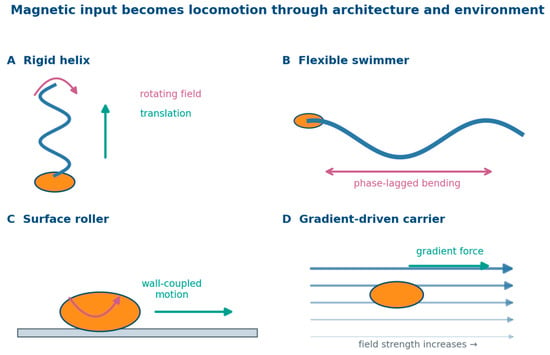
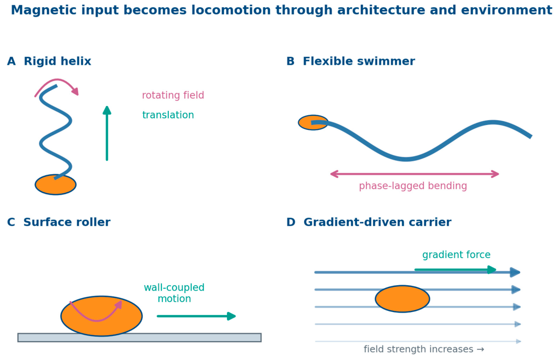
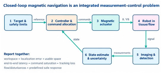
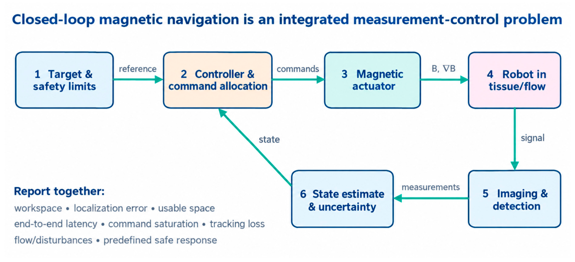
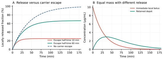
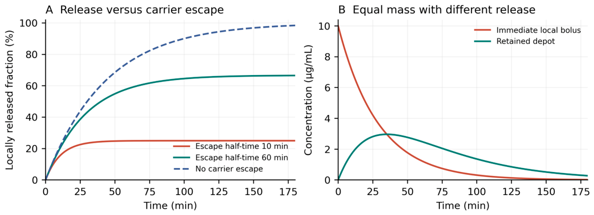
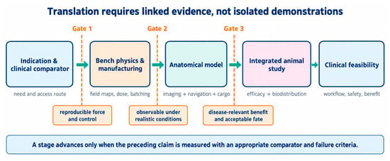
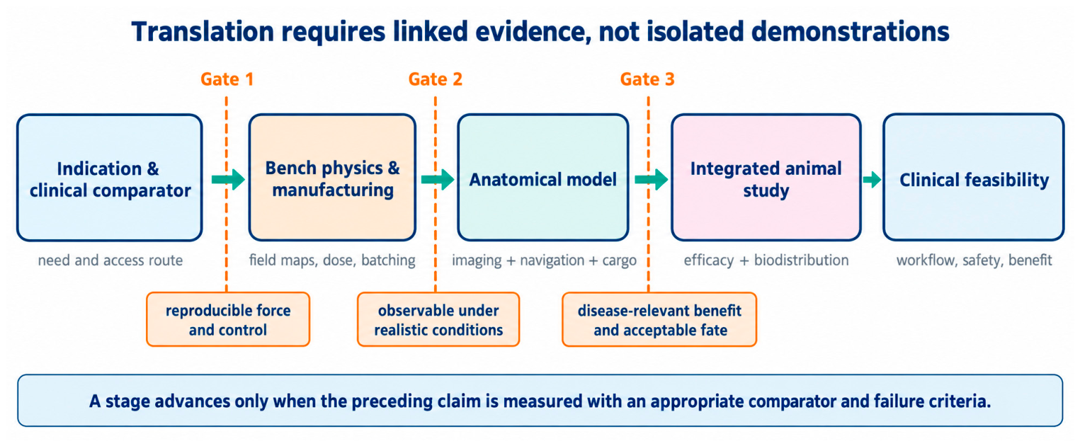

Disclaimer/Publisher’s Note: The statements, opinions and data contained in all publications are solely those of the individual author(s) and contributor(s) and not of MDPI and/or the editor(s). MDPI and/or the editor(s) disclaim responsibility for any injury to people or property resulting from any ideas, methods, instructions or products referred to in the content. |
© 2026 by the authors. Licensee MDPI, Basel, Switzerland. This article is an open access article distributed under the terms and conditions of the Creative Commons Attribution (CC BY) license.