Multi-Agent Reinforcement Learning for Emergency Medical Supply Request Regulation in Healthcare Supply Chains

Abstract

Public health emergencies place acute pressure on medical supply systems. This study develops Med-iDR-MARL, a hierarchical multi-agent reinforcement learning (MARL) framework for regulating hospital requests before allocation. Regional incentives influence hospital responses for deferrable (DD) and reducible (RD) demand, while a local scheduler retains non-deferrable (ND) demand and applies hospital-level service bounds. Across 20 simulated 30-day windows, the framework reduced DD/RD requests by 37.71% with mean incentive expenditure of CNY 274,844.23, compared with 31.03% and CNY 350,038.43 for Rule-Adaptive. Independent hospital-agent deep Q-network learning achieved greater reduction, lower expenditure, and better pooled reduction per unit expenditure. The proposed framework also had the highest peak-to-average ratio despite lower absolute peaks than No-DR. In a separate five-seed ablation, removing the minimum-service guard increased the hospital-day violation rate from zero to 58.95%. Local scheduler diagnostics found feasible solutions in 132,000 tested states but material optimality gaps and no consistent runtime advantage over vectorized exact enumeration. The results identify conditional efficiency and service trade-offs. The Shanghai COVID-19 series supplies an external risk trajectory; hospital behavior, clinical outcomes, and operational logistics remain unvalidated.

1. Introduction

Public health emergencies can rapidly transform medical supply management from routine procurement into a regional public health governance problem. During the coronavirus disease 2019 (COVID-19) pandemic, medical supplies such as masks, protective gowns, face shields, emergency equipment, intensive care unit (ICU)-related consumables, and essential medicines faced concentrated demand within a short period. The World Health Organization (WHO) emphasized the rational use of personal protective equipment (PPE) during severe shortages, with use adjusted according to care setting, activity type, and transmission risk [1]. This experience suggests that emergency supply management is not only a question of how much stock can be procured and distributed but also how demand is classified, prioritized, monitored, and coordinated across healthcare institutions.

During the pandemic, several countries and regions attempted to manage medical supply–demand through centralized platforms, consumption monitoring, and regional coordination mechanisms. For example, the United Kingdom established a PPE portal through which eligible health and social care providers could order additional COVID-19-related PPE [2]. The Centers for Disease Control and Prevention/National Institute for Occupational Safety and Health (CDC/NIOSH) provided a PPE Burn Rate Calculator to estimate PPE consumption rates, days of inventory remaining, and future ordering needs [3]. The U.S. Administration for Strategic Preparedness and Response Technical Resources, Assistance Center, and Information Exchange [4] summarized Medical Operations Coordination Centers (MOCCs) that supported hospital load balancing and regional coordination during COVID-19. These examples do not prove strategic over-requesting by hospitals; rather, they show that severe shortages made consumption monitoring, request discipline, conservation, and regional coordination operationally important. Existing tools mainly support monitoring, ordering, or allocation after requests are submitted, leaving limited mechanism-level guidance on how hospitals might adjust scheduled requests before formal allocation.

Existing studies address medical supply inventory, distribution, reallocation, and capacity decisions [5,6,7,8]. This study asks: (i) Can pre-allocation request regulation reduce pressure on regional quotas? (ii) What reduction–expenditure trade-offs arise from dynamic incentives compared with fixed incentives and hospital-only learning? (iii) How do local scheduling and minimum-service constraints affect simulated service outcomes across hospital tiers?

We develop the Medical Incentive-based Demand-Side Regulation Multi-Agent Reinforcement Learning (Med-iDR-MARL) framework. A regional coordinator sets a unit reduction incentive based on epidemic risk, supply quotas, and aggregate request pressure; hospital policies respond to local demand, delay states, and incentive signals. Local service constraints limit the resulting response before aggregate feedback informs the next regional decision.

Demand is classified as essential non-deferrable (ND), deferrable (DD), or discretionary reducible (RD). ND represents urgent care and life-sustaining supplies and is retained by the scheduler. DD represents supplies for postponable activities, whereas RD represents lower-urgency or substitutable requests that can be curtailed at a modeled dissatisfaction cost. These are simulation categories, not patient-specific clinical decisions. The Shanghai COVID-19 series is used only as an exogenous risk trajectory; hospital demands, quotas, and response parameters are representative scenarios.

In the baseline scenarios, the framework reduces schedulable requests and incentive expenditure relative to Rule-Adaptive, whereas the hospital-only learning baseline achieves stronger results on several measures. These conditional comparisons motivate three management considerations:

• At the hospital level, medical supply requests can be classified into ND, DD, and RD according to clinical necessity and operational flexibility, with consumption monitoring, request review, and delay management focused on demands with adjustment potential;
• At the regional level, coordinators can adjust coordination and incentive intensity in response to aggregate demand, supply quotas, and epidemic risk to alleviate over-quota pressure from DD and RD requests before formal allocation;
• At the governance level, ND fulfillment, minimum-guarantee compliance, differences in reduction burdens across hospitals, and incentive expenditure should be monitored jointly, rather than evaluating request regulation solely by a single reduction metric.

These considerations require evaluation with hospital requests, inventory, procurement, and response data, including institutional acceptability and implementation cost.

The remainder of the paper is organized as follows. Section 2 reviews medical supply scheduling, healthcare reinforcement learning, incentive mechanisms, and demand response. Section 3 defines the request-regulation problem and assumptions. Section 4 presents Med-iDR-MARL. Section 5 reports baseline, multi-seed, sensitivity, ablation, and safety results. Section 6 discusses implications, external validity, and limitations, and Section 7 concludes.

2. Literature Review

We position the framework against four related streams: medical supply chain optimization, healthcare reinforcement learning, incentive mechanisms, and demand response. The distinction concerns the decision being learned, the timing of that decision, and the service constraints imposed.

2.1. Medical Supply Scheduling and Emergency Supply Chains

Medical supply-chain models address inventory, capacity, routing, and distribution [6,7,8]. Recent work studies multi-period allocation under regional heterogeneity [9], pandemic purchasing strategies informed by events in the English health system [10], hospital medication-inventory MARL [11], and socially optimal PPE distributions [12]. These decision scopes complement the present model, which learns regional incentives and hospital request responses before formal allocation.

Rationing theory explains why orders may diverge from immediate consumption when scarce-capacity allocation depends on reported demand [13,14,15]. It motivates request regulation but is not evidence that hospitals falsify requests. Recent platelet inventory-distribution work addresses another related operational decision [16]. Our simulator instead generates risk-dependent baseline demand and permits request rates from zero to one; it neither identifies nor simulates strategic inflation above this baseline.

2.2. Reinforcement Learning in Healthcare Resource Management

Reinforcement learning (RL) is suitable for sequential decision problems in which current actions influence future system states. In healthcare, reinforcement learning has been applied to treatment recommendation, resource allocation, emergency response, and hospital operations. For example, ref. [17] used reinforcement learning to study treatment strategies for sepsis, while ref. [18] reviewed reinforcement learning applications in smart healthcare and emphasized long-term reward, safety constraints, and clinical interpretability. During COVID-19, collaborative reinforcement learning and agent-based methods were also explored for reallocating critical equipment, hospital beds, and staff under changing demand pressure [19,20].

Healthcare reinforcement learning includes both single-agent operational control and multi-agent coordination. Multi-agent models represent distinct institutional objectives but introduce non-stationarity and credit-assignment difficulties [21,22]. Hospital medication-inventory MARL [11] and hospital-network platelet inventory RL [23] are recent examples of supply-side decision learning. Med-iDR-MARL instead separates the regional incentive decision from each hospital’s request response and local service constraints.

2.3. Stackelberg Games and Incentive Mechanisms

Beyond healthcare reinforcement learning, this study draws on game-theoretic and incentive mechanism perspectives. Emergency medical supply requests involve interactions among regional authorities, hospitals, and other stakeholders under scarcity and incomplete information. Regional authorities are concerned with aggregate supply–demand balance, clinical safety, fiscal cost, and fairness, whereas hospitals are primarily concerned with service continuity and shortage risk. If hospital requests are treated only as fixed inputs, it is difficult to explain how incentive rules, quota pressure, and shortage expectations may affect request behavior.

Game-theoretic studies examine multi-actor public-health resource allocation. For example, ref. [24] models government, hospitals, and non-governmental public-welfare organizations in a tripartite evolutionary game. This motivates studying institutional interaction under scarcity but does not establish strategic request inflation by hospitals.

Incentive mechanism theory further suggests that managers can design rules that induce self-interested participants to make decisions closer to system-level objectives [25]. Supply chain research also shows that scarce-capacity allocation rules can shape downstream ordering behavior and system performance [14]. In healthcare, [26] proposes incentives such as service discounts and fast tracks to guide patient flows during a pandemic and improve hospital capacity utilization. These studies demonstrate the relevance of incentives in healthcare resource coordination, but they usually focus on patient choice, hospital capacity utilization, or allocation acceptance rather than hospital supply-request reduction.

The Stackelberg leader-follower structure is consistent with the management sequence studied here: the regional authority first sets a unit reduction incentive, and hospitals then respond by adjusting schedulable request rates. Traditional Stackelberg models, however, typically require explicit utility functions and follower response functions. When hospital responses depend on institutional tiers, epidemic risk, resource categories, delay pressure, and dissatisfaction costs, deriving a reliable analytical response function is difficult. Recent work on Stackelberg partially observable Markov decision processes and multi-agent reinforcement learning suggests that learning-based approximations can be used in dynamic mechanism design [27,28]. This study therefore borrows the hierarchical decision logic of Stackelberg interaction without claiming to solve a static analytical equilibrium.

2.4. Multi-Agent Reinforcement Learning and Incentive-Based Demand Response

Incentive-based demand response was developed mainly in power systems. Aggregators use prices or rewards to encourage demand-side actors to adjust consumption, relieve capacity pressure, or maintain system constraints [29,30,31]. Reinforcement learning has been used for dynamic pricing and load control [32,33], and MARL-iDR combines aggregator incentives with residential demand-side response [34]. These studies motivate the incentive–response structure but do not transfer directly to clinical supplies: emergency healthcare must protect essential demand, represent hospital tiers and delay costs, and account for minimum-service constraints. The present work adopts a finite action set for a transparent, computationally manageable simulation and a discrete local scheduler; it does not claim that discrete control is superior to continuous-policy variants such as proximal policy optimization (PPO) or deep deterministic policy gradient (DDPG).

The contribution is a coupled decision mechanism: a regional learner sets incentives, heterogeneous hospital policies adjust DD/RD requests, local service constraints limit that response, and aggregate outcomes inform the next incentive. Relative to residential incentive MARL [34], the model incorporates hospital demand categories and service floors; relative to hospital inventory RL [11,23], it addresses requests before allocation. Its novelty lies in this modeled interface and evaluation, rather than a new generic deep Q-network (DQN) architecture.

3. Problem Statement and Model Formulation

3.1. Scenario Setting and Modeling Assumptions

We consider a medical supply request-regulation system comprising a regional health authority and multiple hospitals. The authority holds a regional supply quota for deferrable and reducible resources (DD and RD) and observes the epidemic-risk index and aggregate request pressure. Each hospital observes its local demand state and dissatisfaction information, but is not required to disclose raw medical records, inventory records, or internal scheduling details. At the beginning of each decision period, the authority announces a unit reduction incentive, after which hospitals determine request rates for schedulable resources and local schedulers generate specific fulfillment plans.

The daily simulator uses representative hospital tiers and risk-driven demand. ND is retained, unserved DD incurs a delay-state penalty, and RD curtailment incurs quadratic dissatisfaction, representing increasing marginal disutility. Coefficients and service floors are illustrative assumptions. DD uses a state counter: it increments when unserved, resets after service, and also resets when it reaches MAX_DELAY = 5. Recorded states are therefore 0–4. No order-level backlog is conserved or carried into another episode, and unfinished quantities are not settled at day 30. This counter cannot establish an actual waiting-time limit. Table 1 defines the main quantities.

Table 1. Model sets, demand categories and key parameters.

Module	Symbol	Definition	Simulation Mapping or Value
Entities and indices	H	Hospital set	|H| = 20
Entities and indices	i, t, k	Hospital, daily time step and resource index	30 time steps per episode
Demand category	KDD	Set of deferrable resources	DD1 elective supplies (50); DD2 deferrable medicines (30)
Demand category	KRD	Set of reducible resources	RD1 substitutable supplies (40); RD2 non-urgent medicines (25)
Demand category	KND	Set of non-deferrable resources	ND1 emergency equipment (60); ND2 ICU supplies (35)
Demand and risk	dK	Reference demand for resource k	[DD1, DD2, RD1, RD2, ND1, ND2] = [50, 30, 40, 25, 60, 35]
Demand and risk	rt	Normalized epidemic-risk index	Read from cleaned data and clipped to [0, 1]
Demand and risk	scalei	Hospital scale factor	Tertiary 1.5; secondary 1.0; primary 0.5
Demand and risk	Bi,t,k	Baseline demand of hospital i for resource k	Bi,t,k = dk · scalei · (1 + 3rt)
Regional constraints	Dt	Regional DD and RD baseline demand	Summed across hospitals and DD/RD resources
Regional constraints	St	Regional DD and RD supply quota	St = Dt(0.85 + 0.15rt)
Decision variable	qt	Unit reduction incentive announced by the AA	{0, 1, …, 10} yuan per item
Decision variable	gi,t	PA request-rate action for DD and RD	{0.0, 0.1, …, 1.0}
Hospital parameter	αi	Minimum-service factor	Tertiary 0.8; secondary 0.7; primary 0.5
Hospital parameter	βi,k	Dissatisfaction coefficient for RD reduction	Tier-specific normal draw, clipped to [0.05, 1.50]
Evaluation metric	ηt	Regional DD and RD reduction rate	See Section 5.2
Evaluation metric	PAR	Peak-to-average ratio	See metric definition

AA denotes the aggregator agent and PA a participant agent; PAR denotes peak-to-average ratio.

At each time step, baseline demand is determined jointly by reference demand, hospital scale and epidemic risk. The notation and corresponding definitions are given below.

B_i,t,k = d_K ⋅ scale_i ⋅ (1 + 3r_t)

(1)

This formulation implies that baseline requests rise with epidemic risk and with hospital scale. Regional baseline demand for DD and RD is defined as follows.

$$D_t=\sum _{i\in H}\sum _{k\in K_{\mathit{DD}}{\cup K}_{\mathit{RD}}}{B}_{i,t,k}$$

(2)

Considering supply-chain flexibility and the risk scenario, the regional authority sets the available DD and RD supply quota at time t as follows.

S_t = D_t ⋅ (0.85 + 0.15r_t)

(3)

The quota ratio is 0.85 + 0.15r_t, where the normalized risk index r_t is clipped to [0, 1]. It therefore lies in [0.85, 1.00] without an additional lower clip. This rule provides a reproducible stress-test transition between routine and emergency conditions; it does not reproduce the quota mechanism of a particular region.

3.2. Hospital Heterogeneity and Medical Supply–Demand Categories

Hospitals at different tiers differ systematically in clinical responsibilities, service catchment areas and resource-consumption intensity during public health emergencies. Tertiary hospitals commonly undertake a larger share of critical care and regional referral, secondary hospitals provide routine care and part of emergency care, and primary hospitals mainly provide community screening, transfer, and basic services. Their baseline demand, minimum-service requirements and sensitivity to request reductions therefore differ. Treating all hospitals as homogeneous would obscure demand differences in a tiered delivery system and could mask distributional effects of incentives.

The scenario distinguishes tertiary, secondary, and primary hospitals through scale, minimum-service factors, and dissatisfaction coefficients (Table 2). Higher values for tertiary hospitals express an assumed combination of greater referral responsibility and service rigidity. These numerical settings are representative modeling choices, not estimates of hospital preferences or calibrated clinical thresholds.

Table 2. Tier-specific scenario parameters and response settings.

Hospital Tier	Hospitals	Scale Factor Scalei	Minimum-Service αi	Mean RD Dissatisfaction βi	SD of βi	Scenario Interpretation
Tertiary	10	1.5	0.8	0.70	0.05	Greater regional referral and critical-care responsibility; stronger service rigidity
Secondary	8	1.0	0.7	0.50	0.08	Routine care and part of emergency and critical care
Primary	2	0.5	0.5	0.30	0.10	Community-oriented services with relatively greater adjustment flexibility

The hospital-level RD dissatisfaction coefficient is drawn from tier-specific normal distributions: N(0.70, 0.05²), N(0.50, 0.08²), and N(0.30, 0.10²) for tertiary, secondary, and primary hospitals, respectively. The implementation adds resource-level normal perturbations with standard deviation (SD) 0.02 and clips the resulting coefficients to [0.05, 1.50]. These coefficients multiply RD reduction costs; DD delay penalties are modeled separately. The settings express a service-rigidity hypothesis and are examined through sensitivity analysis, not estimated from hospital preferences.

Because hospital-level daily request and inventory data are unavailable, the study does not seek point predictions of consumption at any specific hospital. Instead, it uses representative scenario parameterization, translating hospital tier structure, epidemic-risk trajectories, and evidence on peak medical-resource demand into controllable simulation inputs. The results therefore assess the mechanism and relative performance of Med-iDR-MARL rather than provide a complete empirical reconstruction of a city-level medical supply chain.

The six representative resource proxies are DD1 (elective supplies), DD2 (deferrable medicines), RD1 (substitutable supplies), RD2 (non-urgent medicines), ND1 (emergency equipment), and ND2 (ICU supplies). They describe operational flexibility in the simulation, not a universal clinical inventory taxonomy. ND is retained; DD service updates the delay-state counter; RD service is chosen from 11 discrete fractions.

Each hospital’s total request comprises ND, DD, and RD. Its participant agent (PA) chooses a DD/RD request rate. The dynamic constrained knapsack scheduler (DCKP) retains ND and seeks a schedule within the hospital-level service interval. This aggregate constraint does not impose a separate floor for every resource or patient group.

3.3. Hierarchical Interaction Between the Regional Authority and Hospitals

We model regional medical supply request regulation as a hierarchical interaction between a regional health authority and multiple hospitals. The authority is represented by an aggregator agent (AA), which determines a unit reduction incentive from regional demand pressure, supply quota, and epidemic risk. Hospitals are represented by participant agents (PAs), which choose request rates for schedulable resources using local demand states, tier-specific parameters, delay pressure and the incentive signal. This sequence mirrors a leader-follower management process in which the authority announces an incentive rule before hospitals adjust their requests.

The AA observes regional demand, quota, risk, and incentive history; each PA uses local demand and delay-state information. Raw hospital records need not enter the AA’s state. Formal privacy and governance implications are discussed in Section 6.2.

At each time step, the epidemic-risk index determines baseline demand and the regional supply quota, thereby generating current supply–demand pressure. The AA then selects a unit reduction incentive from the aggregate state. Each PA observes the incentive and its local state and chooses a response for DD and RD. The local DCKP subsequently prioritizes ND and applies the minimum-service constraint to determine fulfillment of DD and RD. The environment calculates AA and PA rewards from realized requests, reductions, dissatisfaction, incentive expenditure, and regional supply–demand pressure and then updates the state for the next step.

Unlike a supply-side allocation model, the AA does not determine how much supply each hospital receives. It influences hospitals’ willingness to request schedulable resources through the incentive rate. At low incentives, hospitals may retain high request intensity to reduce their own shortage risk; at higher incentives, they may voluntarily reduce portions of DD or RD in exchange for compensation. The authority can therefore relieve regional pressure from the demand side without intervening in hospitals’ internal resource decisions.

Incentives apply only to DD/RD. ND is retained by construction and is outside the regional schedulable-demand quota. Consequently, full modeled ND fulfillment means that the request-regulation mechanism does not curtail ND; it is not evidence that a physically constrained supply network could deliver all urgent supplies.

The PA request rate sets a preferred DD/RD ceiling, raised when necessary to respect the minimum-service floor. DCKP approximates the following local cost-minimization problem over binary DD service choices and eleven RD service fractions.

$$\mathit{min}\sum _j{c}_{j,t}^{\mathit{DD}}\left(1-x_{j,t}^{\mathit{DD}}\right)+\sum _j{\beta }_{i,j}{\left(1-z_{j,t}^{\mathit{RD}}\right)}^2$$

(4)

The constraints include the request-rate ceiling and the lower bound imposed by the minimum-service requirement.

$$E_{i,t}^{\mathit{ND}}+{\sum }_j{x}_{j,t}^{\mathit{DD}}{d}_{j,t}^{\mathit{DD}}+{\sum }_j{z}_{j,t}^{\mathit{RD}}{d}_{j,t}^{\mathit{RD}}\le {\mathit{L}}_{i,t}$$

(5)

$$E_{i,t}^{\mathit{ND}}+{\sum }_j{x}_{j,t}^{\mathit{DD}}{d}_{j,t}^{\mathit{DD}}+{\sum }_j{z}_{j,t}^{\mathit{RD}}{d}_{j,t}^{\mathit{RD}}\ge {\alpha }_i{B}_{i,t}$$

(6)

Here, the DD cost is ((delay + 1)/5)² and each RD term is weighted by its dissatisfaction coefficient. The total service interval is defined by ND demand, the PA request-rate action, and the hospital-level minimum-service factor α_i. A greedy schedule is used when feasible; a finite-grid search repairs interval violations.

$$L_{i,t}={\mathit{E}}_{i,t}^{\mathit{ND}}+\mathit{max}\left(g_{i,t}{D}_{i,t}^{\mathit{DD}+\mathit{RD}},\hspace{1em}{\alpha }_i{B}_{i,t}-E_{i,t}^{\mathit{ND}},\hspace{1em}0\right)$$

(7)

The AA and PA are formulated as coupled Markov decision processes. The AA MDP learns regional dynamic incentives, whereas the PA MDP represents hospital request responses conditional on local states and incentives. They are connected through incentive rates, realized requests and system feedback, forming the decision framework of Med-iDR-MARL.

3.4. MDP Formulation and Reward Design

3.4.1. State, Action and Reward of the AA

The AA represents the regional health authority. At each time step, it selects a unit reduction incentive from regional supply–demand pressure, epidemic risk, and the previous incentive level to encourage reductions in DD and RD requests. It operates on aggregate rather than hospital-level clinical, inventory or scheduling information.

The state space of the AA is defined as a four-dimensional vector.

$$s_t^A=\left({\displaystyle \frac{D_t}{D_{\mathit{max}}}},\hspace{1em}{\displaystyle \frac{S_t}{D_t}},\hspace{1em}{r}_t,\hspace{1em}{\displaystyle \frac{q_{t-1}}{q_{\mathit{max}}}}\right)$$

(8)

The components represent regional DD and RD baseline demand normalized by a demand constant, the available regional supply quota, the normalized epidemic-risk index and the normalized incentive rate in the previous period. Together, they allow the AA to assess quota tightness, current risk and its own recent incentive decisions.

The action space of the AA is a discrete set of incentive rates.

$$a_t^A \in \{0,1, \dots ,10\}, q_t=a_t^A$$

(9)

The action denotes the unit incentive for reducing schedulable demand. To prevent abrupt changes between adjacent time steps, a smoothing constraint is imposed on incentive-rate variation.

q_t ← clip(q_t, q_t−1 − Δ_max, q_t−1 + Δ_max), Δ_max = 3

(10)

$$\begin{array}{c}{R}_t^A=\left(1-r_t\right)U_t+{\mathit{r}}_t{w}_r{\eta }_t-\rho \cdot {\mathit{surplus}}_t^{1.5}\left(1+r_t\right)\\ -w_c{\psi }_t{C}_t-w_p{P}_t-w_s{\displaystyle \frac{\left|q_{\mathit{t}}-q_{t-1}\right|}{q_{\mathit{max}}}}\end{array}$$

(11)

The AA reward combines within-quota utilization, DD/RD reduction, over-quota pressure, normalized incentive expenditure, an exponentially weighted peak penalty, and incentive changes. The configuration uses w_r = 1.0, ρ = 1.5, w_c = 0.15, w_p = 0.5, w_s = 0.05, and an exponential-mean coefficient of 0.3. The peak penalty is a daily excess-over-running-mean proxy, not a direct optimization of episode PAR.

This reward design balances quota utilization and cost control at low risk, while placing greater emphasis on schedulable-demand reduction and over-quota control at high risk. The incentive-cost and smoothing terms discourage excessive or volatile incentives.

AA state transitions depend on PA request responses, DCKP scheduling outcomes, the evolution of DD delay states, and epidemic risk in the next period. The AA maximizes the following discounted cumulative reward.

$$\mathit{max}\mathbb{E}\left[{\displaystyle \sum _{t=0}^{T-1}}{\left({\gamma }_A\right)}^t{R}_t^A\right]$$

(12)

The discount factor of the AA is specified in the experimental configuration.

3.4.2. State, Action and Reward of the PA

Each PA represents one hospital. After observing its local state and the AA incentive, it selects a request rate for DD and for RD. Each hospital has an Independent DQN to learn a differentiated response policy under varying delay pressure, non-deferrable demand and incentive intensity. PAs neither observe the detailed states of other hospitals nor directly access aggregate regional supply–demand information.

The local observation of hospital i at time t is represented by an eight-dimensional vector.

$$s_{i,t}^P=\left({\tilde{d}}_{i,t}^{\mathit{DD}1},{\tilde{d}}_{i,t}^{\mathit{DD}2},{\tilde{z}}_{i,t-1}^{\mathit{RD}1},{\tilde{z}}_{i,t-1}^{\mathit{RD}2},{\tilde{n}}_{i,t}^{\mathit{ND}1},{\tilde{n}}_{i,t}^{\mathit{ND}2},{\tilde{B}}_{i,t},{\displaystyle \frac{q_t}{q_{\mathit{max}}}}\right)$$

(13)

The state includes normalized delay states for two DD categories, fulfillment levels for two RD categories in the previous period, levels of two ND categories, the hospital’s normalized baseline demand, and the normalized incentive announced by the AA. It therefore captures local delay pressure, clinical rigidity, demand scale and the external incentive signal.

The PA action is a discrete request-rate choice.

g_i,t ∈ {0.0, 0.1, …, 1.0}

(14)

A value of one corresponds to full requests for DD and RD baseline demand; lower values represent stronger voluntary compression of schedulable demand in response to incentives. The PA action does not reduce ND. ND is incorporated first in DCKP scheduling so that rigid clinical demand is not crowded out by reductions in schedulable demand.

The PA reward represents the trade-off among incentive income, demand reduction, and service dissatisfaction.

$$R_{i,t}^P={\displaystyle \frac{q_t}{q_{\mathit{max}}}}\cdot {\eta }_{i,t}\cdot {\gamma }_{i,t}-{\mathit{Diss}}_{i,t}$$

(15)

The first term denotes the hospital-level reduction relative to DD and RD baseline demand, and the delay penalty factor is defined as follows.

$${\gamma }_{i,t}=1 -{\displaystyle \frac{\mathit{max}({\mathit{delay}}_{i,t}^{\mathit{DD}})}{\mathit{MAX}\_\mathit{DELAY} - 1}}$$

(16)

The delay factor reduces the incentive-related reward when the DD state counter is high; the separate normalized dissatisfaction term penalizes unserved DD and RD curtailments. These terms encourage modeled service continuity but do not impose an order-level delivery deadline.

PA state transitions depend on local DD counters, previous RD fulfillment, current ND demand, baseline demand, and subsequent incentive signals. Each PA maximizes its discounted cumulative reward using the request-rate set in Equation (13).

$$\mathit{max}\mathbb{E}\left[{\sum }_{t=0}^{T-1}({\gamma }_P{)}^t{R}_{i,t}^P\right]$$

(17)

The PA discount factor is specified in the experimental configuration. This MDP allows a hospital to adjust schedulable requests autonomously while retaining priority protection for ND through DCKP constraints.

3.4.3. Joint Training Objective Under Hierarchical Interaction

AA and PA have distinct state spaces, action spaces and reward functions, but they are not Independent. The incentive selected by the AA enters each PA observation and shapes DD and RD request rates. After DCKP scheduling, PA responses determine realized schedulable consumption, reductions and dissatisfaction, which in turn affect the regional reward received by the AA. The agents are therefore coupled through an incentive–response–scheduling feedback loop.

Within each period, the environment generates demand and quota; the AA announces an incentive; each PA chooses a request rate; the local scheduler retains ND and seeks fulfillment within the service interval; and realized requests, delay, dissatisfaction, and expenditure determine rewards and subsequent states.

The AA and PA have different but coupled objectives. The AA seeks to reduce regional schedulable demand while maintaining quota utilization and controlling incentive expenditure.

$$\underset{{\pi }_A}{\mathit{max}}E\left[{\sum }_{t=0}^{T-1}({\gamma }_A{)}^t{R}_t^A\right]$$

(18)

Each PA instead balances individual incentive income against service dissatisfaction.

$$\underset{{\pi }_i^P}{\mathit{max}}E\left[{\sum }_{t=0}^{T-1}({\gamma }_P{)}^t{R}_{i,t}^P\right]$$

(19)

The corresponding policies are the AA incentive policy and the request-response policy of hospital i. Their objectives are not identical: the AA seeks regional demand compression at controlled cost, whereas each PA balances compensation against service continuity. This difference motivates hierarchical multi-agent reinforcement learning rather than a single-agent model or a fixed response function.

AAs and PAs have Independent DQNs and replay buffers. Training alternates between AA updates and PA updates in blocks of 10 episodes, with network updates restricted to the active side. The coupled incentive–response process remains non-stationary across blocks; alternation does not establish convergence to a Stackelberg equilibrium.

The AA and PAs use 11 evenly spaced discrete actions. This finite set keeps the DQN output layer small, gives the incentive and request-rate choices directly interpretable increments, and aligns PA actions with the scheduler’s discrete fulfillment levels. Continuous-policy PPO or DDPG could represent finer changes but would require a different action parameterization and constraint treatment; their comparative performance is left for future work.

4. Med-iDR-MARL Algorithm

4.1. Overall Framework

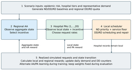
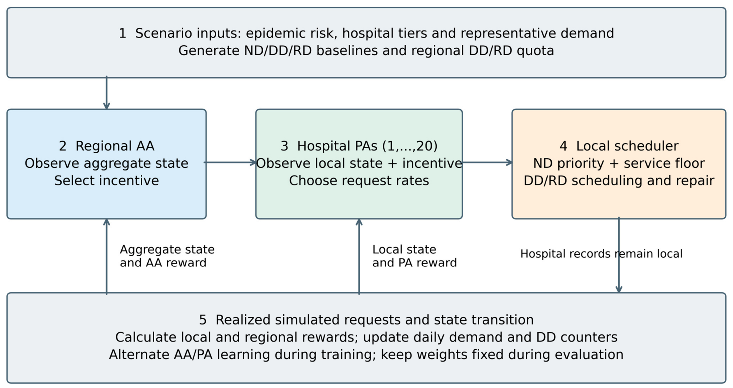
Med-iDR-MARL links a regional incentive policy to local hospital response policies through constrained scheduling and aggregate feedback (Figure 1).

Figure 1. Med-iDR-MARL components and within-period sequence.

The framework contains an AA, hospital-level PAs and a local DCKP scheduler. The AA represents the regional health authority and selects a unit reduction incentive from regional DD and RD pressure, supply quota, epidemic risk, and the preceding incentive level. Each PA represents a hospital and chooses a schedulable request rate using local delay states, non-deferrable demand, baseline demand and the incentive signal. The DCKP translates the PA request rate into resource-specific DD and RD fulfillment while prioritizing ND and the minimum-service constraint.

Figure 1 shows the daily decision sequence. Local observations and rewards support PA transitions, while aggregate outcomes support the AA transition. During training, network updates alternate between AA and PAs, and during evaluation, weights remain fixed.

Unlike supply-side scheduling methods that directly assign inventory, Med-iDR-MARL learns an aggregate incentive intended to influence only schedulable DD and RD requests. It is a simulated demand-preprocessing module that precedes replenishment, formal allocation, and distribution; it is not a replacement for clinical decisions or operational logistics.

4.2. AA Policy Learning

The AA uses DQN to learn a regional dynamic incentive policy. Its input is the four-dimensional aggregate state, and its output is the Q value for each of 11 discrete incentive actions. The action set is {0, 1, …, 10}, representing unit reduction incentives. The network consists of an input layer, two hidden layers with 64 ReLU units each, and an 11-dimensional output layer.

The AA uses epsilon-greedy exploration during training, decreasing epsilon from 1.0 to 0.10. Its soft-top3 option samples among high-valued actions when Q values are close. Evaluation sets epsilon to zero but retains this sampling unless the soft-top3 component is ablated; therefore, a fixed checkpoint alone does not make evaluation deterministic.

AA DQN updates use experience replay. After each action, the state, action, reward, next state and terminal indicator are stored in a replay buffer, from which mini-batches are sampled for optimization.

For a sampled transition, the AA target Q value is defined as follows.

$$y_t^A=R_t^A+{\mathit{\gamma }}_A\underset{\mathit{a’}}{\mathit{max}}{Q}_A^{-}\left(s_{t+1}^A,\mathit{a’}\right)$$

(20)

The target network and AA discount factor are used to compute the target. The online network is updated by minimizing the following mean-squared error.

$$L_A=\mathbb{E}\left[{\left(y_t^A-Q_A(s_t^A,a_t^A)\right)}^2\right]$$

(21)

To improve training stability, the AA uses an Independent target network that is synchronized through soft updates.

$${\theta }_A^{-}\leftarrow \tau {\theta }_A+(1-\tau ){\theta }_A^{-}$$

(22)

The parameters denote those of the online and target networks, respectively, with τ = 0.005. This update mitigates instability caused by rapidly changing targets.

4.3. PA Policy Learning

Each PA represents one hospital and has an Independent DQN to learn a heterogeneous request-response policy. The input is an eight-dimensional local observation, comprising delay states of two DD categories, fulfillment levels of two RD categories in the preceding period, levels of two ND categories, baseline demand and the normalized AA incentive. The output is the Q value for each of 11 discrete request-rate actions.

The PA uses the request-rate action set defined in Equation (13); the resulting requests are processed by DCKP, as described in Section 4.4.

The PA network mirrors the AA architecture, with an input layer, two 64-unit ReLU hidden layers and an 11-dimensional linear output layer. Each PA has an Independent replay buffer and Q network, enabling policies to adapt to hospital tier, demand scale, delay pressure, and dissatisfaction sensitivity.

$$y_{i,t}^P=R_{i,t}^P+{\gamma }_P\underset{a\prime }{\mathit{max}}{Q}_i^{P-}(s_{i,t+1}^P,a\prime )$$

(23)

The target network of hospital i and the PA discount factor define the target value. The PA updates the online network by minimizing the following loss.

$$L_i^P=E\left[{\left(y_{i,t}^P-Q_i^P\left(s_{i,t}^P,a_{i,t}^P\right)\right)}^2\right]$$

(24)

The PA reward jointly considers incentive income, reduction, DD delay cost, and RD dissatisfaction cost. Hospitals therefore balance compensation against service continuity rather than pursue reductions alone. Independent DQNs allow hospitals at different tiers to develop differentiated request policies.

4.4. DCKP Constrained Scheduler

This section describes the implementation and role of DCKP, building on the formal definition and rules in Section 3.3.

DCKP converts the PA request rate into resource-specific fulfillment. It first serves DD in descending delay-cost order, allocates the remaining budget to discrete RD levels, and attempts to complete any minimum-service deficit. The audited implementation additionally checks the resulting total against the lower and upper bounds and uses finite-grid repair when it lies outside that interval. This repair is a substantive part of the evaluated implementation; the original description did not specify it. A versioned historical source snapshot was not retained, so its original introduction date and use in each earlier training cohort cannot be established.

For lower bound L = α_iB_i,t and upper bound U = max(ND demand, request ceiling), repair is triggered when realized total E < L − 10⁻⁸ or E > U + 10⁻⁸. It enumerates 2² × 11² = 484 DD/RD combinations and selects the first minimum-cost feasible candidate in enumeration order. If no candidate is feasible, the implementation retains the pre-repair schedule; the diagnostic records infeasibility. An ND-only early return occurs when ND reaches U. Thus, feasibility must be checked for the actual state rather than assumed for every possible input.

DCKP receives DD demand and delay states, RD demand and dissatisfaction coefficients, ND demand, the PA request-rate ceiling, and the hospital minimum-service factor. It outputs DD fulfillment, RD service levels, realized consumption, and dissatisfaction cost. Its local performance is compared with exhaustive enumeration over the same action grid in Section 5.

4.5. Training Procedure and Experimental Extensions

Each episode consists of 30 daily steps, and training runs for 8000 episodes. AA-side and PA-side updates alternate in 10-episode blocks, beginning with the AA. Within each block, only the active side stores transitions and updates its networks; the inactive side acts with ε = 0 while its weights remain fixed. Target networks on the active side are soft-updated at each time step with τ = 0.005, whereas all target networks are hard-synchronized every 50 episodes. The stored AA and PA exploration rates are multiplied by 0.999 at the start of each episode, subject to a minimum of 0.10. The normalized Shanghai risk sequence drives simulated demand and quota variation; it does not reconstruct hospital scheduling in Shanghai.

Algorithm 1 summarizes the Med-iDR-MARL training procedure.

Algorithm 1: Med-iDR-MARL Training Procedure

Input: Hospital set H, resource set K, epidemic-risk series {rt}, number of training episodes N, episode length T, tier-specific parameter settings, and DQN hyperparameters         Output: Trained AA incentive policy πA and PA DD/RD request-rate policy πiP for each hospital i ∈ H         Initialize the AA online Q-network QA, target network QA−, and replay buffer; 1.   for each hospital i ∈ H, initialize the PA online Q-network QiP, target network QiP−, and replay buffer; 2.   Assign scalei and αi by hospital tier and sample βi,k from the corresponding tier-specific distribution; 3.   Set active ← AA; 4.   for episode = 1, …, N do 5.   Reset the environment, sample a length-T window from {rt}, and generate simulated demands and regional DD/RD quotas; 6.   Decay the stored AA and PA exploration rates: ε ← max(0.10, 0.999ε); 7.   if (episode − 1) mod 50 = 0 then 8.   Hard-synchronize all target networks with their corresponding online networks; 9.   end if 10. for t = 1, …, T do 11. AA observes stA and selects the unit reduction incentive qt, using its stored ε only when the AA is active; 12. for each hospital i ∈ H do 13. PAi observes si,tP and selects the DD/RD request rate gi,t, using its stored ε only when the PAs are active; 14. DCKP computes DD/RD fulfillment under ND priority and the minimum-service constraint; 15. Compute the PA reward Ri,tP and advance the hospital state; 16. end for 17. Aggregate realized regional DD/RD requests, request reduction, incentive expenditure, and over-quota pressure; 18. Compute the AA reward RtA and advance the regional state; 19. Store completed transitions for the active side; once the relevant replay buffer contains at least 64 samples, draw a mini-batch and update the active online network(s), while holding the other side fixed; 20. Soft-update only the active target network(s) with τ = 0.005; 21. end for 22. Store the terminal transition for the active learning side; 23. if episode mod 10 = 0 then 24. Switch the active learning side between the AA and the PAs; 25. end if 26. end for

5. Simulation Experiments and Results

5.1. Data and Experimental Environment

We used cleaned daily COVID-19 data from Shanghai to construct the epidemic-risk sequence from 22 January 2020 to 8 January 2023 (1079 observations). The normalized risk index was clipped to [0, 1] and used as an external dynamic pressure source for baseline demand and regional supply quotas. The Shanghai data were used solely to construct an external risk-shock trajectory and do not imply that the simulation reproduces the Shanghai hospital system.

The representative network has 10 tertiary, 8 secondary, and 2 primary hospitals. Tier counts, scale factors, and service thresholds are scenario settings (Table 2) rather than an exact reconstruction of hospital counts or bed shares in a particular city.

The reference-demand vector is [DD1, DD2, RD1, RD2, ND1, ND2] = [50, 30, 40, 25, 60, 35] items. Hospital scale and the factor 1 + 3r_t determine baseline demand; the latter permits a fourfold stress level at r_t = 1 and is not a fitted estimate of consumption or strategic inflation. The regional quota applies only to DD/RD. The six resource labels are representative proxies.

All baseline methods pass their request actions through the current scheduler, including No-DR at request rate one. ND is retained and the hospital service floor is enforced when a feasible local grid point exists. Discrete scheduling can therefore produce a small reduction even for No-DR. These outcomes describe regulated simulated requests, not physical deliveries.

Both AA and PAs use two 64-unit hidden layers, learning rate 0.0005, batch size 64, and replay capacity 50,000; discount factors are 0.95 and 0.90. Table 3 re-evaluates the stored MARL and Independent policies without retraining. The baseline audit used Python 3.12.4, TensorFlow 2.20.0, and NumPy 2.3.4 on Windows CPU, with oneDNN disabled and one intra-/inter-operation thread. Python, NumPy, and TensorFlow seeds were set to 2026 before environment and network construction. Test epsilon was zero, AA soft-top3 remained active, and the original loading and evaluation order was preserved. Three Independent processes reproduced the supplied result file exactly.

Table 3. Baseline performance across 20 test scenarios (mean ± SD).

Metric	No-DR	Rule-Fixed	Rule-Adaptive	Med-iDR-MARL	Independent-PA-DQN
PAR	1.6502 ± 0.2989	1.6450 ± 0.2961	1.6443 ± 0.2960	1.7038 ± 0.3153	1.6692 ± 0.2906
P95 daily DD/RD requests (items)	11,714.60 ± 2693.54	9386.86 ± 2148.60	8106.13 ± 1847.50	7406.74 ± 1678.01	7301.21 ± 1711.32
Mean absolute daily peak (items)	12,047.39 ± 2461.11	9648.57 ± 1965.55	8326.95 ± 1689.14	7797.10 ± 1619.49	7564.13 ± 1548.98
DD/RD reduction rate	0.0059 ± 0.0015	0.2014 ± 0.0007	0.3103 ± 0.0000	0.3771 ± 0.0057	0.3836 ± 0.0011
Mean scenario ROI (items/CNY)	N/A	0.3333 ± 0.0000	0.2000 ± 0.0000	0.3889 ± 0.1382	0.3333 ± 0.0000
Mean scenario incentive expenditure (CNY)	0.00 ± 0.00	136,199.31 ± 35,060.21	350,038.43 ± 90,838.82	274,844.23 ± 164,943.34	259,768.38 ± 68,025.20
Over-quota requests (items/scenario)	14,365.38 ± 3047.32	0.00 ± 0.00	0.00 ± 0.00	0.00 ± 0.00	0.00 ± 0.00
Mean incentive (CNY/item)	0.0000 ± 0.0000	3.0000 ± 0.0000	5.0000 ± 0.0000	2.6417 ± 0.8037	3.0000 ± 0.0000
ND fulfillment rate	1.0000 ± 0.0000	1.0000 ± 0.0000	1.0000 ± 0.0000	1.0000 ± 0.0000	1.0000 ± 0.0000
Mean bounded DD counter	0.0000 ± 0.0000	0.0000 ± 0.0000	0.0000 ± 0.0000	0.7318 ± 0.0226	0.6128 ± 0.0137
Maximum bounded DD counter	0.0000 ± 0.0000	0.0000 ± 0.0000	0.0000 ± 0.0000	4.0000 ± 0.0000	4.0000 ± 0.0000
Normalized RD dissatisfaction	0.0000 ± 0.0000	0.0017 ± 0.0004	0.0021 ± 0.0006	0.0009 ± 0.0002	0.0011 ± 0.0003
Minimum-service violation rate	0.0000 ± 0.0000	0.0000 ± 0.0000	0.0000 ± 0.0000	0.0000 ± 0.0000	0.0000 ± 0.0000
Pooled ROI (items/CNY)	N/A	0.3333	0.2000	0.3094	0.3333

Note: Means and descriptive SDs use the 20 fixed test scenarios (SD denominator n = 20, consistent with the supplied baseline export); these are not confidence intervals. Pooled ROI is a single ratio across all scenarios and has no scenario SD. Costs and over-quota quantities are per 30-day scenario. DD metrics describe the bounded state counter. Normalized RD dissatisfaction divides accumulated quadratic RD-curtailment cost by baseline DD/RD demand. Values displayed as 0.0000 may reflect rounding.

All five baseline methods use the same test beta matrix. Loading hospital checkpoints restores these coefficients into the shared environment; because Independent is loaded after MARL, the common matrix is the one saved with Independent. It differs from the MARL-saved matrix by at most 0.21744. This is a common-environment comparison of stored policies, but not a comparison with matched training coefficients. The Independent summary records seed 0 and 8000 episodes; the original MARL training seed, execution version, and checkpoint-selection history are not completely traceable. No checkpoint was selected using the present audit results.

All evaluation windows start at indices 30, 35, …, 125 and last 30 days. The windows overlap. The current training code samples start from the same risk series without excluding these dates, so evaluation is not a held-out temporal generalization test. Table 4 summarizes earlier 10-seed training traces; Table 5 retains earlier beta-condition summaries. Their execution versions are not bound to archived source hashes, and neither was rerun in this audit. Table 6 and Table 7 use a separate five-seed ablation with completed 8000-episode training logs. These cohorts therefore cannot be interpreted as repeated evaluations of one authenticated training implementation.

Table 4. Late-stage training statistics across random seeds.

Metric	Mean ± Sample SD	Minimum	Maximum
PAR	1.3400 ± 0.0370	1.2984	1.3916
AA reward	13.9114 ± 0.3289	13.3754	14.3752
DD/RD reduction rate	0.3303 ± 0.0217	0.3049	0.3609
Zero-incentive proportion	0.2934 ± 0.1781	0.0096	0.4633

Note: Table 4 reports the sample SD of 10 seed-level late-training averages (denominator n − 1). The zero-incentive proportion is the fraction of daily steps with q_t = 0. Historical ROI fields are not used here because their zero-cost episode convention cannot be reconstructed from the retained summaries.

Table 5. Sensitivity analysis of the beta coefficient.

Beta Multiplier	DD/RD Reduction	Mean Scenario Expenditure (CNY)	Mean Incentive (CNY/Item)	Seeds × Scenarios
β × 0.8	0.3445 ± 0.0252	218,261.18 ± 64,577.58	1.9807 ± 0.7958	10 × 20
β × 1.0	0.3402 ± 0.0221	218,636.48 ± 48,207.22	1.8708 ± 0.4710	10 × 20
β × 1.2	0.3514 ± 0.0197	255,778.21 ± 74,011.00	2.4757 ± 0.9459	10 × 20

Note: Mean ± sample SD across 10 seed-level scenario averages. This cohort precedes the five-seed repaired-scheduler ablation. Comparisons are within Table 5; its β × 1.0 condition is not the full-model cohort of Table 6.

Table 6. Efficiency and regional-pressure ablation results across five seeds (mean ± SD).

Variant	DD/RD Reduction	PAR	Within-Seed Pooled ROI (Items/CNY)	Mean Scenario Cost (CNY)	Mean Incentive (CNY/Item)	Over-Quota Requests
Full	0.3093 ± 0.0361	1.6348 ± 0.0843	0.6833 ± 0.5942	162,469.40 ± 102,395.13	1.3533 ± 0.7223	0.00 ± 0.00
w/o DCKP	0.3065 ± 0.0255	1.6256 ± 0.0717	0.4781 ± 0.1234	153,329.76 ± 27,706.59	1.1337 ± 0.1486	0.00 ± 0.00
w/o risk	0.3319 ± 0.0174	1.7320 ± 0.0864	0.4502 ± 0.0913	172,991.86 ± 35,078.06	1.5950 ± 0.2793	0.00 ± 0.00
w/o heterogeneity	0.4087 ± 0.0378	1.7066 ± 0.1090	0.4886 ± 0.1377	169,113.83 ± 53,359.69	1.5587 ± 0.6957	0.00 ± 0.00
w/o smoothing	0.3264 ± 0.0433	1.6758 ± 0.0545	0.4578 ± 0.1250	172,401.35 ± 49,299.90	1.5610 ± 0.6182	0.00 ± 0.00
w/o soft-top3	0.3211 ± 0.0419	1.6242 ± 0.0736	0.4480 ± 0.3176	221,444.78 ± 136,014.18	2.0620 ± 1.7750	0.00 ± 0.00
w/o min-service guard	0.6130 ± 0.0455	2.3604 ± 0.3404	0.5074 ± 0.1328	294,940.83 ± 81,801.91	1.2013 ± 0.4027	0.00 ± 0.00

Note: Mean ± sample SD across five training seeds (denominator n − 1), with 20 scenario averages per seed. Within-seed pooled ROI weights scenarios by expenditure; the table then gives each seed equal weight. It is not the ratio obtained by pooling all five seeds together. Table 3 uses a different fixed checkpoint and scenario-level dispersion. These descriptive comparisons do not establish statistical superiority.

Table 7. Hospital-day service summaries from the completed rerun across five training seeds (mean ± sample SD).

Variant	ND Fulfillment (%)	Mean Bounded DD Counter	Normalized RD Cost	Violation Rate (%)	Tier 3 (%)	Tier 2 (%)	Tier 1 (%)
Full	100.00 ± 0.00	0.3112 ± 0.0256	0.0011 ± 0.0004	0.00 ± 0.00	0.00 ± 0.00	0.00 ± 0.00	0.00 ± 0.00
w/o DCKP	100.00 ± 0.00	0.1772 ± 0.0669	0.0013 ± 0.0002	0.00 ± 0.00	0.00 ± 0.00	0.00 ± 0.00	0.00 ± 0.00
w/o risk	100.00 ± 0.00	0.3035 ± 0.0225	0.0012 ± 0.0001	0.00 ± 0.00	0.00 ± 0.00	0.00 ± 0.00	0.00 ± 0.00
w/o heterogeneity	100.00 ± 0.00	0.3286 ± 0.0486	0.0012 ± 0.0003	0.00 ± 0.00	0.00 ± 0.00	0.00 ± 0.00	0.00 ± 0.00
w/o smoothing	100.00 ± 0.00	0.2854 ± 0.0321	0.0013 ± 0.0003	0.00 ± 0.00	0.00 ± 0.00	0.00 ± 0.00	0.00 ± 0.00
w/o soft-top3	100.00 ± 0.00	0.2938 ± 0.0691	0.0012 ± 0.0005	0.00 ± 0.00	0.00 ± 0.00	0.00 ± 0.00	0.00 ± 0.00
w/o min-service guard	100.00 ± 0.00	0.6422 ± 0.0981	0.0022 ± 0.0002	58.95 ± 3.03	66.39 ± 5.35	54.68 ± 3.51	38.78 ± 12.57

Note: Each seed first averages 20 scenarios; dispersion is the sample SD across five seeds. One violation is E_i,t + 10⁻⁸ < α_i B_i,t, with 600 hospital-days per scenario and tier denominators of 300, 240, and 60. Removing the guard produced 353.69 ± 18.20 violating hospital-days per scenario. Overall rates use hospital-count weights 10:8:2. DD is a bounded state counter. Saved seed summaries were rounded before aggregation; original hospital-day records are unavailable. The homogeneous variant changes tiers and service floors, so its tier columns are not a like-for-like fairness comparison.

5.2. Baseline Comparison and Overall Performance

The four baselines are No-DR (q = 0, request rate 1), Rule-Fixed (q = 3 CNY/item, request rate 0.8 whenever q > 0), Rule-Adaptive, and Independent-PA-DQN (learned hospital policies under q = 3, without a learned AA). Rule-Adaptive selects q = 5 when the quota-to-baseline ratio is below 1.05 and otherwise q = 2, and rounds max(0.5, 1 − q/20) to the nearest request-rate action. Because the modeled quota ratio never exceeds 1.0, the high-incentive branch is always active in these scenarios. Its label therefore does not imply effective incentive adaptation on this test set. All methods are subject to the same ND priority and local service-floor constraints.

Let Δ_s be baseline DD/RD demand minus realized requests and C_s the incentive expenditure in scenarios. The reduction rate divides Δ_s by baseline DD/RD demand. Return on investment (ROI), measured here as items reduced per CNY paid, is Δ_s/C_s for C_s > 0. Mean scenario ROI averages valid scenario ratios; pooled ROI is Σ_sΔ_s/Σ_sC_s. Peak-to-average ratio (PAR) divides the maximum by the mean of 30 daily regional DD/RD requests. P95 is their linearly interpolated 95th percentile. A service-floor violation is one hospital-day with E_i,t + 10⁻⁸ < α_iB_i,t. The scenario denominator is 600; shortfall sums max(0,α_iB_i,t − E_i,t) once over each hospital and day, in items. DD statistics average the two category counters over hospitals and daily steps.

$$\mathit{ROI}={\displaystyle \frac{\sum _t\sum _i{\Delta }_{i,t}^{\mathit{DD}+\mathit{RD}}}{\sum _t\sum _i{q}_t{\Delta }_{i,t}^{\mathit{DD}+\mathit{RD}}}}$$

(25)

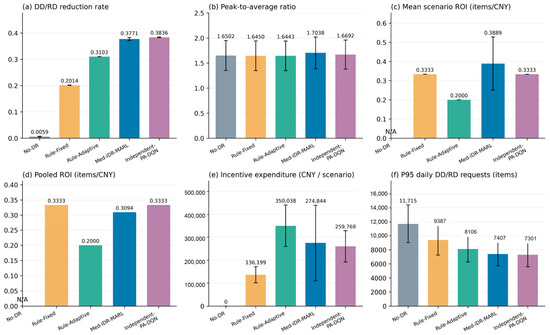
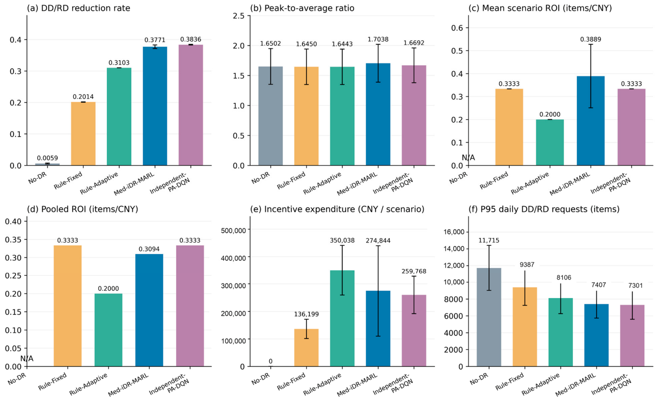
No-DR incurs zero incentive expenditure, so its ROI is undefined and is displayed as N/A. All incentive-paying methods have positive expenditure in every Table 3 scenario. Table 3 and Figure 2 are generated from the same 20-scenario result file.

Figure 2. Fixed-checkpoint baseline results, sharing the input of Table 3. Error bars are descriptive SDs across 20 scenarios; pooled ROI has no scenario SD. N/A indicates that ROI is undefined for the No-DR baseline because no incentive expenditure is incurred.

No-DR had a mean schedulable-demand reduction of 0.0059 and 14,365.38 over-quota requests per episode. Rule-Fixed and Rule-Adaptive eliminated over-quota requests, with reductions of 0.2014 and 0.3103, respectively. Med-iDR-MARL reduced demand by 0.3771 and spent CNY 274,844.23 per scenario on average, compared with CNY 350,038.43 for Rule-Adaptive.

Independent-PA-DQN achieved a slightly higher reduction (0.3836 vs. 0.3771) and lower mean expenditure (CNY 259,768.38 vs. CNY 274,844.23) than Med-iDR-MARL; both had zero over-quota requests. Mean scenario ROI favors Med-iDR-MARL (0.3889 vs. 0.3333 items/CNY), but pooled ROI favors Independent-PA-DQN (0.3094 vs. 0.3333). One plausible explanation is that its hospital agents were trained under a stable CNY 3 incentive, whereas the hierarchical model adds a changing regional signal and joint-learning non-stationarity; the extra flexibility did not improve this test comparison. This mechanism was not isolated experimentally, so the explanation remains a hypothesis. The apparent ROI ranking depends on aggregation, and the hierarchical method does not dominate this learning baseline on the combined outcomes. A diagnostic re-evaluation using the MARL-saved beta matrix as the common test matrix, with policy weights unchanged, did not reverse the ordering: Independent retained greater reduction (0.3823 vs. 0.3777), lower expenditure (CNY 258,901.92 vs. CNY 275,180.75), higher pooled ROI (0.3333 vs. 0.3093), and lower PAR (1.6708 vs. 1.7128). Because each common matrix matches only one policy’s saved coefficients, this diagnostic does not remove the unmatched-training limitation.

Med-iDR-MARL had the highest PAR (1.7038), exceeding No-DR (1.6502) and Independent-PA-DQN (1.6692). Compared with No-DR, however, its mean absolute daily peak fell from 12,047.39 to 7797.10 items, and its mean daily request fell from 7476.66 to 4685.04; mean P95 fell from 11,714.60 to 7406.74. A larger proportional decline in the mean than in the residual peak can increase PAR despite lower absolute demand. Incentive timing and DD state dynamics may concentrate residual requests, but their causal roles were not isolated here. Relative concentration remains a planning drawback for inventory and transport capacity; zero over-quota requests do not establish peak smoothing.

The re-evaluated mean DD counters are 0.7318 for MARL and 0.6128 for Independent, compared with 0.2238 and 0.1776 reported in the earlier baseline materials; reported maxima changed from 2 and 1 to 4. Meanwhile, normalized RD dissatisfaction is approximately 0.0009 and 0.0011. This comparison reveals a DD/RD service trade-off, not improvement in all service measures. Because historical code and trajectories are incomplete, the changes cannot be attributed solely to repair rather than to other evaluation differences. Counter value four is a modeled state and is not itself evidence of a violated clinical waiting-time limit.

Mean scenario ROI and pooled ROI answer different questions: the former weights each scenario equally, whereas the latter is weighted by expenditure. Their different rankings in Figure 2 preclude an unqualified claim of superior incentive efficiency.

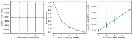
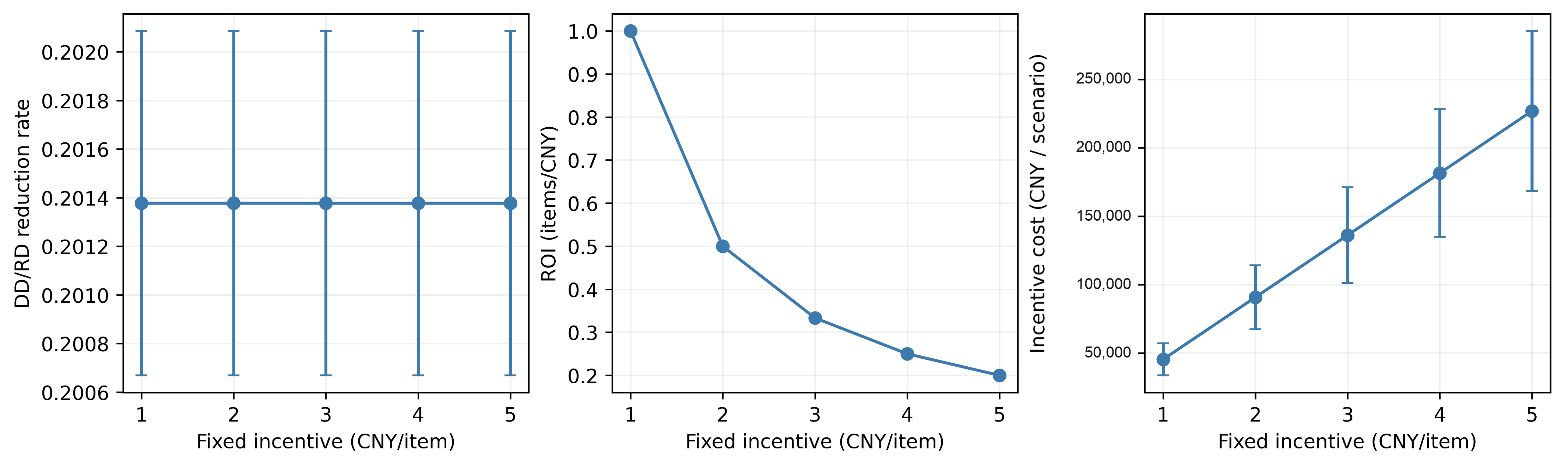
Figure 3 summarizes the historical Rule-Fixed incentive sweep across five positive incentive levels. The sweep is a diagnostic of the specified Rule-Fixed response, whose hospital request-rate rule remains unchanged across positive incentive levels. Thus, higher payments increase expenditure without changing reductions under this rule; the result is not evidence that actual hospitals are unresponsive to higher incentives. Its original environment seed and execution version were not archived, so this retained diagnostic is not treated as a replication of Table 3.

Figure 3. Historical Rule-Fixed incentive sweep: means ± descriptive SD across 20 scenarios per incentive. The programmed hospital response is unchanged for positive incentives.

5.3. Multi-Seed Training and Stochastic Stability

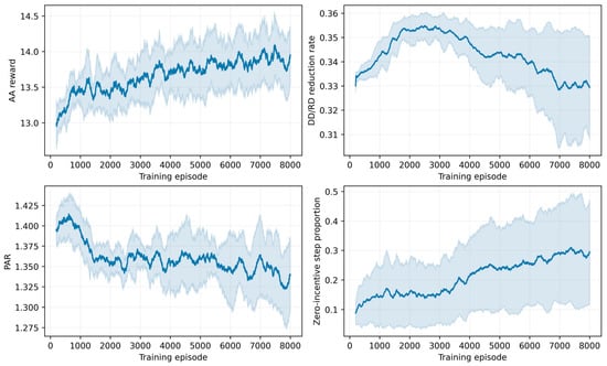
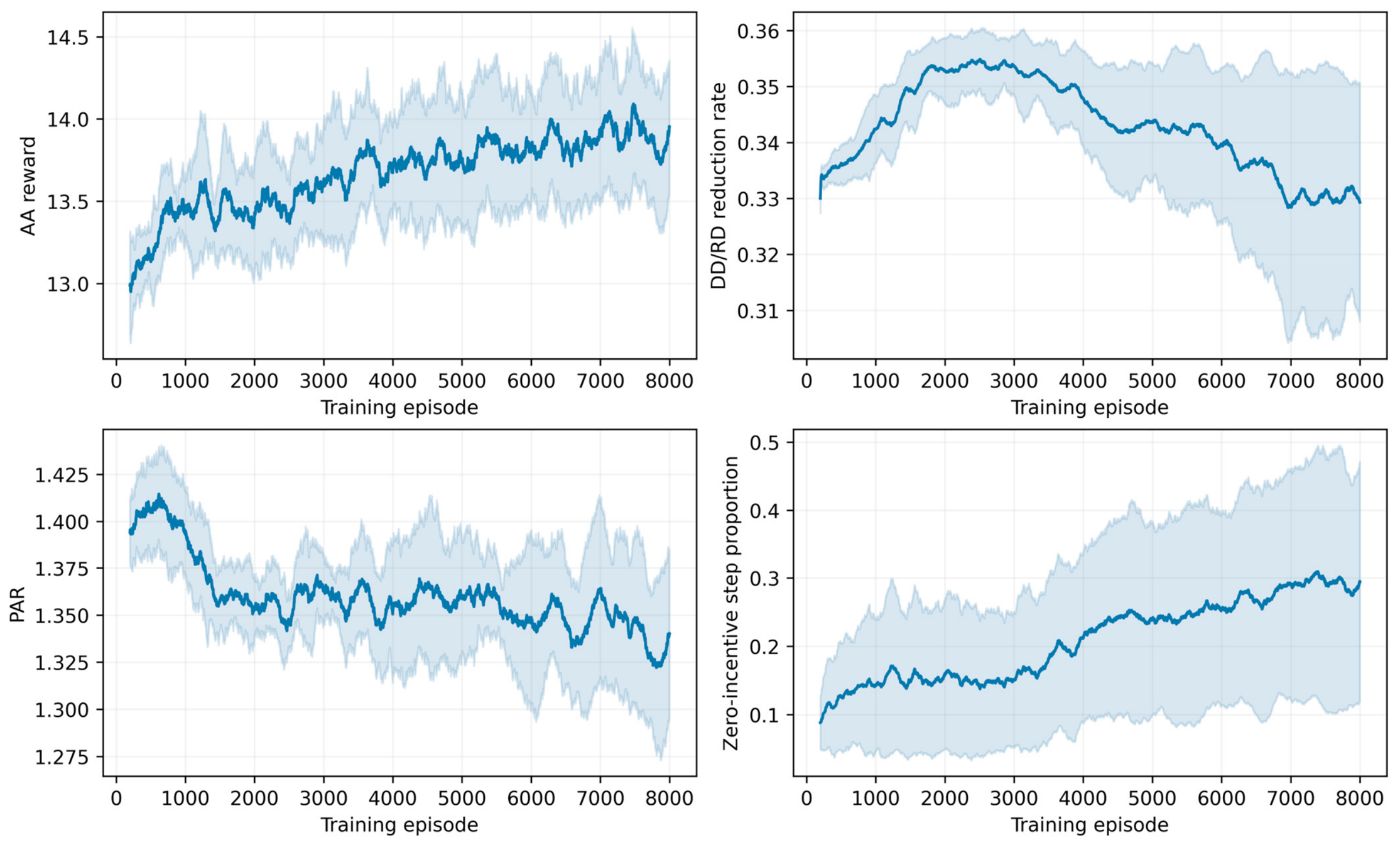
Table 4 and Figure 4 retain the earlier 10-seed training experiment. Each Table 4 observation is one seed’s mean over its final 1000 of 8000 episodes; these are training summaries, not held-out evaluations of the repaired policies. Figure 4 uses a 200-episode moving average for each seed and then plots the cross-seed mean and sample SD. This historical diagnostic should not be used as an additional replication of Table 3 or Table 6. The historical code and dependency versions cannot be authenticated from the retained traces; current code defaults are not used to fill that gap.

Figure 4. Earlier 10-seed training: 200-episode moving means with cross-seed sample SD shading.

Across the 10 seed-level late-training averages, reduction was 0.3303 ± 0.0217, ranging from 0.3049 to 0.3609. PAR was 1.3400 ± 0.0370. The SDs are recomputed consistently with the cross-seed convention used in the revised tables.

The historical traces describe variation in training reward, reduction, PAR, and zero-incentive use. They do not establish convergence, held-out generalization, or stability under the currently audited implementation.

5.4. Hospital Response Sensitivity and Coefficient Analysis

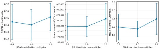
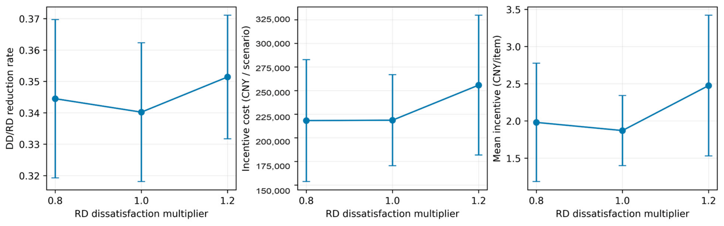
The earlier beta-sensitivity cohort varies the RD dissatisfaction coefficient by ±20% across 10 training seeds and evaluates each trained condition over 20 test windows. It is retained as a within-cohort exploratory analysis. Table 5 and Figure 5 report reduction, expenditure, and incentive rates. Scenario-level costs were not retained for auditing the zero-cost convention of the historical ROI summaries, so those ROI fields are not used for the revised economic comparison. The current script creates a fresh model for each condition and seed, but the retained historical output does not establish its exact training budget or scheduler version. Results were retained, not reproduced, under the present audit configuration.

Figure 5. Earlier 10-seed beta sensitivity: means with sample SD across seed-level scenario averages.

Reduction remained near 0.34–0.35 across the three conditions, while the mean incentive rate rose from 1.9807 at β × 0.8 to 2.4757 at β × 1.2. The middle condition was not monotonic (1.8708 at β × 1.0). These seed-level summaries support sensitivity to the assumed RD cost, not to an estimated hospital response curve or a statistically established causal effect.

5.5. Ablation Analysis

The ablation study was rerun for this revision. Full and six variants were each trained from initialization for 8000 episodes under seeds 0, 7, 21, 42, and 99, followed by 20 evaluation windows for each trained policy. The run logs and seed metadata support all 35 completed runs. The 35 seed summaries agree with the worker output files. However, executable model weights and hospital-day trajectories were not retained with this cohort, and metric files named checkpoint_*.json are not network checkpoints. Table 6 reports seed-level efficiency statistics and Table 7 reports the service metrics accumulated by the evaluator. Their aggregate consistency is verified, but the original stepwise outcomes cannot be independently replayed.

The current variant definitions are: without DCKP, use simple_schedule while retaining ND and the service floor; without risk, remove explicit risk observation and reward weighting while retaining risk-driven demand and quota; without heterogeneity, use tier-2 hospitals with scale 1 and α = 0.7 and a common hospital-level beta mean; without smoothing, remove the incentive-change limit; without soft-top3, disable that sampling option; without the service guard, set the scheduling floor to zero while retaining ND priority. Resource-level beta perturbations remain in the homogeneous condition. The last condition is evaluated against the original tier-specific floor. These changes apply to training and testing in the supplied training script, not only to test-time actions.

Within-seed pooled ROI divides total reduction by total expenditure across its 20 scenarios. We then summarize those five seed ratios. Logged means of scenario ROI are omitted because zero-cost scenarios were encoded as zero and the scenario records needed to revise that convention were not retained. All variants now report zero over-quota requests; without complete earlier trajectories, that change cannot be assigned to one implementation change.

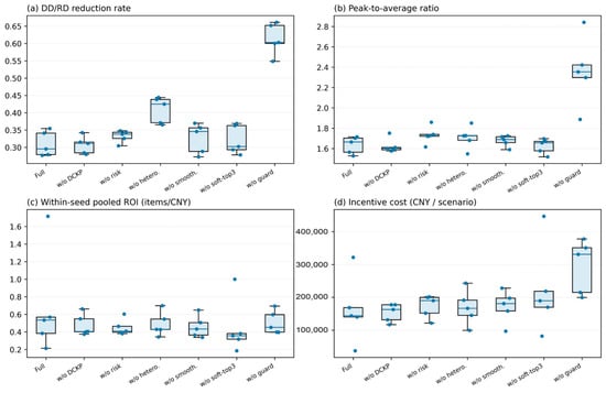
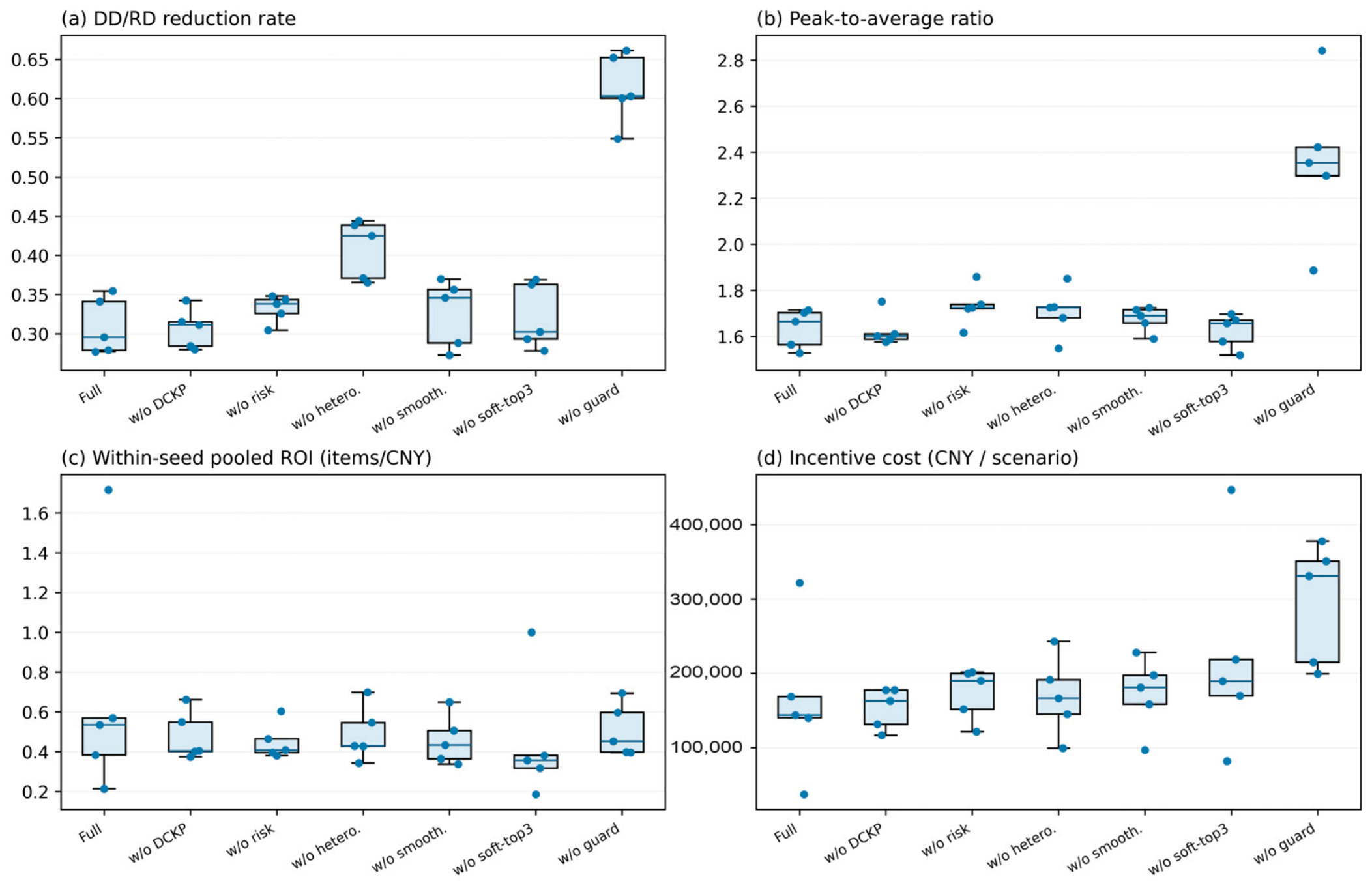
The full model achieved a reduction of 0.3093, a PAR of 1.6348, a within-seed pooled ROI of 0.6833, and zero over-quota requests (Table 6; Figure 6). Removing DCKP produced a similar reduction (0.3065) and PAR (1.6256), a lower pooled ROI (0.4781), and a greater normalized RD cost, but lower expenditure and a smaller mean DD counter. Thus, the scheduler did not improve every outcome. The full model’s pooled-ROI SD was 0.5942 across only five seeds, so these differences are descriptive. Some other removals increased reduction; service outcomes must be considered jointly.

Figure 6. Five-seed ablation.

Points show all seed summaries; boxes span the interquartile range (IQR) with a median line. Whiskers end at the most extreme observed values within 1.5 IQR; values outside of them remain visible as seed points. ROI is pooled within each seed.

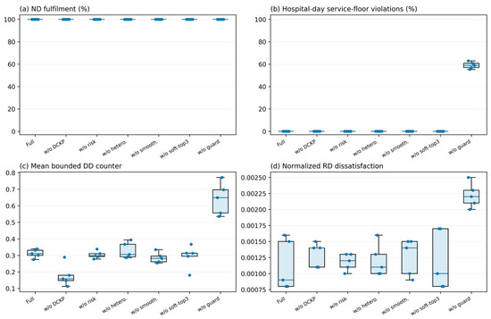
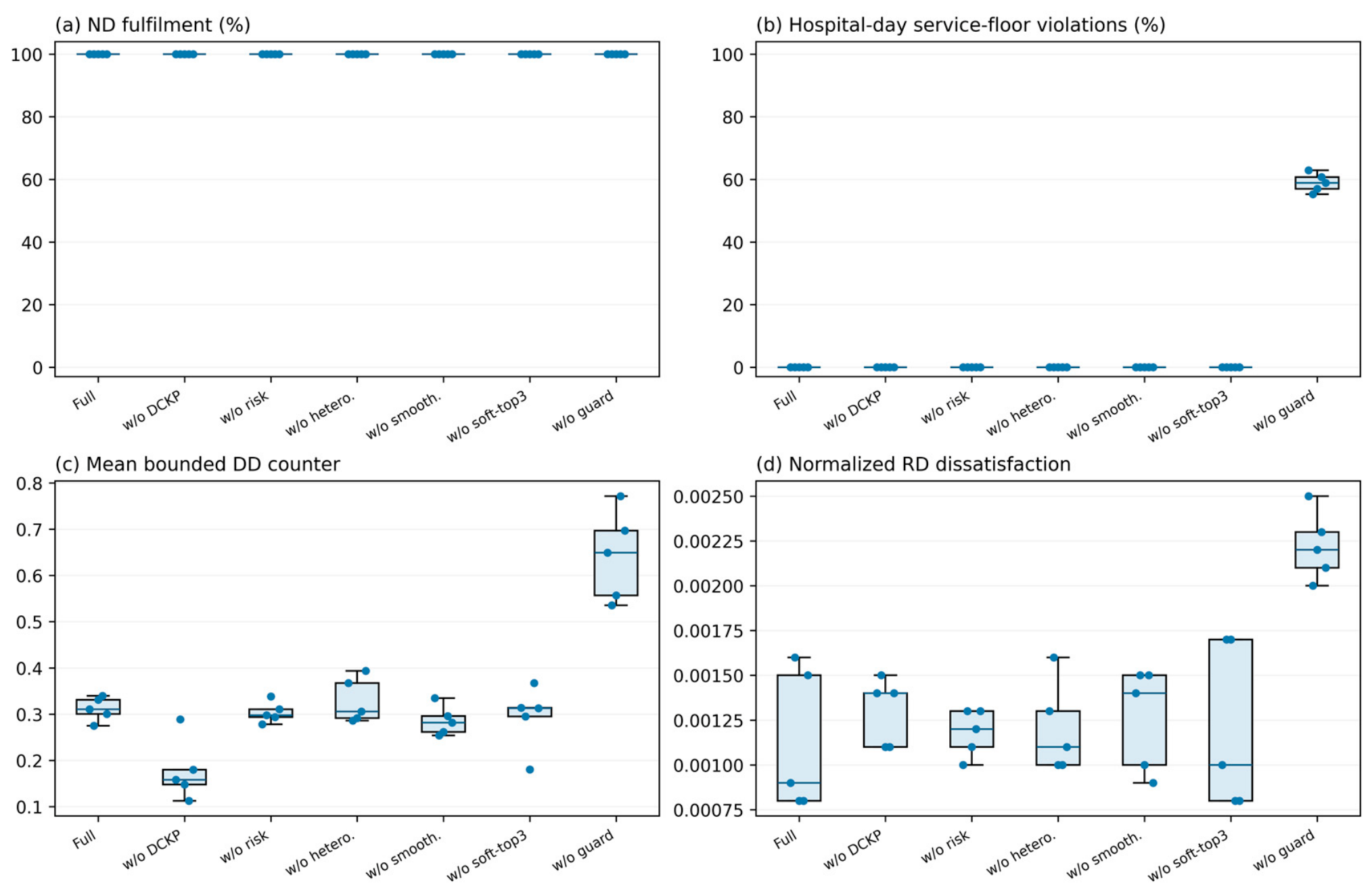
Removing the minimum-service guard increased reduction to 0.6130 and PAR to 2.3604, with a hospital-day violation rate of 58.95% versus zero for full (Figure 7). All variants retained ND by construction. This comparison describes the role of the explicit service floor, rather than a learned guarantee of clinical safety.

Figure 7. Five-seed service outcomes: ND retention, hospital-day service-floor violations, DD counter, and normalized RD cost. Points denote seeds; boxes and whiskers follow Figure 6.

5.6. Local Scheduler Diagnostics

Table 8 reports a new audit of 132,000 local states: 11 fixed request rates × 20 windows × 30 days × 20 hospitals, with NumPy seed 2026. Each rate follows its own repaired-DCKP trajectory, so its delay states can differ. At each recorded state, we compare the current implementation, the current greedy routine with only the interval-repair block removed, and exact enumeration of all 484 actions using identical inputs, constraints, and objectives. All states were retained. The controlled removal is not an authenticated reconstruction of the historical scheduler. Source inputs, actions, objectives, bounds, feasibility, and repair flags were saved.

Table 8. Local feasibility, repair activation, and objective gaps (12,000 states per rate).

Request Rate	Repair Triggered	No-Repair Feasible	Repaired Feasible	Mean Absolute Gap	Mean Gap/Bound 5
0.0	100%	0%	100%	0.0000	0.00%
0.1	100%	0%	100%	0.0000	0.00%
0.2	90%	10%	100%	0.0169	0.34%
0.3	90%	10%	100%	0.0416	0.83%
0.4	90%	10%	100%	0.0325	0.65%
0.5	90%	10%	100%	0.0236	0.47%
0.6	50%	50%	100%	0.3559	7.12%
0.7	0%	100%	100%	0.6663	13.33%
0.8	0%	100%	100%	0.5465	10.93%
0.9	0%	100%	100%	0.1741	3.48%
1.0	0%	100%	100%	0.0023	0.05%

Repaired DCKP and exact enumeration were feasible in all tested states; repair was triggered in 73,200 decisions (55.45%). The gap is J_DCKP − J_exact, normalized as 100 × gap/5. The bound 5 follows from two DD terms ≤1 and two RD terms, each bounded by 1.5, with conditions checked for this sample. The largest mean gap was 0.6663, or 13.33% of the bound, at rate 0.7. This is not a maximum individual error or a relative-to-optimum error: mean relative gaps at rates 0.7 and 0.8 were 1043.40% and 1366.27%. At rate 1.0, all exact costs were zero, so relative gaps were undefined; those states were retained and their mean absolute gap was 0.0023. The non-monotonic pattern reflects rate-dependent feasible sets, repair activation, and trajectory states. It does not imply monotonic approximation quality.

Runtime was measured separately on 1320 preselected states: all rates and windows, day offsets 0 and 15, and hospital indices 0, 10, and 18. After warm-up, each function was called nine times per state in rotating order; other audit experiment processes had completed. Table 9 summarizes the per-state median times. Candidate grids were precomputed for both repair and exact enumeration. Timing excludes network inference, input generation, and serialization, and compares these implementations only.

Table 9. Local scheduler runtime on 1320 states (microseconds).

Implementation	Mean	Median	P95
Current greedy, repair removed	42.60	37.30	81.71
Current repaired DCKP	70.91	55.80	158.74
Vectorized exact enumeration	67.19	56.25	129.20

Note: Statistics summarize each state’s median of nine calls. Windows 11, Python 3.12.4 and NumPy 2.3.4; Intel64 Family 6 Model 126 Stepping 5, 8 logical CPUs. Background operating-system load was uncontrolled. Exact CPU product identification was unavailable.

Repaired DCKP and exact enumeration had similar median times (55.80 and 56.25 μs), while repaired DCKP had a larger mean and P95. The routine without repair was faster but often infeasible (Table 8). These measurements do not support a consistent repaired-DCKP speed advantage. DCKP is retained in the reported framework because the trained policies interacted with this scheduler; replacing it would define a different evaluation environment. At this four-category scale, vectorized exact enumeration is a viable alternative, and larger multi-item scalability remains untested. No infeasible action grid arose in the sample; the fallback behavior described in Section 4.4 remains a limitation outside of it.

6. Discussion

6.1. Managerial Implications of Demand-Side Request Regulation

The simulation separates incentive-driven request responses from subsequent physical allocation. Results depend on the programmed rules, learned policies, and assumed constraints; they do not show that supply-side allocation alone is insufficient in actual hospitals.

Relative to Rule-Adaptive, Med-iDR-MARL increased the mean reduction rate from 0.3103 to 0.3771 (6.68 percentage points) and lowered mean scenario incentive expenditure from CNY 350,038.43 to CNY 274,844.23 (21.5%). Against Independent-PA-DQN, however, it achieved a slightly lower reduction and higher expenditure; its ROI advantage appears only when scenario ratios are averaged, not when reduction and cost are pooled. The evidence supports a conditional comparison rather than a claim of overall economic dominance.

The mechanism can be studied as an input to subsequent replenishment, allocation, and transport models. However, its higher PAR and omitted logistics constraints mean that reduced requests cannot be assumed to yield smoother operations, fewer physical shortages, or lower total supply-chain cost.

Medical supply request regulation should be assessed jointly in terms of reduction and service protection. In the full-model ablation cohort, ND fulfillment was 1.0000, the minimum-service violation rate was 0.0000, mean bounded DD counter was 0.3112, and normalized RD dissatisfaction was 0.0011. Removing the minimum-service guard increased raw reduction from 0.3093 to 0.6130, but increased mean bounded DD counter to 0.6422, normalized RD dissatisfaction to 0.0022, and the minimum-service shortfall to 67,534.3 items per scenario. The corresponding violation rates were 66.39%, 54.68%, and 38.78% for Tier 3, Tier 2, and Tier 1 hospitals. ND fulfillment remained complete because ND priority is implemented separately from the total minimum-service floor. These simulated constraints do not establish clinical safety in practice.

6.2. Hospital Heterogeneity, Response Sensitivity and Privacy-Aware Deployment

The homogeneous condition increased reduction from 0.3093 to 0.4087, increased PAR from 1.6348 to 1.7066, and reduced within-seed pooled ROI from 0.6833 to 0.4886. It simultaneously changes hospital tiers, scales, service floors, and beta sampling; these differences cannot be attributed to a single factor. Compliance with different tier thresholds also does not establish equitable costs, reduction burdens, or patient outcomes.

The earlier beta analysis illustrates dependence on assumed hospital response costs. It does not establish how actual hospitals should be compensated. The current model uses a single regional incentive; differentiated incentives, institutional acceptability, and equity across patient groups require separate evaluations.

Aggregate AA observations reduce the raw records needed by the regional learner but provide no formal privacy guarantee. Implementation would require hospital-system interfaces, access controls, clinical review of demand categories, incentive funding and payment governance, abnormal-request review, staff training, and an assessment of hospitals’ willingness to participate. The model includes simulated incentive transfers; it does not price these implementation requirements, measure acceptance, or evaluate data-governance compliance.

6.3. Limitations and Future Research

First, the environment is simulated. The Shanghai series supplies only a normalized risk trajectory; simulated demand, quotas, hospital tiers, and incentive responses are not actual Shanghai hospital data. The 20-hospital network, risk-driven demand multiplier, service floors, and dissatisfaction coefficients require calibration and external validation against multi-hospital request, consumption, inventory, and patient-acuity records.

Second, the model neither identifies strategic request inflation nor tests panic, political pressure, bureaucratic rules, collusion, or refusal to respond to incentives. Its request-rate action is at most one relative to the exogenous baseline. General rationing theory [13,14,15] motivates the research question but cannot validate the behavioral assumptions. Hospital interviews and linked request, procurement, and consumption histories are needed; non-response and strategic-reporting stress tests remain future work.

Third, the model ends at local request regulation and does not represent procurement lead times, replenishment, supplier capacity, transport, stock expiration, substitution beyond the RD abstraction or redistribution of surplus. Incentive expenditure and items-per-CNY ROI are not a full economic cost or welfare analysis. Integration with inventory and logistics models is required before evaluating system-wide cost, shortage, and resilience effects [10,12,23].

Fourth, local feasibility, local objective quality, and end-to-end policy performance are separate questions. Table 8 and Table 9 show feasibility in tested states, material local objective gaps, and no consistent runtime advantage over the vectorized exact comparator. The repair includes enumeration and can retain an infeasible schedule when no feasible candidate exists. Cross-hospital and multi-period optimization was not assessed. The DD counter also omits a conserved backlog and terminal settlement, limiting its service interpretation.

Fifth, continuous-policy PPO, DDPG, and alternative action granularities were not benchmarked. Cohorts differ in training and evidence provenance: the baseline is reproducible under a common test beta that differs from the MARL-saved coefficients, while the historical training and sensitivity cohorts lack authenticated execution versions; the new ablation rerun has completion logs and seed summaries but no saved network weights or hospital-day trajectories. Overlapping windows from a series also used in training limit inference about unseen conditions. These constraints preclude a claim that all historical experiments were independently reproduced.

Future work should calibrate response and service assumptions with hospitals and integrate request regulation with procurement, inventory, allocation, and transport. Institutional acceptability, equitable burdens, and patient outcomes require separate evaluation.

7. Conclusions

Med-iDR-MARL connects regional incentives, heterogeneous hospital responses, and local ND/DD/RD scheduling before formal allocation. The fixed-checkpoint comparison shows lower requests and expenditure than Rule-Adaptive, but Independent-PA-DQN achieves greater reductions, lower expenditure, higher pooled ROI, and lower PAR. The hierarchical model’s advantage in mean scenario ROI does not establish overall economic dominance.

The separate five-seed ablation links removal of the service floor to a 58.95% hospital-day violation rate and a mean shortfall of 67,534.3 items per scenario. Local diagnostics found feasible schedules in 132,000 tested states but also material optimality gaps and no consistent runtime advantage for repaired DCKP. These findings support a conditional simulation comparison; they do not establish clinical safety, external validity, or deployment readiness.

References

- World Health Organization. Rational Use of Personal Protective Equipment for Coronavirus Disease (COVID-19) and Considerations During Severe Shortages: Interim Guidance, 23 December 2020; WHO: Geneva, Switzerland, 2020; Available online: https://www.who.int/publications/i/item/rational-use-of-personal-protective-equipment-for-coronavirus-disease-%28covid-19%29-and-considerations-during-severe-shortages (accessed on 16 September 2026).
- GOV.UK. PPE Portal: How to Order COVID-19 Personal Protective Equipment (PPE). 2023. Available online: https://www.gov.uk/guidance/ppe-portal-how-to-order-covid-19-personal-protective-equipment (accessed on 16 September 2026).
- Centers for Disease Control and Prevention; National Institute for Occupational Safety and Health. Personal Protective Equipment Burn Rate Calculator. 2024. Available online: https://www.cdc.gov/niosh/healthcare/hcp/pandemic/PPE-Burn-rate-calculator.html (accessed on 16 September 2026).
- ASPR TRACIE. Medical Operations Coordination Centers (MOCCs): Patient Load Balancing Summary of Lessons Learned During COVID-19. Available online: https://asprtracie.hhs.gov/technical-resources/resource/13008/medical-operations-coordination-centers-mocc-patient-load-balancing-summary-of-lessons-learned-during-covid-19 (accessed on 16 September 2026).
- Govindan, K.; Mina, H.; Alavi, B. A decision support system for demand management in healthcare supply chains considering the epidemic outbreaks: A case study of coronavirus disease 2019 (COVID-19). Transp. Res. Part E Logist. Transp. Rev. 2020, 138, 101967. [Google Scholar] [CrossRef] [Scilit] [PubMed]
- Liu, J.; Bai, J.; Wu, D. Medical supplies scheduling in major public health emergencies. Transp. Res. Part E Logist. Transp. Rev. 2021, 154, 102464. [Google Scholar] [CrossRef] [Scilit] [PubMed]
- Fattahi, M.; Keyvanshokooh, E.; Kannan, D.; Govindan, K. Resource planning strategies for healthcare systems during a pandemic. Eur. J. Oper. Res. 2023, 304, 192–206. [Google Scholar] [CrossRef] [Scilit] [PubMed]
- Spieske, A.; Gebhardt, M.; Kopyto, M.; Birkel, H. Improving resilience of the healthcare supply chain in a pandemic: Evidence from Europe during the COVID-19 crisis. J. Purch. Supply Manag. 2022, 28, 100748. [Google Scholar] [CrossRef] [Scilit]
- Wang, Y.; Lyu, M.; Sun, B. Emergency resource allocation considering the heterogeneity of affected areas during the COVID-19 pandemic in China. Humanit. Soc. Sci. Commun. 2024, 11, 225. [Google Scholar] [CrossRef] [Scilit]
- Götz, P.; Auping, W.L.; Hinrichs-Krapels, S. Contributing to health system resilience during pandemics via purchasing and supply strategies: An exploratory system dynamics approach. BMC Health Serv. Res. 2024, 24, 130. [Google Scholar] [CrossRef] [Scilit] [PubMed]
- Saha, E.; Rathore, P. A smart inventory management system with medication demand dependencies in a hospital supply chain: A multi-agent reinforcement learning approach. Comput. Ind. Eng. 2024, 191, 110165. [Google Scholar] [CrossRef] [Scilit]
- Lucas, T.C.; Guimarães, R.D.; Vasconcellos, M.S.G.; Lins, I.D.; Moura, M.J.d.C.; de Siqueira, P.G.S.C. Resilience of critical supply chains in pandemics: A model proposal for health personal protective equipment socially optimal distribution. Oper. Res. Health Care 2024, 40, 100420. [Google Scholar] [CrossRef] [Scilit]
- Lee, H.L.; Padmanabhan, V.; Whang, S. Information distortion in a supply chain: The bullwhip effect. Manag. Sci. 1997, 43, 546–558. [Google Scholar] [CrossRef] [Scilit]
- Cachon, G.P.; Lariviere, M.A. Capacity choice and allocation: Strategic behavior and supply chain performance. Manag. Sci. 1999, 45, 1091–1108. [Google Scholar] [CrossRef] [Scilit]
- Bray, R.L.; Yao, Y.; Duan, Y.; Huo, J. Ration gaming and the bullwhip effect. Oper. Res. 2019, 67, 453–467. [Google Scholar] [CrossRef] [Scilit]
- Cheraghi, S.; Haeri, A.; Ghannadpour, S.F. A dynamic and intelligent decision-making framework for a platelet inventory-distribution network. Oper. Res. 2025, 25, 66. [Google Scholar] [CrossRef] [Scilit]
- Komorowski, M.; Celi, L.A.; Badawi, O.; Gordon, A.C.; Faisal, A.A. The artificial intelligence clinician learns optimal treatment strategies for sepsis in intensive care. Nat. Med. 2018, 24, 1716–1720. [Google Scholar] [CrossRef] [Scilit] [PubMed]
- Coronato, A.; Naeem, M.; De Pietro, G.; Paragliola, G. Reinforcement learning for intelligent healthcare applications: A survey. Artif. Intell. Med. 2020, 109, 101964. [Google Scholar] [CrossRef] [Scilit] [PubMed]
- Bednarski, B.P.; Singh, A.D.; Jones, W.M. On collaborative reinforcement learning to optimize the redistribution of critical medical supplies throughout the COVID-19 pandemic. J. Am. Med. Inform. Assoc. 2021, 28, 874–878. [Google Scholar] [CrossRef] [Scilit] [PubMed]
- Lazebnik, T. Data-driven hospitals staff and resources allocation using agent-based simulation and deep reinforcement learning. Eng. Appl. Artif. Intell. 2023, 126, 106783. [Google Scholar] [CrossRef] [Scilit]
- Hernandez-Leal, P.; Kartal, B.; Taylor, M.E. A survey and critique of multiagent deep reinforcement learning. Auton. Agents Multi-Agent Syst. 2019, 33, 750–797. [Google Scholar] [CrossRef] [Scilit]
- Oroojlooy, A.; Hajinezhad, D. A review of cooperative multi-agent deep reinforcement learning. Appl. Intell. 2023, 53, 13677–13722. [Google Scholar] [CrossRef] [Scilit]
- Valizadeh, S.; Abbasi, B.; Nguyen, S.; Hosseinifard, Z. Platelet inventory management in hospital networks: A reinforcement learning approach. Transp. Res. Part E Logist. Transp. Rev. 2026, 208, 104629. [Google Scholar] [CrossRef] [Scilit]
- Yuan, Y.; Du, L.; Luo, L.; Cui, L. Allocation strategy of medical supplies during a public health emergency: A tripartite evolutionary game perspective. Sci. Rep. 2023, 13, 9571. [Google Scholar] [CrossRef] [Scilit] [PubMed]
- Myerson, R.B. Optimal auction design. Math. Oper. Res. 1981, 6, 58–73. [Google Scholar] [CrossRef] [Scilit]
- Bai, L.; Zhang, J. An incentive-based method for hospital capacity management in a pandemic: The assignment approach. Int. J. Math. Oper. Res. 2014, 6, 452–473. [Google Scholar] [CrossRef] [Scilit]
- Brero, G.; Eden, A.; Chakrabarti, D.; Gerstgrasser, M.; Greenwald, A.; Li, V.; Parkes, D.C. Stackelberg POMDP: A reinforcement learning approach for economic design. arXiv 2022, arXiv:2210.03852. [Google Scholar] [CrossRef] [Scilit]
- Ning, Z.; Xie, L. A survey on multi-agent reinforcement learning and its application. J. Autom. Intell. 2024, 3, 73–91. [Google Scholar] [CrossRef] [Scilit]
- Albadi, M.H.; El-Saadany, E.F. A summary of demand response in electricity markets. Electr. Power Syst. Res. 2008, 78, 1989–1996. [Google Scholar] [CrossRef] [Scilit]
- Siano, P. Demand response and smart grids—A survey. Renew. Sustain. Energy Rev. 2014, 30, 461–478. [Google Scholar] [CrossRef] [Scilit]
- Vardakas, J.S.; Zorba, N.; Verikoukis, C.V. A survey on demand response programs in smart grids: Pricing methods and optimization algorithms. IEEE Commun. Surv. Tutor. 2015, 17, 152–178. [Google Scholar] [CrossRef] [Scilit]
- Lu, R.; Hong, S.H.; Yu, M. Demand response for home energy management using reinforcement learning and artificial neural network. IEEE Trans. Smart Grid 2019, 10, 6629–6639. [Google Scholar] [CrossRef] [Scilit]
- Yu, L.; Xie, W.; Xie, D.; Zou, Y.; Zhang, D.; Sun, Z.; Zhang, L.; Zhang, Y.; Jiang, T. Deep reinforcement learning for smart home energy management. IEEE Internet Things J. 2020, 7, 2751–2762. [Google Scholar] [CrossRef] [Scilit]
- van Tilburg, J.; Siebert, L.C.; Cremer, J.L. MARL-iDR: Multi-agent reinforcement learning for incentive-based residential demand response. arXiv 2023, arXiv:2304.04086. [Google Scholar] [CrossRef] [Scilit]
Disclaimer/Publisher’s Note: The statements, opinions and data contained in all publications are solely those of the individual author(s) and contributor(s) and not of MDPI and/or the editor(s). MDPI and/or the editor(s) disclaim responsibility for any injury to people or property resulting from any ideas, methods, instructions or products referred to in the content. |
© 2026 by the authors. Licensee MDPI, Basel, Switzerland. This article is an open access article distributed under the terms and conditions of the Creative Commons Attribution (CC BY) license.