


Abstract
Generalized aquifers are widely used in various fields, such as groundwater use, mine water prevention and control, and geothermal energy. This paper presents a transformer-model-based automatic aquifer generalization method using borehole logs in scenarios with scarce experimental parameters. Relying only on basic borehole data, the method used an agent-assisted approach to extract and clean key lithological and coordinate information, which was then fused using a dual embedding mechanism. The model leveraged multi-head self-attention to calculate attention weights between the target stratum and its adjacent strata, capturing the potential contextual correlations in aquifer potential across strata. The resulting deep feature vectors from the transformer’s encoder were fed into a classification head to predict aquifer potential labels. Evaluation results demonstrated a model accuracy of 0.86, significantly outperforming the random classification baseline in precision, recall, the F1-score, and the kappa coefficient.
1. Introduction
Generalized aquifers are widely used in various fields, such as groundwater use, mine water prevention and control, and geothermal energy [1,2]. Borehole logs, which act as high-resolution sampling windows into complex subsurface systems, provide accurate stratigraphic constraints for building and conditioning numerical models [3,4]. However, classifying hydrostratigraphy from drilling lithology alone has limitations, and typically, additional field tests and investigations are required to identify dominant regional attributes, conceptualize aquifers and aquitards, and establish defensible parameter zonations for simulation [5,6,7]. Aquifer generalization methods have advanced substantially over the past two decades, and the toolbox has continued to evolve [8]. At many mining sites, cost and terrain constraints prevent sufficient step-drawdown or multi-level pumping tests and other in situ measurements, and key parameters, such as hydraulic conductivity, are sparsely observed [9,10]. Under such data-scarce conditions, reliably determining hydrostratigraphic water-bearing properties and improving conceptual model credibility using only existing boreholes and legacy hydrogeological reports remain major practical challenges [11,12].
Existing aquifer generalization methods are categorized into traditional experience-based and modern algorithm-driven methods (Table 1). Traditional experience-based methods focus on manual stratification and empirical parameter assignment. The manual stratification (or artificial experience) method relies on the experience of hydrogeological professionals. The boundaries of aquifers, such as borehole core logging, are directly delineated using paper data. This method is applicable to situations in which geological conditions are simple and data are extremely scarce [1,13,14]; however, the results are prone to subjective perceptions, making it difficult to characterize complex geological bodies [5]. Empirical parameter assignment is based on the statistical correlation between lithology and parameters; although easy to operate, such assignment often ignores the permeability differences within the same lithology and connectivity structures and fails to effectively reflect heterogeneity [15,16]. In contrast, modern algorithm-driven methods are further subdivided into four categories: geostatistical, machine-learning-driven, multi-source data fusion, and dynamic process coupling methods. Geostatistical methods, which focus on transition probability and kriging, are used to construct hydrostratigraphic models by quantifying spatial correlation [17]. However, these methods are sensitive to borehole density and data quality, and their performance is limited in heterogeneous aquifers with low normal distribution patterns or high connectivity. Machine-learning-driven methods, such as support vector machines and convolutional neural networks used for lithology prediction, explore the nonlinear correlations of multi-source data and build surrogate models [18]. However, they are sensitive to the representativeness of the training data and noise characteristics, and their generalization ability is restricted by scarce data or distribution shifts [19]. Multi-source data fusion methods include the joint constraint of “borehole–geophysical exploration” under the Bayesian framework [7] and ensemble smoothing multiple data assimilation (ES-MDA) [20], which can improve generalization robustness. However, these methods are limited by prior uncertainty propagation and the matching of multi-scale observations. Dynamic process coupling methods perform temporal correction by coupling multiple fields combined with time-varying observations and are suitable for mining-affected areas or scenarios with intensive pumping and injection [21,22]. In recent years, the emerging InSAR-driven Bayesian pore elasticity inversion has made it possible to convert large-scale surface deformation information into time-varying aquifer parameter fields [23,24].
Table 1.
Comparison of advantages and disadvantages of existing aquifer generalization methods.
In the fields of hydrogeology and geological engineering, machine learning methods for non-sequential (static or quasi-static) spatial samples can be broadly categorized into three paradigms: grid-based Convolutional Neural Networks (CNN) [25,26], Graph Neural Networks (GNN) [27,28], and text-based classification networks. Grid-based CNN methods typically interpolate boreholes or geological attributes onto regular grids before applying 2D/3D convolutions to exploit locally translation-invariant spatial patterns. While effective in remote sensing or dense-grid scenarios, they suffer from interpolation-induced bias and information loss when applied to sparse, irregular borehole networks [29]. In contrast, common GNN methods treat sampling points as fundamental objects, performing message passing or relative-coordinate kernel learning on irregular topologies via adjacency or point cloud operators. This paradigm is naturally suited for irregular sampling. However, its core limitation lies in “compressing” continuous spatial field information into discrete node features or edge structures, which poses challenges when requiring the preservation of multi-resolution field-level information or the direct utilization of large-scale geological fields [30]. Furthermore, existing work has also integrated lithological descriptions with deep classification models for core image classification, but often follows a two-stage approach: first performing independent classification of text or images, followed by spatial interpolation into the model. Few studies directly treat coordinate values and text embeddings as parallel, native inputs, allowing the model to learn their coupled representation [31].
This paper proposed a transformer-model-based automatic method of aquifer generalization using borehole logs under data-scarce conditions. The method relied only on the most basic borehole log data obtained by in-depth extraction of the “contextual information” between different boreholes. First, we established a data structure for extracting sample information and completed the extraction and cleaning of key information from borehole logs using an agent-assisted approach. Next, we labeled the aquifer potential characteristics of each stratum and fused the coordinate and lithological semantic information using a dual embedding mechanism. Subsequently, leveraging the multi-head self-attention mechanism of the transformer model, we calculated the attention weights between the target stratum and its adjacent upper and lower strata in both semantic and spatial dimensions, capturing the potential contextual correlation patterns in aquifer potential across strata. Finally, we input the deep feature vectors output by the transformer model’s encoder into the classification head to complete the category prediction of stratum aquifer potential labels and evaluated the model’s accuracy using metrics such as the confusion matrix and F1-score.
Compared to the aforementioned paradigms, the dual embedding a spatial weighting approach proposed in this study demonstrates three substantial differences and methodological innovations:
First, Hierarchical Separation of Representation Objects. Unlike common practices that either interpolate borehole coordinates into a regular grid or compress spatial information into node attributes before unified modeling, this study constructs two complementary types of latent representations in parallel at the input layer. One is a point-level digitized positional encoding, where normalized continuous numerical information such as X, Y coordinates, and cumulative depth is explicitly introduced into the Transformer as a position-related numerical embedding component. The other is a lithological text semantic embedding generated by a pre-trained language model, capturing the implicit attribute information within geological descriptions. By retaining both numerical spatial information and textual semantic information in parallel within the same model, it can simultaneously perceive spatial proximity relationships between boreholes and semantic associations between geological attributes when learning discriminative features for formation water richness, without the need for regularizing the original spatial sampling structure.
Second, Conditional Spatial Weighting. Differing from the translation-invariant convolution kernels based on regular grids in CNNs or the static weights reliant on predefined adjacency in GNNs, this study introduces a conditional, learnable spatial weighting mechanism within the Transformer architecture. This mechanism takes point-level embeddings and their relative spatial positional information as inputs, dynamically adjusting the information contribution of different neighboring boreholes through attention weights. Consequently, spatial correlations are no longer determined solely by geometric distance or fixed neighborhood structures but can vary with the semantic features and spatial locations of the samples. From a modeling perspective, this design generalizes traditional “message passing” or “convolution operations” into a form of sample-conditional adaptive kernel function. It enables the model to capture complex geological features such as spatial heterogeneity, anisotropy, and asymmetric influences without requiring grid-based interpolation.
Third, Native Multimodal Fusion of Text and Numerical Features. Unlike two-stage methods that treat lithological text either as pre-processed labels or as auxiliary post hoc features, this study achieves native fusion of text semantic embeddings and coordinate positional encodings within the model itself. Both types of features are fed simultaneously into the Transformer’s attention layers, allowing the calculation of attention weights to be co-regulated by both semantic similarity and spatial relative relationships. This design enables the model to directly learn multimodal contextual associations at the level of raw observations—“borehole description text + spatial coordinates”—without requiring manually defined rules for fusing text and spatial features. This significantly enhances the model’s comprehensive ability to represent the spatial distribution patterns of formation water richness.
2. Training Sample Data and Model Training Method
This study proposed a method for self-classifying geological aquifers using transformer models under geological borehole data-scarce conditions. The algorithm’s workflow is shown in Figure 1. This approach predicts geological formations at target points through the standardized extraction of critical data from borehole column charts, expert classification, and transformer model training. Integrating OCR and agent-based self-extraction methods significantly reduces labor costs for data acquisition. Weighted positional encoding of coordinates and existing segmentation mechanisms enable the model to effectively capture potential aquifer-related correlations within contextual sequences.
Figure 1.
Algorithm flowchart.
2.1. Extraction and Structuring of Drilling Data
Borehole logs contain rich stratigraphic information but are often stored as images, which are not directly usable for machine learning. To create a structured dataset, we defined a universal textual format, which contains: borehole name, location coordinates (X, Y), collar elevation, and for each stratum: sequence number, cumulative depth, rock name, and lithological description. The water content property of each stratum, serving as the classification label, was initially estimated via keywords and subsequently validated and calibrated by hydrogeological experts.
Conventional Optical Character Recognition (OCR) applied to borehole images often performs poorly on geological terminology and irregular layouts. To address this, we employed a large language model (LLM) guided by targeted prompts to interpret OCR-extracted text, significantly improving the accuracy of parsing complex stratigraphic data as shown in Figure 2. This agent-assisted extraction was followed by human verification to correct residual errors and ensure formatting consistency. This hybrid approach reduced manual preprocessing time by approximately 70% compared to fully manual extraction. It is worth mentioning that once the Transformer model completes its training, the generation of water content labels will no longer rely on keyword matching. This workflow can then seamlessly integrate with the model, leading to a substantial improvement in the accuracy of aquifer productivity labels and a significant reduction in the manual labor required for generalization.
Figure 2.
A representative sample output showing the transition from a raw borehole log image to the final structured text data via the intermediate steps of the workflow.
And then, the extracted data were encapsulated into a nested list-dictionary structure (the specific structural example refer to Figure 3). Each borehole is represented by a dictionary containing its metadata (name, coordinates) and a list of stratum dictionaries. Each stratum dictionary contains its characteristic data (elevations, rock name, description) and the water content label. This structure preserves hierarchical relationships and enables efficient data handling.
Figure 3.
Example of the nested list-dictionary data structure used to encapsulate all extracted information for a single borehole and its multiple strata.
2.1.1. Extracted Content
The agent-assisted extraction was implemented via a specialized, modular workflow on ByteDance’s Coze platform. Figure 2 provides a schematic overview of this complete pipeline, illustrating the sequential integration of its seven core modules. By integrating OCR, large language models (LLMs), and procedural code, the workflow enables customizable prompts and targeted adjustments while visually tracing the transformation from raw borehole logs, through key intermediate steps, to the final structured textual output.
- Input: Accepts borehole log images.
- Borehole Header Extraction: An LLM, guided by prompts, extracts the borehole name, surface elevation, and X/Y coordinates from the OCR text of the header section.
- Stratigraphic Information Extraction: Performs layer-by-layer scanning to extract stratum sequence number, cumulative depth, rock name, and lithological description text.
- Geological Terminology Correction: An LLM acts as a “geological expert” to correct terms that contradict common geological sense (e.g., correcting “grandio” to “granodiorite”).
- Format Conversion: Converts the corrected text data into a preliminary JSON format.
- Unified Data Structure: A Python program processes the JSON data to: (i) calculate stratum top and bottom elevations using surface elevation and cumulative depth; (ii) perform a preliminary keyword-based assessment of stratum water content; and (iii) encapsulate all data into a standardized nested structure. The design of this final data structure is illustrated in Figure 3.
- Output: Exports a structured text file for each borehole log.
2.1.2. Typical Errors and Impact on Model Performance
This extraction workflow offers distinct advantages but is also subject to several characteristic error modes that may influence downstream model performance. Its primary strengths include a significant reduction in manual extraction time and the ability of the LLM to contextually correct certain OCR errors—for instance, rectifying a misread ‘S’ back to the numeral ‘5’. Furthermore, the final processing and formatting are governed by deterministic Python code, which ensures output consistency and eliminates the randomness often associated with pure LLM generation, thereby guaranteeing structural reliability.
However, the workflow’s limitations arise mainly from image quality and OCR failures, introducing specific noise into the dataset. First, if the source image contains overlapping text lines due to drafting errors, the OCR output may become garbled, producing long, nonsensical character strings. Without manual intervention, these segments inject meaningless noise into the lithological descriptions, potentially distorting the model’s learning of semantic features. Second, critical errors occur when OCR incorrectly segments table cells, such as concatenating the values of cumulative depth and thickness into a single, erroneous number. This can lead to severe inaccuracies—even orders-of-magnitude errors—in calculated elevations, generating spatial outliers that corrupt the learning of geographical correlations. Third, the overlap of grid lines with text can cause further OCR corruption. Similar to the first case, this results in feature noise within the lithological descriptions. Collectively, these errors manifest as both label inaccuracies (in coordinates and derived elevations) and feature noise (in rock names and descriptions), which can degrade the model’s ability to learn the true relationships between lithology, spatial context, and aquifer productivity.
2.2. Post-Processing of Extracted Formats
The specificity of certain borehole columnar diagram contents may still result in minor errors in the extracted raw data. Therefore, manual secondary processing is required to avoid affecting the model input. However, experts must also verify the accuracy of the rock layer water content labels.
2.2.1. Data Format Content Cleaning
Data cleaning eliminates outliers and errors in raw data and ensures data quality. Three main issues should be addressed:
- Structural validation: modifying or deleting records with missing fields or format errors, such as those with empty coordinate values or missing water content labels. Corresponding supplements should be prepared based on the actual situation.
- Spatial logic validation: ensuring elevation values satisfy the principle that the roof is higher than the floor and correcting anomalous records that violate geological principles.
- Text standardization: unifying semantic description formats, removing irrelevant symbols, and correcting recognition errors.
2.2.2. Basis and Evaluation Criteria for Formation Water Content Correction
In this study, stratigraphic water content served as a key hydrological parameter derived through expert synthesis based on comprehensive regional hydrogeological reports, borehole logs, and structural cross sections. The determination process functioned as the target label for model training, closely aligning with the coal mine safety requirements and geological characteristics of the North China Plain. This section outlines the key reference factors for the assessment.
(1) Reference Data from Borehole Logs
- Lithological and thickness information: Descriptions of rock types, grain sizes, and structural features are closely related to the stratigraphic water content. Based on the thickness and lithological relationships of the adjacent upper and lower strata, multiple strata can be grouped into unified aquifer/aquitard sets. Thicker aquifers are more likely to form stable water flow pathways.
- Drilling fluid consumption: During drilling operations, the rate of fluid consumption serves as a direct indicator of the formation permeability. A sudden, significant increase in fluid consumption or fluid loss in a particular stratum indicates the presence of conduits, such as fractures or karst cavities, within that stratum. These features confer high permeability to the formation, making it highly likely to be an aquifer. Conversely, strata showing minimal or negligible consumption typically belong to impermeable layers or weakly permeable formations.
- Logging curves: Resistivity and natural gamma curves reflect the material composition and structural characteristics of formations. In the North China Plain, the Oligocene Gray Aquifer is rich in electrolytes and typically exhibits low resistivity, whereas impermeable layers, such as mudstone and shale, show higher resistivity. Natural gamma curves can be used to identify the clay content in formations. Formations with a high clay content show poor permeability and often serve as supplementary evidence for identifying impermeable or weakly permeable layers.
- Water level data: These data, presented as continuous broken lines in borehole logs, are key dynamic indicators of formation aquifer characteristics. Their trends, fluctuation ranges, and stability directly reflect the hydrogeological properties of formations at different depths. A rapid upward trend in a segment of the water level curve, followed by stabilization, typically indicates severe water storage and high transport capacity in that formation. Such formations may contain carbonate rocks with interconnected fractures, allowing the groundwater to rapidly recharge the borehole under hydrostatic pressure and swiftly raise the water level so that it is in equilibrium with the formation water table. This area can be preliminarily identified as an aquifer. Conversely, a consistently low water level curve with minimal fluctuations or a slight rise followed by long-term stability indicates significant groundwater isolation by the formation.
For example, dense mudstone formations with extremely low porosity and undeveloped fractures impede groundwater infiltration into boreholes, preventing an effective water level rise. These formations are typical aquitards. When the water level curve exhibits irregular fluctuations or a gradual decline, comprehensive evaluation with other indicators is required. Irregular fluctuations accompanied by brief local water level rises may indicate the existence of isolated minor fractures or dissolution cavities within the formation, capable of storing only minimal groundwater, indicating that the formation is a weakly permeable zone. If the water level continues to slowly decline, it likely indicates extremely poor permeability in the formation traversed by the borehole, coupled with no sustained groundwater recharge, further confirming the formation’s impermeable nature.
Furthermore, comparing the rate of change and stabilization duration of water level curves at different depths can help in delineating the boundaries between aquifer and impermeable layer groups. The water level curve abruptly shifting from gradual change to rapid ascent, followed by swift stabilization, typically corresponds to the transition interface from an impermeable or weakly permeable zone to an aquifer. Conversely, sudden transition of the water level curve from a stable state to a gradual decline or prolonged stagnation may indicate entry into an underlying impermeable zone. This entire analysis is based on the dynamic characteristics of continuous water level curves and, when corroborated with indicators, such as lithological thickness, flushing fluid consumption, and logging curves, significantly enhances the accuracy and reliability of assessing the hydrogeological conditions of exposed formations in boreholes.
(2) Structural Profile Reference Data
- Fault information: This information helps distinguish between extensional aquifer faults and compressional or filled impermeable faults, which serve as critical hydraulic conduits. The risk of faults connected to the Ordovician–Silurian aquifer becoming sources of bottomhole water ingress should be assessed.
- Fold structures: Synclinal structures often act as groundwater convergence zones. If these structures contain permeable strata, they readily form water-rich areas. Anticlines may cause groundwater to diverge toward the wings, reducing the local stratum water content. The scale, morphology, and stratigraphic combinations of the core and wings influence groundwater storage and migration.
- Stratigraphic contact relationships: Weathering fracture zones near unconformities often exist and may serve as groundwater migration pathways, warranting close attention.
(3) Reference Data for Hydrogeological Reports
- Characteristics of aquifers and aquitards: Defining the types, burial depths, thicknesses, and distributions of primary aquifers and aquitards aids in macroscopically characterizing groundwater systems and clarifying hydraulic connections.
- Pumping tests and hydrological parameters: Various parameters, such as mine water inflow, obtained from pumping tests directly quantify aquifer types and serve as the most intuitive indicators of the stratigraphic water-bearing capacity. Mine water inflow can also be estimated using the double-sided water collection corridor method calculation for a complete well with pressure conversion to no pressure, as shown in Equation (1). This calculation helps determine the water richness of the aquifer and the potential impact level of water hazards, in accordance with the classification standards for hydrogeological types of coal mines specified in the 2018 edition of the Detailed Rules for Coal Mine Water Control.
- Groundwater dynamics: The groundwater quality, water level, and recharge/discharge conditions should be analyzed to clarify groundwater flow systems and hydrochemical field distribution characteristics in order to determine the hydraulic connections and boundary conditions between aquifers.
- Textual description of structural information: This serves as supplementary diagnostic features for structural cross sections, including descriptions of fault characteristics and weathering fracture zones.
- Survey findings and recommendations: These are systematic conclusions regarding geological and hydrogeological conditions, groundwater dynamics, etc., aligned with coal mine water control requirements and regulations to clarify the logical correspondence between recommendations and findings, along with technical quantification bases.
2.3. Model Training
The classification of water content in borehole strata is a fundamental task in categorizing geological data features. The core challenge is in effectively integrating lithological semantic information with a spatial coordinate context to achieve precise generalization of geological structures. Traditional machine learning methods have limitations when handling high-dimensional semantic features and complex spatial correlations. In contrast, the transformer architecture within deep learning models leverages its powerful attention mechanism to simultaneously capture both global and local detailed features within data. Therefore, this study adopted a transformer as the foundational model. Through a modular design, we integrated multisource geological data and used an encoder-only structure to construct a classification model for automated aquifer delineation. The transformer model transforms textual semantic and spatial contextual features into unified vector representations and ultimately outputs the classification results by leveraging its self-attention mechanism to uncover the intrinsic relationships among features.
2.3.1. Transformer-Based Encoder-Only Architecture
As shown in Figure 4, our model adopted a transformer’s encoder-only architecture. This choice stemmed from the fact that aquifer classification fundamentally involves “semantic understanding + feature classification” rather than sequence generation. A complete transformer comprises an encoder and a decoder. The encoder focuses on the deep encoding of input features through bidirectional self-attention mechanisms, whereas the decoder performs conditional generation on input sequences via encoder–decoder attention.
Figure 4.
Transformer encoder structure [32].
We did not need to generate new sequences for aquifer classification. Instead, we encoded the input textual semantic features and spatial features into fixed-dimensional vectors and then output category labels via a classification head. Therefore, the encoder component only comprises a multi-head self-attention sublayer and a feed-forward neural network sublayer. Each layer incorporates residual connections and layer normalization, which enables progressive extraction of high-order features, culminating in a comprehensive representation of the sample through global pooling of the encoded results. This design simplifies the model structure and reduces computational costs. Simultaneously, bidirectional attention fully exploits the reciprocal dependencies among “textual descriptions, spatial locations, and stratigraphic attributes” within geological data, providing comprehensive feature support for classification tasks.
Regarding model interpretability, the model’s predictions for the water content of rock strata were entirely based on the token sequence composed of borehole sample parameters (Figure 5). This sequence encompasses two core types of influencing factors: text-based factors (e.g., rock names, lithological descriptions) and numerical factors (e.g., X- and Y-coordinates, absolute depth, formation thickness).
Figure 5.
Example of a context sequence used to determine the water-bearing characteristics of the target stratum. The sequence integrates the lithological and spatial features of the target stratum and its neighboring strata in the training borehole, as well as those of the nearest borehole, the second-nearest borehole, and farther boreholes.
Text-based factors serve as the direct basis for water-bearing predictions. The eight common lithologies (rock types) in the North China coal-bearing strata (Figure 6) show significant differences in water abundance. In addition, the detailed information included in lithological descriptions (e.g., “well-developed fractures” and “high porosity”) serves as a direct indicator of high water richness.
Figure 6.
Diagram illustrating the water richness characteristics of eight common lithologies in the North China coal-bearing strata, arranged in ascending order of water richness (from bottom to top) under normal conditions. Among them, “mudstone” can be considered the relatively impermeable layer with the lowest water richness (as, in reality, no rock is absolutely impermeable), while “conglomerate” represents the aquifer with the highest water richness.
Numerical factors capture the influence of the waterlogging of adjacent strata on the target stratum through the context self-attention mechanism of the transformer model. In geological engineering, water-bearing rock groups typically comprise multiple strata. The key to their classification lies in the hydraulic connectivity and hydrochemical characteristics between strata, which are not constrained by geological age but are determined by features such as water quality, temperature, and abundance. Therefore, capturing the hydraulic correlation between strata is essential for accurately classifying water-bearing rock groups. For example, within the same borehole (sharing identical horizontal and vertical coordinates), if the target stratum is a relatively thin aquifer and the adjacent strata above and below are relatively thick aquifers, all these strata are often grouped into the same water-bearing rock group. This principle also applies to adjacent strata on the same horizontal plane. The spatial adjacency of strata coordinates shown in Figure 7 directly corresponds to the weighted influence of such relationships on the water richness of the target stratum.
Figure 7.
Diagram illustrating the influence of adjacent strata on the water richness of the target stratum based on coordinate distance. The figure shows the level of attention by the model to each adjacent layer when the number of adjacent boreholes, K, is set to 3. The model incorporates information (e.g., coordinates) as input, then processes it through its self-attention mechanism for encoding and computation, and, finally, dynamically simulates and optimizes a weight distribution akin to inverse distance weighting, enhancing the estimation of the target stratum’s water richness. Adjacent strata with the closest planar and vertical distances receive greater attention, while those farther away receive less attention (attention levels from highest to lowest: red, orange, green, gray).
The design of the borehole context sequence in Figure 5 encapsulates these textual and numerical factors as input tokens for the transformer model. This ensures that the model’s learning targets fully align with the core elements of the task, laying the groundwork for interpretability analysis.
Regarding principles, the transformer model’s self-attention mechanism is central to achieving interpretability. The attention weights computed between different tokens quantitatively reflect the hierarchical association strengths illustrated in Figure 7. For strata within the same borehole, self-attention assigns higher weights to tokens representing adjacent strata. This corresponds to the model’s ability to capture correlations between lithological sequences and permeability characteristics, as shown in Figure 6, explaining how the lithological combinations of adjacent strata influence water content determination. For strata across different boreholes, self-attention assigns higher weights to tokens representing strata of the same lithology in spatially adjacent boreholes. This reflects the model’s use of cross-validation based on stratum features from multiple boreholes, clarifying the internal logic by which identical lithologies in neighboring boreholes enhance classification reliability.
Overall, the transformer model is not a “black-box” model in this task. The explicit linkage between its input sequence and task elements, coupled with the quantitative representation of core correlations through self-attention weights, allows every water-bearing classification result to be traced back to key task logics, such as lithological characteristics, stratigraphic sequences, and spatial correlations across multiple boreholes. This approach fully aligns with the actual principles governing water-bearing rock group classification in geological engineering.
2.3.2. Encoding Differences Between Coordinates and Elevation
At the context modeling level, the transformer model incorporates positional information into feature representations through positional encoding, which addresses the issue of the insensitivity of self-attention mechanisms to the input order. For geological data, borehole coordinates and stratigraphic elevations not only reflect spatial locations but also imply lateral continuity (between boreholes) and vertical correlations (within boreholes across strata). Transformer position encoding typically incorporates sine and cosine functions, as shown in Equation (2).
Here, represents the sequence position, denotes the dimension of position encoding, indicates even dimensions, and indicates odd dimensions. By mapping spatial coordinates into a similar encoding format, the transformer model effectively captures geological patterns, such as “similar lithology in adjacent boreholes” and “gradual lithological transition from top to bottom within the same borehole,” providing spatial constraints for aquifer delineation.
However, because of the fundamental differences in geological significance between the horizontal and vertical coordinates and the top and bottom elevations, differentiated encoding schemes are required to accurately capture the constraint information that they contain.
Weighted Encoding of Coordinates
The core function of borehole coordinates is to characterize the lateral continuity of strata. In the absence of significant tectonic disturbances, the lithological and aquifer properties of adjacent boreholes typically show high correlation, resembling the uniform lateral distribution of strata controlled by a single sedimentary facies. Therefore, the encoding of horizontal and vertical coordinates must emphasize “spatial neighborhood dependence,” as described next.
(1) Coordinate normalization: The horizontal and vertical coordinates of boreholes are large numerical values, whose absolute magnitudes significantly impact spatial position continuity. Therefore, we used linear normalization to preserve relative distance characteristics, calculated using Equation (3):
Here, and are normalized values; and are original values; and and represent the maximum and minimum coordinate values, respectively.
(2) Neighborhood weighted encoding: To determine the influence of distance on relevance, we first retrieved the nearest-neighbor boreholes for each borehole based on a KD-Tree. Next, we calculated the neighborhood distance between boreholes and assigned weights using a Gaussian decay function.
The steps in constructing a KD-Tree are as follows: First, determine the partitioning dimension by comparing the variance of the horizontal coordinate with that of the vertical coordinate across the entire dataset; the division calculation is shown in Equation (4):
where represents the coordinates of borehole within the current node; and denote the respective mean coordinates; indicates the number of boreholes in the node; and determines the optimal dimension for spatial partitioning at the current level by comparing the variance of all coordinates, , against the variance of coordinates, .
This method ensures each split maximizes data point dispersion, preventing tree structure degradation.
Second, divide the space into left and right subsets based on the median of the determined dimension. Merge the points below this value into the left subtree set and those above this value into the right subtree set, as shown in Equation (5):
Here, denotes the total number of observations in the dataset of coordinate values arranged in ascending order; the parity (odd or even) of determines the calculation method for the median, as specified in the piecewise formula; denotes the median value in the current dimension; represents the left subtree containing elements below the median, ; and represents the right subtree containing elements above the median.
Third, construct a KD tree recursively. At each recursive step, the algorithm iterates through aforementioned equations until a node contains only a single coordinate pair or becomes an empty set, terminating the recursion and forming a leaf node. This strategy ensures the structure adapts to the spatial distribution characteristics of the data, guaranteeing balanced and efficient partitioning [33].
Finally, calculate the distance weight, , using a Gaussian decay function, as defined by Equation (6):
Here, represents the total number of boreholes, represents the distance between neighboring boreholes i and j, and represents the standard deviation of the Gaussian decay function.
(3) Horizontal position encoding: Normalized coordinates with neighborhood weights were fused into a high-dimensional vector, using an improved position encoding function:
where denotes the planar dimension parameter of the positional encoding vector. The first two components reflect continuity through neighborhood weighting, while the latter two preserve absolute positional information, effectively capturing geological logic, such as the water content of the target formation relative to surrounding formations.
Weighted Encoding of Elevation
Elevation coordinates differ slightly from planar coordinates, describing three core aspects: vertical stratigraphic relationships (e.g., the upper and lower continuity of “aquifer groups”), stratigraphic thickness characteristics (where bed thickness is determined by the elevation of its top and bottom surfaces), and sedimentological patterns (e.g., the depth dependence of limestone aquifers). Compared with planar coordinates, elevation coordinates maintain a tighter connection with depth and adjacent stratum information. Stratigraphic layers are typically few in number and minimally influenced by tectonics, eliminating the need to constrain the transformer model with a fixed k value for neighboring layers. We achieved optimal classification weight allocation through full stratigraphic positioning combined with the transformer model’s self-attention mechanism. Therefore, the elevation-encoding design process was as follows:
(1) Thickness calculation and normalization: The key indicator of formation thickness was directly quantified using Equation (8) and normalized to the range :
Here, represents the top elevation of layer (, where k is the total number of strata in this borehole) , denotes the bottom elevation of layer . represents the thickness of layer . are normalized values and and represent the maximum and minimum thickness of the borehole layer, respectively.
(2) Depth factor encoding: The depth exponential function, Equation (9), was introduced to capture sedimentological laws, using the top elevation, , as the variable:
Here, denotes the rate parameter. Smaller values (greater depth) yielded larger values, amplifying the weighting of specific lithologies at depth.
(3) Longitudinal position encoding: We integrated the thickness, roof/floor elevation, and depth factors to construct the encoding vector, as shown in Equation (10):
Here, denotes the vertical dimension parameter of the positional encoding vector. The first two components preserve the absolute stratigraphic information of the cap and base, while the latter two components, through interaction between depth factor and thickness, enhance the distinguishing features of “deep thick layers” and “shallow thick layers.” For example, when the target stratum is flanked by thick aquifer layers, even if its lithology resembles a water-stop layer, its encoding vector still exhibits high similarity with the overlying and underlying strata, supporting the joint delineation of “aquifer groups.”
Due to the complex tectonic and sedimentary phase transitions, directly determining the lateral-to-vertical weight ratios is challenging. Therefore, we added a single-head attention module after the spatial encoding layer. This module treats and as two “feature sources and calculates the attention weights for each source’s contribution to the current sample classification task. We set the query vector of this attention module to (where denotes vector concatenation and represents a linear transformation layer), and the key vector and value vector were both constructed directly from the positional encodings of the two feature sources (i.e., , ). Based on these definitions, attention weights corresponding to the current sample classification task were (where and are the weights for and , respectively). Their calculation process is shown in Equation (11):
Here, represents the key vector dimension () used to scale attention scores to prevent gradient vanishing. The final fused spatial encoding interval formula is given by Equation (12):
2.3.3. Text Semantic Word Embedding
At the semantic understanding level, the core challenge in rock naming and lithological description is transforming unstructured text into quantifiable semantic vectors. This paper used a pre-trained tokenizer—BERT’s Tokenizer—to standardize text processing. First, the original text was segmented into tokens (e.g., splitting “white medium-grained sandstone” into “grayish-white,” “medium-grained,” and “sandstone”). Each token was then mapped to a unique index value via vocabulary mapping. Finally, an embedding layer generated a word vector matrix (where represents the number of tokens and denotes the embedding dimension).
Subsequently, the corresponding word vector matrix and spatial position encoding were entered into the encoder-only model. The fused input features underwent linear transformation to generate the query matrix , the key matrix , and the value matrix .
2.3.4. Core Network Module of the Transformer Model
The transformer model captured the correlations across these three matrices via its multi-head self-attention mechanism. Equation (13) mathematically expresses the self-attention mechanism.
The multi-head attention mechanism enabled the model to focus on different subspaces through self-attention. While maintaining the overall number of parameters, multi-head attention divided the three parameters , , and into multiple groups. Each group was mapped to distinct subspaces within the high-dimensional space to compute the self-attention weights, allowing the model to simultaneously attend to different parts of the input. After multiple parallel computations, outputs from multiple heads were concatenated via linear transformations to form the complete multi-head attention result, restoring the original feature dimension. Because self-attention distributions vary across subspaces, multi-head attention identified correlations from different perspectives within the input data, capturing richer feature information, such as recognizing water content correlations between adjacent strata. The multi-head attention mechanism is expressed in Equation (14):
Subsequent residual connections prevented gradient vanishing, ensuring that the sample lithological features propagated to the final layer. Layer normalization standardized features stabilized the input distribution for subsequent network layers, and accelerated model convergence. Normalized features entered the forward propagation network and underwent two layers of linear transformations and nonlinear activations. This process first expanded the feature dimension before restoring it, capturing complex correlations and supplementing additional relevant details. Subsequently, this process was repeated multiple times (the value of Num Layers) to progressively refine lithological semantic correlations, stratigraphic vertical continuity features, and even global associations between spatial and semantic domains. After six layers of encoding, the model extracted the global features of the token at the beginning of the input sequence. These were fed into the classification head to obtain the probability distributions for each category. Finally, through cross-entropy loss calculation and back-propagation of the parameters using the Adam optimizer, the model was iteratively updated over several training epochs to converge to a stable classification performance.
2.3.5. Hyperparameters and Performance Evaluation Metrics
Model hyperparameters, such as the number of multi-head attention heads, the embedding dimension, stacking layers, and the learning rate, were tuned through a random search combined with validation set performance evaluation. During training, we computed metrics such as accuracy and loss on an independent validation set to select the hyperparameter combination that yielded the optimal validation performance.
Upon training completion, common classification evaluation metrics, such as confusion matrices, receiver operating characteristic (ROC) curves, accuracy, recall, the F1-score, and the kappa coefficient, were applied to assess model performance on the test set.
Here, TP (true positive) represents the number of samples correctly predicted as positive by the model, TN (true negative) represents the number of samples correctly predicted as negative, FP (false positive) represents the number of negative samples incorrectly predicted as positive, and FN (false negative) indicates the number of positive samples incorrectly predicted as negative by the model. In addition, denotes the elements on the diagonal of the confusion matrix, represents the sum of all elements in row , indicates the sum of all elements in column , signifies the total of all elements, denotes the proportion of observed accuracy or the unit of agreement, and indicates the proportion of overlapping or expected overlapping units.
3. Experiments and Results
3.1. Experiments
The test data for this study were obtained from the mapping results of 102 drill holes in a mining area in Xingtai, Hebei Province, China. These drill holes are widely distributed across mining fields exceeding 30 square kilometers, representing phased outcomes from ongoing geological exploration efforts in the region. Due to the discontinuous nature of the exploration work, the data lacked standardized geological terminology, and key borehole parameters varied significantly: surface elevations at borehole starts ranged up to 91.79 m, while final depths reached as deep as 557.00 m. The number of stratigraphic divisions also varied substantially, ranging from a maximum of 91 formations to a minimum of 5. Combined with the inconsistent quality of stratigraphic descriptions, these limitations made it challenging to establish standardized generalization criteria.
However, through the persistent efforts of engineers and multiple iterations of hydrogeological reports, the water-bearing properties of strata within the mining field have been systematically organized and summarized. Table 2 shows a compilation of the stratum water-bearing property guidance standards.
Table 2.
Characteristics of aquifers in the mine field and their classification. The part above the underline represents the range of rock layer thickness, and the part below the underline represents the average thickness of the rock layer.
We listed nine main aquifers in the study area from top to bottom: the Quaternary Top Gravel Pore Aquifer (I), the Quaternary Bottom Gravel Pore Aquifer (II), the Shihhezi Formation Sandstone Fracture Aquifer (III), the Daimei Roof Sandstone Fracture Aquifer (IV), the Yeqing Limestone Fractured Karst Aquifer (V), the Fuqing Limestone Fractured Karst Aquifer (VI), the Daqing Limestone Fractured Karst Aquifer (VII), the Benxi Limestone Fractured Karst Aquifer (VIII), and the Ordovician Limestone Karst Fractured Aquifer (IX). Among these, limestone aquifers exhibit high unit yields and high water-bearing capacities, maintaining close hydraulic connectivity with mined coal seams. These constitute the primary water-recharging strata within the coal-bearing sequence. In contrast, despite its extremely high water-bearing capacity, the Quaternary Top Gravel Pore Aquifer is located far from the main mining coal seams. It struggles to form effective conduits for water flow and is, therefore, grouped with other aquifers of lesser influence, such as sandstone aquifers with lower water-bearing capacity. Considering the hydrogeological characteristics of different aquifers, their degree of hydraulic connection with the mined coal seam, and their varying impacts on coal seam flooding during mining, the water-bearing properties of rock strata were classified into three major categories: the “0-x” type of coal seam, the “1-x” type of aquiclude, and the “2-x” type of aquifer. These categories are denoted by their corresponding numbers in subsequent figures.
The experiments were conducted in a software environment of PyTorch 2.1.0 and Python 3.11, utilizing hardware comprising an AMD Ryzen 7 5800H processor and an NVIDIA GeForce RTX 3050 laptop GPU. To rigorously prevent information leakage during dataset splitting, the following procedure was implemented: first, all data were grouped by their measured borehole IDs, ensuring that all stratigraphic data from the same borehole were kept entirely within the same subset to avoid “inter-borehole leakage.” Subsequently, all boreholes were randomly divided into training, validation, and test sets in an 8:1:1 ratio. The optimal values for all hyperparameters are listed in Table 3.
Table 3.
Model parameters.
3.2. Results
Figure 8 shows the trend in the cross-entropy loss of the transformer model (after parameter tuning and optimization using the validation set) with the number of training epochs. During the first 20 training epochs, the cross-entropy loss decreased rapidly, dropping from an initial value of 2.6645 to less than 0.5. The loss rate slowed in the middle phase, with the curve gradually flattening, indicating that the model initially fitted the data and entered the fine optimization stage. After 100 training epochs, the loss curve stabilized without significant increases or fluctuations, reaching a minimum value of 0.0523 at 150 iterations, indicating that the model essentially converged.
Figure 8.
Training loss during model convergence.
As shown in Table 4, all weighted overall accuracy metrics for the test set exceeded 0.80, indicating that the model demonstrated balanced and stable performance in this stratum classification task. The overall accuracy reached 0.86, reflecting the model’s high fundamental recognition capability for this four-class classification task; precision was 0.88, indicating that 88% of samples predicted as a specific stratum belonged to the true category, effectively reducing the interference of false-positive samples on classification accuracy; recall was 0.86, ensuring the majority of true strata were identified; the F1-score was 0.87, demonstrating a good balance between precision and recall; and the kappa coefficient of 0.80 indicated high consistency between predicted results and actual labels, effectively validating the inherent “high feature correlation” of geological strata.
Table 4.
Accuracy, precision, recall, F1-score, and kappa coefficient values for the test set.
The confusion matrix for the test set is illustrated in Figure 9. This matrix reflects the model’s reliability in this four-classification task and details the misclassification scenarios by comparing the predicted labels with the actual labels. The model demonstrated exceptionally high overall classification accuracy, with only a small fraction of stratigraphic data misclassified as aquifers. Comparative analysis revealed that the model achieved its highest precision for coal seams, exhibiting a diagonal probability of 0.95, with extremely few misclassifications as aquifers. This indicates that coal seams possess highly distinctive lithological characteristics compared to other aquifer-bearing strata. The diagonal probabilities for limestone aquifers, other aquifers, and aquitards were 0.85, 0.83, and 0.87, respectively, with more widespread misclassifications. This is likely due to the ambiguous descriptions of lithological transition zones and interference from adjacent stratum thicknesses, making precise differentiation challenging for the model. Future research should enhance recognition performance by incorporating more dimensional features, optimizing algorithms, or increasing training iterations.
Figure 9.
Confusion matrix of the test set.
The ROC curve reflected the overall performance of the model across the different classification thresholds. A curve closer to the upper-left corner of the coordinate system indicated superior predictive capability. The area under the ROC curve (AUC) serves as a comprehensive metric for classification effectiveness, intuitively depicting the model’s discrimination ability across all potential thresholds. Generally, an AUC value above 90% indicates excellent performance, 75–90% denotes good performance, 50–75% suggests limited discrimination capability, and <50% indicates ineffective prediction performance. The experimental results (Figure 10) demonstrated that the model achieved good or better overall classification performance on the test set, with coal seam recognition achieving an excellent grade.
Figure 10.
ROC curve for classification performance.
Figure 11 shows a comparison of three logs for the coal-bearing interval of a specific borehole in the study area: the original borehole legend, the correct classification, and the predicted classification. The results indicated that the predicted classification generally aligns with the correct classification. Errors occurred only in the sixth and ninth layers from top to bottom, demonstrating the model’s overall effectiveness in classifying the coal-bearing intervals. The model accurately identified key lithological categories, such as coal seams, aquifers, and aquitards, providing relatively reliable technical support for subsequent coal resource exploration and hydrogeological condition assessment in the study area.
Figure 11.
Comparison of the original borehole legend, the correct classification, and the predicted classification.
Considering the illustrated rock stratum section as a typical case, the results demonstrated that the model’s prediction deviation is not entirely random but is closely related to the lithological characteristics and the surrounding geological environment. Layer 6 corresponded to the relatively thin Coal Seam No. 7 in the original legend. Because the core observation features of the thin coal seam are easily masked by adjacent aquifers, the model failed to accurately capture its unique identifying markers, leading to its misclassification as an aquifer. Layer 9 corresponded to the fractured sandy shale interbed in the original legend. Effective representation of the key geological attribute “fracturing” was lacking in the model, likely due to insufficient training data. In addition, the model failed to fully account for the hydraulic connectivity and lithological overburden information of the underlying confined aquifer, ultimately misclassifying it as an impermeable layer. This challenge, in which machine learning models struggle to accurately grasp existing physical laws, is common across machine learning cases. Therefore, extensive targeted training is required to incorporate additional physical constraints.
To evaluate the model’s performance under conditions of extreme data scarcity, this study conducted multiple comparative experiments based on datasets of varying sparsity levels. The experimental data were derived from 102 measured borehole logs obtained from drilling within the region (Figure 12a), with each borehole containing between 5 and 91 strata. A spatially uniform, sparse sample set was systematically extracted from the original high-density borehole point cloud using a KD-Tree-based spatial sampling method (Figure 12b). Specifically, a spatial discretization algorithm was employed to sample the borehole data into an extremely sparse collection containing only 10 representative boreholes. This collection forms a regularized grid covering the study area in two-dimensional space, with each sampling point (e.g., 1902, 4041, 4050) selected from the spatial center of its respective grid cell. This sampling strategy leverages the binary recursive partitioning mechanism of the KD-Tree to ensure both uniform coverage of the entire mining area and maximum dispersion between points. This extremely sparse dataset provides a reliable experimental baseline for investigating the training efficacy of the Transformer model under severely data-deficient conditions. By comparing the model’s performance on the complete dataset versus the extremely sparse dataset, we can quantitatively assess the Transformer architecture’s capability to capture long-range dependencies in spatial data, its generalization performance with highly incomplete data, and its learning efficiency regarding spatial distribution patterns. This analysis offers theoretical and methodological insights for applying deep learning in geological exploration scenarios where data acquisition is costly.
Figure 12.
Schematic diagram of (a) regional measured borehole coordinates’ distribution and (b) uniform sampling for sparse sample points based on a KD-Tree.
During the data preparation stage, given that the original number of measured boreholes was only 102—a quantity typically insufficient for the high sample-size requirements of Transformer model training—a series of data augmentation strategies were introduced to expand the training set and prevent potential performance degradation. First, interpolation was performed between adjacent measured boreholes, generating new borehole locations based on the average of their spatial coordinates (lateral, longitudinal, and depth). Second, for textual information such as rock names and lithological descriptions, synonym replacement or substitution with lithological categories of similar water-richness was applied, guided by the mining area’s hydrogeological reports to ensure the geological plausibility of newly generated samples. Through these methods, the original 102 boreholes were uniformly expanded to 500 training samples with practical geological significance, significantly increasing the dataset’s scale and diversity.
To systematically validate the model’s performance in limited-data scenarios, we designed nine comparative experiments with different sampling ratios based on the full augmented dataset: 0.04, 0.06, 0.08, 0.10, 0.20, 0.40, 0.60, and 0.80. It is important to note that the “10 representative sampling points” mentioned in the experiments refer to the original measured boreholes prior to augmentation. In actual testing, these points, after augmentation, generated approximately 50 borehole data points (representing about 10% of the total augmented dataset). Finally, by comparing the model’s error rate and F1 score across different sample sizes (Figure 13 and Figure 14), its learning capability and robustness under data-scarce conditions were comprehensively evaluated.
Figure 13.
Model’s error rate under data-scarce conditions.
Figure 14.
Model F1-score parameter under data-scarce conditions.
Figure 13 shows the results of analyzing the performance of the transformer model under data-scarce conditions. The horizontal axis represents the random sampling ratio from the full dataset (500 borehole data points), while the vertical axis represents the model’s error rate on the validation set. The 10 red scatter points in the figure correspond to experimental observations with different sampling ratios. The blue curve represents the exponential decay fitting result (). The high coefficient of determination () indicates a strong quantitative relationship between the error variation in the transformer model and the sampling ratio. This pattern provides a reliable quantitative basis for predicting model performance in scenarios with scarce geological data. This trend further reveals the feature saturation threshold for geological samples: When the sampling ratio falls below 20% (corresponding to 100 boreholes), the fitted error rate of the model exceeds 30%. This value is the engineering tolerance threshold for the water-bearing capacity classification of rock strata. In practical geological exploration, the judgment of water-bearing capacity directly determines the reliability of oil/gas target screening and groundwater exploitation planning. An error rate exceeding 30% implies at least one misclassification for every three water-bearing/non-water-bearing rock strata. Mild cases can lead to cost wastage in drilling engineering (with single-well drilling costs often exceeding USD 100,000), while severe cases may trigger significant water hazard risks. More critically, this engineering tolerance threshold also fixes the limit of the model’s advantage over manual expertise: the error rate of traditional geological experts who rely on manual interpretation of lithology and stratigraphic information remains stable around 25%. When the sampling ratio is below 20%, the model’s error rate (>30%) not only loses its accuracy advantage over the manual method but subsequently also rises exponentially as the sampling ratio decreases. The underlying reason for this trend is that with an insufficient sample size, the model cannot capture the core associative features of lithology type–adjacent stratum interactions and has to rely on noisy features for discrimination, leading to a sharp decline in generalization capability. In contrast, at a sampling ratio of 60% (corresponding to approximately 300 boreholes), the associated error rate is less than 20%. This state constitutes a rigid cost–accuracy equilibrium point.
Figure 14 presents the F1-score performance of the transformer model under data-scarce conditions. The F1-score, as the harmonic mean of precision and recall, effectively measures classification quality in scenarios where labels may be imbalanced, complementing the limitation of the error rate (which only reflects the overall proportion of misclassifications) in fully summarizing model performance. The horizontal axis represents the random sampling ratio from the full dataset (500 borehole data points), and the vertical axis represents the model’s F1-score. The green scatter points in the figure are experimental observations with different sampling ratios, and the orange curve is their fitting result (). The coefficient of determination (), combined with the dispersed distribution of points on both sides of the curve, indicates a relatively weaker quantitative association between the F1-score and the sampling ratio. This fitting function can only roughly describe the overall trend of their relationship. The deviation of data points from the fitted curve primarily stems from two aspects. First is the inherent heterogeneity of geological data: The complexity of lithology type–adjacent stratum interactions within borehole samples corresponding to different sampling ratios varies randomly. If a sample set contains rarer geological features or noisy information, the model’s balance between precision and recall for that set deviates from the overall trend. The second aspect is the model’s sensitivity to scarce data: Within the small-sample range, slight fluctuations in sample distribution can directly impact the model’s sufficiency in learning the core lithology–stratum associative features, leading to deviations between some experimental observations and the fitted curve. The positive correlation between the F1-score and the sampling ratio complements the trend observed in the error rate change: With an insufficient sample size, the model not only exhibits a high error rate due to its inability to cover core features such as lithology type–adjacent stratum interactions but also struggles to balance precision and recall due to insufficient feature learning, manifesting as a low F1-score. As the sampling ratio increases, the error rate gradually decreases and the F1-score continuously rises, corresponding precisely to the model’s increasingly adequate capture of geological features. The lower association strength between the F1-Score and the sampling ratio, compared to the error rate, also reflects that in this scenario with scarce geological data, the change in the error rate is more dominantly driven by the single factor of sample size (making the pattern more stable); however, the F1-score is more prone to fluctuation, being simultaneously influenced by the sample heterogeneity’s dual effects on both precision and recall.
To evaluate whether the model’s performance is unduly dependent on spatial autocorrelation, this study employed a spatial block validation strategy. Specifically, based on borehole coordinates, the study area was partitioned into 10 spatially non-overlapping blocks using the K-means clustering algorithm. Through a leave-one-block-out iterative training and testing process, performance metrics for 10 independent models were obtained. In Figure 15, the blue curve illustrates the model’s baseline performance under a random split of the full dataset. The red curve represents the average of the corresponding metrics from the 10 spatially grouped models, while the green scatter points show the individual performance of each grouped model. The notable gap between the blue and red curves represents a performance degradation when the model encounters spatially independent samples. The systematic decline observed across all metrics (with an average decrease of approximately 25%), particularly the marked reductions in the F1 score and Kappa coefficient, indicates that the model’s outstanding performance in the full-sample test partly benefited from fitting the spatial structure of the training data. This performance degradation can be explained from two perspectives: the data partitioning strategy and the model design.
Figure 15.
Verification of Model Generalization Performance Based on Spatial Blocks.
Figure 16 shows six subplots showcasing the performance variation trends in the transformer model corresponding to adjustments of different hyperparameters (batch_size, dropout_rate, num_layers, embed_dim, learning_rate, num_heads) during training, providing experimental evidence for selecting optimal hyperparameter values. The horizontal axis of each subplot corresponds to the value of a specific hyperparameter, and the vertical axis represents model performance. The blue curve represents accuracy, and the orange curve represents the F1-score. These six sets of experiments identified the hyperparameter values corresponding to the “zero second derivative” on the performance curves (i.e., the peak points where performance shifted from increasing to decreasing). These values are the optimal candidates for the hyperparameters. Take num_layers (number of network layers) as an example. Too few layers result in insufficient model expressive power, failing to adequately capture the complex features of geological data; too many layers can easily lead to overfitting, causing a decline in the model’s generalization performance on the validation set. Similarly, an excessively large batch_size may reduce the flexibility of parameter updates, a too high dropout_rate can weaken the model’s feature-learning capability, and a learning_rate deviating from the suitable range can affect the convergence effectiveness of parameter optimization. These characteristics collectively dictate the existence of an optimal value for each hyperparameter that balances the model’s fitting capacity and generalization capability. The highly synchronous change trends in accuracy and the F1-score in each subplot indicate that these two core performance metrics respond consistently to hyperparameter adjustments, providing more reliable dual-validation evidence for determining the optimal value of each hyperparameter based on experimental results.
Figure 16.
Performance trend of predictive models across key hyperparameters.
Figure 17 presents the information entropy distribution corresponding to various geological parameters influencing the water-bearing capacity classification of rock strata. Information entropy (unit: bits) reflects both the degree of uncertainty in a parameter’s values and its informational contribution to the water-bearing capacity classification. The horizontal axis represents different geological parameters (e.g., rock type, depth, description), and the vertical axis shows the information entropy value for each parameter. The entropy distribution clearly indicates significant differences in the informational contribution of different geological parameters. Among them, rock type had the highest information entropy (4.355 bits), meaning that its value distribution is the most dispersed and uncertain, corresponding to the richest amount of effective information for water-bearing capacity classification. The “depth” (2.681 bits) and “description” (2.220 bits) parameters had the next-highest information entropy, also possessing relatively high informational contribution to classification. The information entropy for “x” and “h” both was 1.519 bits, while that for “y” and “era” was below 1 bit. The “thickness” parameter had the lowest information entropy (only 0.484 bits); such low-entropy parameters have relatively concentrated value distributions and contribute weakly to water-bearing capacity classification. Parameters with high information entropy play a more significant role in distinguishing water-bearing capacity categories and have a higher contribution to determining the final water-bearing label; they are the core input features for the transformer model. Although parameters with low information entropy have a lower overall contribution to the model’s classification, they still play key controlling roles locally (e.g., at the boundary between “Quaternary” and “Permian” in the era parameter, which is a critical control point for changes in the water-richness label) and thus have a non-negligible impact on the accuracy of the model’s classification.
Figure 17.
Information entropy distribution of geological parameters.
Figure 18 shows the changes in various classification performance metrics of the model when 30% noise interference was applied to features—specifically, interference applied to the parameter with the maximum information entropy (“rock name”) and the parameter with the minimum information entropy (“stratum thickness”). The horizontal axis corresponds to different performance evaluation metrics (including accuracy, precision, recall, the F1-score, the kappa coefficient), and the vertical axis represents the performance score. Bars of different colors represent different experimental scenarios: green for the baseline model without feature interference (“Baseline”), blue for the model after interference was applied to the minimum entropy parameter (stratum thickness: “Min Entropy”), and red for the model after interference was applied to the maximum entropy parameter (rock name: “Max Entropy”). The scores across metrics clearly showed that interfering with parameters of different information entropy levels had significantly different impacts on model performance: The baseline model’s performance metrics were all at high levels (e.g., accuracy reached 0.8566, and precision reached 0.8826). When interfering with the minimum entropy parameter “stratum thickness,” the model’s performance only experienced a slight decline (e.g., accuracy dropped to 0.8329, and the F1-score dropped to 0.8407), overall remaining within a relatively high range. In contrast, after applying interference to the maximum entropy parameter “rock name,” the model’s performance metrics showed a pronounced and sharp drop (e.g., accuracy was only 0.5199, and the kappa coefficient was only 0.4288), with scores far below those of both the baseline model and the scenario with interference on the minimum entropy parameter. This experimental result visually confirmed the conclusion regarding informational contribution from the previous section: “rock name,” as the maximum entropy parameter, is the core feature supporting the model’s classification. Once the key geological information it carries is interfered with, the model struggles to capture the core patterns for water-bearing capacity classification, leading to a drastic performance decline. In contrast, “stratum thickness,” as the minimum entropy parameter, has a relatively lower informational contribution. Even when interfered with, its impact on the model’s core classification capability is more limited, resulting in a milder performance decrease.
Figure 18.
Model performance under feature corruption (30% noise corruption).
To ensure the consistency of the comparative experiments, all models employed the same data split strategy (Training–Validation–Test = 8:1:1) and were trained for an identical number of epochs (150). For the selection of baseline models, we focused on representative methods commonly used for non-sequential spatial problems in hydrogeological and engineering geological contexts—namely, grid-based Convolutional Neural Networks (CNN) and feature-splitting based Random Forests (RF). This choice facilitates the evaluation of performance differences under irregular spatial sampling conditions stemming from distinct modeling assumptions.
Regarding model configuration, the CNN baseline adopted a 6-layer convolutional architecture with 64 filters per layer. It shared the same learning rate, loss function, and optimizer as the Transformer model to ensure consistent optimization conditions during training. The Random Forest model was configured with 200 decision trees and a maximum depth of 20, providing reasonable constraints on model capacity to avoid biased comparisons due to overfitting or underfitting. It is important to emphasize that these settings aim to control model complexity within a comparable range, rather than pursuing strict equivalence in parametric form across different architectures.
A fundamental distinction must be noted: the proposed Transformer model incorporates a coordinate-text dual embedding and an attention-based spatial weighting mechanism at the architectural level. In contrast, conventional CNNs and Random Forests lack the inherent capability to conditionally model irregular spatial positions within their native structures. Consequently, there exists an inevitable paradigm-level difference between the models. Given this context, this study does not attempt to forcibly replicate the Transformer’s spatial weighting mechanism within the baseline architectures. Instead, we adopted a unified feature-level processing strategy to provide approximate spatial context information to the baseline models without altering their core operational principles.
Specifically, the following steps were taken: First, lithological text descriptions for all models were vectorized using the same pre-trained BERT model to eliminate discrepancies arising from textual representation. Second, to address the inability of CNNs and Random Forests to directly model point-to-point or point-to-field spatial relationships, we introduced local spatial context at the feature level. For each borehole, a KD-Tree was used within the 3D coordinate space (X, Y, Cumulative Depth) to retrieve its four nearest neighboring boreholes. The coordinate information of these neighborhood boreholes was then appended as additional numerical features to the model input. This strategy can be viewed as a static, distance-based spatial approximation designed to simulate local spatial correlations, with its weighting structure remaining fixed throughout training.
By employing CNNs and Random Forests enhanced with this static spatial feature augmentation as comparative baselines, and contrasting them with the Transformer model—which possesses a learnable, conditional spatial weighting mechanism—we can systematically evaluate: (1) the extent to which spatial modeling relying solely on fixed-distance neighborhoods can explain the spatial distribution of formation water richness, and (2) whether introducing coordinate-text dual embeddings and dynamically adjusting spatial weights via attention mechanisms leads to significant improvements in predictive performance and spatial-semantic consistency.
The quantitative results of all models on the test set are summarized in Table 5. The Transformer model achieved the best performance across all evaluation metrics (e.g., Accuracy: 0.857, F1 Score: 0.867), demonstrating its effectiveness in fusing multimodal information and capturing long-range dependencies. The CNN delivered intermediate results on all metrics (e.g., Accuracy: 0.761), indicating its capability for local feature extraction but limitations in modeling remote dependencies. The Random Forest model performed significantly lower (Kappa Coefficient: only 0.390), reflecting its inherent constraints in processing high-dimensional, heterogeneous features and complex spatial-semantic relationships. This performance disparity fundamentally stems from how each model processes multimodal data. The Transformer directly models global dependencies between numerical features and textual vector sequences through its self-attention mechanism. The CNN relies on convolutional kernels to extract local feature combinations but cannot explicitly capture long-range relationships. The Random Forest depends on decision trees to partition flattened features, struggling to preserve structural correlations between modalities. This comparative analysis confirms that, for geological multimodal classification tasks involving spatial-semantic fusion, the Transformer holds a distinct structural advantage due to its unique embedding and weighting mechanisms.
Table 5.
Comparison of performance metrics for Transformer models vs. baseline models.
4. Discussion
In stratigraphic water-bearing classification, the transformer model exhibits significant technical differences compared to the common methods used in geology and machine learning. Traditional empirical classification methods in geology (e.g., manual interpretation based on drill core logs and lithology-water-bearing-capacity correlation tables) rely on experts’ comprehensive judgments of lithological descriptions, stratigraphic thickness, and sedimentary facies. While these methods can directly leverage geological common sense (e.g., “limestone is often an aquifer”), they struggle to handle the continuity between lateral boreholes and the correlation of vertical stratigraphic positions within a quantitative framework. These results are susceptible to variations in expert experience and face efficiency limitations when applied to large-scale drilling datasets. Traditional machine learning methods (e.g., random forests, support vector machines, and gradient-boosted trees) typically require manual feature extraction, such as the frequency of lithological keywords or stratigraphic thickness, which reduces subjectivity to some extent. However, they struggle to automatically capture deep semantic meanings within lithological descriptions (e.g., the fundamental difference in aquifer potential between “tight mudstone” and “fractured mudstone”) and fail to characterize global dependencies across boreholes. In deep learning, CNNs excel at extracting local morphological features, whereas RNNs (including LSTMs) can model temporal correlations across stratigraphic layers. However, CNNs have a limited capacity for handling non-local dependencies across boreholes, and RNNs suffer from memory decay under long sequences (hundreds of layers) and irregular adjacency conditions. In contrast, the bidirectional self-attention mechanism of transformers can simultaneously integrate semantic information from lithological texts with spatial contexts, such as stratigraphic levels and neighboring wells. Through end-to-end learning, bidirectional self-attention automatically uncovers global correlations between lithology-spatial-water-bearing capacity without cumbersome manual feature engineering. This approach addresses the subjectivity and inefficiency of empirical methods, while mitigating the shortcomings of traditional machine learning and other deep models in multisource semantic fusion and global dependency modeling.
The advantages, limitations, and uncertainties of transformers in stratigraphic water content classification require dialectical consideration. Core strengths manifest in two aspects: First, the model’s end-to-end fusion capability for multi-source features converts unstructured text like “grayish-white medium-grained sandstone” into semantic vectors. Combined with differentiated spatial encoding (lateral neighborhood relationships and vertical stratigraphic relative positions), this achieves deep coupling between textual semantics and spatial information. Second, the transformer model can capture global correlations. Self-attention simultaneously focuses on grouped features within the stratigraphic layers of the same borehole and co-occurrence patterns across the corresponding layers in neighboring boreholes, enabling more robust handling of the cross-layer and cross-borehole classification logic. Concurrently, limitations are evident. Due to the complexity of geological conditions, significant differences exist in the geological conditions and aquifer characteristics of strata across different regions. This can lead to overfitting in the generalization performance of the model. When boreholes are sparse or lithological descriptions are insufficient, the model may overfit because of insufficient evidence. While multi-layer encoders and multi-head attention enhance performance, they increase the computational overhead and introduce interpretability challenges.
As all samples used for training originated from the same mining area, the random split strategy for creating training-test sets could not eliminate data autocorrelation among boreholes caused by spatial proximity. Consequently, it was difficult to assess the model’s true generalization capability. Under random splitting, boreholes in the training and test sets were often interwoven spatially. During prediction, the model could still leverage spatial correlation patterns from neighboring training samples, leading to an inflated performance evaluation. More importantly, this phenomenon is directly related to the local context strategy designed for this model to conserve computational resources. As mentioned earlier, the model uses a k-d tree to select only the four spatially nearest neighboring boreholes as context for each target borehole to be predicted. During random validation, the “nearest neighbors” of a target borehole were likely to fall within the training set, allowing the model to rely on strong spatial correlations for accurate predictions. However, in spatial block validation, when a target borehole is located in an independent block, its four nearest neighbors are constrained to the same block (and may even all be test samples). The model cannot access information across blocks, effectively being deprived of its original source of strongly spatially correlated context. This directly leads to a decline in predictive performance, thereby exposing the true boundaries of the model’s generalization ability. From a geological engineering perspective, this performance degradation is also rooted in the complex geological setting of the study area. This includes multiple fault sets with different orientations and properties, multi-phase magmatic intrusions, a structurally controlled drainage network, and strong spatial anisotropy exhibited by factors such as formation attitudes and fault strikes. The water-richness patterns learned by the model within a block, based on its nearest-neighbor context, are often highly tailored to that block’s specific stratigraphic assemblage, structural style, or hydrogeological unit. These patterns are difficult to transfer directly to other blocks with differing geological conditions. The dispersion of the green scatter points further corroborates the sensitivity of model performance to the geological conditions of different sub-regions. Therefore, the decline in metrics in Figure 15 does not simply imply model failure but reveals two critical insights: First, the default local context strategy, while saving computational cost, also makes model evaluation highly sensitive to the data partitioning method. Second, inherent geological complexity inevitably poses a challenge when extrapolating local empirical rules to a regional scale. This suggests that when applying such models, the comparability of geological conditions between the target area and the training area must be thoroughly considered. Future model optimization may need to incorporate constraints for “block diversity” in the context selection mechanism or actively integrate cross-block samples during training to enhance the model’s adaptability to spatial variability and its capability for mechanistic generalization.
Improvement pathways can be explored in three directions to address the limitations and uncertainties of transformers. First, the integration of geological prior knowledge can be strengthened by converting the sedimentary facies distribution and tectonic frameworks into differentiable soft constraints. For instance, a regularization term for “intra-facies category consistency” can be incorporated into the loss function or neighborhood attention weights can be adaptively adjusted based on facies similarity during spatial encoding to align model decisions with geological patterns. Simultaneously, simple geological rule filtering can be supplemented to mildly correct preliminary results that clearly contradict the regional geological understanding. Second, structural and training strategies are optimized to accommodate sparse and heterogeneous data: Semi-supervised or self-supervised pre-training is used to enhance representational power when samples are limited, and deployment costs are reduced through distillation and moderate depth/width reduction when computational resources are constrained. Finally, interpretability and uncertainty expression are enhanced: Attention heatmaps are combined with feature attribution to annotate the contribution of three evidence types (lithological terms, stratigraphic position, and neighboring wells) to decisions at specific stratigraphic levels. With confidence portraits and priority review lists, a closed-loop process of prediction-confidence-review is formed.
5. Conclusions
This study aimed to complete the layer segment-level formation water-bearing generalization task under the condition of scarce formation parameters using a small amount of borehole columnar map data. We also aimed to propose and verify an end-to-end method based on transformers. By deeply understanding the connotative information of the borehole log, constructing position encoding of the neighboring weight of coordinate information, and combining the semantic word segmentation embedding of lithologic text, this method fully uses the context understanding ability of the transformer model to complete the four-classification prediction of discrete layer segments without parameter modeling. The test results showed that the overall accuracy of the model was 0.86, and it significantly outperforms the baseline of random classification in terms of precision, recall, the F1-score and the kappa coefficient. This study focused on the typical coal-bearing strata structure in North China, and the findings are expected to possess generalization capability within the scope of this study area.
Author Contributions
Conceptualization, methodology, software, validation, formal analysis, investigation, resources, data curation, writing—original manuscript, visualization, and supervision, Y.D. and H.L.; writing—review and editing, Y.D., Y.W. and X.L.; project administration and funding acquisition, Y.D. and Y.Z. All authors have read and agreed to the published version of the manuscript.
Funding
This research was financially supported by the Major Research Instrument Development Project of the National Natural Science Foundation of China (42027801), the China National Scientific and Technical Support Program (2021YFC2902004), the China National Natural Science Foundation (42202283, 42202274), the New Patten Research and Development Institutions of ordos (IMRI23010) and Coal-Major Project “2024ZD1700102”. The authors would like to thank the editor and reviewers for their constructive suggestions.
Institutional Review Board Statement
Not applicable.
Informed Consent Statement
Not applicable.
Data Availability Statement
The data that support the findings of this study are available from Yingwang Zhao, but restrictions apply to the availability of these data, which were used under license for the current study, and so are not publicly available. Data are however available from the authors upon reasonable request and with permission of Inner Mongolia Research Institute, China University of Mining and Technology (Beijing).
Conflicts of Interest
No conflicts of interest exist in the submission of this manuscript, and the manuscript has been approved by all authors for publication. I would like to declare on behalf of my co-authors that the work described is original research that has not been published previously and is not under consideration for publication elsewhere, in whole or in part. All the authors listed have approved the manuscript that is enclosed.
Nomenclature
| Symbol | Meaning | Unit |
| Calculated inflow volume | ||
| Tunnel length | ||
| Permeability coefficient | ||
| Drawdown depth | ||
| Aquifer thickness | ||
| Influence radius | ||
| Position Embedding | ||
| Dimension Subscript of Position Embedding Vector | ||
| Sequence position | ||
| Model Dimension | ||
| Value of coordinate | ||
| Value of coordinate | ||
| Normalized value of coordinate | ||
| Normalized value of coordinate | ||
| Maximum of coordinate value | ||
| Maximum of coordinate value | ||
| Minimum of coordinate value | ||
| Minimum of coordinate value | ||
| Top elevation of layer (, where k is the total number of strata in this borehole) | ||
| Bottom elevation of layer | ||
| Thickness of layer | ||
| Normalized value of | ||
| Maximum of thickness of the borehole layer | ||
| Minimum of thickness of the borehole layer | ||
| Optimal dimension for spatial partitioning at the current level | ||
| Number of boreholes in the node | ||
| Variance of all coordinates | ||
| Variance of all coordinates | ||
| Coordinates of borehole | ||
| Mean of all coordinate | ||
| Mean of all coordinate | ||
| Median value in the current dimension | ||
| Left subtree contains the elements below the median | ||
| Right subtree contains the elements above the median | ||
| Standard deviation of the Gaussian decay function | ||
| Distance between neighboring boreholes and | ||
| Distance weight of neighboring boreholes and | ||
| Total number of boreholes | ||
| Planar dimension parameter of the positional encoding vector | ||
| Vertical dimension parameter of the positional encoding vector | ||
| Planar component of the positional encoding | ||
| Vertical component of the positional encoding | ||
| Planar component of the positional encoding of borehole | ||
| Vertical component of the positional encoding of borehole | ||
| Spatial component of the positional encoding | ||
| Vector concatenation | ||
| Linear transformation layer | ||
| Depth exponential function | ||
| Rate parameter | ||
| Query Vector of Transformer model | ||
| Key Vector of Transformer model | ||
| Transpose of Key Matrix | ||
| Value Vector of Transformer model | ||
| Dimension of Key Vector | ||
| Maximum of and | ||
| Attention Weights | ||
| Planar component of the attention weights | ||
| Vertical component of the attention weights | ||
| Softmax Function | ||
| The Scaled Dot-Product Attention function. It calculates weighted value vectors by measuring the similarity between query and key vectors. | ||
| The concatenation function. It combines the outputs of all individual attention heads into a single matrix. | ||
| The function that computes the output of multi-head attention. It integrates results from multiple parallel “attention heads” to capture diverse relational patterns in the input data | ||
| The output of the -th attention head. Each head captures a distinct type of relational information between input elements. | ||
| The -th head’s query projection matrix. It linearly transforms the original query matrix into the query space specific to the -th head. | ||
| The -th head’s key projection matrix. It linearly transforms the original key matrix into the key space specific to the -th head. | ||
| The -th head’s value projection matrix. It linearly transforms the original value matrix into the value space specific to the -th head. | ||
| Word vector matrix | ||
| A two-dimensional vector matrix (dimensions ) | ||
| Number of tokens | ||
| Embedding dimension | ||
| True Positives, Count of samples that are actually positive and predicted as positive. | ||
| True Negatives, Count of samples that are actually negative and predicted as negative. | ||
| False Positives, Count of samples that are actually negative but predicted as positive (Type I Error). | ||
| False Negatives, Count of samples that are actually positive but predicted as negative (Type II Error). | ||
| Sum of all elements in column | ||
| Sum of all elements in row | ||
| Elements on the diagonal of the confusion matrix | ||
| Total number of samples in the dataset | ||
| Proportion of observed accuracy or the unit of agreement | ||
| Proportion of overlapping or expected overlapping units |
References
- Langevin, C.D.; Hughes, J.D.; Provost, A.M.; Russcher, M.J.; Panday, S. MODFLOW as a configurable multi-model hydrologic simulator. Groundwater 2024, 62, 111–123. [Google Scholar] [CrossRef] [Scilit]
- Yang, C.; Jia, Z.; Xu, W.; Wei, Z.; Zhang, X.; Zou, Y.; McDonnell, J.; Condon, L.; Dai, Y.; Maxwell, R. CONCN: A high-resolution, integrated surface water–groundwater ParFlow modeling platform of continental China. Hydrol. Earth Syst. Sci. 2025, 29, 2201–2218. [Google Scholar] [CrossRef] [Scilit]
- Stumm, F.; Lange, A. Delineation of the hydrogeologic framework and extent of saltwater intrusion within the Great Neck peninsula, Long Island, New York, by use of geologic, hydrologic, and geophysical methods. Long Isl. Geol. Abstr. 1994, 185, 140. [Google Scholar]
- Tilahun, T.; Korus, J. 3D hydrostratigraphic and hydraulic conductivity modelling using supervised machine learning. Appl. Comput. Geosci. 2023, 19, 100122. [Google Scholar] [CrossRef] [Scilit]
- Enemark, T.; Madsen, R.B.; Sonnenborg, T.O.; Andersen, L.T.; Sandersen, P.B.; Kidmose, J.; Møller, I.; Hansen, T.M.; Jensen, K.H.; Høyer, A.S. Incorporating interpretation uncertainties from deterministic 3D hydrostratigraphic models in groundwater models. Hydrol. Earth Syst. Sci. 2024, 28, 505–523. [Google Scholar] [CrossRef] [Scilit]
- Peach, D.; Taylor, A. The development of a hydrogeological conceptual model of groundwater and surface water flows in the Silala River Basin. Water 2024, 11, e1676. [Google Scholar] [CrossRef] [Scilit]
- Cheng, S.Y.; Hsu, K.C. Bayesian integration using resistivity and lithology for improving estimation of hydraulic conductivity. Water Resour. Res. 2021, 57, e2020WR027346. [Google Scholar] [CrossRef] [Scilit]
- Hernández, B.L.; Celestino, A.E.; Cruz, D.A.; Leal, J.A.; Pérez, E.H.; Pazos, J.G.; Tovar, O.G. A Systematic Review of the Current State of Numerical Groundwater Modeling in Latin American Countries: Challenges and Future Research. Hydrology 2024, 11, 179. [Google Scholar]
- Manewell, N.; Doherty, J.; Hayes, P. Translating pumping test data into groundwater model parameters: A workflow to reveal aquifer heterogeneities and implications in regional model parameterization. Front. Water 2024, 5, 1334022. [Google Scholar] [CrossRef] [Scilit]
- Tijani, M.N.; Obini, N.; Inim, I.J. Estimation of aquifer hydraulic parameters and protective capacity in basement aquifer of south-western Nigeria using geophysical techniques. Environ. Earth Sci. 2021, 80, 466. [Google Scholar] [CrossRef] [Scilit]
- Cui, Z.; Chen, Q.; Luo, J.; Ma, X.; Liu, G. Characterizing subsurface structures from hard and soft data with multiple-condition fusion neural network. Water Resour. Res. 2024, 60, e2024WR038170. [Google Scholar] [CrossRef] [Scilit]
- Beyene, T.D.; Zimale, F.A.; Gebrekristos, S.T. A review on sources of uncertainties for groundwater recharge estimates: Insight into data scarce tropical, arid, and semiarid regions. Hydrol. Res. 2024, 55, 51–66. [Google Scholar] [CrossRef] [Scilit]
- de la Varga, M.; Wellmann, J.F. Structural geologic modeling as an inference problem: A Bayesian perspective. Interpretation 2016, 4, SM1–SM6. [Google Scholar] [CrossRef] [Scilit]
- Stamm, F.A.; de la Varga, M.; Wellmann, F. Actors, actions, and uncertainties: Optimizing decision-making based on 3-D structural geological models. Solid Earth 2019, 10, 2015–2043. [Google Scholar] [CrossRef] [Scilit]
- Carle, S.F.; Fogg, G.E. Integration of soft data into geostatistical simulation of categorical variables. Front. Earth Sci. 2020, 8, 565707. [Google Scholar] [CrossRef] [Scilit]
- Schweizer, D.; Blum, P.; Butscher, C. Uncertainty assessment in 3-D geological models of increasing complexity. Solid Earth 2017, 8, 515–530. [Google Scholar] [CrossRef] [Scilit]
- Sartore, L.; Fabbri, P.; Gaetan, C. spMC: An R-package for 3D lithological reconstructions based on spatial Markov chains. Comput. Geosci. 2016, 94, 40–47. [Google Scholar] [CrossRef] [Scilit]
- Pires de Lima, R.; Suriamin, F.; Marfurt, K.J.; Pranter, M.J. Convolutional neural networks as aid in core lithofacies classification. Interpretation 2019, 7, SF27–SF40. [Google Scholar] [CrossRef] [Scilit]
- Xu, T.; Liang, F. Machine learning for hydrologic sciences: An introductory overview. Water 2021, 8, e1533. [Google Scholar] [CrossRef] [Scilit]
- Todaro, V.; D’Oria, M.; Tanda, M.G.; Gómez-Hernández, J.J. Ensemble smoother with multiple data assimilation to simultaneously estimate the source location and the release history of a contaminant spill in an aquifer. J. Hydrol. 2021, 598, 126215. [Google Scholar] [CrossRef] [Scilit]
- Chaussard, E.; Milillo, P.; Bürgmann, R.; Perissin, D.; Fielding, E.J.; Baker, B. Remote sensing of ground deformation for monitoring groundwater management practices: Application to the Santa Clara Valley during the 2012–2015 California drought. J. Geophys. Res. Solid Earth 2017, 122, 8566–8582. [Google Scholar] [CrossRef] [Scilit]
- Sun, Y.; Xue, Z.; Hashimoto, T.; Lei, X.; Zhang, Y. Distributed fiber optic sensing system for well-based monitoring water injection tests—A geomechanical responses perspective. Water Resour. Res. 2020, 56, e2019WR024794. [Google Scholar] [CrossRef] [Scilit]
- Alghamdi, A.; Hesse, M.A.; Chen, J.; Ghattas, O. Bayesian poroelastic aquifer characterization from InSAR surface deformation data. Part I: Maximum A Posteriori estimate. Water Resour. Res. 2020, 56, e2020WR027391. [Google Scholar] [CrossRef] [Scilit]
- Barfod, A.A.; Møller, I.; Christiansen, A.V.; Høyer, A.S.; Hoffimann, J.; Straubhaar, J.; Caers, J. Hydrostratigraphic modeling using multiple-point statistics and airborne transient electromagnetic methods. Hydrol. Earth Syst. Sci. 2018, 22, 3351–3373. [Google Scholar] [CrossRef] [Scilit]
- Bi, Z.; Wu, X.; Li, Z.; Chang, D.; Yong, X. DeepISMNet: Three-dimensional implicit structural modeling with convolutional neural network. Geosci. Model Dev. Discuss. 2022, 2022, 6841–6861. [Google Scholar] [CrossRef] [Scilit]
- Jessell, M.; Guo, J.; Li, Y.; Lindsay, M.; Scalzo, R.; Giraud, J.; Pirot, G.; Cripps, E.; Ogarko, V. Into the Noddyverse: A massive data store of 3D geological models for Machine Learning & inversion applications. Earth Syst. Sci. Data Discuss. 2021, 2021, 381–392. [Google Scholar]
- Hillier, M.; Wellmann, F.; Brodaric, B.; de Kemp, E.; Schetselaar, E. Three-dimensional structural geological modeling using graph neural networks. Math. Geosci. 2021, 53, 1725–1749. [Google Scholar] [CrossRef] [Scilit]
- Han, S.; Zhang, Y.; Wang, J.; Tong, D.; Lyu, M. Graph neural network-based topological relationships automatic identification of geological boundaries. Comput. Geosci. 2024, 188, 105621. [Google Scholar] [CrossRef] [Scilit]
- Bassah, R.; Corzo, G.; Bhattacharya, B.; Haider, S.M.; Swain, E.D.; Aumen, N. Forecasting water levels using the ConvLSTM algorithm in the Everglades, USA. J. Hydrol. 2025, 652, 132195. [Google Scholar] [CrossRef] [Scilit]
- Bai, T.; Tahmasebi, P. Graph neural network for groundwater level forecasting. J. Hydrol. 2023, 616, 128792. [Google Scholar] [CrossRef] [Scilit]
- Fu, D.; Su, C.; Wang, W.; Yuan, R. Deep learning based lithology classification of drill core images. PLoS ONE 2022, 17, e0270826. [Google Scholar] [CrossRef] [Scilit] [PubMed]
- Vaswani, A.; Shazeer, N.; Parmar, N.; Uszkoreit, J.; Jones, L.; Gomez, A.N.; Kaiser, Ł.; Polosukhin, I. Attention is all you need. Advances in neural information processing systems 30. In Proceedings of the Annual Conference on Neural Information Processing Systems, Long Beach, CA, USA, 4–9 December 2017. [Google Scholar]
- Kakde, H.M. Range Searching Using kd Tree; Florida State University: Tallahassee, FL, USA, 2005. [Google Scholar]
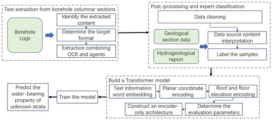
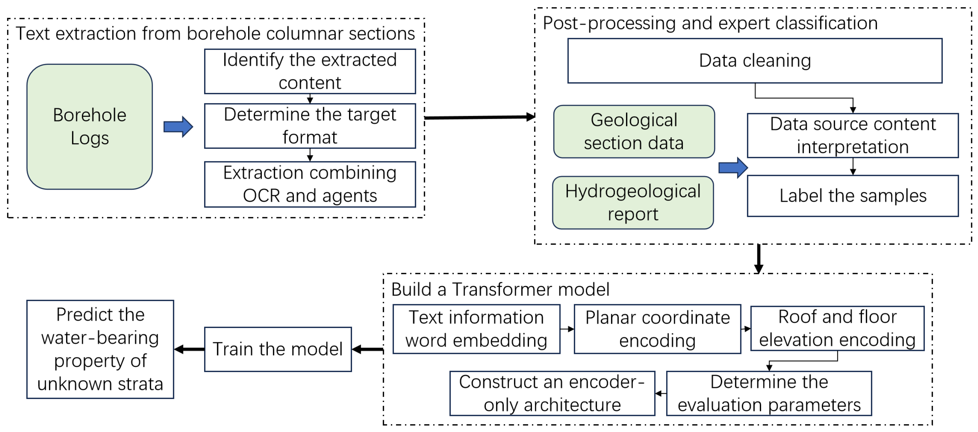
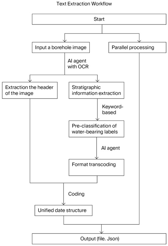
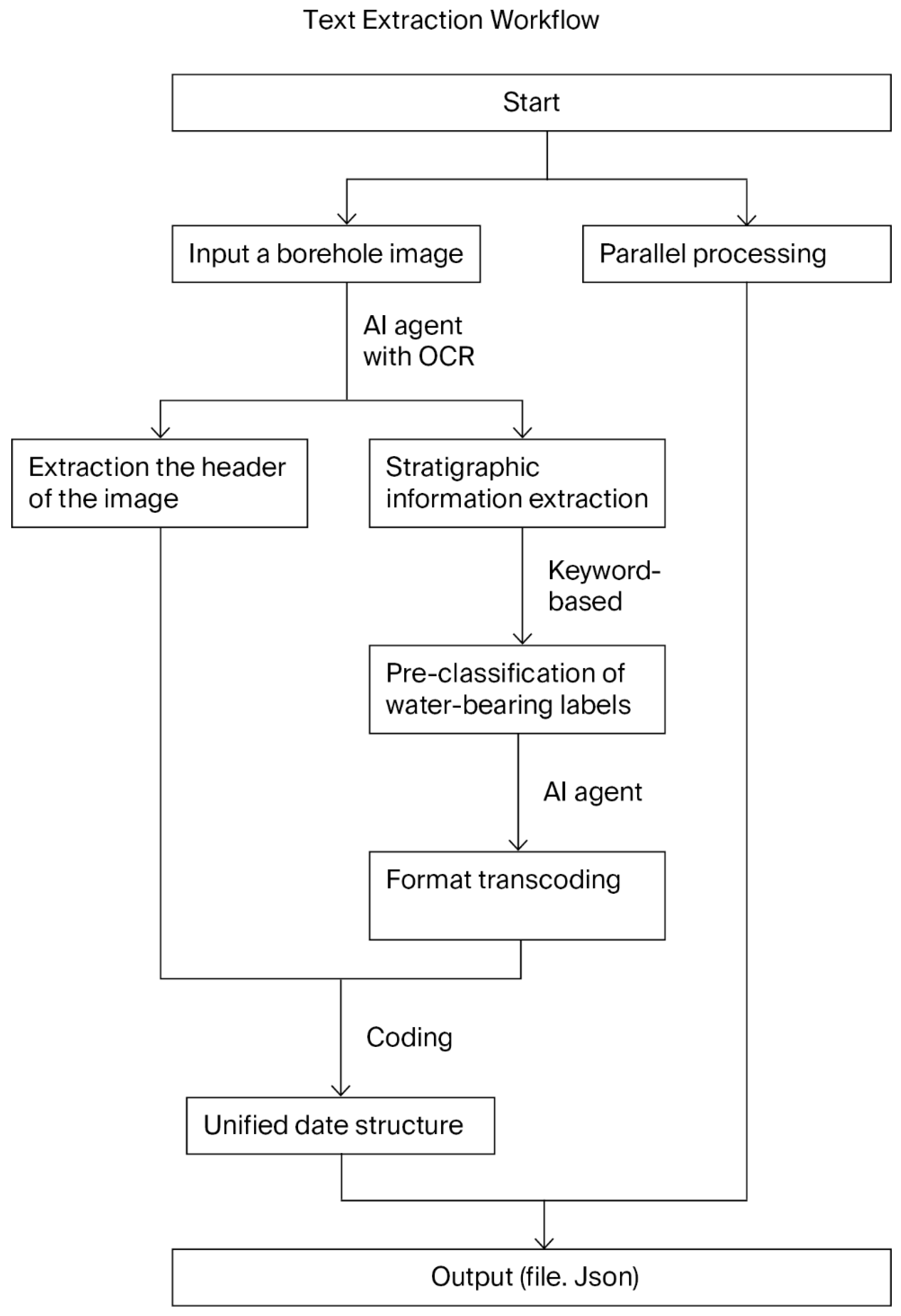
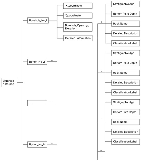
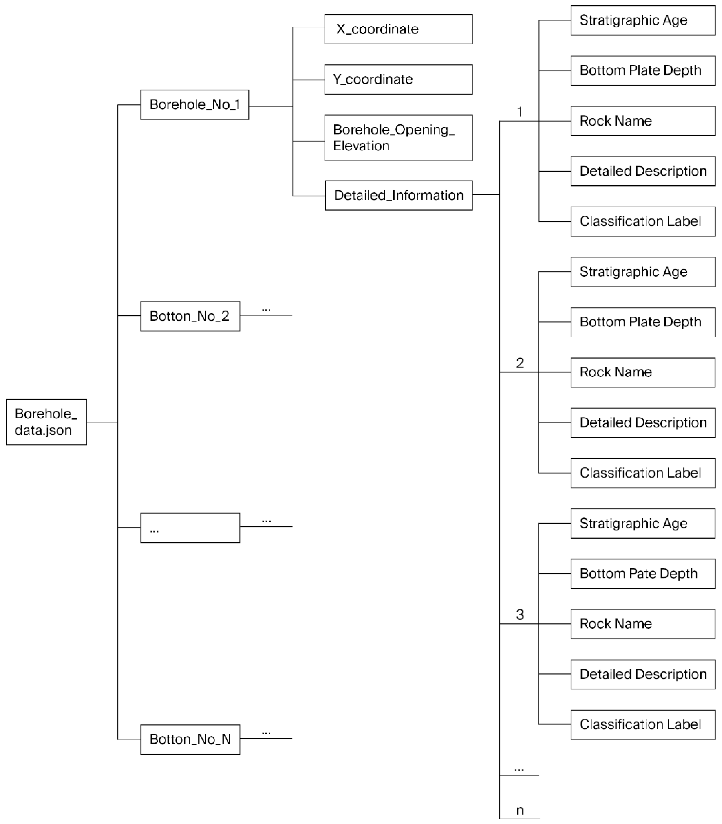
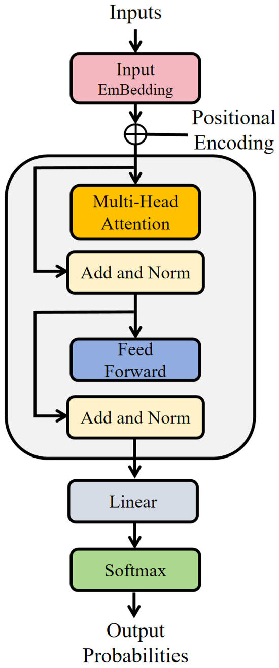
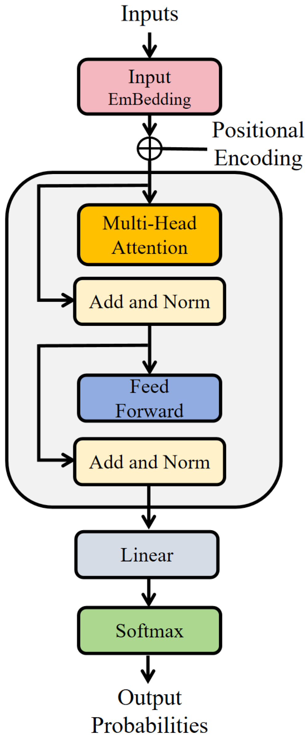
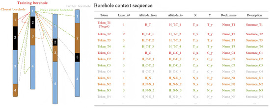
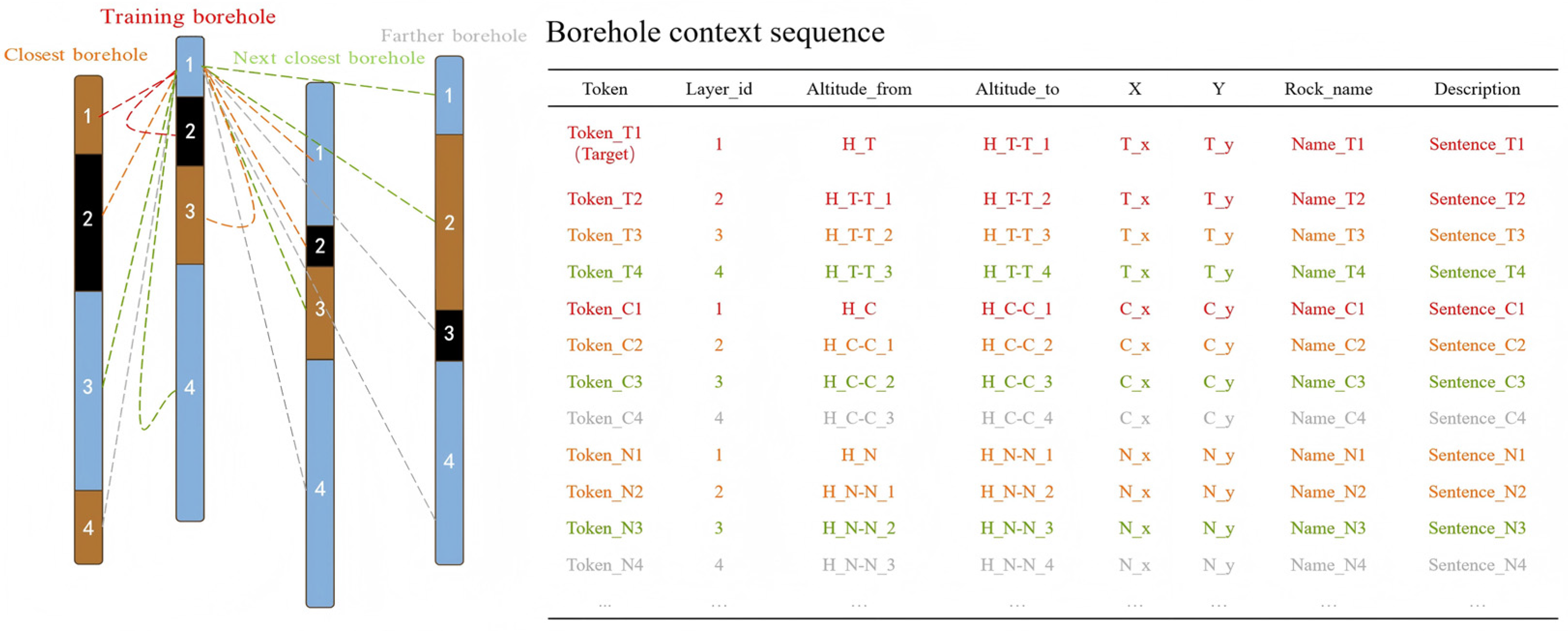
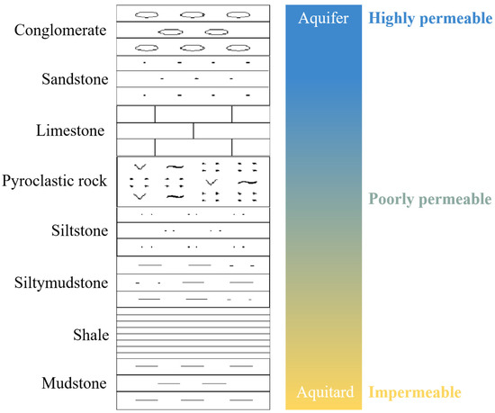
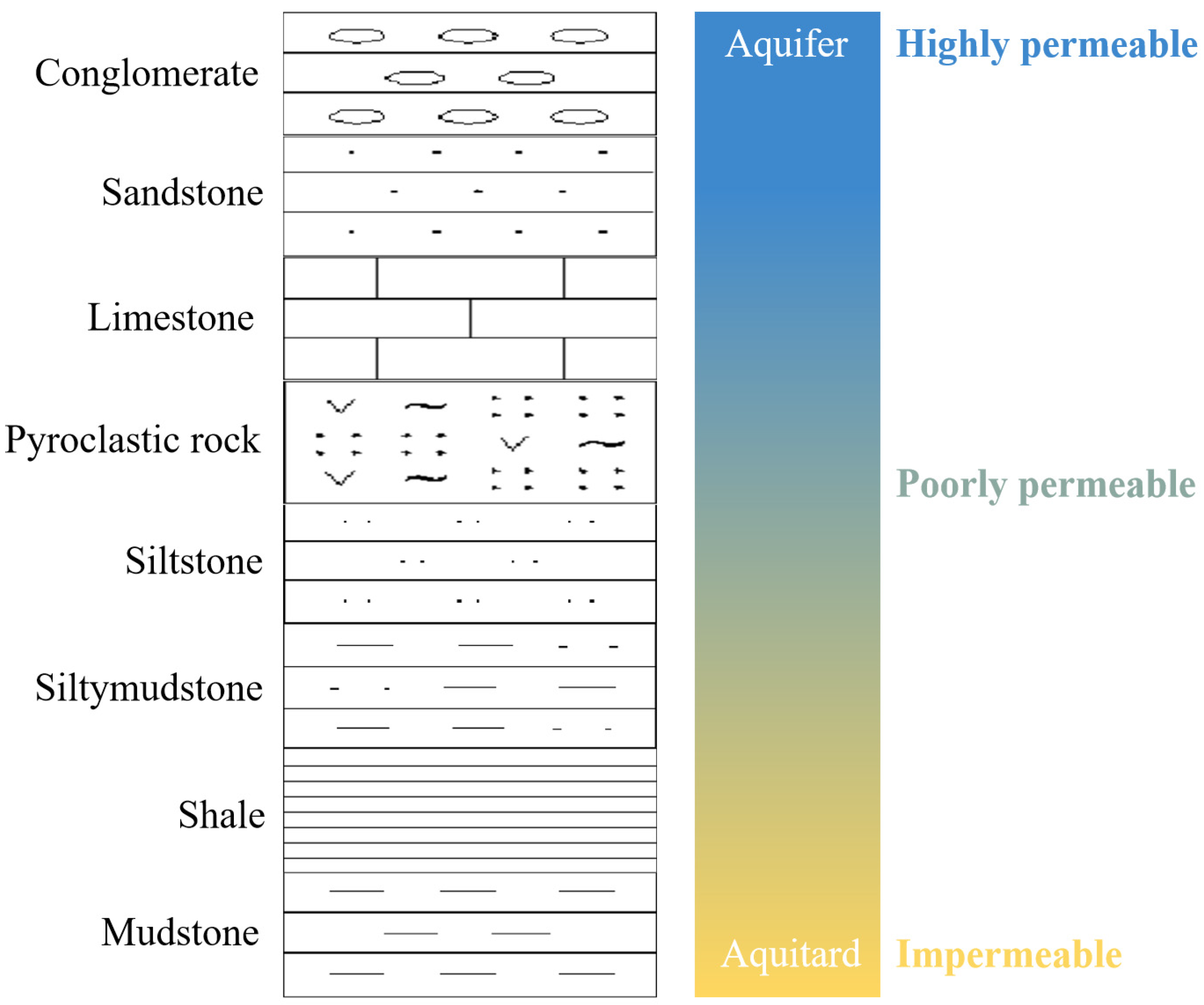
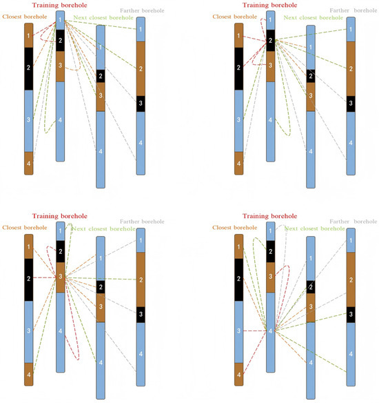
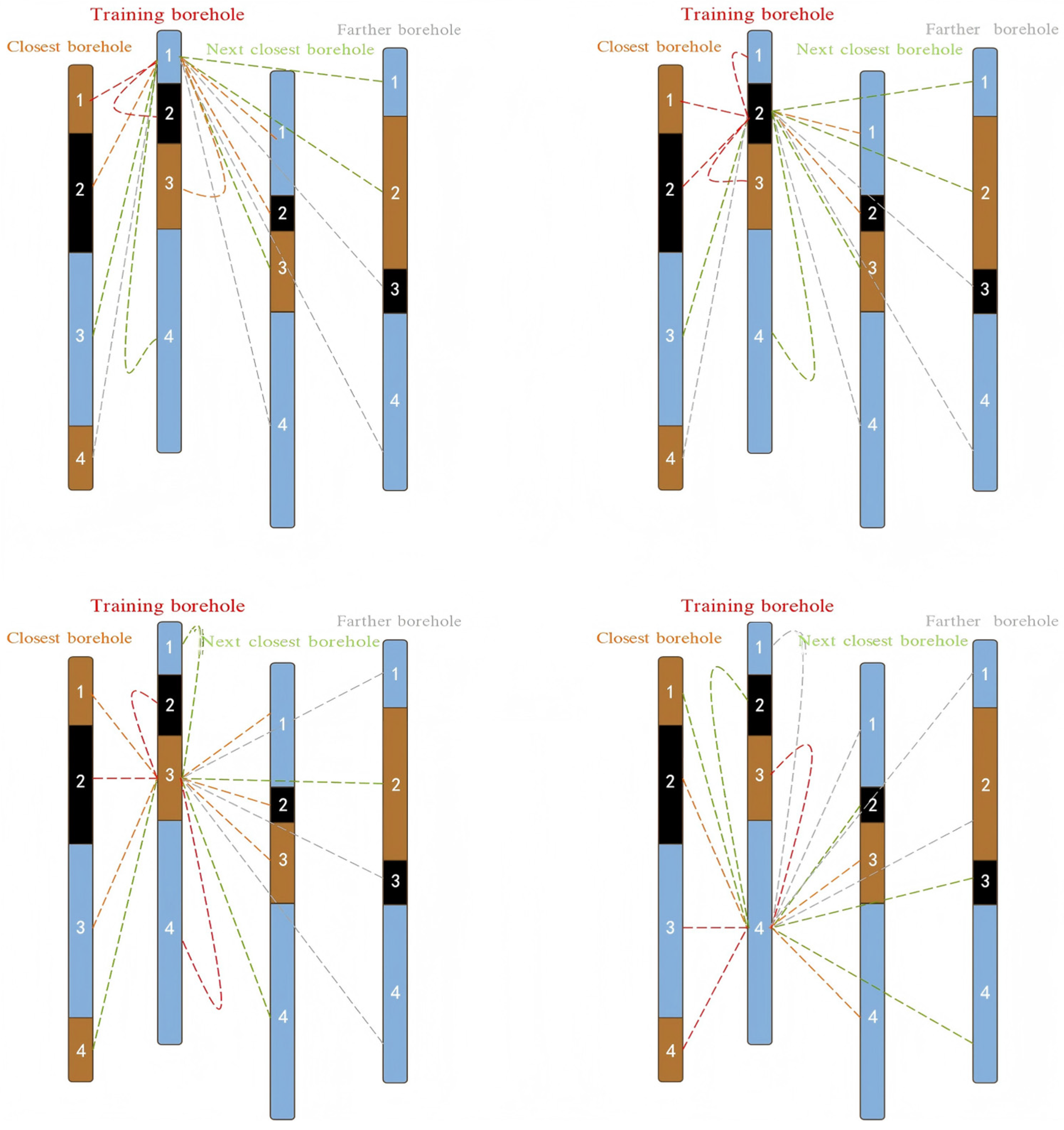
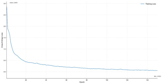
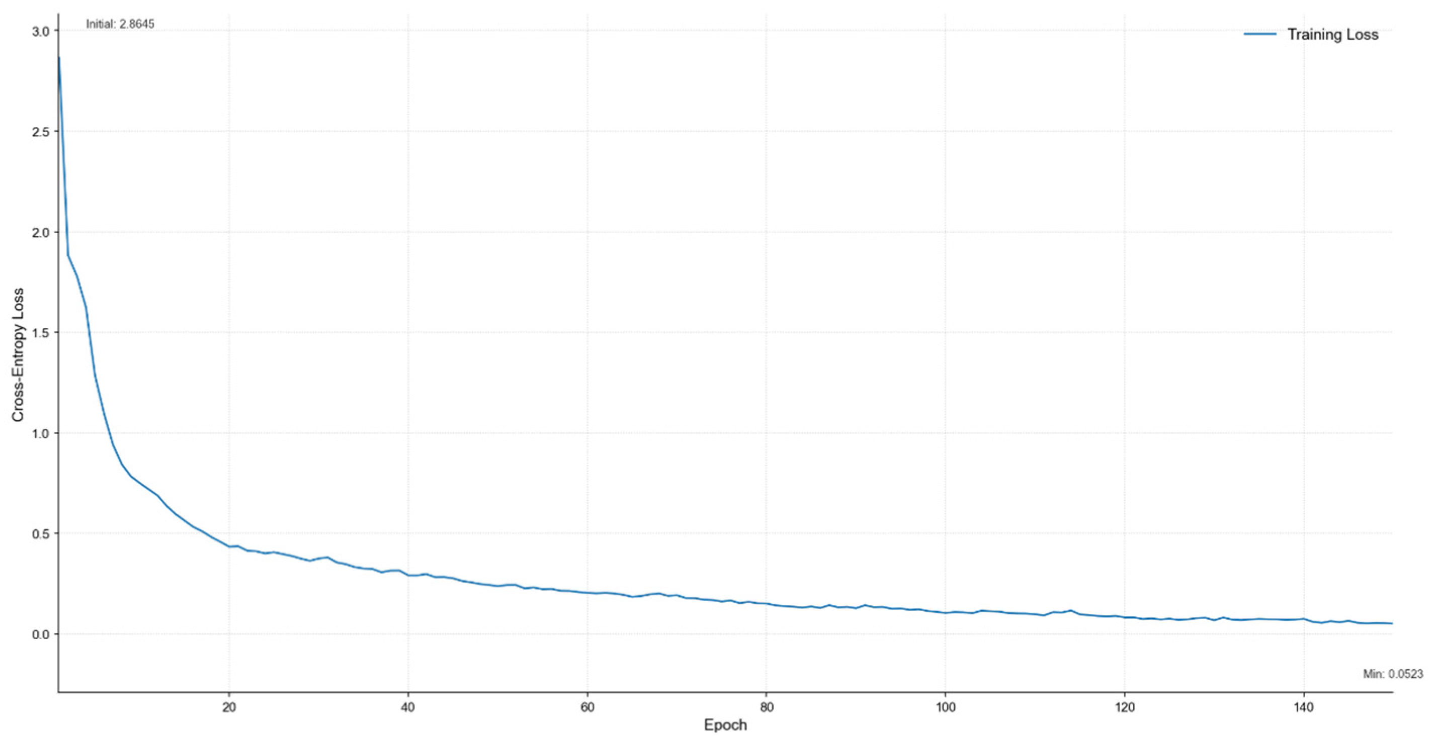
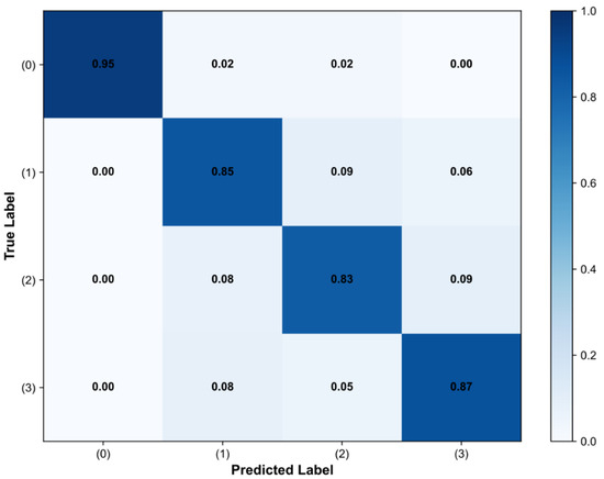
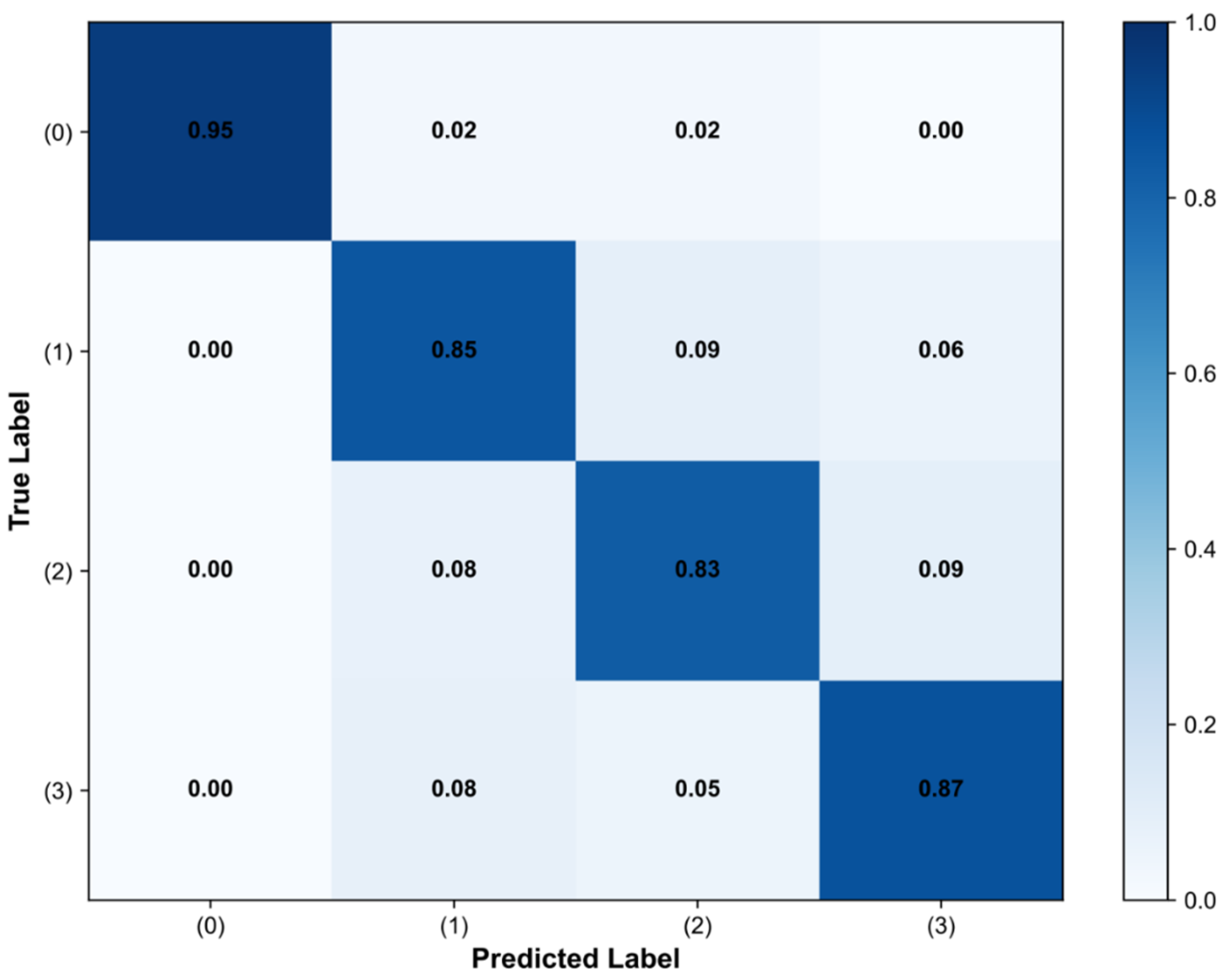
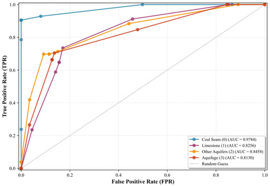
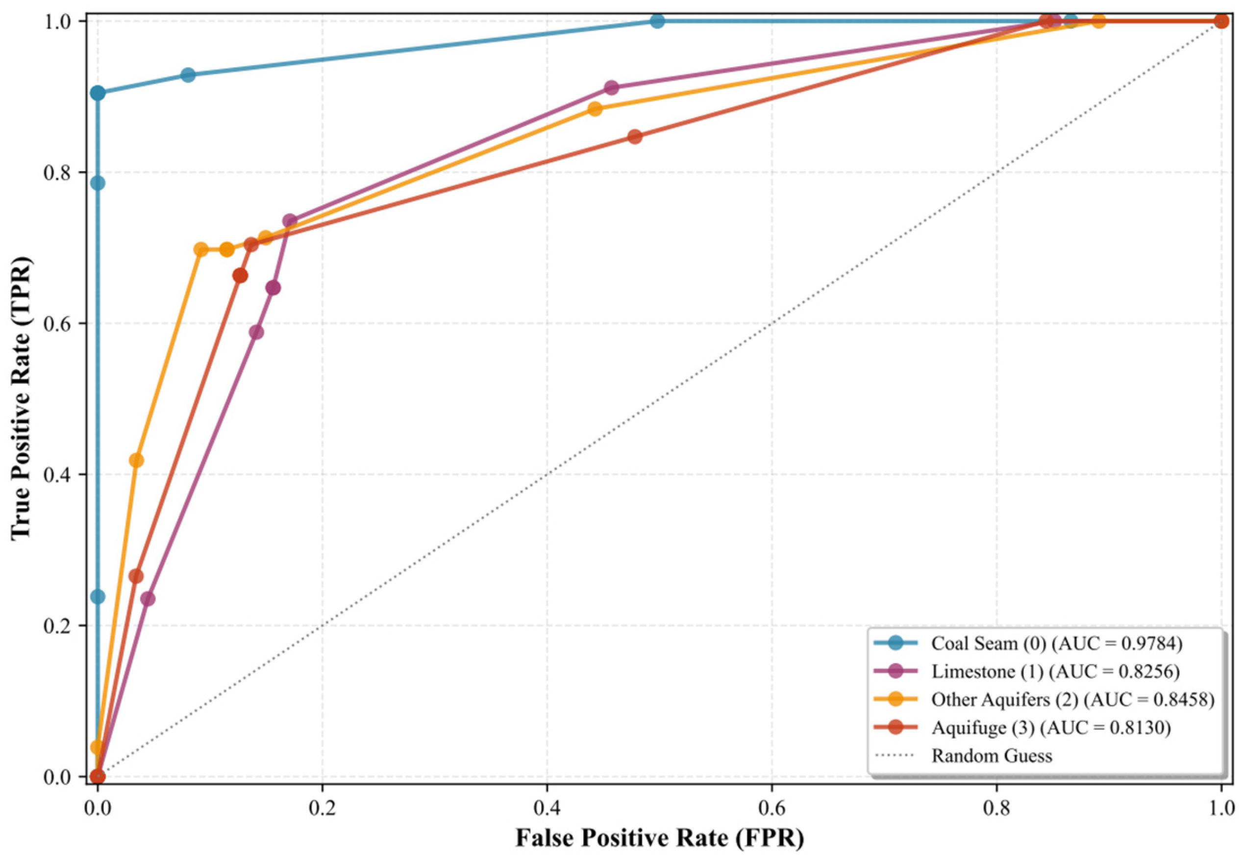
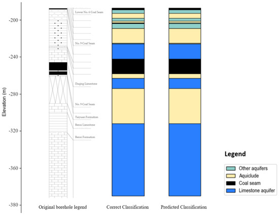
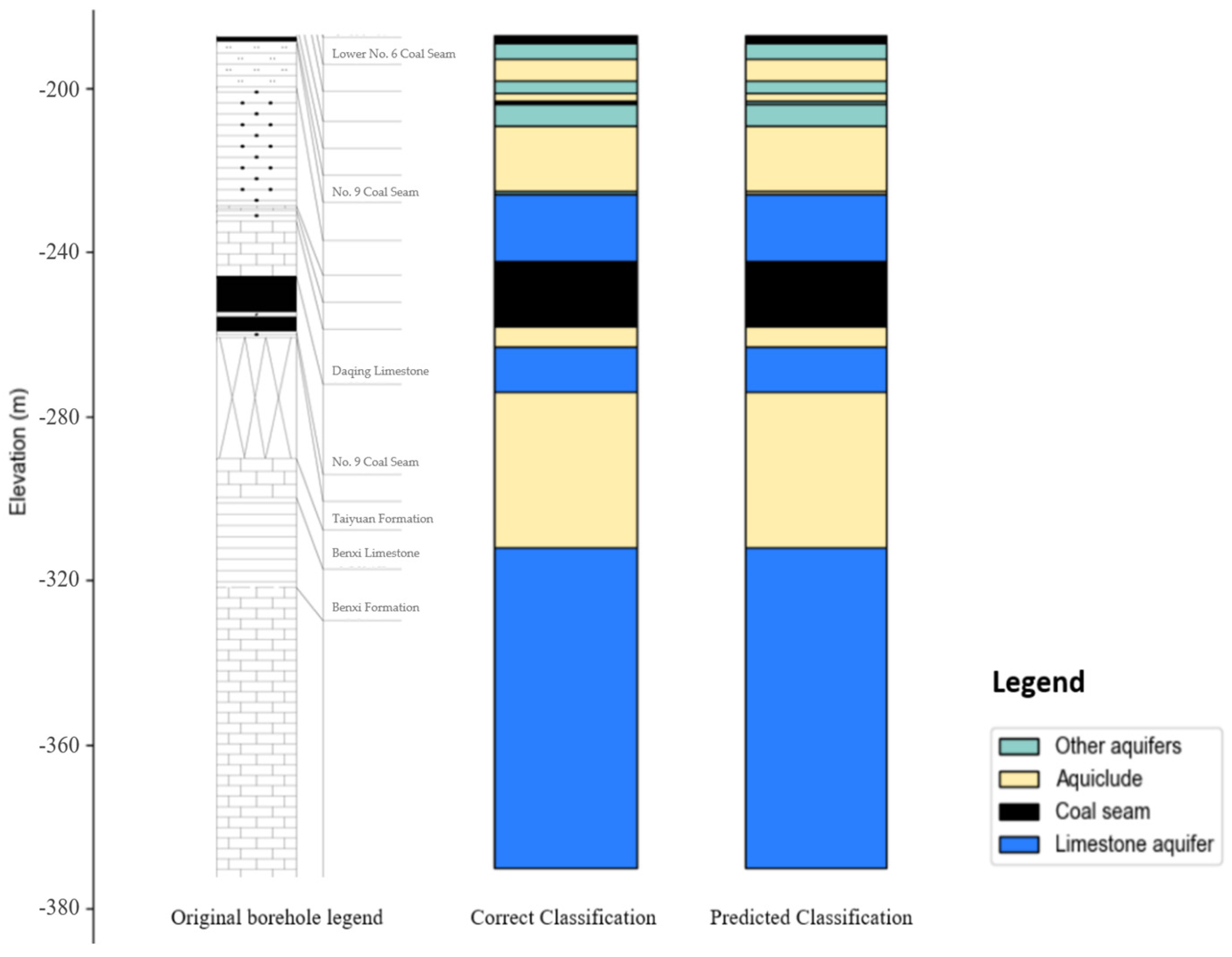
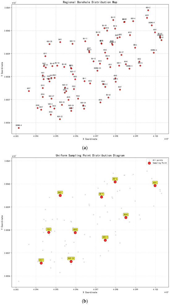
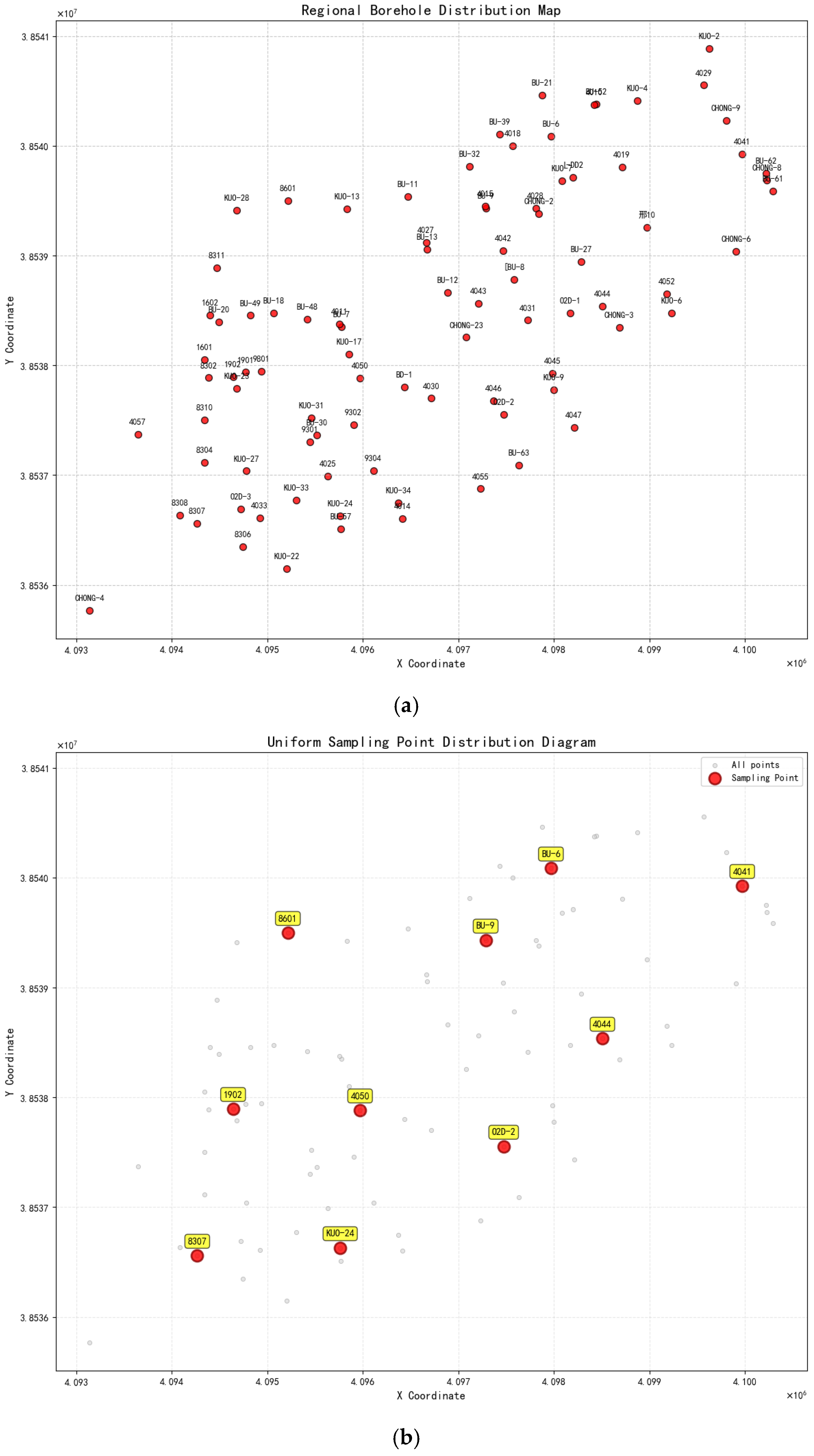
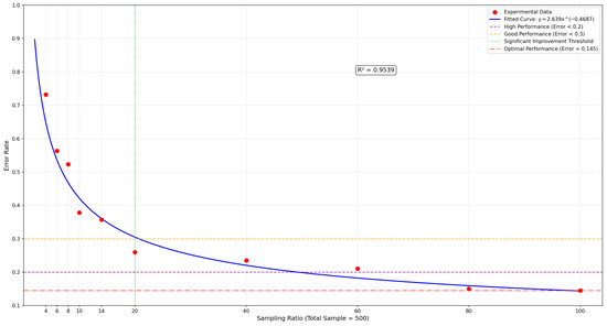
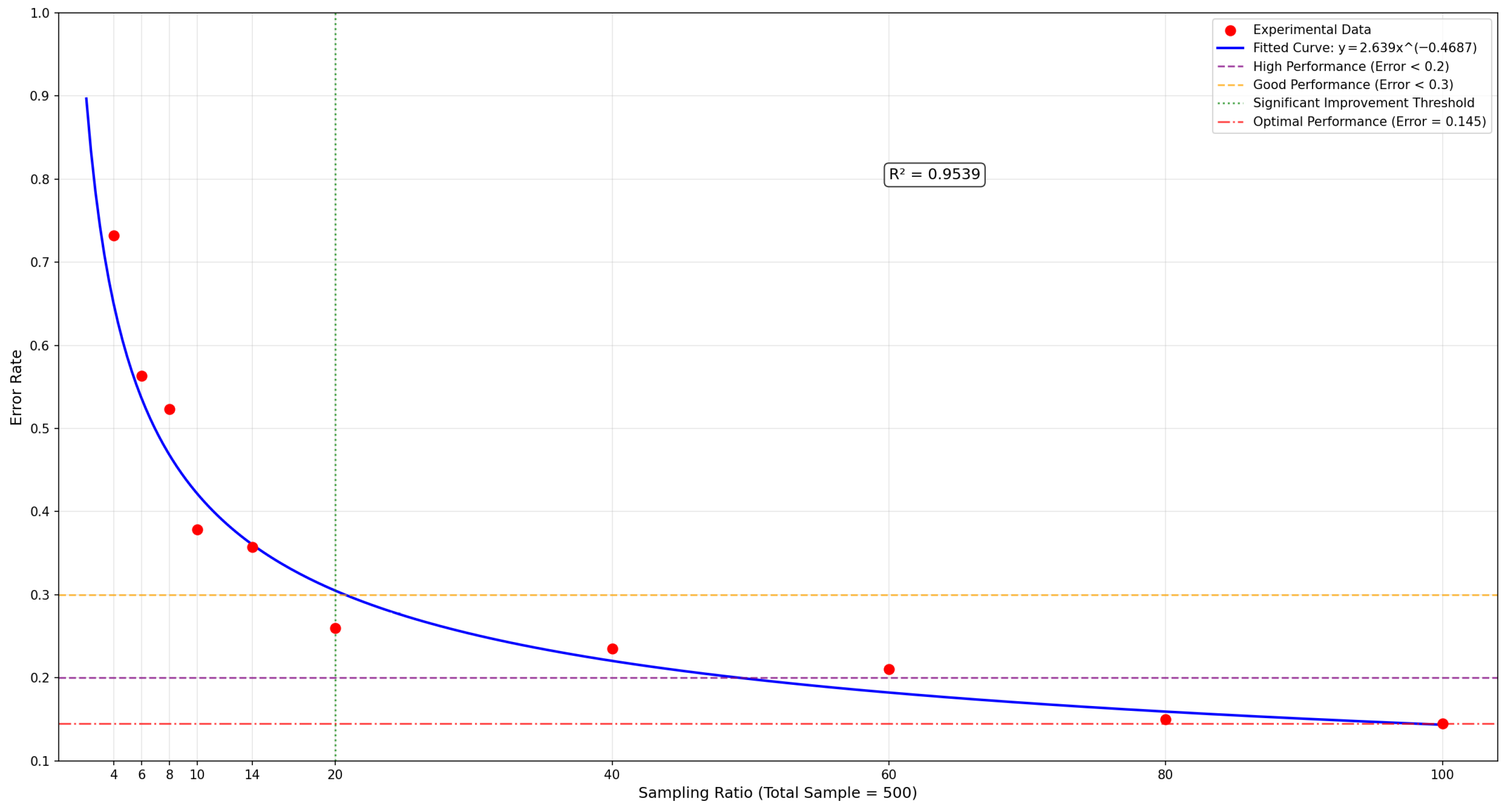
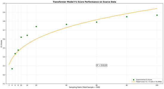
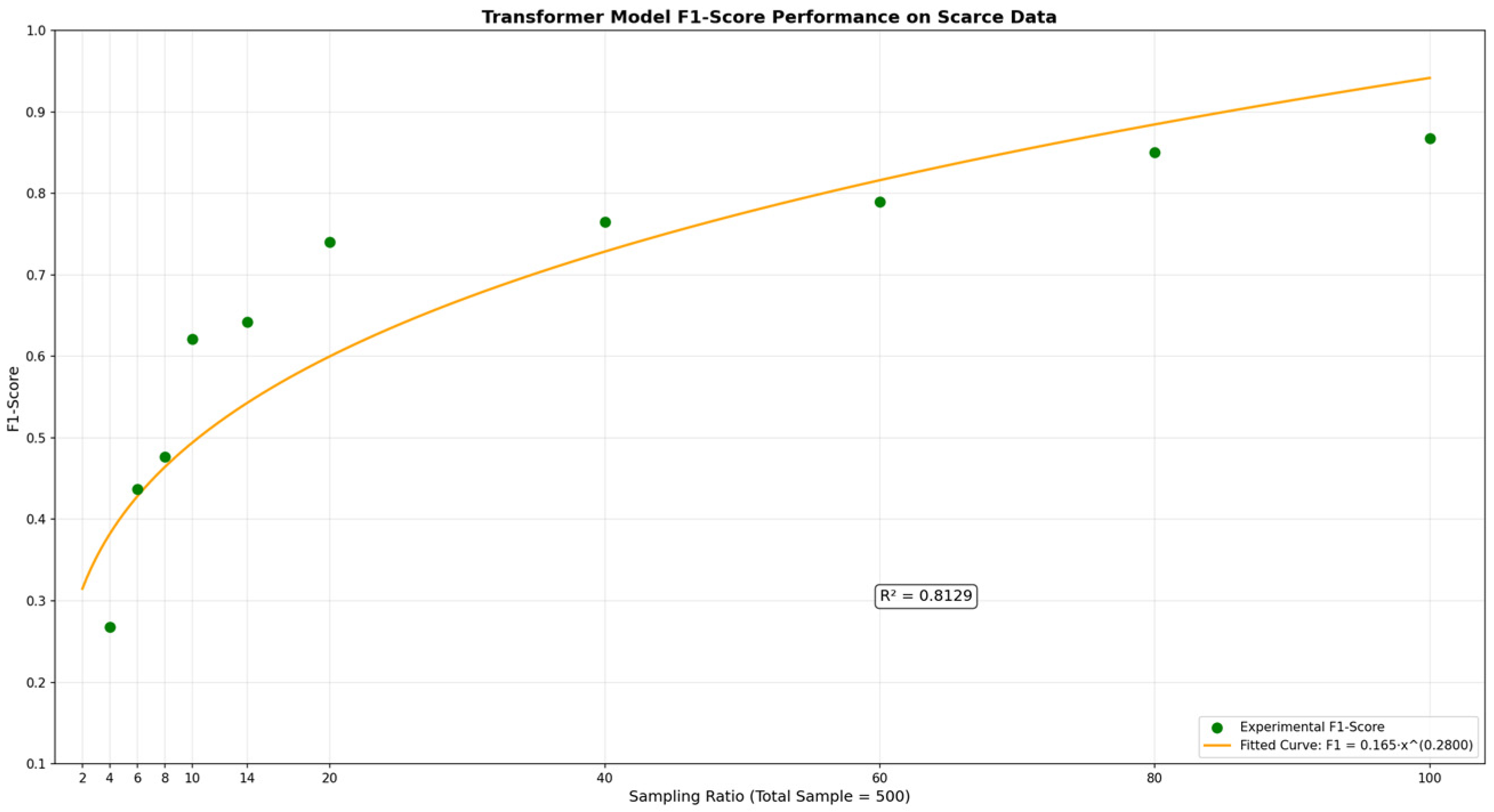
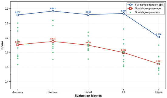
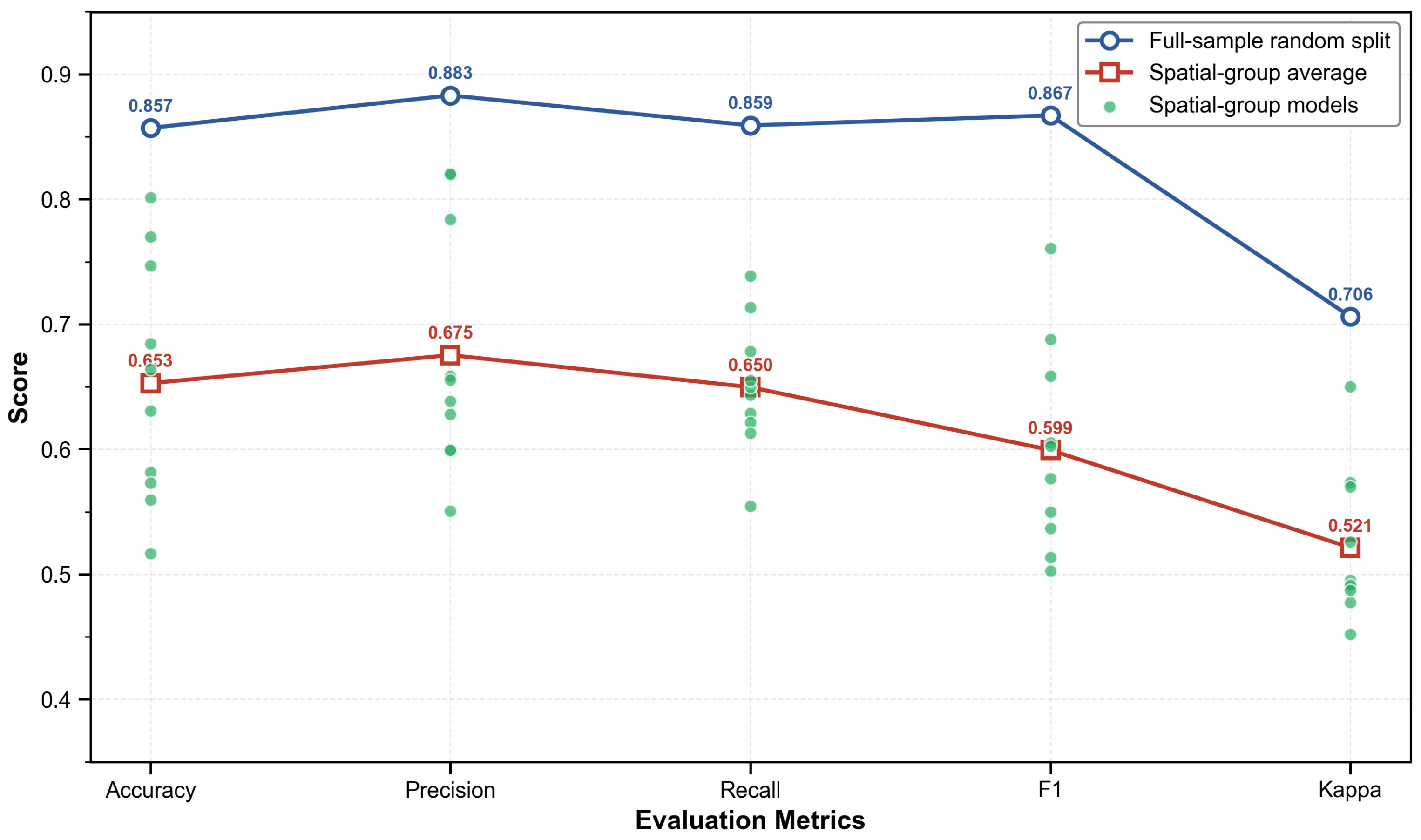
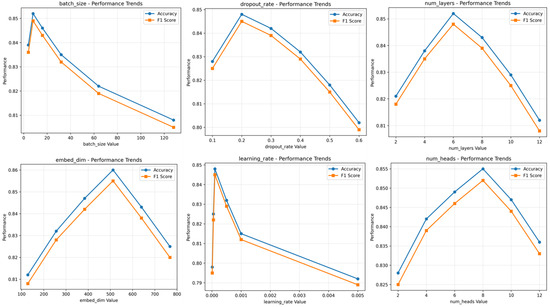
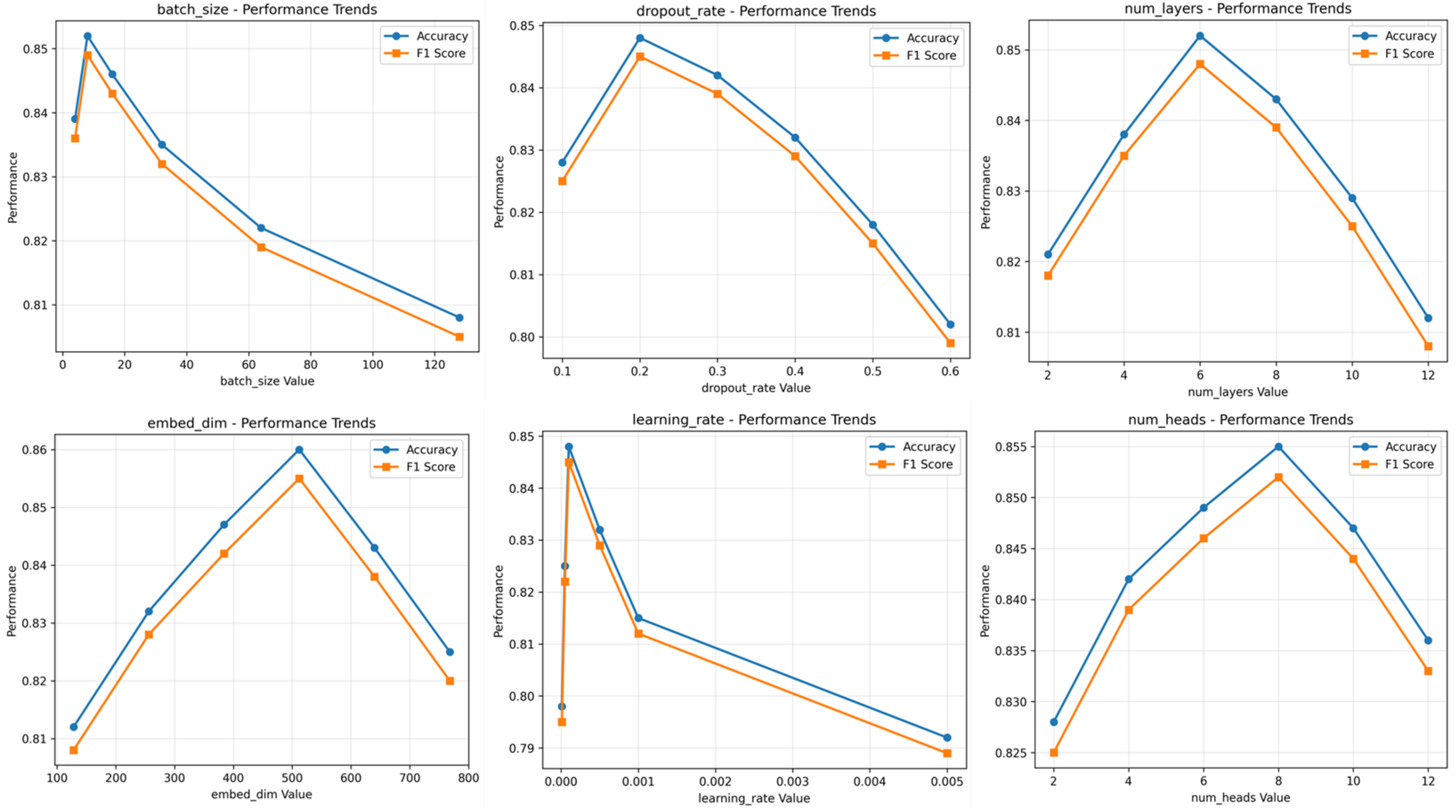
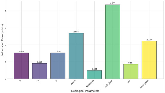
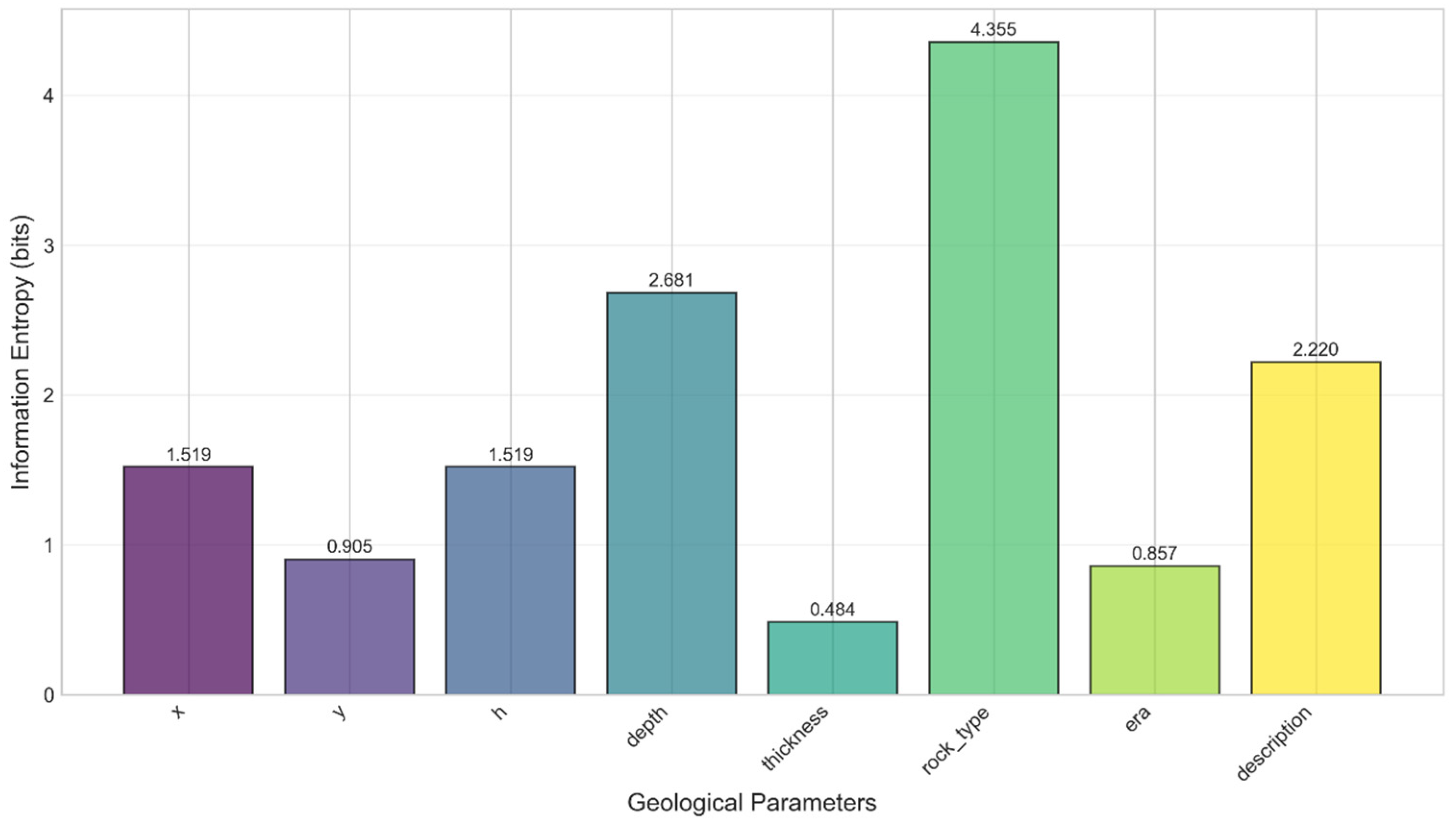
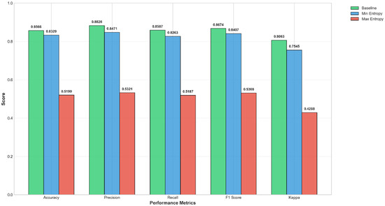
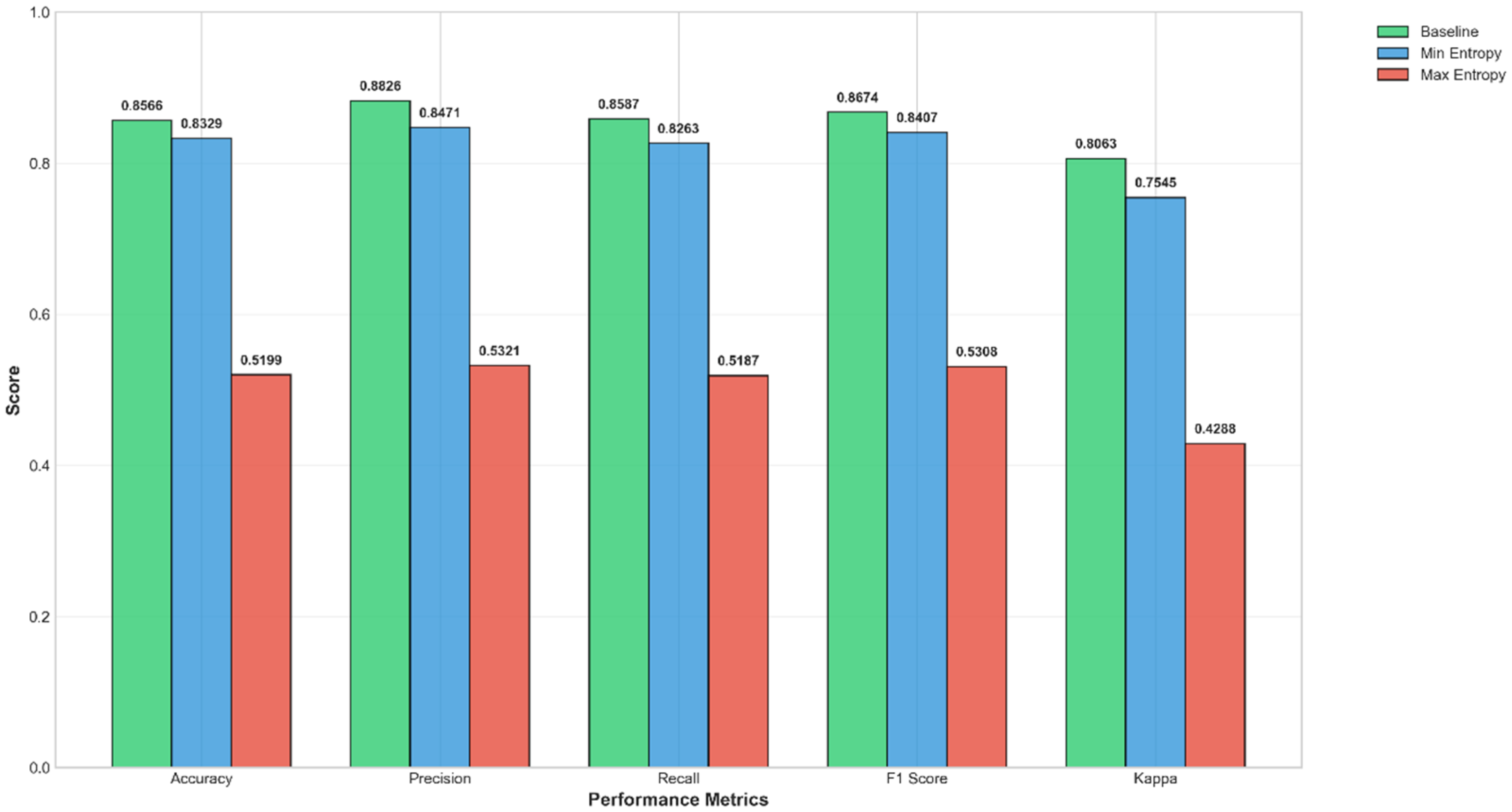

Disclaimer/Publisher’s Note: The statements, opinions and data contained in all publications are solely those of the individual author(s) and contributor(s) and not of MDPI and/or the editor(s). MDPI and/or the editor(s) disclaim responsibility for any injury to people or property resulting from any ideas, methods, instructions or products referred to in the content. |
© 2026 by the authors. Licensee MDPI, Basel, Switzerland. This article is an open access article distributed under the terms and conditions of the Creative Commons Attribution (CC BY) license.