Modeling CO₂ Emissions of a Gasoline-Powered Passenger Vehicle Using Multiple Regression

Abstract

The article presents issues related to fossil fuel energy consumption and CO₂ emissions from motor vehicles. It identifies the main areas of research in this field in the context of motor vehicles, namely driver behavior, fuel consumption, and OBD systems. The research sample consisted of experimental data containing records of a series of test drives conducted with a passenger vehicle equipped with a gasoline-powered internal combustion engine, collected via an OBD diagnostic interface. Three subsets related to engine operation and energy demand patterns were distinguished for the study: during vehicle start-up and low-speed driving (vehicle start-up mode), during urban driving, and during extra-urban driving. Multiple regression models were constructed for the analyzed subsets to predict CO₂ emissions based on engine energy output parameters (power, load) and vehicle kinematic parameters. The developed models were subjected to detailed evaluation and mutual comparison, taking into account their predictive performance and the interpretability of the results. The analysis made it possible to identify the variables with the most substantial impact on CO₂ emissions and fuel energy consumption. The models allow individual drivers to monitor and optimize vehicle energy efficiency in real-time. The extra-urban driving model achieved the highest predictive accuracy, with a mean absolute error (MAE) of 19.62 g/km, which makes it suitable for real-time emission monitoring during highway driving.

1. Introduction

The ongoing transformation of the transport sector toward a low-emission economy, along with increasingly stringent environmental protection regulations, makes precise monitoring of carbon dioxide (CO₂) emissions from passenger vehicles increasingly important both at the systemic and individual levels [1,2]. Existing strategies aimed at reducing the negative impact of the automotive sector on the climate have primarily focused on vehicle manufacturers and the implementation of new type-approval standards. However, the role of the end user is equally significant, as greater awareness of one’s own environmental impact can lead to more responsible operational and purchasing decisions.

Modern passenger vehicles are equipped with advanced On-Board Diagnostics (OBD) systems that enable continuous real-time recording of technical parameters, including data related to fuel consumption and emission levels. The availability of such data makes it possible to develop mathematical models that can predict actual CO₂ emissions based on real operating conditions. Particularly promising in this regard is the use of multiple regression methods, which make it possible to consider many explanatory variables simultaneously, thereby improving the accuracy and reliability of estimation [3]. Using OBD data as an input source for regression models represents an important step toward the personalization of assessing the environmental impact of an individual passenger vehicle user.

1.1. Emission Issues in the Context of the European Union

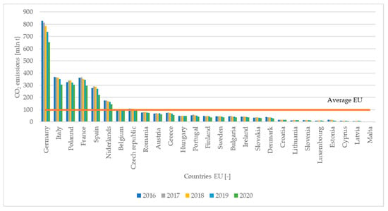
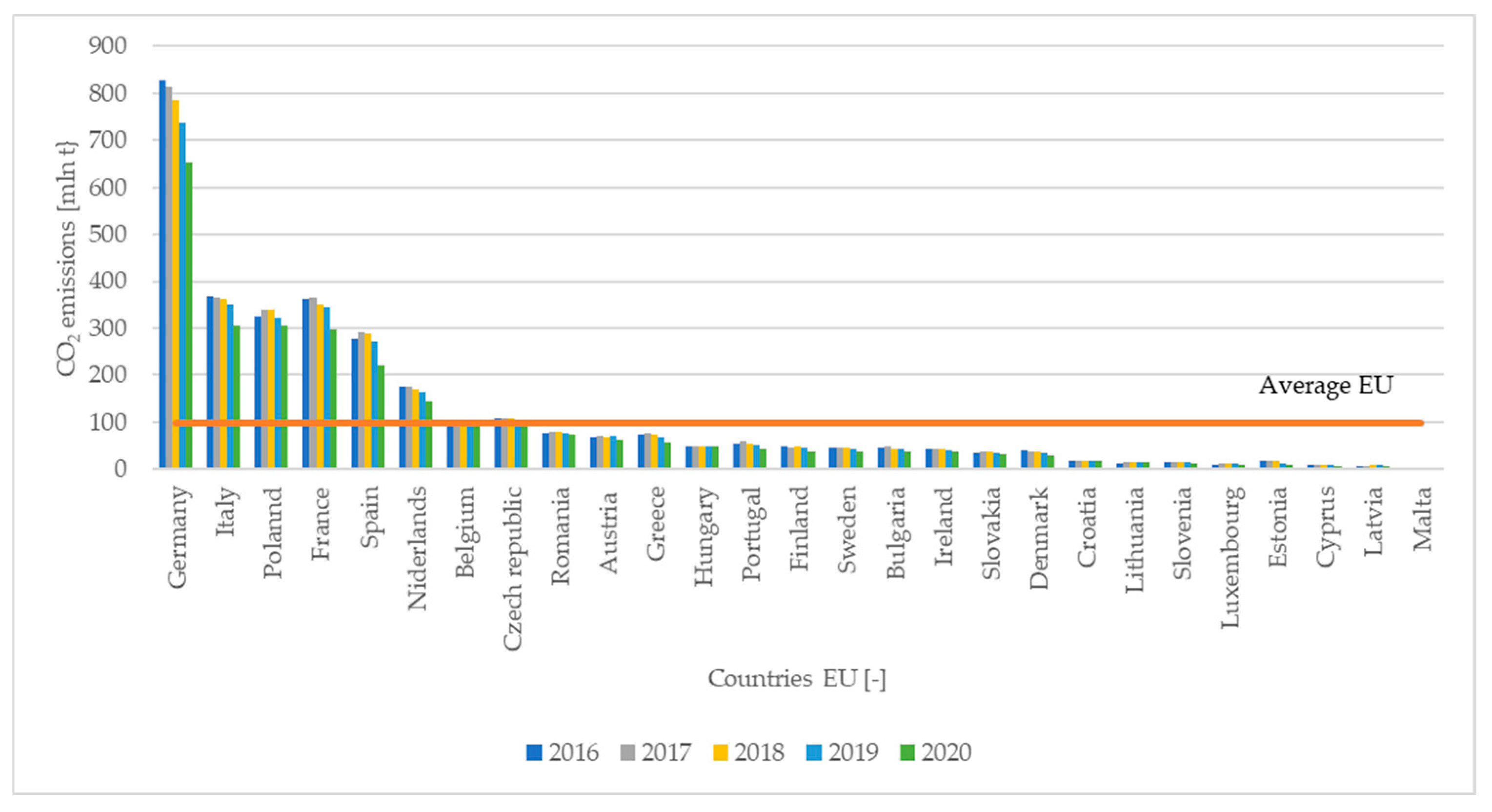
The reduction in harmful emissions from motor vehicles is currently one of the most significant environmental challenges observed within the European Union (EU), obligating member states to take action in this area [4]. The requirements concern greenhouse gas emissions, including carbon dioxide (CO₂), methane (CH₄), and nitrous oxide (N₂O) [5,6]. Figure 1 presents emission levels between 2016 and 2020 across EU member states. It can be observed that Germany is the largest CO₂ emitter within the European Union, while Poland ranks third, producing three times more CO₂ than the 10-year EU average (119.3 million tons).

Figure 1. CO₂ Emissions in European Union Countries in 2016–2020.

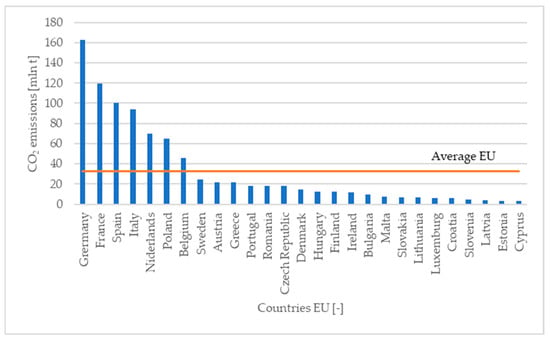
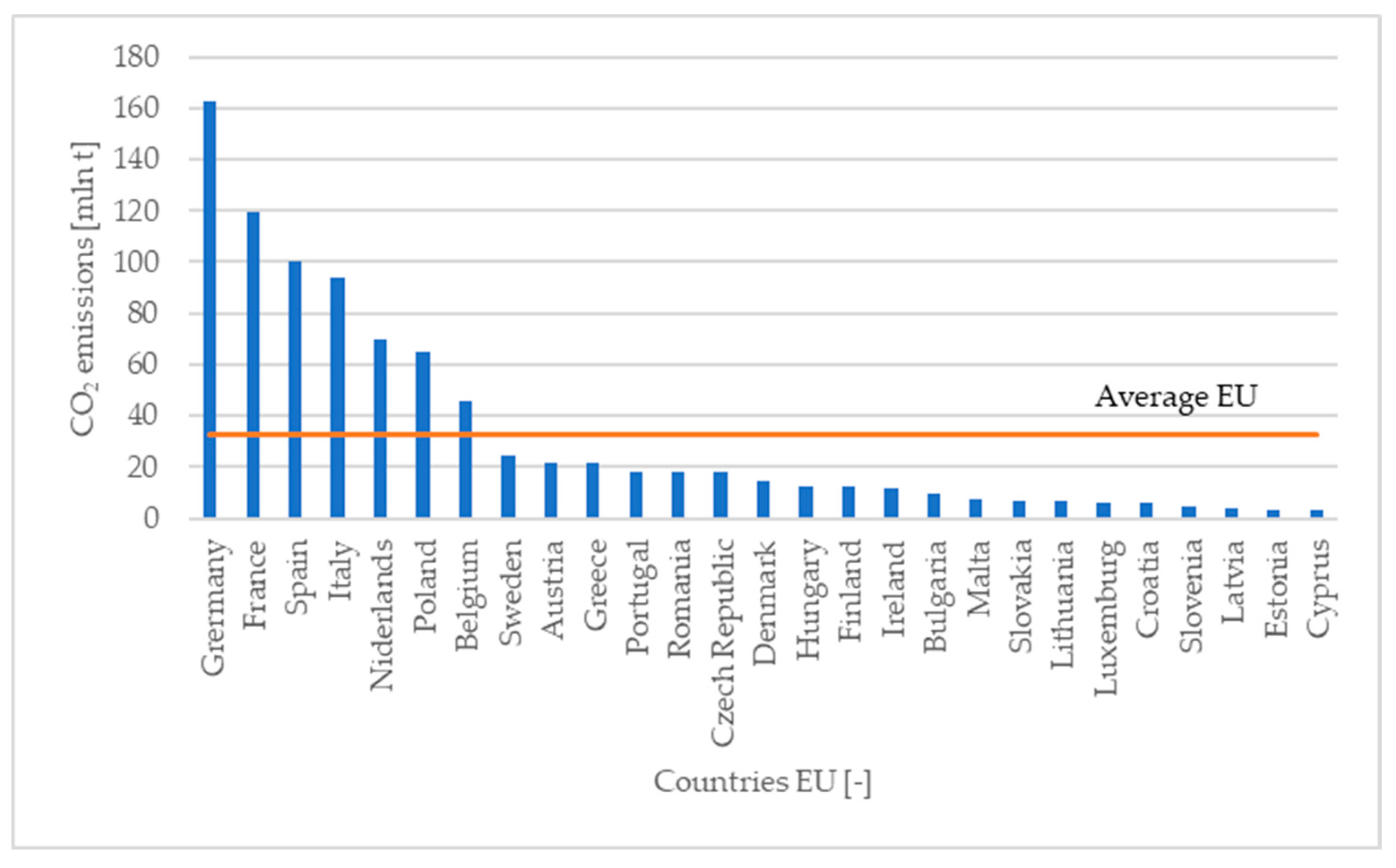
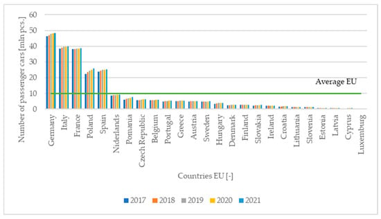
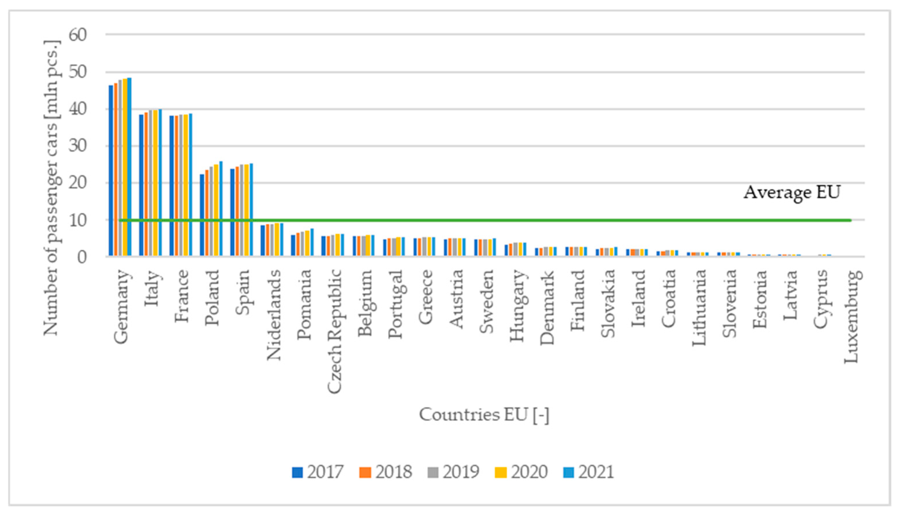
The European Union recognizes the transport sector as one of the areas of the economy with the most harmful impact on the natural environment and human health, as it plays a significant role in shaping CO₂ emission levels within the EU, accounting for approximately 30% of total CO₂ emissions (Figure 2). About 70% of this amount originates from road transport, with passenger cars generating as much as 61% of it [5]. The number of registered motor vehicles was also analyzed. In 2021, there were approximately 250 million vehicles across the European Union, 19% of which were in Germany (48.54 million). Poland ranked fourth, with a total of 25.87 million vehicles (10%) (Figure 3). The average number of vehicles per country in Europe is about 10 million. It can be observed that around 3.7 million new vehicles are added annually across the European Union. In Poland the annual increase amounts to about 850,000 vehicles.

Figure 2. CO₂ emissions from transport in European Union countries in 2020.

Figure 3. Number of passenger cars in the EU in 2017–2021.

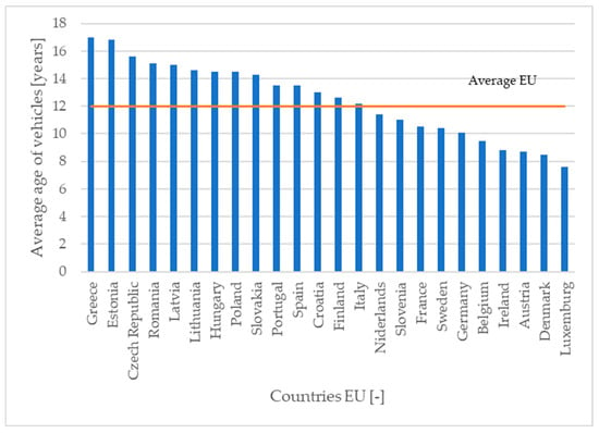
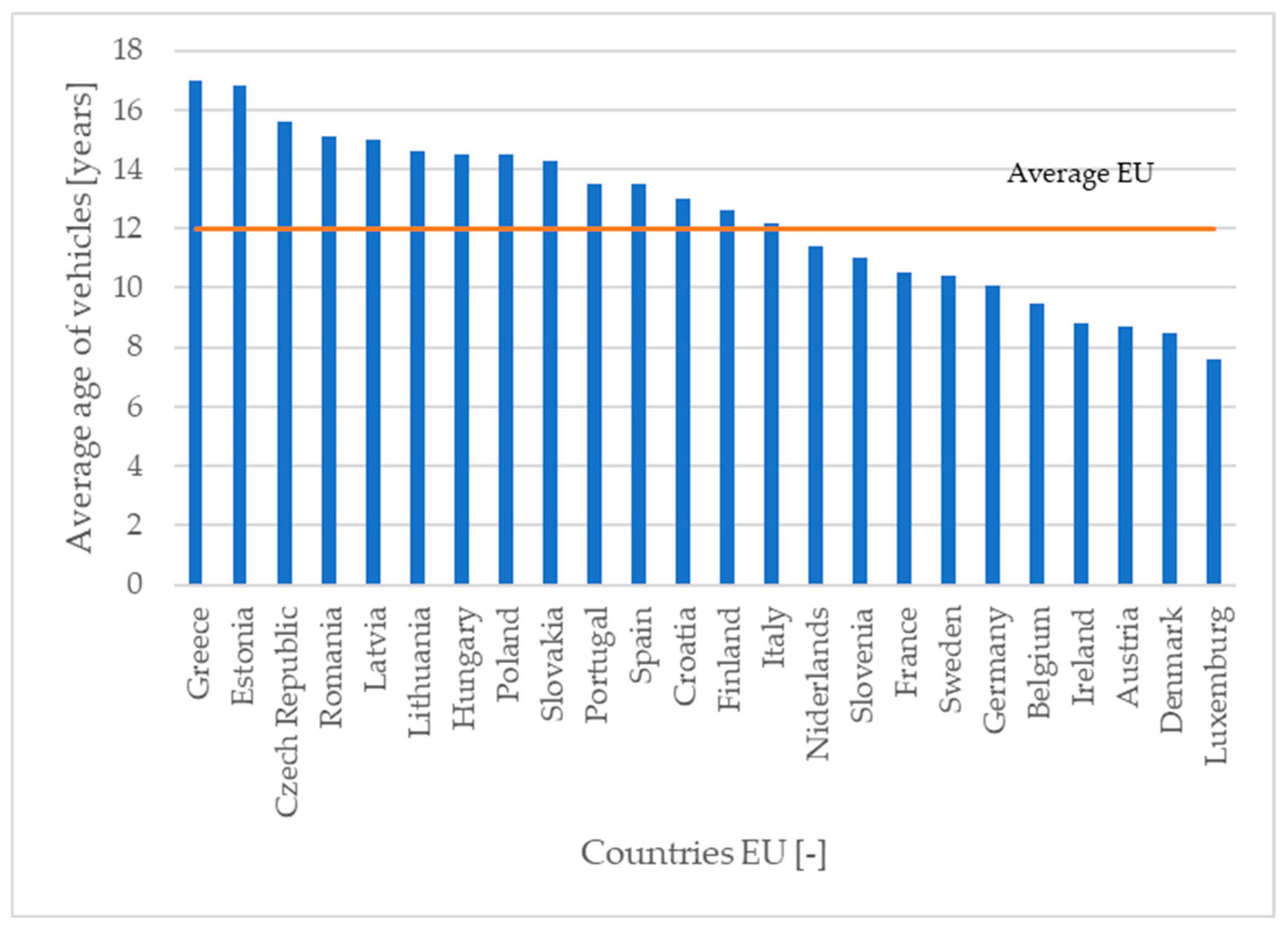
An important factor is also the average age of vehicles. Figure 4 presents the results for individual EU countries in 2021. The oldest vehicles are found in Greece (17 years), while the newest are in Luxembourg (7.6 years). The EU average vehicle age is 12 years, while Poland ranks eighth, with an average vehicle age of 14.5 years.

Figure 4. Average Vehicle Age in the EU in 2021.

Another key aspect is the share of vehicles over 10 years old in European Union countries. According to 2021 data, the country with the highest proportion of vehicles older than 10 years is Romania, with 87% (6.5 million vehicles). Greece ranks second, with 84% (4.5 million vehicles). Poland ranks third with 81% of vehicles (approximately 21 million) that are more than 10 years old. This is largely due to the fact that many vehicles operating on Polish roads are imported from other EU countries, and only about 1.3 million of them are under 3 years old [7]. Luxembourg and Ireland have the lowest shares of vehicles in this age category, at 25% and 37%, respectively.

Another important factor is the type of vehicle powertrain. According to the 2023 ACEA Vehicles in Use report [8], approximately 51.1% of all passenger cars in the European Union are powered by gasoline. Diesel accounts for about 41.9% of vehicles, LPG for 2.5%, while hybrid electric vehicles (HEV) make up 2.3%. Battery electric vehicles (BEV) represent only 0.8%, and plug-in hybrid electric vehicles (PHEV) account for 0.7%.

For this reason, the EU has introduced regulations aimed at reducing these emissions. The EU policy in this area focuses, among other measures, on introducing new and increasingly stringent CO₂ emission standards for new passenger cars. These standards are ultimately intended to achieve climate neutrality by 2050 and a 90% reduction in transport-related emissions. Although these actions are global in scope, certain local initiatives can also contribute to reducing CO₂ emissions. One of the key measures is increasing driver awareness of eco-driving principles. Effective transport decarbonization requires not only systemic changes but also operational-level actions focused on individual users. Individual driving habits—such as smooth driving, avoiding excessive acceleration and braking, and efficient fuel use—can have a significant impact on total greenhouse gas emissions. In order for educational and motivational strategies at the individual level to produce tangible global effects, it is necessary to provide drivers with appropriate tools to support their decision-making processes. One such tool may be mathematical models developed on the basis of data obtained from the On-Board Diagnostic (OBD) system, which accurately analyze the influence of various factors—such as driving style, vehicle load, and road conditions—on CO₂ emissions. Such measures are particularly important given the continuously increasing number of vehicles in the European Union. In this context, the present study undertook research aimed at developing a model for assessing the formation of CO₂ emission levels using a selected vehicle as an example, focusing on the level of an individual road user.

Based on the literature review, it was determined that the most significant factors in the context of modeling vehicle emissions can be grouped into three thematic areas: driving style, fuel consumption, and diagnostic systems.

An analysis of the literature concerning driving style has shown that driver behavior on the road can significantly contribute to reducing the carbon footprint associated with road transport. Key aspects in this area include vehicle speed and driving dynamics.

Another thematic area is fuel consumption, which is directly linked to CO₂ emissions. A review of the literature in this field has shown that a number of forecasting methods are used in fuel consumption modeling, such as linear regression, decision trees, and neural networks. A very important issue in this area is the identification of vehicle-related factors (engine operating parameters, vehicle kinematic parameters, etc.) that directly affect fuel consumption. The literature review indicates that significant influencing factors include, among others, vehicle speed, engine rotational speed, engine load, and engine power.

The driver’s role is also crucial in the context of vehicle emissions [9]. Therefore, the ability to diagnose driving style is particularly important for identifying—and ultimately eliminating—“negative” and “positive” driver behaviors. The “positive” driving style involves smooth acceleration, maintaining constant moderate speeds, and minimizing throttle variations. The “negative” (aggressive) style features rapid acceleration, frequent high-load operation, and variable speed patterns, resulting in higher CO₂ emissions. The collection, analysis, and evaluation of such information may make it possible to identify advanced patterns and determine the influence of selected factors on vehicle emission levels.

1.2. Literature Review on CO₂ Emission Modeling

CO₂ emission in motor vehicles is a complex issue that depends on numerous influencing factors. Their correct identification is essential for the development and implementation of CO₂ emission reduction strategies, particularly to meet the need for a deeper understanding, analysis, and assessment of the influence of individual variables on CO₂ emissions. Therefore—based on a review of the literature—the most significant of these factors were identified, including, in addition to CO₂ emission measurement methods [10]:

• The type of fuel used to power the vehicle [11];
• The driver’s driving style [12,13,14,15];
• The amount of fuel consumed [10,11,14,16];
• The share of electrical energy consumers in vehicles that affect driving comfort and performance, the so-called functional systems [16];
• Kinematic parameters characterizing vehicle motion, such as speed and acceleration [11,14,15];
• And the diagnostic systems used [17,18].

Modern internal combustion engines in passenger vehicles are mainly powered by gasoline or diesel fuel. An analysis of CO₂ emissions and fuel consumption data for selected combustion vehicles can be found, among others, in [19]. That study also described the differences in CO₂ emission regulations across different countries and, based on the collected data on CO₂ emissions and fuel consumption, compared them with theoretical stoichiometric calculations of CO₂ emissions derived from fuel combustion reactions. A linear regression model was used for this purpose, and the obtained results showed that compression-ignition (diesel) engines, despite lower fuel consumption, emit more CO₂ per unit of distance traveled compared to spark-ignition (gasoline) engines.

The issue of vehicle manufacturers adapting to the applicable CO₂ emission standards depends on the ability to accurately measure, among other things, fuel consumption levels and CO₂ emissions under typical operating conditions of a vehicle [20,21]. Due to the need to ensure the repeatability of results, such measurements are carried out under laboratory conditions, which may lead to significant discrepancies between laboratory measurements and those obtained during real-world vehicle operation. The article [10] provides an overview of the causes of differences between measured fuel consumption in laboratory conditions and in real use, as well as CO₂ emissions from passenger cars operated in Europe.

The driver is another key factor that must be taken into account when analyzing CO₂ emissions. In the article [12], the impact of driving style on CO₂ emissions and fuel consumption in road transport was examined, showing that it is of significant importance. The observed differences, described as “calm” and “aggressive” driving, can lead to variations of up to 40% in fuel consumption and CO₂ emission levels. The use of eco-driving techniques—based on anticipating road situations, avoiding unnecessary acceleration and braking, and using the engine efficiently—can yield measurable results. This was demonstrated using the developed Ecoindex algorithm [12], designed to determine a fuel consumption and CO₂ emission index that results from the driver’s behavior, depending on other factors such as the vehicle’s route or road conditions. Based on the study results, it was found that at lower vehicle speeds, under urban conditions, driver behavior has a greater impact on fuel consumption and CO₂ emissions compared to highway driving, where this influence is significantly smaller. Meanwhile, the authors of article [14] noted that an “aggressive” driving style—characterized by high vehicle speeds, especially those exceeding 100 km/h—also has a significant effect on increased fuel consumption and CO₂ emissions. In turn, the study [22] demonstrated that emission reduction is also influenced by minimizing the time spent driving in low gears and shifting to higher gears as early as possible, while avoiding frequent gear changes (in the case of a manual transmission).

The driver, along with all the decisions made during driving, therefore has a key impact on CO₂ emissions. However, due to the presence of other drivers on the road and external factors, it is not always possible to drive in a balanced manner at a constant speed. In this context, the article [23] examined changes in CO₂ emissions for vehicles operating at variable speeds on curved road sections. This is particularly important due to the impact of speed fluctuations during acceleration on energy consumption and greenhouse gas emissions.

After considering the driver’s influence, it is also necessary to take into account the effect of functional systems, whose main purpose is to provide better driving characteristics and increase passenger comfort. The article [16] investigated how these systems affect fuel consumption and CO₂ emissions. The operation of functional systems involves additional electrical energy consumption and imposes a load on the engine. Examples of such systems include vehicle air conditioning, ventilated/heated seats, interior lighting, audio-visual systems, driving modes, and similar features. These systems were evaluated for their impact on greenhouse gas emissions under real-world driving conditions using a Portable Emissions Measurement System (PEMS). The study reported in the article shows that using such conveniences has a significant impact on both emissions and fuel consumption, in some cases increasing them by more than 50%. This emphasizes the need to consider the ecological and economic consequences of implementing these systems both in vehicle design and operation. It also highlights the necessity for further research in this area, especially considering current trends in vehicle equipment.

Another factor affecting CO₂ emissions is the vehicle’s speed and acceleration. This topic has been addressed, among others, by the authors of article [24], which focused on developing models for predicting carbon dioxide emissions based on instantaneous vehicle speed and acceleration values, using a mathematical regression method. A significant linear relationship was found between CO₂ emissions and both vehicle speed and acceleration changes. The results emphasize the need to include variations in both speed and acceleration in CO₂ emission models in order to obtain accurate forecasts. The most commonly used solution for precise vehicle speed measurement is the use of Global Navigation Satellite Systems (GNSS), which provide high accuracy in position and speed measurement in Real-Time Kinematic (RTK) mode.

During driving, the driver may have access to information on instantaneous fuel consumption and CO₂ emission levels obtained from the vehicle’s on-board diagnostic system. However, these readings may be affected by certain levels of measurement error regarding the accuracy of fuel consumption and emission data [25]. Studies on NO₂ and CO₂ emissions from heavy-duty vehicles equipped with compression-ignition engines using on-board diagnostic systems were presented in article [17]. In that study, data obtained from the vehicle’s On-Board Diagnostics system (OBD-II) were compared with experimental data collected using external measuring equipment on a dynamometer within the CHTC-HT driving cycle (China Automotive Test Cycle of Heavy-Duty Trucks). The authors demonstrated that the results calculated based on diagnostic system data were consistent with those measured by the emission analyzer, since CO₂ emissions are directly correlated with the vehicle engine’s fuel consumption.

In summary, the issue of vehicle emissions is a complex one. Based on the literature review, it can be concluded that the factors influencing the emissions of passenger vehicles, as defined at the level of an individual user, include the driver’s driving style, fuel consumption, and diagnostic systems. Other characterized factors are related to these. The driver’s driving style determines the kinematic parameters of vehicle motion; the standards and methods for measuring CO₂ emission levels are closely related to the available on-board diagnostic systems; and the functional systems, in turn, concern the process of fuel consumption, and so on.

The purpose of this article is to develop a method for assessing the CO₂ emission level of a passenger vehicle by using data obtained from the OBD interface and through modeling based on multiple regression, enabling precise and dynamic real-time emission monitoring. Among the novelties of the study, the following can be distinguished: the development of driving-mode regression models for CO₂ emissions and the demonstration that OBD-II data alone, without additional measurement equipment (PEMS), enables real-time emission prediction. The article consists of five sections: an introduction to the subject, a description of the applied mathematical modeling methods, a presentation of research results for selected driving modes, a discussion of the results, and conclusions.

2. Materials and Methods

The foundation of this article is experimental research that involved long-term recording of selected parameters of a moving passenger vehicle. For this purpose, a spark-ignition engine vehicle was selected, driven by a total of six drivers differing in age and driving experience. This number of participants made it possible to take into account various driving styles. The measurements were conducted over a period of three years, and the research area covered the territory of Poland. The total distance traveled by the vehicle was approximately 12,000 km. During each month of the 36-month study, the randomly selected drivers were required to drive at least 300 km. To protect the privacy of individual drivers, the data related to their trips were anonymized. Most routes were planned in advance (particularly on expressways and highways) and were selected to ensure the greatest possible variety. The routes included numerous urban sections, expressways, and frequent stops (engine on/off events), which made it possible to record different driving modes of the vehicle. The presented study did not include specialized road environments such as mountainous terrain with steep gradients or extreme weather conditions (heavy rain, snow, or icy road surfaces). Drivers were instructed to operate the vehicle in a manner reflecting their everyday driving habits and not to use cruise control during driving [2]. Although the research sample, which included one vehicle and six drivers, does not allow for generalization of the results to the entire population, the purpose of this study was not to develop a universal model but rather to present a methodology for modeling CO₂ emissions using OBD data and to evaluate its usefulness in analyzing the influence of selected operational factors. Limiting the study to a single vehicle made it possible to eliminate variability resulting from design differences (mass, power, drivetrain configuration), while involving six drivers allowed for consideration of differences in driving style.

For the acquisition of measurement data related to selected technical parameters of the vehicle, the OBD interface was used. The hardware layer consisted of a wireless OBD adapter connected to a smartphone, while a dedicated application provided the necessary communication software. The Vgate iCar Pro adapter (Vgate Technology Co., Ltd., Shenzen, China) was used together with the Torque Pro (Android; ver. 1.12.101; Ian Hawkins, Newport Pagnell, Buckinghamshire, UK) application to record vehicle data. Data acquisition via the mentioned adapter was performed at 1 Hz sampling frequency. A smartphone running the Android operating system was used for Wi-Fi data logging [2].

A review of the literature has shown that CO₂ emissions in internal combustion engine vehicles are influenced by many factors, including vehicle speed, acceleration (deceleration), engine speed, engine power, engine torque, gear ratio, road gradient, engine load, throttle position, and others. However, since the aim of this study was to develop a tool dedicated to any vehicle user, only those factors directly available from the OBD interface or the smartphone, and those directly affected by the driver’s driving style, were used in the research. Therefore, the selection of variables excluded technical parameters describing, for example, vehicle dimensions, mass, engine displacement, and parameters not directly influenced by the driver, such as intake air temperature or engine coolant temperature.

Parameters that could only be indirectly calculated (based on other variables), such as vehicle acceleration, current gear, or road gradient, were also excluded. Instead, the focus was placed on engine performance indicators—namely, engine speed (RPM), engine load, and engine power—as well as vehicle kinematic parameters, such as vehicle speed [2].

Ultimately, based on the adopted criteria, the values of the previously mentioned parameters were recorded directly from the diagnostic interface during the measurements, namely: engine speed (RPM), engine load, engine power, vehicle speed, engine torque, throttle position, and CO₂ emissions [2].

Vehicle speed was recorded using the GNSS receiver built into the smartphone, due to the low resolution (1 km/h) of the measurements available from the Torque Pro application. To preserve the quality of the raw data and avoid the influence of filtering on the research results, no filtering of the recorded signals was applied. Furthermore, since it is not possible to determine the CO₂ emission level while the vehicle is stationary, such observations and idle operation were excluded from the analysis [2].

The indirect method of CO₂ emission measurement used in the study is based on a carbon balance and data obtained from the fuel flow sensor (via the OBD interface). Determining the CO₂ mass requires assuming complete carbon oxidation and is based on the known ratio of the molecular masses of CO₂ and C, as well as the mass fraction of carbon in the fuel. This is a commonly used method for determining CO₂ emissions in vehicles. The lack of a direct measurement option results from the absence of a CO₂ emission sensor in the standard equipment of passenger cars.

The research methodology consisted of the following stages: data acquisition, preliminary analysis—calculation of descriptive statistics, correlation analysis of parameters, cluster analysis—k-means clustering to distinct driving modes (start-up, urban, extra-urban), model development—construction of multiple regression models, model verification—statistical validation, and model evaluation—performance testing using selected metrics. Due to the nature of the dependent variable (taking numerical values), multiple regression was selected as the modeling approach. Data analysis was performed using Statistica 13.1 software. In the first stage, a preliminary data analysis was carried out using basic descriptive statistics, along with an assessment of variable behavior in relation to CO₂ emissions.

Multiple regression is an extension of one of the most commonly used statistical tools in data analysis and modeling processes, namely linear regression. It makes it possible to determine the relationship between a dependent (explained) variable and one or more independent (predictor or explanatory) variables. This method allows for identifying how changes in independent variables affect the dependent variable. The main objective of linear regression is to find a mathematical relationship that most accurately describes the connection between the analyzed variables while minimizing the errors between predicted and observed values [2].

Modeling using linear regression is widely applied due to its ability to [26]:

• Test various research hypotheses and develop a model that best describes the relationship between the analyzed variables;
• Understand and interpret the examined phenomenon and the relationships occurring within it;
• Forecast the analyzed phenomena.

Before proceeding with modeling, the available dataset was divided into two subsets: a training set and a testing set. The training set is used to build the model, while the testing set is used to evaluate its fit (by calculating prediction errors). The process of determining a linear regression model consists of four main stages: specification, estimation, verification, and application. The first stage, specification, involves formulating the model in a form that allows for its further analysis and empirical verification. The second stage, estimation, concerns determining the optimal values of the model parameters. The third stage, verification, involves checking, by means of statistical methods, whether the obtained model is correct (including an assessment of the model’s significance and the significance of its parameters). The final stage, application, involves using a validated model for practical purposes, such as forecasting [26].

Regression can be expressed in the form of an equation or a system of equations. The structure of the regression model is presented by the following relationship [26]:

$$Y=F\left(X_1,X_2,\dots ,X_k,\epsilon \right)= {\beta }_0 + {\beta }_1 x_1 +\cdots + {\beta }_k x_k +\epsilon ,$$

(1)

where $Y$—dependent variable, $X_1, X_2, \dots , X_k,$—independent variables, $\epsilon$—random component, $F$—unknown functional form of the model.

The regression function most commonly takes a linear form (linear regression), but it may also take the form of an exponential, power, logarithmic, or other type of function (nonlinear regression) [26]. When the relationship is analyzed between one dependent variable and several independent variables, this is referred to as multiple regression [26].

The parameters ${\beta }_0$, ${\beta }_1$, ${\beta }_k$ of the model are unknown. They should be estimated on the basis of a research sample, using the least squares method (LSM). LSM involves selecting parameters for which the sum of squares of deviations from the model is as small as possible, as described by equations [2,26,27]:

$${\sum }_{i=1}^k{\left(y_i- \widehat{y_i}\right)}^2={\sum }_{i=1}^k{\left(y_i-{\beta }_1{x}_i-{\beta }_0\right)}^2\to min,$$

(2)

where $y_i$—the i-th empirical value of the dependent variable Y, $x_i$—the i-th value of the independent variable X, $\widehat{y_i}$—the i-th theoretical value determined on the basis of the model, ${\beta }_0$—the free term of the regression equation, ${\beta }_1$, ${\beta }_2$, …, ${\beta }_k$—unknown values of the regression model parameters.

The estimated regression function then takes the form [2,26,27]:

$$\widehat{y}=b_0+b_1{x}_1+b_2{x}_2+\cdots +b_k{x}_k+\epsilon ,$$

(3)

where $x_1, x_2, \dots ,x_k$—explanatory variables (independent), $b_j$—model parameters (regression coefficients) for the j-th variable, $j$ = 1, 2, …, k, $\epsilon$—random component.

The value of the estimator of the j-th linear regression coefficient $b_j$ makes it possible to determine by how many units the value of the dependent variable will increase (or decrease) when the value of the j-th independent variable increases by one unit, assuming that the other variables in the model remain unchanged. This property is of great practical importance due to the simple and direct interpretation of the model.

A multiple regression model requires the fulfillment of the following assumptions [2,26]:

(1)

A linear relationship of the independent variable with respect to the parameters of the regression model.

(2)

The number of observations n must be greater than the number of estimated parameters, i.e., n ≥ k + 1.

(3)

Individual independent variables are not linear combinations of the other independent variables.

(4)

The random error term has an expected value of 0 for all i = 1, 2, …, n.

(5)

The variance of the random error term is identical for all observations (homoscedasticity).

(6)

The random error terms are uncorrelated.

(7)

The random error term follows a random distribution for any set of observations.

3. Results

The modeling of CO₂ emissions began with a preliminary data analysis and an examination of the behavior of the independent and dependent variables. Based on this analysis, appropriate mathematical models were selected. In the first step, basic descriptive statistics of the analyzed variables were calculated (Table 1).

Table 1. Descriptive statistics of selected variables.

Variable Studied	Mean	Median	Standard Deviation	Skewness	Kurtosis
linear speed of the vehicle $v [\mathrm{k}\mathrm{m}/\mathrm{h}]$	67.69	63.00	39.69	0.07	−0.32
relative engine load $L_{\%}$ $\left[\mathrm{\%}\right]$	39.01	36.86	20.91	0.61	−0.22
engine speed in RPM $n$ $[\mathrm{o}\mathrm{b}\mathrm{r}/\mathrm{m}\mathrm{i}\mathrm{n}]$	1839.09	1865.75	540.79	−0.33	−0.56
engine power $P$ $\left[\mathrm{k}\mathrm{W}\right]$	8.56	8.12	5.35	1.33	2.91
engine torque $T$ $\left[\mathrm{N}\mathrm{m}\right]$	42.80	36.33	23.72	1.48	2.67
relative throttle position ${\phi }_{\%} [\%]$	14.76	12.94	12.87	2.78	11.09
CO2 emissions $m_{{CO}_2}$ $[\mathrm{g}/\mathrm{k}\mathrm{m}]$	270.98	191.86	410.66	11.31	215.91

The calculated descriptive statistics indicate that the variables vehicle linear speed, relative engine load, and engine speed (RPM) have means close to their medians, which suggests the absence of outliers in the dataset and indicates a symmetric distribution. Furthermore, the calculated skewness and kurtosis values suggest that these variables follow a distribution close to normal. For the remaining variables, these values indicate a degree of asymmetry in the distribution. Therefore, the next step involved testing the conformity of the distributions of the analyzed variables with the normal distribution. The Kolmogorov–Smirnov test was used for this purpose. At the chosen significance level of α = 0.05, the test statistic D was calculated for each variable, along with the corresponding p-value.

For the variables vehicle linear speed, relative engine load, and engine speed (RPM), the p-values do not provide sufficient evidence to reject the null hypothesis, which assumes that the samples come from a population with a normal distribution. In contrast, for the variables engine power, engine torque, and CO₂ emissions, the results did not support acceptance of this hypothesis (Table 2).

Table 2. Kolmogorov-Smirnov test results.

Variable Studied	Value of Test Statistic D	p Value
speed of the vehicle $v [\mathrm{k}\mathrm{m}/\mathrm{h}]$	0.007	0.08
relative engine load $L_{\%}$ [$\mathrm{\%}]$	0.008	0.10
engine speed in RPM $n$ $[\mathrm{o}\mathrm{b}\mathrm{r}/\mathrm{m}\mathrm{i}\mathrm{n}]$	0.004	0.12
engine power $P \left[\mathrm{k}\mathrm{W}\right]$	0.111	0.01
engine torque $T$ $\left[\mathrm{N}\mathrm{m}\right]$	0.174	0.00
relative throttle position ${\phi }_{\%} \left[\mathrm{\%}\right]$	0.145	0.01
CO2 emissions $m_{{CO}_2}$ $[\mathrm{g}/\mathrm{k}\mathrm{m}]$	0.276	0.01

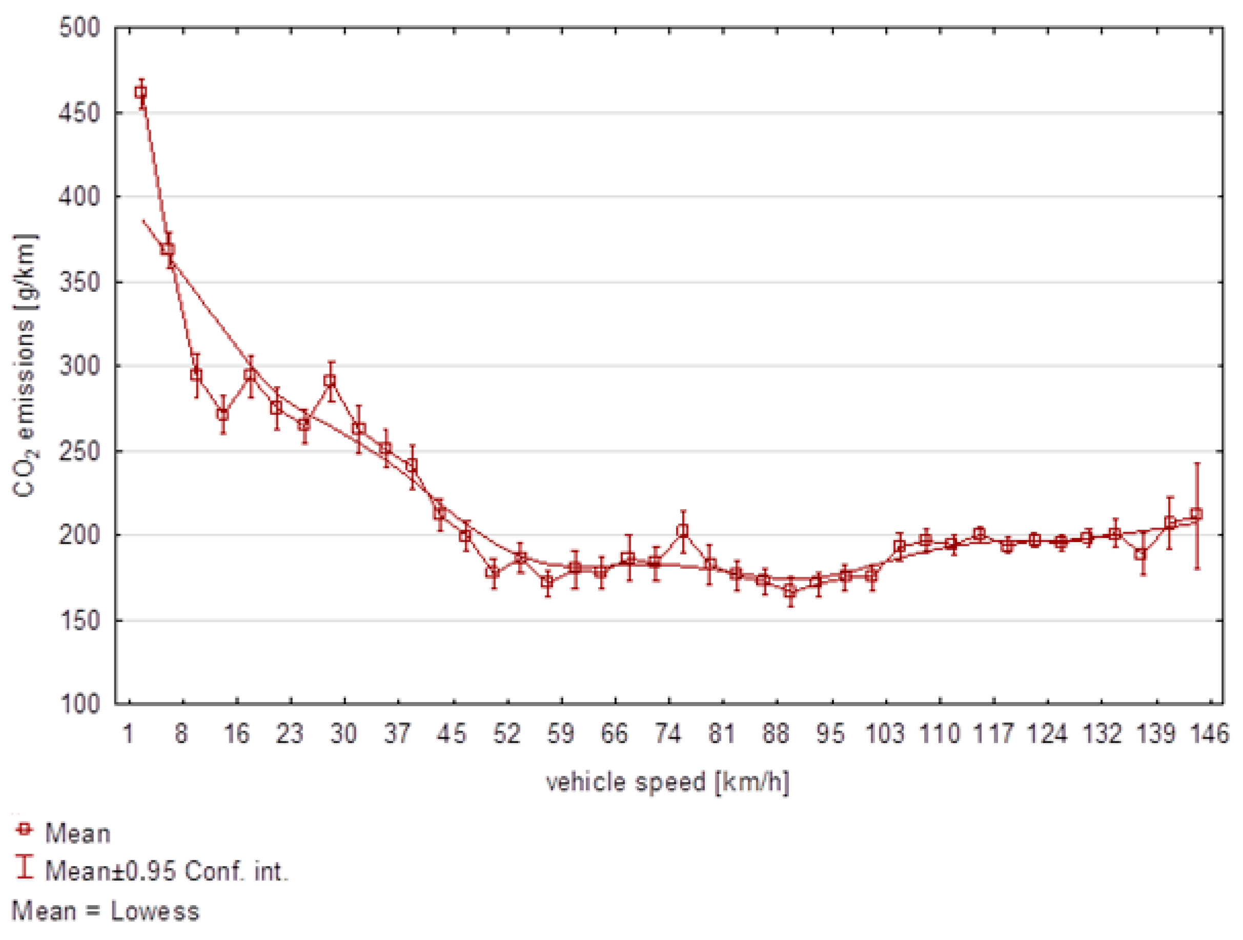
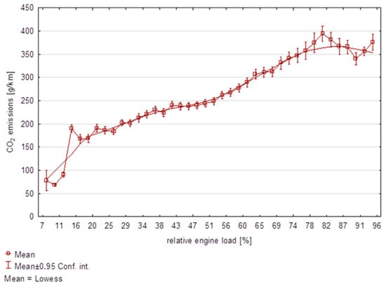
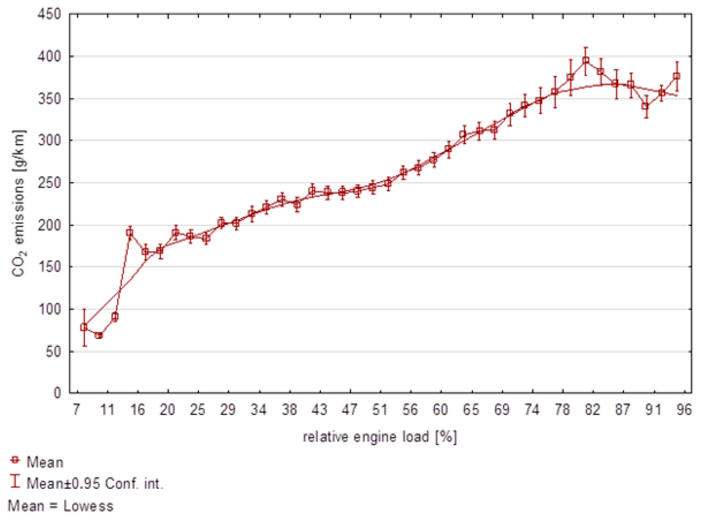
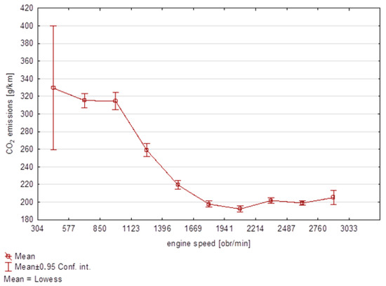
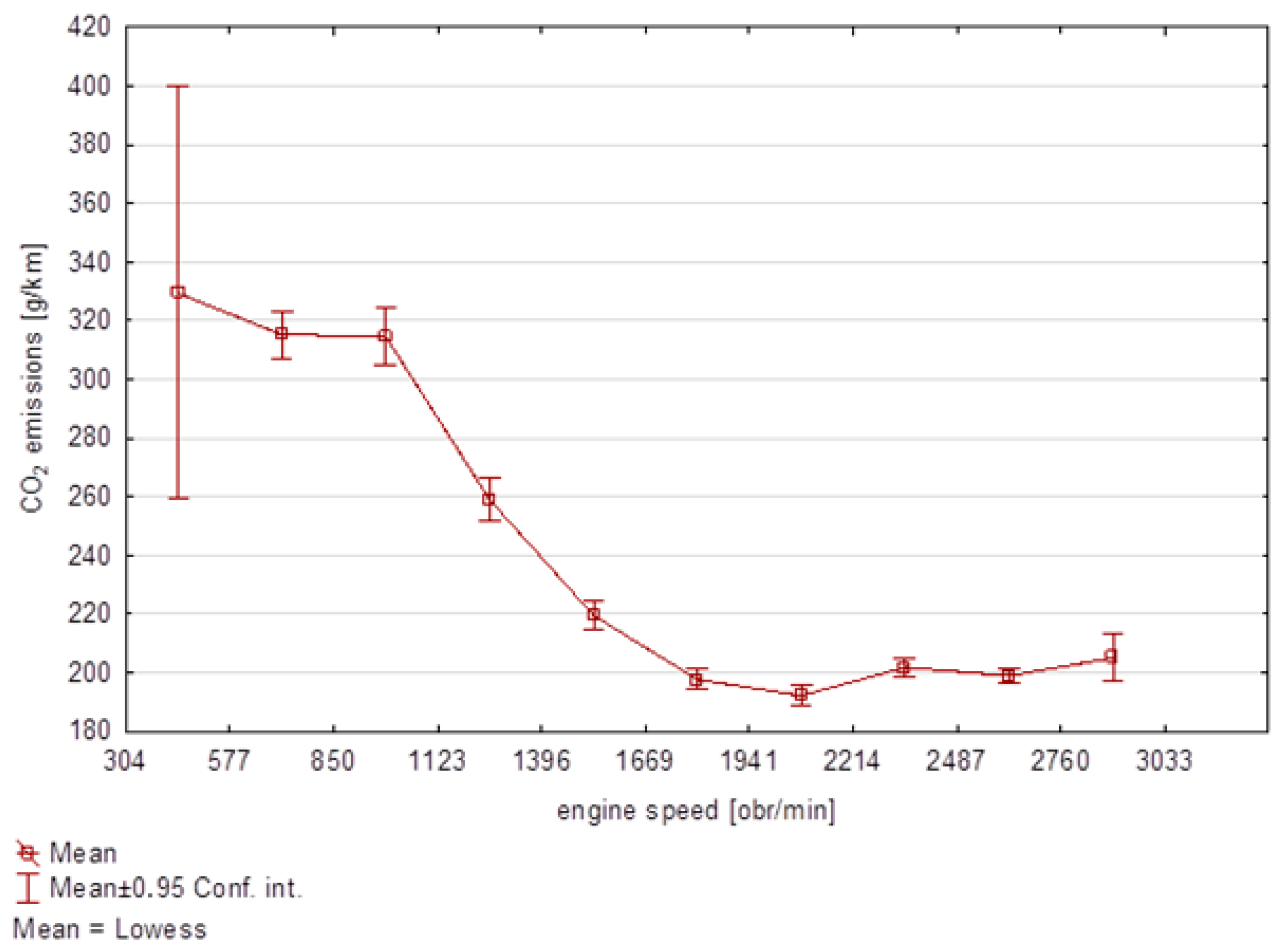
In the next step, the linearity of the selected dependent variables in relation to the CO₂ variable was checked (Figure 5, Figure 6, Figure 7 and Figure 8). The speed of the vehicle was analyzed first.

Figure 5. CO₂ emissions depending on vehicle speed.

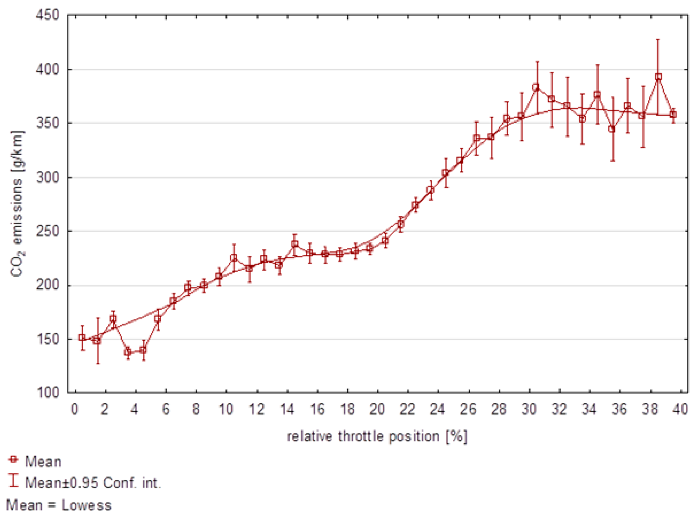
Figure 6. CO₂ emission as a function of relative throttle position.

Figure 7. CO₂ emission as a function of relative engine load.

Figure 8. CO₂ emission as a function of engine speed.

The above analysis showed that the level of CO₂ emissions varies significantly depending on the vehicle speed. The average CO₂ emission at low speeds is higher than at higher speeds. Subsequently, plots of the variables relative throttle position, relative engine load, and engine speed (RPM) were generated (Figure 6, Figure 7 and Figure 8).

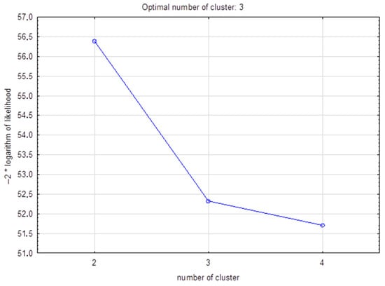
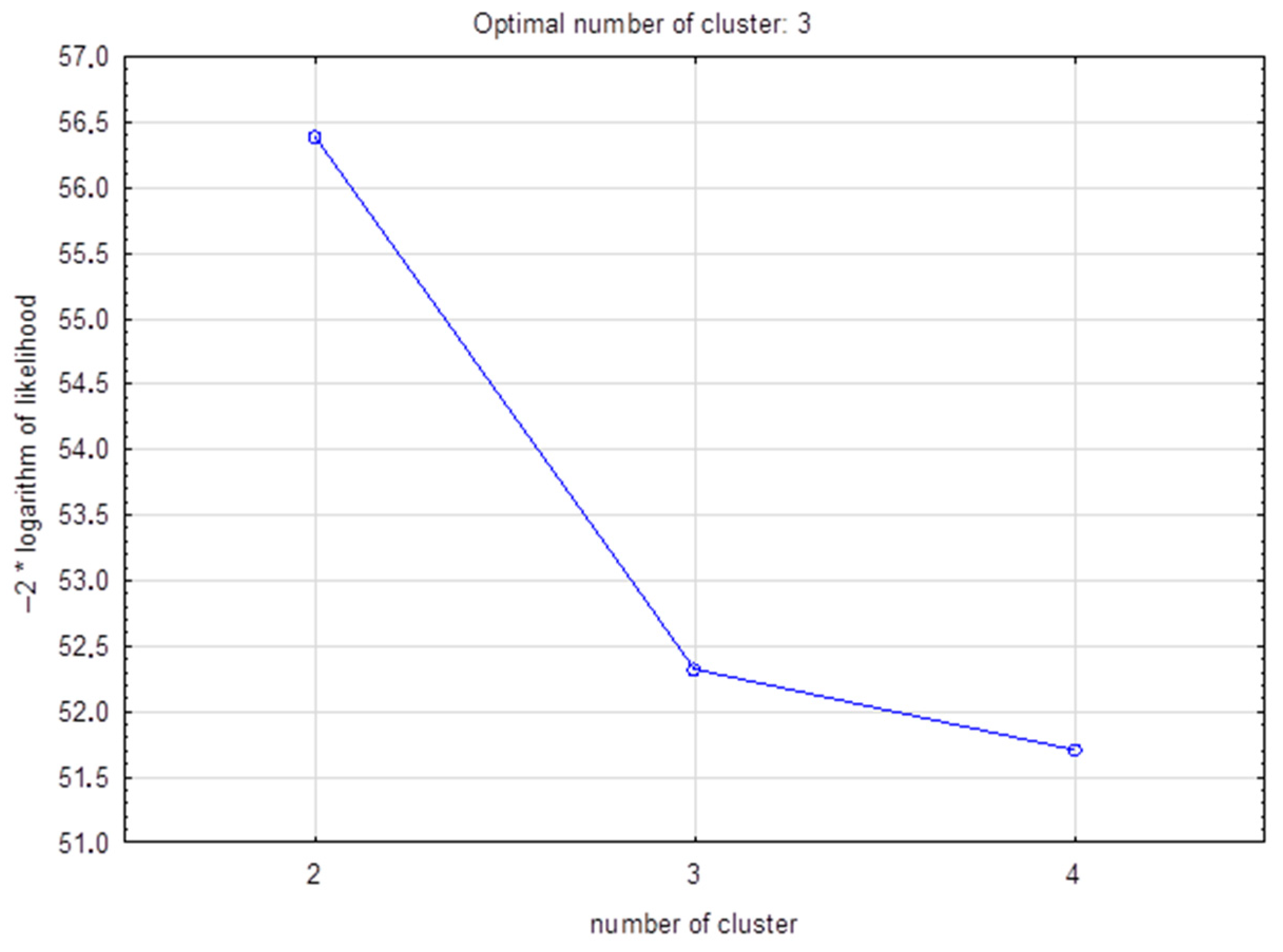
Due to the high variability observed, the subsequent analysis involved dividing the observations into similar groups. For this purpose, the k-means clustering method was applied. In the first step, using the elbow method, the optimal number of clusters was determined (Figure 9), and then, three homogeneous groups of observations were identified within the analyzed dataset.

Figure 9. Optimal number of clusters determined using the elbow method.

The mean values of individual variables within the identified groups are presented in Table 3, while their frequencies are shown in Table 4.

Table 3. Means of variables in individual clusters.

Cluster No.	Linear Speed of the Vehicle [v] [km/h]	Relative Engine Load L% [%]	Engine Speed in RPM n [obr/min]	Engine Power P [kW]	Engine Torque T [Nm]	Throttle Position φ% [%]	CO2 Emissions ${\mathit{m}}_{{\mathit{C}\mathit{O}}_{\mathbf{2}}}$ $[\mathbf{g}/\mathbf{k}\mathbf{m}]$
1	16.78	24.65	1411.49	4.41	28.70	6.95	365.60
2	105.68	42.48	2252.47	9.85	41.82	15.93	166.25
3	49.17	66.64	1910.11	14.36	67.70	26.03	213.40

Table 4. Number of observations in clusters.

Number of Cluster	Number of Observations	Share (%)
1	3846	16.86
2	9318	40.85
3	9647	42.29

The above analysis of the emission function in relation to the selected parameters demonstrated that the available database should be divided into three groups, corresponding to the engine operating modes, namely: the vehicle start-up mode (cluster 1), the urban driving mode (cluster 3), and the extra-urban driving mode (cluster 2). The average vehicle speeds for these modes were 16 km/h, 49 km/h, and 105 km/h, respectively. It can be assumed that the vehicle start-up mode includes speeds of up to approximately 35 km/h, the urban driving mode covers speeds up to 85 km/h, while the extra-urban driving mode refers to speeds above 85 km/h.

To confirm the validity of the proposed division, a homogeneity test was performed for the selected subgroups. The selection of the test was preceded by an analysis of the distribution patterns of the CO₂ emission variable in each group. As the first step, the assumption of normal distribution was verified by applying the Kolmogorov–Smirnov test, in which the test statistic D was calculated. The results are presented in Table 5.

Table 5. Results of the Kolmogorov–Smirnov test for the normality of the CO₂ emission variable.

Driving Mode	Value of Test Statistic	p Value
Vehicle start-up	0.13	0.01
Urban	0.04	0.01
Extra-urban	0.12	0.00

Due to the failure to meet the assumptions required for conducting ANOVA, the Kruskal–Wallis test was used to compare the variable across the three groups. The calculated value of the test statistic T and the corresponding p-value are presented in Table 6.

Table 6. Kruskal–Wallis test results.

Kruskal–Wallis: T = 5631.46 p = 0.00
Driving Mode	Total of Ranks	Average Rank
Vehicle start-up	71,268,902	18,516.21
Urban	103,018,512	10,673.28
Extra-urban	85,894,852	9226.09

The calculated p-value is smaller than the adopted significance level α = 0.05; therefore, the null hypothesis should be rejected, and the alternative hypothesis stating that there are differences in the mean values among the groups should be accepted.

Subsequently, a Tukey post hoc test with the Kramer correction was conducted to examine the significance of differences in mean CO₂ emission values among the clusters. The calculated test statistics q and their corresponding p-values (Table 7) did not allow the acceptance of the null hypothesis that the compared group means do not differ statistically.

Table 7. Results of the Tukey–Kramer test.

Driving Mode	Vehicle Start-Up 365.60 g/km	Urban 213.40 g/km	Extra-Urban 166.25 g/km
Vehicle start-up		0.00	0.00
Urban			0.00
Extra-urban	0.00	0.00

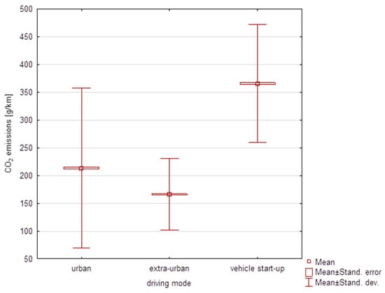
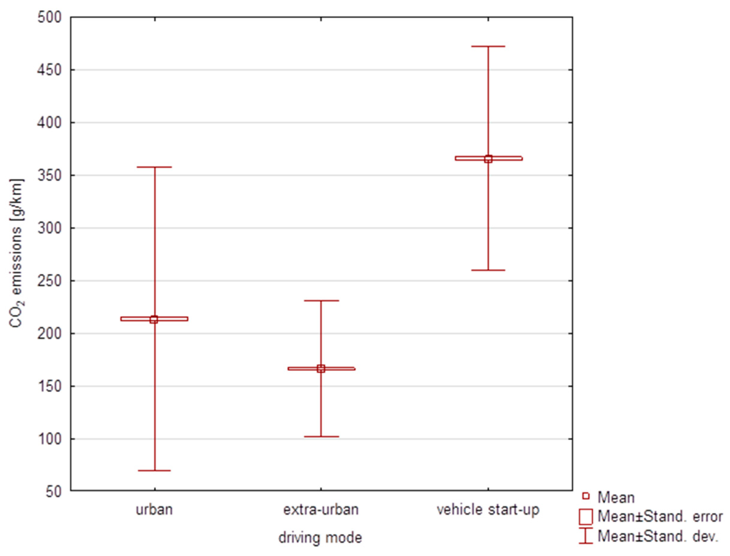
The identified differences are shown in Figure 10, which presents a box plot of CO₂ emissions depending on the driving mode.

Figure 10. Average CO₂ emissions depending on driving mode.

3.1. Multiple Regression Model of CO₂ Emissions During Vehicle Start-Up

In the next stage of the study, a multiple regression model was developed to assess CO₂ emissions at the moment of vehicle start-up. The independent variables included vehicle linear speed, relative engine load, engine rotational speed, engine power, torque, and relative throttle position.

In the first step, the data were analyzed using selected descriptive statistics recorded during the initial phase of vehicle movement (Table 8). The mean, median, and standard deviation values were examined.

Table 8. Basic descriptive statistics of variables in the vehicle start-up cluster.

Variable Studied	Mean	Median	Standard Deviation
maximum speed $v$ [km/h]	16.78	17.00	1.00
relative engine load $L_{\%}$ [%]	28.65	25.10	7.06
rotational engine speed $n$ [rpm]	1130.42	1121.50	304.25
engine power $P$ [kW]	4.06	2.82	0.07
torque $T$ [Nm]	32.15	24.69	0.46
relative throttle position ${\phi }_{\%}$ [%]	7.53	5.49	0.39
CO2 emission $m_{{CO}_2}$ [g/km]	365.85	360.01	105.82

The average vehicle linear speed during start-up is 16 km/h, with an average CO₂ emission value of 365 g/km. The calculated standard deviations for CO₂ emissions and engine rotational speed indicate high variability in these data. Next, a correlation analysis of all examined variables was conducted. For this purpose, the Pearson correlation coefficient was used (Table 9).

Table 9. Correlation coefficients of independent and dependent variables in vehicle start-up mode.

Variable Studied	Vehicle Speed v [km/h]	Relative Engine Load L% [%]	Rotational Engine Speed n [rpm]	Engine Power P [kW]	Torque T [Nm]	Relative Throttle Position [%] φ%	CO2 Emissions ${\mathit{m}}_{{\mathit{C}\mathit{O}}_2}$ [g/km]
vehicle speed $v$ [km/h]	1.00	0.10	0.84	0.50	0.34	0.27	−0.37
relative engine load $L_{\%}$ [%]		1.00	0.15	0.84	0.47	0.43	0.61
rotational engine speed $n$ [rpm]			1.00	0.72	0.33	0.29	−0.16
engine power $P$ [kW]				1.00	0.94	0.45	0.03
torque $T$ [Nm]					1.00	0.45	0.07
relative throttle position ${\phi }_{\%}$ [%]						1.00	0.51

The analysis showed that the correlation coefficient between vehicle speed and engine rotational speed is 0.84. A similarly high value was calculated for relative engine load and engine power (0.84). High correlation coefficients were also observed for engine power and torque (0.94) and engine rotational speed (0.72). These high correlation values indicate significant multicollinearity among the analyzed variables, reflecting informational redundancy (a violation of one of the regression model assumptions). Therefore, engine rotational speed, torque, and engine power were excluded from further analysis. Before constructing the model, the dataset was divided into two samples, representing 90% and 10% of the entire set, which were then used as the training and test sets, respectively. This division allows for the assessment of whether the model achieves satisfactory prediction results for data not used in model construction and enables verification of its generalization ability, confirming its practical applicability.

In the first step, the model parameters were estimated and then tested for statistical significance. A Student’s t-test was performed, calculating the test statistic t and the corresponding p-value. For all variables, p = 0.00, indicating no grounds to accept the null hypothesis. The estimated parameter values are therefore significantly different from zero. The estimated parameter values, along with the test statistics and corresponding p-values, are presented in Table 10.

Table 10. Estimated parameter values of the multiple regression model in vehicle start-up mode.

N = 3475	Summary of the Regression of the Dependent Variable: CO2 Emissions R2 = 0.70, F(33,471) = 1164.4, p < 0.00 Estimation Standard Error: 74.74 g/km
	b	t(3471)	p Value
Absolute term	358.72	71.55	0.00
Vehicle speed	−2.59	−57.94	0.00
Relative engine load	3.06	19.40	0.00
Relative throttle position	−0.75	−2.48	0.01

Next, the model was evaluated. First, the coefficient of determination R2 was calculated, which equals 70%. This indicates that the model explains 70% of the variability in the CO₂ emission variable, which can be considered a good result.

The overall significance of the structural parameters was also tested. The calculated value of the test statistic in the generalized Wald test is $F=1164.4$, with a corresponding p-value = 0.00, indicating that all regression coefficients in the model are significantly different from zero. Based on this, the regression model equation was obtained:

$$y=358.71- 2.59·V+3.06·L_{\%}-0.75·{\phi }_{\%},$$

where V—vehicle speed, $L_{\%}$—relative engine load, ${\phi }_{\%}$—throttle position.

Next, the residuals’ distribution was examined, beginning with an assessment of conformity to the normal distribution. The calculated Chi-square test statistic is 267.18, with a corresponding p-value = 0.09, indicating no grounds to reject the null hypothesis that the residuals follow a normal distribution.

To verify the assumption of no residual autocorrelation, the autocorrelation function (ACF) and the partial autocorrelation function (PACF) of the random component were determined. No statistically significant autocorrelation values were observed, indicating that the residuals of the model are randomly distributed. Additionally, the Durbin–Watson test was performed. The calculated test statistic for the Durbin–Watson test is $DW=1.925$, while the lower and upper critical values are $dL=1.91$ and $dU=1.92$, respectively. Since the test statistic is less than 2 and greater than the upper critical value, it can be concluded that there is no autocorrelation in the residual component.

Next, the heteroscedasticity of the residuals was examined using White’s test. The calculated test statistic is $F=38.81$, with a corresponding p-value = 0.08. This indicates no grounds to reject the null hypothesis, allowing the assumption that the variance of the residual component does not vary across explanatory variables, i.e., the homoscedasticity assumption is satisfied (residual variance is uniform).

The above analyses confirm the correctness of the model, and therefore, in the next stage, a goodness-of-fit assessment was performed. For this purpose, a test data set was used, separated from the same sample as the training data set. This made it possible to verify whether the model has appropriate and satisfactory predictive properties. Key fit metrics were calculated and are presented in Table 11.

Table 11. Estimated prediction errors and information criterion in vehicle start-up mode.

Metric Name	Metric Value
Mean squares residuals (MSE)	4452.71
Mean absolute error	37.79
Relative mean squared error	27.60
Relative average deviation (MRAE)	0.48
Mean absolute prediction error (MAPE)	0.20
AIC criterion	39,373.26

The mean absolute error (MAE) of the model is 27.60 g/km, indicating the average distance between predicted and observed values. For the average CO₂ emission in this cluster, which is 365.85 g/km, this result can be considered good. The mean absolute percentage error (MAPE) is approximately 20%, reflecting the average magnitude of the prediction error, which is a satisfactory result. These metrics indicate that the model’s predictive capabilities are at a good level.

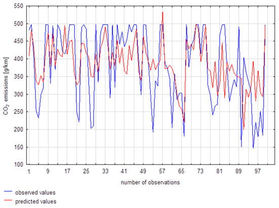
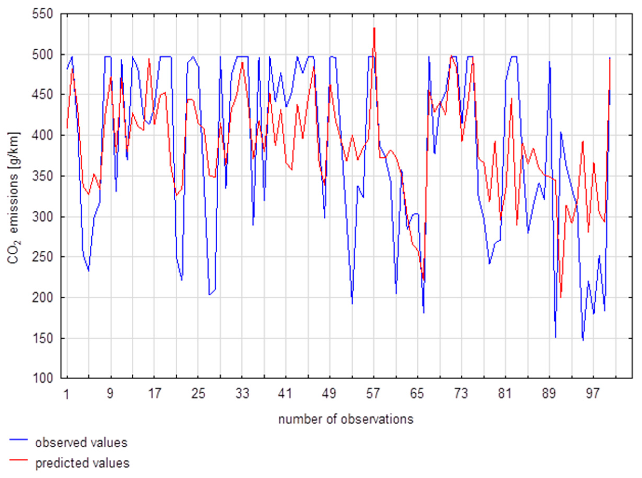
Next, a plot of observed versus predicted values was generated (Figure 11).

Figure 11. Observed and predicted values for the multiple regression model in vehicle start-up mode.

Visual inspection shows that the model closely follows the empirical data, appropriately responding to increases and decreases in the predicted values.

3.2. Multiple Regression Model of CO₂ Emissions in Urban Driving Mode

Next, a model for CO₂ emissions during urban driving was developed. In the first step, the data were analyzed using selected descriptive statistics, calculating the mean, median, and standard deviation values (Table 12).

Table 12. Basic descriptive statistics of variables in urban driving mode.

Variable Studied	Mean	Median	Standard Deviation
vehicle speed [km/h]	49.17	49.00	10.64
relative engine load [%]	32.37	28.63	18.72
rotational engine speed [rpm]	1738.33	1735.75	247.57
engine power [kW]	8.23	6.11	5.23
torque [Nm]	44.65	32.50	26.50
relative throttle position [%]	11.70	8.63	10.14
CO2 emissions [g/km]	213.21	175.52	144.24

The average vehicle linear speed in this cluster is 49 km/h, which is close to the median, indicating the absence of extreme outliers in its distribution and a roughly symmetrical distribution. The average CO₂ emission is 213 g/km, with a median of 175 g/km and a standard deviation of 144.24 g/km. This indicates high variability in this variable. Next, the relationships between the independent variables and the dependent variable were analyzed. For this purpose, the Pearson correlation coefficient was used. The results are presented in Table 13.

Table 13. Correlation coefficients of independent and dependent variables.

Variable Studied	Linear Vehicle Speed [km/h]	Relative Engine Load [%]	Rotational Engine Speed [rpm]	Engine Power [kW]	Torque [Nm]	Relative Throttle Position [%]	CO2 Emissions [g/km]
linear vehicle speed [km/h]	1.00	0.06	0.25	0.12	0.07	0.12	−0.20
relative engine load [%]		1.00	−0.01	0.83	0.58	0.24	0.82
rotational engine speed [rpm]			1.00	0.75	0.07	0.05	0.08
engine power [kW]				1.00	0.97	0.49	0.47
torque [Nm]					1.00	0.52	0.49
relative throttle position [%]						1.00	0.69

The correlation coefficient was calculated to be high for engine power and torque (0.97), relative engine load (0.83), and engine rotational speed (0.75). Therefore, engine torque, engine rotational speed, and engine power were excluded from further analysis. It should also be noted that all selected variables exhibit a linear relationship with the dependent variable.

Next, the model was constructed. Once again, the training data set was used as a basis. In the first step, the model parameters were estimated and then tested for statistical significance. A Student’s t-test was applied, calculating the test statistic t and the corresponding p-value. The estimated parameter values, along with the test statistics and p-values, are presented in Table 14. For all variables, p = 0.00, indicating no grounds to accept the null hypothesis, and therefore the estimated parameters are significantly different from zero.

Table 14. Estimated parameters of the multiple regression model in urban driving mode.

N = 8712	Summary of the Regression of the Dependent Variable: CO2 Emissions R2 = 0.63; F(3.8708) = 4894.9 p < 0.00 Estimation Standard Error: 88.02
	b	t(8708)	p Value
Absolute term	182.84	62.74	0.00
Linear speed of the vehicle	−4.11	−78.18	0.00
Relative engine load	4.23	32.40	0.00
Relative throttle position	9.02	25.69	0.00

Based on this, a formal verification of the model was conducted. The coefficient of determination (R²) of the model is 63%, indicating that 63% of the variability between the variables is explained by the model, which can be considered satisfactory.

The overall significance of the structural parameters was also tested. The calculated value of the test statistic in the generalized Wald test is $F=4894.9$, with a corresponding p-value = 0.00, indicating that the null hypothesis should be rejected in favor of the alternative.

Thus, all estimated parameters in the model are significantly different from zero. Based on this, the regression model equation was obtained:

$$y=182.84- 4.11·V+4.23·L_{\%}+9.02·{\phi }_{\%},$$

where $V$—linear vehicle speed, $L_{\%}$—relative engine load, ${\phi }_{\%}$—throttle position.

Next, the residuals’ distribution was examined, beginning with a check for conformity to the normal distribution. The calculated Chi-square test statistic is 1761.49, with a corresponding p-value = 0.07, indicating no grounds to reject the null hypothesis; therefore, the residuals follow a normal distribution.

Subsequently, residual autocorrelation was assessed using the Durbin–Watson test. The autocorrelation function and partial autocorrelation function of the random component were determined. No statistically significant autocorrelation values were observed, indicating that the residuals are randomly distributed.

Next, the value of the DW test statistic was calculated and the critical values $dL$ and $dU$ were determined, assuming $k=6$ (number of model parameters) and $T=8712$ (number of observations). The calculated value of the test statistic is $DW=1.94$, while the threshold values are $dL=1.92$ and $dU=1.93$. The test statistic is less than 2 and greater than the upper critical value, which allows the conclusion that there is no autocorrelation in the residual component (there are no grounds to reject the null hypothesis).

Next, the assumption of heteroscedasticity of the residuals was tested. The calculated test statistic in White’s test is $F=111.28$, with a corresponding p-value = 0.06, indicating no grounds to reject the null hypothesis.

This suggests that the random component is homoscedastic, meaning its variance remains constant across different values of the explanatory variables.

This analysis confirmed that the assumptions of the regression model are satisfied, validating the model. Consequently, the test dataset was used to assess the model’s goodness of fit, and the key error metrics of the model were estimated (Table 15).

Table 15. Estimated prediction errors and information criterion in urban driving mode.

Metric Name	Metric Value
Mean squares residuals (MSE)	7513.39
Mean absolute error	60.57
Relative mean squared error	3.45
Relative average deviation (MRAE)	0.52
Mean absolute prediction error (MAPE)	0.38
AIC criterion	10,261.56

The mean absolute error of the model is 60.57 g/km, indicating the average deviation between the predicted and observed values. For the mean CO₂ emission value in this cluster, amounting to 213.21 g/km, this result can be considered satisfactory. The mean absolute percentage error is 38%, which reflects the average magnitude of the prediction error and can be regarded as an acceptable level. The above results indicate that the predictive capabilities of the model are at a satisfactory level.

Next, a plot of observed versus predicted values was generated (Figure 12).

Figure 12. Observed and predicted values for the model in urban driving mode.

The model follows the data, accurately reflecting the nature of CO₂ emissions variability.

3.3. Multiple Regression Model of CO₂ Emissions in Extra-Urban Driving Mode

As the next step, a model of CO₂ emissions to the environment during extra-urban driving was developed using a multiple regression approach. The analysis began with the calculation of selected descriptive statistics, including the median, mean, and standard deviation (Table 16).

Table 16. Basic Descriptive Statistics of the Model in Extra-Urban Driving Mode.

Variable Studied	Mean	Median	Standard Deviation
vehicle speed [km/h]	105.68	108.00	17.92
relative engine load [%]	48.55	47.84	20.24
rotational engine speed [rpm]	2263.58	2290.00	311.19
engine power [kW]	11.02	9.56	4.60
torque [Nm]	46.82	37.60	19.85
relative throttle position [%]	20.36	18.43	14.21
CO2 emissions [g/km]	166.25	172.53	64.60

The average linear velocity of the vehicle in extra-urban driving mode is 105 km/h, with an average CO₂ emission level of 166 g/km. The mean CO₂ emission value is lower than the median, which indicates that the distribution of this variable is left-skewed. A high standard deviation value was also observed, indicating substantial variability in the data. Subsequently, the Pearson correlation coefficient was calculated for the explanatory variables and the dependent variable (Table 17).

Table 17. Correlation Coefficients of Explanatory and Dependent Variables in Extra-Urban Driving Mode.

	Vehicle Speed [km/h]	Relative Engine Load [%]	Rotational Engine Speed [rpm]	Engine Power [kW]	Torque [Nm]	Relative Throttle Position [%]	CO2 Emissions [g/km]
vehicle speed [km/h]	1.00	0.22	0.89	0.13	−0.15	0.05	0.14
relative engine load [%]		1.00	0.20	0.82	0.94	0.38	0.91
rotational engine speed [rpm]			1.00	0.77	−0.14	0.05	0.18
engine power [kW]				1.00	0.94	0.48	0.38
torque [Nm]					1.00	0.49	0.33
relative throttle position [%]						1.00	0.69

The conducted analysis showed that the correlation coefficient between vehicle speed and engine speed is 0.89. Similarly high values were obtained for the variables relative engine load and torque (0.94), as well as engine power (0.82). The high correlation coefficients among the analyzed variables indicate significant multicollinearity, implying informational redundancy and a violation of one of the assumptions of the regression model. Due to this violation (high correlation values between variables), the variables engine speed, torque, and engine power were excluded from further analysis.

Subsequently, parameter estimation for the model was carried out according to the adopted procedure, and the parameters were tested for statistical significance. The t-Student test was applied, and the t statistic as well as the corresponding p-value were calculated.

The estimated parameter values, along with the t-statistic and the obtained p-value, are presented in Table 18. For all variables, the p-value equals 0.00, which means there are no grounds for accepting the null hypothesis; therefore, the estimated parameters are statistically significantly different from zero.

Table 18. Estimated parameters of the multiple regression model in extra-urban driving mode.

N = 8380	Summary of the Regression of the Dependent Variable: CO2 Emissions R2 = 0.78; F(3.8376) = 9910.2, p < 0.00 Estimation Standard Error: 30.19
	b	t(8376)	p Value
Absolute term	56.51	34.70	0.00
Vehicle speed	−0.56	−33.54	0.00
Relative engine load	3.21	63.93	0.00
Relative throttle position	1.92	14.92	0.00

Subsequently, the formal verification of the model was carried out. The coefficient of determination R² equals 0.78, which indicates that 78% of the relationships between the variables are explained by the model.

The joint significance of the structural parameters was also tested using the Fisher–Snedecor test. The calculated value of the test statistic (46) is $F=9910.2$ and the corresponding probability level is $p=0.00$, which means that the null hypothesis should be rejected in favor of the alternative hypothesis, and therefore all of the estimated parameters differ significantly from zero. Based on this, the regression model equation was obtained:

$$y=56.51- 0.56· V+3.21· L_{\%}+1.92·{\phi }_{\%}$$

where $V$—vehicle speed, $L_{\%}$—relative engine load, ${\phi }_{\%}$—throttle position.

Subsequently, an analysis of the residual distribution was conducted, beginning with an assessment of its conformity to the normal distribution. The calculated value of the chi-square test statistic is 7.28, and the corresponding probability level p = 0.20 indicates that there are no grounds for rejecting the null hypothesis. Therefore, the residuals follow a normal distribution.

In the next step, the autocorrelation and partial autocorrelation functions of the random component were determined. No statistically significant autocorrelation values were found, which means that the residual distribution of the model is random. Additionally, the Durbin–Watson test was performed. The calculated value of the test statistic is $DW=1.81$, while the threshold values are $dL=1.79$ and $dU=1.80$. The calculated value of the test statistic is greater than 2 and above the upper critical value, which indicates the absence of autocorrelation in the residual component.

Next, White’s test was conducted to examine the presence of heteroscedasticity in the residuals. The calculated test statistic is $F=39.92$, with a corresponding p-value = 0.07, indicating no grounds to reject the null hypothesis.

This suggests that the random component is homoscedastic, meaning its variance does not vary across the values of the explanatory variables.

These results confirm that the model is valid. After positive verification, the goodness of fit was assessed. In the first step, prediction errors and the AIC (Akaike Information Criterion) were estimated (Table 19).

Table 19. Estimated prediction errors and information criterion in extra-urban driving mode.

Metric Name	Metric Value
Mean squares residuals (MSE)	1145.47
Mean absolute error	19.62
Relative mean squared error	0.27
Relative average deviation (MRAE)	0.18
Mean absolute prediction error (MAPE)	0.19
AIC criterion	79,686.44

The mean absolute error (MAE) of the model is 19.62 g/km, indicating the average deviation between the predicted and observed values. For the mean CO₂ emission in this cluster, which is 166.25 g/km, this result can be considered very good. The mean absolute percentage error (MAPE) is approximately 19%, reflecting the average magnitude of the prediction error, which is a satisfactory result. These metrics indicate that the model’s predictive capabilities are at a good level.

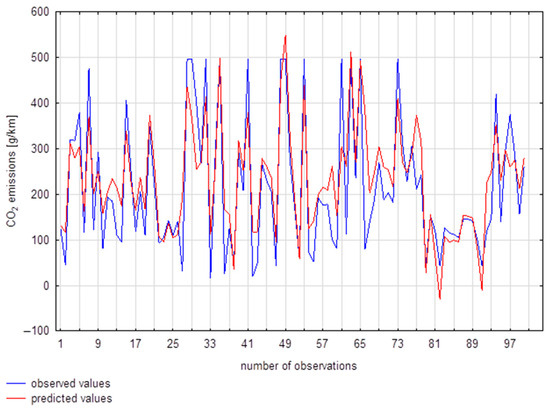
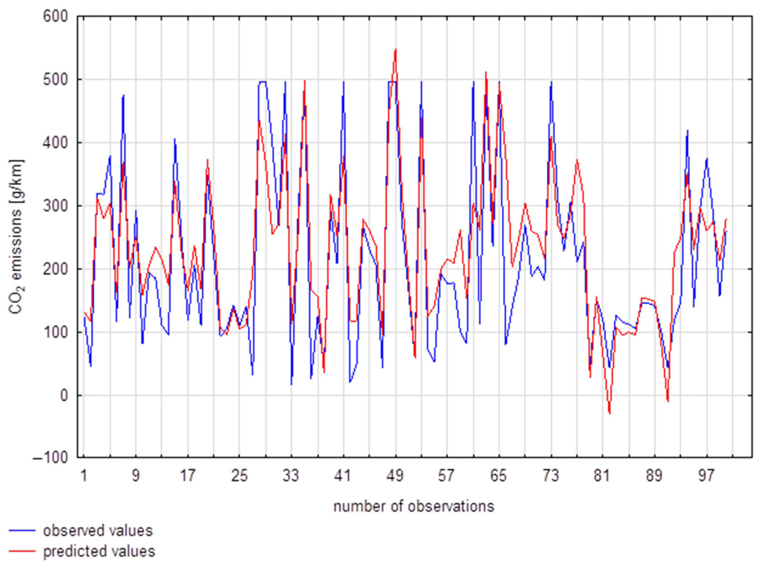
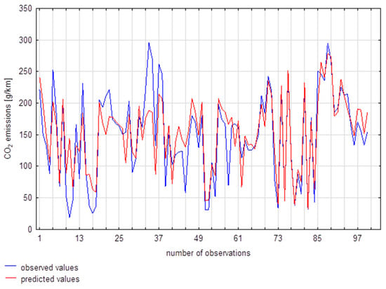
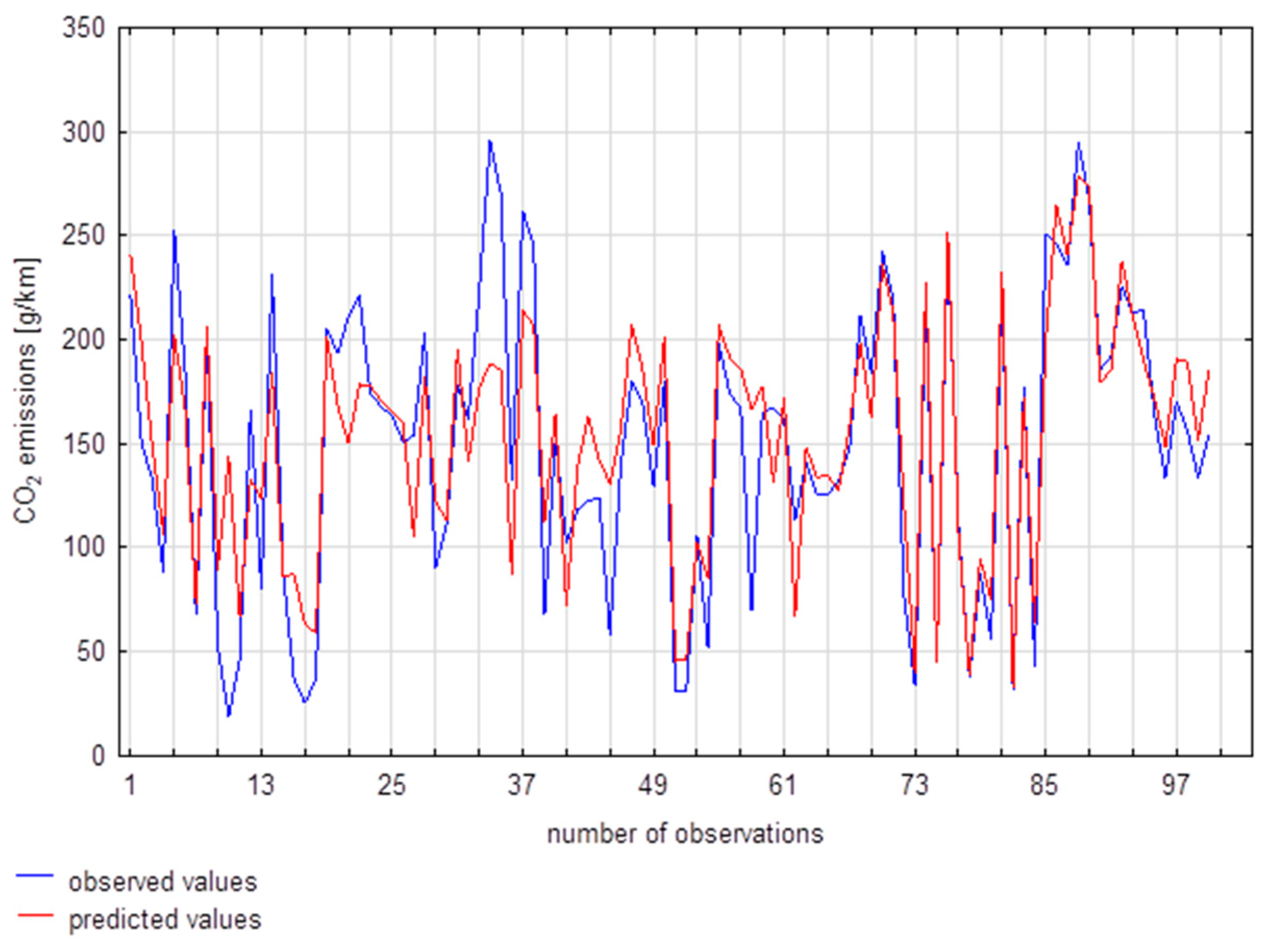
Next, a plot of the observed and predicted values was generated (Figure 13).

Figure 13. Observed and predicted values for the multiple regression model in extra-urban driving mode.

Visual inspection shows that the constructed model closely follows the data, accurately reflecting both decreases and increases in the modeled values.

4. Discussion

In addition to the classical linear regression approaches discussed in the presented article, more advanced time-series modeling techniques have been used for emission prediction. Autoregression with exogenous variables (VARX) models have been applied to capture temporal dependencies in vehicle emission data [28]. Other approaches involved the use of deep learning (MLP with 5 hidden layers) for CO₂ emission prediction, achieving high accuracy (R² = 0.9938) [29]. The application of portable emissions measurement systems (PEMS) combined with OBD data and artificial neural networks can form the basis of the real driving emission (RDE) prediction [30]. However, this approach is impractical due to the use of the high-cost PEMS.

Table 20 presents a summary of the estimated intercepts and coefficients of the parameters for the three models. It should be noted that the highest average CO₂ emission occurs during vehicle start-up (365.60 g/km), while the lowest occurs during extra-urban driving (166.18 g/km).

Table 20. Comparison of multiple regression model parameters across the three driving modes.

Explanatory Variable	Parameter Value in Vehicle Start Mode	Parameter Value in Urban Driving Mode	Parameter Value in Extra-Urban Driving Mode
Absolute term	358.72	182.84	56.51
Vehicle speed	−2.59	−4.11	−0.56
Relative engine load	3.06	4.23	3.21
Relative throttle position	−0.75	9.02	1.92

Regardless of the driving mode (vehicle start-up, urban driving, extra-urban driving), any increase in vehicle speed leads to a reduction in CO₂ emissions to the environment. During vehicle start-up, each 1 km/h increase in speed reduces CO₂ emissions by 2.59 g/km; during urban driving, emissions decrease by 4.11 g/km; and during extra-urban driving, they decrease by 0.56 g/km.

For the variable relative engine load, each 1% increase results in a CO₂ emission increase of 3.06 g/km, 4.23 g/km, and 3.21 g/km for vehicle start-up, urban driving, and extra-urban driving, respectively.

For the variable relative throttle position, a 1% increase during vehicle start-up leads to a decrease in CO₂ emissions by 0.75 g/km. During urban and extra-urban driving, a 1% increase in this variable causes CO₂ emissions to increase by 9.02 g/km and 1.92 g/km, respectively.

Analysis of the individual models (Table 21) showed that the highest estimation error occurs in the urban driving regression model (88.02 g/km), while the lowest error is observed in the extra-urban driving model (30.19 g/km). This is because the average CO₂ emissions are highest when the vehicle is moving at low speeds. The lowest mean absolute error is found in the extra-urban driving model (19.62 g/km), while the highest is in the urban driving model (60.57 g/km).

Table 21. Comparison of the goodness of fit of the multiple regression models.

Model	Estimation Error	Mean Absolute Error (MSE)	Relative Mean Squared Error	Relative Average Deviation (MRAE)	Mean Absolute Prediction Error (MAPE)
Vehicle start mode	74.74	37.79	27.60	0.48	0.20
Urban driving mode	88.02	60.57	3.45	0.52	0.38
Extra-urban driving mode	30.19	19.62	0.27	0.18	0.19

The developed models also allowed for detailed conclusions. In the case of multivariate regression models, it was found that:

Regardless of the driving mode, an increase in vehicle speed by 1 km/h results in a decrease in CO₂ emissions.

A 1% increase in relative engine load leads to an increase in CO₂ emissions. The largest effect was observed in urban driving (4.23 g/km).

A 1% increase in relative throttle position leads to a decrease in CO₂ emissions by 0.75 g/km during vehicle start-up, while in other modes it causes an increase (urban: 9.02 g/km, extra-urban: 2.34 g/km).

The studies confirmed that the highest average CO₂ emissions occur during vehicle start-up (365.60 g/km), while the lowest occur during extra-urban driving (166.18 g/km). Regardless of the driving mode, an increase in vehicle speed leads to a reduction in CO₂ emissions to the environment. During vehicle start-up, each 1 km/h increase in speed reduces CO₂ emissions by 2.59 g/km; during urban driving, emissions decrease by 4.11 g/km; and during extra-urban driving, they decrease by 0.56 g/km. A 1% increase in relative engine load results in a CO₂ emission increase of 3.06 g/km, 4.23 g/km, and 3.21 g/km for vehicle start-up, urban driving, and extra-urban driving, respectively. A 1% change in relative throttle position causes CO₂ emissions to decrease by 0.75 g/km during vehicle start-up and to increase by 9.02 g/km and 2.34 g/km during urban and extra-urban driving, respectively. Furthermore, analysis of the individual models showed that the urban driving regression model has the highest estimation error (88.02 g/km), while the extra-urban driving model has the lowest (30.19 g/km). Regarding mean absolute errors, the vehicle start-up model exhibits the lowest value (37.79 g/km), whereas the urban driving model has the highest (60.57 g/km).

The developed models are applicable to gasoline-powered internal combustion engines. The models cannot be directly applied to hybrid electric vehicles (HEV), plug-in hybrid electric vehicles (PHEV), battery electric vehicles (BEV), or diesel engines.

5. Conclusions

The application of multiple regression methods for modeling CO₂ emissions allowed not only for understanding the general relationships that describe CO₂ emissions but also for identifying specific factors whose control can contribute to their reduction. The article demonstrated that monitoring vehicle speed, relative engine load, and relative throttle position during driving enables such control. Consequently, an individual passenger vehicle driver, regardless of the driving mode, can influence CO₂ emissions. This shows that the measurable and user-controllable factors listed above have a significant impact on CO₂ emission levels, which constituted the first specific objective of this study. It is also worth emphasizing that, unlike standard laboratory tests—which often rely on averaged parameters and assumed driving conditions—OBD data analysis allows for accounting for dynamic changes arising from real vehicle usage, such as variations in speed, engine load, engine rotational speed, torque, engine power, and relative throttle position.

It is recommended to maintain relative engine load at no more than 45–50% and avoid opening the throttle above 50%. When driving, it is advisable to drive at a steady, moderate speed, limiting frequent speed changes and sudden acceleration and braking. In urban driving conditions, it is recommended to drive at the highest possible speed limit in the area, while when driving outside urban areas, maintain a constant speed between 85 and 140 km/h, as CO₂ emissions and fuel consumption increase dramatically above 140 km/h.

Moreover, the study found that the OBD interface, commonly used in passenger vehicles, can serve as an excellent tool for mitigating negative environmental impacts, accessible to individual users without additional costs. Continuous access to selected engine operating parameters and other key vehicle performance characteristics allows for informed decisions regarding, for example, vehicle speed.

Future research directions include expanding the analysis to a larger number of vehicles, including hybrids and plug-in hybrids, and taking into account various driver assistance systems that influence driving style and eco-efficiency. Additionally, monitoring and analyzing driving parameters in real-world driving conditions is planned to better manage CO₂ emissions. The developed models can be directly implemented in real-time mobile applications to provide drivers with instantaneous CO₂ emission recommendations.

References

- Folęga, P.; Burchart, D.; Kubik, A.; Turoń, K. Application of the life cycle assessment method in public bus transport. Eksploat. I Niezawodn. Maint. Reliab. 2025, 27, 204539. [Google Scholar] [CrossRef] [Scilit]
- Rykała, M. A Study of the CO2 Emissions of a Passenger Vehicle on a Selected Example Using Mathematical Methods. Ph.D. Thesis, Military University of Technology, Warsaw, Poland, 2025. [Google Scholar]
- Matijošius, J.; Žvirblis, T.; Rimkus, A.; Stravinskas, S.; Kilkevičius, A. Emissions, reliability and maintenance aspects of a dual-fuel engine (diesel-natural gas) using HVO additive and ANCOVA modeling. Eksploat. I Niezawodn. Maint. Reliab. 2025, 28, 208439. [Google Scholar] [CrossRef] [Scilit]
- Sobczuk, S.; Jaroń, A.; Mazur, M.; Borucka, A. Renewable Energy and CO2 Emissions: Analysis of the Life Cycle and Impact on the Ecosystem in the Context of Energy Mix Changes. Energies 2025, 18, 3332. [Google Scholar] [CrossRef] [Scilit]
- European Commission. Energy and Environment Database. 2022. Available online: https://transport.ec.europa.eu/system/files/2022-09/pb2022-part3.xlsx (accessed on 5 November 2025).
- Andrych-Zalewska, M.; Chłopek, Z.; Merkisz, J.; Pielecha, J. Research on the results of the WLTP procedure for a passenger vehicle. Eksploat. I Niezawodn. Maint. Reliab. 2024, 26, 176112. [Google Scholar] [CrossRef] [Scilit]
- World Bank Open Data. Available online: https://data.worldbank.org/ (accessed on 11 November 2025).
- Polish Automotive Industry Association. Report ACEA “Vehicles in Use”. Available online: https://www.pzpm.org.pl/pl/Publikacje/NEWSLETTER/Newsletter-STYCZEN-2023/01_Raport-ACEA-Pojazdy-w-uzyciu-z-2023 (accessed on 12 November 2025).
- Chen, C.; Zhao, X.; Yao, Y.; Zhang, Y.; Rong, J.; Liu, X. Driver’s eco-driving behaviour evaluation modeling based on driving events. J. Adv. Transp. 2018, 1, 9530470. [Google Scholar]
- Fontaras, G.; Zacharof, N.G.; Ciuffo, B. Fuel consumption and CO2 emissions from passenger cars in Europe–Laboratory versus real-world emissions. Prog. Energy Combust. Sci. 2017, 60, 97–131. [Google Scholar] [CrossRef] [Scilit]
- Puchalski, A.; Komorska, I. Driving style analysis and driver classification using OBD data of a hybrid electric vehicle. Transp. Probl. 2020, 15, 83–94. [Google Scholar] [CrossRef] [Scilit]
- Alessandrini, A.; Cattivera, A.; Filippi, F.; Ortenzi, F. Driving style influence on car CO2 emissions. In Proceedings of the 2012 International Emission Inventory Conference, Tampa, FL, USA, 13–16 August 2012; pp. 1–11. [Google Scholar]
- Dong, Y.; Xu, J.; Ni, J. Carbon emission model of vehicles driving at fluctuating speed on highway. Environ. Sci. Pollut. Res. 2023, 30, 18064–18077. [Google Scholar] [CrossRef] [Scilit] [PubMed]
- Ericsson, E. Independent driving pattern factors and their influence on fuel-use and exhaust emission factors. Transp. Res. Part D Transp. Environ. 2001, 6, 325–345. [Google Scholar] [CrossRef] [Scilit]
- Villavicencio, C.N.; Jeng, J.-H.; Hsieh, J.-G. Support vector machine modelling for COVID-19 prediction based on symptoms using R programming language. In Proceedings of the 2021 4th International Conference on Machine Learning and Machine Intelligence (MLMI ‘21), Hangzhou, China, 17–19 September 2021; pp. 65–70. [Google Scholar]
- Merkisz, J.; Dobrzynski, M.; Kubiak, K. An impact assessment of functional systems in vehicles on CO2 emissions and fuel consumption. MATEC Web Conf. 2017, 118, 00030. [Google Scholar] [CrossRef] [Scilit]
- Hao, L.; Ren, Y.; Lu, W.; Jiang, N.; Ge, Y.; Wang, Y. Assessment of Heavy-Duty Diesel Vehicle NOx and CO2 Emissions Based on OBD Data. Atmosphere 2023, 14, 1417. [Google Scholar] [CrossRef] [Scilit]
- Mądziel, M.; Jaworski, A.; Kuszewski, H.; Woś, P.; Campisi, T.; Lew, K. The development of CO2 instantaneous emission model of full hybrid vehicle with the use of machine learning techniques. Energies 2021, 15, 142. [Google Scholar] [CrossRef] [Scilit]
- Pinto, G.; Oliver-Hoyo, M.T. Using the relationship between vehicle fuel consumption and CO2 emissions to illustrate chemical principles. J. Chem. Educ. 2008, 85, 218. [Google Scholar] [CrossRef] [Scilit]
- Kruczyński, S.; Ślęzak, M. Equilibrium temperature in diesel particulate filter passive regeneration. Eksploat. I Niezawodn. Maint. Reliab. 2025, 27, 204263. [Google Scholar] [CrossRef] [Scilit]
- Siłuch, D.; Droździel, P.; Pukalskas, S. Evaluating vehicle repair duration in relation to driving styles. Eksploat. I Niezawodn. Maint. Reliab. 2025, 27, 195746. [Google Scholar] [CrossRef] [Scilit]
- Meseguer, J.E.; Calafate, C.T.; Cano, J.C.; Manzoni, P. Driving Styles: A Smartphone Application to Assess Driver Behavior. In Proceedings of the 2013 IEEE Symposium on Computers and Communications (ISCC), Split, Croatia, 7–10 July 2013; pp. 000535–000540. [Google Scholar]
- Dong, Y.; Li, T.; Xu, J. Modeling of vehicle carbon emissions on horizontal curve road sections. Front. Energy Res. 2024, 11, 1352383. [Google Scholar] [CrossRef] [Scilit]
- Oduro, S.D.; Metia, S.; Duc, H.; Ha, Q.P. CO2 vehicular emission statistical analysis with instantaneous speed and acceleration as predictor variables. In Proceedings of the 2013 International Conference on Control, Automation and Information Sciences (ICCAIS), Nha Trang, Vietnam, 25–28 November 2013; pp. 158–163. [Google Scholar]
- Andrych-Zalewska, M.; Chlopek, Z.; Pielecha, J.; Merkisz, J. Investigation of exhaust emissions from the gasoline engine of a light duty vehicle in the Real Driving Emissions test. Eksploat. I Niezawodn. Maint. Reliab. 2023, 25, 165880. [Google Scholar]
- Stanisz, A. Modele Regresji Logistycznej. Zastosowanie w Medycynie, Naukach Przyrodniczych i Społecznych; StatSoft: Kraków, Poland, 2016. [Google Scholar]
- Ghosh, D.K. Perspective Chapter: Linear Regression and Logistic Regression Models. In Recent Advances in Biostatistics; IntechOpen: Rijeka, Croatia, 2024. [Google Scholar]
- Garcia-Basurto, A.; Perez-Cruz, A.; Dominguez-Gonzalez, A.; Saucedo-Dorantes, J.J. Modeling and Prediction of Carbon Monoxide during the Start-Up in ICE through VARX Regression. Energies 2024, 17, 2493. [Google Scholar] [CrossRef] [Scilit]
- Alam, G.M.I.; Arfin Tanim, S.; Sarker, S.K.; Watanobe, Y.; Islam, R.; Mridha, M.F.; Nur, K. Deep learning model based prediction of vehicle CO2 emissions with eXplainable AI integration for sustainable environment. Sci. Rep. 2025, 15, 3655. [Google Scholar] [CrossRef] [Scilit] [PubMed]
- Rivera-Campoverde, N.D.; Muñoz-Sanz, J.L.; Arenas-Ramirez, B.d.V. Estimation of Pollutant Emissions in Real Driving Conditions Based on Data from OBD and Machine Learning. Sensors 2021, 21, 6344. [Google Scholar] [CrossRef] [Scilit] [PubMed]
Disclaimer/Publisher’s Note: The statements, opinions and data contained in all publications are solely those of the individual author(s) and contributor(s) and not of MDPI and/or the editor(s). MDPI and/or the editor(s) disclaim responsibility for any injury to people or property resulting from any ideas, methods, instructions or products referred to in the content. |
© 2026 by the authors. Licensee MDPI, Basel, Switzerland. This article is an open access article distributed under the terms and conditions of the Creative Commons Attribution (CC BY) license.