Almost Global Stabilization of Curvature-Nullifiable Mechanical Systems via Pure Mechanical Feedback

Abstract

Mechanical control systems structure, derived from Euler–Lagrange dynamics, is directly tied to physically meaningful coordinates such as joint angles, positions, and velocities. This work investigates when a mechanical control system can be transformed, without changing its physical coordinates, into an equivalent form whose Christoffel symbols vanish, thereby eliminating the configuration-dependent coupling terms in the inertia matrix. We establish a necessary and sufficient condition under which a mechanical control system can, via pure mechanical feedback, be transformed into an equivalent system with zero Christoffel symbols. For three representative examples of mechanical systems, we extensively discuss the global stabilization problem. These case studies demonstrate, respectively, global linearization; local linearization with singularities that can be globalized through an appropriate switching control strategy; and partial linearization, where eliminating the Christoffel symbols enables the design of a globally stabilizing nonlinear controller for a system that is not fully feedback linearizable. These findings demonstrate that achieving vanishing Christoffel symbols, while preserving physically meaningful coordinates, provides a powerful and broadly applicable tool for addressing complex control problems.

1. Introduction

Mechanical control systems form a fundamental class of nonlinear control systems whose dynamics can be expressed in terms of the geometry of configuration manifolds and the associated kinetic and potential energy functions, cf. e.g., [1,2,3]. Such systems naturally arise in robotics, aerospace, and mechanical engineering applications, where the equations of motion are derived from the Euler–Lagrange formalism. The intrinsic geometric structure of mechanical systems provides a natural framework for studying feedback transformations [4,5,6], stabilization [7,8], and energy shaping methods [9,10,11], and it plays a key role in understanding the limitations and capabilities of nonlinear control techniques.

This work examines the conditions under which a mechanical control system can be transformed, through pure mechanical feedback action, into an equivalent mechanical system whose associated Christoffel symbols vanish. The vanishing of the Christoffel symbols corresponds to the existence of a coordinate representation in which the kinetic energy metric is constant, cf. e.g., [2,12], thereby simplifying the structure of the system dynamics and, in particular, the interconnection between kinetic and potential terms. From the control perspective, this transformation is analogous to achieving a mechanical pure feedback linearization in which the nonlinear coupling terms due to the configuration-dependent inertia matrix are eliminated. Importantly, we emphasize that the transformation is achieved without modifying the original configuration coordinates, which carry direct physical meaning and typically correspond to measurable quantities such as angles, positions, velocities, and accelerations.

To demonstrate the practical relevance of the proposed framework, three key case studies are presented for which we propose solutions to the control problem of (almost) global stabilization. Two of these systems evolve on state spaces $\mathrm{T}Q$ different from ${\mathbb{R}}^{2n}$, precluding global stabilization by smooth and continuous feedback, cf. e.g., [13]. Nevertheless, we show that appropriate control strategies enable stabilization over almost the entire state space. The first example considers a single-link manipulator with a flexible joint, naturally satisfying the condition of vanishing Christoffel symbols and can be globally linearized through mechanical feedback. The second example examines the inertia wheel pendulum, where the Christoffel symbols are again zero, but the mechanical feedback linearization is local and exhibits singularities. To address this issue, we propose a switching control strategy ensuring regularity of the control law. The final example, the inverted pendulum on a cart, represents a system where the Christoffel symbols cannot be eliminated through coordinate transformations alone. Here, we design a mechanical feedback that removes the Christoffel terms, leading to a nonlinear but structurally simplified system suitable for nonlinear control design.

This study contributes to a clearer understanding of mechanical feedback linearization by identifying precise geometric conditions under which a system can be transformed into an equivalent structure with zero Christoffel symbols. The results highlight both the potential and the inherent limitations of this approach and illustrate its usefulness in solving challenging nonlinear stabilization problems.

Relevant background on geometric approaches to mechanical systems can be found in Refs. [1,2,6,14], where the intrinsic differential–geometric structure of Lagrangian dynamics is analyzed, including the role of connections and curvature. Mechanical state-space linearization has been investigated in Ref. [15], while early and influential results on partial feedback linearization of mechanical systems were reported in Ref. [4]. Subsequent developments addressing mechanical linearization, input–output linearization, and certain aspects of global feedback linearization can be found in Refs. [5,16,17,18,19]. The aforementioned approaches typically rely primally on coordinate transformations to cancel nonlinearities, while the problem of canceling Christoffel terms directly via pure mechanical feedback, i.e., without changing the configuration coordinates, has not been explicitly addressed. In this work, we address this open problem by introducing the notion of curvature-nullifiable mechanical systems. By employing a pure mechanical feedback defined globally on the configuration manifold, we eliminate the Christoffel symbols of the closed-loop dynamics without any coordinate transformation. As a consequence, the proposed approach yields a global result, in contrast to existing linearization and equivalence methods, whose validity is restricted to local neighborhoods of operating points, due to their reliance on coordinate transformations that are typically only defined locally.

The remainder of the paper is organized as follows. Section 2 reviews the structure and notation of mechanical control systems. Section 3 introduces the notion of mechanical pure feedback equivalence, and discusses almost global stabilization for systems whose Christoffel symbols vanish. Section 4 presents three detailed case studies illustrating the theoretical results. Finally, Section 5 provides a discussion of the findings and their implications.

2. Mechanical Control Systems

Consider a mechanical control system $\left(\mathcal{MS}\right)$ with n degrees of freedom (DOF). The Lagrangian is defined as the difference between the kinetic energy T and the potential energy V, and reads $\mathcal{L}=T-V={\displaystyle \frac{1}{2}}{v}^{T}M\left(x\right)v-V\left(x\right)$, where $x={(x^1,\dots ,x^n)}^T$ are coordinates on the configuration manifold Q and velocities are denoted $v={(v^1,\dots ,v^n)}^T:={({\dot{x}}^1,\dots ,{\dot{x}}^n)}^T\in {\mathrm{T}}_{x}Q$. The symmetric positive definite matrix $M\left(x\right)$ is the inertia matrix of the system (simultaneously it is a metric tensor on Q). We assume that there is no dissipation (e.g., friction) in the system and that it is subject to two types of external forces that are positional: an uncontrolled external force ${\tau }_0\left(x\right)$ and m independent external control forces ${\tau }_r\left(x\right)u_r$, for $1\le r\le m$. The corresponding controlled Euler-Lagrange equations are ${\displaystyle \frac{d}{dt}}{\displaystyle \frac{\partial \mathcal{L}}{\partial v}}-{\displaystyle \frac{\partial \mathcal{L}}{\partial x}}={\tau }_0\left(x\right)+{\sum }_{r=1}^m{\tau }_r\left(x\right)u_r,$ giving

$$\begin{array}{c}\hfill M\left(x\right)\dot{v}+C(x,v)v+P\left(x\right)=\mathcal{T}\left(x\right)u,\end{array}$$

(1)

where $C(x,v)$ is the Coriolis matrix describing Coriolis and centrifugal forces, $P\left(x\right)=-({\displaystyle \frac{\partial \mathcal{L}}{\partial x}}+{\tau }_0)$ is an uncontrolled force (possibly non conservative because of ${\tau }_0$) and $\mathcal{T}\left(x\right)$ is an input matrix controlled by $u={(u_1,\dots ,u_m)}^T$.

Inverting the inertia matrix $M\left(x\right)$ and using the coordinates $(x,v)$ result in the first order system on the tangent bundle $\mathrm{T}Q=\left\{(x,v):x\in Q,v\in {\mathrm{T}}_{x}Q\right\}$, for $1\le i\le n$:

$$\begin{array}{c}\hfill \left(\mathcal{MS}\right)\begin{array}{cc}\hfill {\dot{x}}^i& =v^i\hfill \\ \hfill {\dot{v}}^i& =-{\mathrm{\Gamma }}_{jk}^i\left(x\right)v^j{v}^k+e^i\left(x\right)+\sum _{r=1}^m{g}_r^i\left(x\right)u_r,\hfill \end{array}\end{array}$$

(2)

where ${\mathrm{\Gamma }}_{jk}^i\left(x\right)$ are the Christoffel symbols of the second kind, $e\left(x\right)=e^i\left(x\right){\displaystyle \frac{\partial }{\partial x^i}}$ is an uncontrolled vector field and $g_r\left(x\right)=g_r^i\left(x\right){\displaystyle \frac{\partial }{\partial x^i}}$ are the controlled vector fields, both being vector fields on Q. Note that, throughout the tensor summation convention is assumed, i.e., any expression containing a repeated index (upper and lower) implies the summation over that index up to n, e.g., ${\omega }_i{g}^i={\sum }_{i=1}^n{\omega }_i{g}^i$.

A curve $x\left(t\right):I\to Q$, $I\subset \mathbb{R}$, is a trajectory of (2) if it satisfies the following equation

$$\begin{array}{c}\hfill {\nabla }_{\dot{x}\left(t\right)}\dot{x}\left(t\right)=e\left(x\left(t\right)\right)+\sum _{r=1}^m{g}_r\left(x\left(t\right)\right)u_r,\end{array}$$

(3)

which can be interpreted as an equation balancing the system’s accelerations, where the left-hand side corresponds to geometric accelerations (i.e., those arising from the system’s geometry), and the right-hand side corresponds to accelerations resulting from external influences on the system, whether controlled or not. The affine connection ∇ provides an intrinsic way to define acceleration as the covariant derivative ${\nabla }_{\dot{x}\left(t\right)}\dot{x}\left(t\right)$ (see [1,2,12]). More generally, for two vector fields X and Y on Q, the covariant derivative of $Y=Y^i{\displaystyle \frac{\partial }{\partial x^i}}$ with respect to $X=X^j{\displaystyle \frac{\partial }{\partial x^j}}$, expressed in coordinates, is given by

$$\begin{array}{c}\hfill {\nabla }_{X}Y=\left({\displaystyle \frac{\partial Y^i}{\partial x^j}}{X}^j+{\mathrm{\Gamma }}_{jk}^i{X}^j{Y}^k\right){\displaystyle \frac{\partial }{\partial x^i}},\end{array}$$

(4)

where ${\mathrm{\Gamma }}_{jk}^i$ are the Christoffel symbols of ∇, thus clearly indicates an explicit connection between (3) and (2).

Alternatively, one can represent system (2) as a control system $\dot{z}=F\left(z\right)+{\sum }_{r=1}^m{G}_r\left(z\right)u_r$, where $z=(x,v)\in \mathrm{T}Q$, $F\left(z\right)=v^i{\displaystyle \frac{\partial }{\partial x^i}}+\left(-{\mathrm{\Gamma }}_{jk}^i\left(x\right)v^j{v}^k+e^i\left(x\right)\right){\displaystyle \frac{\partial }{\partial v^i}}$, and $G_r=g_r^i\left(x\right){\displaystyle \frac{\partial }{\partial v^i}}$. Then, a trajectory of the mechanical system is denoted $z(t,z_0,u\left(t\right))$ starting from $z_0=(x_0,v_0)$ and corresponding to a control $u\left(t\right)$.

3. Mechanical Pure Feedback Equivalence

In this section we introduce feedback action naturally associated with the class of mechanical control systems. Let $\left(\mathcal{MS}\right)$ and $\left(\widetilde{\mathcal{MS}}\right)$ be two mechanical control systems. We say that $\left(\mathcal{MS}\right)$ is mechanical pure feedback equivalent to $\left(\widetilde{\mathcal{MS}}\right)$ if there exist the following feedback action that transforms one system into another. This static feedback action is assumed to preserve the mechanical structure, thus it is a polynomial of degree two with respect to v, i.e.,

$$\begin{array}{c}\hfill u_r={\gamma }_{jk}^r\left(x\right)v^j{v}^k+{\alpha }^r\left(x\right)+\sum _{s=1}^m{\beta }_s^r\left(x\right){\tilde{u}}_s,\end{array}$$

(5)

where ${\gamma }_{jk}^r={\gamma }_{kj}^r$, ${\alpha }^r$, and ${\beta }_s^r$ are functions depending on configurations, the matrix $\beta \left(x\right)=\left({\beta }_s^r\right)\left(x\right)$ is of rank m, and ${\tilde{u}}_s$ is the new control signal of (2) together with feedback (5).

In this paper, we discuss a certain class of $\left(\mathcal{MS}\right)$ that can be transformed by (5) into a normal form in which the Christoffel symbols vanish.

Definition 1. 

A mechanical control system (2) is Curvature-Nullifiable if there exists feedback (5) that transform the system into:

$$\begin{array}{c}\hfill \left(\mathcal{CNS}\right)\begin{array}{cc}\hfill {\dot{x}}^i& =v^i\hfill \\ \hfill {\dot{v}}^i& ={\tilde{e}}^i\left(x\right)+\sum _{s=1}^m{\tilde{g}}_s^i\left(x\right){\tilde{u}}_s,\hfill \end{array}\end{array}$$

(6)

 for which the transformed Christoffel symbols are zero.

In this study, the problem is addressed within a fixed coordinate framework, meaning that no change of coordinates is applied. The rationale for this choice lies in the practical advantages of retaining coordinates that have clear physical interpretations, specifically position and velocity, since these quantities can be directly measured. This approach offers the benefit that any control strategy (proposed for a system equivalent via pure mechanical feedback) naturally preserves a solvability domain. The former does not apply purely for points corresponding to feedback singularities (defined by $det\beta =0$). Our approach, which operates solely through feedback, aligns with Spong’s philosophy of collocated and non-collocated linearization [20]. In this spirit, our method employs pure feedback to bring the system into normal form (6) and then design controller to solve the control problem.

This characteristic is particularly relevant in the context of feedback linearization [3,21,22], where coordinate transformations are allowed. Most existing solutions in this field are local, providing validity only within an open neighborhood of the operating point. However, the extent of this neighborhood is typically not under the designer’s control. In contrast, global solutions are rare (cf. Section 4.1) and generally arise only when the configuration manifold Q is globally diffeomorphic to ${\mathbb{R}}^n$.

The present work proposes an approach aimed at overcoming these inherent local limitations and explores potential strategies for achieving global solutions, using illustrative examples of mechanical systems.

To establish the forthcoming results, we begin by recalling and defining several key tools. Let $\mathcal{G}$ be an input matrix, whose columns are input vector fields, i.e., $\mathcal{G}=\left(g_r^i\right)\left(x\right)$. Its annihilator $\mathrm{ann}\mathcal{G}$ is given by set of $n-m$ one-forms ${\omega }^l$, such that $w_i^l{g}_r^i=0$ for $1\le r\le m$. Also define ordered n-tuples of functions ${\mathrm{\Gamma }}_{jk}={({\mathrm{\Gamma }}_{jk}^1,\dots ,{\mathrm{\Gamma }}_{jk}^n)}^T$, for $1\le j,k\le n$. Actually, ${\mathrm{\Gamma }}_{jk}$ are not vectors (nor vector fields) since they do not transform as such [12]. We will define its annihilator as set of one-forms, such that ${\omega }_i{\mathrm{\Gamma }}_{jk}^i=0$, for $1\le j,k\le n$.

Proposition 1. 

A mechanical system (2) is Curvature-Nullifiable if and only if the following condition is satisfied

$$\mathrm{ann}\mathcal{G}\subset \mathrm{ann}{\mathrm{\Gamma }}_{jk}.$$

(7)

Proof. 

Assume that system (2) is Curvature-Nullifiable, i.e., there exists pure MF-feedback (5) that transforms (2) into (6) (we skip tildes for brevity):

$$\begin{array}{c}\hfill \begin{array}{cc}\hfill {\dot{x}}^i& =v^i\hfill \\ \hfill {\dot{v}}^i& =e^i\left(x\right)+\sum _{r=1}^m{g}_r^i\left(x\right)u_r.\hfill \end{array}\end{array}$$

It is obvious that (7) is satisfied since all ${\mathrm{\Gamma }}_{jk}^i\equiv 0$. Next, apply feedback (5) and the resultant system yields the system of form (2) with (the objects defining it are given with tildes):

$$\begin{array}{c}\hfill \begin{array}{cc}\hfill {\tilde{\mathrm{\Gamma }}}_{jk}^i\left(x\right)& =\sum _{r=1}^m{g}_r^i{\gamma }_{jk}^r\hfill \\ \hfill {\tilde{e}}^i\left(x\right)& =e^i+\sum _{r=1}^m{g}_r^i{\alpha }^r\hfill \\ \hfill {\tilde{g}}_s^i\left(x\right)& =\sum _{r=1}^m{\beta }_s^r{g}_r^i.\hfill \end{array}\end{array}$$

Observe that, first, $\mathrm{ann}\mathcal{G}=\mathrm{ann}\tilde{\mathcal{G}}$ since $\left({\beta }_s^r\right)$ is invertible and, second, for any $\omega \in \mathrm{ann}\mathcal{G}$, i.e., ${\omega }_i{g}_r^i=0$, $1\le r\le m$ we have ${\omega }_i{\tilde{\mathrm{\Gamma }}}_{jk}^i={\sum }_{r=1}^m{\omega }_i{g}_r^i{\gamma }_{jk}^r=0$, thus the condition (7) is invariant, thus proving necessity. To prove sufficiency, take (2) and transform it via (5) into the following form:

$$\begin{array}{c}\hfill \begin{array}{cc}\hfill {\dot{x}}^i& =v^{i}1\le i\le n\hfill \\ \hfill {\dot{v}}^i& ={\tilde{u}}_{i}1\le i\le m\hfill \\ \hfill {\dot{v}}^i& =-{\tilde{\mathrm{\Gamma }}}_{jk}^i{v}^i{v}^k+{\tilde{e}}^i\left(x\right)+\sum _{s=1}^m{\tilde{g}}_s^i\left(x\right){\tilde{u}}_{s}m+1\le i\le n.\hfill \end{array}\end{array}$$

Clearly $\mathrm{ann}\mathcal{G}=\mathrm{span}\left\{{\omega }^{m+1},\dots ,{\omega }^n\right\}$ is given by $n-m$ one-forms

$$\begin{array}{c}\hfill {\omega }^l=d{x}^l-\sum _{s=1}^m{\tilde{g}}_s^{l}d{x}^s\mathrm{for}m+1\le l\le n.\end{array}$$

By (7), these one-forms annihilate Christoffel symbols, i.e., ${\omega }_i^l{\tilde{\mathrm{\Gamma }}}_{jk}^i=0$, implying that they satisfy the following algebraic equation

$$\begin{array}{c}\hfill {\tilde{\mathrm{\Gamma }}}_{jk}^l-\sum _{s=1}^m{\tilde{g}}_s^l{\tilde{\mathrm{\Gamma }}}_{jk}^s=0,\end{array}$$

for $m+1\le l\le n$ and $1\le j,k\le n$. Since all ${\tilde{\mathrm{\Gamma }}}_{jk}^s=0$, for $1\le s\le m$, then ${\tilde{\mathrm{\Gamma }}}_{jk}^l=0$ and thus all ${\tilde{\mathrm{\Gamma }}}_{jk}^i=0$ and we have $\left(\mathcal{CNS}\right)$ given by (6). □

Observe that condition (7) given in Proposition 1 can be equivalently formulated for the Euler–Lagrange control system (1). Since $M\left(x\right)$ is invertible, we have $\mathcal{G}\left(x\right)=M^{-1}\left(x\right)\mathcal{T}\left(x\right)$ and (recall the summation convention) ${\mathrm{\Gamma }}_{jk}\left(x\right)v^j{v}^k=M^{-1}\left(x\right)C(x,v)v=:M^{-1}\left(x\right)C_{jk}\left(x\right)v^j{v}^k$. Hence, the condition now reads $ker\mathcal{T}\subset ker{C}_{jk}$, where $ker\mathcal{A}$ is the kernel of the matrix $\mathcal{A}$. This means that the null space of the input matrix is contained within the null space of $C_{jk}\left(x\right)$. This implies that the dynamic coupling induced by Coriolis terms does not act along directions where no control input is applied. In other words, any direction in which the input torque vanishes necessarily corresponds to a direction in which the Coriolis terms also vanish.

The condition (7) admits a clear geometric, as well as, engineering interpretation. From a geometric perspective, this inclusion expresses a compatibility between the actuation structure of the mechanical system and the affine connection ∇ that can be associated with the kinetic energy metric (in the Lagrangian case). Specifically, it requires that the Christoffel symbols corresponding to unactuated directions vanish when projected onto covectors annihilating the input matrix $\mathcal{G}$. In other words, the natural inertial couplings encoded by the connection do not generate nonlinear acceleration components along directions that stick out of the actuated subspace. As a consequence, the affine connection does not induce geometric interactions that cannot be compensated by the control inputs.

From an engineering viewpoint, this condition characterizes precisely when feedback can be used to decouple all Christoffel terms from the mechanical system. When (7) holds, the terms quadratic in velocity arising from Coriolis and centrifugal effects do not interfere with the unactuated dynamics, and therefore can be completely eliminated through a suitable mechanical feedback. This implies that the remaining dynamics can be shaped independently using control inputs, without inducing undesired couplings or residual nonlinear terms. In practical terms, the condition identifies a class of mechanical systems for which feedback can effectively “nullify” the inertial structure, enabling systematic linearization-based control design directly in the original mechanical coordinates. Taken together, this condition provides both a geometric criterion and an engineering guideline: it delineates when the intrinsic geometry of the mechanical system is aligned with its actuation capabilities in such a way that full decoupling of the Christoffel symbols is achievable by feedback. This alignment is precisely what makes the proposed approach constructive and applicable to a broad class of mechanical systems.

Almost Global Stabilization of $\left(\mathcal{CNS}\right)$

In this chapter, we discuss the problem of almost global stabilization of $\left(\mathcal{CNS}\right)$. We show that for $\left(\mathcal{CNS}\right)$ given by (6), there exist simple conditions ensuring global stability of the closed-loop system. If $\left(\mathcal{MS}\right)$ is equivalent under a feedback to $\left(\mathcal{CNS}\right)$, we obtain a simple control law for (2).

Definition 2. 

Almost global stabilization of $\left(\mathcal{CNS}\right)$ given by (6), is to find a feedback control law, linear with respect to velocities

$$\begin{array}{c}\hfill u_r={\delta }_j^r\left(x\right)v^j+{ϵ}^r\left(x\right),\end{array}$$

(8)

such that the origin $z=(x,v)=(0,0)$ is unique globally asymptotically stable equilibrium point of the closed-loop system $\dot{z}=F_c\left(z\right)$, i.e.,

$$\begin{array}{c}\hfill \begin{array}{cc}\hfill {\dot{x}}^i& =v^i\hfill \\ \hfill {\dot{v}}^i& ={\tilde{e}}^i\left(x\right)+\sum _{r=1}^m{\tilde{g}}_r^i\left(x\right)\left({\delta }_j^r\left(x\right)v^j+{ϵ}^r\left(x\right)\right)={\rho }_j^i\left(x\right)v^j+{\sigma }^i\left(x\right),\hfill \end{array}\end{array}$$

(9)

 that is defined on $\mathrm{T}\tilde{Q}$, where $\tilde{Q}=Q\{x\in Q:det\beta \left(x\right)=0\}$.

The above definition states that the closed-loop system is globally asymptotically stable on the state space $\mathrm{T}\tilde{Q}$, where the system is well-defined, that is, apart from singularities; this justifies the usage of the word almost.

Note the presence of the term $\delta \left(x\right)v$, which is linear with respect to velocity. This represents dissipative energy necessary for asymptotic stabilization, since the original system (2) is conservative [2]. After applying feedback (8) to (6), we obtain a closed-loop system that is linear with respect to velocity (no quadratic terms with respect to velocities). There are several stability results concerning this class of systems, usually assuming that $\sigma \left(x\right)$ is actually a gradient of some function, cf. [2] and the references therein. However in case of the systems presented in this paper that could not be the case, as we do not restrict $\alpha \left(x\right)$ in (5). Therefore even if the original system (1) is conservative (i.e., $P\left(x\right)$ is gradient of the potential energy), the equivalent $\left(\mathcal{CNS}\right)$ given by (6) is not necessarily conservative. The problem of giving conditions for stability of this class will be treated in the future.

4. Case Studies

In this section, the proposed control (8) for three mechanical systems will be derived and analyzed. These systems represent the simplest class of underactuated (i.e., non-trivial) nonlinear mechanical systems with two degrees of freedom and single control, i.e., $n=2$ and $m=1$.

A common feature of all solutions to the stabilization problem presented in this work, is the fact that stabilization is achieved almost globally in each of the considered examples. Importantly, this global character constitutes a significant advantage of the proposed approach and underscores its practical utility. Although almost global stabilization is obtained in all cases, the underlying justification of globality differs from one example to another. In particular, global stabilization is achieved via global feedback linearization in the first case, through local linearization on two complementary subsets combined with a switching control strategy in the second case, and by means of a globally defined Lyapunov function in the third case. This diversity of mechanisms illustrates the flexibility and systematic nature of the proposed methodology, which can accommodate different structural properties of mechanical systems while still guaranteeing almost global results. A detailed discussion of each case, together with the corresponding justification of globality, is provided in the sequel.

The choice of the presented examples was made intentionally. Well-known mechanical systems that have been extensively studied in the literature were selected, in order to clearly demonstrate how the proposed systematic method operates in practice. By considering benchmark mechanisms with widely recognized dynamic properties, we avoid introducing additional modeling complexity and ensure that the effect of the proposed solution can be assessed in a transparent and unambiguous manner. Moreover, the selected systems are representatives of three distinct classes of mechanical systems for which almost global stabilization can be achieved using different mechanisms, as discussed in the preceding paragraph. Our systematic framework for almost global stabilization is based on cascade control and the concept of feedback linearization. As a result, the method allows for closed-loop pole placement and, consequently, for shaping both the dynamics and the qualitative behavior of the closed-loop system.

4.1. The Single Link Manipulator with Flexible Joint (FLEX)

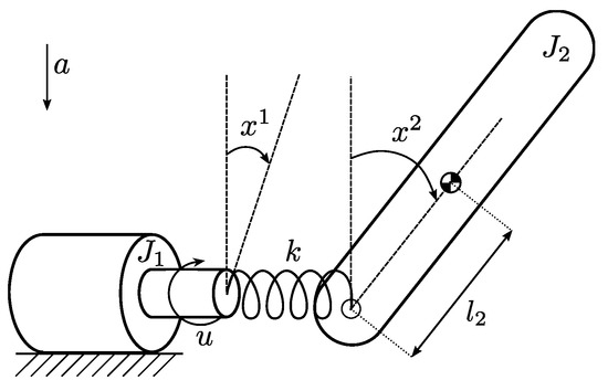
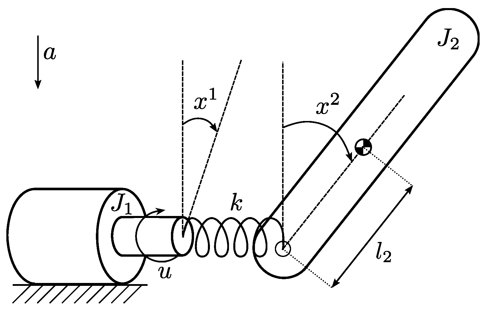
The single link manipulator with joint flexibility consist of two rigid bodies, the base and one link, interconnected by one rotary joint undergoing deflection, modeled as a torsional spring with linear characteristics k, and actuated by one electrical motor. The schematic representation of manipulator with flexible joint is depicted in Figure 1. Let $x^1$ and $x^2$ denote the angular position of the motor shaft and link, respectively. Both are assumed to be equal to zero in the upright position. The chosen set of coordinates is imposing the potential energy to be equal to $V={\displaystyle \frac{1}{2}}k{\left(x^2-x^1\right)}^2+ma{l}_{2}cos{x}^2$, where the mass of the link is m, a stands for gravitational acceleration, and the distance from the joint to the link center of mass is $l_2$ (see Figure 1). The kinetic energy reads $T={\displaystyle \frac{1}{2}}{J}_1{\left({\dot{x}}^1\right)}^2+{\displaystyle \frac{1}{2}}{J}_2{\left({\dot{x}}^2\right)}^2$, where $J_1$ and $J_2=m{l}_2^2+I_2$ are the inertia of the motor shaft and inertia of the link about the axis of rotation, respectively, and $I_2$ is the moment of inertia of the link for pivot point at its mass center.

Figure 1. The single link manipulator with flexible joint.

From Euler-Lagrange formulation we get the dynamics of the system as

$$\begin{array}{c}\hfill \begin{array}{c}\hfill J_1{\ddot{x}}^1-k\left(x^2-x^1\right)=u,\\ \hfill J_2{\ddot{x}}^2-ma{l}_{2}sin{x}^2+k\left(x^2-x^1\right)=0.\end{array}\end{array}$$

(10)

Note that, in this example, the two dimensional configuration manifold is a surface $Q={\mathbb{R}}^2$. Both configurations $x^1$ and $x^2$ physically represent angles (hinting ${\mathbb{S}}^1\times {\mathbb{S}}^1$), nevertheless it is clear that the Equation (10) is not symmetric with respect to $mod\left(2\pi \right)$, i.e., the solution of (10) differs when replacing $x^i$ by $x^i\pm 2c\pi$, for $i=1,2$, and $c\in \mathbb{N}$.

The system (10) takes the form of $\left(\mathcal{MS}\right)$ given by (2), defined on $\mathrm{T}Q={\mathbb{R}}^2\times {\mathbb{R}}^2={\mathbb{R}}^4$,

$$\begin{array}{c}\hfill \begin{array}{cc}\hfill {\dot{x}}^1& =v^1\hfill \\ \hfill {\dot{v}}^1& =e^1\left(x\right)+{\displaystyle \frac{1}{J_1}}u,\mathrm{where}:e^1\left(x\right)={\displaystyle \frac{k\left(x^2-x^1\right)}{J_1}},\hfill \\ \hfill {\dot{x}}^2& =v^2\hfill \\ \hfill {\dot{v}}^2& =e^2\left(x\right),\mathrm{where}:e^2\left(x\right)={\displaystyle \frac{ma{l}_2}{J_2}}sin{x}^2-{\displaystyle \frac{k}{J_2}}\left(x^2-x^1\right).\hfill \end{array}\end{array}$$

(11)

Obviously, the FLEX system is already in form (6), since $(x,v)$ constitute the coordinate system, where all Christoffel symbols are zero. Thus condition (7) is trivially satisfied, since $\mathrm{ann}\mathcal{G}=\mathrm{span}\left\{d{x}^2\right\}$ is clearly a subset of $\mathrm{ann}{\mathrm{\Gamma }}_{jk}=\mathrm{span}\left\{d{x}^1,d{x}^2\right\}={\mathbb{R}}^2$.

Global Stabilization Problem

The system is, in fact, MF-linearizable, cf. [5]. Thus, we construct a stabilizer using linearizing coordinates and cascade controller composed of: feedback linearization (inner loop) and linear state feedback (outer loop). Specifically, we first determine the linearizing change of coordinates, then solve the stabilization problem in the resulting linear coordinates, and finally map the solution (i.e., the control law) back into the original coordinates. It is straightforward to verify that the following mechanical change of coordinates (cf. [5])

$$\begin{array}{c}\hfill \begin{array}{cc}\hfill {\tilde{x}}^1& =e^2\left(x\right)={\displaystyle \frac{ma{l}_2}{J_2}}sin{x}^2-{\displaystyle \frac{k}{J_2}}(x^2-x^1)\hfill \\ \hfill {\tilde{v}}^1& ={\displaystyle \frac{\partial e^2\left(x\right)}{\partial x^2}}{v}^2+{\displaystyle \frac{\partial e^2\left(x\right)}{\partial x^1}}{v}^1={\displaystyle \frac{ma{l}_2}{J_2}}cos\left(x^2\right)v^2+{\displaystyle \frac{k}{J_2}}\left(v^1-v^2\right),\hfill \\ \hfill {\tilde{x}}^2& =x^2\hfill \\ \hfill {\tilde{v}}^2& =v^2,\hfill \end{array}\end{array}$$

(12)

yields the linear system

$$\begin{array}{cc}\hfill {\dot{\tilde{x}}}^1=& {\displaystyle \frac{ma{l}_2}{J_2}}{v}^{2}cos{x}^2-{\displaystyle \frac{k}{J_2}}(v^2-v^1)={\tilde{v}}^1\hfill \\ \hfill {\dot{\tilde{v}}}^1=& {\displaystyle \frac{1}{J_2^2}}\left(ma{l}_{2}cos{x}^2-k\right)\left(ma{l}_{2}sin{x}^2-k(x^2-x^1)\right)+\hfill \\ \hfill +& {\displaystyle \frac{k^2}{J_1{J}_2}}(x^2-x^1)-{\displaystyle \frac{ma{l}_2}{J_2}}{\left(v^2\right)}^{2}sin{x}^2+{\displaystyle \frac{k}{J_1{J}_2}}u=\tilde{u},\hfill \\ \hfill {\dot{\tilde{x}}}^2=& v^2={\tilde{v}}^2\hfill \\ \hfill {\dot{\tilde{v}}}^2=& e^2\left(x\right)={\tilde{x}}^1.\hfill \end{array}$$

Clearly, the above linearization is global. The above change of coordinates is continuously differentiable bijection defined globally from ${\mathbb{R}}^4$ onto ${\mathbb{R}}^4$ with the differentiable inverse, i.e., a global diffeomorphism. Moreover, the feedback map $u\mapsto \tilde{u}$ is also defined globally as a mapping $\mathbb{R}\to \mathbb{R}$. This, in turn, yields a global equivalence of trajectories: it establishes a one-to-one correspondence between the trajectories $z(t,z_0,u)$ of the original system (11) (written as $\dot{z}=F\left(z\right)+G\left(z\right)u$) and those of the linearized system $\tilde{z}(t,{\tilde{z}}_0,\tilde{u})$, given by (12). Recall that $z=(x,v)$ are the coordinates in $\mathrm{T}Q$, while $z_0$ and ${\tilde{z}}_0$ denote the corresponding initial conditions.

As stated in Definition 2, the stabilization goal is $z_0=(x_0,v_0)=(0,0)$ which corresponds to the point ${\tilde{z}}_0=({\tilde{x}}_0,{\tilde{v}}_0)=(0,0)$ in the linearizing coordinates. Therefore, by enforcing ${\tilde{z}}_0$ to be a globally stable equilibrium of the closed-loop linearized system, we achieve global stabilization of the original nonlinear system.

The system expressed in new coordinates simplifies to trivial chain of integrators. Such a form significantly simplifies the control design, as it decouples the nonlinear dynamics of the original system and allows the use of linear control techniques to achieve desired performance. We choose a simple state feedback, i.e.,

$$\tilde{u}=-k_1{\tilde{x}}^1-k_2{\tilde{v}}^1-k_3{\tilde{x}}^2-k_4{\tilde{v}}^2,$$

(13)

where $k_i$ for $i=1,\dots ,4$ denote gains of linear state-feedback. Thus, the control signal applied to the original system (11) takes the following form

$$\begin{array}{c}\hfill \begin{array}{cc}\hfill u& =p_1{x}^1-p_1{x}^2+p_{2}sin{x}^2-p_2{x}^{1}cos{x}^2+p_2{x}^{2}cos{x}^2+\hfill \\ \hfill & -p_{3}sin{x}^{2}cos{x}^2+p_4{\left(v^2\right)}^{2}sin{x}^2+p_5\tilde{u},\hfill \end{array}\end{array}$$

(14)

where $p_1={\displaystyle \frac{k(J_1+J_2)}{J_2}}$, $p_2={\displaystyle \frac{J_{1}ma{l}_2}{J_2}}$, $p_3={\displaystyle \frac{J_1{\left(ma{l}_2\right)}^2}{k{J}_2}}$, $p_4={\displaystyle \frac{J_{1}ma{l}_2}{k}}$, and $p_5={\displaystyle \frac{J_1{J}_2}{k}}$.

For simulation, we are setting the parameters of the manipulator as: $m=0.5$ [kg], $l_1=0.5$ [m], $J_1=4·{10}^{-3}$ [kg·m²], $J_2=3·{10}^{-3}$ [kg·m²], $a=9.81$ [m/s²], $k=2$ [N/m]. Different initial conditions are examined in the sets $x^1\left(0\right)\in \{-\pi ,\pi \}$ and $x^2\left(0\right)\in \{-\pi ,\pi \}$. The gains of stabilizer are chosen to fulfill several requirements. (1) The gains $k_1$ and $k_3$ should ensure the stabilization of closed loop (9) of the FLEX system [2]. (2) The gains $k_2$ and $k_4$ are chosen to be strictly dissipative. (3) All gains should stabilize the 4th order system, i.e., $k_1{k}_2{k}_4>k_4^2+k_2^2{k}_3$ [23]. Here, we choose $k_1=6{\zeta }^2$, and $k_2=4\zeta$, $k_3={\zeta }^4$, $k_4=4{\zeta }^3$, for $\zeta =15$.

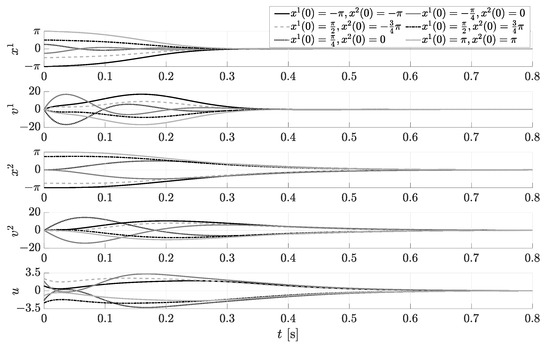
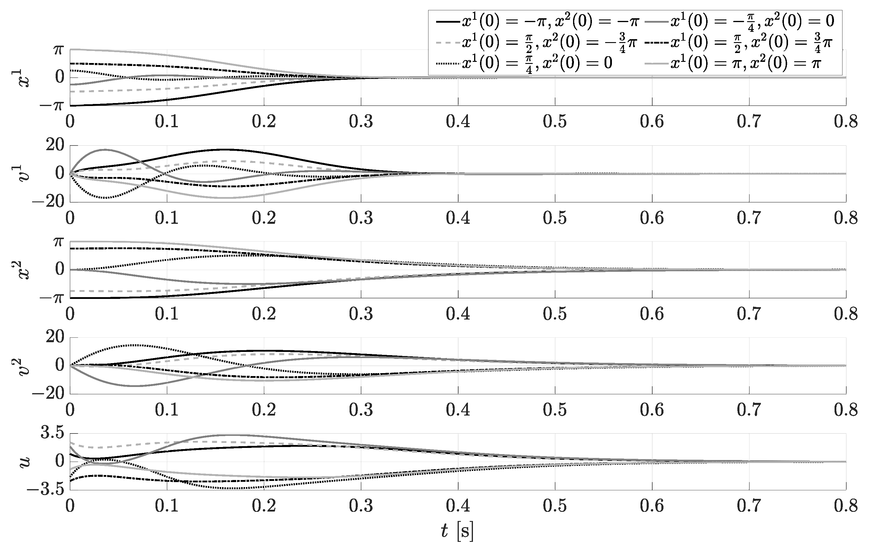
Several example results are gathered in Figure 2. Each line represents a trajectory corresponding to different initial conditions for the configuration coordinates (the initial velocities are always assumed to be zero), as indicated in the legend of Figure 2. Clearly, the equilibrium configuration is (practically) reached in finite time, independently of initial condition. The system lacks singularities, therefore control signal is limited.

Figure 2. Simulation results of FLEX system (11) with cascade controller: inner (linearization loop) (14) and outer (state feedback) (13), under different initial conditions.

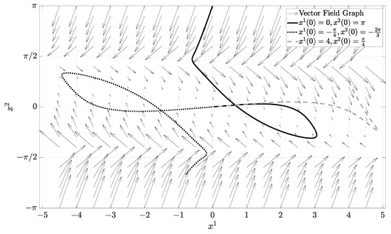
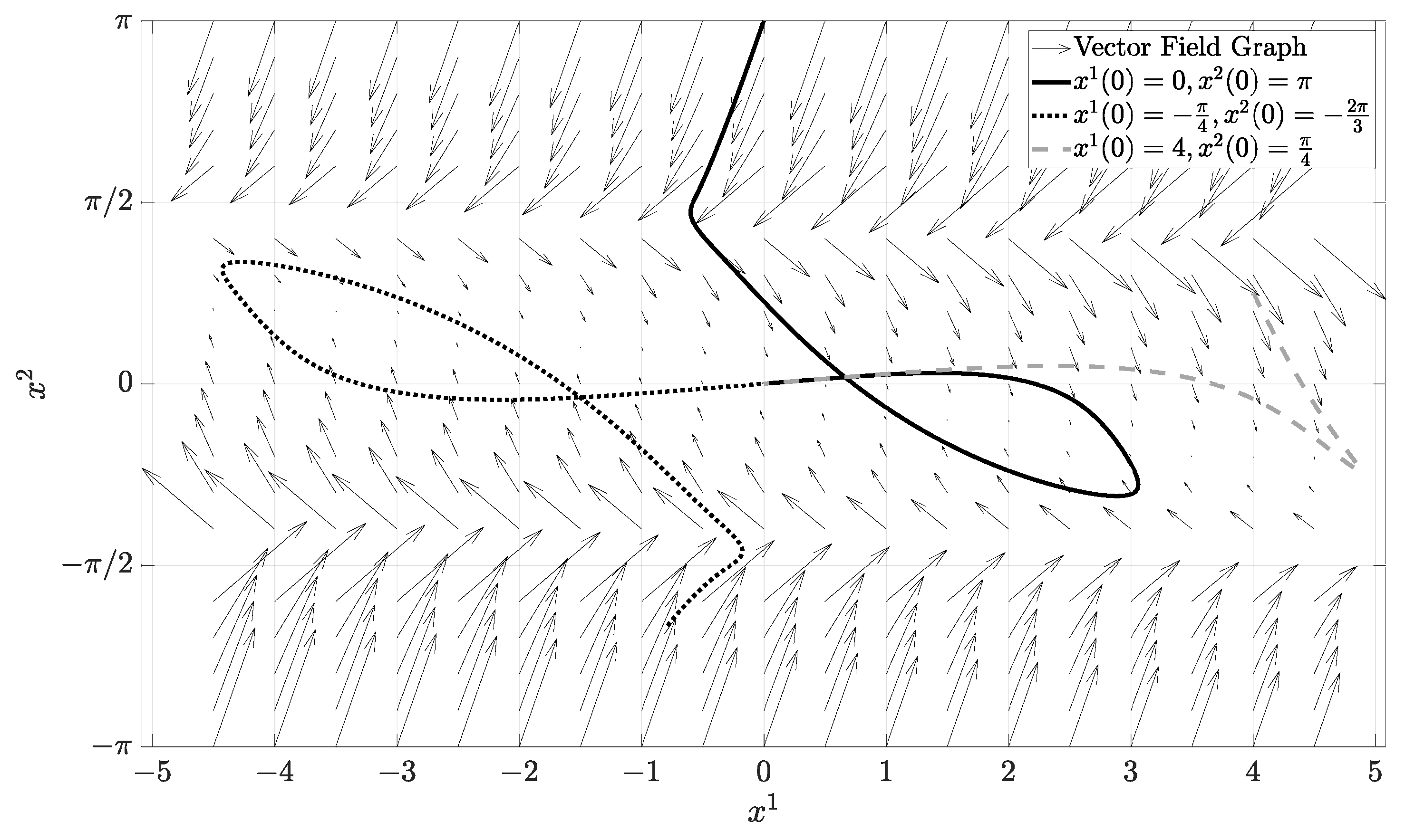
Moreover, in Figure 3 we present a vector field of the closed-loop system $\dot{z}=F_c\left(z\right)$, together with exemplary configuration trajectories starting from different initial conditions, as explained in the legend of Figure 3. Although the system has 4 state variables we project the trajectory to the configuration manifold, i.e., $\mathrm{\Pi }\left(z(t,z_0,u)\right)=x(t,x_0,u)$, where $z_0=(x_0,0)$ and $\mathrm{\Pi }:\mathrm{T}Q\to Q$, $\mathrm{\Pi }\left(z\right)=x$ is the canonical projection, which assigns to the pair $(x,v)$ the point x at which the velocity v is attached.

Figure 3. Vector field graph and example trajectories of closed-loop FLEX system (11) with cascade controller (13) and (14), projected on configuration manifold.

The MF-linearized FLEX system has one vortex at origin, as clearly depicted in Figure 3. The arrows are pointing towards the equilibrium point $x_{eq}^1=x_{eq}^2=0$, independently of initial configuration. It is possible to alter the orientation of quivers by changing tuning parameters $k_i$. Particularly, bigger gain values will cause the arrows to be more vertical, and the resulting trajectory to reach equilibrium faster.

4.2. Inertia Wheel Pendulum (IWP)

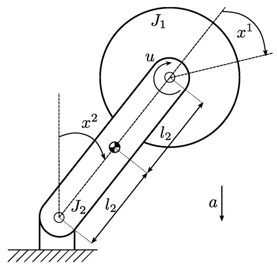
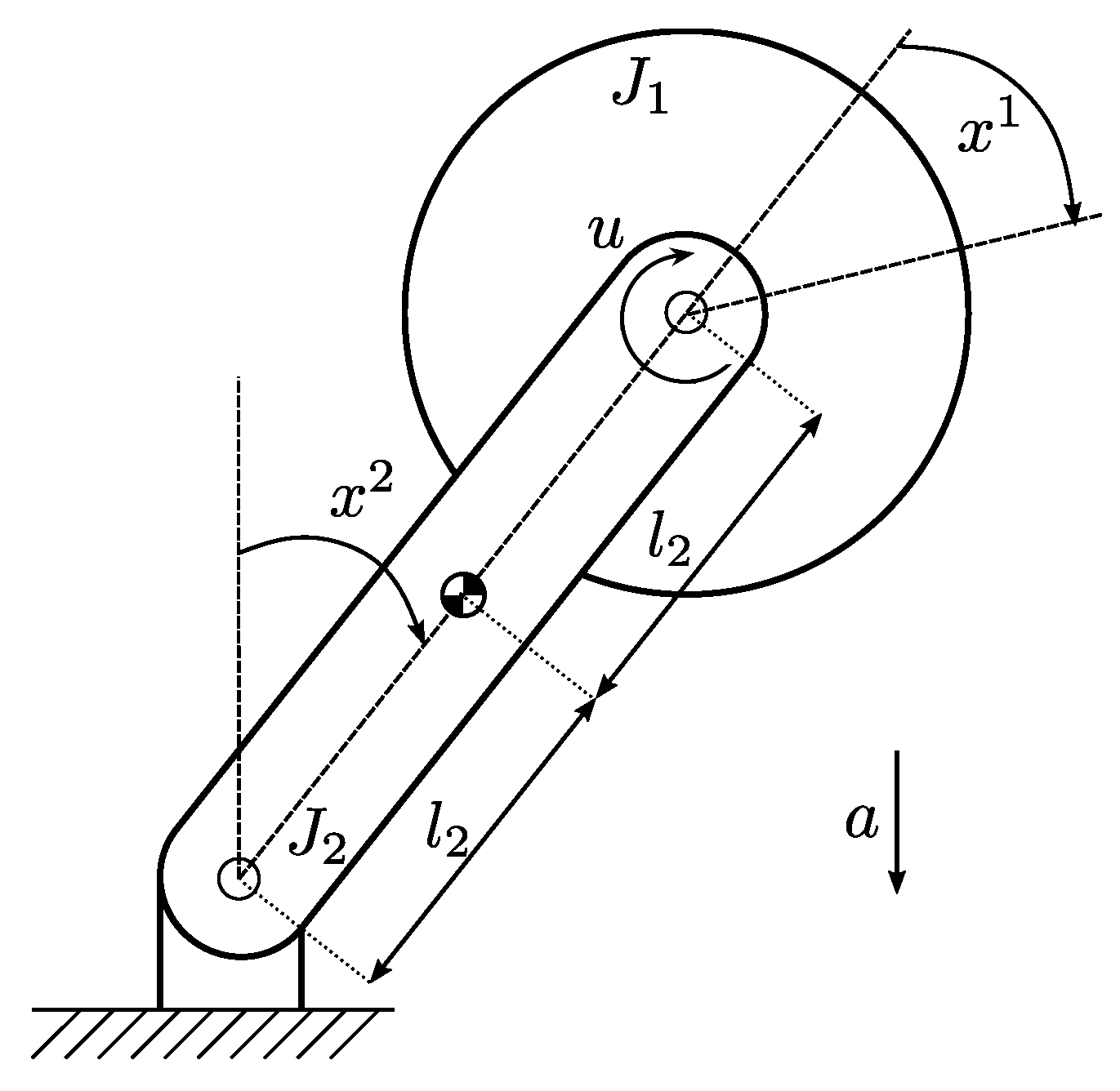
Consider the Inertia Wheel Pendulum [24,25]. It is an inverted pendulum with a rotating wheel at the end. Let $x^1$ denote the angle of the wheel and $x^2$ is the angle of the pendulum (see Figure 4). Both angles are chosen to be zero at the upright position. The configuration manifold is the torus $Q={\mathbb{S}}^1\times {\mathbb{S}}^1$. The chosen set of coordinates is imposing the potential energy to be equal to $V=\left(2m_1{l}_2+m_2{l}_2\right)acos{x}^2$, where a stands for gravitational acceleration, the masses of the wheel and the pendulum are $m_1,m_2$ and the distance from the joint to the link center of mass is $l_2$. Note that, the pendulum mass center is at the geometrical center, therefore the length of the link reads $2l_2$. The kinetic energy is the sum of kinetic energies of both, wheel and pendulum, i.e., $T={\displaystyle \frac{1}{2}}{m}_1{\left(2l_2\right)}^2+{\displaystyle \frac{1}{2}}{I}_1{({\dot{x}}^1+{\dot{x}}^2)}^2+{\displaystyle \frac{1}{2}}{J}_2{\left({\dot{x}}^2\right)}^2$, where $J_2=m_2{l}_2^2+I_2$ is the inertia of the pendulum about the axis of rotation, and $I_1,I_2$ are the momenta of inertia of the wheel and pendulum for pivot point at its mass center. From Euler-Lagrange formulation we get the dynamics of the system as

$$\begin{array}{c}\hfill \begin{array}{c}\hfill I_1\left({\ddot{x}}^1+{\ddot{x}}^2\right)=u,\\ \hfill I_1{\ddot{x}}^1+(J_1+J_2){\ddot{x}}^2-m_{0}sin{x}^2=0,\end{array}\end{array}$$

(15)

where $J_1=m_1{\left(2l_2\right)}^2+I_1$, with constant parameter $m_0=a\left(2m_1{l}_2+m_2{l}_2\right)$. The only control of the system is a torque applied to the wheel, so the system is underactuated. The equations of $\left(\mathcal{MS}\right)$ are:

$$\begin{array}{c}\hfill \begin{array}{cc}\hfill {\dot{x}}^1& =v^1\hfill \\ \hfill {\dot{v}}^1& =e^1+g^{1}u,\mathrm{where}:e^1=-{\displaystyle \frac{m_0}{m_d}}sin{x}^2,g^1={\displaystyle \frac{I_1+m_d}{I_1{m}_d}},\hfill \\ \hfill {\dot{x}}^2& =v^2\hfill \\ \hfill {\dot{v}}^2& =e^2+g^{2}u,\mathrm{where}:e^2={\displaystyle \frac{m_0}{m_d}}sin{x}^2,g^2=-{\displaystyle \frac{1}{m_d}},\hfill \end{array}\end{array}$$

(16)

with constant parameter $m_d=\left(m_1{\left(2l_2\right)}^2+J_2\right)$. Obviously, the IWP system is already in (6) form, since $(x,v)$ are the coordinate system, where all Christoffel symbols are zero, thus condition (7) is trivially satisfied, analogously as in the previous example.

Figure 4. The Inertia Wheel Pendulum.

Stabilization Problem

The system is MF-linearizable [18], thus, analogously to the previous example, we will construct a stabilizer using linearizing coordinates. We propose the following transformation

$$\begin{array}{c}\hfill \begin{array}{cc}\hfill {\tilde{x}}^1& =x^1+{\displaystyle \frac{m_d+I_1}{I_1}}{x}^2\hfill \\ \hfill {\tilde{v}}^1& =v^1+{\displaystyle \frac{m_d+I_1}{I_1}}{v}^2,\hfill \\ \hfill {\tilde{x}}^2& ={\displaystyle \frac{m_0}{I_1}}sin{x}^2\hfill \\ \hfill {\tilde{v}}^2& ={\displaystyle \frac{m_0}{I_1}}cos{x}^2{v}^2,\hfill \end{array}\end{array}$$

(17)

together with the feedback action $\tilde{u}=-{\displaystyle \frac{m_0}{I_1}}sin{x}^2{\left(v^2\right)}^2+{\displaystyle \frac{m_0^2}{I_1{m}_d}}sin{x}^{2}cos{x}^2-{\displaystyle \frac{m_0}{I_1{m}_d}}cos{x}^{2}u$ to MF-linearize the system, which in new coordinates reads

$$\begin{array}{c}\hfill {\dot{\tilde{x}}}^1={\tilde{v}}^1{\dot{\tilde{v}}}^1={\tilde{x}}^2{\dot{\tilde{x}}}^1={\tilde{v}}^2{\dot{\tilde{v}}}^2=\tilde{u}.\end{array}$$

The system expressed in new coordinates simplifies to trivial chain of integrators. Once again we propose to apply simple state feedback, i.e.,

$$\tilde{u}=-k_1{\tilde{x}}^1-k_2{\tilde{v}}^1-k_3{\tilde{x}}^2-k_4{\tilde{v}}^2,$$

(18)

to control the linearized system. Note that, both diffeomorphism (17) and the control signal

$$u=-m_d{\displaystyle \frac{sin{x}^2}{cos{x}^2}}{\left(v^2\right)}^2+m_{0}sin{x}^2-{\displaystyle \frac{m_d{I}_1}{m_{0}cos{x}^2}}\tilde{u}$$

(19)

impose the above linearization to be local. The change of coordinate ${\tilde{x}}^2={\displaystyle \frac{m_0}{I_1}}sin{x}^2$ in (17) is periodic, so it is one-to-one only on certain intervals, which are defined by singularities due to division by $cos{x}^2$ in (19). The configuration space is divided into two subsets, by two singular configurations i.e., for $x^2=\pm {\displaystyle \frac{\pi }{2}}$. Therefore, the diffeomorphism (17) works in two domains: $Q^{\prime }=\{x^1\in {\mathbb{S}}^1,x^2\in [-{\displaystyle \frac{\pi }{2}},{\displaystyle \frac{\pi }{2}}\left]\right\}$ and $Q^{\prime \prime }=\{x^1\in {\mathbb{S}}^1,x^2\in [-\pi ,-{\displaystyle \frac{\pi }{2}}[\cup ]{\displaystyle \frac{\pi }{2}},\pi \left]\right\}$. Each domain has its unique equilibrium point, given by $x_{eq}^1=v_{eq}^1=x_{eq}^2=v_{eq}^2=0$ and $x_{eq}^1=-{\displaystyle \frac{m_d+I_1}{I_1}}\pi$, $x_{eq}^2=\pi$, $v_{eq}^1=v_{eq}^2=0$, for $Q^{\prime }$ and $Q^{\prime \prime }$ respectively, see [17].

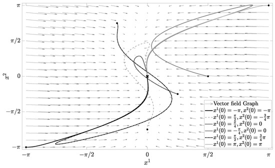
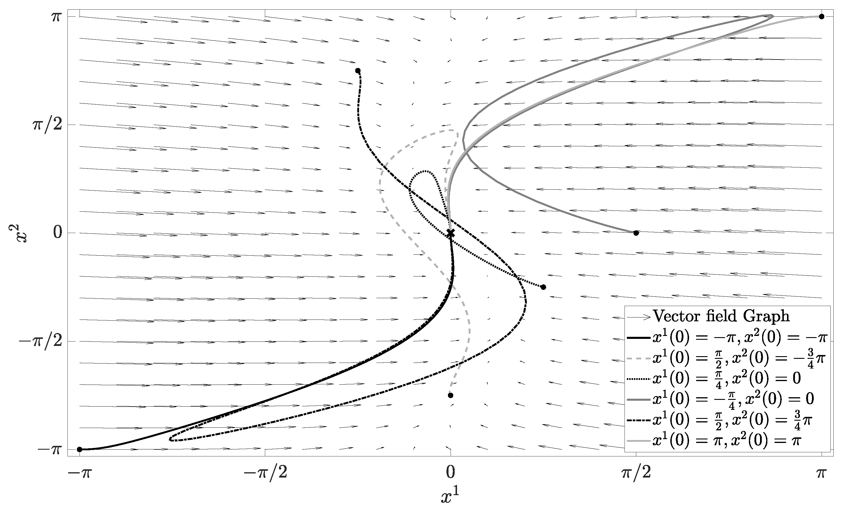
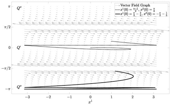
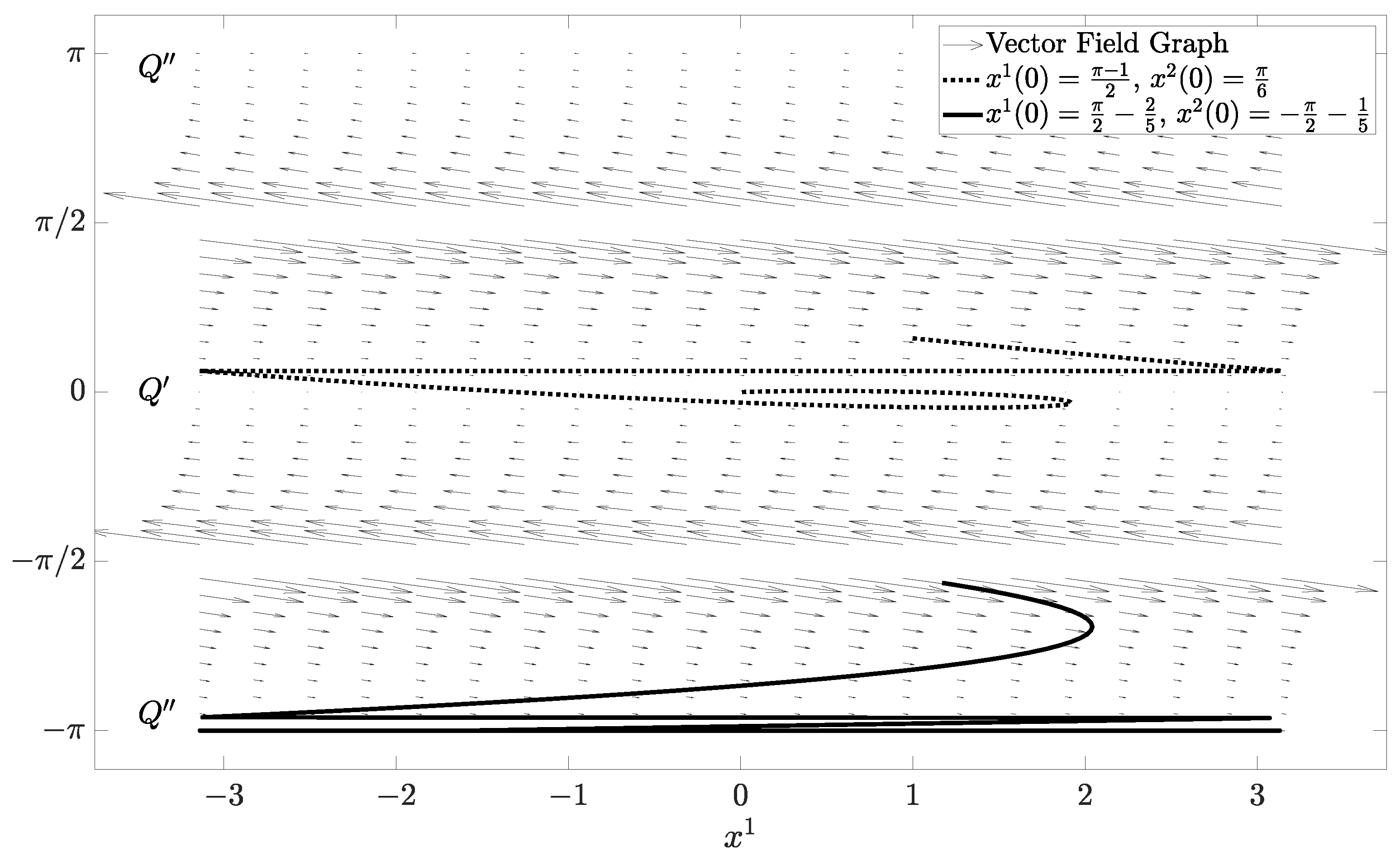
Therefore, feedback controller (18) stabilizes the original system (16) at different equilibrium point, depending on the initial condition, whether it is in domain $Q^{\prime }$ or $Q^{\prime \prime }$ (see Figure 5). Both domains exist independently and are not distinguished by MF-linearized system.

Figure 5. Vector field graph and example trajectories of closed-loop IWP system (16) with cascade controller (18) and (19), projected on configuration manifold.

For simulation, we are setting the parameters of IWP, c.f. [26], as: $m_1=0.86422$ [kg], $m_2=3.228$ [kg], $l_2=2.6·{10}^{-2}$ [m], $I_1=0.7986·{10}^{-3}$ [kg·m²], $I_2=3.042·{10}^{-2}$ [kg·m²], $a=9.81$ [m/s²]. The stabilizer gains are chosen to guarantee the stability of the closed-loop system (similar reasoning as in Section 4.1) as $k_1={\zeta }^4$, $k_2=4{\zeta }^3$, $k_3=6{\zeta }^2$, and $k_4=4\zeta$, for $\zeta =2$. The control signal (19) is limited by symmetric bounds $u_{max}=10$, i.e., $\mathrm{sat}\left(u\right)=max(-u_{max},min(u,u_{max}))$. Actuator saturation is enforced to guarantee practical implementability, contrast to works using saturated controls [27]. This type of saturation is natural in practical implementations and can be interpreted as, for example, a bound on the motor drive voltage, reflecting inherent actuator limitations.

Different initial conditions are examined in the sets $x^1\left(0\right)\in \{-\pi ,\pi \}$ and $x^2\left(0\right)\in \{-\pi ,\pi \}$. The vector field graph is constructed for closed loop system, with $v^1\left(0\right)=v^2\left(0\right)=0$ for visualization purposes, as shown in Figure 5.

The arrows are denoting the velocities of the system at a given configuration. Few interesting characteristics of the system can be noticed. First, if $x^2\left(0\right)\in Q^{\prime }$ the vector field creates a vortex pushing the system to its origin, as expected. Second, if $x^2\left(0\right)\in Q^{\prime \prime }$ the vector field pushes the system to the other equilibrium point $x_{eq}^2=\pi$. Third, the arrows close to the singularity configuration, for which the control signal (19) tends to infinity, are pointing at the opposite directions, indicating the separate characteristics of both domains.

According to the reasoning presented above, the MF-linearized system exist separately on two domains. As a result it is not possible to force the MF-linearized system to stabilize at the origin if $x^2\left(0\right)\in Q^{\prime \prime }$, see example trajectory of IWP system in Figure 5. The linearization is local and is imposing to limit the $x^2$ to $\left[-{\displaystyle \frac{\pi }{2}},{\displaystyle \frac{\pi }{2}}\right]$.

To address the problem of separate domains of linearized IWP model we propose to switch the control signal when the system is in domain $Q^{\prime \prime }$. Natural question arises, of how to choose the new control signal.

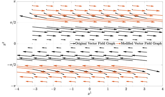
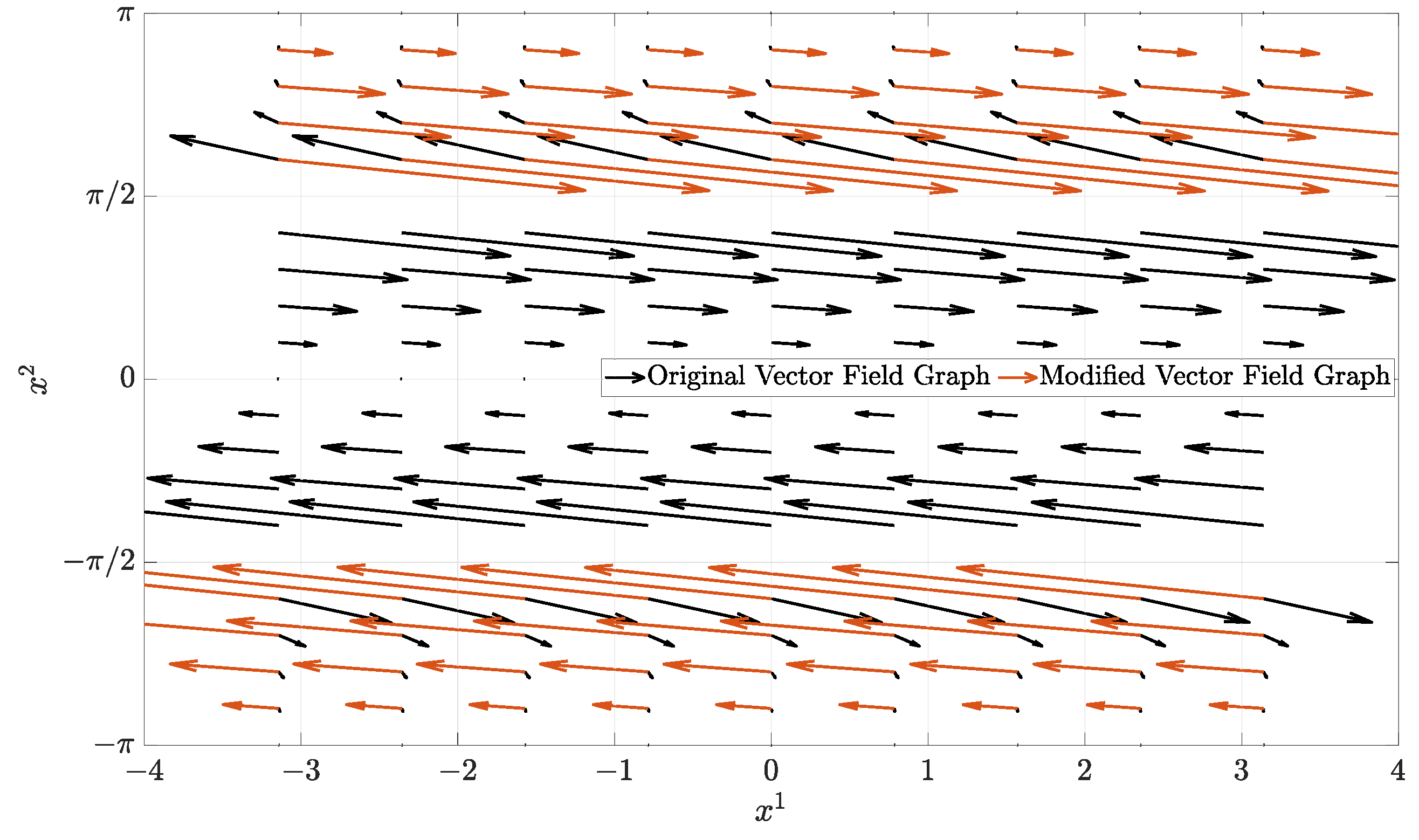
We can conclude that, to be able to globally stabilize the system at its origin, vector field graph must fulfill the following conditions: (1) if $x^2\in Q^{\prime }$ the vector field should create a vortex pushing the system to its origin, (2) if $x^2\in Q^{\prime \prime }$ the vector field should point towards $Q^{\prime }$, (3) the arrows at the junction of the domains (singularity configuration) should point in the same direction, in both domains.

Taking into account the above assumptions, we propose the following simple switching logic of the control signal:

$$\tilde{u}=\left\{\begin{array}{cc}-k_1{\tilde{x}}^1-k_2{\tilde{v}}^1-k_3{\tilde{x}}^2-k_4{\tilde{v}}^2,& \mathrm{if}{x}^2\in Q^{\prime }\\ k_1{\tilde{x}}^1+k_2{\tilde{v}}^1+k_3{\tilde{x}}^2+k_4{\tilde{v}}^2,& \mathrm{if}{x}^2\in Q^{\prime \prime }.\end{array}\right.$$

(20)

The proposed solution is changing the vector field graph of the closed loop system, as shown in Figure 6, therefore all of the above conditions are met. Due to the change in the vector field induced by the proposed switching logic, the direction of the quivers becomes consistent on both sides of the singularity, effectively aligning the local vector fields toward the same convergence direction. This alignment eliminates opposing flow behavior that would otherwise trap trajectories near the singularity. Furthermore, when saturation is applied to the control signal, the system is able to smoothly traverse the singular region rather than being constrained by control discontinuities. As a result, the state trajectories pass through the singularity and continue toward the global equilibrium point.

Figure 6. Vector field graph of closed-loop IWP system (16) with cascade controller, i.e., inner (linearization loop) (19) and outer: original state feedback (18) (in black) or modified state feedback (20) (in red), projected on configuration manifold.

Another explanation is related to the stability of the system. Since, by design, we intend to force the system not to stabilize at equilibrium point $x_{eq}^2=\pi$, the domain $Q^{\prime \prime }$ which includes that point, is unstable, due to positive control signal. Therefore, we are forcing the system not to stabilize at undesired equilibrium.

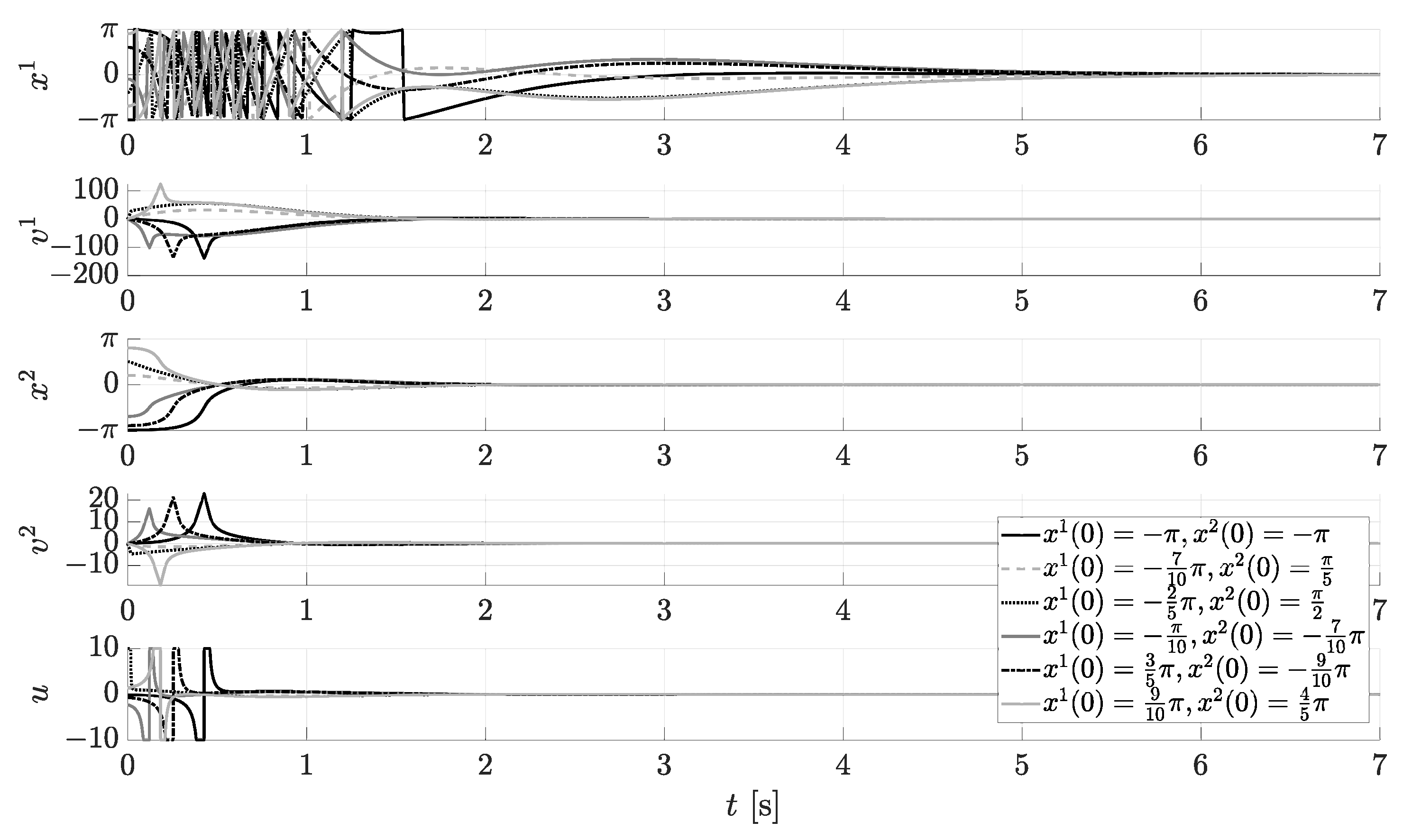
The closed loop system with applied switching logic (20) is examined for the same set of initial conditions as before and the results of such are depicted in Figure 7. The basic conclusion is that a MF-linearized IWP system with proposed switching logic is globally stabilized at $x_{eq}^1=v_{eq}^1=x_{eq}^2=v_{eq}^2=0$.

Figure 7. Simulation results of IWP system (16) with cascade controller: inner (19) and outer (20), under different initial conditions.

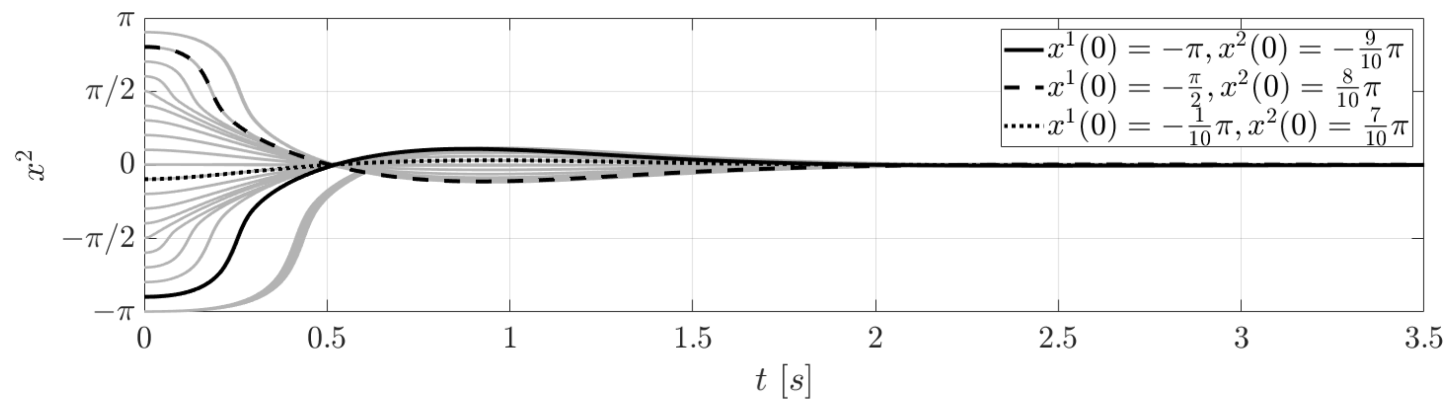
To further illustrate the convergence properties of the proposed switching logic, Figure 8 presents the evolution of the state variable $x^2$ for multiple initial conditions. Each trajectory, depicted in gray, corresponds to a distinct initial state, while three representative trajectories are highlighted in color for clarity. It is observed that all trajectories exhibit convergence toward the equilibrium $x_{eq}^2=0$, regardless of the initial value. This consistent behavior confirms the global stability of the closed-loop system and demonstrates the robustness of the switching control law in driving the system states to the desired equilibrium.

Figure 8. $x^2$ coordinate for IWP system (16) with cascade controller (19) and (20), under various initial conditions.

4.3. Inverted Pendulum on a Cart (IPC)

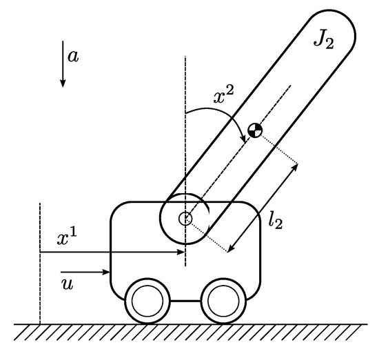
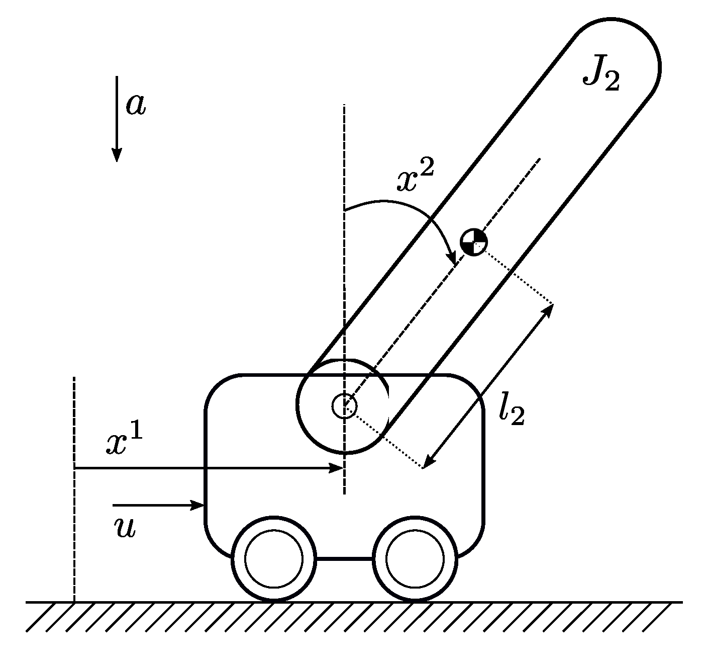
Consider Inverted Pendulum on a Cart system [28,29,30]. The system consists of a pendulum mounted on a cart that can translate along a horizontal track and is controlled by the force u produced by a motor. The pendulum is free to rotate in the vertical plane, with its upright configuration corresponding to the unstable equilibrium, and with positive values indicating the clockwise rotation of the pendulum. Let $x^1$ denote horizontal position of the cart along the track and $x^2$ angular position of the pendulum, as depicted in Figure 9. The chosen set of coordinates is imposing the potential energy to be equal to $V=m_2{l}_{2}acos{x}^2$, where a stands for gravitational acceleration, $m_2$ is the mass of the pendulum, and the distance from the joint to the link center of mass is $l_2$. The kinetic energy reads $T={\displaystyle \frac{1}{2}}\left(m_1+m_2\right){\dot{x}}_1^2+m_2{l}_2{\dot{x}}^1{\dot{x}}^{2}cos{x}^2+{\displaystyle \frac{1}{2}}{m}_2{l}_2^2{\dot{x}}_2^2+{\displaystyle \frac{1}{2}}{I}_2{\dot{x}}_2^2$, where $m_1$ stands for the mass of the cart, $I_2$ is the moment of inertia of the pendulum. From Euler-Lagrange equations we get the dynamics of the system as, cf. e.g., [27,30]:

$$\begin{array}{c}\hfill \begin{array}{cc}\hfill m{\ddot{x}}^1+m_2{l}_2{\ddot{x}}^{2}cos\left(x^2\right)-m_2{l}_2{\left({\dot{x}}^2\right)}^{2}sin\left(x^2\right)& =u,\hfill \\ \hfill J_2{\ddot{x}}^2-m_2{l}_{2}asin\left(x^2\right)+m_2{l}_2{\ddot{x}}^{1}cos\left(x^2\right)& =0,\hfill \end{array}\end{array}$$

(21)

where $m=m_1+m_2$ is the total mass of the system, and $J_2=I_2+m_2{l}_2^2$, according to Steiner’s theorem.

Figure 9. The inverted pendulum on a cart.

Note that, in this example, the two dimensional configuration manifold is $Q={\mathbb{R}}^1\times {\mathbb{S}}^1$, and state-space is the tangent bundle $\mathrm{T}Q=Q\times {\mathbb{R}}^2$.

The system (21) takes the form of $\left(\mathcal{MS}\right)$, cf. e.g., [2,29]:

$$\begin{array}{c}\hfill \begin{array}{cc}\hfill {\dot{x}}^1& =v^1\hfill \\ \hfill {\dot{v}}^1& =-{\mathrm{\Gamma }}_{22}^1\left(x\right)v^2{v}^2+e^1\left(x\right)+g^1\left(x\right)u\hfill \\ \hfill {\dot{x}}^2& =v^2\hfill \\ \hfill {\dot{v}}^2& =-{\mathrm{\Gamma }}_{22}^2\left(x\right)v^2{v}^2+e^2\left(x\right)+g^2\left(x\right)u,\hfill \end{array}\end{array}$$

(22)

where

$$\begin{array}{cc}\hfill & {\mathrm{\Gamma }}_{22}^1\left(x\right)={\displaystyle \frac{-m_2{l}_2{J}_{2}sin\left(x^2\right)}{m{J}_2-m_2^2{l}_2^2{cos}^2\left(x^2\right)}},{\mathrm{\Gamma }}_{22}^2\left(x\right)={\displaystyle \frac{m_2^2{l}_2^{2}sin\left(x^2\right)cos\left(x^2\right)}{m{J}_2-m_2^2{l}_2^2{cos}^2\left(x^2\right)}},\hfill \\ \hfill & e^1\left(x\right)={\displaystyle \frac{-m_2^2{l}_2^{2}asin\left(x^2\right)cos\left(x^2\right)}{m{J}_2-m_2^2{l}_2^2{cos}^2\left(x^2\right)}},e^2\left(x\right)={\displaystyle \frac{m_2{l}_{2}masin\left(x^2\right)}{m{J}_2-m_2^2{l}_2^2{cos}^2\left(x^2\right)}},\hfill \\ \hfill & g^1\left(x\right)={\displaystyle \frac{J_2}{m{J}_2-m_2^2{l}_2^2{cos}^2\left(x^2\right)}},g^2\left(x\right)={\displaystyle \frac{-m_2{l}_{2}cos\left(x^2\right)}{m{J}_2-m_2^2{l}_2^2{cos}^2\left(x^2\right)}}.\hfill \end{array}$$

$\left(\mathcal{CNS}\right)$ and Stabilization Problem

We compute a covector $\omega \in \mathrm{ann}\mathcal{G}$ to be $\omega =J_{2}d{x}^1+m_2{l}_{2}cos\left(x^2\right)d{x}^2$. The only nonzero ${\mathrm{\Gamma }}_{jk}$ is ${\mathrm{\Gamma }}_{22}={\mathrm{\Gamma }}_{22}^1{\displaystyle \frac{\partial }{\partial x^1}}+{\mathrm{\Gamma }}_{22}^2{\displaystyle \frac{\partial }{\partial x^2}}$. A direct calculation show that ${\omega }_i{\mathrm{\Gamma }}_{22}^i=0$ thus condition (7) is satisfied. Consequently, by Proposition 1, there exists a pure mechanical feedback that transforms the system into $\left(\mathcal{CNS}\right)$ given by (6). We apply MF-feedback of the form (5) in order to bring the system into form (6):

$$\begin{array}{cc}\hfill & u={\gamma }_{22}\left(x\right)v^2{v}^2+\alpha \left(x\right)+\beta \left(x\right)\tilde{u},\hfill \end{array}$$

(23)

$$\begin{array}{cc}\hfill \mathrm{where}:& {\gamma }_{22}\left(x\right)=-m_2{l}_{2}sin\left(x^2\right),\hfill \\ \hfill & \alpha \left(x\right)={\displaystyle \frac{{\left(m_2{l}_2\right)}^{2}a}{J_2}}sin\left(x^2\right)cos\left(x^2\right),\hfill \\ \hfill & \beta \left(x\right)=\left(ma-{\displaystyle \frac{{\left(m_2{l}_2\right)}^{2}a}{J_2}}{cos}^2\left(x^2\right)\right).\hfill \end{array}$$

Thus the resultant system reads

$$\begin{array}{c}\hfill \begin{array}{cc}\hfill {\dot{x}}^1& =v^1\hfill \\ \hfill {\dot{v}}^1& =a\tilde{u}\hfill \\ \hfill {\dot{x}}^2& =v^2\hfill \\ \hfill {\dot{v}}^2& ={\displaystyle \frac{m_2{l}_{2}a}{J_2}}sin\left(x^2\right)-{\displaystyle \frac{m_2{l}_{2}a}{J_2}}cos\left(x^2\right)\tilde{u}.\hfill \end{array}\end{array}$$

(24)

In order to stabilize the system (24), we first construct the following control signal

$$\begin{array}{c}\hfill \tilde{u}={\displaystyle \frac{\frac{m_2{l}_{2}a}{J_2}sin\left(x^2\right)+k_1{x}^2+k_2{v}^2+\overline{u}(x,v)}{\frac{m_2{l}_{2}a}{J_2}cos\left(x^2\right)}}.\end{array}$$

(25)

In particular, if $\overline{u}=0$ and tuning parameters $k_1,k_2>0$ are chosen appropriately, such that the $(x^2,v^2)$-subsystem is exponentially stable. Now, it remains to design $\overline{u}(x,v)$ such that it will stabilize $(x^1,v^1)$-subsystem in (24) and will not violate stability of the second subsystem. One can propose, cf. [30],

$$\begin{array}{c}\hfill \overline{u}=-k_1{tan}^{-1}\left(-k_3{x}^1-k_4{v}^1\right),\end{array}$$

(26)

where $k_3$ and $k_4$ are another tuning parameters. The choice of the control signal $\overline{u}$ has three complementary reasons. First, it stabilizes the first subsystem, as for small errors the ${tan}^{-1}$ is linear and the $\overline{u}$ behaves as negative proportional-derivative controller. At the same time, the saturation prevents the $\overline{u}$ from becoming arbitrarily large, the value remains bounded and smooth, even for bigger $|x^1|$ or $|v^1|$. Third, for small values of $k_3$ and $k_4$ the perturbation injected into the second subsystem is small and can be rejected by $x^2$ loop.

Importantly, the tuning parameters of inner loop ($k_1$ and $k_2$) have to be larger than tuning parameters of outer loop ($k_3$ and $k_4$). Following the reasoning presented in Ref. [29], we have chosen $k_1=360,k_2=66,k_3=0.2$, and $k_4=0.3$.

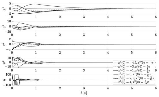
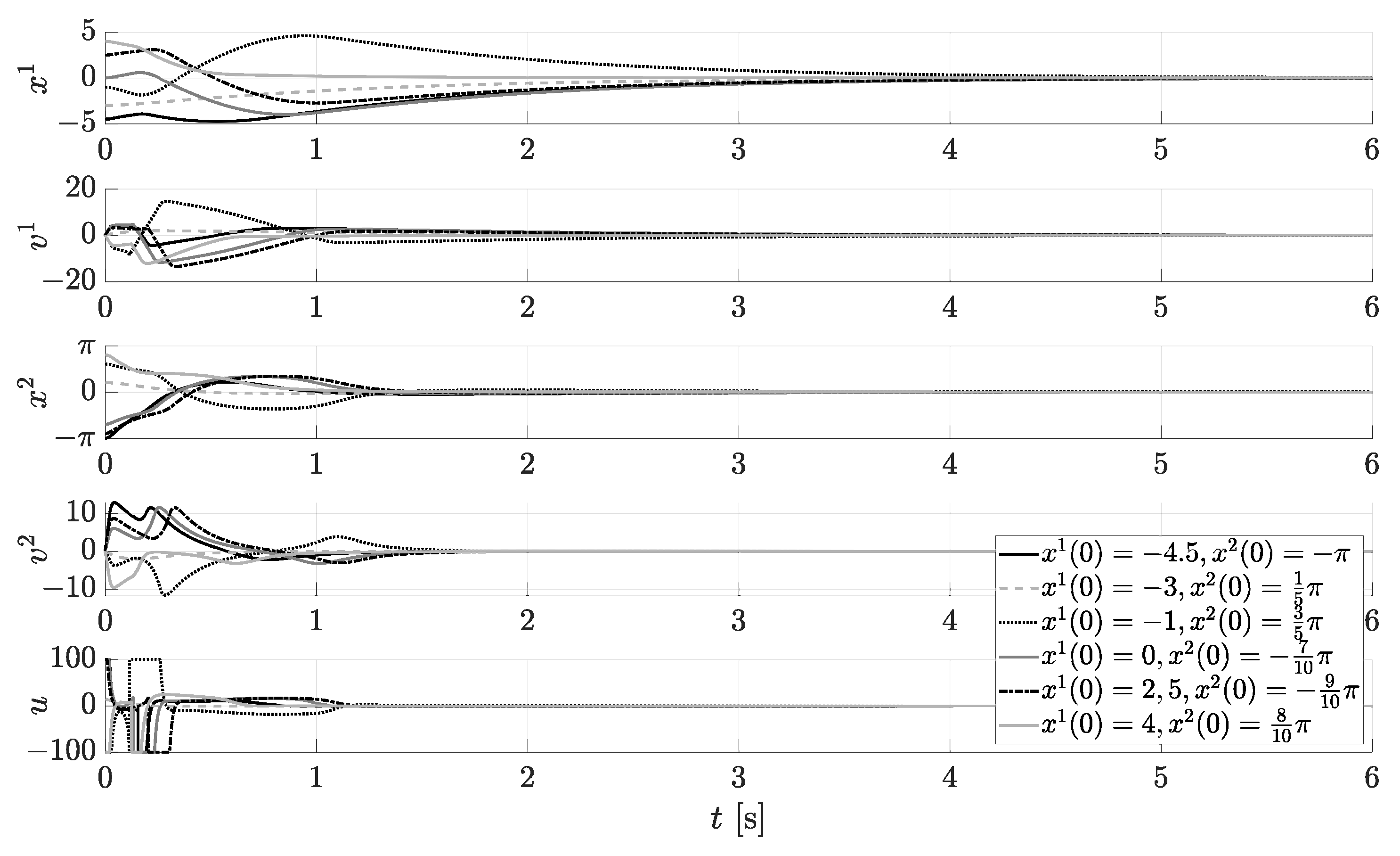
For simulation, we are setting the parameters of IPC, c.f [29], as: $m_1=0.6486$ [kg], $m_2=0.0234$ [kg], $l_2=0.2174$ [m], $J_2=0.0016814$ [kg·m²], $a=9.81$ [m/s²]. The control signal (23) is limited by symmetric bounds $u_{max}=100$. The example results for different initial conditions, for closed-loop system with proposed nonlinear control (25) and (26) are gathered in Figure 10. The simulation results confirm that the proposed nonlinear law successfully stabilizes both loops from a variety of initial states. In the time-series plots all state components $(x,v)$ as well as control input converge to zero for every tested initial condition in $x^1\in \{-5,5\}$, $x^2\in \{-\pi ,\pi \}$.

Figure 10. Simulation results of IPC system (22) with cascade controller: $\left(\mathcal{CNS}\right)$ loop (23), and stabilizer (25) and (26), under different initial conditions.

It is important to note that the control input (25) contains a division by $cos\left(x^2\right)$, which introduces a singularity for $x^2=\pm {\displaystyle \frac{\pi }{2}}$. In the vicinity of these points, the control signal could theoretically become unbounded, leading to numerical or physical instability. However, by applying saturation to the control signal, the magnitude of u is limited, ensuring that the system remains well-behaved even near the singularity.

Moreover, the resulting vector field (shown in Figure 11) is designed such that the quivers on both sides of the singular region point in the same direction, guiding the trajectories smoothly across it. Consequently, despite the theoretical singularity, the closed-loop dynamics remain continuous and the system successfully passes through the singular region, ultimately converging to the global equilibrium at the origin. Here, it is not needed to apply the switching logic (contrary to IWP case), due to nonlinear characteristic of the control signal.

Figure 11. Vector field graph and example trajectories of closed-loop IPC system (22) with cascade controller (23), (25) and (26), projected on configuration manifold.

The degenerate 2D vector field plot was constructed setting all velocities to zero and provides a useful geometric view. The quiver field on the $(x^1,x^2)$ plane points toward the equilibrium and the sample trajectories overlaid on this field follow those flow directions, illustrating the closed-loop stability.

5. Conclusions

In this article, we considered a class of mechanical systems for which we examined the problem of equivalence via pure mechanical feedback to systems that do not possess Christoffel symbols. These systems constitute a generalization of Lagrangian systems with zero curvature evolving on Euclidean space. In our formulation, we retain the original coordinates, as they admit a clear physical interpretation.

For this class of systems, we discuss the problem of (almost) global stabilization, which we address through three examples, employing additional techniques to achieve globality.

In all three examples, the stabilizing controller incorporates an external cascade designed for a fully linearized system (Section 4.1 and Section 4.2) as well as for a partially linearized system (Section 4.3). This controller, implemented in the form of linear state feedback, is responsible for pole placement of the closed-loop linearized system. This demonstrates the systematic nature of the proposed method and its practical relevance, while also suggesting potential directions for further development. Naturally, the linear controller may be replaced by any alternative controller designed for linear systems that guarantees specific qualitative control properties.

In the present study, we do not focus on parameter tuning, robustness analysis (both parametric and structural), or detailed performance evaluation. It is, however, worth emphasizing that in each of the considered cases a freedom of pole placement is available, i.e., the ability to shape the system dynamics, robustness, and other characteristics of the closed-loop behavior. The aforementioned aspects, although of paramount importance in engineering practice, are intentionally left for future research. Conducting a detailed qualitative performance analysis would require the formulation of specific control objectives and performance criteria, which we deliberately avoid in order not to obscure the main contribution of this work. In general, it is well known that the performance characteristics of the obtained solutions are inherited from the linear counterparts of the systems under consideration.

An other natural extension of the considered problem involves allowing for changes of coordinates, which will constitute our future studies.

References

- Bloch, A.M. Nonholonomic Mechanics and Control, 1st ed.; Springer: New York, NY, USA, 2003. [Google Scholar]
- Bullo, F.; Lewis, A.D. Geometric Control of Mechanical Systems, 1st ed.; Springer: New York, NY, USA, 2005. [Google Scholar]
- Nijmeijer, H.; van der Schaft, A.J. Nonlinear Dynamical Control Systems, 1st ed.; Springer: New York, NY, USA, 1990. [Google Scholar]
- Bedrossian, N.S.; Spong, M.W. Feedback linearization of robot manipulators and riemannian curvature. J. Robot. Syst. 1995, 12, 541–552. [Google Scholar] [CrossRef] [Scilit]
- Nowicki, M.; Respondek, W. Mechanical linearization of mechanical control systems without controllability assumption. Automatica 2023, 155, 111098. [Google Scholar] [CrossRef] [Scilit]
- Respondek, W.; Ricardo, S. Equivalence and equivariants of mechanical control systems. In Proceedings of the 50th IEEE Conference on Decision and Control and European Control Conference, Orlando, FL, USA, 12–15 December 2011; pp. 7129–7134. [Google Scholar]
- Bloch, A.M.; Leonard, N.E.; Marsden, J.E. Stabilization of mechanical systems using controlled Lagrangians. In Proceedings of the 36th IEEE Conference on Decision and Control, San Diego, CA, USA, 10–12 December 1997; pp. 2356–2361. [Google Scholar]
- Burkov, I.V. Stabilization of a natural mechanical system without measuring its velocities with application to the control of a rigid body. J. Appl. Math. Mech. 1998, 62, 853–862. [Google Scholar] [CrossRef] [Scilit]
- Bloch, A.M.; Leonard, N.E.; Marsden, J.E. Controlled Lagrangians and the stabilization of mechanical systems. I. The first matching theorem. IEEE Trans. Autom. Control 2000, 45, 2253–2270. [Google Scholar] [CrossRef] [Scilit]
- Bloch, A.M.; Chang, D.E.; Leonard, N.E.; Marsden, J.E. Controlled Lagrangians and the stabilization of mechanical systems. II. Potential shaping. IEEE Trans. Autom. Control 2001, 46, 1556–1571. [Google Scholar] [CrossRef] [Scilit]
- Ortega, R.; Mareels, I.; van der Schaft, A.J.; Maschke, B. Energy shaping revisited. In Proceedings of the IEEE International Conference on Control Applications, Anchorage, AK, USA, 25–27 September 2000; pp. 121–126. [Google Scholar]
- Lee, J.M. Riemannian Manifolds: An Introduction to Curvature, 1st ed.; Springer: New York, NY, USA, 1997. [Google Scholar]
- Bhat, S.; Bernstein, D. A topological obstruction to continuous global stabilization of rotational motion and the unwinding phenomenon. Syst. Control Lett. 2000, 39, 63–70. [Google Scholar] [CrossRef] [Scilit]
- Ricardo, S.; Respondek, W. When is a control system mechanical? J. Geom. Mech. 2010, 2, 265–302. [Google Scholar] [CrossRef] [Scilit]
- Respondek, W.; Ricardo, S. On Linearization of Mechanical Control Systems. IFAC Proc. Vol. 2012, 45, 102–107. [Google Scholar] [CrossRef] [Scilit]
- Floren, M.; Classens, K.; Oomen, T.; Noël, J. Feedback linearisation of mechanical systems using data-driven models. J. Sound Vib. 2024, 577, 118335. [Google Scholar] [CrossRef] [Scilit]
- Nowicki, M.; Respondek, W. Feedback linearizable mechanical systems with rotational DOFs. In Proceedings of the 16th Conference Control in Power Electronics and Electric Drives (SENE 2023), Lodz, Poland, 22–24 November 2023. [Google Scholar]
- Nowicki, M.; Respondek, W. Input-output linearization and decoupling of mechanical control systems. Int. J. Robust Nonlinear Control 2024, 34, 8644–8660. [Google Scholar] [CrossRef] [Scilit]
- Shreyas, N.B.; Diego, D.M.; Banavar, R. Feedback Linearizable Discretizations of Second Order Mechanical Systems using Retraction Maps. In Proceedings of the 2025 European Control Conference (ECC), Thessaloniki, Greece, 24–27 June 2025; pp. 1690–1695. [Google Scholar]
- Spong, M.W. Partial feedback linearization of underactuated mechanical systems. In Proceedings of the IEEE/RSJ International Conference on Intelligent Robots and Systems (IROS’94), Munich, Germany, 12–16 September 1994; pp. 314–321. [Google Scholar]
- Isidori, A. Nonlinear Control Systems, 3rd ed.; Springer: London, UK, 1995. [Google Scholar]
- Jakubczyk, B.; Respondek, W. On linearization of control systems. Bull. Pol. Acad. Sci. Tech. Sci. 1980, 28, 517–522. [Google Scholar]
- Zabczyk, J. Mathematical Control Theory, 2nd ed.; Springer Nature: Cham, Switzerland, 2020. [Google Scholar]
- Ecker, L.; Schlacher, K.; Schöberl, M. Observer Design for an Inertia Wheel Pendulum with Static Friction. IFAC-PapersOnLine 2022, 55, 313–318. [Google Scholar] [CrossRef] [Scilit]
- Spong, M.W.; Corke, P.I.; Lozano, R. Nonlinear Control of the Reaction Wheel Pendulum. Automatica 2001, 37, 1845–1851. [Google Scholar] [CrossRef] [Scilit]
- Andary, S.; Chemori, A.; Krut, S. Control of the Underactuated Inertia Wheel Inverted Pendulum for Stable Limit Cycle Generation. Adv. Robot. 2009, 23, 1999–2014. [Google Scholar] [CrossRef] [Scilit]
- Mazenc, F.; Praly, L. Adding integrations, saturated controls, and stabilization of feedforward systems. IEEE Trans. Autom. Control 1996, 41, 1559–1578. [Google Scholar] [CrossRef] [Scilit]
- Jeong, J.; Ban, J. Reinforcement learning-based friction compensation of an inverted pendulum on a cart. Int. J. Mach. Learn. Cybern. 2025, 16, 10939–10957. [Google Scholar] [CrossRef] [Scilit]
- Safarini, M.; Nowicki, M. One-Swing Stabilizer of the Inverted Pendulum on a cart. In Proceedings of the 13th International Workshop on Robot Motion and Control (RoMoCo), Poznan, Poland, 2–4 July 2024; pp. 186–191. [Google Scholar]
- Srinivasan, B.; Huguenin, P.; Bonvin, D. Global stabilization of an inverted pendulum—Control strategy and experimental verification. Automatica 2009, 45, 265–269. [Google Scholar] [CrossRef] [Scilit]
Disclaimer/Publisher’s Note: The statements, opinions and data contained in all publications are solely those of the individual author(s) and contributor(s) and not of MDPI and/or the editor(s). MDPI and/or the editor(s) disclaim responsibility for any injury to people or property resulting from any ideas, methods, instructions or products referred to in the content. |
© 2026 by the authors. Licensee MDPI, Basel, Switzerland. This article is an open access article distributed under the terms and conditions of the Creative Commons Attribution (CC BY) license.