Point-Cloud Filtering Algorithm for Port-Environment Perception Based on 128-Line Array Single-Photon LiDAR

Abstract

Light detection and ranging (LiDAR) has been widely used in navigation and environmental perception owing to its excellent beam directivity and high spatial resolution. Among its modalities, single-photon (photon-counting) LiDAR offers higher detection sensitivity at long ranges and under weak-return conditions and has therefore attracted considerable attention. However, this high sensitivity also introduces substantial background counts into the raw measurements; without effective filtering, downstream tasks such as image reconstruction and target recognition are hindered. In this work, a 128-line single-photon LiDAR system for port-environment perception was designed, and a histogram-based statistical filtering engineering solution was proposed. The algorithm incorporates distance-based piecewise adaptive parameterization and adjacent-channel fusion while maintaining a small memory footprint and facilitating deployment. Field experiments using datasets collected in Qingdao and Shanghai demonstrated good denoising performance at ranges up to 2.4 km. In simulation experiments using synthetic data with ground truth, an F1 score of 0.9091 was achieved by RA-ACF HSF, outperforming the baseline methods DBSCAN (0.6979) and ROR (0.7500). The proposed system and method provide a practical engineering solution for maritime navigation and port-environment perception.

1. Introduction

With the advent of intelligent shipping and the concept of digital-twin ports, the demand for the three-dimensional mapping and high-fidelity modeling of aquatic environments to enable the autonomous navigation of unmanned surface vessels (USVs) has become increasingly prominent [1,2]. Meeting this demand requires high-accuracy, around-the-clock environmental perception [3]. At present, long-range target detection on ships still relies primarily on microwave radar [4]. Although microwave radar performs reliably for multi-kilometer target acquisition, it is susceptible to sea-surface clutter and multipath reflections at short ranges and offers limited capability to delineate local geometric detail during berthing operations or within confined inland waterways [5]. The maturation of light detection and ranging (LiDAR) technology has led to its broad adoption in navigation perception systems across shipborne, automotive, and unmanned aerial platforms (UAVs) [6,7]. Owing to its excellent beam directivity and high spatial resolution, LiDAR can partially mitigate clutter that degrades microwave radar and compensate for a radar’s limitations in close-range, high-fidelity imaging, and it can also address spatial blind zones [8]. Nevertheless, aquatic environment perception presents several distinct challenges. On the one hand, inland waterways and port waters require high-precision 3D models that capture shoreline contours, channel boundaries, and built structures—such as bridges, quays, and mooring facilities—to support route planning, navigational safety assessment, and infrastructure operation and maintenance [9,10]. On the other hand, in waterside areas adjacent to cities, it is also necessary to integrate surrounding buildings, roads, and bridges to achieve a unified land–water 3D scene reconstruction and perception [11]. This continuous perception requirement—spanning near-, mid-, and long-range distances and covering targets across multiple scales—imposes more stringent demands on LiDAR detection performance and system design in complex aquatic environments.

Among the various LiDAR architectures, traditional single-point beam-by-beam scanning is being progressively supplanted by array-based schemes [12,13]. Linear-array LiDAR and focal-plane-array (FPA) LiDAR receive echoes from multiple lines of sight in parallel, thereby markedly improving spatial sampling efficiency and the measurement refresh rate [14]. FPA LiDAR has a large number of laser beams and can acquire the complete field of view in a single or a few measurements, making it suitable for rapidly capturing the overall scene; by contrast, a linear array concentrates a limited number of laser beams in a single column. For a given transmit-energy budget, because energy is distributed over fewer beams, every single beam obtains higher effective energy after beam splitting and—when combined with one-dimensional mechanical or optical scanning to cover the orthogonal dimension—forms two-dimensional imaging over a wide field of view [15]. Owing to its higher per-beam energy and scan-expanded field of view, linear-array LiDAR is often preferred for large-area scene imaging and has become a mainstream scanning modality in many autonomous navigation systems [16,17]. Building on this, single-photon LiDAR has recently pushed the detection range beyond that of conventional linear-mode LiDAR. Leveraging single-photon avalanche diodes (SPADs) based on InGaAs/InP operated in Geiger mode, the receiver produces detectable avalanche triggers from individual photon arrivals, thereby markedly improving the detectability of weak long-range returns—and the effective operating range—relative to conventional linear-mode detectors [18,19,20]. However, such extreme sensitivity also records numerous background photons and dark counts, rendering the useful signal sparser in space and time and easily submerged; consequently, robust and efficient denoising algorithms tailored to single-photon LiDAR are urgently needed [21,22].

For LiDAR point-cloud denoising, widely used approaches are primarily based on density analysis, statistical modeling, and clustering [23,24,25]. In sparse-photon regimes, time-correlated single-photon counting (TCSPC) is commonly employed to extract valid returns; however, discriminating signal photons from a strong background typically requires long temporal integration, which cannot meet the update-rate and real-time requirements of long-range situational awareness [26]. Radius outlier removal (ROR) tends to mistakenly discard true target points as outliers when far-range echoes are extremely sparse and, thus, low-density [27,28]. The density-based spatial clustering of applications with noise (DBSCAN) has also been applied to point-cloud denoising and clustering, but its performance is highly sensitive to hyperparameters such as the neighborhood radius and the minimum number of points. It is difficult to select a single parameter set that balances nearby high-density targets and distant low-density sparse targets; moreover, DBSCAN exhibits high computational complexity on large-scale 3D point clouds, and isolated weak far-range targets are easily labeled as noise [29,30,31]. In addition, recent studies have explored data-driven denoising methods, including end-to-end models based on convolutional neural networks, graph neural networks, or Transformers. Such methods typically depend on large annotated or weakly annotated datasets, yet training data rarely cover the highly variable maritime conditions and multi-scale ranges comprehensively, leading to limited cross-scene generalization. Meanwhile, their inference demands substantial compute and memory resources, making direct deployment difficult on platforms constrained by size, weight, and power [32,33,34].

To address the multi-range perception requirements of inland waterways and port waters and the heavy-noise challenge inherent to single-photon LiDAR, this work develops a 128-line, vertically oriented linear-array scanning single-photon LiDAR system that enables wide-area, long-range, and high-resolution environmental perception. We further propose a histogram-based statistical denoising algorithm featuring range-dependent piecewise parameter adaptation and cross-channel fusion of neighboring detector lines. The core idea is to introduce distance-adaptive parameterization atop statistical filtering so that near-, mid-, and far-range targets receive appropriately matched processing; in parallel, fusing adjacent-channel data supplies stronger statistical support for the current channel. This not only improves overall noise suppression but also markedly enhances the preservation of weak long-range returns, partially occluded targets, and slender objects. Experimental validation in port-environment and urban scenarios demonstrates that the algorithm achieves strong point-cloud denoising while preserving target-structure integrity across target-detection experiments at multiple range scales.

2. System Overview

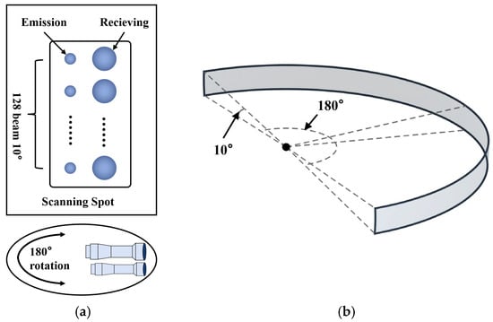
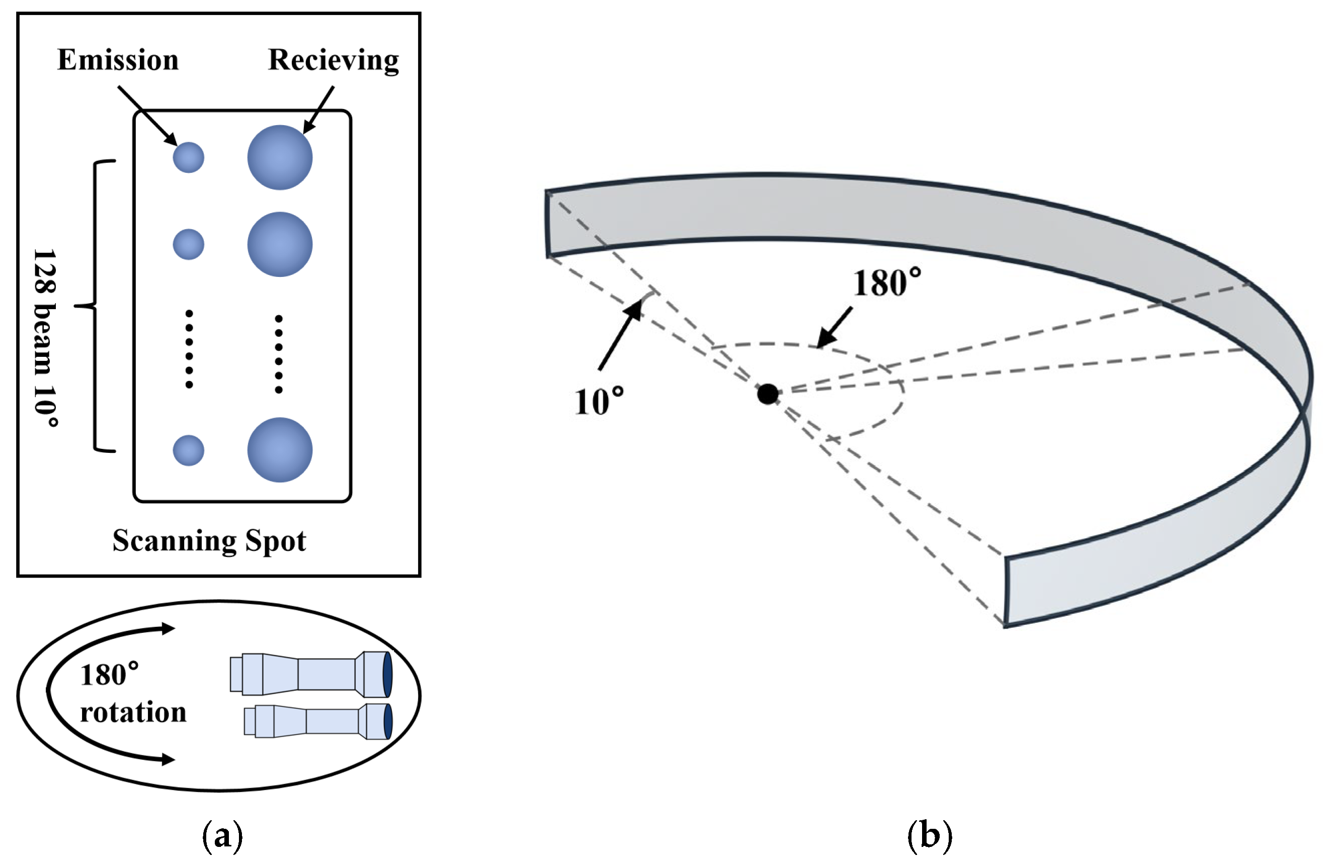
For port-environment perception, a 128-line scanning LiDAR constructed with single-photon avalanche diodes (SPADs) was employed [35]. In the vertical direction, 128 parallel transmit–receive channels are used to provide a 10° elevation field of view (FOV). In the horizontal direction, single-axis rotational scanning is implemented to provide a 180° azimuth FOV. To meet different requirements on azimuthal angular resolution, the scanning period can be set between one and three seconds; a longer period (lower rotational speed) yields higher azimuthal resolution and a denser laser point cloud. A schematic of the FOV is shown in Figure 1.

Figure 1. Schematic of the LiDAR scanning field of view. (a) Schematic of the scanning method. (b) Schematic of the field of view. The system provides an azimuth coverage of ±90° (180° total) and an elevation coverage of −6° to +4° (10° total).

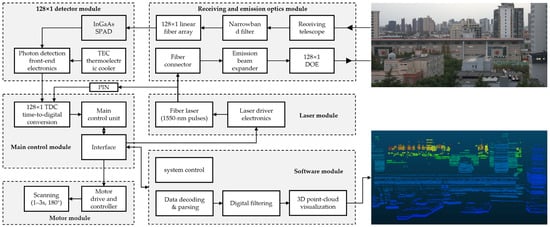
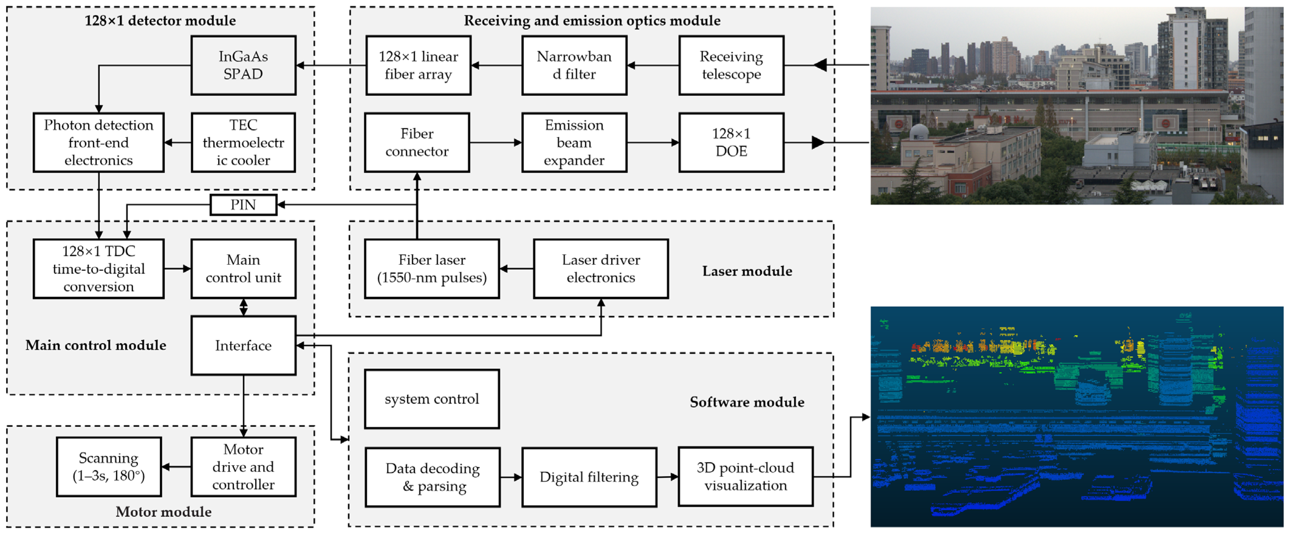
The panoramic-scanning single-photon-counting linear-array LiDAR comprises six modules: receiving and emission optics module, laser module, detector module, main control module, motor module, and software module. The system architecture and the principal parameters are shown in Figure 2 and Table 1.

Figure 2. LiDAR system framework.

Table 1. Key parameters of the lidar system.

Module	Parameters	Value
Laser	wavelength	1500 nm
	pulse energy per beam	0.78 μJ
	pulse repetition frequency (PRF)	20 kHz
Emission and receiving optics	divergence angle	0.15 mrad
	vertical angle resolution	1.37 mrad
	instantaneous field of view	0.3 mrad
	receiving optical aperture	34 mm
	photon detection efficiency (PDE)	>3%@1550 nm
Overall system	azimuth FOV	180°
	elevation FOV	10°
	scan period	1–3 s
	effective measurement range	50–3000 m
	range accuracy	0.09 m

The transmit–receive optics module includes the laser transmit optics, transmit beam-splitting optics, laser receive optics, linear-array receive fibers, and ultra-narrowband optical filtering. It is used for beam shaping and the emission of one hundred twenty-eight laser beams and for per-element alignment, filtering, and reception of the echo signals. The laser module comprises a high-repetition-rate fiber laser together with the laser driver and temperature-control electronics. A single-beam, high-repetition-rate, narrow-pulse 1550 nm laser output is generated and delivered via optical fiber to the optical path. The detector module consists of single-photon detectors and the associated quenching and shaping electronics. The one-hundred-twenty-eight fiber-coupled echo channels from the transmit–receive optics are detected on an element-by-element basis to produce photon-detection pulses, which are passed to the timing and angle-measurement electronics of the main control module. In this work, the single-photon detector is an InGaAs/InP Geiger-mode SPAD at 1550 nm developed by the Shanghai Institute of Technical Physics, Chinese Academy of Sciences. A single-photon detection efficiency of approximately three to eight percent at 1550 nm is provided. A three-stage thermoelectric cooler (TEC) is integrated, a TO-66 metal package is used, and fiber coupling is achieved via a fifty/one-hundred-micrometer multimode pigtail. The effective active-area diameter is thirty-five micrometers, meeting the requirements of this system for single-photon detection sensitivity and stability. Under the control of the drive electronics, the rotation module drives the above components through one hundred eighty degrees to realize one-dimensional panoramic scanning. The software module comprises data decoding and formatting, multithreaded point-cloud filtering, three-dimensional point-cloud visualization, and radar-system control. The control submodule governs system operation by issuing start and standby commands to the main control unit, as well as configuration commands such as scanning speed and left and right angular limits.

3. Methods

3.1. Data Characteristic Analysis

Within the high-rate ranging stream of a multi-echo, multi-line linear-array single-photon LiDAR, a single laser emission often produces multiple returns (caused by strong near-field reflections, semi-transparent media, or multipath), and the raw point cloud consequently contains numerous background photons induced by ambient illumination. Before applying any filtering, we analyze the following characteristics of the raw data:

• For an object of fixed physical size, its apparent angular span within the LiDAR field of view decreases with range; together with the LiDAR equation—which captures the decay of received power with distance and atmospheric attenuation—this reduces the usable point density and return energy at long ranges, making fixed-threshold filters prone to removing valid far-range points.
• For beam-steered scanners that employ a sinusoidally driven galvanometer, the angular velocity decreases near the scan edges, yielding higher sampling density at the edges.
• In multi-line systems, multiple vertical channels and fine elevation-angle resolutions imply that most macroscopic targets are not observed by a single line alone but instead form coherent tracks across adjacent lines.
• From a shape-prior perspective, most rigid targets manifest as continuous curves in the two-dimensional domain of pulse-time index versus range, whereas the background arising from atmospheric backscatter and dark counts is better modeled as a Poisson process. Accordingly, single-photon, multi-echo systems commonly employ time-windowed histogram statistics to suppress ambient background and dark counts.

Building on this analysis, we propose a histogram-based statistical filter with range adaptivity and adjacent-channel fusion (RA-ACF HSF). We first present the submethod, temporal–range histogram-based statistical filtering (TR HSF), detailing its principles and steps, and then, we introduce the improved RA-ACF HSF, together with its algorithmic rationale and procedure.

3.2. TR-HSF Algorithm

Given the raw ranging sequence

$$D={\left\{\left({\mathrm{\tau }}_j,r_j,c_j\right)\right\}}_{j=1}^N,{\mathrm{\tau }}_j\in Z, r_j\in R_{\ge 0}, c_j\in \{1,\dots ,C\}$$

(1)

where $D$ denotes the raw measurements, ${\tau }_j$ is the pulse-time index (the LiDAR pulse repetition frequency was set to 20 kHz. Assuming an acquisition duration of 1 s, the pulse-time index ${\tau }_j$ was taken to range from 1 to 20,000 and to denote the ${\tau }_j$-th laser emission, representing emission times as integers facilitates computation), $r_j$ is the range, and $c_j$ is the channel (beam) index. $C$ is the total number of channels, and $N$ is the total number of measurements. Let the within-frame multi-echo returns acquired by the channel $c$ at pulse time $t$ be the ascending set (stored in ascending order by range to support efficient interval counting):

$$S_{t,c}=\{ r_{t,c,1},\dots ,r_{t,c,n_{t,c}} \}$$

(2)

In the TR-HSF algorithm we process data for a single current channel $k$; for notational uniformity, we write ${\mathcal{C}}_{\mathcal{k}}=\left\{k\right\}$. For a candidate measurement $({\tau }_i,r_i,c_i)$ (with $c_i=k$ by default), TR-HSF first constructs a symmetric time window on the pulse axis with a half-width $W\in \mathbb{N}$:

$$T_i=\{ t\in Z\mid \left|t-{\tau }_i\right|\le W \},W\in N$$

(3)

On the range axis, it constructs a symmetric range interval defined by a radial-tolerance baseline $B_0>0$ and a relaxation factor $s\ge 0$:

$$I_i=\left[r_i-{\displaystyle \frac{{\Delta }_i}{2}}, r_i+{\displaystyle \frac{{\Delta }_i}{2}}\right],{\Delta }_i=s{B}_0$$

(4)

These define a local 2-D histogram neighborhood in the $(\tau ,r)$ plane centered at $({\tau }_i,r_i)$:

$$B_i=T_i\times I_i$$

(5)

For each $t\in T_i$, perform interval counting

$$c_{t,i}^{\left({\mathcal{C}}_{\mathcal{k}}\right)}=\sum _{c\in {\mathcal{C}}_{\mathcal{k}}}num\{ r\in S_{t,c}\mid r\in I_i \}=num\{ r\in S_{t,k}\mid r\in I_i \}$$

(6)

and accumulate over $T_i$ to obtain the histogram count (total votes):

$$v_i^{\left({\mathcal{C}}_{\mathcal{k}}\right)}=\sum _{t\in T_i}{c}_{t,i}^{\left({\mathcal{C}}_{\mathcal{k}}\right)}$$

(7)

Apply a binary decision with a minimum-occurrence threshold $M\in N$. Define

$${\mathrm{keep}}_{\mathrm{i}}=1\left(v_i^{\left({\mathcal{C}}_{\mathcal{k}}\right)}\ge \mathrm{M}\right)$$

(8)

and retain the measurement as a valid range if $v_i^{\left({\mathcal{C}}_{\mathcal{k}}\right)}\ge M$. The filtered output for the current channel $k$ is then

$$\widehat{D_k}=\{ \left({\tau }_i,r_i,c_i\right)\in D\mid c_i=k, {\mathrm{keep}}_{\mathrm{i}}=1 \},$$

(9)

The essence of TR-HSF is fixed-size histogramming within a local two-dimensional neighborhood in the pulse-time-index–range domain, suppressing isolated noise echoes and dark counts while reinforcing repeated near-neighbor observations of genuine targets as regular text.

3.3. RA-ACF HSF Algorithm

For the TR-HSF method, a fixed radial-tolerance baseline and a fixed minimum-occurrence threshold are not universally applicable across different range intervals. In far-range regions, the decline in usable point density and return energy makes valid measurements more likely to be removed by a fixed threshold; in near-range or locally high-density regions, a mismatch of filtering scale can lead to false retention. In addition, relying only on single-channel decisions tends to cause missed detections at channel boundaries and under occlusions due to insufficient statistical support. Simply broadening the filtering scale to restore structural connectivity may also introduce spurious connectivity and background noise. To address these issues, RA-ACF HSF extends TR-HSF with three improvements. First, it introduces a piecewise, range-adaptive parameter scheme: the radial-tolerance baseline and the minimum-occurrence threshold are adapted as a function of range while the short-term temporal window (half-width) is kept fixed. This yields more permissive scales and thresholds at long ranges and stricter ones at short ranges, mitigating far-range deletions and near-range false retention at the source. Second, it applies two-pass iterative refinement: An initial coarse pass with a slightly larger relaxation factor prioritizes the recovery of the connectivity of genuine curve or surface structures; a second pass then re-evaluates the first-pass output with a tightened relaxation factor to suppress spurious connectivity and boundary dilation. Third, it performs weakly coupled fusion of the immediately adjacent channels—one above and one below the current channel—by pooling their data with the current channel at the same filtering scale to compute a single weakly coupled histogram statistic. Neighboring-channel evidence compensates for insufficient support at occluded boundaries and for small far-range objects; from the fused result, only the measurements belonging to the current channel are retained as that channel’s final output. Overall, RA-ACF HSF incorporates range-aware and structure-aware cues into the statistical decision logic of TR-HSF, substantially reducing far-range deletions and boundary misses while improving the robustness and accuracy of the overall filtering.

The algorithmic workflow of RA-ACF HSF is presented below. To avoid repeating parts of the formulation, TR-HSF is first defined as a callable filtering operator, where $D_k$ denotes the pre-filtering data for a single channel; $W\in N,B_0>0,s>0,M\in N$ are fixed decision-scale parameters; and $\widehat{D_k}$ denotes the filtered output.

$$D_k=\{\left({\tau }_j,r_j,c_j\right)\in D\mid c_j=k\}$$

(10)

$$\widehat{D_k}=F_{TR-HSF}\left(D_k,W, B_0,s,M\right)$$

(11)

First, piecewise range adaptivity is applied to the radial-tolerance baseline $B_0$ and the minimum-occurrence threshold $M$, while the temporal-window half-width $W$ is kept constant:

$$B_0\left(r\right)=B_{0,l}, M\left(r\right)=M_l, r\in \left[r_{l-1},r_l\right)$$

(12)

$$r_{min}=r_0<r_1<\cdots <r_L=r_{max}$$

(13)

where $r$ is defined as the measured range, $r_{min}$ is defined as the lower bound of the valid detection interval, and $r_{max}$ is defined as its upper bound. To prevent the first filtering pass from being overly strict in scale, a global baseline for the minimum-occurrence threshold is introduced, and the smaller of this global threshold and the piecewise minimum-occurrence threshold is adopted.

$$M_g=\max \left(1, M_{\mathrm{global}}\right),\tilde{M}\left(r\right)=\min \{M\left(r\right), M_g\}$$

(14)

The TR-HSF algorithm with a larger relaxation factor $s_1$ is applied to complete the first pass of piecewise range-adaptive filtering at a relaxed scale.

$$\widehat{D_k^{\left(1\right)}}=F_{\mathrm{TR}-\mathrm{HSF}}\left(D_k; W,B_0\left(r\right),s_1,\tilde{M}\left(r\right)\right)$$

(15)

Based on the first-pass filtering result as input, a second filtering decision is performed with a smaller relaxation factor $s_2$.

$$s_2=\mathrm{\rho } s_1,0<\mathrm{\rho }<1$$

(16)

$$\widehat{D_k^{\left(2\right)}}=F_{\mathrm{TR}-\mathrm{HSF}}\left(\widehat{D_k^{\left(1\right)}}; W,B_0\left(r\right),s_2,\tilde{M}\left(r\right)\right)$$

(17)

To compensate for insufficient support in the number of signal points at object boundaries and for narrow far-range targets, a neighborhood dataset is constructed for the current channel $k$ by merging the range sequences of three channels to obtain $D_k^{\mathrm{fus}}$; this is not strictly limited to three channels, since, when beam data are sparse or some beams are inactive, five channels may be fused, whereas, when the detection density is higher, three or two channels may be fused for performance considerations.

$${\mathcal{C}}_{\mathcal{k}}=\{k-1, k, k+1\}\cap \{1,\dots ,C\}$$

(18)

$$D_k^{\mathrm{fus}}=\{\left({\mathrm{\tau }}_j,r_j,c_j\right)\in D\mid c_j\in {\mathcal{C}}_{\mathcal{k}}\}$$

(19)

The neighborhood data $D_k^{\mathrm{fus}}$ are subjected to two-pass piecewise range-adaptive filtering, yielding the filtering result for the three channels $\widehat{D_k^{\mathrm{fus}}}$:

$$\widehat{D_k^{\mathrm{fus}}}=F_{\mathrm{TR}-\mathrm{HSF}}\left(D_k^{\mathrm{fus}}; W,B_0\left(r\right),s_2,\tilde{M}\left(r\right)\right)$$

(20)

Finally, the range-sequence samples belonging to the current channel $k$ are selected as that channel’s filtered output $\widehat{D_k}$.

$$\widehat{D_k}=\{\left({\mathrm{\tau }}_i,r_i,c_i\right)\in \widehat{D_k^{\mathrm{fus}}}\mid c_i=k\}$$

(21)

To facilitate understanding of the execution procedure, the workflow of the RA-ACF HSF algorithm is provided below. Because presenting the complete algorithm in full detail would take substantial space, the implementation of TR-HSF has been open-sourced, and the code link is given in the Supplementary Materials. Therefore, TR-HSF is treated as a single step in the following workflow and is not elaborated in detail:

• Step 1. The range sequences $D={\{({\mathrm{\tau }}_j,r_j,c_j)\}}_{j=1}^N,{\mathrm{\tau }}_j\in Z, r_j\in R_{\ge 0}, c_j\in \{1,\dots ,C\}$ from all channels are taken as input.
• Step 2. The required hyperparameters are defined; examples of the piecewise parameter settings are provided in the open-source code, where all involved hyperparameters are also specified.
• Step 3. All channels are iterated over for processing; channel $k$ is used as an example.
• Step 4. Data from adjacent channels are acquired and merged to obtain $D_k^{\mathrm{fus}}=\{({\mathrm{\tau }}_j,r_j,c_j)\in D\mid c_j\in {\mathcal{C}}_{\mathcal{k}}\}$, which contains data from three channels.
• Step 5. A first-pass filtering is applied to $D_k^{\mathrm{fus}}$, yielding

  $$\widehat{D_k^{\mathrm{fus}\left(1\right)}}=F_{\mathrm{TR}-\mathrm{HSF}}\left(D_k^{\mathrm{fus}}; W,B_0\left(r\right),s_1,\tilde{M}\left(r\right)\right)$$
• Step 6. A second-pass filtering is applied to $\widehat{D_k^{\mathrm{fus}\left(1\right)}}$,yielding

  $$\widehat{D_k^{\mathrm{fus}\left(2\right)}}=F_{\mathrm{TR}-\mathrm{HSF}}\left(D_k^{\mathrm{fus}}; W,B_0\left(r\right),s_2,\tilde{M}\left(r\right)\right)$$
• Step 7. From $\widehat{D_k^{\mathrm{fus}\left(2\right)}}$, only the range-sequence samples belonging to $D_k=\{\left({\tau }_j,r_j,c_j\right)\in D\mid c_j=k\}$ are selected as the filtered result for the current channel $k$.

3.4. Numerical Simulation

To evaluate the denoising performance of different point-cloud filtering algorithms, the filter outputs are partitioned into four categories: true positives (TP), in which genuine signals are correctly retained; true negatives (TN), in which noise is correctly removed; false positives (FP), in which noise is misclassified as signal; and false negatives (FN), in which genuine signals are missed. On this basis, three commonly used metrics are employed. Precision (P) describes the proportion of samples labeled as signals that are in fact genuine signals and is therefore related to false positives. Recall (R) describes the proportion of genuine signals that are successfully detected and are sensitive to false negatives. Because precision and recall often trade off with threshold settings, the F1 score (F1)—the harmonic mean of P and R—is adopted as an overall measure of filtering performance; a higher value indicates better post-filtering discrimination quality. The corresponding formulas are as follows:

$$\mathrm{P}={\displaystyle \frac{\mathrm{T}\mathrm{P}}{\mathrm{T}\mathrm{P}+\mathrm{F}\mathrm{P}}}$$

(22)

$$\mathrm{R}={\displaystyle \frac{\mathrm{T}\mathrm{P}}{\mathrm{T}\mathrm{P}+\mathrm{F}\mathrm{N}}}$$

(23)

$$\mathrm{F}1={\displaystyle \frac{2\mathrm{P}\mathrm{R}}{\mathrm{P}+\mathrm{R}}}$$

(24)

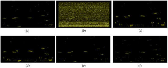
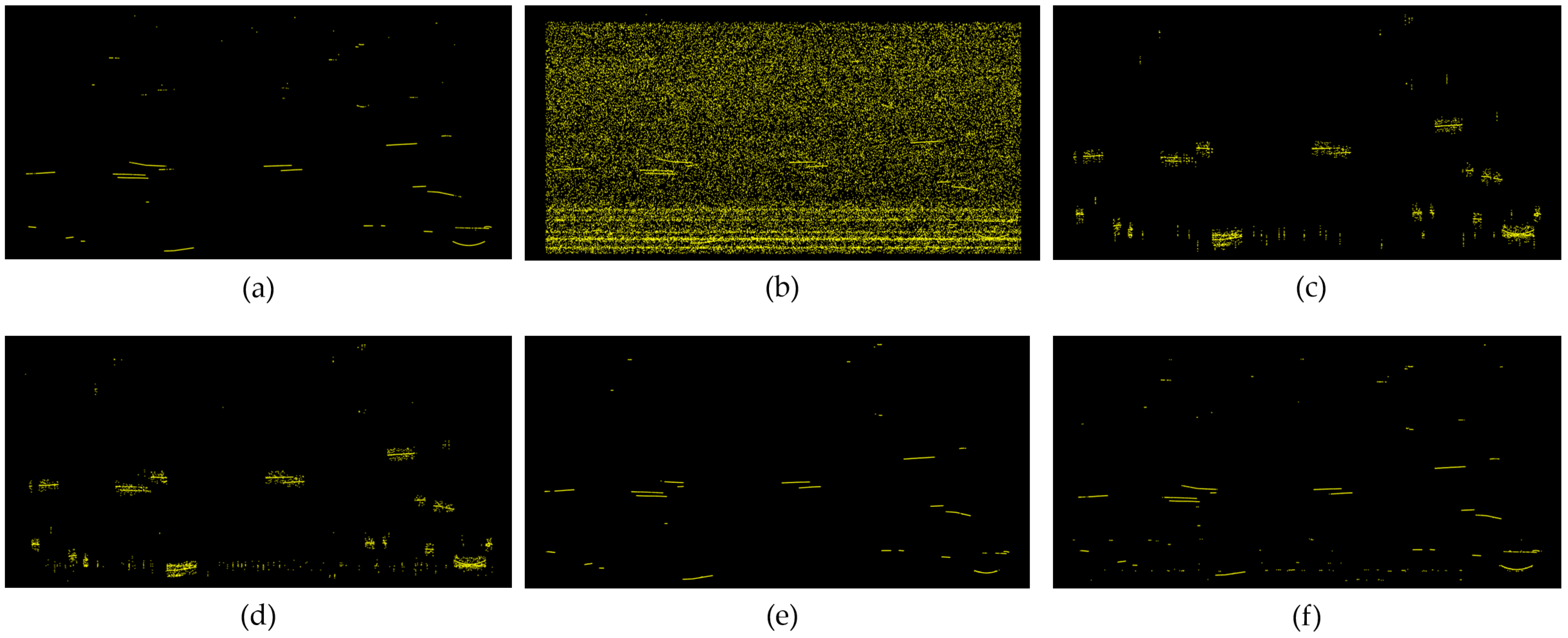
Here, synthetic simulation data were constructed on the basis of raw LiDAR data from a single channel, and a unified simulation–validation workflow was established for generation, denoising, and metric-based comparison. First, the noise intensity and its range dependence were parametrically estimated from real data. A single ground-truth trajectory was then generated within one frame to cover multi-scale scenarios—near, mid, far, and fine long-range segments—using geometric curves including line segments, circular arcs, sinusoids, and polylines; time jitter and offsets were injected to reflect timing and ranging errors. Poisson-distributed noise points were superimposed on the ground truth according to a target noise-to-inlier ratio so as to achieve a prescribed ratio of noise to signal points. In the evaluation stage, the filtering results of RA-ACF HSF (without adjacent-channel fusion) were compared with those of DBSCAN, ROR, and TR-HSF under a noise-to-inlier ratio of ten, and the metrics TP, FP, FN, recall R, precision P, and F1 score F were tallied. The filtering outcomes at a noise-to-inlier ratio of ten are shown in Figure 3, and the specific metrics are listed in Table 2, where the denoising effectiveness of RA-ACF HSF was superior to that of the other algorithms.

Figure 3. Comparison of filtering results on simulated data: (a) ground-truth signal points, (b) after noise injection, (c) DBSCAN, (d) ROR, (e) TR-HSF, and (f) RA-ACF HSF.

Table 2. Performance of different denoising algorithms.

Algorithm	Evaluation Metrics
	TP	FP	FN	P	R	F1
DBSCAN	4211	2503	1142	0.6271	0.7866	0.6979
ROR	4682	2449	671	0.6565	0.8746	0.7500
TR-HSF	4887	642	466	0.8838	0.9129	0.8981
RA-ACF HSF	5271	972	82	0.8443	0.9846	0.9091

3.5. Sensitivity Analysis and Ablation Study

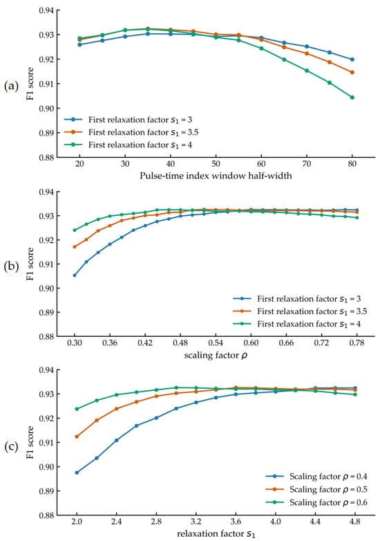
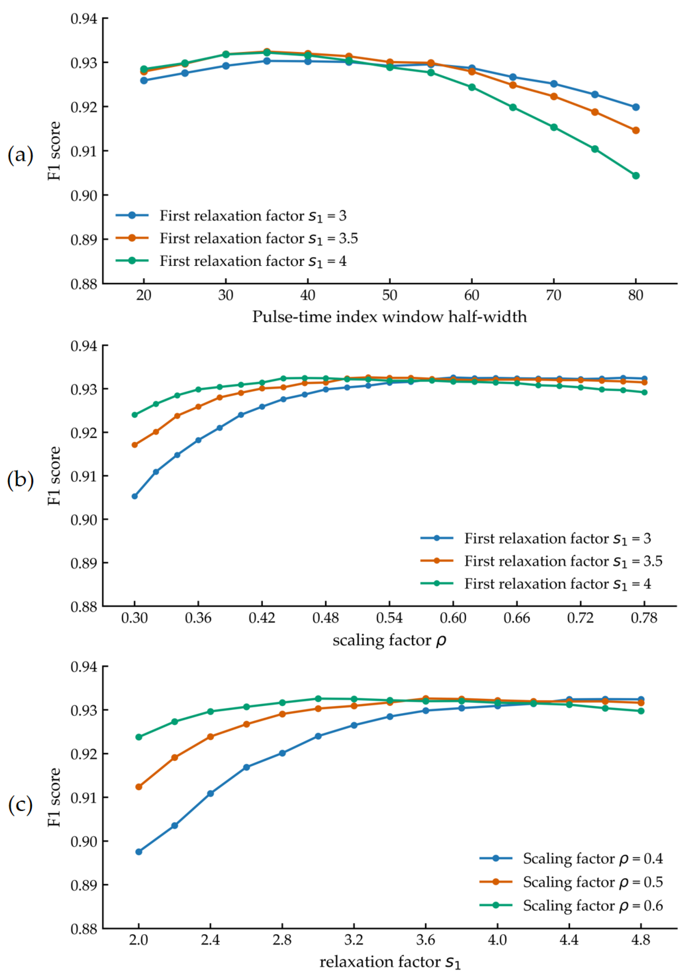
To assess the sensitivity of the proposed RA-ACF HSF method to the key hyperparameters—half-width $W$, relaxation factor $s$, and scaling factor $\rho$—and to quantify the benefit brought by the two-pass iterative strategy, the following experiments were designed and implemented. A comprehensive evaluation was conducted using the F1 score. To provide an intuitive view of parameter sensitivity, the y-axis range of all figures in this section was fixed to 0.88–0.94; the amplitude of curve fluctuations is taken to indicate the degree of sensitivity.

With all other parameters held constant, the half-width $W$ (of the temporal window) was swept from 20 to 80 in increments of 5, and the F1 score was computed for each setting. Three experimental groups with different relaxation factors $s$ were configured, as shown in Figure 4a. It was observed that RA-ACF HSF is sensitive to $W$ and that choosing a $W$ value that is either too large or too small leads to a decrease in the F1 score.

Figure 4. Hyperparameter sensitivity analysis of the algorithm: (a) half-width $W$; (b) scaling factor $\rho$; (c) relaxation factor $s$.

For the scaling factor $\mathrm{\rho }$, experiments were conducted from 0.3 to 0.8 in increments of 0.02. Given the strong correlation between $\mathrm{\rho }$ and the initial relaxation factor ${\mathrm{s}}_1$, three values of ${\mathrm{s}}_1$ (3, 3.5, and 4) were selected to enhance persuasiveness, and the F1 score was computed for each setting, as shown in Figure 4b. It was observed that, although the optimal value of $\mathrm{\rho }$ may differ across ${\mathrm{s}}_1$, the F1 score at the optimum is nearly identical. Similarly, a sensitivity analysis was performed for the initial relaxation factor ${\mathrm{s}}_1$, sweeping from 2 to 5 in increments of 0.2 (cases with ${\mathrm{s}}_1$ in the range 1–2 yielded very low F1 scores and were therefore not included). Three different scaling factors (0.4, 0.5, and 0.6) were chosen, and the F1 score was recorded for each setting, as shown in Figure 4c. The optimal ${\mathrm{s}}_1$ was found to decrease as the scaling factor increased, while the F1 score at the optimum exhibited only minor variations.

To quantify the algorithm-level benefit of the two-pass iterative strategy, experiments were conducted with the half-width $W$ fixed at 35, the first relaxation factor $s_1$ fixed at 3.5, and all other parameters held constant. The scaling factor $\rho$ was set to 0.4, 0.5, and 0.6 in three groups, and the F1 score was computed in each case, as shown in Table 3. For the single-pass RA-ACF HSF ablation, the relaxation factor was set either to $s_1$ or $s_2=\rho s_1$. The ablation results indicate that, although the overall improvement in F1 achieved by introducing the two-pass strategy is modest, consistent positive gains were observed across different test conditions.

Table 3. Performance of RA-ACF HSF (2 pass) and RA-ACF HSF (1 pass only).

Algorithm	Evaluation Metrics
	TP	FP	FN	P	R	F1
RA-ACF HSF (3.5)	5287	947	66	0.8480	0.9876	0.9125
RA-ACF HSF (1.4)	5210	656	143	0.8881	0.9732	0.9287
RA-ACF HSF (3.5–1.4)	5207	649	146	0.8891	0.9727	0.9290
RA-ACF HSF (3.5)	5287	947	66	0.8480	0.9876	0.9125
RA-ACF HSF (1.75)	5258	677	95	0.8859	0.9822	0.9316
RA-ACF HSF (3.5–1.75)	5256	665	97	0.8876	0.9818	0.9324
RA-ACF HSF (3.5)	5287	947	66	0.8480	0.9876	0.9125
RA-ACF HSF (2.1)	5269	700	84	0.8827	0.9843	0.9307
RA-ACF HSF (3.5–2.1)	5267	681	86	0.8855	0.9839	0.9321

4. Experiment and Results Analysis

4.1. Experimental Setup

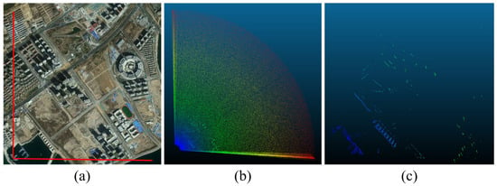
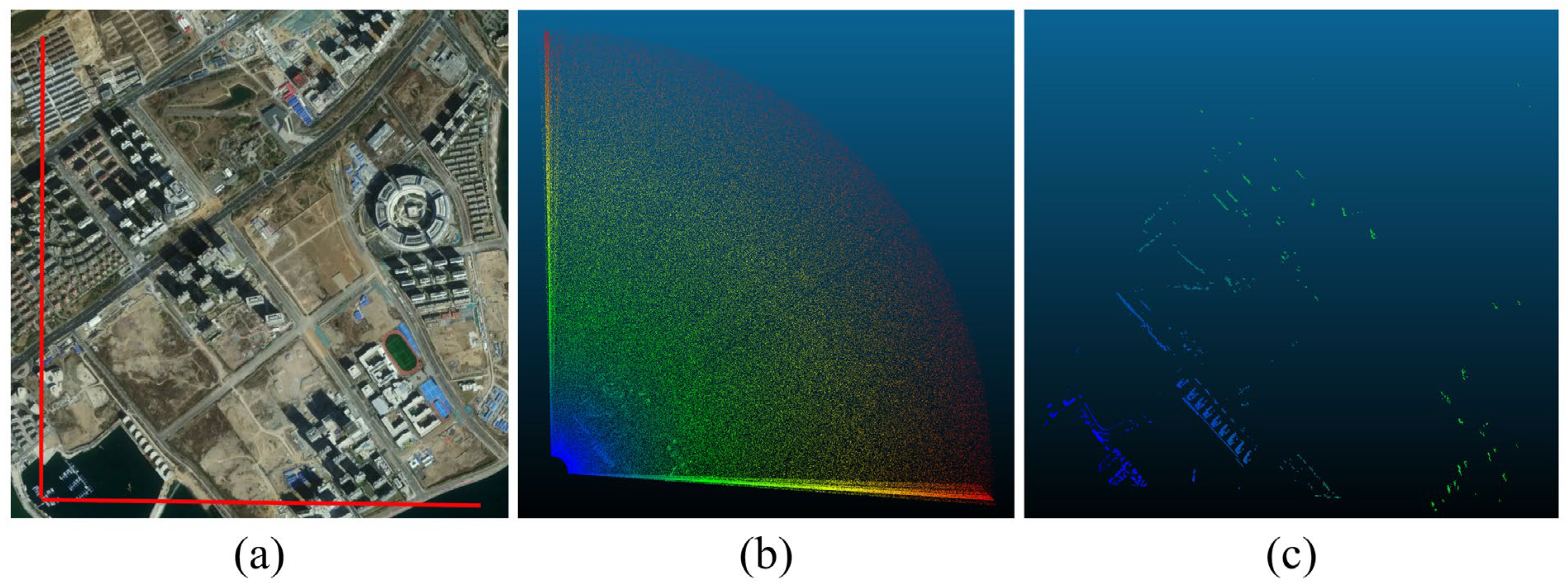
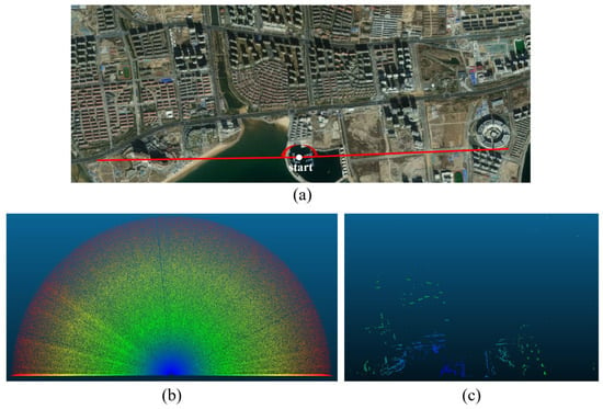
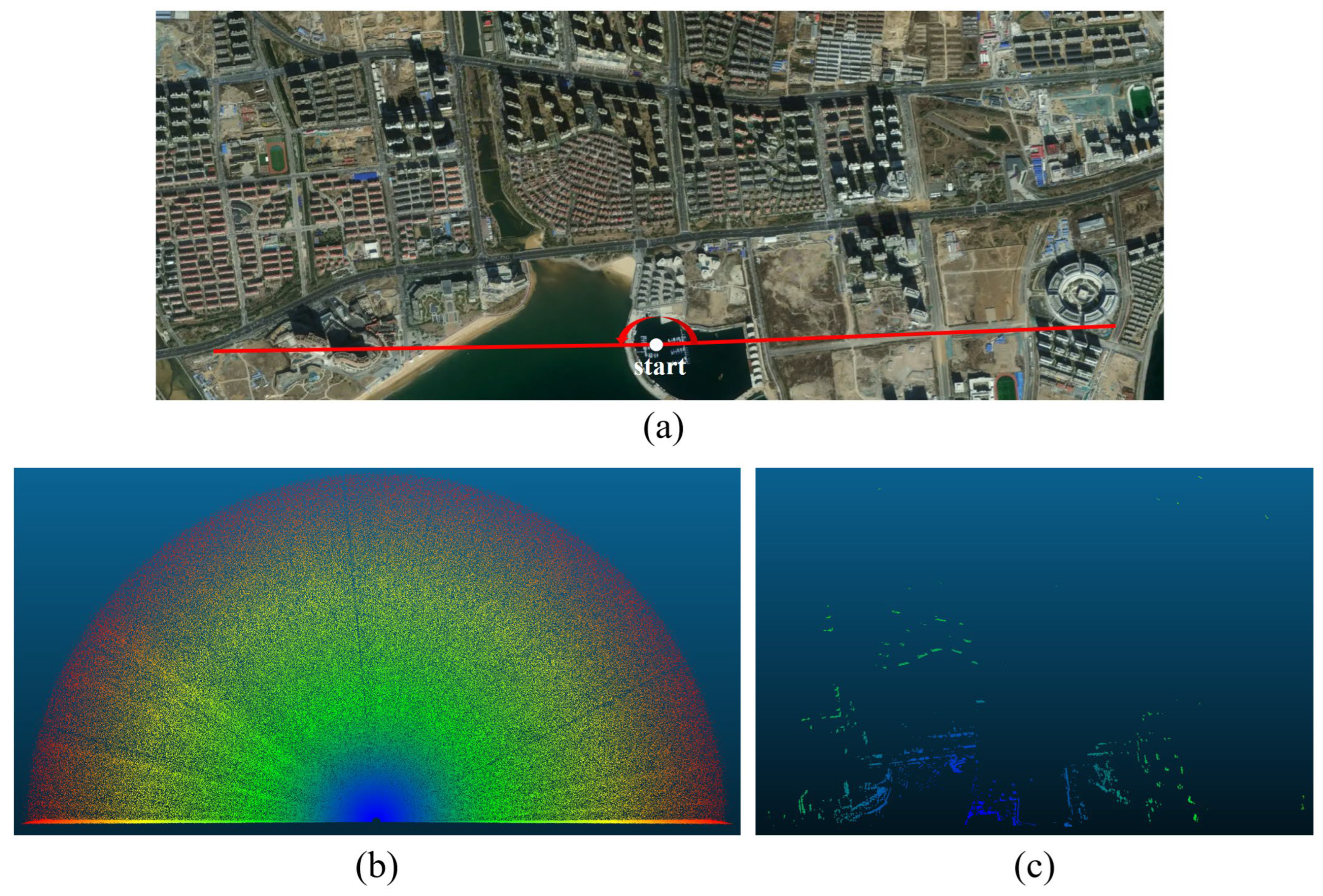
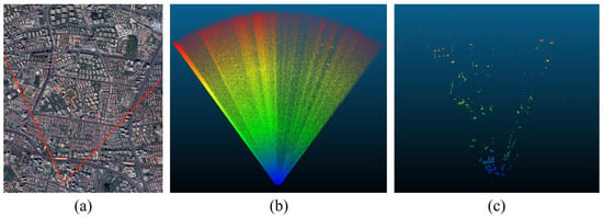
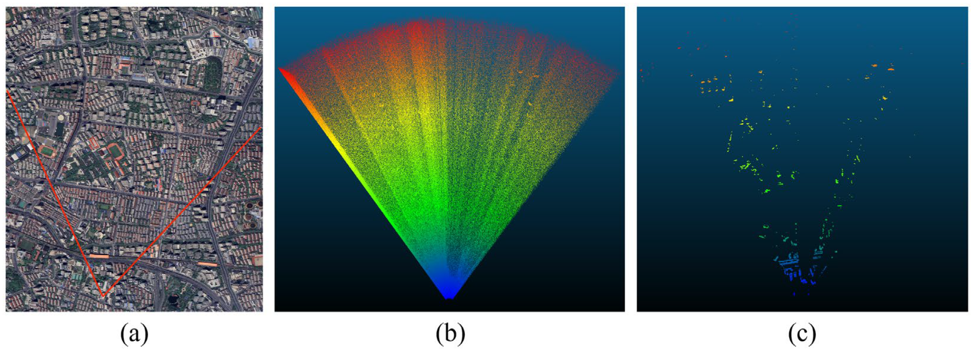
In this study, the panoramic-scanning single-photon-counting linear-array LiDAR designed in Section 2 was installed on a vessel in the port area and on a rooftop in the urban area, and environmental-perception experiments were conducted on the waterside and the landside to verify the capability of the system and the algorithm to perceive targets in different scenarios. Multiple experiments were performed under different scenarios, raw data were collected for each scenario, and the acquired raw point-cloud data were filtered with the RA-ACF HSF algorithm proposed herein. First, experimental data acquisition was carried out at a port near Lingshan Bay in Qingdao, Shandong province; the LiDAR device was mounted on a vessel operating near the port, and two datasets in different viewing directions were collected, as shown in Figure 5 and Figure 6. Figure 5a and Figure 6a present satellite maps of the areas scanned by the LiDAR in the test scenes; Figure 5b and Figure 6b show the imaging results of the point clouds before filtering; Figure 5c and Figure 6c show the imaging results of the point clouds after filtering. Thereafter, the experimental apparatus was installed on a high-rise building near Chifeng Road metro station in Shanghai; one dataset was acquired, and filtering was performed, as shown in Figure 7.

Figure 5. Qingdao, 90° field of view, and LiDAR sensing post-filtering results: (a) satellite image; (b) LiDAR point-cloud image before filtering (point count: 345,089); (c) LiDAR point-cloud image after filtering (point count: 34,957).

Figure 6. Qingdao, 180° field of view, and LiDAR sensing post-filtering results: (a) satellite image; (b) LiDAR point-cloud image before filtering (point count: 983,421); (c) LiDAR point-cloud image after filtering (point count: 105,564).

Figure 7. Shanghai, 70° field of view, and LiDAR sensing post-filtering results: (a) satellite image; (b) LiDAR point-cloud image before filtering (point count: 12,83,882); (c) LiDAR point-cloud image after filtering (point count: 331,137).

4.2. Results and Analysis

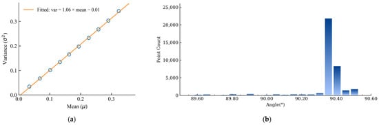
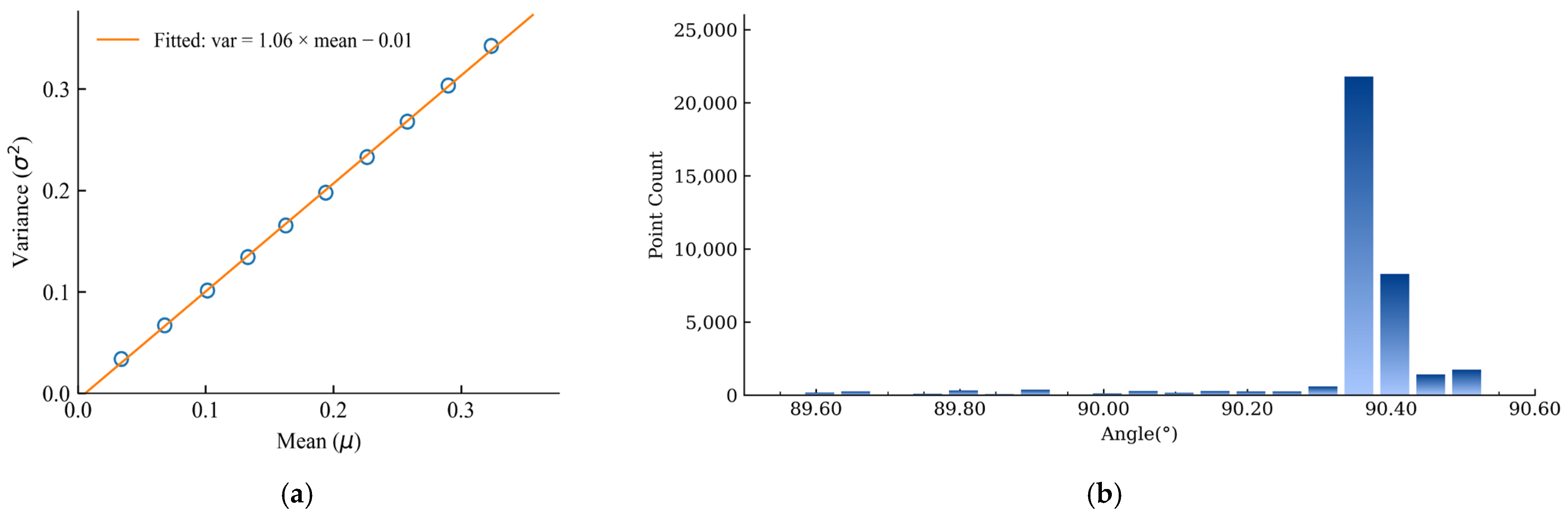
Owing to differences in range and reflectivity among objects within the scan field, the spatial locations and detection probabilities of target points vary, which increases randomness and hampers direct analysis. Therefore, in single-photon LiDAR data, analyses of the noise distribution are performed more frequently. A segment acquired over an open area was selected, and data beyond one thousand meters were extracted for noise-distribution analysis (only several sky-pointing beams were used). Successive three-hundred-meter range intervals were formed; for each interval, the mean and variance of the noise counts were computed, and a linear fit was performed, as shown in Figure 8a. The fitted line has a slope of 1.07 and an intercept of −0.01, which is, from an engineering standpoint, fully consistent with a Poisson distribution, indicating that the addition of Poisson-distributed noise in simulation is reasonable.

Figure 8. Point-cloud feature analysis: (a) variance vs. mean of noise counts and linear fit; (b) point-cloud density distribution at the scan boundary.

The point-cloud count at a boundary in Figure 6b was tallied. A one-degree angular sector at the boundary was selected. To reduce the influence of near-range targets, only points with ranges greater than 2000 m were included (the maximum detection range of this dataset is 4000 m). The number of raw point-cloud samples within successive 0.05-degree angular intervals was then computed, as shown in Figure 8b. A pronounced surge in point count was observed at the boundary, which is attributed to a brief pause of the rotary drive motor during the turnaround of the reciprocating scan; this observation is consistent with the prior analysis that point-cloud density increases at scan edges. The angle bin with the largest point count was not located at the maximum angle. During acceleration and deceleration in the reversal, due to limited servo bandwidth, the actual position lags the command during acceleration/deceleration, causing the zero-velocity turnaround to occur inside the commanded angular limit [36].

Considering deployment on resource-limited platforms, a brief analysis of computational cost was deemed necessary. Using the Shanghai dataset as an example, the acquisition lasted approximately 1.8 s and contained about 1.3 million points. Algorithm memory usage (AMU) was defined as AMU = PEAK_end − RSS_start, where RSS denotes the resident set size (RAM currently in use) and PEAK denotes the peak RAM usage observed during execution. Runtime memory consumption for each algorithm was recorded and analyzed, as shown in Table 4. It was observed that the implemented TR-HSF and RA-ACF HSF maintained small runtime footprints: Memory usage remained below 500 MB throughout execution, indicating that deployment is feasible even on platforms with 512 MB of RAM and providing a clear advantage in memory usage. On an Intel Core i5 CPU with multithreading enabled, a filtering time of about 1.4 s was measured for TR-HSF, which is shorter than the acquisition time and thus satisfies real-time requirements; however, after introducing range adaptivity and adjacent-channel fusion, the real-time performance of RA-ACF HSF has not yet fully met expectations.

Table 4. Memory usage comparison of different algorithms.

Algorithm	Start RSS	Start PEAK	End PEAK	End PEAK	AMU	Average AMU
DBSACN	428.7	428.7	1488.1	1488.1	1059.4	1001.8333
	409.3	409.3	1345.7	1345.7	936.4
	363.7	363.7	1373.4	1373.4	1009.7
ROR	436.9	436.9	756.2	756.2	319.3	407.2666
	417.5	417.5	904.8	904.8	487.3
	362.1	362.1	777.3	777.3	415.2
TR-HSF	372.7	372.7	391.1	391.1	18.4	18.3666
	414.6	414.6	431.1	431.1	16.5
	433.8	433.8	454.0	454.0	20.2
RA-ACF HSF	383.5	383.5	317.6	411.8	28.3	21.9
	380.8	380.8	297.3	400.1	19.3
	380.1	380.1	398.2	411.3	18.1

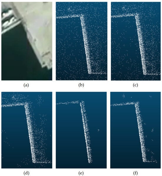
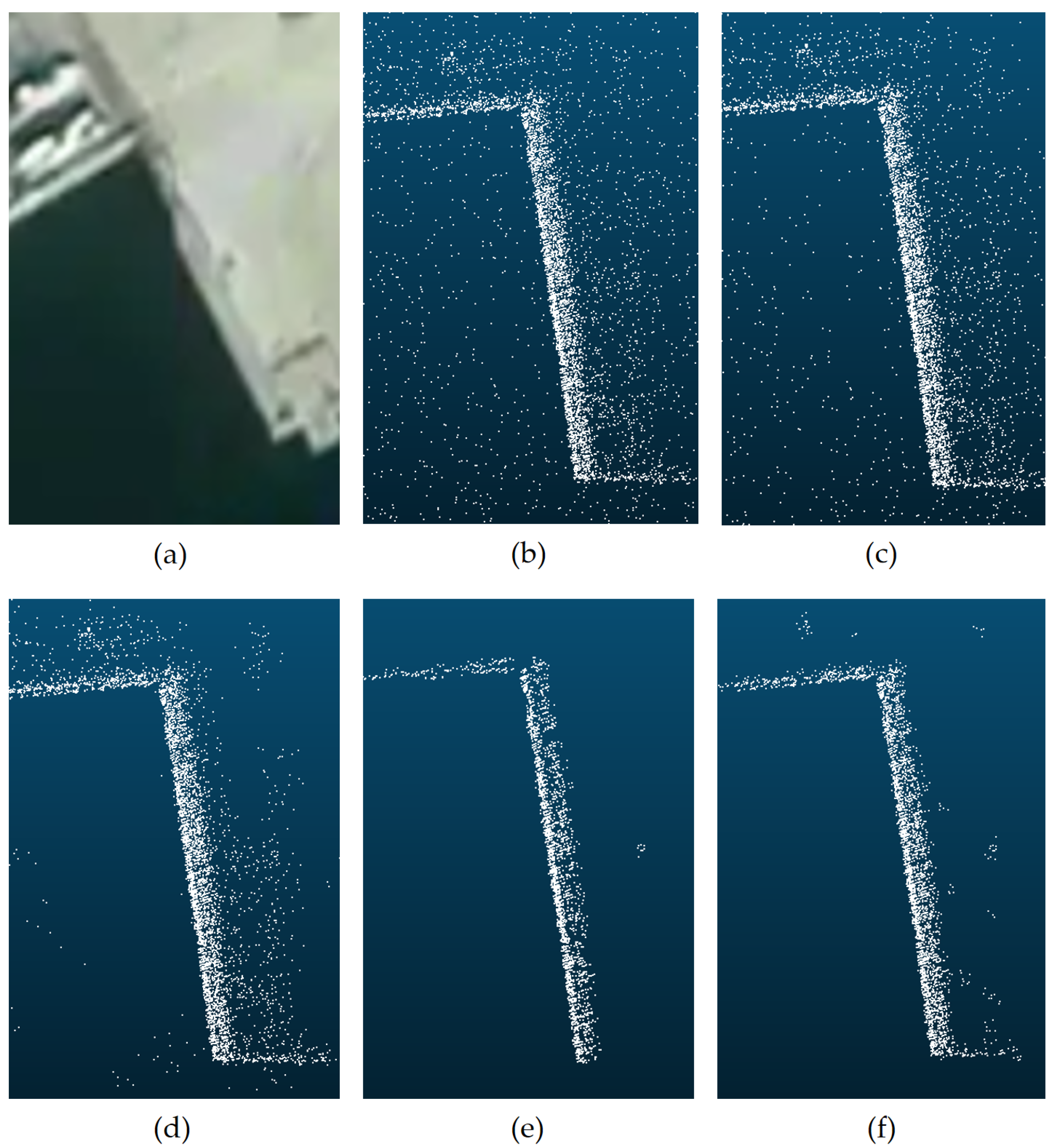
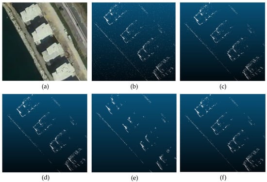
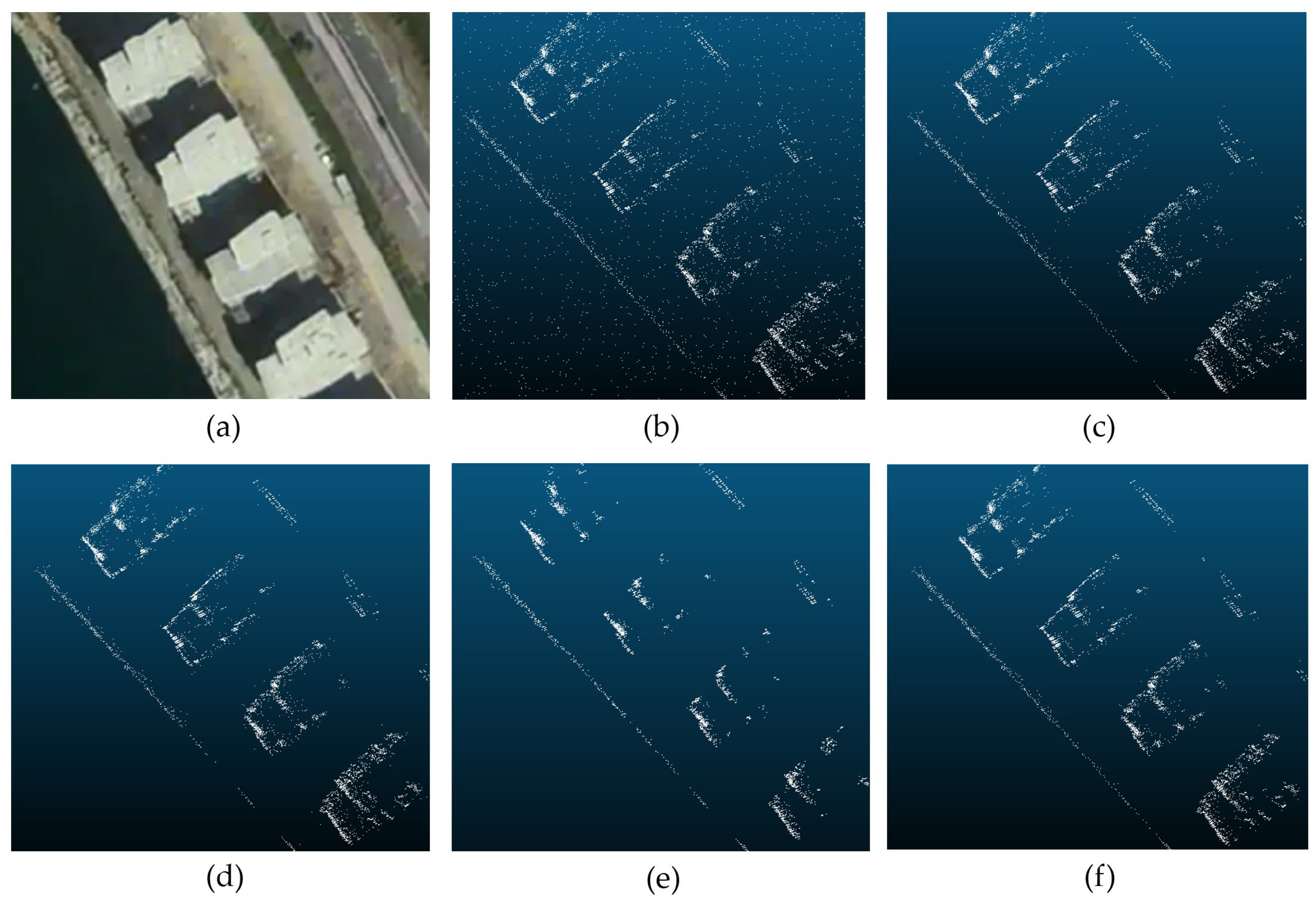
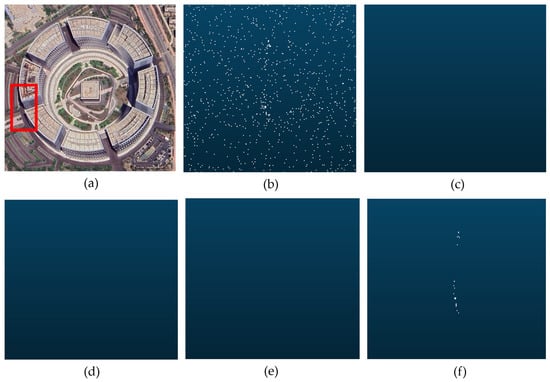
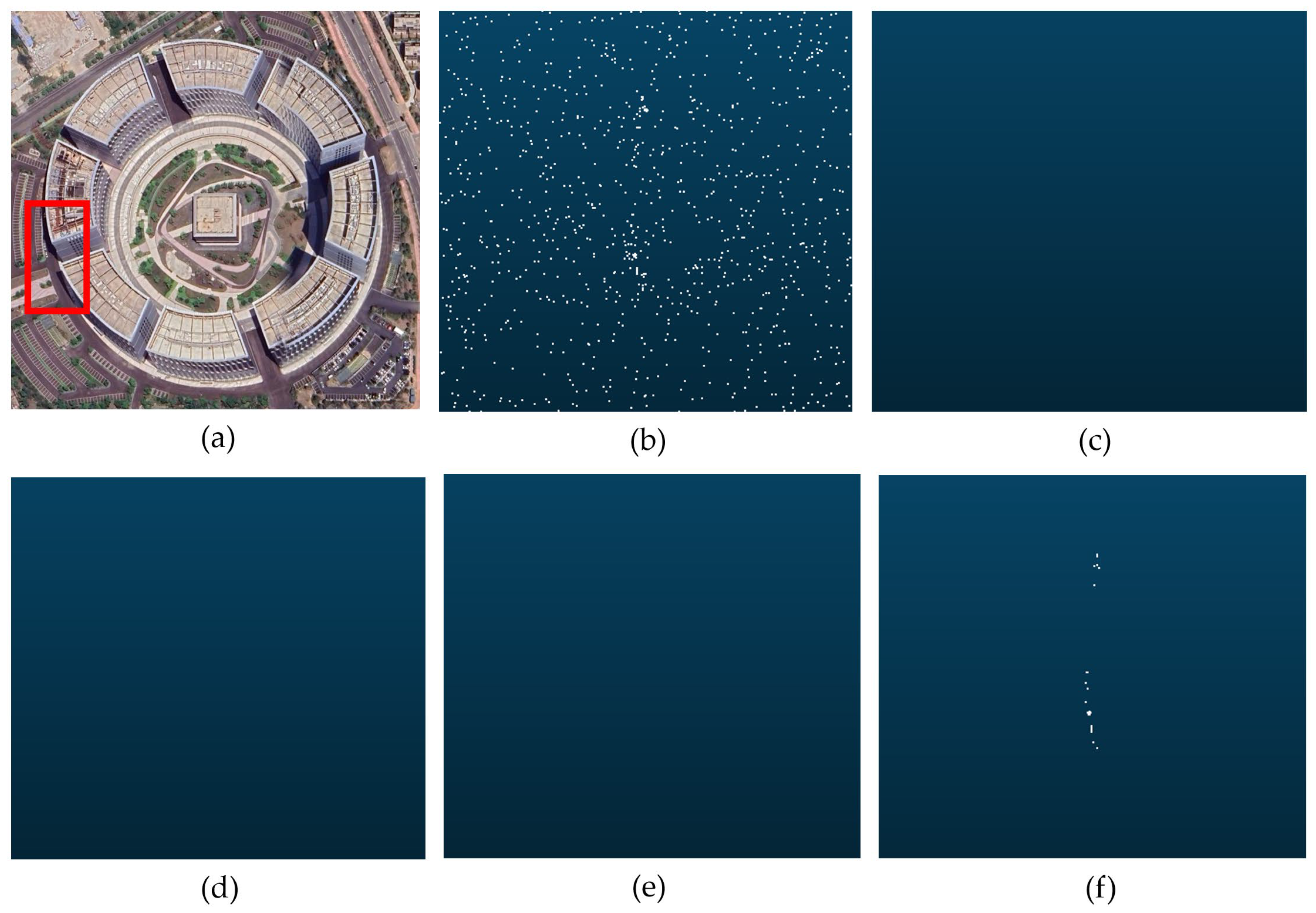
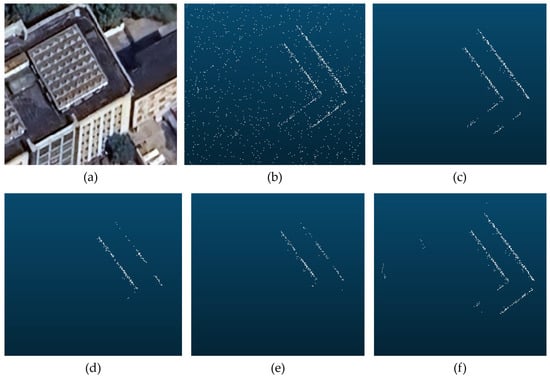
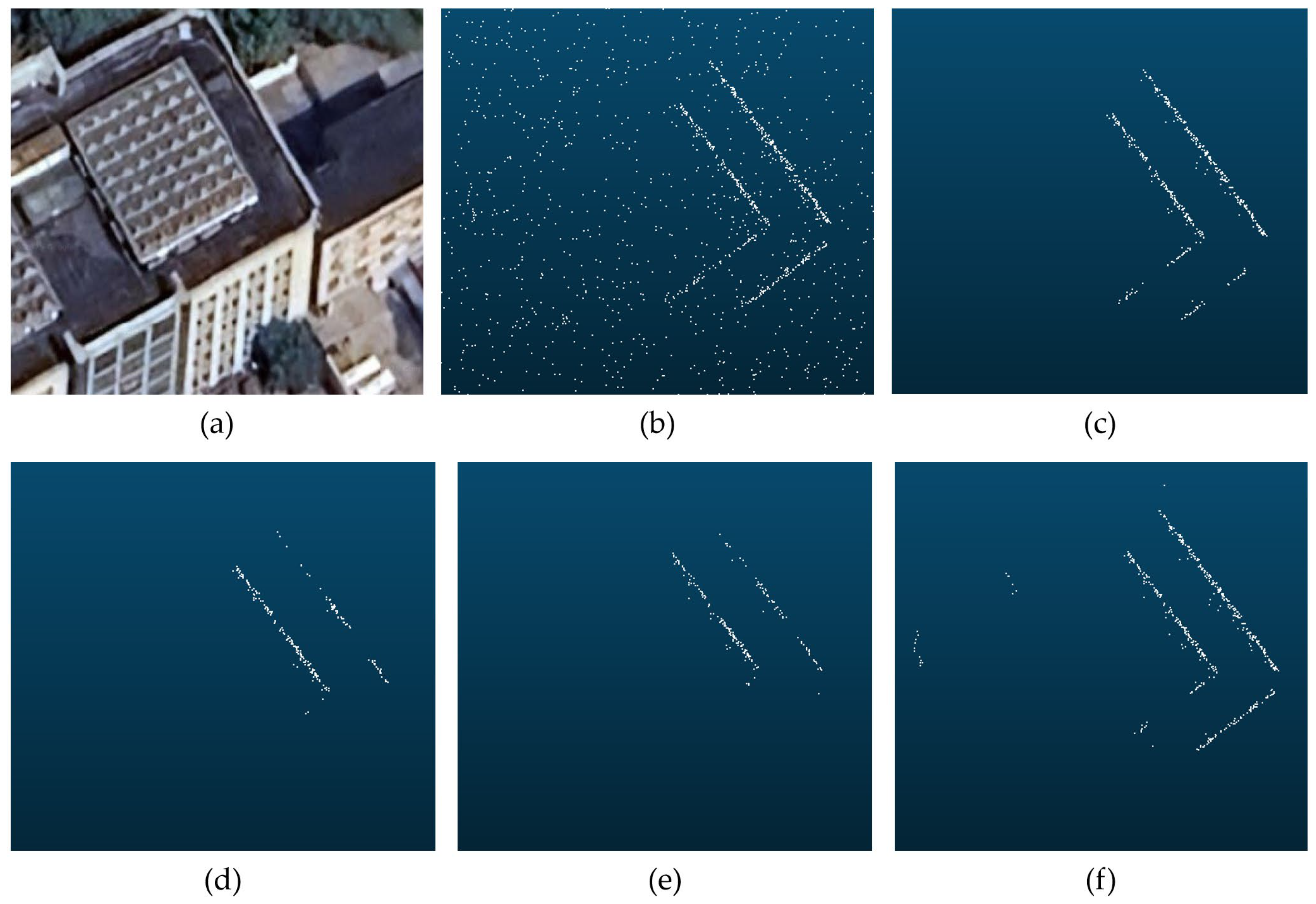
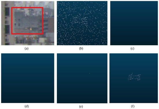
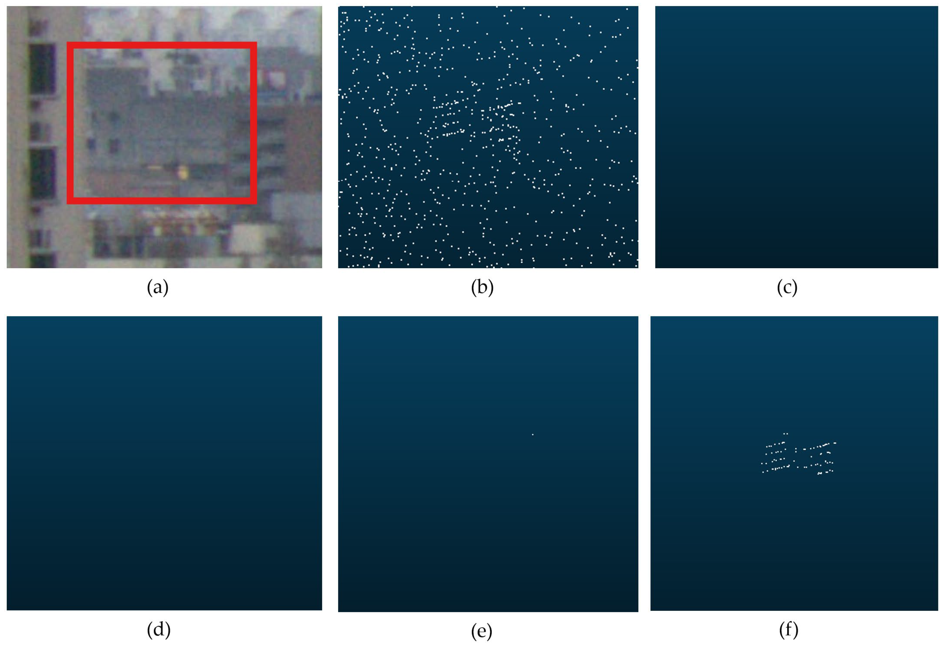
Imaging of the shoreline at 120 m, the shoreline and buildings at 500 m, and a circular building at 1800 m was performed for the harbor dataset, and the results of several filtering methods were compared, as shown in Figure 9, Figure 10 and Figure 11. It was observed that DBSCAN exhibited substantial noise in the near-range interval; noise decreased to some extent in the mid-range interval, but small targets at far range were not effectively preserved. ROR showed considerable noise in the near-range interval; although noise was effectively reduced in the mid-range interval, structural preservation was locally incomplete, a small discontinuity appeared on the shoreline in Figure 9d, and small far-range targets were not effectively preserved. TR-HSF (with a filtering scale selected for the near-range interval) achieved the best near-range filtering, but many instances of incomplete structural preservation occurred in the mid-range interval, and small far-range targets were not fully retained. By contrast, the proposed RA-ACF HSF achieved strong noise suppression and structural preservation in all three scenarios.

Figure 9. Comparison of denoising results for different algorithms for the shoreline at 90 m: (a) satellite image; (b) point cloud before denoising (point count: 5507); (c) DBSCAN (point count: 5326); (d) ROR (point count: 4835); (e) TR-HSF (point count: 2674); (f) RA-ACF HSF (point count: 3564).

Figure 10. Comparison of denoising results for different algorithms for the shoreline and buildings at 500 m: (a) satellite image; (b) point cloud before denoising (point count: 7472); (c) DBSCAN (point count: 6254); (d) ROR (point count: 5986); (e) TR-HSF (point count: 3447); (f) RA-ACF HSF (point count: 5628).

Figure 11. Comparison of denoising results for different algorithms for the circular building at 1800 m: (a) satellite image; (b) point cloud before denoising (point count: 717); (c) DBSCAN (point count: 0); (d) ROR (point count: 0); (e) TR-HSF (point count: 0); (f) RA-ACF HSF (point count: 25).

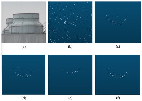
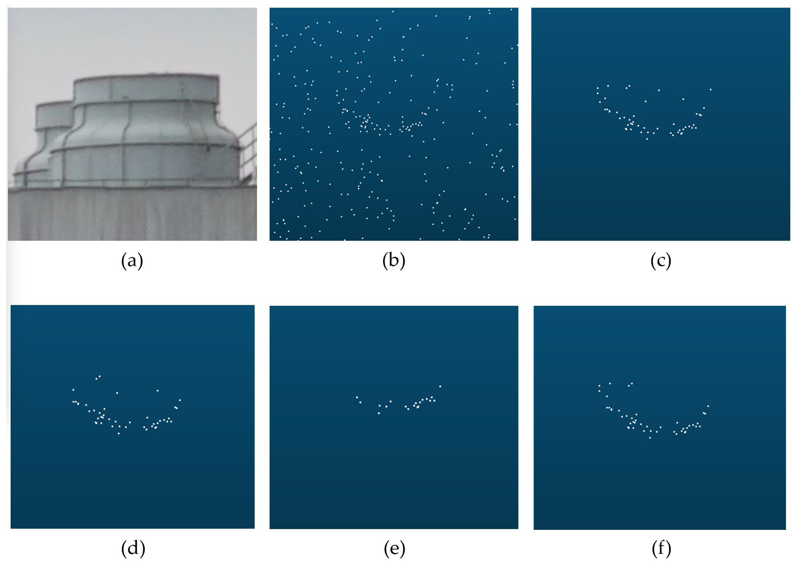
The RA-ACF HSF algorithm was found to provide good filtering capability for small objects, building outlines, and distant tall building facades. From the urban dataset, a cylindrical exhaust vent at 280 m, a building corner and rooftop fine structures at 1100 m, and a building at 2400 m were selected for comparison across different filtering algorithms (Figure 12, Figure 13 and Figure 14). Among these, only RA-ACF HSF effectively preserved the side surfaces of the small rooftop columns detected at 1100 m and the building facade at 2400 m that was partially occluded by other buildings, demonstrating that weak signals can be extracted under high-noise backgrounds while strong noise suppression is maintained.

Figure 12. Comparison of denoising results for different algorithms for the cylindrical rooftop vent at 280 m: (a) satellite image; (b) point cloud before denoising (point count: 96); (c) DBSCAN (point count: 65); (d) ROR (point count: 45); (e) TR-HSF (point count: 20); (f) RA-ACF HSF (point count: 56).

Figure 13. Comparison of denoising results for different algorithms for the building-corner outline at 1100 m: (a) satellite image; (b) point cloud before denoising (point count: 1237); (c) DBSCAN (point count: 414); (d) ROR (point count: 206); (e) TR-HSF (point count: 186); (f) RA-ACF HSF (point count: 454).

Figure 14. Comparison of denoising results for different algorithms for the building facade at 2400 m: (a) satellite image; (b) point cloud before denoising (point count: 1084); (c) DBSCAN (point count: 0); (d) ROR (point count: 0); (e) TR-HSF (point count: 1); (f) RA-ACF HSF (point count: 88).

Based on the port and urban experimental scenarios and through comparative analyses of the filtering results for multiple targets at different ranges and with different structures, the RA-ACF HSF algorithm was shown to suppress noise effectively for targets across all range intervals and to preserve weak long-range signals, thereby demonstrating excellent filtering capability in point-cloud processing.

5. Conclusions

In this study, a multi-line linear-array single-photon LiDAR system supporting wide-area, long-range sensing was designed and implemented, and a novel point-cloud filtering algorithm was proposed, by which the high-quality detection and extraction of targets at different ranges were achieved. Based on an analysis of the characteristics of raw LiDAR signals and noise, a point-cloud filtering method suitable for a large ranging span and high beam density was developed. A distance-adaptive parameterization mechanism was introduced, and adjacent-channel data were fused to provide statistical support; compared with unoptimized DBSCAN, ROR, and TR-HSF, the filtering capability was significantly improved, with better preservation of weak long-range returns. It was experimentally verified that targets at 2400 m could be effectively extracted by the system, even when the post-filtering signal-point density was relatively sparse. Robust technical support and a practical reference for future engineering applications in intelligent shipping, autonomous navigation and berthing, target tracking, maritime collision warning, and the construction of digital-twin ports are provided by the proposed single-photon LiDAR system and point-cloud filtering algorithm.

Although the LiDAR system and the proposed algorithm demonstrate substantial application value for three-dimensional environmental perception, several limitations remain. The Poisson noise model adopted during simulation still deviates from the noise statistics observed in real scenes. While TR-HSF can be executed in real time, the present implementation of RA-ACF HSF does not yet fully meet real-time requirements. Future work will focus on further calibrating and refining the noise model using richer field datasets. In addition, learning-based methods will be explored by combining GAN-based super-resolution generation for sparse data [37] with Transformer-based spatiotemporal dependency modeling [38], with the aim of building a system that enhances training under extreme scenarios and supports ICTA’s high-resolution reconstruction and prediction of future distributions, thereby enabling dynamic path planning that proactively avoids unfavorable conditions. With the continuing growth and wider availability of computational resources, efficient deployment of learning-based methods on mobile platforms is expected to be achieved by leveraging model compression and hardware acceleration.

References

- Gazzaneo, L.; Longo, F.; Mirabelli, G.; Pellegrino, M.; Solina, V. Towards Green and Smart Ports: A Review of Digital Twin and Hydrogen Applications in Maritime Management. Appl. Syst. Innov. 2025, 8, 165. [Google Scholar] [CrossRef] [Scilit]
- Raza, M.; Prokopova, H.; Huseynzade, S.; Azimi, S.; Lafond, S. Towards Integrated Digital-Twins: An Application Framework for Autonomous Maritime Surface Vessel Development. J. Mar. Sci. Eng. 2022, 10, 1469. [Google Scholar] [CrossRef] [Scilit]
- Wang, Y.; Liu, C.; Liu, J.; Wang, J.; Liu, J.; Zheng, K.; Zheng, R. A Laser-Based SLAM Algorithm of the Unmanned Surface Vehicle for Accurate Localization and Mapping in an Inland Waterway Scenario. J. Mar. Sci. Eng. 2024, 12, 2311. [Google Scholar] [CrossRef] [Scilit]
- Wang, J.; Xiao, T.; Liu, P. Radar Target Detection in Sea Clutter Based on Two-Stage Collaboration. J. Mar. Sci. Eng. 2025, 13, 1556. [Google Scholar] [CrossRef] [Scilit]
- Shi, S.; Jiang, L.; Cao, D.; Zhang, Y. Sea-Surface Small Target Detection Using Entropy Features with Dual-Domain Clutter Suppression. Remote Sens. Lett. 2022, 13, 1142–1152. [Google Scholar] [CrossRef] [Scilit]
- Lopac, N.; Jurdana, I.; Brnelić, A.; Krljan, T. Application of Laser Systems for Detection and Ranging in the Modern Road Transportation and Maritime Sector. Sensors 2022, 22, 5946. [Google Scholar] [CrossRef] [Scilit]
- Alaba, S.Y.; Ball, J.E. A Survey on Deep-Learning-Based LiDAR 3D Object Detection for Autonomous Driving. Sensors 2022, 22, 9577. [Google Scholar] [CrossRef] [Scilit] [PubMed]
- Kim, J.S.; Lee, D.H.; Kim, D.W.; Park, H.; Paik, K.J.; Kim, S. A numerical and experimental study on the obstacle collision avoidance system using a 2D LiDAR sensor for an autonomous surface vehicle. Ocean Eng. 2022, 257, 111508. [Google Scholar] [CrossRef] [Scilit]
- Catherinea, F.; Mélaniea, T.; Sylvieb, D.; Antoinea, P.; Juzerb, N. LiDAR topo-bathymetry for riverbed elevation assessment: A review of approaches and performance for hydrodynamic modelling of flood plains. Earth Surf. Process. Landf. 2024, 49, 2585–2600. [Google Scholar]
- Farina, G.; Pilotti, M.; Milanesi, L.; Valerio, G. A simple method for the enhancement of river bathymetry in LiDAR DEM. Environ. Model. Softw. 2025, 186, 106354. [Google Scholar] [CrossRef] [Scilit]
- Pađen, I.; Garcia Sanchez, C.; Ledoux, H. Towards automatic reconstruction of 3D city models tailored for urban flow simulations. Front. Built Environ. 2022, 8, 899332. [Google Scholar] [CrossRef] [Scilit]
- Altuntas, C. Review of Scanning and Pixel Array-Based LiDAR Point-Cloud Measurement Techniques to Capture 3D Shape or Motion. Appl. Sci. 2023, 13, 6488. [Google Scholar] [CrossRef] [Scilit]
- Yang, A.; Cao, J.; Cheng, Y.; Chen, C.; Hao, Q. Three-Dimensional Laser Imaging with a Variable Scanning Spot and Scanning Trajectory. Photonics 2021, 8, 173. [Google Scholar] [CrossRef] [Scilit]
- Tan, C.; Kong, W.; Huang, G.; Hou, J.; Jia, S.; Chen, T.; Shu, R. Design and Demonstration of a Novel Long-Range Photon-Counting 3D Imaging LiDAR with 32 × 32 Transceivers. Remote Sens. 2022, 14, 2851. [Google Scholar] [CrossRef] [Scilit]
- Liu, X.S.; Li, A.H.; Wu, J.C. Enhancing the Functionalities of Three-dimensional Imaging LiDAR: A Review. Precis. Eng. 2025, 97, 10. [Google Scholar] [CrossRef] [Scilit]
- Zhou, J.M. A Review of LiDAR sensor Technologies for Perception in Automated Driving. Acad. J. Sci. Technol. 2022, 3, 255–261. [Google Scholar] [CrossRef] [Scilit]
- Seidaliyeva, U.; Ilipbayeva, L.; Utebayeva, D.; Smailov, N.; Matson, E.T.; Tashtay, Y.; Turumbetov, M.; Sabibolda, A. LiDAR Technology for UAV Detection: From Fundamentals and Operational Principles to Advanced Detection and Classification Techniques. Sensors 2025, 25, 2757. [Google Scholar] [CrossRef] [Scilit]
- Ye, W.L.; Jiang, P.Y.; Li, Z.P.; Li, Y.; Kong, X.W.; Xu, F. Large-FoV 3D imaging of single-photon LiDAR at up to 12 km. Opt. Lett. 2024, 49, 6621–6624. [Google Scholar] [CrossRef] [Scilit]
- Tan, C.; Kong, W.; Huang, G.; Jia, S.; Liu, Q.; Han, Q.; Hou, J.; Xue, R.; Yu, S.; Shu, R. Development of a near-infrared single-photon 3D imaging LiDAR based on 64×64 InGaAs/InP array detector and Risley-prism scanner. Opt. Express 2024, 32, 7426–7447. [Google Scholar] [CrossRef] [Scilit]
- Hadfield, R.; Leach, J.; Fleming, F.; Paul, D.; Tan, C.; Ng, J.; Henderson, R.; Buller, G. Single-photon detection for long-range imaging and sensing. Optica 2023, 10, 1124–1141. [Google Scholar] [CrossRef] [Scilit]
- Wang, D.; Yu, J.; Liu, F.; Li, Q.H. ICESat-2 single photon laser point cloud denoising algorithm based on improved DBSCAN clustering. Earth Planets Space 2024, 76, 128. [Google Scholar] [CrossRef] [Scilit]
- Liu, Q.; Yang, J.; Ma, Y.; Yu, W.; Han, Q.; Zhou, Z.; Li, S. Bayesian Denoising Algorithm for Low SNR Photon-Counting Lidar Data via Probabilistic Parameter Optimization Based on Signal and Noise Distribution. Remote Sens. 2025, 17, 2182. [Google Scholar] [CrossRef] [Scilit]
- Ju, X.; Li, Y.; Ji, S.; Gong, D.; Liu, H.; Yan, Z.; Liu, X.; Niu, H. ICESat-2 Water Photon Denoising and Water Level Extraction Method Combining Elevation Difference Exponential Attenuation Model with Hough Transform. Remote Sens. 2025, 17, 2885. [Google Scholar] [CrossRef] [Scilit]
- Lv, X.; Wang, X.; Yang, X.; Xie, J.; Mo, F.; Xu, C.; Zhang, F. A Novel Photon-Counting Laser Point Cloud Denoising Method Based on Spatial Distribution Hierarchical Clustering for Inland Lake Water Level Monitoring. Remote Sens. 2025, 17, 902. [Google Scholar] [CrossRef] [Scilit]
- Lao, J.; Wang, C.; Nie, S.; Xi, X.; Long, H.; Feng, B.; Wang, Z. A new denoising method for photon-counting LiDAR data with different surface types and observation conditions. Int. J. Digit. Earth 2023, 16, 1551–1567. [Google Scholar] [CrossRef] [Scilit]
- Fu, C.; Zheng, H.; Wang, G.; Zhou, Y.; Chen, H.; He, Y.; Liu, J.; Sun, J.; Xu, Z. Three-Dimensional Imaging via Time-Correlated Single-Photon Counting. Appl. Sci. 2020, 10, 1930. [Google Scholar] [CrossRef] [Scilit]
- Duan, Y.; Yang, C.; Li, H. Low-complexity adaptive radius outlier removal filter based on PCA forlidar point cloud denoising. Appl. Opt. 2021, 60, E1–E7. [Google Scholar] [CrossRef] [Scilit] [PubMed]
- Szutor, P.; Zichar, M. Fast Radius Outlier Filter Variant for Large Point Clouds. Data 2023, 8, 149. [Google Scholar] [CrossRef] [Scilit]
- Zhang, C.; Wang, R.; Yang, B.; Yang, L.; Yang, Y.; Liu, F.; Xiong, K. A Direction-Adaptive DBSCAN-Based Method for Denoising ICESat-2 Photon Point Clouds in Forested Environments. Forests 2025, 16, 524. [Google Scholar] [CrossRef] [Scilit]
- Wang, L.; Zhang, X.; Zhang, Y.; Chen, F.; Dang, S.; Sun, T. A Density-Based Multilevel Terrain-Adaptive Noise Removal Method for ICESat-2 Photon-Counting Data. Sensors 2023, 23, 9742. [Google Scholar] [CrossRef] [Scilit]
- Zhang, B.; Liu, Y.; Dong, Z.; Li, J.; Chen, Y.; Tang, Q.; Huang, G.; Tao, J. An Optimal Denoising Method for Spaceborne Photon-Counting LiDAR Based on a Multiscale Quadtree. Remote Sens. 2024, 16, 2475. [Google Scholar] [CrossRef] [Scilit]
- Zhou, L.; Sun, G.; Li, Y.; Li, W.; Su, Z. Point cloud denoising review: From classical to deep learning-based approaches. Graph. Models 2022, 121, 101140. [Google Scholar] [CrossRef] [Scilit]
- Li, D.; Lu, C.; Chen, Z.; Guan, J.; Zhao, J.; Du, J. Graph Neural Networks in Point Clouds: A Survey. Remote Sens. 2024, 16, 2518. [Google Scholar] [CrossRef] [Scilit]
- Xu, X.; Geng, G.; Cao, X.; Li, K.; Zhou, M. TDNet: Transformer-based network for point cloud denoising. Appl. Opt. 2022, 61, C80–C88. [Google Scholar] [CrossRef] [Scilit] [PubMed]
- Zhang, X.; Wang, F.; Guo, Y.; Wang, W.; Luo, Y.; Wu, W.; Hou, J.; Jiang, Z.; Peng, Z.; Huang, G.; et al. Research on linear array scanning lidar and photon signal processing technology based on InGaAs single-photon detector. Infrared Laser Eng. 2023, 52, 20220474. [Google Scholar]
- Dai, L.; Li, X.; Zhu, Y.; Zhang, M.; Hu, C. The Generation Mechanism of Tracking Error During Acceleration or Deceleration Phase in Ultraprecision Motion Systems. IEEE Trans. Ind. Electron. 2019, 66, 7109–7119. [Google Scholar] [CrossRef] [Scilit]
- Wang, S. A hybrid SMOTE and Trans-CWGAN for data imbalance in real operational AHU AFDD: A case study of an auditorium building. Energy Build. 2025, 348, 116447. [Google Scholar] [CrossRef] [Scilit]
- Wang, S. Development of approach to an automated acquisition of static street view images using transformer architecture for analysis of Building characteristics. Sci. Rep. 2025, 15, 29062. [Google Scholar] [CrossRef] [Scilit]
Disclaimer/Publisher’s Note: The statements, opinions and data contained in all publications are solely those of the individual author(s) and contributor(s) and not of MDPI and/or the editor(s). MDPI and/or the editor(s) disclaim responsibility for any injury to people or property resulting from any ideas, methods, instructions or products referred to in the content. |
© 2026 by the authors. Licensee MDPI, Basel, Switzerland. This article is an open access article distributed under the terms and conditions of the Creative Commons Attribution (CC BY) license.