


Abstract
Elastic wavefield decomposition into quasi-compressional (qP) and quasi-shear-vertical (qSV) modes is essential for elastic imaging and inversion in VTI media, but becomes computationally expensive when polarization vectors vary strongly in space. I propose a tensor-train (TT) representation of mixed-domain decomposition projectors, constructed via TT-cross with a single user-specified tolerance and applied efficiently using FFT-based operations. A residual-orthogonal strategy extracts qSV from the residual wavefield after qP removal to suppress mode leakage. The method is implemented in Python/PyTorch with GPU acceleration. Numerical experiments on three 2D VTI models (a two-layer benchmark, a BP 2007 benchmark subset, and an Overthrust-based structurally complex model) demonstrate reconstruction errors of 0.094–0.89% for TT, compared to 1.67–6.44% for a conventional CUR low-rank approach (4–46× improvement), with consistently lower cross-talk and near-unity energy ratios. Time-domain receiver traces further confirm that TT yields smaller reconstruction residual spikes and reduced cross-mode leakage than CUR. Runtime tests show that CUR can be faster on smaller grids, whereas TT with GPU acceleration becomes competitive and can outperform CUR for larger models. The TT representation scales linearly with tensor —enabling practical extension to higher-dimensional projector tensors where conven-tional methods become impractical.
1. Introduction
Elastic waves are the physical foundation of seismic exploration, enabling subsurface imaging by interpreting how wavefields propagate, reflect, and convert across geological structures. In isotropic media, wave propagation is described by direction-independent phase behavior, and the polarization of compressional (P) and shear (S) waves remains straightforward. In contrast, anisotropic media exhibit direction-dependent velocities and polarization vectors, producing quasi-modes (qP, qSV, qSH) with stronger mode coupling during propagation. Such anisotropy is widespread in sedimentary basins due to fine layering, preferred mineral alignment, stress-induced fabric, and aligned fractures. While vertical transverse isotropy (VTI) serves as a practical first-order model for these environments, real settings often deviate toward tilted (TTI), azimuthal (HTI), or orthorhombic symmetry.
This inherent coupling between P- and S-wave modes poses significant challenges in elastic seismic imaging. In elastic reverse-time migration (RTM), crosstalk between unseparated modes generates artifacts that obscure subsurface structures [1,2]. The problem becomes more critical in advanced inversion-based methods such as least-squares RTM (LSRTM), where unresolved mode mixing leads to physical inconsistencies and degraded image quality [3]. Full waveform inversion (FWI) is similarly affected, as mixed-mode data can introduce systematic errors in velocity model updates [4]. Accurate wavefield separation is therefore essential for reliable elastic imaging and inversion.
Wave mode separation and vector decomposition are two principal approaches for separating elastic wavefields. Wave mode separation exploits polarization differences: in isotropic media, P-waves are curl-free and S-waves are divergence-free, enabling separation through Helmholtz decomposition [5,6]. Vector decomposition, introduced by Zhang and McMechan (2010) [7], projects wavefields onto polarization vectors derived from the Christoffel equation in the wavenumber domain, preserving amplitude, phase, and vector characteristics of the separated waves. In anisotropic media—prevalent in sedimentary environments due to layered structures, aligned fractures, or intrinsic mineral properties [8,9]—both approaches require solving the Christoffel equation at each spatial location and propagation direction, posing computational challenges for large-scale or heterogeneous models.
To address these computational limitations, several advancements have been proposed. Yan and Sava (2009) [1] introduced nonstationary spatial filters that adapt to local anisotropic properties, reducing computational overhead while maintaining decomposition accuracy. Cheng and Fomel (2014) [10] proposed using Fourier integral operators with low-rank approximations for both wave mode separation and vector decomposition methods, achieving up to 90% computational reduction compared to direct methods. Their approach factorizes the high-dimensional decomposition operator into products of lower-dimensional matrices, enabling practical processing of moderate-sized problems. Subsequent developments extended low-rank methods to various imaging applications, including wave extrapolation [11] and one-step RTM [12]. Despite their success, conventional low-rank approaches face several limitations when applied to heterogeneous media. The rank required to maintain accuracy often grows rapidly with medium complexity, the factorization structure must be predetermined rather than adapted to the operator’s inherent complexity, and sampling strategies typically rely on randomized heuristics that may miss critical features [13]. Collectively, prior developments show a progression from classical Helmholtz-type separation in isotropic media to polarization-projection–based vector decomposition for TI media, followed by practical accelerations such as space-domain nonstationary filters and mixed-domain low-rank operator approximations for heterogeneous anisotropy [1,5,6,7,10].
More recently, VTI wavefield decomposition has also been formulated using anisotropic Helmholtz- or pseudo-Helmholtz–type approaches (e.g., anisotropic-Helmholtz decomposition, 2022), which achieve mode separation by applying Helmholtz-like operators or solving auxiliary elliptic problems derived from polarization/dispersion relations [14]. These approaches are effective for reducing mode crosstalk; however, their practical cost in large-scale settings is often dominated by repeated operator applications or iterative solves in 3D. In contrast, the present study focuses on a complementary direction: compressing the mixed-domain decomposition operator itself using a tensor-train (TT) representation. This enables scalable application of the same separation operator on production-size grids with substantially reduced memory footprint while preserving separation accuracy.
Tensor decomposition methods offer an alternative framework that addresses some of these limitations. The tensor-train (TT) decomposition, introduced by Oseledets (2011) [15], factorizes high-dimensional arrays into chains of low-dimensional cores with storage complexity scaling linearly rather than exponentially with dimensionality. Unlike fixed-structure matrix factorizations, the TT format automatically captures separable structure through adaptive rank allocation based on a single tolerance parameter. The TT-cross algorithm [16] constructs these representations via strategic function evaluations without forming the full dense tensor, providing systematic approximation with controllable accuracy. TT methods have demonstrated success in various scientific computing applications [17,18] and have recently been applied to seismic data processing, including 5D data reconstruction [19] and noise attenuation [20]. However, TT decomposition has not yet been applied to elastic wavefield decomposition.
This paper presents a tensor-train decomposition framework for elastic wavefield decomposition in VTI media, implemented in PyTorch with GPU acceleration. The Christoffel-based projection operator is formulated as a four-dimensional tensor and its TT representation is constructed using the TT-cross algorithm. The approach ensures consistent polarization orientation through numerical eigenvalue decomposition with sign normalization conventions. A spatial-spectral factorization strategy enables efficient application of the TT-compressed operator to input wavefields. The framework requires only a single tolerance parameter rather than manual rank selection and eliminates dependencies on specialized linear algebra libraries. Numerical experiments on synthetic 2D examples demonstrate the method’s accuracy and computational characteristics compared to conventional low-rank approaches.
The remainder of this paper is organized as follows. Section 2 presents the materials and methods, including the theoretical foundation of elastic wave propagation in VTI media, wavenumber-domain decomposition principles, tensor-train representation, and the proposed TT-based decomposition algorithm with polarization stabilization and spatial-spectral factorization. Section 3 presents numerical results on synthetic 2D models with varying complexity, comparing accuracy and computational performance against conventional low-rank approaches. Section 4 discusses the method’s capabilities, limitations, and potential extensions. Section 5 concludes with a summary of contributions.
2. Materials and Methods
2.1. Elastic Wave Propagation in VTI Media
Elastic waves in anisotropic media exhibit complex polarization behavior that cannot be captured by simple scalar decomposition operators. In transversely isotropic media with vertical symmetry axis (VTI)—a common model for sedimentary environments—the elastic stiffness tensor possesses cylindrical symmetry about the vertical direction. This symmetry arises from horizontal layering, aligned fractures, or intrinsic mineral fabrics [8,9].
Under the linear elasticity framework, particle displacement u in a homogeneous elastic medium satisfies the elastic wave equation:
where ρ is density, u is the displacement vector, and σ is the stress tensor related to strain through Hooke’s law:
where cijkl is the fourth-order elastic stiffness tensor. For plane wave solutions of the form , where k is the wavevector, ω is angular frequency, and a is the polarization vector, the wave equation reduces to an eigenvalue problem known as the Christoffel equation [21]:
where is the phase velocity, ik is the Kronecker delta, and Γ is the Christoffel matrix defined as:
where n is the unit wavevector.
For VTI media with the symmetry axis aligned with the z-direction, the stiffness tensor reduces to five independent components, conventionally expressed using Voigt notation as c11, c33, c55, c13, and c66 = (c11 − c12)/2. These are often reparameterized using Thomsen’s dimensionless anisotropy parameters:
This parameterization directly reveals how anisotropy perturbs isotropic behavior: ε controls the P-wave velocity variation with angle, δ governs intermediate-angle propagation and moveout, and γ controls the S-wave anisotropy.
In the 2D case (x-z plane), the Christoffel equation yields two eigenvalues λqP ≥ λqSV and corresponding orthogonal eigenvectors pqP and pqSV, representing the polarization directions of the quasi-compressional (qP) and quasi-shear (qSV) modes. The phase velocities are given by:
In isotropic media, the qP polarization is parallel to k and the qSV polarization is perpendicular to k. In VTI media, however, these polarizations are generally oblique to the propagation direction, with deviations depending on both the propagation angle and anisotropy strength [21].
2.2. Wavenumber-Domain Vector Decomposition
The decomposition of elastic wavefields into their constituent wave modes requires projection onto the physically correct polarization directions determined by the Christoffel equation. In the wavenumber domain, this decomposition can be expressed as a linear transformation that preserves energy and maintains the vector nature of elastic waves.
Consider a 2D displacement field u(x, z, t) at a fixed time snapshot. Its 2D Fourier transform is given by:
At each wavenumber k = (kx, kz), the displacement vector can be decomposed onto the two orthogonal polarization directions:
where cα(k) are scalar projection coefficients and pα(k) are the unit polarization vectors obtained from solving the Christoffel equation. The coefficients are computed via inner products:
The decomposed wavefield for mode α is then:
For heterogeneous media where elastic properties vary spatially, the polarization vectors become functions of both position and wavenumber: pα(x, k). The decomposition in the space domain is expressed as:
where the decomposition operator is defined as:
This operator couples spatial coordinates with wavenumber components; for each (α, i, j), forms a four-dimensional kernel in 2D problems. For each Cartesian component pair (i, j), the operator defines how the j-th component of the input wavefield contributes to the i-th component of the decomposed output.
Cheng and Fomel (2014) [10] showed that this decomposition operator exhibits low-rank structure, enabling factorization as:
where B and C are mixed-domain matrices, Amn is a low-rank coefficient matrix, and M, N ≪ Ns (total spatial grid points). This reduces computational complexity from to .
2.3. Tensor-Train Decomposition
Several tensor decomposition methods have been developed for low-rank approximation of high-dimensional arrays. The Tucker decomposition represents a tensor as a core tensor multiplied by factor matrices along each mode, but its storage complexity grows exponentially with dimension [22]. The CP (Canonical Polyadic) decomposition, also known as CANDECOMP/PARAFAC, expresses a tensor as a sum of rank-one tensors, achieving minimal storage but suffering from numerical instability and non-uniqueness issues [22]. The tensor-train (TT) decomposition, introduced by Oseledets (2011) [15], provides a stable alternative with storage complexity scaling linearly with dimension.
A d-dimensional tensor ∈ is represented in TT format as:
where each (p) ∈ is a three-dimensional core tensor, with boundary conditions r0 = rd = 1. The values r1, r2, …, rd−1 are called TT-ranks and determine the approximation accuracy. While the original tensor requires storage (exponential in dimension), the TT format requires only:
which scales linearly with dimension d. For the 4D decomposition operator (x, z, kx, kz), this translates to significant memory savings when the TT-ranks remain moderate.
The TT-cross algorithm [16] constructs the TT representation without forming the full tensor. Instead, it evaluates the tensor only at strategically selected indices, requiring function evaluations where . The approximation accuracy is controlled by a single tolerance parameter τ, which determines when to truncate small singular values during the construction. This automatic rank adaptation is a key advantage over conventional low-rank methods that require predetermined rank selection. Table 1 compares TT decomposition with other tensor methods.
Table 1.
Comparison of tensor decomposition methods.
2.4. Proposed TT-Based Decomposition Method
This section describes the proposed tensor-train-based elastic wavefield decomposition method. The algorithm consists of four main components: polarization vector computation from the Christoffel equation, TT-cross construction for building the compressed operator, spatial-spectral factorization for efficient storage, and residual-orthogonal decomposition for minimizing mode leakage.
2.4.1. Polarization Vector Computation
At each spatial location and wavenumber, the polarization vectors are computed by solving the 2 × 2 Christoffel eigenvalue problem numerically. The Christoffel matrix for 2D VTI media is:
The eigenvalue decomposition yields two eigenvectors corresponding to qP (larger eigenvalue) and qSV (smaller eigenvalue) modes:
where λqP > λqSV. Each eigenvector is normalized to unit length.
To ensure consistent polarization orientation across the computational domain, sign normalization is applied. The qP eigenvector is aligned with the wavevector direction:
The qSV eigenvector is aligned with the perpendicular direction (−kz, kx):
This sign convention ensures smooth variation in polarization vectors across wavenumber space and compatibility with standard finite-difference modeling codes.
2.4.2. TT-Cross Construction
The decomposition operator (x, z, kx, kz) forms a 4D tensor that is prohibitively large to store explicitly; therefore, a compressed TT representation is obtained using TT-cross [16]:
where (p) are three-dimensional core tensors. The TT-cross algorithm evaluates W only at strategically selected index sets, requiring function evaluations rather than for the full tensor. A single tolerance parameter τ controls the approximation accuracy by determining singular value truncation thresholds. The TT-ranks (r1, r2, r3) are automatically determined during construction to achieve the specified tolerance.
2.4.3. Spatial-Spectral Factorization
To efficiently apply the TT operator to input wavefields, the natural separation between spatial indices (x, z) and spectral indices (kx, kz) is exploited. The four TT cores are contracted at the spatial-spectral boundary:
To obtain balanced spatial and spectral factors, QR decomposition followed by SVD is applied:
The final factorization yields:
where and . The rank R corresponds to the middle TT-rank r2. The decomposed wavefield component is computed as:
where denotes the inverse Fourier transform. This formulation requires R forward and inverse FFT pairs per component, yielding computational complexity where .
2.4.4. Residual-Orthogonal Decomposition
To minimize cross-talk between separated wave modes, this study adopts a residual-orthogonal decomposition (ROD) strategy. The key idea is to extract the qSV component from the residual wavefield after removing the qP component, instead of applying qP and qSV projections independently to the same original wavefield.
From Section 2.4.1, the polarization vectors are obtained as eigenvectors of the Christoffel matrix, and the mixed-domain decomposition kernel is defined by Equation (15) as . In the ideal case (exact eigenvectors and exact operator application), the resulting projection operators and form (approximately) orthogonal projectors onto the qP and qSV subspaces at each , implying that sequential and direct decompositions are equivalent.
In practice, however, the projection operators are applied using an approximate low-rank representation (here, TT-cross followed by the spatial–spectral factorization in Section 2.4.3). Truncation/rounding in the TT representation and numerical discretization can introduce small deviations from perfect orthogonality and idempotency, which may lead to energy leakage when both modes are projected from the same input wavefield. In particular, an independently computed may still contain residual qP energy when in the approximated operator sense. The proposed ROD step explicitly suppresses this overlap by removing the qP estimate first and then projecting only the residual.
Similar “orthogonalization-after-separation” concepts have been used to suppress leakage between separated components via local orthogonalization/weighting ideas in wavefield separation and seismic processing, providing supporting evidence that enforcing orthogonality at the residual level can reduce cross-talk and improve energy consistency [23,24]. For simplicity, the implemented (approximate) operators are denoted by :
ROD can also be written in a single expression as
Equation (33) clarifies the advantage of the proposed treatment: the second term subtracts the portion of the qP-projected energy that would otherwise leak into the qSV estimate under non-ideal (approximated) projection operators. Therefore, ROD reduces cross-talk and improves energy partitioning robustness, while preserving equivalence to the direct projection in the ideal orthogonal-projector limit.
In the presence of approximate operators, the implemented qP projector can be expressed as , where represents the implementation error (e.g., TT truncation/rounding and numerical discretization). Substituting this into Equation (33) shows that the resulting qSV estimate is affected by the first-step error through an additive bounded term , rather than through a multiplicative cascade. Therefore, reliable sequential decomposition requires the projector errors to be controlled and the overlap to remain small (near-orthogonality), which is practically ensured by the polarization-based construction and controlled by the TT tolerance parameter .
2.5. Implementation
The proposed method is implemented in Python 3.10.18 using PyTorch 2.5.1+cu121 (CUDA 12.1 build) for GPU acceleration. The TT operations utilize the tntorch library, which provides efficient TT-cross and arithmetic operations. All computations were performed in double precision to maintain numerical stability. Tensor operations and FFTs are performed on GPU when available, and large intermediate arrays are avoided through streaming rank-block computations. A single user-specified tolerance parameter τ (typically 10−4 to 10−6) controls both TT construction and rounding accuracy.
The algorithm was validated against the conventional low-rank method of Cheng and Fomel (2014) [10], implemented in Fortran using CUR decomposition. All numerical experiments were conducted on a workstation equipped with an AMD Ryzen Threadripper PRO 5995WX 64-Core processor (2.70 GHz), 256 GB RAM, and an NVIDIA GeForce RTX 4090 GPU (24 GB).
From a practical standpoint, wavefield decomposition in isotropic media is often performed using divergence/curl (Helmholtz) operators, whereas anisotropic (VTI/TI) settings typically rely on polarization-based projection operators and their computational accelerations. In this context, CUR/low-rank factorization [10] represents an established approach that reduces the cost of applying mixed-domain decomposition operators via matrix-structured approximations. The present implementation follows a complementary strategy by compressing the same mixed-domain operator directly in the tensor-train format, enabling efficient repeated application with favorable storage scaling as dimensionality and grid size increase.
The implementation is not tied to a single compute platform. In this study, the TT-based workflow is implemented in Python (PyTorch), and can run either on GPU (CUDA tensors) or in CPU-only mode (PyTorch CPU tensors) without changing the algorithmic steps. When executed on CPU, the wall-clock time increases mainly because the dominant kernels—2D FFT/IFFT operations and large tensor contractions during repeated operator application—are less throughput-efficient than on modern GPUs. This behavior is consistent with the CPU reference implementation of the conventional low-rank method, which is written in Fortran and uses Intel MKL (DFTI for FFTs and LAPACK routines for QR/SVD-based steps); in both implementations, the overall runtime is largely governed by the cost of applying the mixed-domain operator through repeated FFT/IFFT passes and large-array arithmetic. On GPU systems, the same stage is typically limited by FFT throughput and memory bandwidth, so larger grids tend to benefit more from GPU execution as fixed overheads become amortized. For clarity and reproducibility, single-node timings are reported in this paper; however, the operator-application stage is naturally batchable across shots, timesteps, and/or frequencies, and can be integrated into multi-GPU or cluster environments via standard data-parallel execution.
3. Results
3.1. Synthetic Models
To evaluate the proposed TT-based decomposition method, three synthetic 2D VTI models with increasing complexity were designed: a two-layer model, a heterogeneous model derived from the BP 2007 velocity benchmark, and an Overthrust-based model with synthesized elastic/VTI parameters.
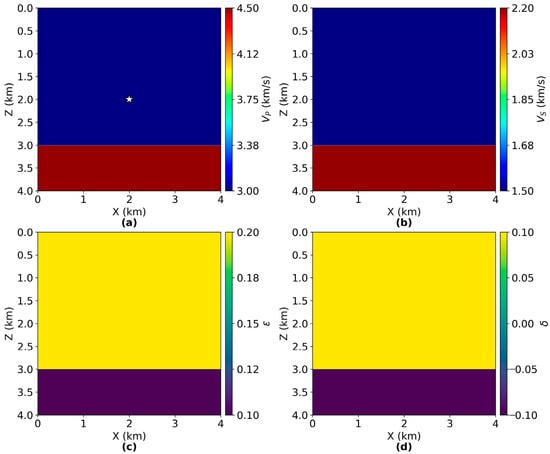
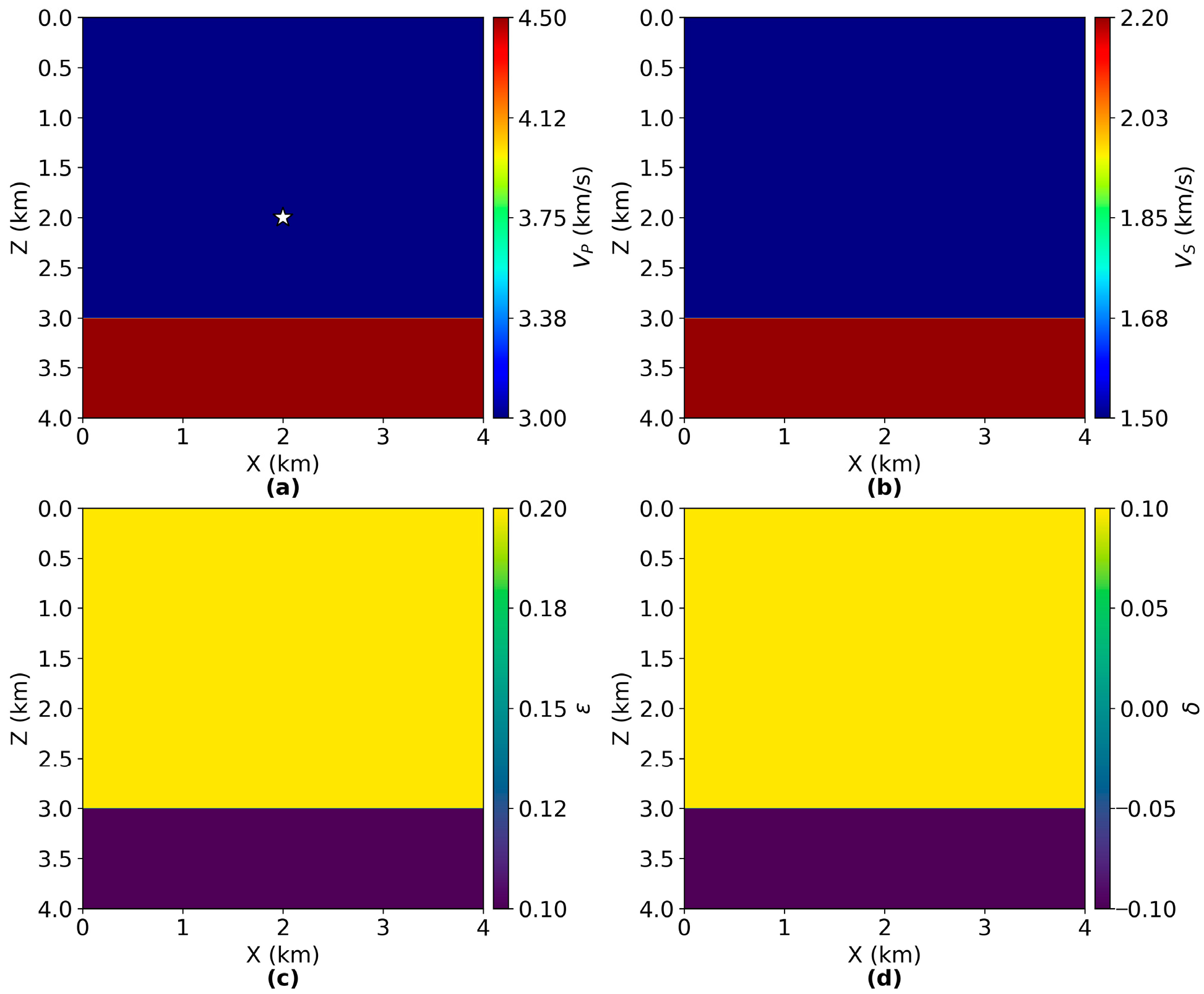
Two-Layer Model. The first model consists of a 400 × 400 grid with 10 m spacing in both directions, representing a 4 km × 4 km domain (Figure 1). The upper layer (0–3.0 km depth) has = 3.0 km/s, = 1.5 km/s, ε = 0.2, and δ = 0.1. The lower layer (3.0–4.0 km depth) has = 4.5 km/s, = 2.2 km/s, ε = 0.1, and δ = −0.1. Density is uniform at ρ = 2.2 g/cm3 throughout both layers. This model tests the method’s ability to handle vertical contrasts in velocity and anisotropic parameters, including a sign change in δ across the interface. The two-layer values were chosen as a minimal layered benchmark with moderate VTI anisotropy; the sign change in δ across the interface was included to test robustness under sharp parameter contrasts.
Figure 1.
Two-layer VTI model configuration. (a) P-wave velocity ; (b) S-wave velocity ; (c) Thomsen parameter ε; (d) Thomsen parameter δ. The white star indicates the source location at (2.0 km, 2.0 km). The interface at 3.0 km depth separates two layers with contrasting anisotropic properties, including a sign reversal in δ.
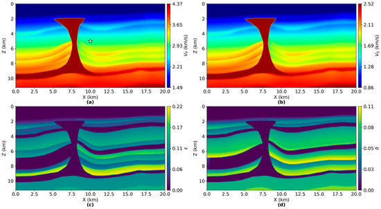
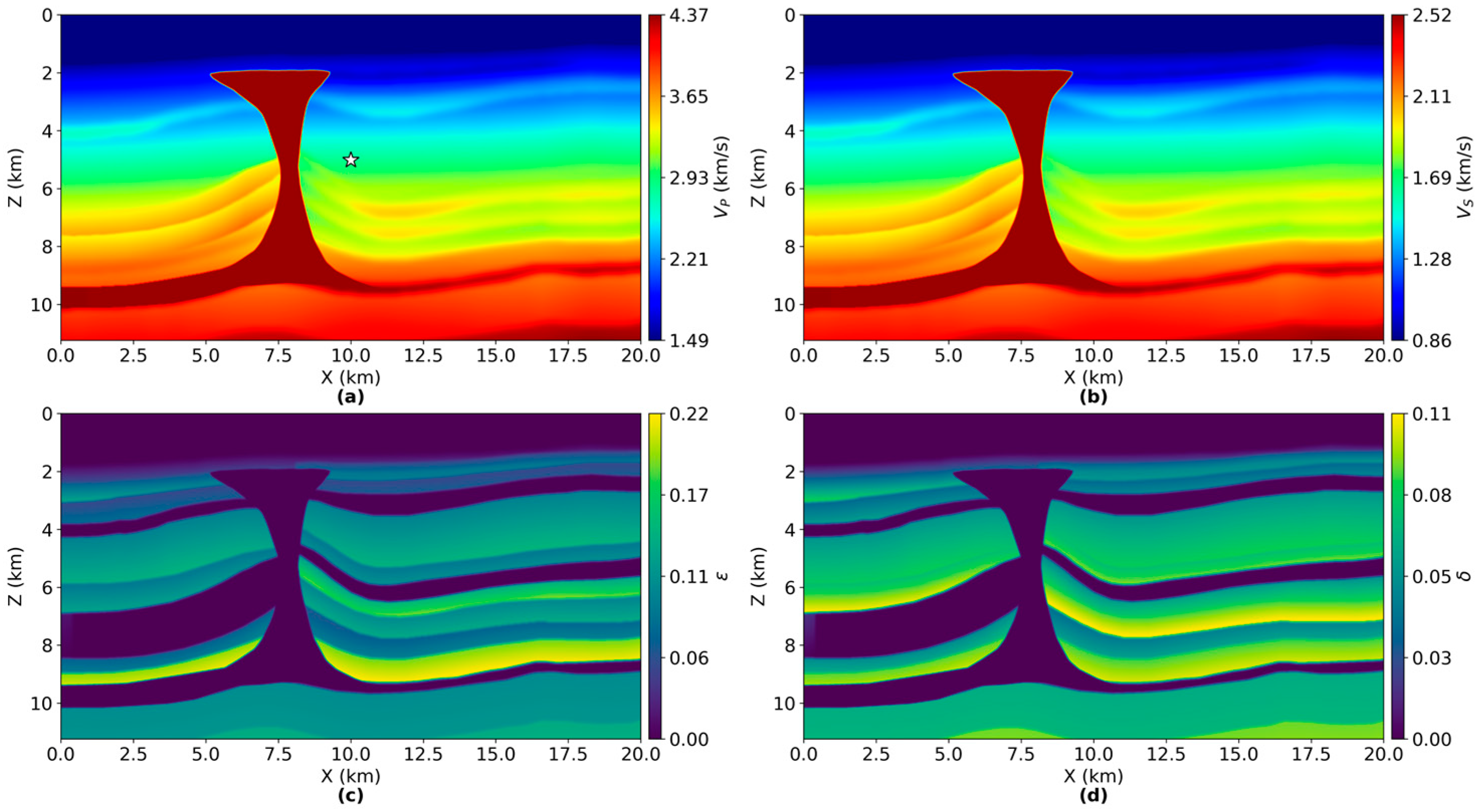
BP VTI Model. The second model uses a subset of the BP 2007 velocity benchmark, covering a 1000 × 562 grid with 20 m spacing (20 km × 11.24 km domain, corresponding to x = 25–45 km from the original model). The pre-defined parameter fields (, , ε, δ) available for the selected BP subset were used without additional manual tuning; the only modification is spatial cropping (x = 25–45 km) to fit the computational budget while preserving the key geological features such as the salt body. Figure 2 shows the spatial distribution of elastic parameters. ranges from 1.49 to 4.37 km/s, and ranges from 0.86 to 2.52 km/s. The Thomsen anisotropy parameters ε and δ range from 0.0 to 0.22 and 0.0 to 0.11, respectively. A salt body penetrates from the surface to approximately 9 km depth near the center of the model, creating strong lateral velocity contrasts.
Figure 2.
BP VTI model configuration. (a) P-wave velocity ; (b) S-wave velocity ; (c) Thomsen parameter ε; (d) Thomsen parameter δ. The white star indicates the source location. The central high-velocity anomaly represents a salt body extending from the surface to approximately 9 km depth.
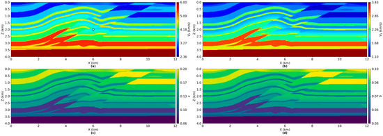
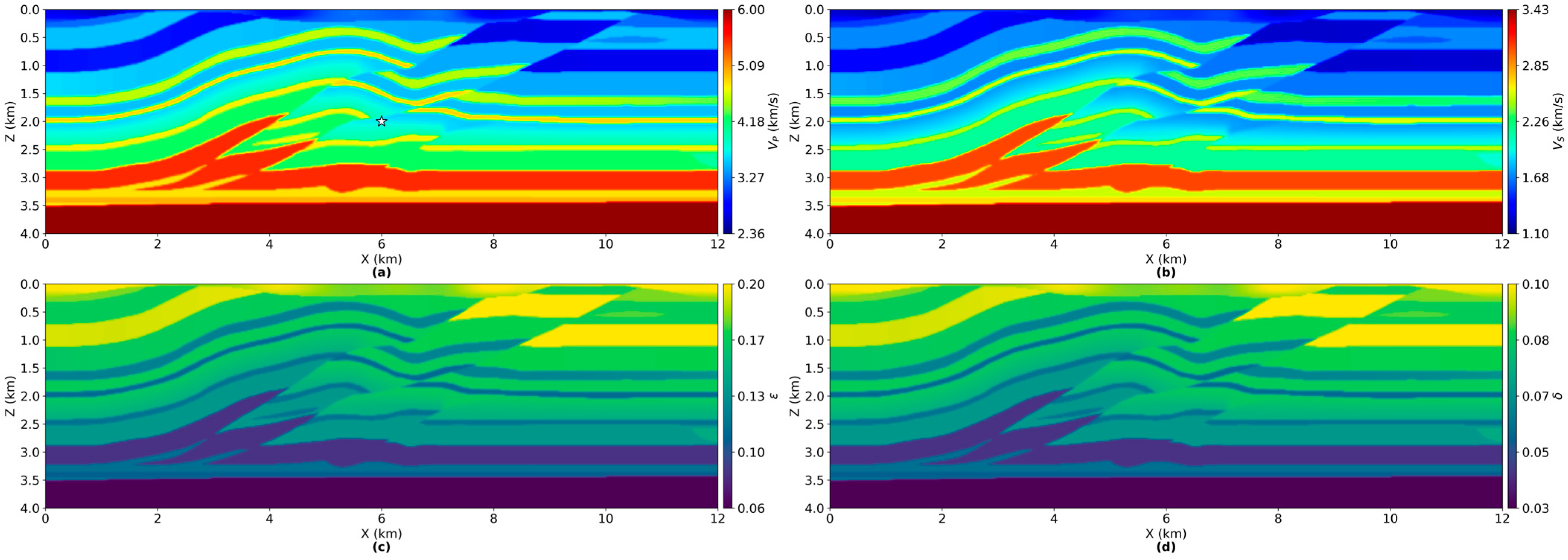
Overthrust VTI Model. To assess robustness in a structurally complex setting, an additional test was performed using a subset of the Overthrust benchmark (600 × 200 grid, 20 m spacing; 12 km × 4 km). The Overthrust VTI model used in this study is shown in Figure 3. Since the public Overthrust model provides only , the remaining elastic and VTI parameters were synthesized using a -dependent proxy mapping so that , , and vary spatially in a manner consistent with the structural features of the model. Specifically, a higher ratio and stronger anisotropy were assigned to lower- regions, while lower and weaker anisotropy were assigned to higher- regions. The parameter ranges were set to , , and . In practice, was normalized to [0, 1] using robust percentile bounds (2nd–98th percentiles) to reduce the influence of outliers, and then applied linear monotonic mappings to the target intervals for /, ε, and δ.
Figure 3.
Overthrust VTI model configuration. (a) P-wave velocity ; (b) S-wave velocity ; (c) Thomsen parameter ε; (d) Thomsen parameter . The white star indicates the source location. The model exhibits strongly deformed and faulted layers with pronounced lateral velocity contrasts, representing a structurally complex overthrust setting.
Elastic wavefields were generated using a fourth-order staggered-grid finite-difference scheme with convolutional perfectly matched layer (CPML) absorbing boundary conditions. A vertical force source with a 15 Hz (two-layer) or 10 Hz (BP and Overthrust) Ricker wavelet was placed at the model center. Snapshots were extracted at t = 1.1 s (two-layer), t = 1.7 s (BP), and t = 0.5 s (Overthrust), capturing both direct and reflected wavefronts.
3.2. Decomposition Quality
Table 2 summarizes the quantitative metrics for both decomposition methods across the three models (two layers, BP, Overthrust). The energy ratio measures total separated energy relative to input energy (ideal value = 1.0). The P and SV fractions indicate the percentage of separated energy attributed to each wave mode. The reconstruction error quantifies the normalized difference between the input wavefield and the sum of separated components. Cross-talk measures the normalized inner product between qP and qSV components (ideal value = 0).
Table 2.
Comparison of decomposition quality metrics for TT and CUR methods.
Both methods yield consistent P/SV energy partitioning, with differences less than 0.8% in fractional energy distribution. However, the TT method achieves substantially lower reconstruction errors (0.094–0.89%) than CUR (1.67–6.44%) and also reduces cross-talk in all three models. These differences reflect the combined effect of (i) adaptive rank selection by TT-cross controlled by a single tolerance and (ii) the residual-orthogonal workflow (Section 2.4.4) used to extract qSV from the post-qP residual; the baseline CUR implementation follows the conventional direct application of qP and qSV projectors to the original wavefield. TT maintains energy ratios close to unity (0.9987–1.0013), whereas CUR shows small deviations above unity (up to 1.0118), indicating minor non-energy-preserving behavior that can arise from approximation and pseudo-inverse errors in the CUR factorization.
The energy ratio for TT remains close to unity (0.9987–1.0013), indicating accurate energy conservation during separation. In contrast, CUR exhibits energy ratios exceeding 1.0 (up to 1.0118), indicating energy overestimation due to non-orthogonality/approximation error. This energy inflation may arise from low-rank approximation errors in the CUR factorization.
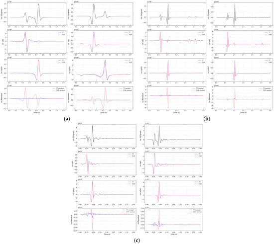
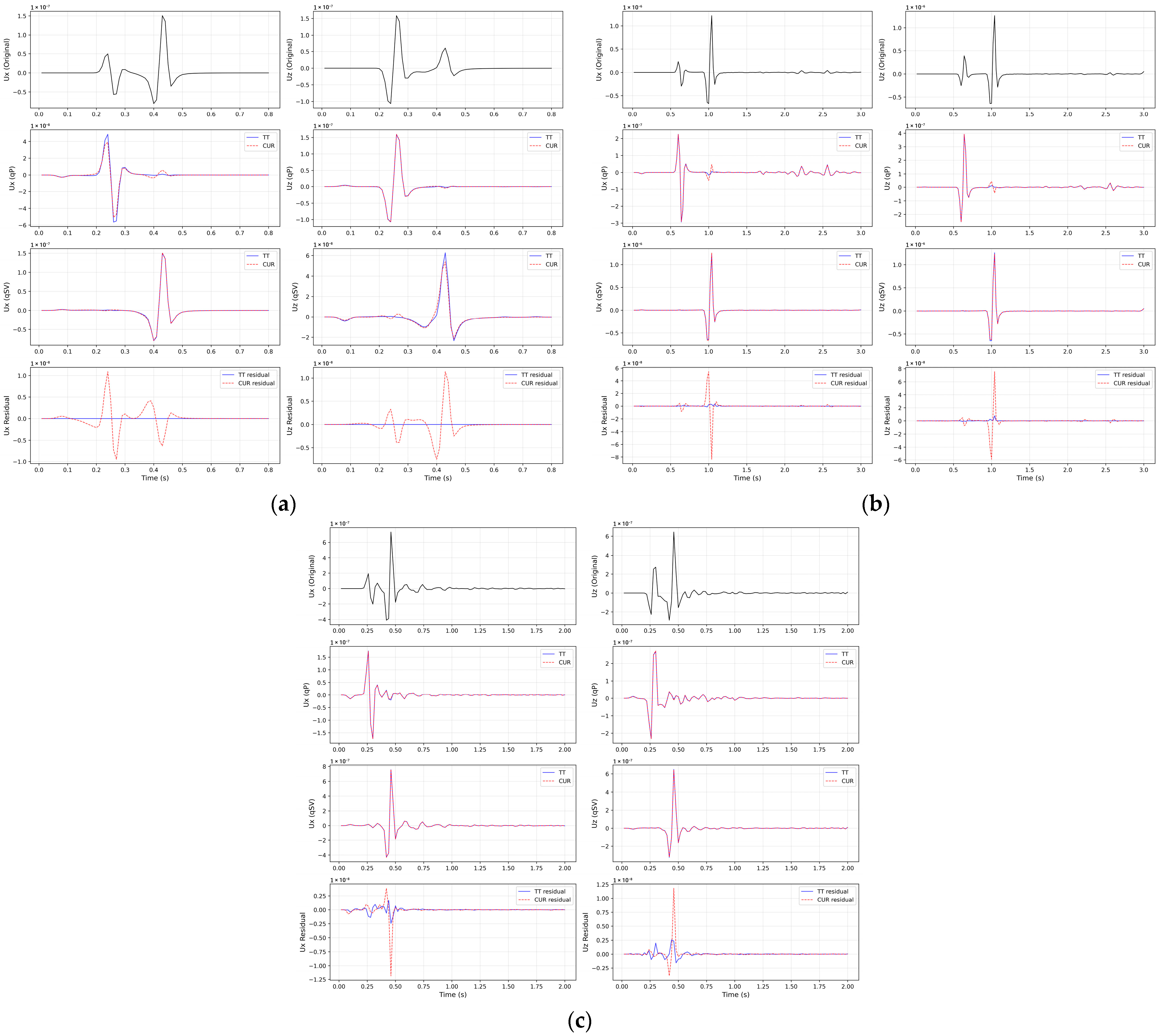
To assess mode-separation quality in the time domain, displacement traces were extracted at a selected receiver location in each model, which resulted in source–receiver offsets of 0.54 km (two-layer), 1.90 km (BP), and 0.89 km (Overthrust). The decomposed qP and qSV components obtained by the TT- and CUR-approximated mixed-domain projectors were compared, and the reconstruction residual was evaluated as a completeness diagnostic. As shown in Figure 4a–c, CUR exhibits larger residual spikes and slightly stronger cross-mode leakage (most noticeably in the BP case), whereas TT remains consistently stable.
Figure 4.
Time-domain trace comparison at a selected receiver for (a) two-layer (offset = 0.54 km), (b) BP (offset = 1.90 km), and (c) Overthrust (offset = 0.89 km) models. Each subfigure is arranged as a 4 × 2 grid: columns show ux (left) and uz (right); rows show original displacement, decomposed qP, decomposed qSV, and the reconstruction residual . Black: original; blue solid: TT; red dashed: CUR.
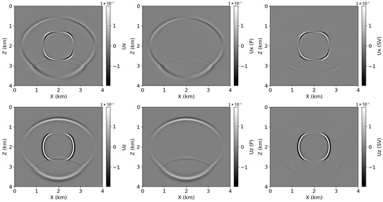
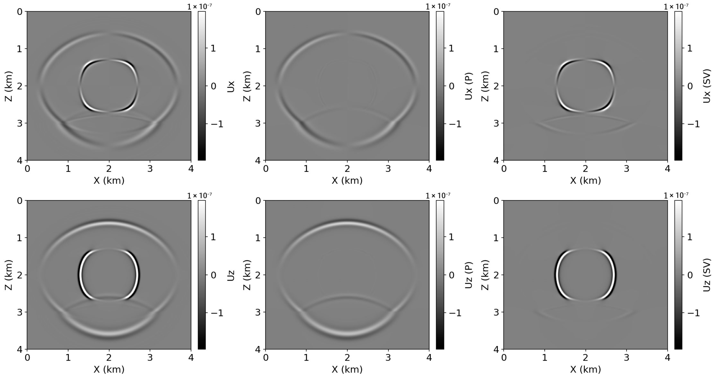
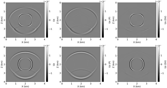
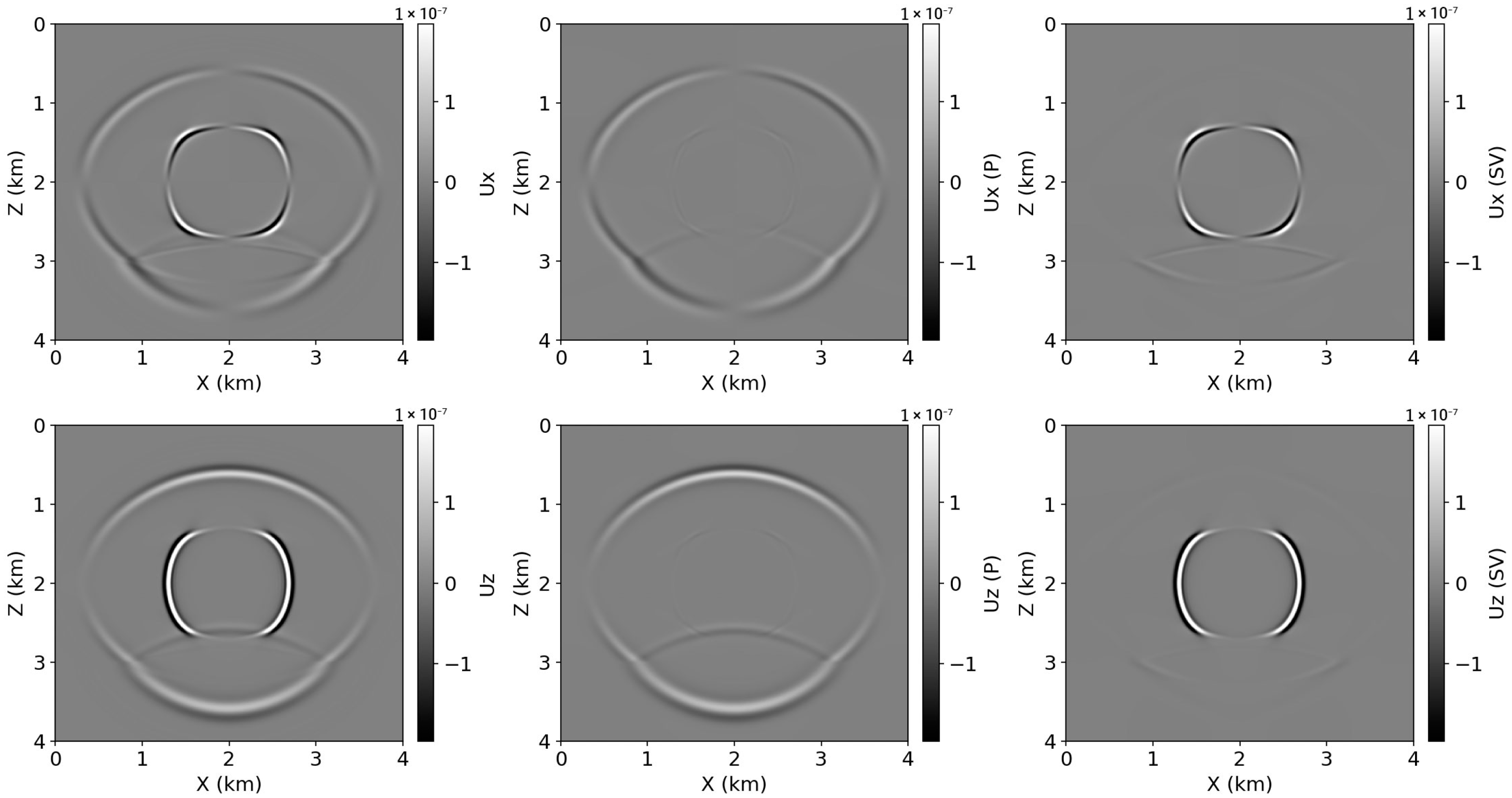
Figure 5 and Figure 6 show the decomposition results for the two-layer model using TT and CUR methods, respectively. The original wavefield (left column) exhibits characteristic qP and qSV wavefronts with elliptical anisotropic moveout. The qP wavefront propagates faster and reaches the layer interface at 3.0 km depth, where reflection, transmission, and mode conversion occur. The TT-decomposed qP component (middle column) cleanly isolates the compressional wave including its reflected and transmitted portions, while the qSV component (right column) captures the slower shear wave with minimal residual qP energy. The CUR decomposition produces qualitatively similar wavefront separation, but the quantitative metrics in Table 2 indicate higher cross-talk and reconstruction error.
Figure 5.
Wavefield decomposition results for the two-layer VTI model at t = 1.1 s using the TT method. Top row: horizontal displacement component (ux); Bottom row: vertical displacement component (uz). Left column: original wavefield; Middle column: separated qP wave; Right column: separated qSV wave.
Figure 6.
Wavefield decomposition results for the two-layer VTI model at t = 1.1 s using the CUR method. Top row: horizontal displacement component (ux); Bottom row: vertical displacement component (uz). Left column: original wavefield; Middle column: separated qP wave; Right column: separated qSV wave.
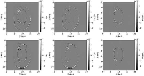
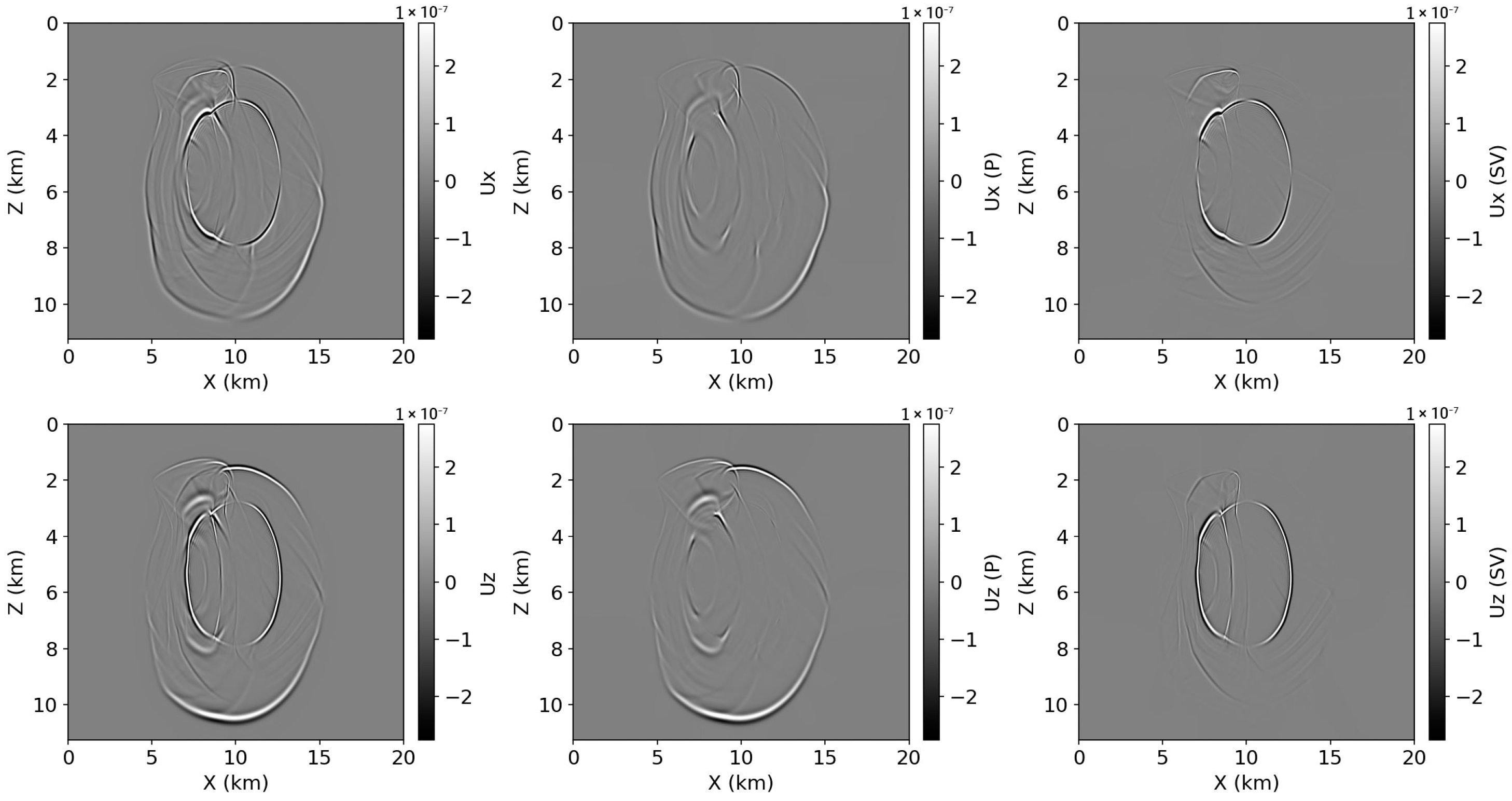
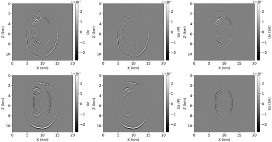
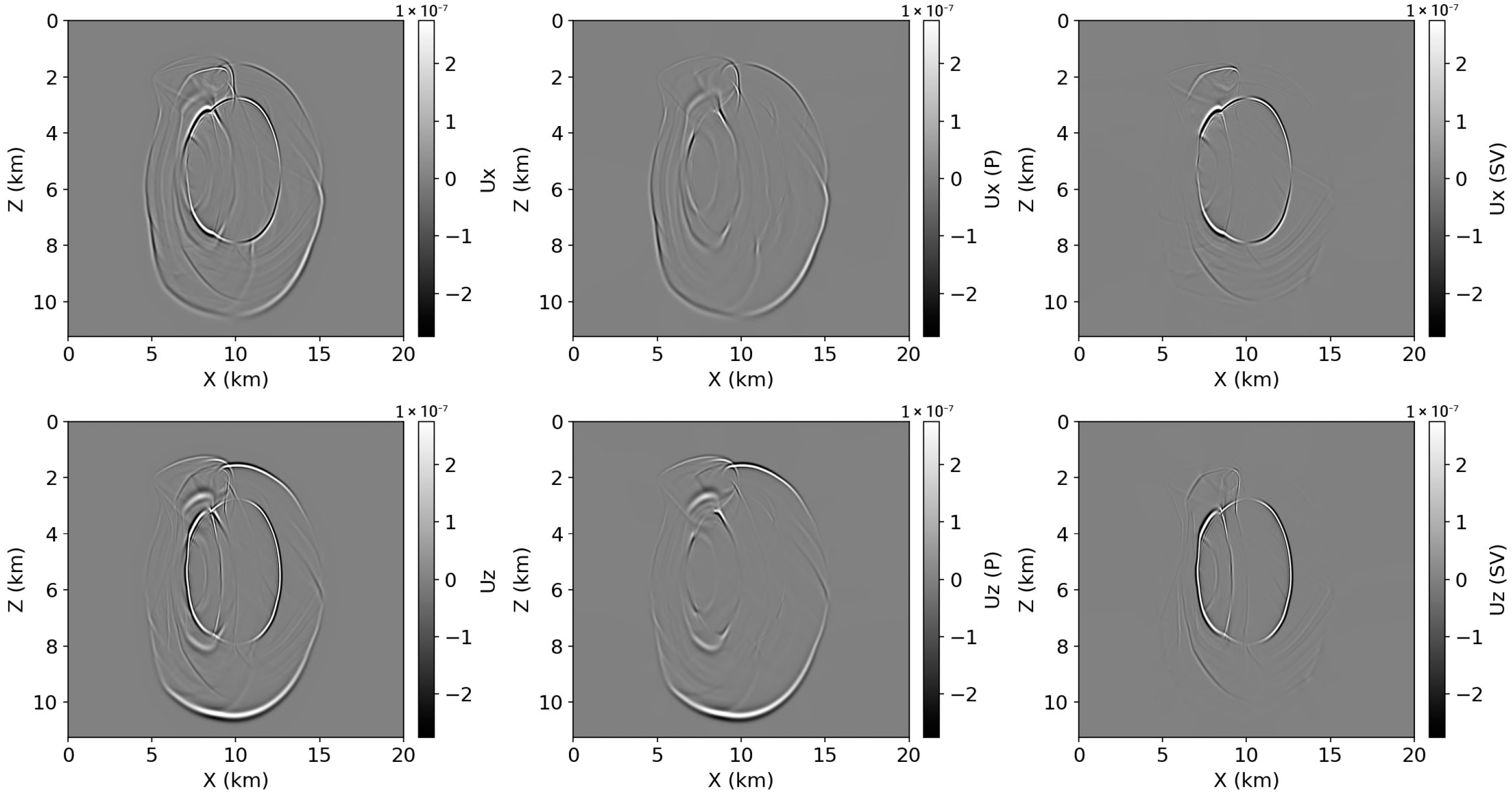
Figure 7 and Figure 8 present the BP model results for TT and CUR methods, respectively. The heterogeneous velocity structure produces complex wave interactions including multiple reflections, head waves along the salt flanks, and mode conversions at layer interfaces. The central salt body causes significant wavefront distortion and amplitude focusing. The TT method successfully separates these overlapping arrivals, maintaining sharp wavefront definition even in regions of strong lateral velocity gradients surrounding the salt body. The qP component clearly shows the direct wave and multiple reflections from the complex layered structure, while the qSV component isolates the converted waves and direct shear arrivals. Both methods produce visually similar separation results, demonstrating that either approach can provide useful wavefield decomposition for qualitative interpretation purposes.
Figure 7.
Wavefield decomposition results for the BP VTI model at t = 1.7 s using the TT method. Top row: horizontal displacement component (ux); Bottom row: vertical displacement component (uz). Left column: original wavefield; Middle column: separated qP wave; Right column: separated qSV wave.
Figure 8.
Wavefield decomposition results for the BP VTI model at t = 1.7 s using the CUR method. Top row: horizontal displacement component (ux); Bottom row: vertical displacement component (uz). Left column: original wavefield; Middle column: separated qP wave; Right column: separated qSV wave.
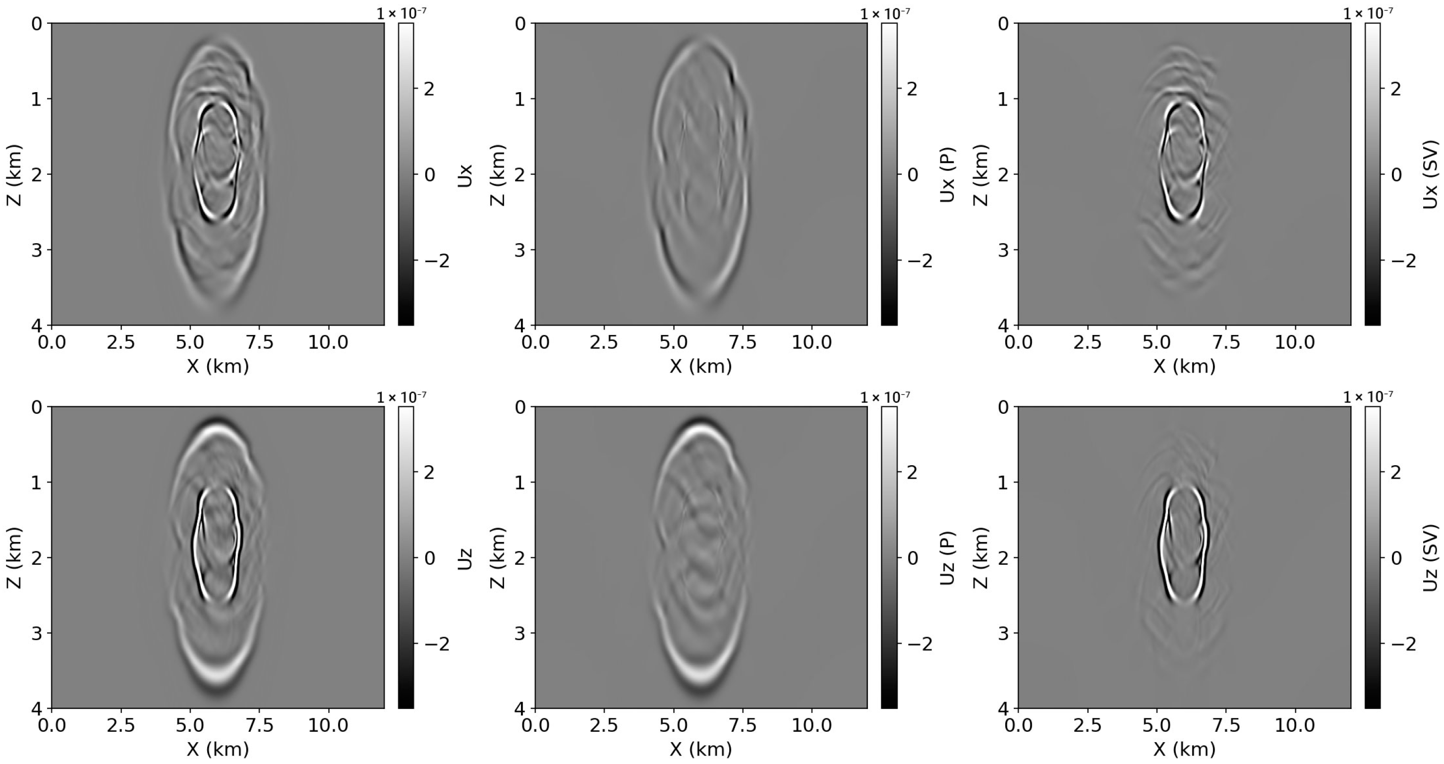
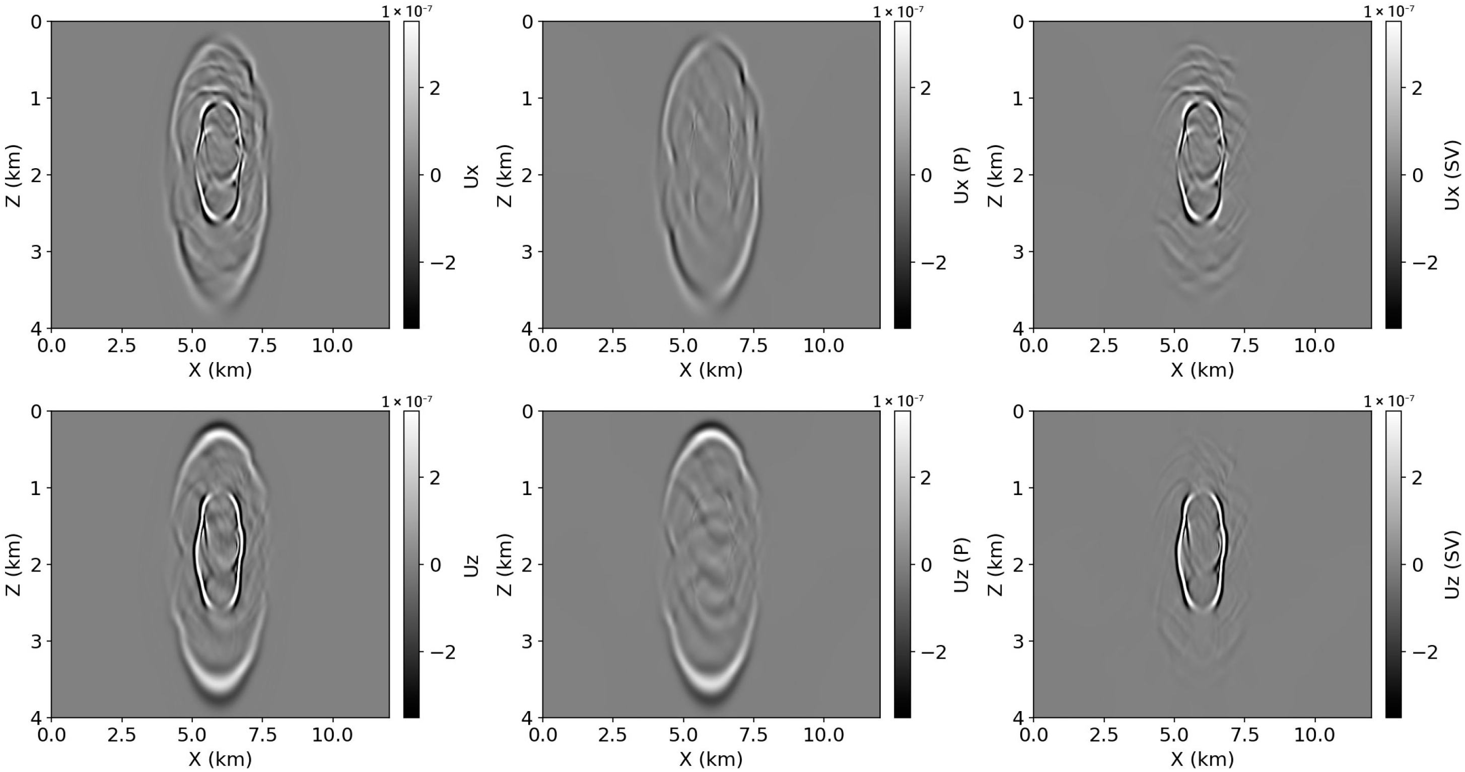
Figure 9 and Figure 10 show the Overthrust model results for the TT and CUR methods, respectively. The Overthrust model contains strongly deformed layers and sharp lateral contrasts, which generate complicated scattering, overlapping arrivals, and pronounced mode conversions. Despite the increased structural complexity, the TT method preserves coherent qP and qSV wavefronts with reduced residual leakage between the modes, consistent with the quantitative trends in Table 2 (lower reconstruction error and cross-talk compared to CUR). The CUR method also separates the main wave modes, but exhibits relatively stronger residual interference and less stable cancelation of leakage in regions with abrupt structural changes.
Figure 9.
Wavefield decomposition results for the Overthrust VTI model at t = 0.5 s using the TT method. Top row: horizontal displacement component (ux); Bottom row: vertical displacement component (uz). Left column: original wavefield; Middle column: separated qP wave; Right column: separated qSV wave.
Figure 10.
Wavefield decomposition results for the Overthrust VTI model at t = 0.5 s using the CUR method. Top row: horizontal displacement component (ux); Bottom row: vertical displacement component (uz). Left column: original wavefield; Middle column: separated qP wave; Right column: separated qSV wave.
3.3. Computational Performance
Table 3 compares the computational performance of the proposed TT-based method and the conventional CUR-based method under different model sizes and hardware configurations. The TT method was evaluated on both GPU (NVIDIA GeForce RTX 4090, 24 GB) and CPU (AMD Ryzen Threadripper PRO 5995WX, 64 cores), while the CUR method was executed on a single CPU thread using Intel Fortran with MKL optimization. Although the CUR implementation could potentially benefit from multi-threading, the original single-threaded code from Cheng and Fomel (2014) [10] was employed with rank parameters m = n = 3 for fair comparison with the published method. To investigate scalability, a homogeneous VTI model with a 2000 × 1000 grid (20 m spacing) was additionally tested.
Table 3.
Computational time comparison (in seconds).
For small-to-moderate grids, the CUR baseline is faster than TT, even though it is executed using a single CPU thread. On the two-layer model (400 × 400), CUR completes in 2.65 s, compared to 9.0 s for TT (CUDA). A similar trend is observed for the BP model (1000 × 562), where CUR requires 10.7 s and TT (CUDA) requires 19.0 s. The Overthrust model (600 × 200) further confirms this behavior: CUR completes in 1.27 s, whereas TT (CUDA) requires 10.6 s. This advantage for smaller problems is consistent with the CUR method’s relatively simple algebraic structure and its reliance on highly optimized dense linear-algebra routines.
However, the scalability trend reverses for larger grids. On the homogeneous 2000 × 1000 test, TT (CUDA) completes in 43.9 s, while CUR requires 66.8 s, making TT 1.5× faster. This crossover reflects the more favorable scaling of the TT framework when the effective TT rank remains bounded by the tolerance and rank cap, while GPU acceleration becomes increasingly efficient for large FFTs and tensor operations. In contrast, the CUR implementation requires repeated matrix operations whose cost grows less favorably with problem size, and it does not benefit from GPU parallelism in the present baseline setup.
The CPU results show that TT benefits substantially from GPU acceleration. Across all tested cases, TT (CPU) remains slower than TT (CUDA), requiring 43.8–210.2 s versus 9.0–43.9 s on GPU. Even though TT (CPU) can be used when GPU resources are unavailable, these timings indicate that a GPU-equipped workstation is preferable for routine use of the TT framework.
Overall, the proposed TT method achieves improved decomposition accuracy (Table 2) without sacrificing practicality in runtime. While CUR can be faster on small grids, the TT implementation becomes faster on sufficiently large grids, where its scaling behavior and GPU utilization dominate the runtime.
4. Discussion
4.1. Accuracy Advantages of TT Decomposition
The accuracy comparison discussed in this section is based on the three 2D VTI synthetic tests reported in Section 3.1 and summarized quantitatively in Table 2: the two-layer benchmark with a sharp vertical contrast (including a sign change in δ), the heterogeneous BP 2007 subset featuring a complex salt-driven lateral velocity contrast, and the Overthrust-based model in which elastic/VTI parameters were synthesized from the provided field via a monotonic -dependent proxy mapping. For each model, both decomposition approaches were applied to the same simulated wavefield snapshots, and separation quality was evaluated using energy ratio, P/SV energy fractions, cross-talk, and reconstruction error.
Across these three tests, TT-based decomposition consistently yields higher fidelity than the conventional CUR approach. The reconstruction errors for TT remain below 1% (0.094–0.89%), whereas CUR shows substantially larger errors (1.67–6.44%), indicating a clear improvement in wavefield consistency when the separated components are recombined. The advantage is especially pronounced in the two-layer benchmark, where the sharp parameter discontinuity and the sign reversal of δ provide a stringent stress test for polarization-based projectors. In the same setting, TT reduces cross-talk by roughly two orders of magnitude compared to CUR (Table 2), demonstrating more stable suppression of mode leakage.
This accuracy gain is attributable to two algorithmic characteristics of the TT framework. First, TT-cross adaptively determines the effective approximation ranks from a single tolerance parameter τ, which helps maintain a uniform approximation quality for the mixed-domain decomposition operator even in regions where polarization vectors vary rapidly due to strong anisotropy or sharp contrasts. By contrast, CUR relies on a fixed low-rank parameterization; in the comparison, the published setting m = n = 3 was adopted to maintain consistency with the conventional method [10]. Second, the residual-orthogonal strategy (Section 2.4.4) constructs the qSV component from the residual wavefield after qP removal, rather than projecting the original wavefield onto both subspaces independently. This sequential formulation reduces double-counting and stabilizes separation in regions where the qP and qSV polarization directions are not perfectly orthogonal in practice, which is reflected directly by the reduced cross-talk values.
Energy consistency provides additional evidence of improved stability. TT maintains energy ratios very close to unity across all three models (0.9987–1.0013), whereas CUR can exceed 1.0, indicating small but systematic deviations from energy-preserving separation. Although both methods produce similar overall P/SV energy partitioning, the lower reconstruction error and reduced cross-talk obtained by TT indicate that the separated wavefields better preserve the physical structure of the underlying modes, particularly under strong heterogeneity or sharp parameter transitions.
These improvements in separation fidelity are practically relevant because mode leakage can translate into non-physical interference in downstream elastic imaging workflows. In particular, when separated wavefields are used within least-squares migration or related multi-component imaging procedures, reduced cross-talk and stable energy partitioning are desirable to mitigate artifact contamination and improve the reliability of subsequent updates or compensation steps. This is consistent with the broader context of high-resolution seismic imaging technology [3] and with recent ocean-bottom dual-sensor least-squares RTM workflows that incorporate acoustic/elastic coupling and mode-separated wavefields, including joint acoustic and decoupled-elastic LSRTM [25] and Q-compensated elastic LSRTM based on acoustic and separated-viscoelastic coupling equations [26].
4.2. Computational Considerations
The computational results show that the relative efficiency of TT and CUR methods depends on problem size. For smaller grids, CUR is substantially faster than TT (CUDA): 8.3× for Overthrust (600 × 200) and 3.4× for the two-layer model (400 × 400). For the medium-sized BP grid (1000 × 562), this gap narrows to 1.8×. For larger grids (2000 × 1000), TT (CUDA) becomes 1.5× faster than CUR.
This size-dependent behavior arises from the different computational structures of the two methods. The CUR method relies on simple matrix-matrix multiplications that are highly optimized through Intel MKL. For smaller problems, this simplicity outweighs the overhead of TT-cross construction and core tensor management. However, as problem size increases, the TT framework’s complexity for wavefield application becomes advantageous, where R is the TT-rank and Ns is the total grid size. The rank R remains bounded by the tolerance parameter τ regardless of grid size, while Ns grows quadratically with grid dimension.
GPU acceleration plays an important role in TT performance. The 4.1–5.5× speedup from CPU to GPU reflects efficient parallelization of FFT operations and tensor contractions. Larger problems achieve better GPU utilization because the increased data volume amortizes memory transfer overhead and fills more parallel processing units.
The single-threaded CUR implementation used in this study represents the original published code. Multi-threaded or GPU-accelerated CUR implementations could reduce the performance gap for smaller problems. However, the fundamental scaling behavior—where TT becomes faster for larger grids—would remain unchanged because it stems from algorithmic complexity rather than implementation details.
4.3. Scalability to Three-Dimensional Problems
Although the numerical validation in this paper is presented in 2D, the primary motivation for adopting a tensor-train (TT) representation is tied to three-dimensional (3D) problems, where the decomposition operator naturally becomes higher-dimensional. In 3D elastic VTI media, the mixed-domain decomposition operator depends on x = (x, y, z) and k = (kx, ky, kz), forming a 6D object . This increase in dimensionality is not a minor extension: a matrix view requires flattening multi-index coordinates into two very long axes, which rapidly escalates memory traffic and computational cost even when a low-rank approximation is used. The TT format is attractive in this setting because it preserves the multi-index structure explicitly and compresses the operator as a chain of low-rank cores along tensor dimensions, rather than forcing a high-dimensional operator into a 2D matrix layout. As a result, the dominant computational patterns shift from large dense matrix operations toward structured tensor contractions and FFT-based mixed-domain evaluations, which are better aligned with high-dimensional operators.
Three-dimensional mode separation also introduces algorithmic requirements that are less pronounced in 2D. First, 3D elastic decomposition involves three wave modes (qP, qSV, qSH), and practical separation must manage mutual leakage stably. The residual-orthogonal strategy described in Section 2.4.4 extends naturally as a sequential separation scheme (qP removed first, followed by qSV from the residual, and then qSH from the remaining residual), directly targeting mode coupling when polarization directions are not perfectly orthogonal numerically. Second, physical labeling and continuity control of eigenvectors becomes more delicate in 3D because polarization vectors must be tracked consistently over k, including near symmetry-axis configurations where degeneracy or near-degeneracy may occur. Robust 3D implementations therefore require physically motivated labeling rules (e.g., alignment with for qP and a consistent transverse reference for qSH) and explicit sign/phase continuity handling to avoid artificial polarity flips that can propagate into decomposed wavefields.
It is also informative to relate the proposed TT framework to recent 3D separation methods, such as the 3D pseudo-Helmholtz decomposition [27]. Pseudo-Helmholtz–type approaches can provide effective 3D mode separation, while their implementation for production-scale grids may involve substantial operator applications and/or auxiliary solves. In contrast, the proposed TT framework focuses on operator compression: by representing the mixed-domain decomposition operator in the TT format, the storage scales favorably with dimension and the operator can be applied efficiently without explicitly forming large dense objects. This difference in computational workflow helps explain why TT becomes increasingly attractive as the grid size and dimensionality grow.
Beyond computational scaling, this capability has direct practical relevance to field-scale hydrocarbon exploration and reservoir characterization, where 3D anisotropic wavefields and large grids are standard. The proposed TT-based decomposition can be integrated as a scalable building block in workflows such as anisotropic RTM/LSRTM, where qP-focused imaging may mitigate P–SV crosstalk and improve interpretability in complex overburdens (e.g., strongly layered VTI or subsalt/sub-basalt settings). In addition, within elastic/VTI full-waveform inversion, mode-separated wavefields can be used to form more physically consistent gradients and reduce parameter trade-offs, stabilizing updates of velocities and Thomsen parameters when targeting reservoir-scale resolution. For reservoir characterization, cleaner mode components also support amplitude/attribute analyses and time-lapse (4D) monitoring by reducing contamination between P- and S-related responses.
Finally, a comprehensive 3D benchmark requires careful experimental design (model selection, snapshot configuration, continuity-controlled labeling, and consistent metrics) and is therefore treated as a dedicated extension rather than being appended superficially to the present 2D validation.
4.4. Limitations and Future Work
Several limitations of the present study should be acknowledged, together with clear directions for extending the framework beyond the current 2D validation. First, the TT-cross approximation may exhibit run-to-run variability because its convergence and the final TT representation can depend on the initial index selection. While the decomposition accuracy is primarily controlled by the tolerance parameter, applications requiring strict reproducibility would benefit from deterministic initialization schemes (e.g., fixed seed policies and prescribed index schedules) or from stabilized construction strategies (e.g., repeated builds followed by consistency checks on selected operator slices).
Second, the current implementation assumes time-independent medium parameters when constructing the mixed-domain decomposition operators. In workflows where medium properties evolve—such as time-lapse monitoring, iterative inversion updates, or scenarios involving time-varying effective parameters—operator reconstruction (or efficient operator updates) becomes an additional computational burden. A practical extension is to investigate incremental or warm-start TT updates when parameter perturbations are moderate, or to design a caching strategy that reuses previously built tensor cores whenever local changes are confined.
Third, the scope is restricted to VTI symmetry. Many realistic settings exhibit lower symmetries (e.g., orthorhombic media), tilted TI, or general anisotropy, where polarization behavior is more complex and eigenvalue/eigenvector structures can involve degeneracies and singularities. Extending the proposed framework to these media classes requires a robust polarization labeling strategy in 3D -space, including continuity control and physically consistent sign/phase conventions. In addition, lower-symmetry media increase the sensitivity of labeling near problematic regions of -space, so practical extensions should include explicit safeguards for near-degenerate eigenpairs and stability checks for projector construction.
Fourth, the present study is limited to elastic VTI media. A natural extension is wavefield decomposition in viscoelastic or attenuated TI media, where phase velocities and polarization vectors can become frequency dependent and complex-valued. Since the proposed workflow constructs the mixed-domain decomposition operator through function evaluations and compresses it in TT form, the same pipeline can, in principle, be extended by adopting attenuative constitutive descriptions and computing complex-valued polarization-based projectors. This direction requires careful numerical treatment of eigenvector phase continuity and support for complex-valued TT representations, as well as validation against established attenuated qP/qSV formulations [28].
Finally, while Section 4.3 motivates why TT representations are particularly appealing in 3D, the present manuscript does not provide a full 3D benchmark suite and therefore cannot claim comprehensive 3D validation. A dedicated 3D evaluation should be designed around (i) three-mode separation (qP, qSV, qSH) with continuity-controlled polarization labeling in (kx, ky, kz), (ii) representative 3D models spanning layered TI, strong heterogeneity, and structurally complex settings, and (iii) consistent quantitative metrics (energy consistency, cross-talk among all mode pairs, and reconstruction error) measured over large-scale grids. Such a study would clarify practical crossover behavior (accuracy and runtime) and establish integration guidelines for 3D anisotropic RTM/LSRTM and elastic/VTI inversion pipelines, where separation quality and stability directly affect imaging artifacts and gradient reliability.
5. Conclusions
This paper presented a tensor-train decomposition framework for elastic wavefield decomposition in VTI media. The proposed method formulates the Christoffel-based projection operator as a four-dimensional tensor and constructs its compressed TT representation using the TT-cross algorithm.
The proposed TT method consistently improved separation fidelity across three 2D VTI tests (two-layer, BP 2007 subset, and an Overthrust-based model). Reconstruction errors for TT remained below 1% (0.094–0.89%), whereas CUR showed larger errors (1.67–6.44%), yielding a 4–46× improvement, with markedly reduced cross-talk (nearly two orders of magnitude in the sharp-contrast two-layer case) and energy ratios close to unity for TT (0.9987–1.0013) compared with CUR (up to 1.0118). The improved stability primarily reflects the TT-based pipeline used in this study, which performs qSV extraction from the post-qP residual (residual-orthogonal strategy). In contrast, the CUR baseline applies direct projection to the original wavefield. Therefore, the comparison here should be interpreted as an end-to-end pipeline comparison rather than an isolated assessment of the low-rank approximator itself.
Computational experiments revealed size-dependent performance characteristics consistent with the updated benchmark suite. For small-to-moderate grids (e.g., 400 × 400, 1000 × 562, and 600 × 200), the CUR baseline remained faster than TT (CUDA). However, the scalability trend reversed on the larger-grid test (2000 × 1000), where TT (CUDA) became faster than CUR (about 1.5×), reflecting the more favorable scaling of the TT framework and improved GPU utilization for large FFT/tensor operations. TT also benefited substantially from GPU acceleration compared with CPU execution, indicating that a GPU-equipped workstation is preferable for routine application of the TT framework.
Finally, the TT framework offers scalability advantages for three-dimensional problems, where the decomposition operator becomes a 6D tensor. The storage complexity scaling linearly with dimension——makes TT suitable for 3D elastic wavefield decomposition at scales impractical for conventional methods, and the single tolerance parameter τ simplifies workflow integration by eliminating manual rank selection.
Future work will extend the framework to 3D problems with three wave modes (qP, qSV, qSH), integrate the decomposition into elastic RTM and FWI workflows, and develop extensions for lower-symmetry anisotropic media.
Funding
This research was supported by a National Research Foundation of Korea (NRF) grant, funded by the Korea government (MSIT) (No. 2023-00212423).
Institutional Review Board Statement
Not applicable.
Informed Consent Statement
Not applicable.
Data Availability Statement
The original contributions presented in this study are included in the article. Further inquiries can be directed to the corresponding author.
Acknowledgments
The anonymous reviewers and the associated Editor are appreciated for their constructive comments that helped improve the quality of the manuscript. The 2007 BP anisotropic velocity benchmark dataset, provided courtesy of BP Exploration Operation Company Limited, was used for numerical validation. The SEG/EAGE Overthrust model was used as the structural basis for the synthesized VTI test case. The CUR decomposition code for comparison was based on the low-rank approximation method of Cheng and Fomel (2014). During the preparation of this manuscript, the author used Claude (Anthropic, claude-3.5-sonnet) for the purposes of drafting and editing text. The author has reviewed and edited the output and takes full responsibility for the content of this publication.
Conflicts of Interest
The author declares no conflicts of interest.
References
- Yan, J.; Sava, P. Elastic Wave-Mode Separation for VTI Media. Geophysics 2009, 74, WB19–WB32. [Google Scholar] [CrossRef] [Scilit]
- Du, Q.; Zhu, Y.; Ba, J. Polarity Reversal Correction for Elastic Reverse Time Migration. Geophysics 2012, 77, S31–S41. [Google Scholar] [CrossRef] [Scilit]
- Li, Z.-C.; Qu, Y.-M. Research Progress on Seismic Imaging Technology. Pet. Sci. 2022, 19, 128–146. [Google Scholar] [CrossRef] [Scilit]
- Mora, P. Nonlinear Two-Dimensional Elastic Inversion of Multioffset Seismic Data. Geophysics 1987, 52, 1211–1228. [Google Scholar] [CrossRef] [Scilit]
- Aki, K.; Richards, P.G. Quantitative Seismology; University Science Books: Melville, NY, USA, 2002; ISBN 978-0-935702-96-5. [Google Scholar]
- Zhu, H. Elastic Wavefield Separation Based on the Helmholtz Decomposition. Geophysics 2017, 82, S173–S183. [Google Scholar] [CrossRef] [Scilit]
- Zhang, Q.; McMechan, G.A. 2D and 3D Elastic Wavefield Vector Decomposition in the Wavenumber Domain for VTI Media. Geophysics 2010, 75, D13–D26. [Google Scholar] [CrossRef] [Scilit]
- Thomsen, L. Weak Elastic Anisotropy. Geophysics 1986, 51, 1954–1966. [Google Scholar] [CrossRef] [Scilit]
- Tsvankin, I. Seismic Signatures and Analysis of Reflection Data in Anisotropic Media; SEG Books: Houston, TX, USA, 2012; ISBN 978-1-56080-299-0. [Google Scholar]
- Cheng, J.; Fomel, S. Fast Algorithms for Elastic-Wave-Mode Separation and Vector Decomposition Using Low-Rank Approximation for Anisotropic Media. Geophysics 2014, 79, C97–C110. [Google Scholar] [CrossRef] [Scilit]
- Song, X.; Fomel, S.; Ying, L. Lowrank Finite-Differences and Lowrank Fourier Finite-Differences for Seismic Wave Extrapolation in the Acoustic Approximation. Geophys. J. Int. 2013, 193, 960–969. [Google Scholar] [CrossRef] [Scilit]
- Sun, J.; Fomel, S.; Ying, L. Low-Rank One-Step Wave Extrapolation for Reverse Time Migration. Geophysics 2016, 81, S39–S54. [Google Scholar] [CrossRef] [Scilit]
- Fomel, S.; Ying, L.; Song, X. Seismic Wave Extrapolation Using Lowrank Symbol Approximation. Geophys. Prospect. 2013, 61, 526–536. [Google Scholar] [CrossRef] [Scilit]
- Zhang, L.; Liu, L.; Niu, F.; Zuo, J.; Shuai, D.; Jia, W.; Zhao, Y. A Novel and Efficient Engine for P-/S-Wave-Mode Vector Decomposition for Vertical Transverse Isotropic Elastic Reverse Time Migration. Geophysics 2022, 87, S185–S207. [Google Scholar] [CrossRef] [Scilit]
- Oseledets, I.V. Tensor-Train Decomposition. SIAM J. Sci. Comput. 2011, 33, 2295–2317. [Google Scholar] [CrossRef] [Scilit]
- Oseledets, I.; Tyrtyshnikov, E. TT-Cross Approximation for Multidimensional Arrays. Linear Algebra Appl. 2010, 432, 70–88. [Google Scholar] [CrossRef] [Scilit]
- Grasedyck, L.; Kressner, D.; Tobler, C. A Literature Survey of Low-Rank Tensor Approximation Techniques. GAMM-Mitteilungen 2013, 36, 53–78. [Google Scholar] [CrossRef] [Scilit]
- Hackbusch, W. Tensor Spaces and Numerical Tensor Calculus; Springer Science & Business Media: Berlin/Heidelberg, Germany, 2012; ISBN 978-3-642-28027-6. [Google Scholar]
- Liu, D.; Sacchi, M.D.; Chen, W. Efficient Tensor Completion Methods for 5-D Seismic Data Reconstruction: Low-Rank Tensor Train and Tensor Ring. IEEE Trans. Geosci. Remote Sens. 2022, 60, 5916317. [Google Scholar] [CrossRef] [Scilit]
- Cavalcante, Q.; Porsani, M.J. Prestack Seismic Data Reconstruction and Denoising by Orientation-Dependent Tensor Decomposition. Geophysics 2021, 86, V107–V117. [Google Scholar] [CrossRef] [Scilit]
- Carcione, J.M. Wave Fields in Real Media: Wave Propagation in Anisotropic, Anelastic, Porous and Electromagnetic Media; Elsevier: Amsterdam, The Netherlands, 2022; ISBN 978-0-323-98359-4. [Google Scholar]
- Kolda, T.G.; Bader, B.W. Tensor Decompositions and Applications. SIAM Rev. 2009, 51, 455–500. [Google Scholar] [CrossRef] [Scilit]
- Jeong, W.; Tsingas, C.; Kim, Y.S. Enhanced Elastic Wavefield Separation Using Local Orthogonalization Filtering with Applications in Elastic Modelling and Inversion. J. Appl. Geophys. 2019, 160, 131–143. [Google Scholar] [CrossRef] [Scilit]
- Chen, Y.; Fomel, S. Random Noise Attenuation Using Local Signal-and-Noise Orthogonalization. Geophysics 2015, 80, WD1–WD9. [Google Scholar] [CrossRef] [Scilit]
- Qu, Y.; Li, J.; Li, Y.; Li, Z. Joint Acoustic and Decoupled-Elastic Least-Squares Reverse Time Migration for Simultaneously Using Water-Land Dual-Detector Data. IEEE Trans. Geosci. Remote Sens. 2023, 61, 5909511. [Google Scholar] [CrossRef] [Scilit]
- Li, J.; Qu, Y.; Li, Y.; Huang, C.; Li, Z. Ocean Bottom Dual-Sensor Q-Compensated Elastic Least-Squares Reverse Time Migration Based on Acoustic and Separated-Viscoelastic Coupling Equations. Geophysics 2024, 89, S155–S173. [Google Scholar] [CrossRef] [Scilit]
- Zuo, J.; Niu, F.; Liu, L.; Da, S.; Zhang, H.; Yang, J.; Zhang, L.; Zhao, Y. 3D Anisotropic P- and S-Mode Wavefields Separation in 3D Elastic Reverse-Time Migration. Surv. Geophys. 2022, 43, 673–701. [Google Scholar] [CrossRef] [Scilit]
- Huang, R.; Wang, Z.; Song, G.; Xiang, Y.; Zhao, L.; Chen, P. Decoupled Approximate qP- and qSV-wave Equations in Attenuated Transversely Isotropic Media. Geophys. Prospect. 2024, 72, 3495–3510. [Google Scholar] [CrossRef] [Scilit]

Disclaimer/Publisher’s Note: The statements, opinions and data contained in all publications are solely those of the individual author(s) and contributor(s) and not of MDPI and/or the editor(s). MDPI and/or the editor(s) disclaim responsibility for any injury to people or property resulting from any ideas, methods, instructions or products referred to in the content. |
© 2026 by the author. Licensee MDPI, Basel, Switzerland. This article is an open access article distributed under the terms and conditions of the Creative Commons Attribution (CC BY) license.